Where Is the Highest Point on the Roof of a Shed?Author(s): Ysbrand de BruynSource: The Mathematics Teacher, Vol. 96, No. 4 (APRIL 2003), pp. 286-290Published by: National Council of Teachers of MathematicsStable URL: http://www.jstor.org/stable/20871312 .

Accessed: 10/05/2014 12:30

Your use of the JSTOR archive indicates your acceptance of the Terms & Conditions of Use, available at .http://www.jstor.org/page/info/about/policies/terms.jsp

.JSTOR is a not-for-profit service that helps scholars, researchers, and students discover, use, and build upon a wide range ofcontent in a trusted digital archive. We use information technology and tools to increase productivity and facilitate new formsof scholarship. For more information about JSTOR, please contact support@jstor.org.

.

National Council of Teachers of Mathematics is collaborating with JSTOR to digitize, preserve and extendaccess to The Mathematics Teacher.

http://www.jstor.org

This content downloaded from 2.235.137.19 on Sat, 10 May 2014 12:30:42 PMAll use subject to JSTOR Terms and Conditions

Ysbrand de Bruyn

Where Is the Highest Point on the Roof of a Shed?

s

He had no idea why the simplex

method worked

ome time ago, a freshman engineering student re

turned to the high school where I taught and de scribed to me some of his struggles with university mathematics. The simplex method of linear pro gramming was one topic that we discussed. This student could perform the mechanics of the simplex

method?finding pivot columns, pivot rows, and row

reductions; however, he confessed that he had no

idea why the simplex method worked to find the maximum point. Moreover, he could not connect the theorems that his professor proved in the lectures with the simplex method. So I asked him this ques tion: "Where is the highest point on the roof, excluding the overhang, of a shed with a plane, but

sloping, roof?" He looked at me and was clearly wondering why sheds had anything to do with lin ear programming.

Following that conversation, I have used the model of a flat-roofed shed with my classes to ex

plain the concepts underlying linear programming. Not only does the model provide the student with a

geometric interpretation that indicates why the maximum (or minimum) value of the objective func tion should occur at a corner point, but it also helps the student visualize why the steps in the simplex method lead to the maximum point.

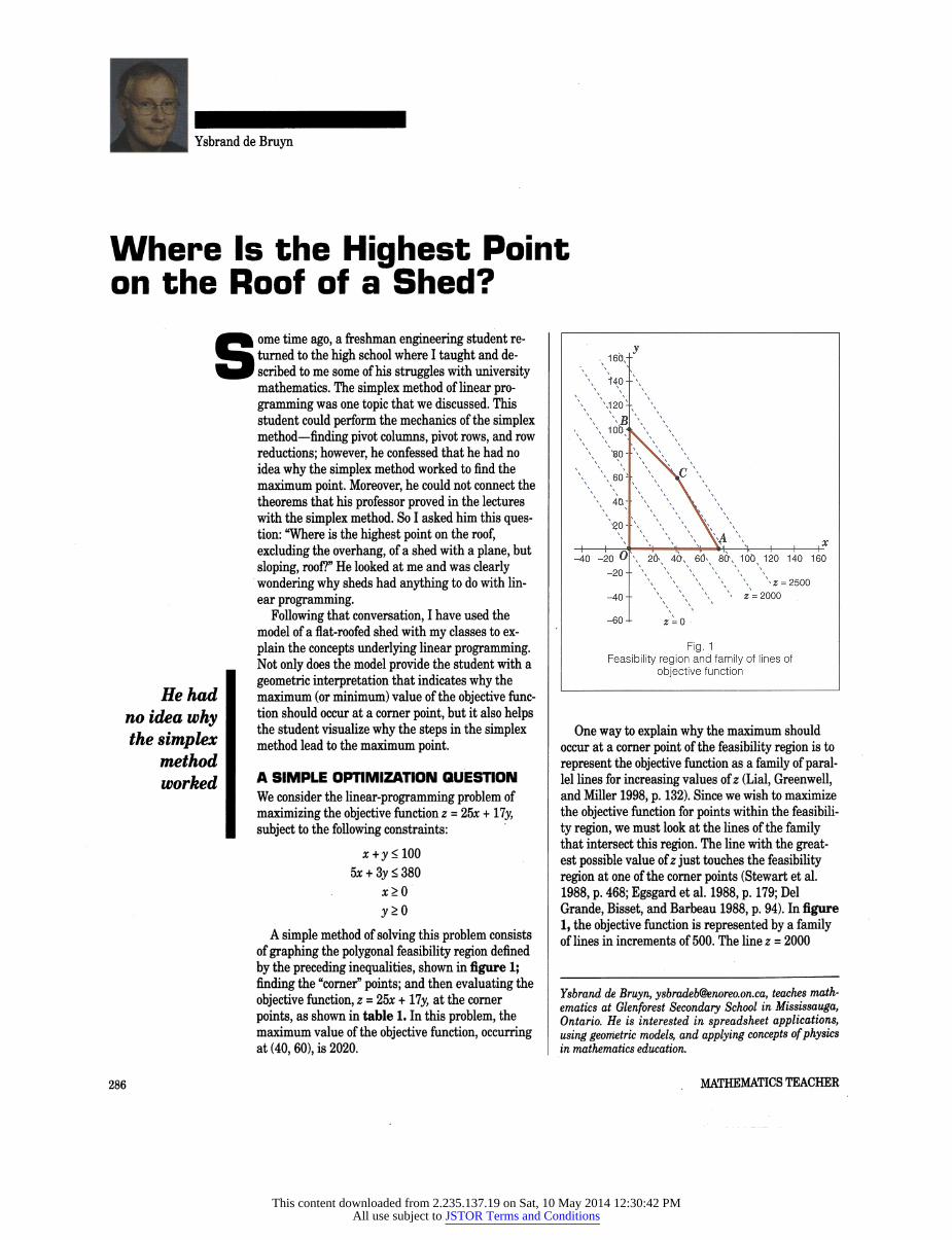
A SIMPLE OPTIMIZATION QUESTION We consider the linear-programming problem of

maximizing the objective function = 25x + 17y, subject to the following constraints:

jc+y<100 5* + 3y < 380

x>0

y>0

A simple method of solving this problem consists of graphing the polygonal feasibility region defined by the preceding inequalities, shown in figure 1; finding the "corner" points; and then evaluating the

objective function, = 25x + 17y, at the corner

points, as shown in table 1. In this problem, the maximum value of the objective function, occurring at (40,60), is 2020.

-40 +

-60-L

H -h 2fc 40, 60* 80\ 10? 120 140 160

\ *z = 2500

z = 2000

2 = 0

Fig. 1 Feasibility region and family of lines of

objective function

One way to explain why the maximum should occur at a corner point of the feasibility region is to

represent the objective function as a family of paral lel lines for increasing values of (Liai, Greenwell, and Miller 1998, p. 132). Since we wish to maximize the objective function for points within the feasibili

ty region, we must look at the lines of the family that intersect this region. The line with the great est possible value of just touches the feasibility region at one of the corner points (Stewart et al.

1988, p. 468; Egsgard et al. 1988, p. 179; Del Grande, Bisset, and Barbeau 1988, p. 94). In figure 1, the objective function is represented by a family of lines in increments of 500. The line = 2000

Ysbrand de Bruyn, ysbradeb@enoreo.on.ca, teaches math

ematics at Glenforest Secondary School in Mississauga, Ontario. He is interested in spreadsheet applications, using geometric models, and applying concepts of physics in mathematics education.

286 MATHEMATICS TEACHER

This content downloaded from 2.235.137.19 on Sat, 10 May 2014 12:30:42 PMAll use subject to JSTOR Terms and Conditions

crosses the region just inside point C, so the line = 2020 intersects the region only at C.

A SHED AS PHYSICAL MODEL Another way of looking at this problem is to build a three-dimensional physical model of the linear

programming problem. Once assembled, the model

looks like a "shed" with a plane, but sloping, roof. The objective function is the equation of a plane. It

is represented by the flat "roof of the shed, where the value of the objective function is the height of the roof above the x-y plane. The "floor plan" of the shed is the feasibility region, with the boundary line segments of the feasibility region forming the "walls" of the shed.

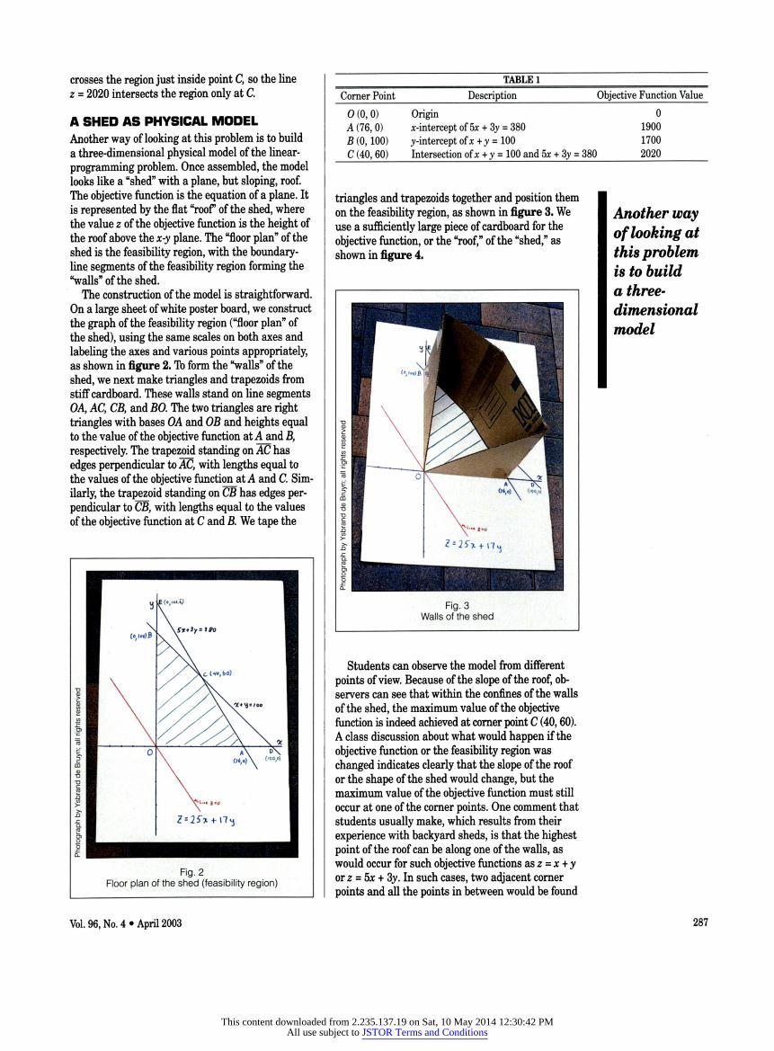
The construction of the model is straightforward. On a large sheet of white poster board, we construct the graph of the feasibility region ("floor plan" of the shed), using the same scales on both axes and

labeling the axes and various points appropriately, as shown in figure 2. lb form the "walls" of the

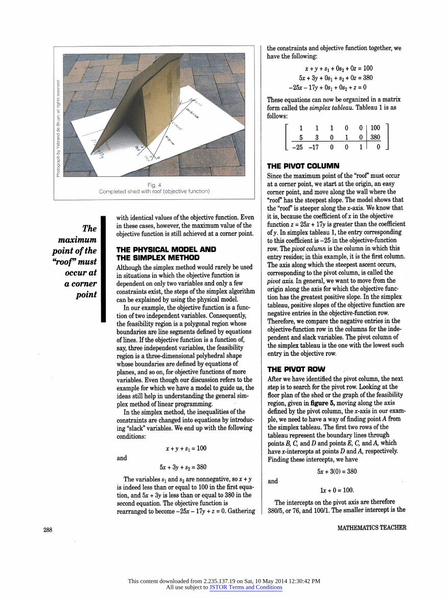
shed, we next make triangles and trapezoide from stiff cardboard. These walls stand on line segments OA, AC, CB, and BO. The two triangles are right triangles with bases OA and OB and heights equal to the value of the objective function at A and B,

respectively. The trapezoid standing on AC has

edges perpendicular to AC, with lengths equal to the values of the objective function at A and C. Sim

ilarly, the trapezoid standing on CB has edges per

pendicular to CB, with lengths equal to the values of the objective function at C and B. We tape the

Fig. 2 Floor plan of the shed (feasibility region)

_TABLE 1_ Corner Point_Description_Objective Function Value

0(0,0) Origin 0 A (76,0) *-interceptof5x + 3y = 380 1900

(0,100) y-intercept of +y = 100 1700 C (40,60) Intersection of + y = 100 and 5* + 3y = 380_2020_

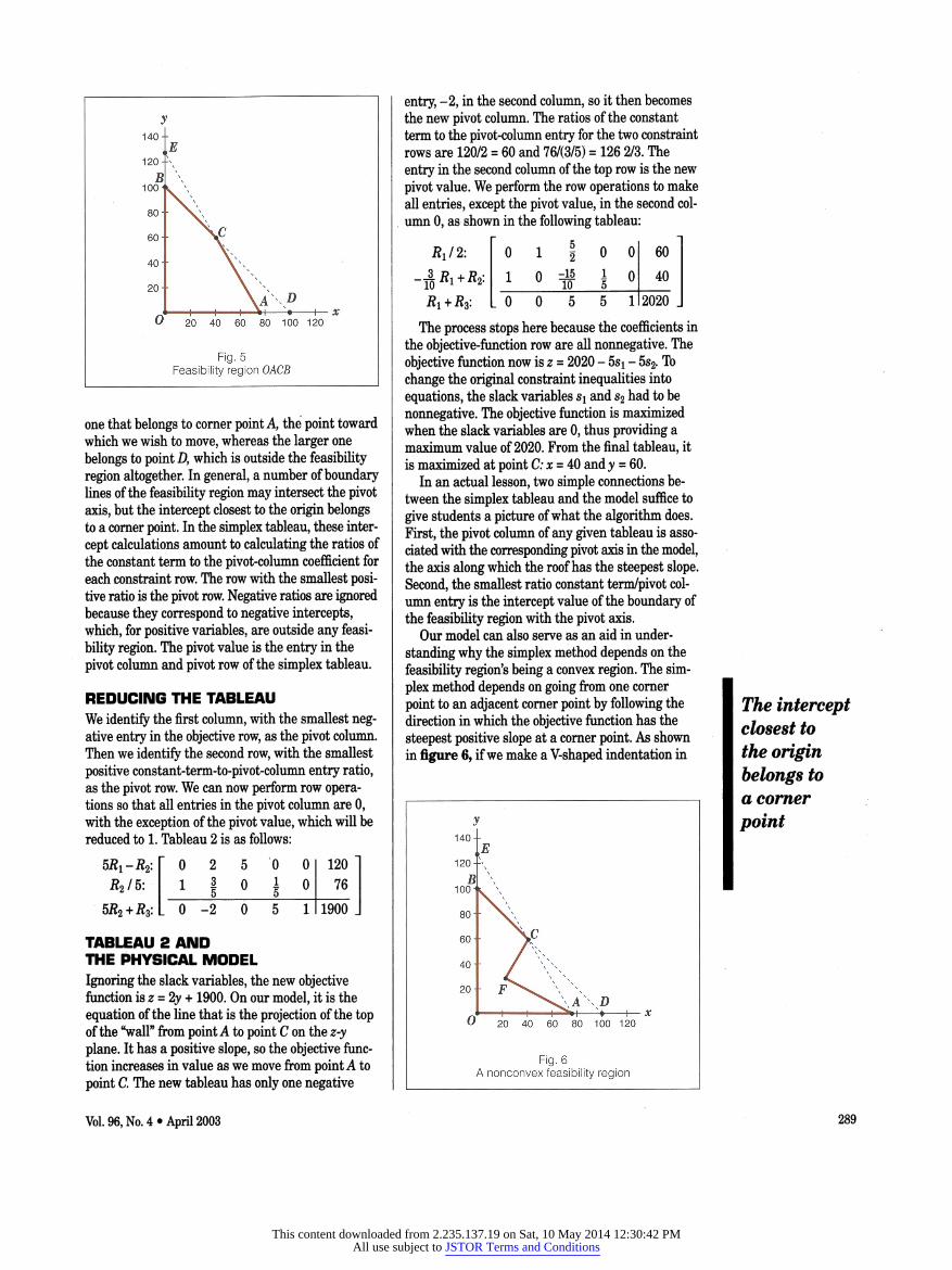
triangles and trapezoids together and position them on the feasibility region, as shown in figure 3. We use a sufficiently large piece of cardboard for the

objective function, or the "roof," of the "shed," as

shown in figure 4.

Another way of looking at this problem is to build a three

dimensional

model

Students can observe the model from different

points of view. Because of the slope of the roof, ob servers can see that within the confines of the walls

of the shed, the maximum value of the objective function is indeed achieved at corner point C (40,60).

A class discussion about what would happen if the

objective function or the feasibility region was

changed indicates clearly that the slope of the roof or the shape of the shed would change, but the maximum value of the objective function must still occur at one of the corner points. One comment that students usually make, which results from their

experience with backyard sheds, is that the highest point of the roof can be along one of the walls, as would occur for such objective functions as = + y or = 5x + 3y. In such cases, two adjacent corner

points and all the points in between would be found

Vol. 96, No. 4? April 2003 287

This content downloaded from 2.235.137.19 on Sat, 10 May 2014 12:30:42 PMAll use subject to JSTOR Terms and Conditions

The maximum

point of the

"roof must occur at a corner

point

with identical values of the objective function. Even in these cases, however, the maximum value of the

objective function is still achieved at a corner point.

THE PHYSICAL MODEL AND THE SIMPLEX METHOD Although the simplex method would rarely be used in situations in which the objective function is

dependent on only two variables and only a few

constraints exist, the steps of the simplex algorithm can be explained by using the physical model.

In our example, the objective function is a func tion of two independent variables. Consequently, the feasibility region is a polygonal region whose boundaries are line segments defined by equations of lines. If the objective function is a function of, say, three independent variables, the feasibility region is a three-dimensional polyhedral shape whose boundaries are defined by equations of

planes, and so on, for objective functions of more

variables. Even though our discussion refers to the

example for which we have a model to guide us, the

ideas still help in understanding the general sim

plex method of linear programming. In the simplex method, the inequalities of the

constraints are changed into equations by introduc

ing "slack" variables. We end up with the following conditions:

and ?C+y + s1 = 100

5x + 3y + s2 = 380

The variables Si and s2 are nonnegative, so + y is indeed less than or equal to 100 in the first equa tion, and 5x + 3y is less than or equal to 380 in the second equation. The objective function is

rearranged to become -25x - 17y + = 0. Gathering

the constraints and objective function together, we have the following:

x+y + S! + 0s2 + 0? = 100

5x + 3y + Osi + s2 + Oz = 380

-25*-17y + 0si + 0s2 + 2 = 0

These equations can now be organized in a matrix

form called the simplex tableau. Tableau 1 is as

follows:

1

0

100 380

-25 -17 0 0 1 I 0 J

THE PIVOT COLUMN Since the maximum point of the "roof must occur

at a corner point, we start at the origin, an easy corner point, and move along the wall where the "roof has the steepest slope. The model shows that

the "roof is steeper along the jc-axis. We know that

it is, because the coefficient of in the objective function = 25x + 17y is greater than the coefficient

of y. In simplex tableau 1, the entry corresponding to this coefficient is -25 in the objective-function row. The pivot column is the column in which this

entry resides; in this example, it is the first column.

The axis along which the steepest ascent occurs,

corresponding to the pivot column, is called the

pivot axis. In general, we want to move from the

origin along the axis for which the objective func

tion has the greatest positive slope. In the simplex tableau, positive slopes of the objective function are

negative entries in the objective-function row.

Therefore, we compare the negative entries in the

objective-function row in the columns for the inde

pendent and slack variables. The pivot column of

the simplex tableau is the one with the lowest such

entry in the objective row.

THE PIVOT ROW After we have identified the pivot column, the next

step is to search for the pivot row. Looking at the floor plan of the shed or the graph of the feasibility region, given in figure 5, moving along the axis defined by the pivot column, the jc-axis in our exam

ple, we need to have a way of finding point A from

the simplex tableau. The first two rows of the

tableau represent the boundary lines through

points B, C, and D and points E, C, and A, which

have ^-intercepts at points D and A, respectively. Finding these intercepts, we have

and

5x + 3(0) = 380

ls + 0 = 100.

The intercepts on the pivot axis are therefore

380/5, or 76, and 100/1. The smaller intercept is the

MATHEMATICS TEACHER

This content downloaded from 2.235.137.19 on Sat, 10 May 2014 12:30:42 PMAll use subject to JSTOR Terms and Conditions

A D -4-1?

20 40 60 80 100 120

Fig. 5

Feasibility region OACB

one that belongs to corner point A, the point toward which we wish to move, whereas the larger one

belongs to point D, which is outside the feasibility region altogether. In general, a number of boundary lines of the feasibility region may intersect the pivot axis, but the intercept closest to the origin belongs to a corner point. In the simplex tableau, these inter

cept calculations amount to calculating the ratios of

the constant term to the pivot-column coefficient for each constraint row. The row with the smallest posi tive ratio is the pivot row. Negative ratios are ignored because they correspond to negative intercepts, which, for positive variables, are outside any feasi

bility region. The pivot value is the entry in the pivot column and pivot row of the simplex tableau.

REDUCING THE TABLEAU We identify the first column, with the smallest neg ative entry in the objective row, as the pivot column. Then we identify the second row, with the smallest

positive constant-term-to-pivot-column entry ratio, as the pivot row. We can now perform row opera tions so that all entries in the pivot column are 0, with the exception of the pivot value, which will be reduced to 1. Tableau 2 is as follows:

5i?i ? R2.

R2/5:

5R2 + ?3:

0 2 5 0 0 1 I 0 ? 0 0 -2

120 76

1900 J

TABLEAU 2 AND THE PHYSICAL MODEL Ignoring the slack variables, the new objective function is = 2y + 1900. On our model, it is the

equation of the line that is the projection of the top of the "wall" from point A to point C on the z-y

plane. It has a positive slope, so the objective func tion increases in value as we move from point A to

point C. The new tableau has only one negative

entry, -2, in the second column, so it then becomes the new pivot column. The ratios of the constant term to the pivot-column entry for the two constraint rows are 120/2 = 60 and 76/(3/5) = 126 2/3. The entry in the second column of the top row is the new

pivot value. We perform the row operations to make all entries, except the pivot value, in the second col umn 0, as shown in the following tableau:

RJ2: 1

0 $ 0 1 5

0 0 1

60

40

2020 J

The process stops here because the coefficients in

the objective-function row are all nonnegative. The

objective function now is = 2020 - 5si -

5s2. To

change the original constraint inequalities into

equations, the slack variables s_ and s2 had to be

nonnegative. The objective function is maximized when the slack variables are 0, thus providing a

maximum value of 2020. From the final tableau, it is maximized at point C: = 40 and y = 60.

In an actual lesson, two simple connections be tween the simplex tableau and the model suffice to

give students a picture of what the algorithm does.

First, the pivot column of any given tableau is asso

ciated with the corresponding pivot axis in the model, the axis along which the roof has the steepest slope. Second, the smallest ratio constant term/pivot col umn entry is the intercept value of the boundary of the feasibility region with the pivot axis.

Our model can also serve as an aid in under

standing why the simplex method depends on the feasibility region's being a convex region. The sim

plex method depends on going from one corner

point to an adjacent corner point by following the direction in which the objective function has the

steepest positive slope at a corner point. As shown in figure 6, if we make a V-shaped indentation in

y 140

120 E

i\A\D 20 40 60 80 100 120

Fig. 6 A nonconvex feasibility region

The intercept closest to

the origin belongs to a corner

point

Vol. 96, No. 4? April 2003 289

This content downloaded from 2.235.137.19 on Sat, 10 May 2014 12:30:42 PMAll use subject to JSTOR Terms and Conditions

the feasibility region of the linear-programming example that we discussed between points A and C in figure 1, we easily see that the maximum value of the objective function still occurs at point C; how

ever, the simplex method fails because the roof of our "shed" and objective function follow a down ward slope from point A to point Ff before going back up to point C.

Second, the objective function in our example depends on only two independent variables, so that the feasibility region is a simple polygon in the plane. Some students will undoubtedly point out

THE ALL NEW

MATHEMATICA TEACHER'S EDITION

RESEARCH

www.wolfram.com/teachersedition To purchase Mathematica Teacher's EiStion, cd) toR free 1WW01FRAM, send emerito infc@wcta.com, or go to store.wolfram.com. ? 2003 Wolfram Research, Ine Mathematica is o registered trademark of Wolfram Research, Inc. Mathematica is not associated with Mtrrhernatka Policy Research, Inc. or MathTech, Inc.

that we can get to the maximum point C by going from O to S and then to C and that the column in the tableau that is reduced first really should not matter. In the general linear-programming prob lems, the objective function depends on three or

more variables. The feasibility region for such a

problem is a "volume" in three or more dimensions. The corner points of the feasibility region may be connected with many other corner points, not just two, so we need to have a definite way to decide the corner point to move to next. The simplex method, in fact, not only chooses the direction of steepest ascent to an adjacent corner point but also rejects the phantom points that are intercepts of boundary "planes" with one of the variable axes but that are not actually corner points of the feasibility region.

One of the grade 9-12 expectations in Principles and Standards for School Mathematics (NCTM 2000, p. 308) is "use of geometric models to gain insight into... other areas of mathematics." The use of the model has certainly helped my students understand the concepts underlying linear pro gramming. In teaching situations in which a com

plete proof is not possible, the model provides stu dents with some measure of confidence in the

validity of the simplex algorithm as a way of mov

ing from one corner point to an adjacent one in such a way that they progress to the point where the maximum occurs. We can only speculate whether

George Dantzig, the original developer of the sim

plex method (O'Connor and Robertson 1996), used

geometrical intuition to guide his investigations.

BIBLIOGRAPHY Del Grande, John J., W. Bisset, and Edward Barbeau. Finite Mathematics. Markham, Ontario: Houghton Mifflin Canada, 1988.

Egsgard, John, Gary Flewelling, Craig Newell, and

Wendy Warburton. Finite Mathematics: A Search for Meaning. Toronto: Gage Educational Publishing Co., 1988.

Liai, Margaret L., Raymond N. Greenwell, and Charles D. Miller. Finite Mathematics. 6th ed. Don Mills, Ontario: Addison-Wesley Educational Publish ers, 1998.

National Council of Teachers of Mathematics (NCTM). Principles and Standards for School Mathematics. Reston,Va.: NCTM, 2000.

Noble, Ben, and James W. Daniel. Applied Linear Algebra. 2nd ed. Englewood Cliffs, N.J.: Prentice Hall, 1977.

O'Connor, J. J., and E. F. Robertson. "George Dantzig." www-gap.dcs.st-and.ac.uk/~history/Mathematicians

/Dantzig_George.html. World Wide Web, 1996. Stewart, James., Thomas M. K. Davidson, 0. Michael G. Hamilton, James Laxton, and M. Patricia Lenz. Finite Mathematics. Toronto: McGraw-Hill Ryerson Limited, 1988.

Mr

290 MATHEMATICS TEACHER

This content downloaded from 2.235.137.19 on Sat, 10 May 2014 12:30:42 PMAll use subject to JSTOR Terms and Conditions