Which Fundamentals Drive Exchange Rates? A Cross … · Which Fundamentals Drive Exchange ... Which Fundamentals Drive Exchange Rates? A Cross-Sectional Perspective ... and investigates

Which Fundamentals Drive Exchange Rates?A Cross-Sectional Perspective∗

Lucio Sarno‡ Maik Schmeling∗∗

This version: April 4, 2013

∗We are grateful to Ken West (editor), two anonymous referees, Lukas Menkhoff and Michael Moorefor very valuable comments and suggestions. Sarno acknowledges financial support from the Economic andSocial Research Council (No. RES-062-23-2340). Schmeling gratefully acknowledges financial support by theGerman Research Foundation (DFG).‡Cass Business School, London and Centre for Economic Policy Research (CEPR). Corresponding author:

Faculty of Finance, Cass Business School, City University London, 106 Bunhill Row, London EC1Y 8TZ,UK, Tel: +44 20 7040 8772, Fax: +44 20 7040 8881, Email: [email protected].∗∗Faculty of Finance, Cass Business School, City University London, 106 Bunhill Row, London EC1Y 8TZ,

UK, Email: [email protected].

Which Fundamentals Drive Exchange Rates?A Cross-Sectional Perspective

Abstract

Standard present-value models suggest that exchange rates are driven by expected

future fundamentals, implying that current exchange rates contain predictive informa-

tion about future fundamentals. We test the validity of this key empirical prediction

of present-value models in a sample of 35 currency pairs ranging from 1900 to 2009.

Employing a variety of tests, we find that exchange rates have strong and significant

predictive power for nominal fundamentals (inflation, money balances, nominal GDP),

whereas predictability of real fundamentals and risk premia is much weaker and largely

confined to the post-Bretton Woods era. Overall, we uncover ample evidence that

future macro fundamentals drive current exchange rates.

JEL Classification: F31; G10.

Keywords: Exchange rates; economic fundamentals; forecasting; present value model.

1. INTRODUCTION

Whether exchange rates are linked to observable macroeconomic fundamentals has long been

controversial in the literature and there is early evidence against such a link dating back to

the work of Meese and Rogoff (1983), leading to the so-called “disconnect puzzle”.

However, the well-documented finding that exchange rates are only weakly related to con-

temporaneous (or lagged) macro fundamentals does not mean that exchange rates are truly

“disconnected” from fundamentals. In fact, Engel and West (2005) show that the appar-

ently weak relationship between exchange rates and fundamentals can be reconciled within

a standard present-value model of asset prices when discount factors are close to unity and

fundamentals are nonstationary. In this setting, the exchange rate can be entirely driven by

macro fundamentals but the link is such that expectations about future macro fundamentals

drive current exchange rates, whereas current and lagged fundamentals are relatively unim-

portant. Hence, to identify which fundamentals matter most for exchange rates, it is sensible

to test for predictability of fundamentals by using lagged exchange rates as predictors.1

Engel and West (2005) were the first to provide evidence that exchange rates do indeed

Granger-cause fundamentals, a finding which suggests that there is a sensible connection be-

tween fundamentals and exchange rates after all. Related to this, Engel and West (2006) find

that deviations of real exchange rates from steady state values forecast inflation and output

gaps. In a similar vein, Chen, Rogoff, and Rossi (2010) find that “commodity currencies”

robustly forecast commodity prices.

1Quoting Obstfeld and Rogoff (2000, p. 373) : ‘[...] the exchange-rate disconnect puzzle [...] alludesbroadly to the exceedingly weak relationship (except, perhaps, in the longer run) between the exchange rateand virtually any macroeconomic aggregates. It manifests itself in a variety of ways. For example, Meeseand Rogoff (1983) showed that standard macroeconomic exchange-rate models, even with the aid of ex-postdata on the fundamentals, forecast exchange rates at short to medium horizons no better than a naive randomwalk.’ Indeed, there is evidence in favor of a sensible predictive relationship from macro factors to exchangerates only at rather long horizons (e.g. Mark, 1995; Mark and Sul, 2001; Abhyankar, Sarno, and Valente,2005). However, to be clear, this is not the aspect of the puzzle on which we focus in this paper. Insteadwe focus on the other side of the puzzle that refers to ‘the remarkably weak [...] feedback links between theexchange rate and the rest of the economy’ (Obstfeld and Rogoff, 2000, p. 373) and analyze whether andhow fluctuations in the exchange rate are related to future aggregate macroeconomic variables.

1

Hence, there is some evidence that exchange rates forecast fundamentals, which implies that

(expected) fundamentals do indeed matter for exchange rates. However, the evidence is

confined to a relatively small set of currencies and economic variables, to the recent floating

exchange rate regime since the 1970s, and to tests applied to individual currency pairs.

Yet the empirical prediction of the Engel-West framework is very general, and several key

fundamental variables qualify as being relevant for exchange rates even in standard exchange

rate models. This paper provides a fresh and comprehensive assessment of this prediction

of present-value models, and investigates whether exchange rate movements have predictive

power for a number of relevant macro fundamentals in a large cross-section of countries over

a century-long sample. The cross-sectional aspect of our data is especially important since

it allows us to conduct tests which average out most of the idiosyncratic noise in individual

exchange rates and, thus, to carry out more powerful tests. The key questions that guide

our analysis are: (i) is there a link between current exchange rates and future fundamentals

consistent with standard present-value models of the exchange rate, and, if so, (ii) which

fundamentals matter most? Answers to these questions seem relevant as they have direct

implications - among other things - for theoretical exchange rate modeling.

Our empirical analysis is based on long-run data for 35 currencies quoted against the US

Dollar (USD) covering the period from 1900 to 2009. In many of our tests, we take a

perspective typical of the finance literature, relying mainly on a simple and model-free out-of-

sample forecasting exercise and forming groups (or portfolios) of countries depending on their

lagged spot rate movements against the USD. The composition of these groups is updated

each year and we examine the macro performance of these different groups of countries

throughout each annual forecasting period. In addition, we also present results based on

more conventional panel regressions (controlling for fixed country and time effects).

Our results show that countries whose currencies strongly appreciated against the USD in

the past have significantly lower future inflation, growth in money balances, nominal GDP

growth, and interest rates, compared to countries whose currencies most strongly depreci-

ated against the USD. The differences in fundamentals’ growth rates across the two groups of

countries is statistically and economically significant and easily exceeds 10% p.a. for inflation

2

and money growth. These relations are very robust across sample periods and test methods,

suggesting that future nominal fundamentals matter a lot for current exchange rates. Fur-

ther nominal variables, such as interest rate differentials and risk premia (deviations from

uncovered interest rate parity) also matter, but their importance is largely confined to the

post-Bretton Woods sample.2

We also investigate the existence of predictability for real macroeconomic fundamentals such

as real GDP growth, real money growth, and real exchange rate changes. However, the evi-

dence is not as clear-cut as for nominal fundamentals. We find some evidence of predictability

of real exchange rate changes, especially for the post Bretton Woods sample period, whereas

real GDP growth is not robustly predictable and its relationship with the current spot rate

tends to switch sign across different sample periods. We illustrate, however, how the latter

finding can be rationalized by instabilities in the income elasticity of money demand. Real

money growth seems the least predictable (by means of past exchange rates), and we only

find some predictability at longer horizons.

Finally, it is worthwhile mentioning that almost all predictive relations uncovered in our

empirical work are in line with the theoretical predictions (which we turn to in the next

section) from a standard monetary exchange rate model. Hence, our findings in a nutshell are

as follows. First, fundamentals matter a lot for exchange rates empirically, and it seems that

nominal fundamentals are more important than real fundamentals. Second, fundamentals

matter in a way consistent with standard present-value logic as exchange rate movements

forecast fundamentals. Third, fundamentals generally tend to matter in a way consistent with

standard monetary exchange rate models, a workhorse of traditional international finance.

Fourth, our main results are robust across methods and also hold when controlling for lagged

macro fundamentals.3

2Froot and Ramadorai (2005) find that (expectations about) risk premia are a strong driver of realexchange rates in a VAR-based decomposition based on recent data. Hence, their result is by and largecompatible with ours although we are investigating nominal exchange rates.

3However, as noted later in the paper, our results are also consistent with other theoretical arguments dif-ferent from the standard present-value model we choose to focus on. Specifically, it is clear that fundamentalsare endogenous and determined jointly with exchange rates in equilibrium, so that the predictability fromexchange rates to fundamentals documented here should not be taken necessarily as unidirectional causality.

3

The paper proceeds as follows. The next section briefly reviews theoretical concepts. Section

3 details the data. Section 4 describes the empirical approach and results. Section 5 provides

additional results and robustness, and Section 6 concludes. A separate Internet Appendix to

this paper contains additional information and robustness results.

2. THEORETICAL MOTIVATION

The asset price approach to exchange rates relies on the fact that the exchange rate, as any

other asset price, can be written as the discounted present value of future fundamentals:

st = (1− b)∞∑i=0

biEt[ft+i] (1)

where s is the log nominal exchange rate, b is a parameter that depends on the structure of an

underlying macro model, and f denotes the set of macro fundamentals. The above present-

value formulation starts from the general idea that spot rates are driven by fundamentals

and expected spot rates, i.e.

st = (1− b)ft + bEt[st+1] (2)

and Eq. (1) then follows from iterating forward Eq. (2) provided that the no-bubbles

condition biEt[st+i] = 0 holds for i→∞ and that current fundamentals are observable. Thus,

Eq. (1) suggests that current exchange rates should be informative for future fundamentals.

The general formulation in Eq. (1) takes no stand on which fundamentals to include in

exchange rate determination so that the menu of fundamentals will be driven by choosing

a particular exchange rate model. For our empirical application below, we rely on a fairly

standard but general setup based on the monetary exchange rate model, which is described

in Eq. (7) in Engel and West (2005)

st =1

1 + α[− (m∗t −mt) + γ (y∗t − yt) + (v∗mt − vmt) + qt − αρt] +

α

1 + αEt[st+1] (3)

4

where s is the log spot exchange rate expressed as US dollars per foreign currency unit (USD

per FCU), m is the log of the money supply, y is (real) output, vm is a money demand shock,

q denotes the log real exchange rate defined as qt = st−p∗t +pt, and ρ is the foreign exchange

risk premium (i.e. the deviation from uncovered interest rate parity, ρt = ∆st + i∗t − it); the

(log) price level is denoted as pt, and it is the continuous short-term interest rate. Asterisks

indicate variables of the foreign country. Finally, γ is the income elasticity of the demand

for money and α is the interest rate semi-elasticity of money demand. We refer to Engel and

West (2005) and Engel, Mark, and West (2007) for further details of this specification but

note here that it is fairly general and does not impose uncovered interest parity.

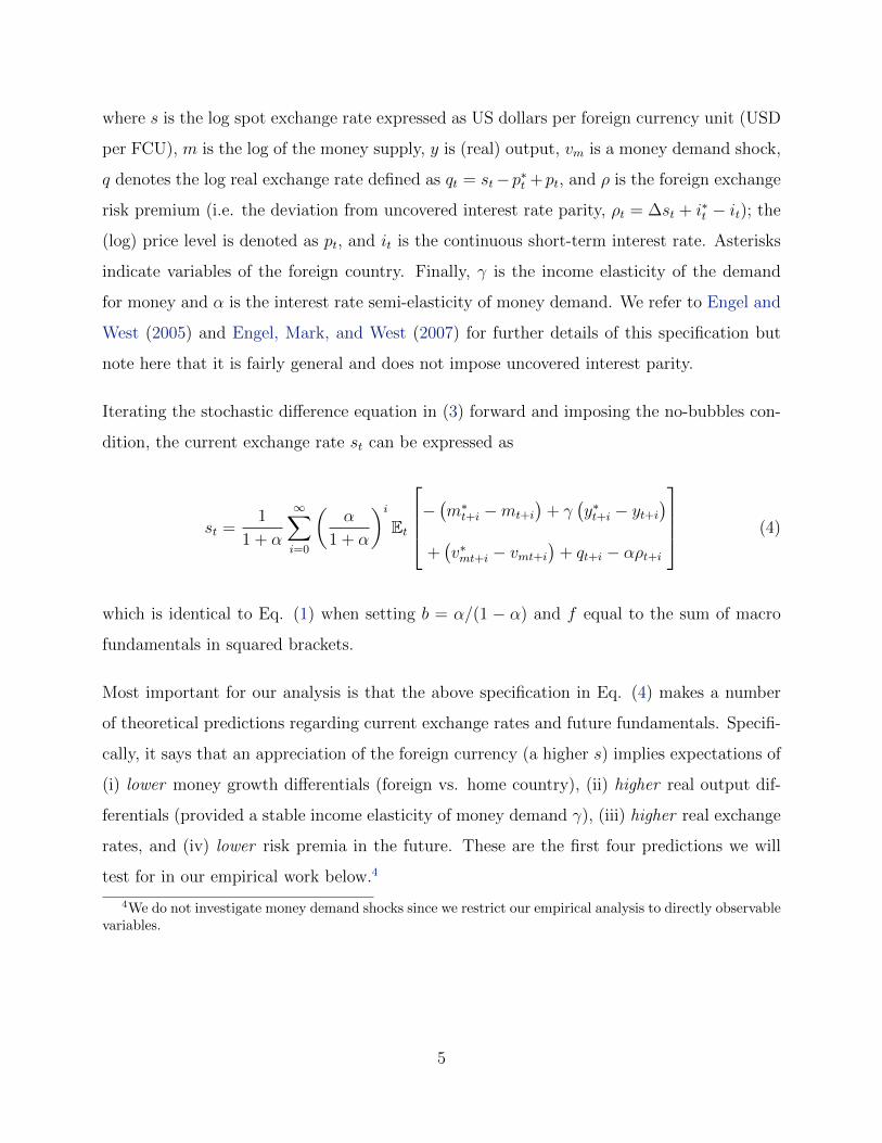
Iterating the stochastic difference equation in (3) forward and imposing the no-bubbles con-

dition, the current exchange rate st can be expressed as

st =1

1 + α

∞∑i=0

(α

1 + α

)iEt

−(m∗t+i −mt+i

)+ γ

(y∗t+i − yt+i

)+(v∗mt+i − vmt+i

)+ qt+i − αρt+i

(4)

which is identical to Eq. (1) when setting b = α/(1 − α) and f equal to the sum of macro

fundamentals in squared brackets.

Most important for our analysis is that the above specification in Eq. (4) makes a number

of theoretical predictions regarding current exchange rates and future fundamentals. Specifi-

cally, it says that an appreciation of the foreign currency (a higher s) implies expectations of

(i) lower money growth differentials (foreign vs. home country), (ii) higher real output dif-

ferentials (provided a stable income elasticity of money demand γ), (iii) higher real exchange

rates, and (iv) lower risk premia in the future. These are the first four predictions we will

test for in our empirical work below.4

4We do not investigate money demand shocks since we restrict our empirical analysis to directly observablevariables.

5

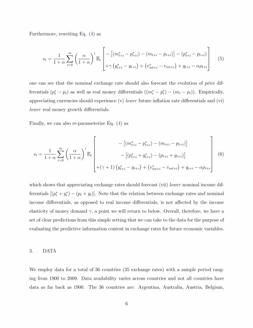
Furthermore, rewriting Eq. (4) as

st =1

1 + α

∞∑i=0

(α

1 + α

)iEt

−[(m∗t+i − p∗t+i)− (mt+i − pt+i)

]− (p∗t+i − pt+i)

+γ(y∗t+i − yt+i


)+ qt+i − αρt+i

(5)

one can see that the nominal exchange rate should also forecast the evolution of price dif-

ferentials (p∗t − pt) as well as real money differentials ((m∗t − p∗t ) − (mt − pt)). Empirically,

appreciating currencies should experience (v) lower future inflation rate differentials and (vi)

lower real money growth differentials.

Finally, we can also re-parameterize Eq. (4) as

st =1

1 + α

∞∑i=0

(α

1 + α

)iEt

−[(m∗t+i − p∗t+i)− (mt+i − pt+i)

]−[(p∗t+i + y∗t+i)− (pt+i + yt+i)

]+(γ + 1)

(y∗t+i − yt+i


)+ qt+i − αρt+i

(6)

which shows that appreciating exchange rates should forecast (vii) lower nominal income dif-

ferentials [(p∗t + y∗t )− (pt + yt)]. Note that the relation between exchange rates and nominal

income differentials, as opposed to real income differentials, is not affected by the income

elasticity of money demand γ, a point we will return to below. Overall, therefore, we have a

set of clear predictions from this simple setting that we can take to the data for the purpose of

evaluating the predictive information content in exchange rates for future economic variables.

3. DATA

We employ data for a total of 36 countries (35 exchange rates) with a sample period rang-

ing from 1900 to 2009. Data availability varies across countries and not all countries have

data as far back as 1900. The 36 countries are: Argentina, Australia, Austria, Belgium,

6

Brazil, Canada, Denmark, Finland, France, Germany, Greece, Hong Kong, India, Indonesia,

Ireland, Israel, Italy, Japan, (South) Korea, Mexico, Netherlands, New Zealand, Norway,

Portugal, Saudi Arabia, Singapore, South Africa, Spain, Sweden, Switzerland, Taiwan, Thai-

land, Turkey, United Kingdom, United States, and Venezuela. While the full-sample analysis

covers the longest time span available to us from 1900 to 2009 for each country, we addition-

ally work with a sub-sample from 1974 to 2009 to cover a recent time period characterized

by relatively open and integrated markets over the post-Bretton Woods period.

For each country, we have available information on spot exchange rates, the consumer price

index (CPI), gross domestic product (GDP), money balances (currency in circulation), and

short-term interest rates (T-Bills). We obtain these data from Global Financial Data (GFD),

which provides access to a host of long-run macro and financial time series. Note that some

countries do not have all data available for the full sample period and therefore enter the

sample later. Also, we eliminate all euro member countries from the sample in the year of

the actual adoption of the euro. Due to data availability, we have to employ annual data for

CPI inflation, money growth, and GDP growth.

Spot exchange rates as well as CPI, GDP and money balances are measured at the end of

each year and are not yearly averages. To ensure stationarity, we employ annual (log) changes

of all macro variables (except for interest rates) in the subsequent analysis. Interest rate data

are available at higher frequencies but we use annual data, measured at the end of each year,

for consistency. We take the U.S. to be the home country and investigate exchange rates,

growth rate differentials and interest rate differentials relative to the U.S. Table 1 shows

median growth rates of our macro fundamentals and their availability across countries.5 We

present medians since our data include several time-country combinations of hyperinflations

which dominate average growth rates and interest rates. For this reason, we later check the

robustness of our results using winsorized time-series of exchange rates, interest rates, and

macro fundamentals such that values above (below) the 95th percentile (5th percentile) are

5Most exchange rate series extend back to 1900 so that macro variables effectively determine data avail-ability across countries.

7

set to the 95th percentile (5th percentile).6

Table 1 about here

4. EMPIRICAL RESULTS

4.1. Forming country portfolios

Methodology. To investigate whether spot rates have predictive power for macro fun-

damentals in the cross-section of countries we mainly rely on a simple and robust method

borrowed from the finance literature for most of our empirical analysis. Specifically, we form

groups (or portfolios) of countries at the end of each year based on their lagged stochastically

detrended spot rate (against the USD). The stochastically detrended spot rate (S) is simply

the log spot rate (s) minus its (log) average over the previous ten years (st−9;t):

St = st − st−9;t (7)

where exchange rates are in USD per FCU as in the theoretical discussion above so that

higher values of S mean that the foreign currency has appreciated against the USD relative

to its recent past.

We allocate the 25% of all countries with the lowest spot rate change (i.e. the largest de-

preciation against the USD) to group one (G1) and the 25% of all countries with the largest

appreciation against the USD to group four (G4), with the remaining countries being allo-

cated to the intermediate groups two or three (G2 and G3, respectively). These groups of

countries, or country portfolios, then remain unchanged for one calendar year and we track

their growth differential against the U.S. with respect to CPI inflation, money balances, nomi-

6Note that we winsorize the growth rates of macro variables and detrended exchange rates and not thelevel of these variables themselves. The results using winsorized data indicate that our findings do not changequalitatively.

8

nal GDP, real money balances, and real GDP. In addition, we also compute risk premia (UIP

deviations) as well as short-term interest rate differentials and real exchange rate changes

against the U.S. over the year following the formation of groups.

Starting at the end of 1909, so that 1910 is our first forecast period, we then repeat this

procedure each year to obtain time series of growth rate (and interest rate) differentials

against the U.S. for each of the macro variables listed above and for each of the four portfolios.

The dynamic rebalancing of country groups hence enables us to look at the future macro

performance of groups of countries with relatively similar past exchange rate depreciations.

A simple test of cross-sectional predictability amounts to testing whether there is a significant

difference between growth rate differentials of G1 versus G4.7 Note that taking the difference

between two country portfolios, e.g. G1 and G4, effectively cancels out the U.S. component

of growth differentials and interest rates so that we are looking at macro growth and interest

rate differentials between the two respective groups of countries.

We employ this procedure for two main reasons. First, because it enjoys a number of advan-

tages over standard regression approaches for the questions we want to examine. Forming

portfolios of countries and investigating their average growth rate differentials is nonpara-

metric in the sense that we do not have to assume a specific functional relationship between

lagged spot rate movements and future macro growth rates. While we would expect, for

example, a monotonically declining pattern of money growth differentials when moving from

G1 to G4 based on prediction (i) of the monetary model, the pattern across country portfo-

lios may empirically be increasing, decreasing, or hump-shaped and employing the portfolio

approach easily allows for all of these possible patterns.8 In addition, the portfolio formation

approach naturally handles unbalanced panels of data where countries enter the sample at

different times (or drop out of the sample, e.g., due to the adoption of the euro). Also,

predictive regressions involving persistent predictive variables are prone to biases and statis-

7As noted above, this procedure is heavily used in the finance literature in the context of equity or bondportfolios. However, this approach has also been used in the international finance literature, e.g. in thecontext of currency portfolios (see Lustig and Verdelhan, 2007; Menkhoff, Sarno, Schmeling, and Schrimpf,2012a,b).

8We do find very similar results with a linear panel regression approach below, however, so that allowingfor non-linearities does not seem to be overly important in establishing our empirical results.

9

tical problems with nominal significance levels (see e.g. Stambaugh, 1999), which we avoid

by directly investigating the spread of growth differentials across country groups.9 Second,

this approach yields results which are readily interpretable in terms of economic significance

in an out-of-sample setting, which is our main object of interest. The difference in growth

differentials between G1 and G4 directly yields an estimate of how much higher the growth

of a given macro factor is in countries with “weak” versus “strong” exchange rates. However,

we also complement our main approach of forming portfolios of countries with more standard

panel regressions below, for robustness.

Finally, we briefly discuss our choice of predictive variable, namely, the detrended spot ex-

change rate against the USD. Theory predicts that the spot rate itself should predict future

changes in macro fundamentals. However, and as noted in Engel and West (2005), using the

level of the spot rate directly can be problematic due to lack of stationarity. Hence, we opt

to look at spot rates detrended over the previous ten years to accomplish two things. First,

the horizon is long enough to net out short-term noise in exchange rate movements (which

we are not interested in) but short enough so that nonstationarity does not become problem-

atic.10 Second, detrended spot rates represent deviations in percent and are, thus, directly

comparable across countries and useful for sorting countries into portfolios. However, we also

compute results based on simple one-year and ten-year (log) exchange rate changes instead

of detrended spot rates for all major analyses, and find that our results are not driven by the

specific choice of the detrended exchange rate.

Main results. Next we report our main results based on country portfolios. For robustness,

we report results based on raw fundamentals and results based on winsorized fundamentals.

To start with, the left part of Table 2, Panel A, shows average growth rate differentials

(against the U.S.) for CPI inflation for all four groups of countries (G1 – G4) and the dif-

9This is relevant in our case when using the detrended exchange rate which is indeed persistent. Forexample, the average first-order autoregressive coefficient for the detrended spot exchange rate across all 35currency pairs is estimated to be 0.83, with a cross-sectional standard deviation of 0.08; the maximum is 0.96and the minimum is 0.61. Hence, statistical inference in predictive regressions in this case would have to takeaccount of this persistence, which is notoriously cumbersome.

10We have also experimented with somewhat shorter horizons (e.g. down to horizons of five years) andfound that the results reported below are not affected qualitatively.

10

ference in average growth rates between G4 and G1 (“Diff”). Panel F shows the same for

winsorized fundamentals. Numbers in brackets are t-statistics based on Newey and West

(1987) standard errors. We report results both for the full sample period from 1910 to 2009

and for a shorter subperiod from 1974 to 2009. The latter sample period mainly serves as

a control for robustness to see whether results for the full period also extend to the post-

Bretton Woods era with relatively open capital markets, market integration, and exchange

rate convertibility.11

We find that future CPI inflation is indeed much higher in countries whose currencies expe-

rienced the strongest depreciation against the USD over the previous ten years (G1) relative

to countries whose currencies most strongly appreciated against the USD (G4). More specif-

ically, the average annual difference in CPI growth against the U.S. for the full sample period

is about 23% (15% for winsorized CPI inflation) for country portfolio G1 and declines mono-

tonically when moving to G2 and G3 to a growth rate differential of about zero for countries

with a strong appreciation against the USD in G4. Hence, there is a massive difference in

growth rates of -23.32% (-14.77% for winsorized data), which is highly significant. Also, we

find a very similar result when restricting the sample to the post-Bretton Woods period. In

sum, it appears that lagged spot rate movements have significant predictive power for future

inflation in the cross-section of countries, and that this predictive power is economically sig-

nificant. More importantly, the pattern in inflation differentials squares well with economic

intuition and the predictions from traditional models of exchange rate determination outlined

in Section 2.

Table 2 about here

Table 2 also reports the same kind of information for growth differentials in money balances

(Panels B and G) and nominal GDP (Panels C and H). The evidence is very similar, and

11We are aware of the fact that the full sample period covers different exchange rate regimes and thatpredictability of fundamentals by exchange rates might be different during fixed and floating exchange rateregimes. However, it seems a natural starting point to look at a very long sample period which containsa maximum of variability in fundamentals and exchange rates both in the time-series and cross-sectionaldomain in order to maximize statistical efficiency and economic significance.

11

similarly impressive, for these two macro factors. There is an almost monotonic decline in

growth rates when moving from G1 to G4 for both money and GDP growth differentials and

for both sample periods. The smallest difference (in absolute value) between growth rates

is about 10% for the full sample and winsorized GDP growth, and therefore all differences

are economically large. Hence, spot exchange rates contain a lot of information for future

(nominal) macro movements in the cross-section of countries, and the sign of the predic-

tive relation with future money growth is in line with predictions (i), (v), and (vii) in the

theoretical motivation (Section 2) above.

Furthermore, we investigate whether lagged spot rate movements are informative about future

risk premia (UIP deviations) and report results in Panels D and I of Table 2. Risk premia

are computed as ρt = ∆st + i∗t − it and, since it is well known that exchange rate changes are

hard to forecast at short horizons, we also report results for pure interest rate differentials

i∗t − it in Panels E and J of the same table. As might be expected, we find that there

is no significant predictability for risk premia in the full country sample, which is strongly

dominated by fixed exchange rate regimes. We do find the expected negative pattern (see

prediction (iv) in Section 2 above) for the post Bretton Woods sample, however, although

the difference between G4 and G1 is not statistically significant. As noted above, we also

examine interest rate differentials separately, and we do indeed find clear-cut results in this

case. Specifically, looking at Panel E, there is a monotonically declining pattern in interest

rate differentials when moving from country groups G1 to G4, and the difference between G1

and G4 is highly significant both in economic terms, -3.04% for the full sample and -6.30%

for the later subsample, and in statistical terms with Newey-West based t-values of −3.08

and −3.40. The results are qualitatively identical for winsorized data (Panel J). We take this

as being supportive of prediction (iv).

Next, we investigate the spot rate’s ability to forecast real fundamentals and look at real

money growth, real GDP growth, and real exchange rate changes. We use CPIs to deflate

money balances and GDP, and to compute real exchange rates. Results for this exercise are

reported in Table 3 and show that the evidence for these real variables is somewhat mixed.

Starting with real money growth in Panel A we see some significant evidence in line with the

12

theoretical prediction (vi) for the full sample (about -10% difference between G4 and G1)

but not for the recent float. For winsorized data (Panel D), the results are even weaker in

that we record no predictability for any of the two sample periods.

Results for real output growth (Panels B and E) are mixed. For the full sample, we find no

evidence for the theoretically expected positive relation between exchange rate movements

and output differentials (prediction (ii) in Section 2). Even worse, we find a negative pattern

for the post-Bretton Woods sample, which is small in absolute magnitude but significant in

statistical terms. This finding is striking since it is at odds with one of the central predictions

of the monetary model. However, care must be taken when interpreting the evidence on real

output differentials. Eq. (3) above tells us that exchange rates should forecast real output

differentials multiplied by the income elasticity of money demand. It is well known that the

latter quantity is highly unstable over time in money demand equations, so that it is not

especially surprising to find shaky patterns for this particular variable.12

Next, we find that detrended nominal exchange rates have some predictive power for real

exchange rates (Panels C and F), at least over the recent post Bretton Woods sample. The

pattern is such that countries with appreciating currencies (G4) experience an average in-

crease of 3.08% (2.49% for winsorized data) in their future real exchange rates relative to

countries with depreciating exchange rates (G1). This positive pattern is well in line with the-

ory (prediction (iii) in Section 2) and strongly statistically significant for the non-winsorized

data.

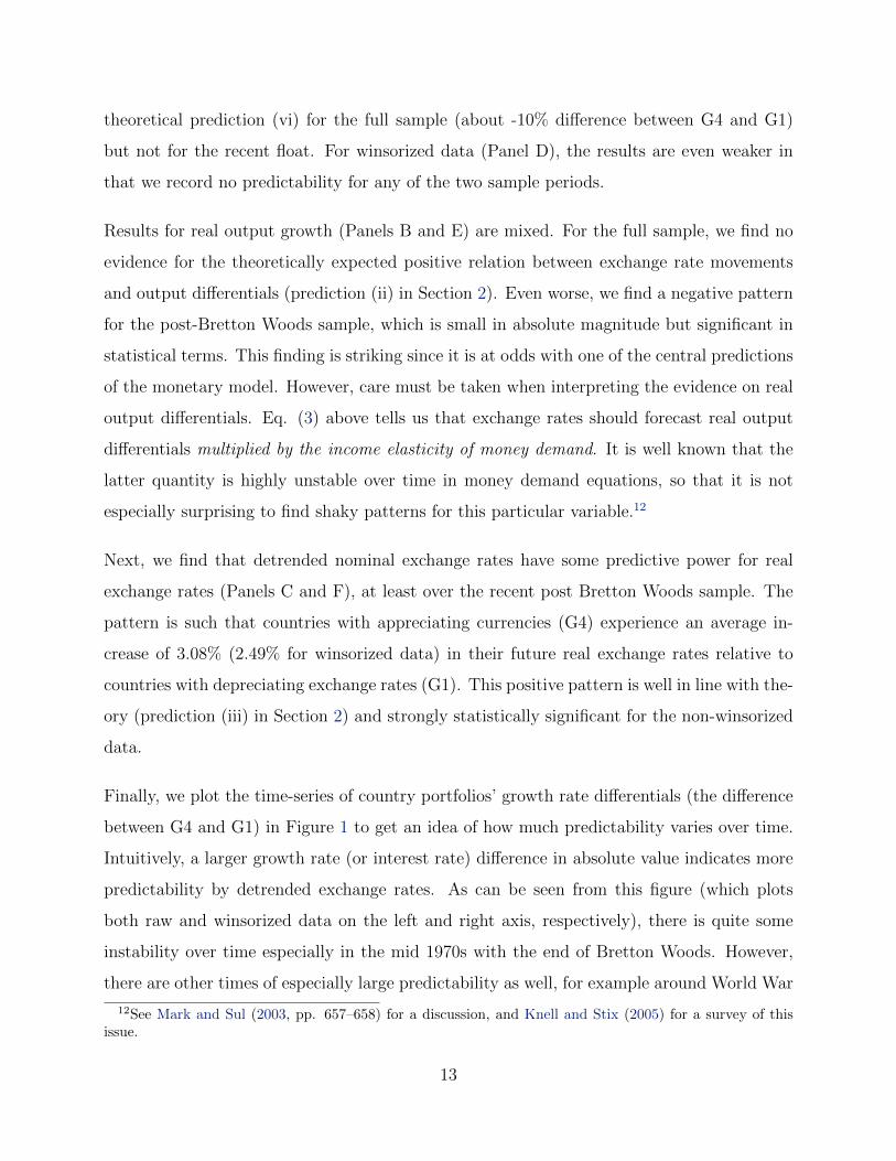
Finally, we plot the time-series of country portfolios’ growth rate differentials (the difference

between G4 and G1) in Figure 1 to get an idea of how much predictability varies over time.

Intuitively, a larger growth rate (or interest rate) difference in absolute value indicates more

predictability by detrended exchange rates. As can be seen from this figure (which plots

both raw and winsorized data on the left and right axis, respectively), there is quite some

instability over time especially in the mid 1970s with the end of Bretton Woods. However,

there are other times of especially large predictability as well, for example around World War

12See Mark and Sul (2003, pp. 657–658) for a discussion, and Knell and Stix (2005) for a survey of thisissue.

13

I and II.

Figure 1 about here

Overall, a fair conclusion seems to be that exchange rates offer less predictive power for

real fundamentals than for nominal fundamentals, although this dichotomy in results is not

directly predicted by theory. In addition, these findings are robust when using ten-year

(log) exchange rate changes st− st−9 instead of detrended exchange rates St as predictors as

shown in Tables A.4 and A.5 in the Internet Appendix. We find no substantial differences.

Similarly, Table A.6 in the Internet Appendix presents results using one-year (log) exchange

rate changes st − st−1 but does not yield new insights and confirms the finding that results

for real macro fundamentals are somewhat shaky and depend on the particular exchange rate

predictor at hand.

Table 3 about here

4.2. Monotonicity tests

To obtain more powerful tests of whether average growth rates are indeed decreasing or

increasing across country portfolios, we employ several recent tests proposed by Patton and

Timmermann (2010), which are designed to handle questions of exactly this kind. We adapt

their general case to our setting with four country portfolios and briefly describe their tests

in the following section.

Methodology. Let ∆i = µi − µi−1 be the difference between average growth rates in a

macro variable i for two adjacent country portfolios. The hypothesis of a decreasing pattern

in average growth rates can be tested by formulating the null and alternative hypotheses as

H0 : ∆i ≥ 0 for i = 2, 3, 4

vs. H1 : ∆i < 0 (8)

14

so that the alternative hypothesis is expected to hold if appreciating exchange rates fore-

cast lower fundamentals’ growth rates (or risk premia and interest rate differentials). More

compactly, with ∆ = [∆2,∆3,∆4], the above null and alternative can also be written as

H0 : ∆ ≥ 0 vs. H1 : ∆ < 0 where vector (in)equalities apply element-wise. Furthermore,

the alternative hypothesis demands that maxi=2,3,4 ∆i < 0, which suggests the test statistic

JT = maxi=2,3,4 ∆̂i, where ∆̂ denotes the sample estimate of differences in average growth

rates µ̂i − µ̂i−1. Patton and Timmermann (2010) suggest a stationary block bootstrap to

compute p-values for this test statistic (Politis and Romano, 1994), which we also employ in

our analysis. We report results based on this test for monotonicity as “MR” in our tables for

all fundamentals except for real output growth and real exchange rate changes. Here, theory

indicates a monotonically increasing pattern so that we reformulate the null and alternative

hypotheses accordingly.

In addition, we report three other test results which are related to the test described above

and which are also described in Patton and Timmermann (2010). First, we report the“MRall”

test which is based not only on differences in average growth of adjacent country groups but

on all pairwise comparisons of country portfolios. Second and third, we report results for“Up”

and “Down” tests, which are somewhat less restrictive than the monotonicity tests (which

require a monotonically declining pattern) and only test for increasing (“Up”) or decreasing

(“Down”) patterns in average growth rates in some parts of the cross-sections. Hence, these

tests are likely to have higher power.

Empirical results. Results for the MR, MRall, “Up”, and “Down” tests can be found in

Tables 2 and 3 in the right part of each table.13 Results from these tests are largely confirma-

tive of our qualitative discussion above. The MR (MRall, Down) tests tend to be significant

for CPI inflation, money growth, and nominal GDP growth differentials (Panels A – C and

F – H of Table 2), especially when looking at the winsorized fundamentals, the only excep-

tion being the MR-tests for non-winsorized money growth differentials (Panel B). Results

13Results for 10-year and 1-year exchange rate changes instead of detrended exchange rates can be foundin Tables A.4, A.5, and A.6 in the Appendix.

15

for risk premia (UIP deviations) and short-term interest rate differentials, respectively, are

reported in Panels D-E and I-J of Table 2. As above, the evidence for risk premia is fairly

weak. However, and similar to our findings above, there is clear evidence for a monotonic

pattern in interest rate differentials. Results for real fundamentals are reported in Table 3.

There is some evidence of a systematically declining pattern in average growth differentials

for real money balances (but only for raw fundamentals and the Down test), and we do not

find significant evidence of an increasing pattern in average real GDP growth differentials.

However, there is clear evidence of a monotonically increasing pattern for real exchange rate

changes both for the full sample period and the more recent subsample.

4.3. Panel regressions

In addition to our results based on country portfolios above, we also examine the key hy-

pothesis of this paper in a more standard panel regression approach (see, e.g., Mark and Sul,

2012, for a discussion of panel regression models in an exchange rate context). To do so,

we run predictive regressions of future macro fundamentals yt+1 on detrended spot exchange

rates

yi,t+1 = βSi,t + ei,t+1 (9)

where ei,t+1 = γi+θt+1+εi,t+1 so that γi is a country fixed effect, θt+1 is a common time effect,

and εi,t+1 is an idiosyncratic error term. Note that applying a fixed-effects structure makes

the regression relevant for time-series predictability as well, an issue we have not looked at in

the country portfolios above. Hence, the panel regressions conducted here also enable us to

examine whether lagged spot rate changes are a useful predictor of future growth differentials

per se and not solely in a cross-sectional setting.14 The common time effect serves to account

for cross-sectional dependence in the error term. Finally, we employ a panel-jackknife to

compute standard errors, which is robust to autocorrelated and heteroskedastic errors.

We report results in Table 4 for the full sample (upper panel) and for the period from 1974

14However, note that these panel regressions are not conducted in a true out-of-sample setting since we areestimating parameters over the whole sample and do not update parameters in a recursive or rolling fashion.

16

to 2009 (bottom panel). Results for winsorized fundamentals are shown in the Internet

Appendix in Table A.1. In line with our theoretical discussion above, we find a significantly

negative coefficient for detrended exchange rates for CPI inflation, money growth, and GDP

growth differentials. Resembling this finding, we also see quite large “within-R2s” (R2w in the

table) across the three fundamentals and both sample periods, reaching 57% and indicating

a high degree of time-series predictability. Interestingly, within-R2s generally increase for the

post-Bretton Woods period. Overall, these results largely corroborate the findings from our

country portfolios above.

Similar, though not completely identical, to our findings above there is some evidence of

predictability for risk premia and short-term interest rate differentials. Risk premia are more

predictable during the post-Bretton Woods period with a surprisingly large within-R2 of

18%. Hence, risk premia seem to matter a lot more for exchange rates during the recent

float but are basically unimportant when looking at the full sample. We find the expected

negative sign for interest rate differentials for both sample periods but only weak statistical

significance at conventional levels.

Table 4 about here

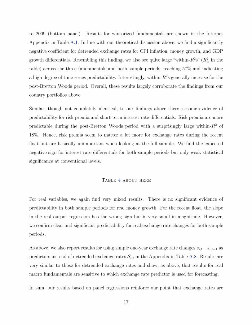
For real variables, we again find very mixed results. There is no significant evidence of

predictability in both sample periods for real money growth. For the recent float, the slope

in the real output regression has the wrong sign but is very small in magnitude. However,

we confirm clear and significant predictability for real exchange rate changes for both sample

periods.

As above, we also report results for using simple one-year exchange rate changes si,t−si,t−1 as

predictors instead of detrended exchange rates Si,t in the Appendix in Table A.8. Results are

very similar to those for detrended exchange rates and show, as above, that results for real

macro fundamentals are sensitive to which exchange rate predictor is used for forecasting.

In sum, our results based on panel regressions reinforce our point that exchange rates are

17

quite informative about nominal fundamentals, pointing towards a prominent role of nominal

fundamentals for the determination of exchange rates. Real fundamentals are harder to

forecast with exchange rates (results are more sensitive to the method employed) and, hence,

seem to matter less for exchange rate determination.

5. ADDITIONAL RESULTS AND ROBUSTNESS

5.1. Controlling for lagged fundamentals

Our empirical analysis so far shows that exchange rates (detrended exchange rates and ex-

change rate changes) predict future fundamentals in a way consistent with standard present-

value models of exchange rates. This predictive power of exchange rates for fundamentals

suggests that (expected) fundamentals drive exchange rates and, thus, supports the central

message of present-value models.

However, while our results are well in line with present-value reasoning, it is not inconceivable

that other mechanisms actually drive our results. To give a concrete example, consider

our finding above that exchange rates are strong predictors of nominal macro fundamentals

(CPI inflation, money growth, nominal GDP growth). This finding might be driven by the

importance of nominal factors for exchange rates plus standard present-value reasoning, but

it might as well be driven by the fact that countries with, e.g., higher lagged inflation tend

to have both depreciating exchange rates and higher inflation rates in the future. Under this

scenario, lagged inflation is informative about exchange rates as well as future inflation and

the predictive power of exchange rates for future inflation is spurious.

To examine this possibility and to provide robustness for our main result, we next present

tests which control for lagged macro fundamentals when assessing the predictive power of

exchange rates for fundamentals.15

15This is not a hypothesis coming directly from present-value models but seems nevertheless interestingsince it helps to clarify the link between exchange rates and fundamentals.

18

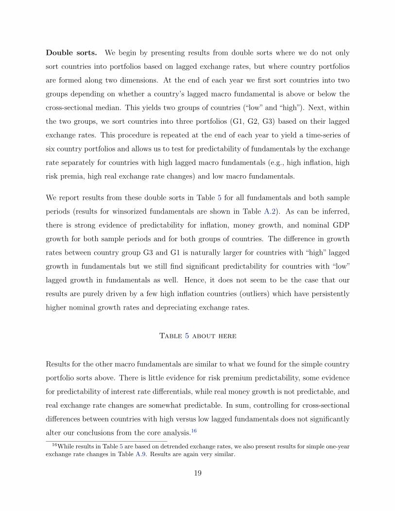
Double sorts. We begin by presenting results from double sorts where we do not only

sort countries into portfolios based on lagged exchange rates, but where country portfolios

are formed along two dimensions. At the end of each year we first sort countries into two

groups depending on whether a country’s lagged macro fundamental is above or below the

cross-sectional median. This yields two groups of countries (“low” and “high”). Next, within

the two groups, we sort countries into three portfolios (G1, G2, G3) based on their lagged

exchange rates. This procedure is repeated at the end of each year to yield a time-series of

six country portfolios and allows us to test for predictability of fundamentals by the exchange

rate separately for countries with high lagged macro fundamentals (e.g., high inflation, high

risk premia, high real exchange rate changes) and low macro fundamentals.

We report results from these double sorts in Table 5 for all fundamentals and both sample

periods (results for winsorized fundamentals are shown in Table A.2). As can be inferred,

there is strong evidence of predictability for inflation, money growth, and nominal GDP

growth for both sample periods and for both groups of countries. The difference in growth

rates between country group G3 and G1 is naturally larger for countries with “high” lagged

growth in fundamentals but we still find significant predictability for countries with “low”

lagged growth in fundamentals as well. Hence, it does not seem to be the case that our

results are purely driven by a few high inflation countries (outliers) which have persistently

higher nominal growth rates and depreciating exchange rates.

Table 5 about here

Results for the other macro fundamentals are similar to what we found for the simple country

portfolio sorts above. There is little evidence for risk premium predictability, some evidence

for predictability of interest rate differentials, while real money growth is not predictable, and

real exchange rate changes are somewhat predictable. In sum, controlling for cross-sectional

differences between countries with high versus low lagged fundamentals does not significantly

alter our conclusions from the core analysis.16

16While results in Table 5 are based on detrended exchange rates, we also present results for simple one-yearexchange rate changes in Table A.9. Results are again very similar.

19

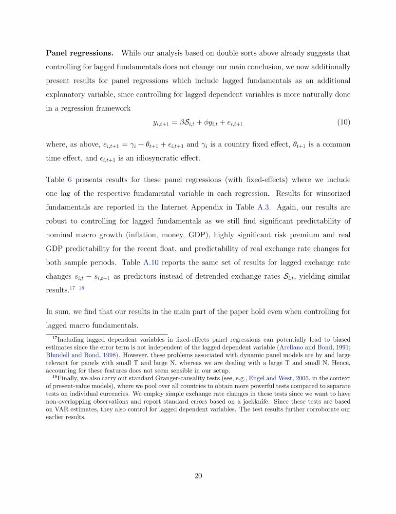
Panel regressions. While our analysis based on double sorts above already suggests that

controlling for lagged fundamentals does not change our main conclusion, we now additionally

present results for panel regressions which include lagged fundamentals as an additional

explanatory variable, since controlling for lagged dependent variables is more naturally done

in a regression framework

yi,t+1 = βSi,t + φyi,t + ei,t+1 (10)

where, as above, ei,t+1 = γi + θt+1 + εi,t+1 and γi is a country fixed effect, θt+1 is a common

time effect, and εi,t+1 is an idiosyncratic effect.

Table 6 presents results for these panel regressions (with fixed-effects) where we include

one lag of the respective fundamental variable in each regression. Results for winsorized

fundamentals are reported in the Internet Appendix in Table A.3. Again, our results are

robust to controlling for lagged fundamentals as we still find significant predictability of

nominal macro growth (inflation, money, GDP), highly significant risk premium and real

GDP predictability for the recent float, and predictability of real exchange rate changes for

both sample periods. Table A.10 reports the same set of results for lagged exchange rate

changes si,t − si,t−1 as predictors instead of detrended exchange rates Si,t, yielding similar

results.17 18

In sum, we find that our results in the main part of the paper hold even when controlling for

lagged macro fundamentals.

17Including lagged dependent variables in fixed-effects panel regressions can potentially lead to biasedestimates since the error term is not independent of the lagged dependent variable (Arellano and Bond, 1991;Blundell and Bond, 1998). However, these problems associated with dynamic panel models are by and largerelevant for panels with small T and large N, whereas we are dealing with a large T and small N. Hence,accounting for these features does not seem sensible in our setup.

18Finally, we also carry out standard Granger-causality tests (see, e.g., Engel and West, 2005, in the contextof present-value models), where we pool over all countries to obtain more powerful tests compared to separatetests on individual currencies. We employ simple exchange rate changes in these tests since we want to havenon-overlapping observations and report standard errors based on a jackknife. Since these tests are basedon VAR estimates, they also control for lagged dependent variables. The test results further corroborate ourearlier results.

20

5.2. Country sorts and longer forecast horizons

We finally present some results on predictability at longer horizons. Remember that the

present-value model discussed in Section 2 states that exchange rates forecast the sum of

future (discounted) fundamentals over long horizons and not just next year’s fundamen-

tals. Hence, in order to examine whether exchange rates depend on fundamentals at longer

horizons, we rely on our approach to form country portfolios as in the core analysis but

now examine the difference in growth rates between G4 and G1 at horizons ranging from

1, 2, ..., 10 after portfolio formation.

Figure 2 plots the (average) difference in growth rates for the first ten years after portfolio

formation for each macro fundamental and the sample period from 1909 to 1999 (since the

last 10-year forecast horizon starts in 2000).19 Shaded areas correspond to 95% confidence

intervals based on Newey and West (1987) standard errors.

Figure 2 about here

Results are relatively stable across time. There is a slight tendency for inflation, money

growth, and nominal GDP growth differentials to revert back to zero but this reversion is

not very strong.

Figure 3 shows the same exercise for the post-Bretton Woods period. Limiting the sample

period to 1974 – 1999 (again, the last ten years are only included as “forecast periods”)

naturally leads to wider confidence intervals for most fundamentals but also produces some

additional patterns. For example, the shaky evidence of risk premium predictability in Table 3

is largely confined to very short horizons of one year since at longer horizons there is significant

evidence of predictability. The opposite holds true for real exchange rate changes where

predictability dies out after about five to six years. Finally, we find that the theoretically

expected negative relationship between current exchange rates and future real money growth

19Note that the difference in growth rates for year 1 after portfolio formation can differ from the respectivevalues in Tables 2 and 3 due to the different sample periods.

21

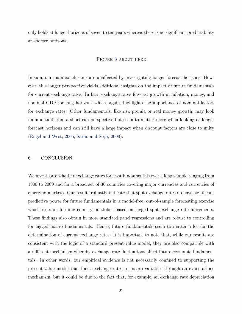
only holds at longer horizons of seven to ten years whereas there is no significant predictability

at shorter horizons.

Figure 3 about here

In sum, our main conclusions are unaffected by investigating longer forecast horizons. How-

ever, this longer perspective yields additional insights on the impact of future fundamentals

for current exchange rates. In fact, exchange rates forecast growth in inflation, money, and

nominal GDP for long horizons which, again, highlights the importance of nominal factors

for exchange rates. Other fundamentals, like risk premia or real money growth, may look

unimportant from a short-run perspective but seem to matter more when looking at longer

forecast horizons and can still have a large impact when discount factors are close to unity

(Engel and West, 2005; Sarno and Sojli, 2009).

6. CONCLUSION

We investigate whether exchange rates forecast fundamentals over a long sample ranging from

1900 to 2009 and for a broad set of 36 countries covering major currencies and currencies of

emerging markets. Our results robustly indicate that spot exchange rates do have significant

predictive power for future fundamentals in a model-free, out-of-sample forecasting exercise

which rests on forming country portfolios based on lagged spot exchange rate movements.

These findings also obtain in more standard panel regressions and are robust to controlling

for lagged macro fundamentals. Hence, future fundamentals seem to matter a lot for the

determination of current exchange rates. It is important to note that, while our results are

consistent with the logic of a standard present-value model, they are also compatible with

a different mechanism whereby exchange rate fluctuations affect future economic fundamen-

tals. In other words, our empirical evidence is not necessarily confined to supporting the

present-value model that links exchange rates to macro variables through an expectations

mechanism, but it could be due to the fact that, for example, an exchange rate depreciation

22

increases net exports and, hence, output. More generally, the fundamentals considered here

are endogenously determined together with exchange rates in equilibrium, which is consistent

with several alternative theories of exchange rate determination.

The results suggest that nominal macro fundamentals (CPI inflation, money growth, GDP

growth) are most robustly related to exchange rates. Risk premia (UIP deviations) and

real exchange rate changes only seem to matter during the recent float in the post-Bretton

Woods period and seem to play a minor role more generally. Real macro aggregates, such

as real output and real money, have no clear and meaningful relation to current exchange

rates and, hence, appear relatively unimportant for exchange rate determination. Overall,

we view the evidence in this paper as indicative of a meaningful link between exchange rates

and macro fundamentals, suggesting that nominal fundamentals are most important for the

determination of exchange rates whereas real factors matter only to a limited degree.

23

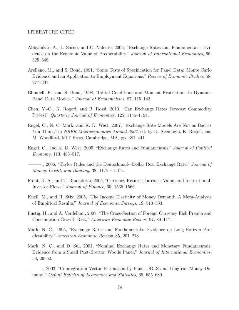
LITERATURE CITED

Abhyankar, A., L. Sarno, and G. Valente, 2005, “Exchange Rates and Fundamentals: Evi-

dence on the Economic Value of Predictability,” Journal of International Economics, 66,

325–348.

Arellano, M., and S. Bond, 1991, “Some Tests of Specification for Panel Data: Monte Carlo

Evidence and an Application to Employment Equations,”Review of Economic Studies, 58,

277–297.

Blundell, R., and S. Bond, 1998, “Initial Conditions and Moment Restrictions in Dynamic

Panel Data Models,” Journal of Econometrics, 87, 115–143.

Chen, Y.-C., K. Rogoff, and B. Rossi, 2010, “Can Exchange Rates Forecast Commodity

Prices?” Quarterly Journal of Economics, 125, 1145–1194.

Engel, C., N. C. Mark, and K. D. West, 2007, “Exchange Rate Models Are Not as Bad as

You Think,” in NBER Macroeconomics Annual 2007, ed. by D. Acemoglu, K. Rogoff, and

M. Woodford. MIT Press, Cambridge, MA, pp. 381–441.

Engel, C., and K. D. West, 2005, “Exchange Rates and Fundamentals,” Journal of Political

Economy, 113, 485–517.

, 2006, “Taylor Rules and the Deutschmark–Dollar Real Exchange Rate,” Journal of

Money, Credit, and Banking, 38, 1175 – 1194.

Froot, K. A., and T. Ramadorai, 2005, “Currency Returns, Intrinsic Value, and Institutional-

Investor Flows,” Journal of Finance, 60, 1535–1566.

Knell, M., and H. Stix, 2005, “The Income Elasticity of Money Demand: A Meta-Analysis

of Empirical Results,” Journal of Economic Surveys, 19, 513–533.

Lustig, H., and A. Verdelhan, 2007, “The Cross-Section of Foreign Currency Risk Premia and

Consumption Growth Risk,” American Economic Review, 97, 89–117.

Mark, N. C., 1995, “Exchange Rates and Fundamentals: Evidence on Long-Horizon Pre-

dictability,” American Economic Review, 85, 201–218.

Mark, N. C., and D. Sul, 2001, “Nominal Exchange Rates and Monetary Fundamentals:

Evidence from a Small Post-Bretton Woods Panel,” Journal of International Economics,

53, 29–52.

, 2003, “Cointegration Vector Estimation by Panel DOLS and Long-run Money De-

mand,” Oxford Bulletin of Economics and Statistics, 65, 655–680.

24

, 2012, “When Are Pooled Panel Data Regression Forecasts of Exchange Rates More

Accurate than the TimeSeries Regression Forecasts?” in Handbook of Exchange Rates, ed.

by J. James, I. Marsh, and L. Sarno. Wiley Publishing Inc., New Jersey, pp. 265–281.

Meese, R. A., and K. Rogoff, 1983, “Empirical Exchange Rate Models of the Seventies: Do

they fit out of Sample?” Journal of International Economics, 14, 3–24.

Menkhoff, L., L. Sarno, M. Schmeling, and A. Schrimpf, 2012a, “Carry Trades and Global

Foreign Exchange Volatility,” Journal of Finance, 67, 681–718.

, 2012b, “Currency Momentum Strategies,” Journal of Financial Economcis, 106,

660–684.

Newey, W. K., and K. D. West, 1987, “A Simple, Positive Semi-Definite, Heteroskedasticity

and Autocorrelation Consistent Covariance Matrix,” Econometrica, 55, 703–708.

Obstfeld, M., and K. Rogoff, 2000, “The Six Major Puzzles in International Macroeconomics:

Is there a Common Cause?” in NBER Macroeconomics Annual 2000, ed. by B. Bernanke,

and K. Rogoff. MIT Press, Cambridge.

Patton, A. J., and A. Timmermann, 2010, “Monotonicity in Asset Returns: New Tests with

Applications to the Term Structure, the CAPM and Portfolio Sorts,” Journal of Financial

Economics, 98, 605–625.

Politis, D. N., and J. P. Romano, 1994, “The Stationary Bootstrap,” Journal of the American

Statistical Association, 89, 1301–1313.

Sarno, L., and E. Sojli, 2009, “The Feeble Link Between Exchange Rates and Fundamentals:

Can We Blame the Discount Factor?” Journal of Money, Credit and Banking, 41, 437–442.

Stambaugh, R. F., 1999, “Predictive Regressions,” Journal of Financial Economics, 54, 375–

421.

25

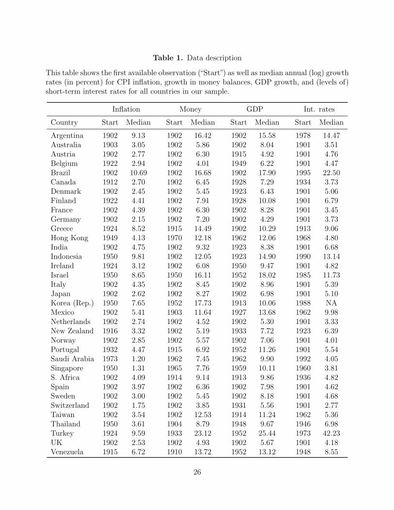
Table 1. Data description

This table shows the first available observation (“Start”) as well as median annual (log) growthrates (in percent) for CPI inflation, growth in money balances, GDP growth, and (levels of)short-term interest rates for all countries in our sample.

Inflation Money GDP Int. rates

Country Start Median Start Median Start Median Start Median

Argentina 1902 9.13 1902 16.42 1902 15.58 1978 14.47Australia 1903 3.05 1902 5.86 1902 8.04 1901 3.51Austria 1902 2.77 1902 6.30 1915 4.92 1901 4.76Belgium 1922 2.94 1902 4.01 1949 6.22 1901 4.47Brazil 1902 10.69 1902 16.68 1902 17.90 1995 22.50Canada 1912 2.70 1902 6.45 1928 7.29 1934 3.73Denmark 1902 2.45 1902 5.45 1923 6.43 1901 5.06Finland 1922 4.41 1902 7.91 1928 10.08 1901 6.79France 1902 4.39 1902 6.30 1902 8.28 1901 3.45Germany 1902 2.15 1902 7.20 1902 4.29 1901 3.73Greece 1924 8.52 1915 14.49 1902 10.29 1913 9.06Hong Kong 1949 4.13 1970 12.18 1962 12.06 1968 4.80India 1902 4.75 1902 9.32 1923 8.38 1901 6.68Indonesia 1950 9.81 1902 12.05 1923 14.90 1990 13.14Ireland 1924 3.12 1902 6.08 1950 9.47 1901 4.82Israel 1950 8.65 1950 16.11 1952 18.02 1985 11.73Italy 1902 4.35 1902 8.45 1902 8.96 1901 5.39Japan 1902 2.62 1902 8.27 1902 6.98 1901 5.10Korea (Rep.) 1950 7.65 1952 17.73 1913 10.06 1988 NAMexico 1902 5.41 1903 11.64 1927 13.68 1962 9.98Netherlands 1902 2.74 1902 4.52 1902 5.30 1901 3.33New Zealand 1916 3.32 1902 5.19 1933 7.72 1923 6.39Norway 1902 2.85 1902 5.57 1902 7.06 1901 4.01Portugal 1932 4.47 1915 6.92 1952 11.26 1901 5.54Saudi Arabia 1973 1.20 1962 7.45 1962 9.90 1992 4.05Singapore 1950 1.31 1965 7.76 1959 10.11 1960 3.81S. Africa 1902 4.09 1914 9.14 1913 9.86 1936 4.82Spain 1902 3.97 1902 6.36 1902 7.98 1901 4.62Sweden 1902 3.00 1902 5.45 1902 8.18 1901 4.68Switzerland 1902 1.75 1902 3.85 1931 5.56 1901 2.77Taiwan 1902 3.54 1902 12.53 1914 11.24 1962 5.36Thailand 1950 3.61 1904 8.79 1948 9.67 1946 6.98Turkey 1924 9.59 1933 23.12 1952 25.44 1973 42.23UK 1902 2.53 1902 4.93 1902 5.67 1901 4.18Venezuela 1915 6.72 1910 13.72 1952 13.12 1948 8.55

26

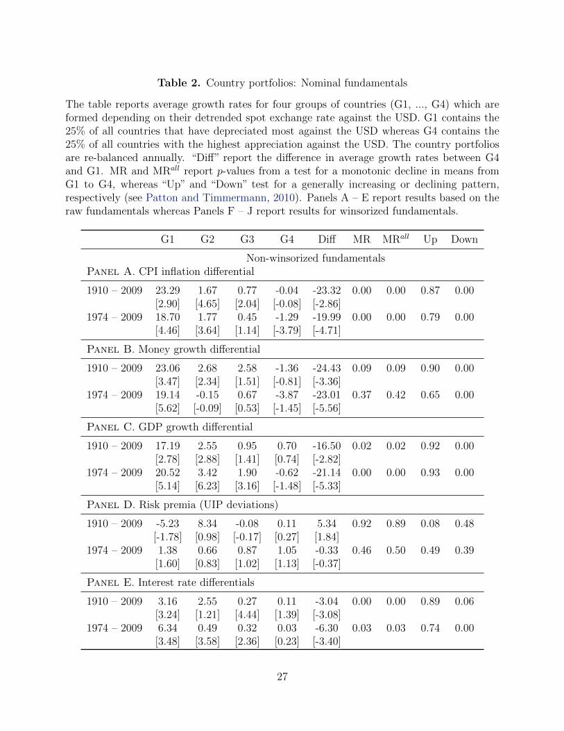
Table 2. Country portfolios: Nominal fundamentals

The table reports average growth rates for four groups of countries (G1, ..., G4) which areformed depending on their detrended spot exchange rate against the USD. G1 contains the25% of all countries that have depreciated most against the USD whereas G4 contains the25% of all countries with the highest appreciation against the USD. The country portfoliosare re-balanced annually. “Diff” report the difference in average growth rates between G4and G1. MR and MRall report p-values from a test for a monotonic decline in means fromG1 to G4, whereas “Up” and “Down” test for a generally increasing or declining pattern,respectively (see Patton and Timmermann, 2010). Panels A – E report results based on theraw fundamentals whereas Panels F – J report results for winsorized fundamentals.

G1 G2 G3 G4 Diff MR MRall Up Down

Non-winsorized fundamentalsPanel A. CPI inflation differential

1910 – 2009 23.29 1.67 0.77 -0.04 -23.32 0.00 0.00 0.87 0.00[2.90] [4.65] [2.04] [-0.08] [-2.86]

1974 – 2009 18.70 1.77 0.45 -1.29 -19.99 0.00 0.00 0.79 0.00[4.46] [3.64] [1.14] [-3.79] [-4.71]

Panel B. Money growth differential

1910 – 2009 23.06 2.68 2.58 -1.36 -24.43 0.09 0.09 0.90 0.00[3.47] [2.34] [1.51] [-0.81] [-3.36]

1974 – 2009 19.14 -0.15 0.67 -3.87 -23.01 0.37 0.42 0.65 0.00[5.62] [-0.09] [0.53] [-1.45] [-5.56]

Panel C. GDP growth differential

1910 – 2009 17.19 2.55 0.95 0.70 -16.50 0.02 0.02 0.92 0.00[2.78] [2.88] [1.41] [0.74] [-2.82]

1974 – 2009 20.52 3.42 1.90 -0.62 -21.14 0.00 0.00 0.93 0.00[5.14] [6.23] [3.16] [-1.48] [-5.33]

Panel D. Risk premia (UIP deviations)

1910 – 2009 -5.23 8.34 -0.08 0.11 5.34 0.92 0.89 0.08 0.48[-1.78] [0.98] [-0.17] [0.27] [1.84]

1974 – 2009 1.38 0.66 0.87 1.05 -0.33 0.46 0.50 0.49 0.39[1.60] [0.83] [1.02] [1.13] [-0.37]

Panel E. Interest rate differentials

1910 – 2009 3.16 2.55 0.27 0.11 -3.04 0.00 0.00 0.89 0.06[3.24] [1.21] [4.44] [1.39] [-3.08]

1974 – 2009 6.34 0.49 0.32 0.03 -6.30 0.03 0.03 0.74 0.00[3.48] [3.58] [2.36] [0.23] [-3.40]

27

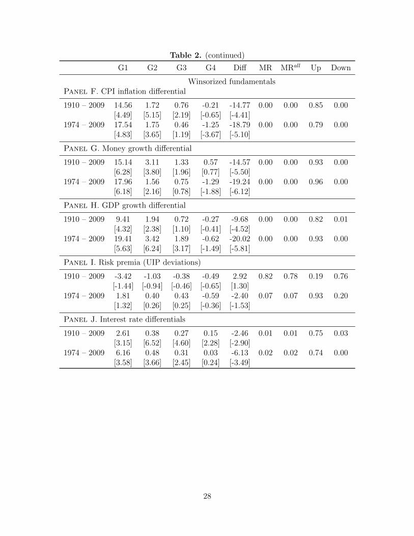
Table 2. (continued)


Winsorized fundamentalsPanel F. CPI inflation differential

1910 – 2009 14.56 1.72 0.76 -0.21 -14.77 0.00 0.00 0.85 0.00[4.49] [5.15] [2.19] [-0.65] [-4.41]

1974 – 2009 17.54 1.75 0.46 -1.25 -18.79 0.00 0.00 0.79 0.00[4.83] [3.65] [1.19] [-3.67] [-5.10]

Panel G. Money growth differential

1910 – 2009 15.14 3.11 1.33 0.57 -14.57 0.00 0.00 0.93 0.00[6.28] [3.80] [1.96] [0.77] [-5.50]

1974 – 2009 17.96 1.56 0.75 -1.29 -19.24 0.00 0.00 0.96 0.00[6.18] [2.16] [0.78] [-1.88] [-6.12]

Panel H. GDP growth differential

1910 – 2009 9.41 1.94 0.72 -0.27 -9.68 0.00 0.00 0.82 0.01[4.32] [2.38] [1.10] [-0.41] [-4.52]

1974 – 2009 19.41 3.42 1.89 -0.62 -20.02 0.00 0.00 0.93 0.00[5.63] [6.24] [3.17] [-1.49] [-5.81]

Panel I. Risk premia (UIP deviations)

1910 – 2009 -3.42 -1.03 -0.38 -0.49 2.92 0.82 0.78 0.19 0.76[-1.44] [-0.94] [-0.46] [-0.65] [1.30]

1974 – 2009 1.81 0.40 0.43 -0.59 -2.40 0.07 0.07 0.93 0.20[1.32] [0.26] [0.25] [-0.36] [-1.53]

Panel J. Interest rate differentials

1910 – 2009 2.61 0.38 0.27 0.15 -2.46 0.01 0.01 0.75 0.03[3.15] [6.52] [4.60] [2.28] [-2.90]

1974 – 2009 6.16 0.48 0.31 0.03 -6.13 0.02 0.02 0.74 0.00[3.58] [3.66] [2.45] [0.24] [-3.49]

28

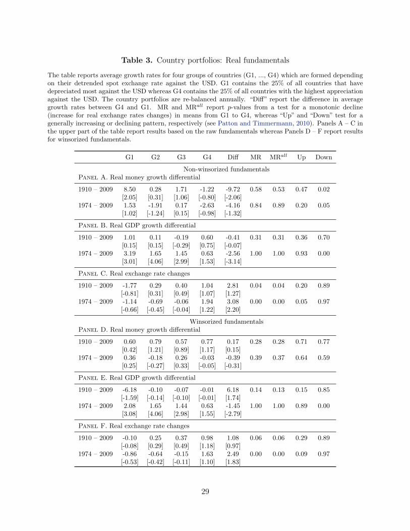
Table 3. Country portfolios: Real fundamentals

The table reports average growth rates for four groups of countries (G1, ..., G4) which are formed dependingon their detrended spot exchange rate against the USD. G1 contains the 25% of all countries that havedepreciated most against the USD whereas G4 contains the 25% of all countries with the highest appreciationagainst the USD. The country portfolios are re-balanced annually. “Diff” report the difference in averagegrowth rates between G4 and G1. MR and MRall report p-values from a test for a monotonic decline(increase for real exchange rates changes) in means from G1 to G4, whereas “Up” and “Down” test for agenerally increasing or declining pattern, respectively (see Patton and Timmermann, 2010). Panels A – C inthe upper part of the table report results based on the raw fundamentals whereas Panels D – F report resultsfor winsorized fundamentals.


Non-winsorized fundamentalsPanel A. Real money growth differential

1910 – 2009 8.50 0.28 1.71 -1.22 -9.72 0.58 0.53 0.47 0.02[2.05] [0.31] [1.06] [-0.80] [-2.06]

1974 – 2009 1.53 -1.91 0.17 -2.63 -4.16 0.84 0.89 0.20 0.05[1.02] [-1.24] [0.15] [-0.98] [-1.32]

Panel B. Real GDP growth differential

1910 – 2009 1.01 0.11 -0.19 0.60 -0.41 0.31 0.31 0.36 0.70[0.15] [0.15] [-0.29] [0.75] [-0.07]

1974 – 2009 3.19 1.65 1.45 0.63 -2.56 1.00 1.00 0.93 0.00[3.01] [4.06] [2.99] [1.53] [-3.14]

Panel C. Real exchange rate changes

1910 – 2009 -1.77 0.29 0.40 1.04 2.81 0.04 0.04 0.20 0.89[-0.81] [0.31] [0.49] [1.07] [1.27]

1974 – 2009 -1.14 -0.69 -0.06 1.94 3.08 0.00 0.00 0.05 0.97[-0.66] [-0.45] [-0.04] [1.22] [2.20]

Winsorized fundamentalsPanel D. Real money growth differential

1910 – 2009 0.60 0.79 0.57 0.77 0.17 0.28 0.28 0.71 0.77[0.42] [1.21] [0.89] [1.17] [0.15]

1974 – 2009 0.36 -0.18 0.26 -0.03 -0.39 0.39 0.37 0.64 0.59[0.25] [-0.27] [0.33] [-0.05] [-0.31]

Panel E. Real GDP growth differential

1910 – 2009 -6.18 -0.10 -0.07 -0.01 6.18 0.14 0.13 0.15 0.85[-1.59] [-0.14] [-0.10] [-0.01] [1.74]

1974 – 2009 2.08 1.65 1.44 0.63 -1.45 1.00 1.00 0.89 0.00[3.08] [4.06] [2.98] [1.55] [-2.79]

Panel F. Real exchange rate changes

1910 – 2009 -0.10 0.25 0.37 0.98 1.08 0.06 0.06 0.29 0.89[-0.08] [0.29] [0.49] [1.18] [0.97]

1974 – 2009 -0.86 -0.64 -0.15 1.63 2.49 0.00 0.00 0.09 0.97[-0.53] [-0.42] [-0.11] [1.10] [1.83]

29

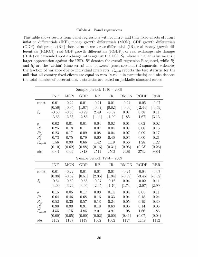
Table 4. Panel regressions

This table shows results from panel regressions with country- and time fixed-effects of futureinflation differentials (INF), money growth differentials (MON), GDP growth differentials(GDP), risk premia (RP) short-term interest rate differentials (IR), real money growth dif-ferentials (RMON), real GDP growth differentials (RGDP), or real exchange rate changes(RER) on detrended spot exchange rates against the USD St, where a higher value means alarger appreciation against the USD. R2 denotes the overall regression R-squared, while R2

w

and R2b are the “within” (time-series) and “between” (cross-sectional) R-squareds. % denotes

the fraction of variance due to individual intercepts, Fαi=0 reports the test statistic for thenull that all country fixed-effects are equal to zero (p-value in parenthesis) and obs denotesthe total number of observations. t-statistics are based on jackknife standard errors.

Sample period: 1910 – 2009

INF MON GDP RP IR RMON RGDP RER

const. 0.01 -0.22 0.01 -0.21 0.01 -0.24 -0.05 -0.07[0.56] [-0.85] [1.07] [-0.97] [0.82] [-0.90] [-2.44] [-3.59]

St -0.60 -0.53 -0.29 2.49 -0.07 0.07 0.38 0.11[-3.66] [-3.65] [-2.86] [1.11] [-1.90] [1.85] [1.67] [3.13]

% 0.02 0.01 0.01 0.04 0.02 0.01 0.02 0.02R2 0.25 0.18 0.11 0.07 0.04 0.07 0.08 0.16R2w 0.23 0.17 0.09 0.08 0.04 0.07 0.09 0.17

R2b 0.73 0.75 0.79 0.00 0.40 0.03 0.00 0.21

Fαi=0 1.56 0.90 0.66 1.42 1.19 0.56 1.28 1.22(0.10) (0.62) (0.88) (0.16) (0.31) (0.95) (0.23) (0.26)

obs 3004 3099 2818 2511 2503 2939 2732 3004



const. 0.01 -0.22 0.01 0.01 0.01 -0.24 -0.04 -0.07[0.38] [-0.82] [0.51] [2.35] [1.94] [-0.89] [-3.45] [-3.52]

St -0.54 -0.50 -0.56 -0.07 -0.16 0.04 -0.02 0.11[-4.00] [-3.24] [-3.96] [-2.95] [-1.76] [1.74] [-2.07] [2.99]

% 0.15 0.05 0.17 0.08 0.14 0.04 0.05 0.11R2 0.64 0.46 0.68 0.16 0.33 0.04 0.18 0.24R2w 0.52 0.30 0.57 0.18 0.24 0.05 0.19 0.30

R2b 0.90 0.90 0.91 0.18 0.63 0.05 0.14 0.05

Fαi=0 4.55 1.75 4.85 2.01 3.91 1.08 1.66 1.85(0.00) (0.05) (0.00) (0.02) (0.00) (0.41) (0.07) (0.04)

obs 1152 1137 1149 1062 1062 1137 1149 1152

30

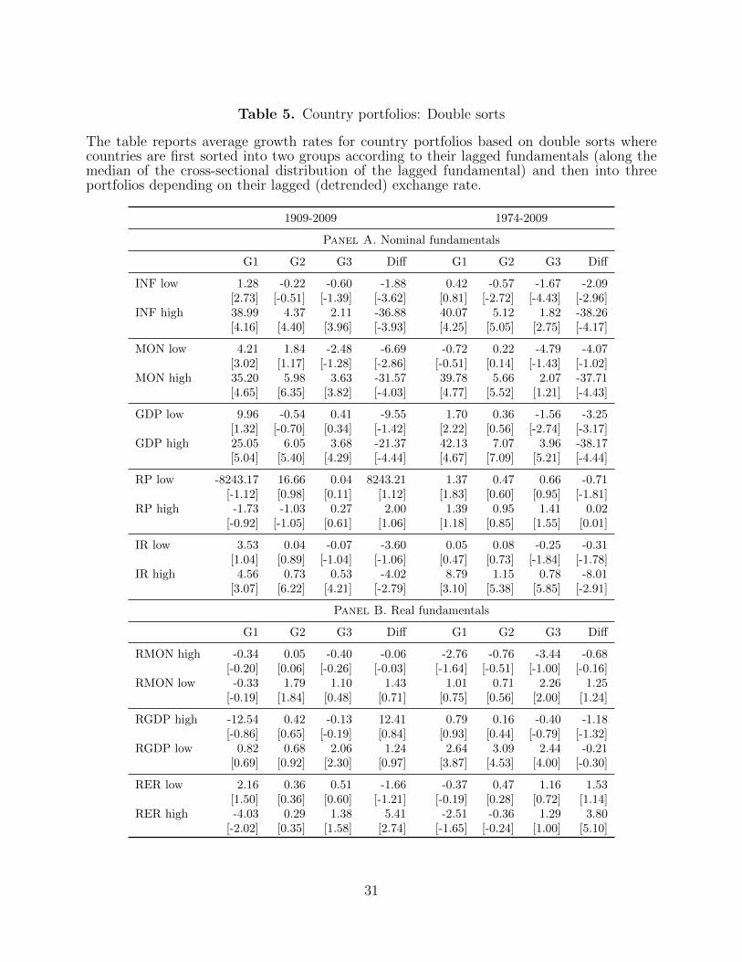
Table 5. Country portfolios: Double sorts

The table reports average growth rates for country portfolios based on double sorts wherecountries are first sorted into two groups according to their lagged fundamentals (along themedian of the cross-sectional distribution of the lagged fundamental) and then into threeportfolios depending on their lagged (detrended) exchange rate.

1909-2009 1974-2009

Panel A. Nominal fundamentals

G1 G2 G3 Diff G1 G2 G3 Diff

INF low 1.28 -0.22 -0.60 -1.88 0.42 -0.57 -1.67 -2.09[2.73] [-0.51] [-1.39] [-3.62] [0.81] [-2.72] [-4.43] [-2.96]

INF high 38.99 4.37 2.11 -36.88 40.07 5.12 1.82 -38.26[4.16] [4.40] [3.96] [-3.93] [4.25] [5.05] [2.75] [-4.17]

MON low 4.21 1.84 -2.48 -6.69 -0.72 0.22 -4.79 -4.07[3.02] [1.17] [-1.28] [-2.86] [-0.51] [0.14] [-1.43] [-1.02]

MON high 35.20 5.98 3.63 -31.57 39.78 5.66 2.07 -37.71[4.65] [6.35] [3.82] [-4.03] [4.77] [5.52] [1.21] [-4.43]

GDP low 9.96 -0.54 0.41 -9.55 1.70 0.36 -1.56 -3.25[1.32] [-0.70] [0.34] [-1.42] [2.22] [0.56] [-2.74] [-3.17]

GDP high 25.05 6.05 3.68 -21.37 42.13 7.07 3.96 -38.17[5.04] [5.40] [4.29] [-4.44] [4.67] [7.09] [5.21] [-4.44]

RP low -8243.17 16.66 0.04 8243.21 1.37 0.47 0.66 -0.71[-1.12] [0.98] [0.11] [1.12] [1.83] [0.60] [0.95] [-1.81]

RP high -1.73 -1.03 0.27 2.00 1.39 0.95 1.41 0.02[-0.92] [-1.05] [0.61] [1.06] [1.18] [0.85] [1.55] [0.01]

IR low 3.53 0.04 -0.07 -3.60 0.05 0.08 -0.25 -0.31[1.04] [0.89] [-1.04] [-1.06] [0.47] [0.73] [-1.84] [-1.78]

IR high 4.56 0.73 0.53 -4.02 8.79 1.15 0.78 -8.01[3.07] [6.22] [4.21] [-2.79] [3.10] [5.38] [5.85] [-2.91]

Panel B. Real fundamentals


RMON high -0.34 0.05 -0.40 -0.06 -2.76 -0.76 -3.44 -0.68[-0.20] [0.06] [-0.26] [-0.03] [-1.64] [-0.51] [-1.00] [-0.16]

RMON low -0.33 1.79 1.10 1.43 1.01 0.71 2.26 1.25[-0.19] [1.84] [0.48] [0.71] [0.75] [0.56] [2.00] [1.24]

RGDP high -12.54 0.42 -0.13 12.41 0.79 0.16 -0.40 -1.18[-0.86] [0.65] [-0.19] [0.84] [0.93] [0.44] [-0.79] [-1.32]

RGDP low 0.82 0.68 2.06 1.24 2.64 3.09 2.44 -0.21[0.69] [0.92] [2.30] [0.97] [3.87] [4.53] [4.00] [-0.30]

RER low 2.16 0.36 0.51 -1.66 -0.37 0.47 1.16 1.53[1.50] [0.36] [0.60] [-1.21] [-0.19] [0.28] [0.72] [1.14]

RER high -4.03 0.29 1.38 5.41 -2.51 -0.36 1.29 3.80[-2.02] [0.35] [1.58] [2.74] [-1.65] [-0.24] [1.00] [5.10]

31

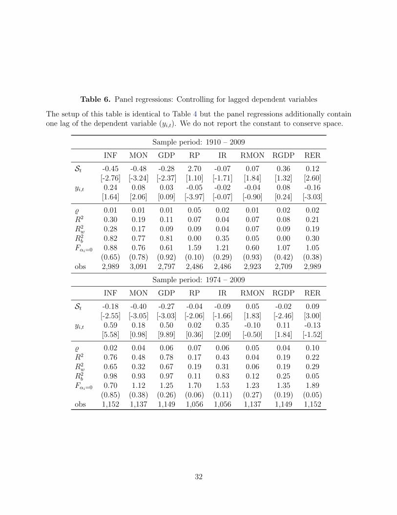
Table 6. Panel regressions: Controlling for lagged dependent variables

The setup of this table is identical to Table 4 but the panel regressions additionally containone lag of the dependent variable (yi,t). We do not report the constant to conserve space.



St -0.45 -0.48 -0.28 2.70 -0.07 0.07 0.36 0.12[-2.76] [-3.24] [-2.37] [1.10] [-1.71] [1.84] [1.32] [2.60]

yi,t 0.24 0.08 0.03 -0.05 -0.02 -0.04 0.08 -0.16[1.64] [2.06] [0.09] [-3.97] [-0.07] [-0.90] [0.24] [-3.03]

% 0.01 0.01 0.01 0.05 0.02 0.01 0.02 0.02R2 0.30 0.19 0.11 0.07 0.04 0.07 0.08 0.21R2w 0.28 0.17 0.09 0.09 0.04 0.07 0.09 0.19

R2b 0.82 0.77 0.81 0.00 0.35 0.05 0.00 0.30

Fαi=0 0.88 0.76 0.61 1.59 1.21 0.60 1.07 1.05(0.65) (0.78) (0.92) (0.10) (0.29) (0.93) (0.42) (0.38)

obs 2,989 3,091 2,797 2,486 2,486 2,923 2,709 2,989



St -0.18 -0.40 -0.27 -0.04 -0.09 0.05 -0.02 0.09[-2.55] [-3.05] [-3.03] [-2.06] [-1.66] [1.83] [-2.46] [3.00]

yi,t 0.59 0.18 0.50 0.02 0.35 -0.10 0.11 -0.13[5.58] [0.98] [9.89] [0.36] [2.09] [-0.50] [1.84] [-1.52]

% 0.02 0.04 0.06 0.07 0.06 0.05 0.04 0.10R2 0.76 0.48 0.78 0.17 0.43 0.04 0.19 0.22R2w 0.65 0.32 0.67 0.19 0.31 0.06 0.19 0.29

R2b 0.98 0.93 0.97 0.11 0.83 0.12 0.25 0.05

Fαi=0 0.70 1.12 1.25 1.70 1.53 1.23 1.35 1.89(0.85) (0.38) (0.26) (0.06) (0.11) (0.27) (0.19) (0.05)

obs 1,152 1,137 1,149 1,056 1,056 1,137 1,149 1,152

32

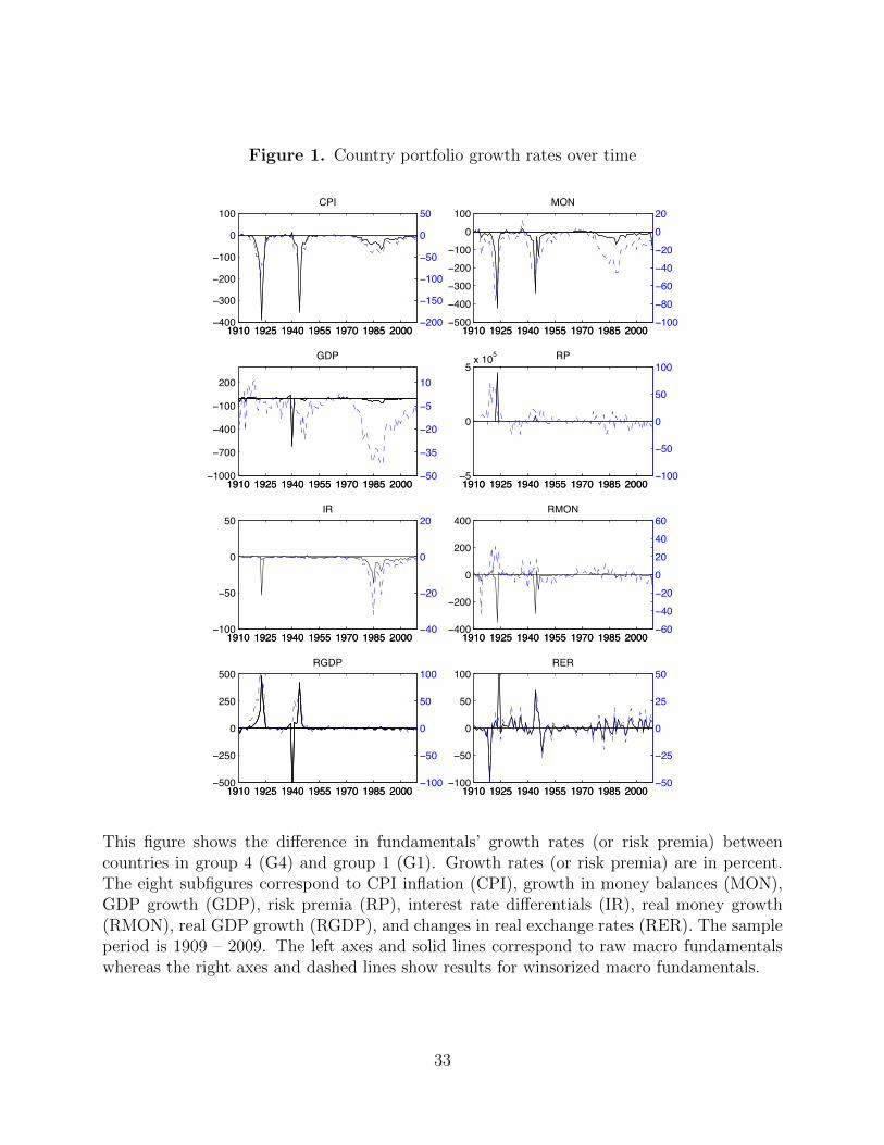
Figure 1. Country portfolio growth rates over time

1910 1925 1940 1955 1970 1985 2000−400

−300

−200

−100

0

100CPI

1910 1925 1940 1955 1970 1985 2000−500−400−300−200−100

0100

MON

1910 1925 1940 1955 1970 1985 2000−1000

−700

−400

−100

200

GDP

1910 1925 1940 1955 1970 1985 2000−5

0

5x 105 RP

1910 1925 1940 1955 1970 1985 2000−100

−50

0

50IR

1910 1925 1940 1955 1970 1985 2000−40

−20

0

20

1910 1925 1940 1955 1970 1985 2000−400

−200

0

200

400RMON

1910 1925 1940 1955 1970 1985 2000−60−40−200204060

1910 1925 1940 1955 1970 1985 2000−500

−250

0

250

500RGDP

1910 1925 1940 1955 1970 1985 2000−100

−50

0

50

100RER

1910 1925 1940 1955 1970 1985 2000−100

−50

0

50

100

1910 1925 1940 1955 1970 1985 2000−50

−25

0

25

50

1910 1925 1940 1955 1970 1985 2000−100−80−60−40−20020

1910 1925 1940 1955 1970 1985 2000−50

−35

−20

−5

10

1910 1925 1940 1955 1970 1985 2000−100

−50

0

50

100

1910 1925 1940 1955 1970 1985 2000−200

−150

−100

−50

0

50

This figure shows the difference in fundamentals’ growth rates (or risk premia) betweencountries in group 4 (G4) and group 1 (G1). Growth rates (or risk premia) are in percent.The eight subfigures correspond to CPI inflation (CPI), growth in money balances (MON),GDP growth (GDP), risk premia (RP), interest rate differentials (IR), real money growth(RMON), real GDP growth (RGDP), and changes in real exchange rates (RER). The sampleperiod is 1909 – 2009. The left axes and solid lines correspond to raw macro fundamentalswhereas the right axes and dashed lines show results for winsorized macro fundamentals.

33

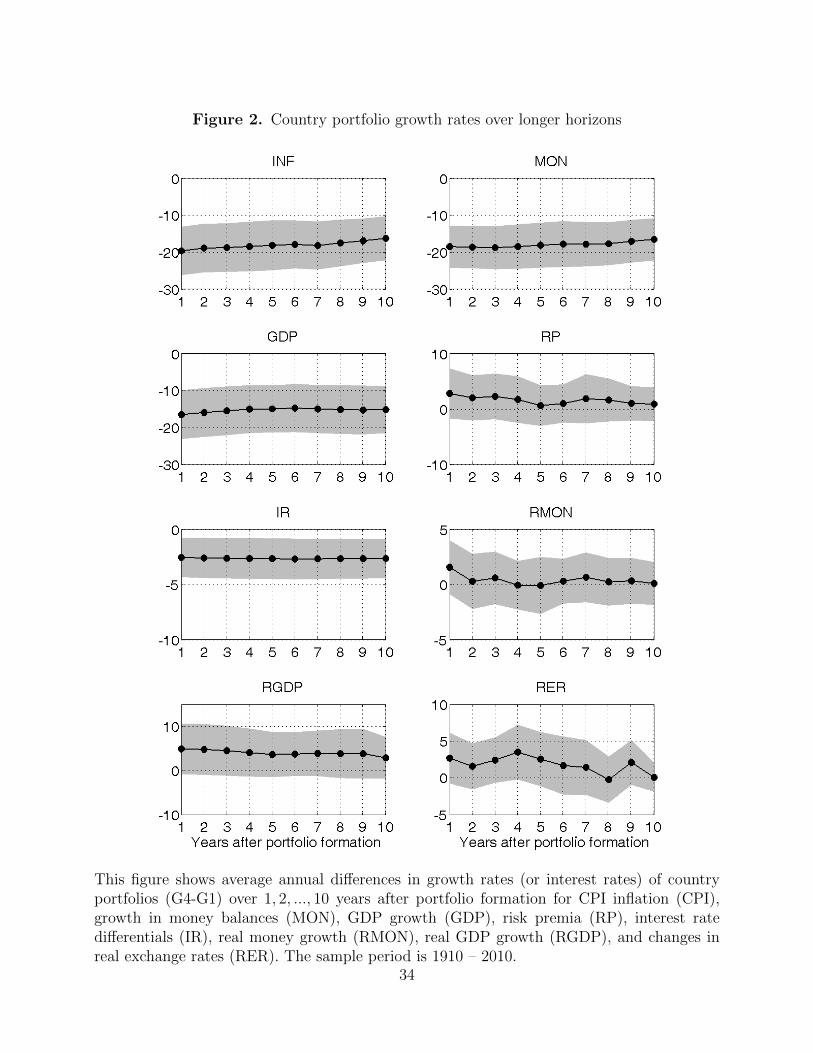
Figure 2. Country portfolio growth rates over longer horizons

This figure shows average annual differences in growth rates (or interest rates) of countryportfolios (G4-G1) over 1, 2, ..., 10 years after portfolio formation for CPI inflation (CPI),growth in money balances (MON), GDP growth (GDP), risk premia (RP), interest ratedifferentials (IR), real money growth (RMON), real GDP growth (RGDP), and changes inreal exchange rates (RER). The sample period is 1910 – 2010.

34

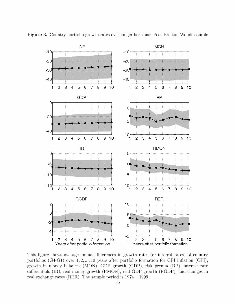
Figure 3. Country portfolio growth rates over longer horizons: Post-Bretton Woods sample

This figure shows average annual differences in growth rates (or interest rates) of countryportfolios (G4-G1) over 1, 2, ..., 10 years after portfolio formation for CPI inflation (CPI),growth in money balances (MON), GDP growth (GDP), risk premia (RP), interest ratedifferentials (IR), real money growth (RMON), real GDP growth (RGDP), and changes inreal exchange rates (RER). The sample period is 1974 – 1999.

35

Internet Appendix for

Which Fundamentals Drive Exchange Rates?

A Cross-Sectional Perspective

36

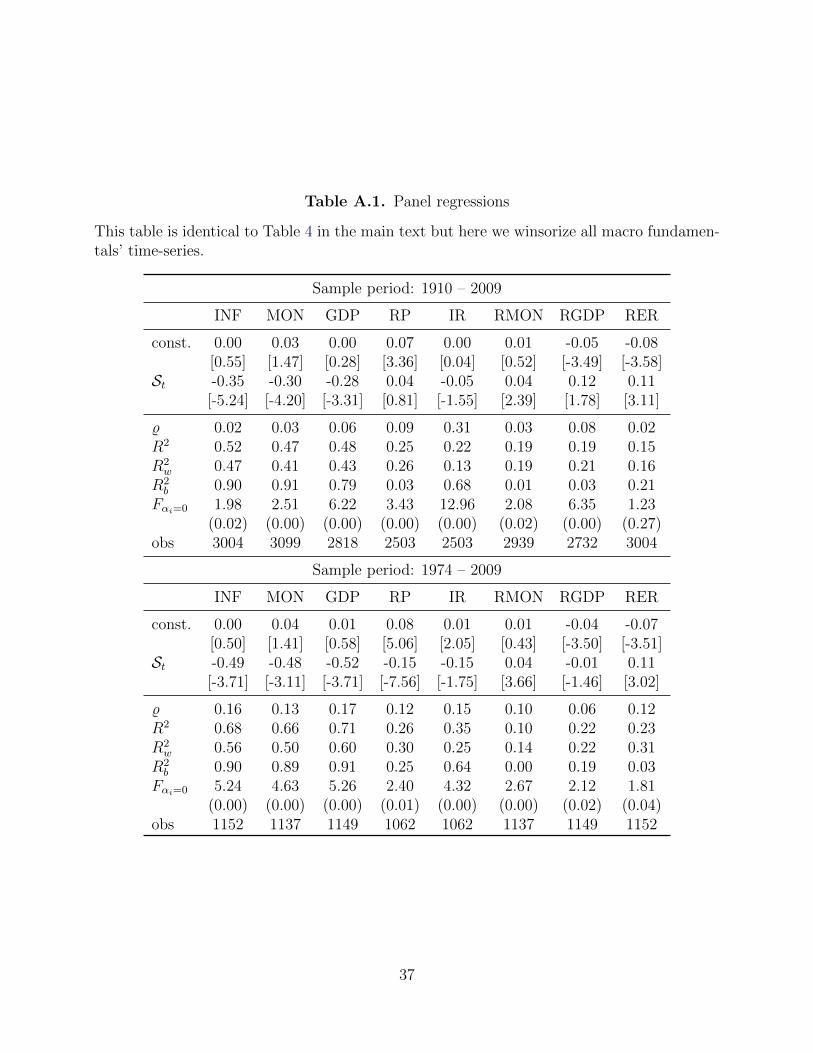
Table A.1. Panel regressions

This table is identical to Table 4 in the main text but here we winsorize all macro fundamen-tals’ time-series.



const. 0.00 0.03 0.00 0.07 0.00 0.01 -0.05 -0.08[0.55] [1.47] [0.28] [3.36] [0.04] [0.52] [-3.49] [-3.58]

St -0.35 -0.30 -0.28 0.04 -0.05 0.04 0.12 0.11[-5.24] [-4.20] [-3.31] [0.81] [-1.55] [2.39] [1.78] [3.11]

% 0.02 0.03 0.06 0.09 0.31 0.03 0.08 0.02R2 0.52 0.47 0.48 0.25 0.22 0.19 0.19 0.15R2w 0.47 0.41 0.43 0.26 0.13 0.19 0.21 0.16

R2b 0.90 0.91 0.79 0.03 0.68 0.01 0.03 0.21

Fαi=0 1.98 2.51 6.22 3.43 12.96 2.08 6.35 1.23(0.02) (0.00) (0.00) (0.00) (0.00) (0.02) (0.00) (0.27)

obs 3004 3099 2818 2503 2503 2939 2732 3004



const. 0.00 0.04 0.01 0.08 0.01 0.01 -0.04 -0.07[0.50] [1.41] [0.58] [5.06] [2.05] [0.43] [-3.50] [-3.51]

St -0.49 -0.48 -0.52 -0.15 -0.15 0.04 -0.01 0.11[-3.71] [-3.11] [-3.71] [-7.56] [-1.75] [3.66] [-1.46] [3.02]

% 0.16 0.13 0.17 0.12 0.15 0.10 0.06 0.12R2 0.68 0.66 0.71 0.26 0.35 0.10 0.22 0.23R2w 0.56 0.50 0.60 0.30 0.25 0.14 0.22 0.31

R2b 0.90 0.89 0.91 0.25 0.64 0.00 0.19 0.03

Fαi=0 5.24 4.63 5.26 2.40 4.32 2.67 2.12 1.81(0.00) (0.00) (0.00) (0.01) (0.00) (0.00) (0.02) (0.04)

obs 1152 1137 1149 1062 1062 1137 1149 1152

37

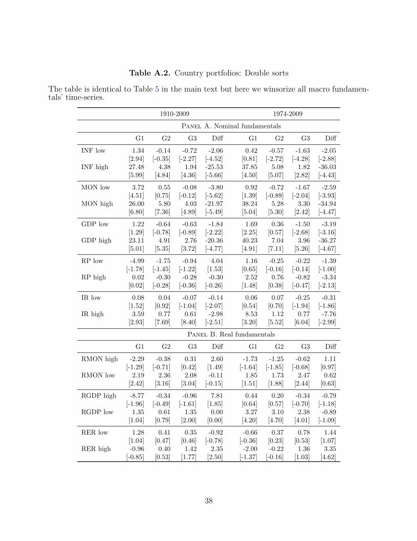
Table A.2. Country portfolios: Double sorts

The table is identical to Table 5 in the main text but here we winsorize all macro fundamen-tals’ time-series.

1910-2009 1974-2009



INF low 1.34 -0.14 -0.72 -2.06 0.42 -0.57 -1.63 -2.05[2.94] [-0.35] [-2.27] [-4.52] [0.81] [-2.72] [-4.28] [-2.88]

INF high 27.48 4.38 1.94 -25.53 37.85 5.08 1.82 -36.03[5.99] [4.84] [4.36] [-5.66] [4.50] [5.07] [2.82] [-4.43]

MON low 3.72 0.55 -0.08 -3.80 0.92 -0.72 -1.67 -2.59[4.51] [0.75] [-0.12] [-5.62] [1.39] [-0.89] [-2.04] [-3.93]

MON high 26.00 5.80 4.03 -21.97 38.24 5.28 3.30 -34.94[6.80] [7.36] [4.89] [-5.49] [5.04] [5.30] [2.42] [-4.47]

GDP low 1.22 -0.64 -0.63 -1.84 1.69 0.36 -1.50 -3.19[1.29] [-0.78] [-0.89] [-2.22] [2.25] [0.57] [-2.68] [-3.16]

GDP high 23.11 4.91 2.76 -20.36 40.23 7.04 3.96 -36.27[5.01] [5.35] [3.72] [-4.77] [4.91] [7.11] [5.26] [-4.67]

RP low -4.99 -1.75 -0.94 4.04 1.16 -0.25 -0.22 -1.39[-1.78] [-1.45] [-1.22] [1.53] [0.65] [-0.16] [-0.14] [-1.00]

RP high 0.02 -0.30 -0.28 -0.30 2.52 0.76 -0.82 -3.34[0.02] [-0.28] [-0.36] [-0.26] [1.48] [0.38] [-0.47] [-2.13]

IR low 0.08 0.04 -0.07 -0.14 0.06 0.07 -0.25 -0.31[1.52] [0.92] [-1.04] [-2.07] [0.54] [0.70] [-1.94] [-1.86]

IR high 3.59 0.77 0.61 -2.98 8.53 1.12 0.77 -7.76[2.93] [7.69] [8.40] [-2.51] [3.20] [5.52] [6.04] [-2.99]



RMON high -2.29 -0.38 0.31 2.60 -1.73 -1.25 -0.62 1.11[-1.29] [-0.71] [0.42] [1.49] [-1.64] [-1.85] [-0.68] [0.97]

RMON low 2.19 2.36 2.08 -0.11 1.85 1.73 2.47 0.62[2.42] [3.16] [3.04] [-0.15] [1.51] [1.88] [2.44] [0.63]

RGDP high -8.77 -0.34 -0.96 7.81 0.44 0.20 -0.34 -0.79[-1.96] [-0.49] [-1.61] [1.85] [0.64] [0.57] [-0.70] [-1.18]

RGDP low 1.35 0.61 1.35 0.00 3.27 3.10 2.38 -0.89[1.04] [0.79] [2.00] [0.00] [4.20] [4.70] [4.01] [-1.09]

RER low 1.28 0.41 0.35 -0.92 -0.66 0.37 0.78 1.44[1.04] [0.47] [0.46] [-0.78] [-0.36] [0.23] [0.53] [1.07]

RER high -0.96 0.40 1.42 2.35 -2.00 -0.22 1.36 3.35[-0.85] [0.53] [1.77] [2.50] [-1.37] [-0.16] [1.03] [4.62]

38

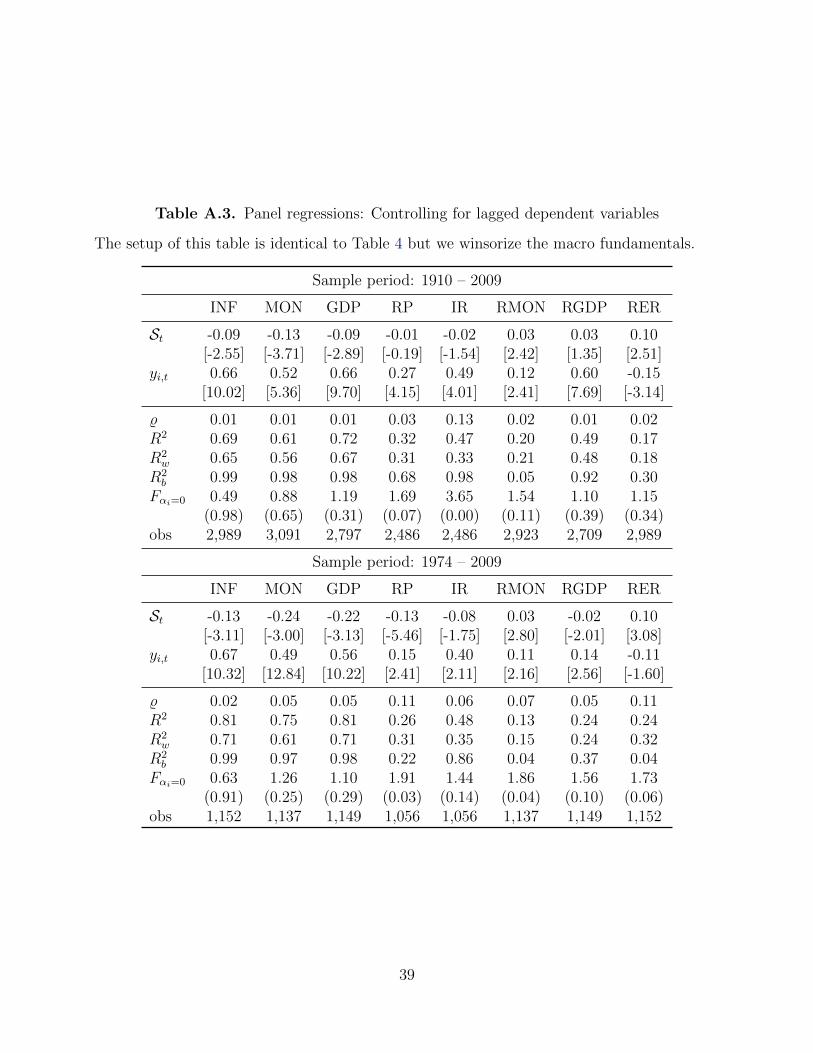
Table A.3. Panel regressions: Controlling for lagged dependent variables

The setup of this table is identical to Table 4 but we winsorize the macro fundamentals.



St -0.09 -0.13 -0.09 -0.01 -0.02 0.03 0.03 0.10[-2.55] [-3.71] [-2.89] [-0.19] [-1.54] [2.42] [1.35] [2.51]

yi,t 0.66 0.52 0.66 0.27 0.49 0.12 0.60 -0.15[10.02] [5.36] [9.70] [4.15] [4.01] [2.41] [7.69] [-3.14]

% 0.01 0.01 0.01 0.03 0.13 0.02 0.01 0.02R2 0.69 0.61 0.72 0.32 0.47 0.20 0.49 0.17R2w 0.65 0.56 0.67 0.31 0.33 0.21 0.48 0.18

R2b 0.99 0.98 0.98 0.68 0.98 0.05 0.92 0.30

Fαi=0 0.49 0.88 1.19 1.69 3.65 1.54 1.10 1.15(0.98) (0.65) (0.31) (0.07) (0.00) (0.11) (0.39) (0.34)

obs 2,989 3,091 2,797 2,486 2,486 2,923 2,709 2,989



St -0.13 -0.24 -0.22 -0.13 -0.08 0.03 -0.02 0.10[-3.11] [-3.00] [-3.13] [-5.46] [-1.75] [2.80] [-2.01] [3.08]

yi,t 0.67 0.49 0.56 0.15 0.40 0.11 0.14 -0.11[10.32] [12.84] [10.22] [2.41] [2.11] [2.16] [2.56] [-1.60]

% 0.02 0.05 0.05 0.11 0.06 0.07 0.05 0.11R2 0.81 0.75 0.81 0.26 0.48 0.13 0.24 0.24R2w 0.71 0.61 0.71 0.31 0.35 0.15 0.24 0.32

R2b 0.99 0.97 0.98 0.22 0.86 0.04 0.37 0.04

Fαi=0 0.63 1.26 1.10 1.91 1.44 1.86 1.56 1.73(0.91) (0.25) (0.29) (0.03) (0.14) (0.04) (0.10) (0.06)

obs 1,152 1,137 1,149 1,056 1,056 1,137 1,149 1,152

39

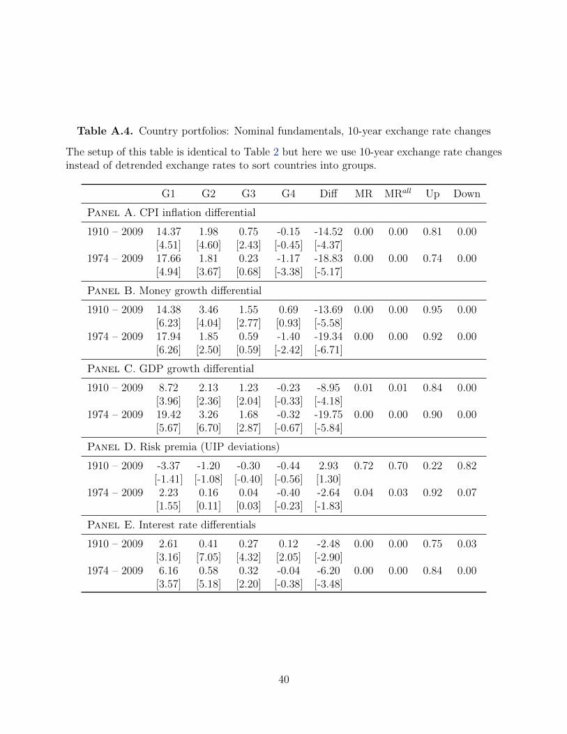
Table A.4. Country portfolios: Nominal fundamentals, 10-year exchange rate changes

The setup of this table is identical to Table 2 but here we use 10-year exchange rate changesinstead of detrended exchange rates to sort countries into groups.


Panel A. CPI inflation differential

1910 – 2009 14.37 1.98 0.75 -0.15 -14.52 0.00 0.00 0.81 0.00[4.51] [4.60] [2.43] [-0.45] [-4.37]

1974 – 2009 17.66 1.81 0.23 -1.17 -18.83 0.00 0.00 0.74 0.00[4.94] [3.67] [0.68] [-3.38] [-5.17]


1910 – 2009 14.38 3.46 1.55 0.69 -13.69 0.00 0.00 0.95 0.00[6.23] [4.04] [2.77] [0.93] [-5.58]

1974 – 2009 17.94 1.85 0.59 -1.40 -19.34 0.00 0.00 0.92 0.00[6.26] [2.50] [0.59] [-2.42] [-6.71]


1910 – 2009 8.72 2.13 1.23 -0.23 -8.95 0.01 0.01 0.84 0.00[3.96] [2.36] [2.04] [-0.33] [-4.18]

1974 – 2009 19.42 3.26 1.68 -0.32 -19.75 0.00 0.00 0.90 0.00[5.67] [6.70] [2.87] [-0.67] [-5.84]


1910 – 2009 -3.37 -1.20 -0.30 -0.44 2.93 0.72 0.70 0.22 0.82[-1.41] [-1.08] [-0.40] [-0.56] [1.30]

1974 – 2009 2.23 0.16 0.04 -0.40 -2.64 0.04 0.03 0.92 0.07[1.55] [0.11] [0.03] [-0.23] [-1.83]


1910 – 2009 2.61 0.41 0.27 0.12 -2.48 0.00 0.00 0.75 0.03[3.16] [7.05] [4.32] [2.05] [-2.90]

1974 – 2009 6.16 0.58 0.32 -0.04 -6.20 0.00 0.00 0.84 0.00[3.57] [5.18] [2.20] [-0.38] [-3.48]

40

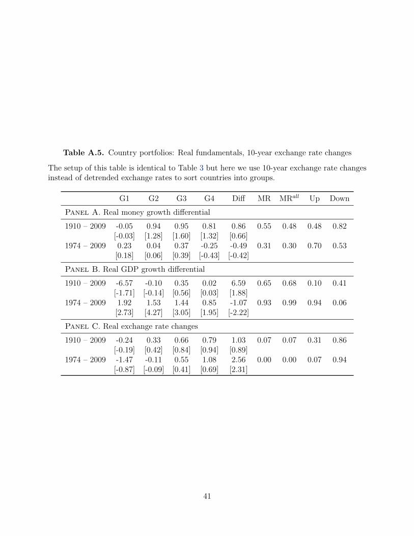
Table A.5. Country portfolios: Real fundamentals, 10-year exchange rate changes

The setup of this table is identical to Table 3 but here we use 10-year exchange rate changesinstead of detrended exchange rates to sort countries into groups.


Panel A. Real money growth differential

1910 – 2009 -0.05 0.94 0.95 0.81 0.86 0.55 0.48 0.48 0.82[-0.03] [1.28] [1.60] [1.32] [0.66]

1974 – 2009 0.23 0.04 0.37 -0.25 -0.49 0.31 0.30 0.70 0.53[0.18] [0.06] [0.39] [-0.43] [-0.42]


1910 – 2009 -6.57 -0.10 0.35 0.02 6.59 0.65 0.68 0.10 0.41[-1.71] [-0.14] [0.56] [0.03] [1.88]

1974 – 2009 1.92 1.53 1.44 0.85 -1.07 0.93 0.99 0.94 0.06[2.73] [4.27] [3.05] [1.95] [-2.22]


1910 – 2009 -0.24 0.33 0.66 0.79 1.03 0.07 0.07 0.31 0.86[-0.19] [0.42] [0.84] [0.94] [0.89]

1974 – 2009 -1.47 -0.11 0.55 1.08 2.56 0.00 0.00 0.07 0.94[-0.87] [-0.09] [0.41] [0.69] [2.31]

41

Table A.6. Country portfolios: Nominal fundamentals and simple exchange rate changes

The setup of this table is identical to Table 2 but here we sort countries into portfolios basedon simple (annual) exchange rate changes (instead of detrended spot exchange rates).


Panel A. CPI inflation differential

1910 – 2009 12.06 1.78 1.08 0.96 -11.09 0.06 0.06 0.87 0.00[4.17] [5.21] [3.02] [2.83] [-3.88]

1974 – 2009 14.82 2.27 1.28 0.07 -14.75 0.00 0.00 0.89 0.00[4.30] [5.55] [2.67] [0.22] [-4.38]


1910 – 2009 11.12 3.43 2.46 2.40 -8.72 0.07 0.07 0.90 0.00[5.18] [4.67] [3.43] [2.98] [-3.75]

1974 – 2009 13.63 2.55 1.43 1.54 -12.10 0.08 0.08 0.92 0.00[4.56] [2.79] [1.62] [2.43] [-3.62]


1910 – 2009 7.22 2.60 0.37 0.97 -6.24 0.52 0.47 0.51 0.00[3.65] [3.61] [0.45] [1.41] [-3.33]

1974 – 2009 16.03 4.37 2.41 1.34 -14.70 0.00 0.00 0.96 0.00[4.73] [7.44] [3.67] [2.84] [-4.41]


1910 – 2009 -3.10 -0.93 0.46 -0.82 2.28 0.87 0.90 0.07 0.05[-1.61] [-0.91] [0.56] [-0.86] [1.59]

1974 – 2009 0.85 0.70 0.71 -0.05 -0.90 0.09 0.09 0.91 0.36[0.70] [0.45] [0.42] [-0.03] [-0.69]


1910 – 2009 2.22 0.46 0.37 0.32 -1.91 0.00 0.00 0.93 0.05[2.80] [7.75] [5.93] [5.58] [-2.41]

1974 – 2009 5.38 0.67 0.59 0.39 -4.99 0.00 0.00 0.92 0.02[3.07] [7.78] [5.57] [3.39] [-2.82]

42

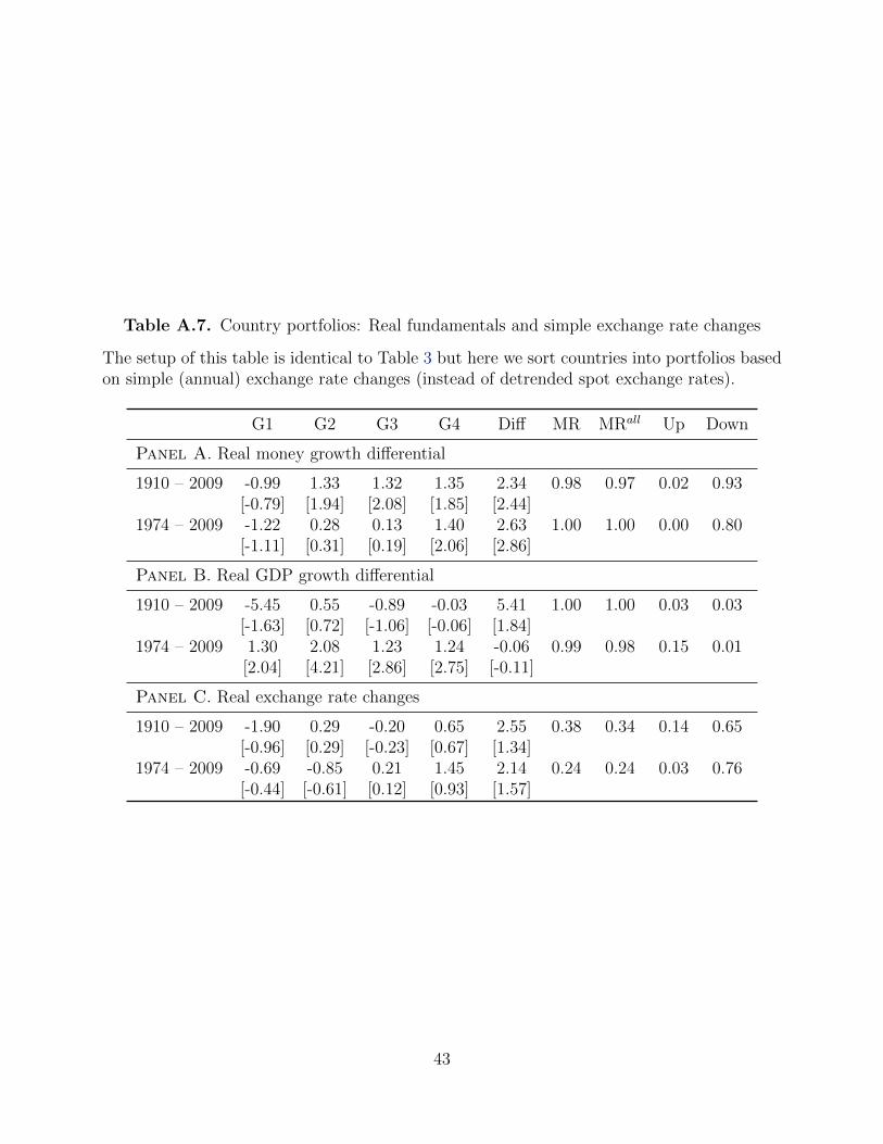
Table A.7. Country portfolios: Real fundamentals and simple exchange rate changes

The setup of this table is identical to Table 3 but here we sort countries into portfolios basedon simple (annual) exchange rate changes (instead of detrended spot exchange rates).


Panel A. Real money growth differential

1910 – 2009 -0.99 1.33 1.32 1.35 2.34 0.98 0.97 0.02 0.93[-0.79] [1.94] [2.08] [1.85] [2.44]

1974 – 2009 -1.22 0.28 0.13 1.40 2.63 1.00 1.00 0.00 0.80[-1.11] [0.31] [0.19] [2.06] [2.86]


1910 – 2009 -5.45 0.55 -0.89 -0.03 5.41 1.00 1.00 0.03 0.03[-1.63] [0.72] [-1.06] [-0.06] [1.84]

1974 – 2009 1.30 2.08 1.23 1.24 -0.06 0.99 0.98 0.15 0.01[2.04] [4.21] [2.86] [2.75] [-0.11]


1910 – 2009 -1.90 0.29 -0.20 0.65 2.55 0.38 0.34 0.14 0.65[-0.96] [0.29] [-0.23] [0.67] [1.34]

1974 – 2009 -0.69 -0.85 0.21 1.45 2.14 0.24 0.24 0.03 0.76[-0.44] [-0.61] [0.12] [0.93] [1.57]

43

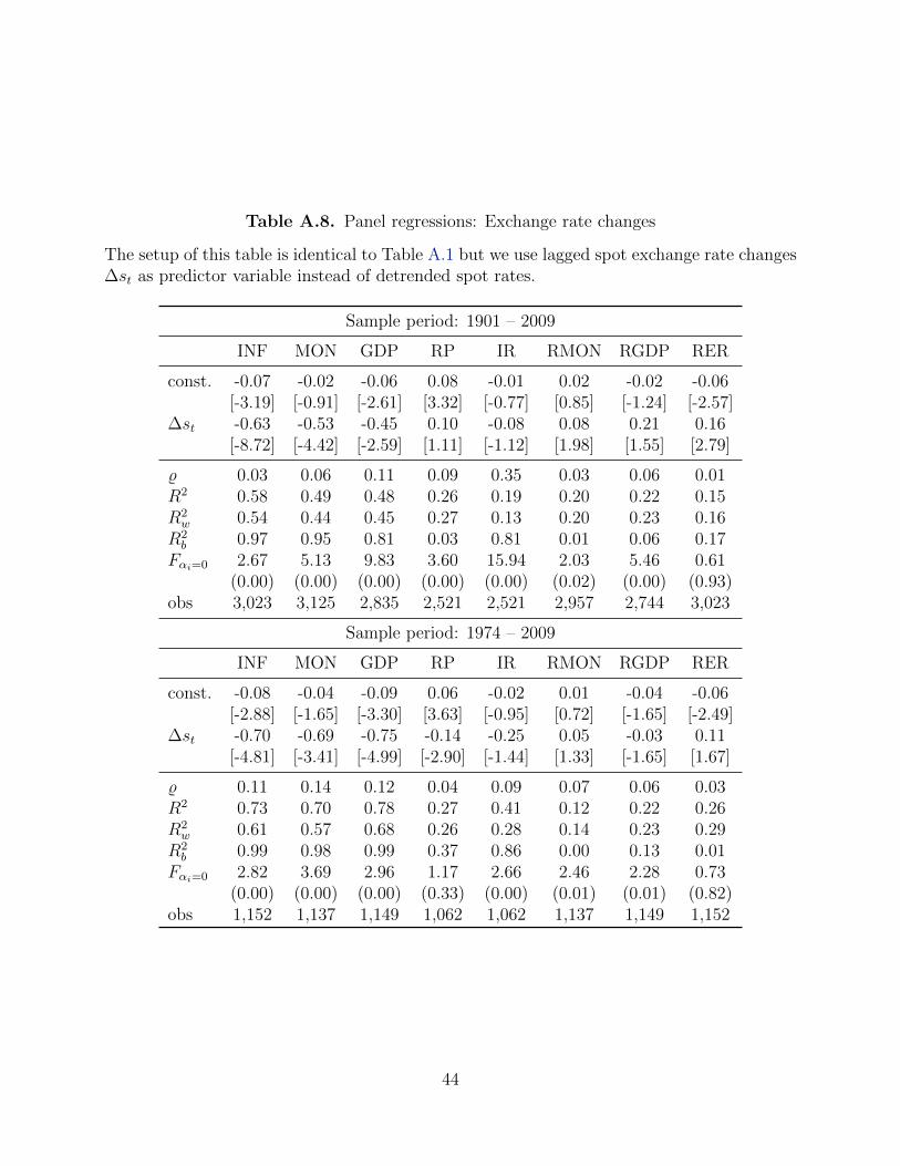
Table A.8. Panel regressions: Exchange rate changes

The setup of this table is identical to Table A.1 but we use lagged spot exchange rate changes∆st as predictor variable instead of detrended spot rates.



const. -0.07 -0.02 -0.06 0.08 -0.01 0.02 -0.02 -0.06[-3.19] [-0.91] [-2.61] [3.32] [-0.77] [0.85] [-1.24] [-2.57]

∆st -0.63 -0.53 -0.45 0.10 -0.08 0.08 0.21 0.16[-8.72] [-4.42] [-2.59] [1.11] [-1.12] [1.98] [1.55] [2.79]

% 0.03 0.06 0.11 0.09 0.35 0.03 0.06 0.01R2 0.58 0.49 0.48 0.26 0.19 0.20 0.22 0.15R2w 0.54 0.44 0.45 0.27 0.13 0.20 0.23 0.16

R2b 0.97 0.95 0.81 0.03 0.81 0.01 0.06 0.17

Fαi=0 2.67 5.13 9.83 3.60 15.94 2.03 5.46 0.61(0.00) (0.00) (0.00) (0.00) (0.00) (0.02) (0.00) (0.93)

obs 3,023 3,125 2,835 2,521 2,521 2,957 2,744 3,023



const. -0.08 -0.04 -0.09 0.06 -0.02 0.01 -0.04 -0.06[-2.88] [-1.65] [-3.30] [3.63] [-0.95] [0.72] [-1.65] [-2.49]

∆st -0.70 -0.69 -0.75 -0.14 -0.25 0.05 -0.03 0.11[-4.81] [-3.41] [-4.99] [-2.90] [-1.44] [1.33] [-1.65] [1.67]

% 0.11 0.14 0.12 0.04 0.09 0.07 0.06 0.03R2 0.73 0.70 0.78 0.27 0.41 0.12 0.22 0.26R2w 0.61 0.57 0.68 0.26 0.28 0.14 0.23 0.29

R2b 0.99 0.98 0.99 0.37 0.86 0.00 0.13 0.01

Fαi=0 2.82 3.69 2.96 1.17 2.66 2.46 2.28 0.73(0.00) (0.00) (0.00) (0.33) (0.00) (0.01) (0.01) (0.82)

obs 1,152 1,137 1,149 1,062 1,062 1,137 1,149 1,152

44

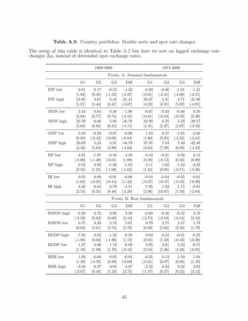
Table A.9. Country portfolios: Double sorts and spot rate changes

The setup of this table is identical to Table A.2 but here we sort on lagged exchange ratechanges ∆st instead of detrended spot exchange rates.

1909-2009 1974-2009



INF low 0.81 0.17 -0.52 -1.33 0.00 -0.56 -1.21 -1.21[1.82] [0.48] [-1.53] [-3.37] [-0.01] [-2.41] [-4.00] [-2.51]

INF high 24.85 4.61 3.44 -21.41 35.67 5.31 3.71 -31.96[5.57] [5.44] [6.47] [-5.07] [4.23] [4.91] [5.02] [-4.01]

MON low 2.44 0.64 0.48 -1.96 -0.67 -0.33 -0.46 0.20[2.88] [0.77] [0.74] [-2.55] [-0.81] [-0.43] [-0.76] [0.30]

MON high 22.59 6.06 5.80 -16.78 34.90 6.25 5.33 -29.57[5.83] [6.85] [6.55] [-4.15] [4.41] [5.37] [3.97] [-3.58]

GDP low 0.83 -0.33 -0.07 -0.90 1.03 0.57 -1.05 -2.08[0.88] [-0.42] [-0.08] [-0.84] [1.60] [0.95] [-2.32] [-2.81]

GDP high 20.69 5.24 3.91 -16.79 37.95 7.83 5.49 -32.46[4.56] [5.83] [4.99] [-4.04] [4.63] [7.29] [6.89] [-4.23]

RP low -4.91 -1.97 -0.58 4.33 0.43 -0.21 0.56 0.13[-2.00] [-1.49] [-0.61] [1.89] [0.28] [-0.12] [0.33] [0.09]

RP high 0.52 0.92 -1.30 -1.82 2.11 1.62 -1.23 -3.33[0.50] [1.25] [-1.08] [-1.62] [1.24] [0.95] [-0.71] [-3.36]

IR low 0.05 0.00 -0.01 -0.06 -0.04 -0.04 -0.05 -0.01[1.05] [-0.05] [-0.14] [-1.22] [-0.37] [-0.47] [-0.43] [-0.09]

IR high 3.30 0.83 0.79 -2.51 7.95 1.33 1.15 -6.81[2.74] [8.35] [8.48] [-2.20] [2.96] [10.87] [7.50] [-2.64]



RMON high -3.20 0.72 0.08 3.28 -2.60 -0.46 -0.42 2.19[-2.59] [0.93] [0.09] [3.10] [-2.73] [-0.58] [-0.54] [2.16]

RMON low 0.75 3.33 2.76 2.01 0.79 2.75 2.57 1.78[0.84] [4.61] [3.74] [2.70] [0.69] [2.60] [2.38] [1.79]

RGDP high -7.50 0.02 -1.22 6.28 0.03 0.52 -0.21 -0.25[-1.88] [0.03] [-1.86] [1.72] [0.05] [1.59] [-0.43] [-0.38]

RGDP low 1.27 0.86 1.19 -0.09 2.95 3.61 2.23 -0.71[1.19] [1.09] [1.78] [-0.10] [3.54] [5.26] [4.23] [-0.85]

RER low 1.69 -0.68 0.85 -0.84 -0.35 0.12 1.59 1.94[1.49] [-0.76] [0.89] [-0.69] [-0.21] [0.07] [0.95] [1.59]

RER high -3.92 0.37 0.94 4.87 -2.32 0.34 0.32 2.64[-2.07] [0.44] [1.23] [2.75] [-1.47] [0.27] [0.22] [3.12]

45

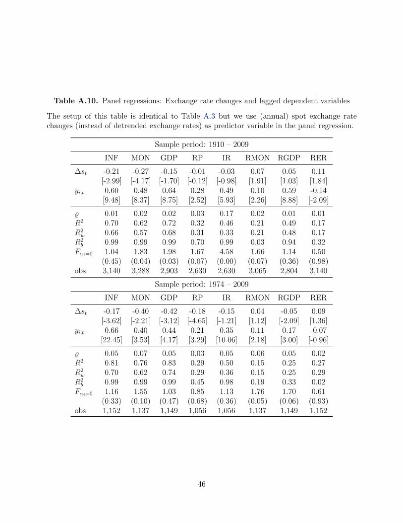
Table A.10. Panel regressions: Exchange rate changes and lagged dependent variables

The setup of this table is identical to Table A.3 but we use (annual) spot exchange ratechanges (instead of detrended exchange rates) as predictor variable in the panel regression.



∆st -0.21 -0.27 -0.15 -0.01 -0.03 0.07 0.05 0.11[-2.99] [-4.17] [-1.70] [-0.12] [-0.98] [1.91] [1.03] [1.84]

yi,t 0.60 0.48 0.64 0.28 0.49 0.10 0.59 -0.14[9.48] [8.37] [8.75] [2.52] [5.93] [2.26] [8.88] [-2.09]

% 0.01 0.02 0.02 0.03 0.17 0.02 0.01 0.01R2 0.70 0.62 0.72 0.32 0.46 0.21 0.49 0.17R2w 0.66 0.57 0.68 0.31 0.33 0.21 0.48 0.17

R2b 0.99 0.99 0.99 0.70 0.99 0.03 0.94 0.32

Fαi=0 1.04 1.83 1.98 1.67 4.58 1.66 1.14 0.50(0.45) (0.04) (0.03) (0.07) (0.00) (0.07) (0.36) (0.98)

obs 3,140 3,288 2,903 2,630 2,630 3,065 2,804 3,140



∆st -0.17 -0.40 -0.42 -0.18 -0.15 0.04 -0.05 0.09[-3.62] [-2.21] [-3.12] [-4.65] [-1.21] [1.12] [-2.09] [1.36]

yi,t 0.66 0.40 0.44 0.21 0.35 0.11 0.17 -0.07[22.45] [3.53] [4.17] [3.29] [10.06] [2.18] [3.00] [-0.96]

% 0.05 0.07 0.05 0.03 0.05 0.06 0.05 0.02R2 0.81 0.76 0.83 0.29 0.50 0.15 0.25 0.27R2w 0.70 0.62 0.74 0.29 0.36 0.15 0.25 0.29

R2b 0.99 0.99 0.99 0.45 0.98 0.19 0.33 0.02

Fαi=0 1.16 1.55 1.03 0.85 1.13 1.76 1.70 0.61(0.33) (0.10) (0.47) (0.68) (0.36) (0.05) (0.06) (0.93)

obs 1,152 1,137 1,149 1,056 1,056 1,137 1,149 1,152

46

Documents

Which Fundamentals Drive Exchange Rates? A Cross … · Which Fundamentals Drive Exchange ... Which Fundamentals Drive Exchange Rates? A Cross-Sectional Perspective ... and investigates