WhichWay

7/27/2019 WhichWay

http://slidepdf.com/reader/full/whichway 1/6

Which Way Did It Go? ‐ The Quantum Eraser

Frank Rioux

Chemistry Department

CSB|SJU

Paul Kwiat and Rachel Hillmer, an undergraduate research assistant, published ʺA Do‐It‐Yourself

Quantum Eraser

ʺ based

on

the

double

‐slit

experiment

in

the

May

2007

issue

of

Scientific

American.

The

purpose of this tutorial is to show the quantum math behind the laser demonstrations illustrated in

this article.

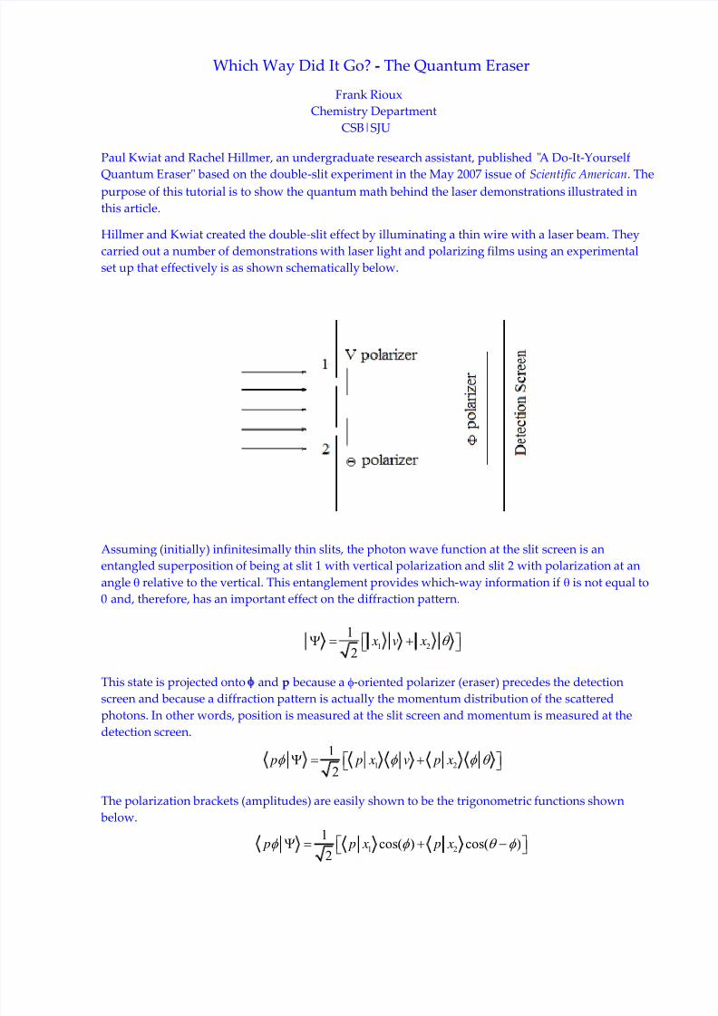
Hillmer and Kwiat created the double‐slit effect by illuminating a thin wire with a laser beam. They

carried out a number of demonstrations with laser light and polarizing films using an experimental

set up that effectively is as shown schematically below.

Assuming (initially) infinitesimally thin slits, the photon wave function at the slit screen is an

entangled superposition of being at slit 1 with vertical polarization and slit 2 with polarization at an

angle relative to the vertical. This entanglement provides which‐way information if is not equal to

0 and, therefore, has an important effect on the diffraction pattern.

1 2

1

2 x v x

This state is projected onto and p because a ‐oriented polarizer (eraser) precedes the detection

screen and because a diffraction pattern is actually the momentum distribution of the scattered

photons. In other words, position is measured at the slit screen and momentum is measured at thedetection screen.

1 2

1

2 p p x v p x

The polarization brackets (amplitudes) are easily shown to be the trigonometric functions shown

below.

1 2

1cos( ) cos( )

2 p p x p x

7/27/2019 WhichWay


The position‐momentum brackets are the position eigenstates in the momentum representation and

are given by,

1exp

2

ipx p x

This allows us to write,

1 21 1 1exp cos( ) exp cos( )

2 2 2

ipx ipx p

Working in atomic units (h = 2) and now assuming slits of finite width this expression becomes,

Slit positions: x1 1 x2 2 Slit width: .2

p x1

2

x1

2

x1

2 exp i p x( )

1

d cos

x2

2

x2

2

x1

2 exp i p x( )

1

d cos

2

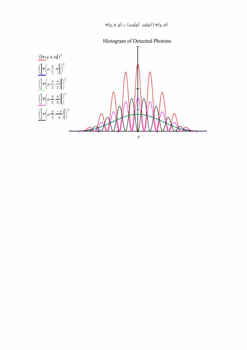
The square of the absolute magnitude of this function yields a representation of the diffraction pattern

as a histogram of photon arrivals on the detection screen. The results shown in the figure will be

discussed below.

Histogram of Detected Photons

p 0 0( ) 2

p

2 0

2

p

2

2

2

p2

4

2

p

2

4

2

p

7/27/2019 WhichWay


Discussion of Results

The polarizer at slit 1 is always oriented vertically so only the orientations ( and ) of the otherpolarizers need to be specified.

[ = 0; = 0] The photons emerging from the slits are vertically polarized and encounter a vertical

polarizer before the detection screen. This is the reference experiment and yields the traditional

diffraction pattern, as shown by the plot of p 0 0( ) 2 . There is no which‐way information in this

experiment and 100% of the photons emerging from the vertically polarized slit screen reach the

detection screen.

p p 0 0( ) 2

d float 3 1.00

[ = /2, = 0] and [ = /2, = /2] The crossed polarizers at the slit screen provide which‐way

information and the interference fringes disappear if the third polarizer is vertically or horizontally

oriented. This is shown by the plots of p 2

0

2

and p 2

2

2

. Furthermore, relative to

the reference experiment, 50% of the photons reach the detection screen.

p p

2 0

2

d float 3 .500

p p

2

2

2

d float 3 .500

In the absence of the third polarizer, there is also no diffraction pattern but 100% of the photons

reach the detection screen.

[ = /2, = /4] and [ = /2, = ‐ /4] The which‐way information provided by the crossed

polarizers at the slit screen is erased by diagonally and anti‐diagonally oriented polarizers in front of

the detection screen. This is shown by the plots of p

2

4

2

and p

2

4

2

. The reason

the which‐way information has been erased is that vertically and horizontally polarized photons

emerging from slits 1 and 2 both have a 50% chance of passing the diagonally or anti‐diagonally

oriented third polarizer. Thus, it is impossible to determine the origin of a photon that passes the third

polarizer and the interference fringes are restored. Again, for this experiment 50% of the photons reach

the detection screen.

p p

2

4

2

d float 3 .500

p p

2

4

2

d float 3 .500

The shift in the interference fringes calculated for p

2

4

2

and p

2

4

2

is observed in

the Kwiat/Hillmer experiment.

7/27/2019 WhichWay


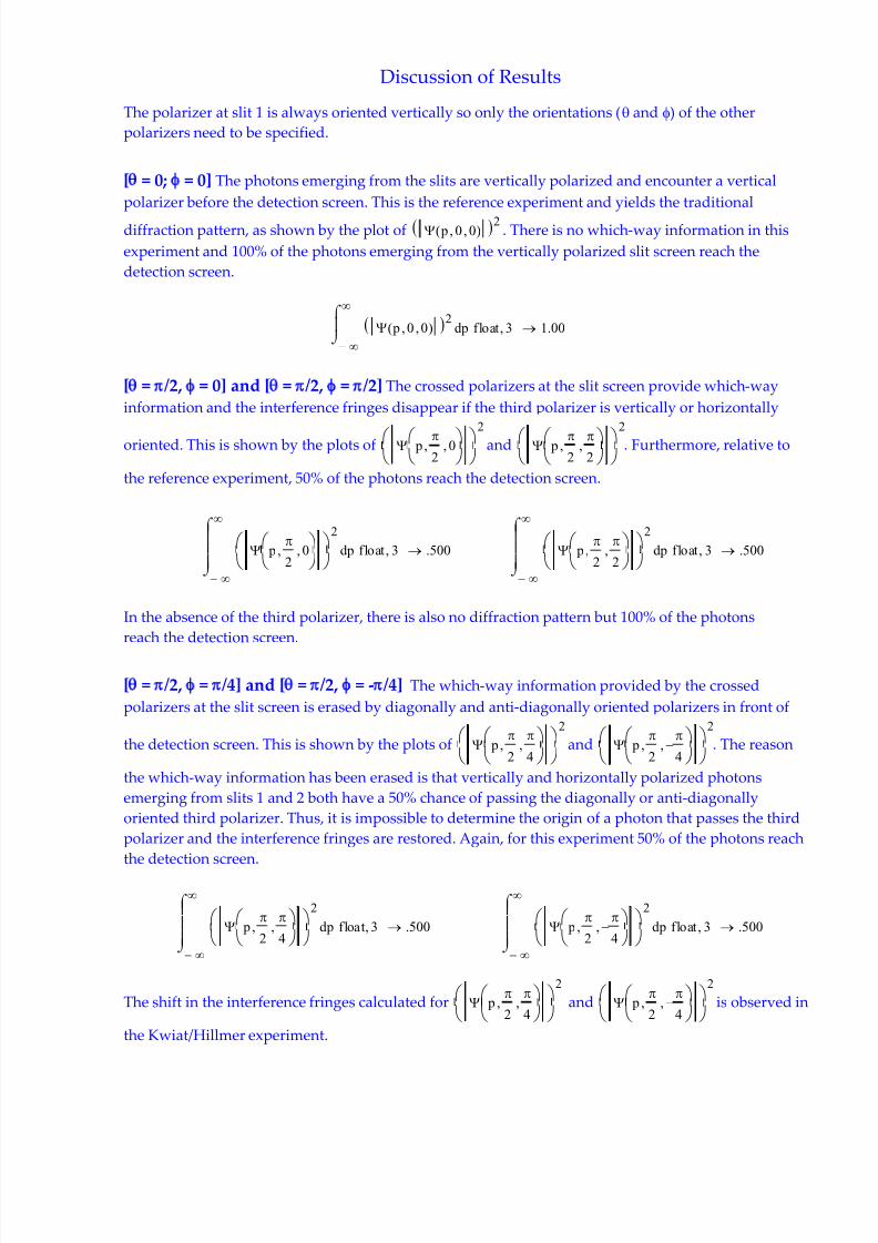
The visibility of the restored fringes is maximized for = +/‐ /4. As the figure belows shows thevisibility is reduced for other values of .


p

2

4

2

p

2

16

2

p

2

8

2

p

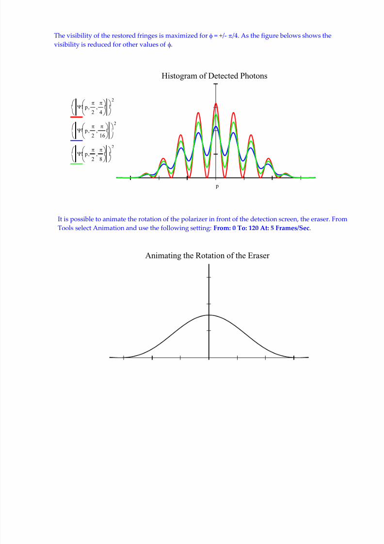
It is possible to animate the rotation of the polarizer in front of the detection screen, the eraser. From

Tools select Animation and use the following setting: From: 0 To: 120 At: 5 Frames/Sec.

Animating the Rotation of the Eraser

7/27/2019 WhichWay


Explicit Vector Approach

In what follows an explicit vector approach to the analysis above is provided.

1 2

1 2 1 2

2

cos( )1 cos( )1 1 1

sin( )0 sin( )2 2 2

p p x p x x v x x x

p x

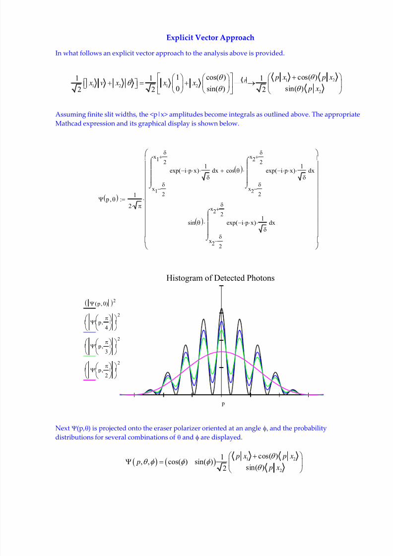
Assuming finite slit widths, the <p|x> amplitudes become integrals as outlined above. The appropriate

Mathcad expression and its graphical display is shown below.

p 1

2

x1

2

x1

2

xexp i p x( )1

d cos

x2

2

x2

2

xexp i p x( )1

d

sin

x2

2

x2

2

xexp i p x( )1

d


p 0( ) 2

p

4

2

p

3

2

p

2

2

p

Next (p,) is projected onto the eraser polarizer oriented at an angle and the probability

distributions for several combinations of and are displayed.

1 2

2

cos( )1, , cos( ) sin( )

sin( )2

p x p x p

p x

7/27/2019 WhichWay


p cos sin p


p 0 0( ) 2

p

2 0

2

p

2

2

2

p

2

4

2

p

2

4

2

p

Documents

WhichWay