Who Benefits from Public Education Provision? Evidence from Italy

Francesco Andreoli (CEPS/INSTEAD, Luxembourg, and University of Verona, Italy)

Giorgia Casalone (University of Verona, Italy)

Daniela Sonedda (University of the Eastern Piedmont Amedeo Avogadro, Italy)

Paper Prepared for the IARIW 33rd

General Conference

Rotterdam, the Netherlands, August 24-30, 2014

Session 6C

Time: Thursday, August 28, Afternoon

Who benefits from public education provision?

Evidence from Italy.∗

Francesco Andreolia,b, Giorgia Casalonec, and Daniela Soneddac,†

aCEPS/INSTEAD 4, avenue de la Fonte, L-4364 Esch sur Alzette, LuxembourgbUniversity of Verona, Via dell’Artigliere 19, I-37129 Verona, Italy.

cUniversity of the Eastern Piedmont Amedeo Avogadro, via Perrone 18, I-28100 Novara, Italy.

July 2014

Abstract

Public education provision is redistributive when rich families, who contribute to itsfinancing, find it optimal to sort out of the public system and buy the educationalservices on the private market. This may occur if the quality of the educationalservices is lower in the public sector than it is in the private. We estimate structuralquantile treatment effects to analyze the mechanisms behind the redistributiveness ofpublic education provision using Italian data. We exploit heterogeneity in expectedtax deductions to exogenously manipulate the distribution of net of taxes income,equalized by families needs, and explore the consequences of this manipulation onvarious quantiles of the distribution of the amount of the educational transfers inkind. We find that an increase in income reduces the amount of educational transfersin-kind (i) more for higher quantiles of the educational transfers in-kind (ii) more forlower quantiles of the households’ earning capacity. Our findings explain how, forcompulsory schooling, the households’ sorting into private education may motivate agovernment, that aims at redistributing resources from the rich to the poor, to usepublic education provision as transfers in-kind.

Keywords: Transfer in kind, public education provision, income distribution, structural

quantile treatment effects.

JEL Codes: H40, D30, I20.

∗We are grateful to Rolf Aaberge, Erich Battistin, Lorenzo Cappellari, Daniele Checchi, Carlo Fio-

rio, Paolo Ghinetti, Arnaud Lefranc, Enrico Rettore, Francesca Zantomio and Claudio Zoli for valuable

comments. We thank participants at conferences and seminars held at Aix-en-Provence (LAGV), Bari

(ECINEQ), Canazei, IRVAPP, Novara, Pavia and Torino for useful comments. We also thank Carlo Fiorio

for kindly providing us data on gross income and personal income taxes. We are fully responsible for any

errors.†Corresponding author.

Contacts: francescondrl@gmail.com (F. Andreoli), giorgia.casalone@eco.unipmn.it (G. Casalone) and

daniela.sonedda@eco.unipmn.it (D. Sonedda).

1

1 Introduction

In Italy, as in many other countries, public education provision and free accessibility to

compulsory education are fundamental constitutional rights. Determining the optimal

amount of resources devoted to finance educational services is a relevant economic issue.

As largely recognized, public education provision, together with health care, account for a

substantial share of the public budget in countries with developed welfare states. Several

reasons justify this spending: among them, a redistributive motive (see Aaberge, Langor-

gen and Lindgren 2013).

This paper aims at analyzing the mechanisms behind the redistributiveness of public

education provision using Italian data. Public education provision is redistributive as far

as more affluent families, who contribute to its financing, find it optimal to sort out of the

public system, and buy the educational services on the private market. Different reasons

may justify why families choose private schools. We will focus on the interplay between

the family resources and school quality, although other factors such as the support of

common values (e.g., religion (Sander 2001) and status symbol (Fershtman, Murphy and

Weiss 1996)) also play a relevant role.

There is a long tradition within the human capital investment models (see for instance

Stiglitz 1974) of claiming that the quality embedded in private schools is higher than in

public schools. If this is the case, since quality is a normal good, rich households prefer

an higher amount of this quality level, and they may opt out for private education even if

having to pay for it. Quality can be conceived either as a subjective measure of schools’

quality, such as the score given by households to the schools in the area of residence, or a

more objective measure, linked to observable indicators such as the student-teacher ratio

(Checchi and Jappelli 2003).

The choice of producing a lower quality level in the public sector is at the heart of

the redistributive nature of educational transfers in-kind. This paper focuses on a specific

mechanism operating through the quality of the education system, according to which the

different sorting of the families into private schooling may motivate a government, that

aims at redistributing resources from the rich to the poor, to use public education provision

as transfers in-kind. The literature that analyses the role of public education provision

(educational transfers in-kind) calls this sorting process into private and public education

self-targeting (Currie and Gahvari 2008).

The policymaker with redistributive intents imposes costs that may take the form of

restrictions on the quality of the public educational service, or on the heterogeneity and

personalization of the curricula. Such costs deter the rich households from mimicking

the poor ones, thus acting as a separation device. The lower is the quality, the larger

is the incentive of the households with higher earning capacity to sort out of the public

2

education system while continuing to finance it, which makes the educational transfers

in-kind progressive in nature (Besley and Coate 1991, Blackorby and Donaldson 1988).

The quality of public education should be, however, high enough to insure an adequate

service to low income families, who would otherwise bear only the cost associated to this

mechanism. This reasoning applies in full only to mandatory education, where families can

decide whether to enroll their children in the public or in the private sector, but they have

no option left for choosing to consume no educational service. Whether the mechanism

also works in post-mandatory education (i.e. for families with kids aged more than 14 years

old) is debatable for at least two reasons. First, the household’s self-selection into both

private and public education can be driven by expected returns to kid’s education that are

positively correlated with family income. Second, the quality of private schooling for upper

secondary education is not necessarily higher than that related to public schools. This

occurs, for instance, in Italy as a consequence of the demand for private education of less

talented kids coming from rich households (Bertola, Checchi and Oppedisano 2007, Bertola

and Checchi 2013).

This paper proposes to convert the quality of the public education provision, inter-

preted as educational transfers in-kind, into a monetary counterpart that the family would

have to spend to buy the same quality on the market. This quantity is the monetary

equivalent of a transfer in-kind that the family receives when opting for inexpensive public

education. It represents a lower bound of the opportunity costs to choose private educa-

tion. Following the standard practice, we assume that the value of the educational transfer

in-kind received by each student is equal to the average cost of producing the services this

student benefit from. Since one of the main component of this average cost of producing

the public education services is the teacher-student ratio, our measure of the educational

transfers in-kind reflects the objective quality of the public service.

One of the major difficulties in this type of analysis is related to data availability.

Aaberge, Bhuller, Langørgen and Mogstad (2010), for instance, use detailed accounting

data of municipalities as a basis for estimating the need adjusted scale for local public ser-

vices in Norway. We make use of a study carried out exclusively for year 2003 by the Italian

National Institute for the Evaluation of Education System (INVALSI) and the Consortium

for the Development of the Methodologies and Innovations of the Public Administrations

(MIPA), INVALSI-MIPA (2005), to microsimulate the educational transfers in-kind ac-

cruing to the households. We use SHIW database (wave 2004) by the Bank of Italy to

collect the other data of interest, such as household income, children school attendance

and information on the background of origin of the family. Since SHIW does not provide

information on the type of school (public versus private) attended by children, we weight

the per-child educational transfer in-kind by group-specific probabilities to be enrolled in

3

a public school/university.

This paper contributes to the limited empirical evidence on the relationship between

family income and educational transfers in-kind redistributiveness, by analyzing the premises

of the mechanism driving the sorting process into public and private education among

Italian households. At the heart of the sorting process into private education, there is the

correlation between the unobservable family specific earning capacity and preference for

quality of the education good. It is precisely their correlation that affects the incidence of

the self-targeting mechanisms. To assign our results with a causal interpretation, we need

to single out the exogenous effect of income. We exploit heterogeneity in expected tax

deductions to exogenously manipulate the prevailing distribution of net of taxes income,

equalized by families needs, and explore the consequences of this manipulation on various

quantiles of the distribution of the amount of educational transfers in-kind.

On the one hand, for a given degree of quality, proxied by the quantiles of the distribu-

tion of the educational transfers in-kind, the household’s earning capacity determines the

access into private education. We expect therefore that an increase in household income is

associated with decreasing transfers in-kind that goes to the household with higher earning

capacity. On the other hand, for a given degree of the household’s earning capacity, prox-

ied by the quantiles of the distribution of household earning capacity, the quality of public

schools as measured by our transfers in-kind, may explain the sorting into private and

public education. In this case, the magnitude of the negative relation between household

income and the transfers in-kind she receives is expected to grow along the distribution

of in-kind transfers, since households revealing higher preferences for the quality of educa-

tional services will be ready to devote a large share of a marginal income gain into private

education.

Our analysis shows that an increase in income reduces the amount of educational

transfers in-kind (i) more for higher quantiles of the educational transfers in-kind (ii) more

for lower quantiles of the household earning capacity. These results are strengthened when

we confine our analysis to compulsory education only.

The rest of the paper is organized as follows. Section 2 sets the scene illustrating how

and when public education provision is redistributive and describing the microsimulation

exercise on the educational transfers in-kind. Section 3 describes the data, our instrument,

and the method. Results and the discussion are reported in section 4. Finally, section 5

concludes.

4

2 Public education provision and in-kind transfers

2.1 Quality sorting and educational transfers in-kind

We illustrate through graphic analysis the mechanism connecting sorting on quality, house-

hold earning capacity, and private or public educational choices according to the model by

Besley and Coate (1991), as presented by Gahvari and Mattos (2007). Assume that two

goods are produced within the economy: a numeraire consumption good c and a publicly

provided indivisible (education) good. Producers are assumed to behave competitively and

p defines the price of quality at the margin under linear technology. There are two types

of households: the poor households with low income yP and the rich households with high

income yR, such that yP < yR. The publicly-provided educational services are financed

by a personal tax T .

Households may choose to consume only one of the two variants of the education good

produced in the sector while caring about its quality k (i.e. families may consume either

private or public sector education) which is a normal good. The production of each variant

of the educational services embodies a specific quality level. This implies that households

with higher income levels may prefer to opt out for higher quality variants of the good even

if this means having to support in full its cost in the private sector. To get redistribution

through public education provision, however, the policymaker needs to implement a second

or even third best allocation of resources.

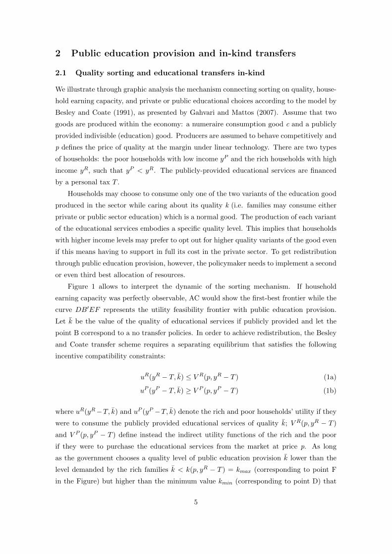
Figure 1 allows to interpret the dynamic of the sorting mechanism. If household

earning capacity was perfectly observable, AC would show the first-best frontier while the

curve DB′EF represents the utility feasibility frontier with public education provision.

Let k̄ be the value of the quality of educational services if publicly provided and let the

point B correspond to a no transfer policies. In order to achieve redistribution, the Besley

and Coate transfer scheme requires a separating equilibrium that satisfies the following

incentive compatibility constraints:

uR(yR − T, k̄) ≤ V R(p, yR − T ) (1a)

uP (yP − T, k̄) ≥ V P (p, yP − T ) (1b)

where uR(yR−T, k̄) and uP (yP −T, k̄) denote the rich and poor households’ utility if they

were to consume the publicly provided educational services of quality k̄; V R(p, yR − T )

and V P (p, yP − T ) define instead the indirect utility functions of the rich and the poor

if they were to purchase the educational services from the market at price p. As long

as the government chooses a quality level of public education provision k̄ lower than the

level demanded by the rich families k̄ < k(p, yR − T ) = kmax (corresponding to point F

in the Figure) but higher than the minimum value kmin (corresponding to point D) that

5

Figure 1: The Economy’s Pareto Frontier (AC) and Utility Feasibility Frontier (DB′EF )with public education provision when kmax > k∗.

satisfies equation (1b), rich and poor families self-target with respect to participation to

the program.

The same figure illustrates the deadweight loss associated to the program. Only point

E is on the first best frontier corresponding to the efficient quality level k∗ that makes the

poor households indifferent between receiving one extra euro in cash and one extra euro

worth of the publicly provided educational services such thatU ′k̄=k∗U ′c

= p.1 For all points

between D and E, the quality level chosen by the government is less than efficient, k̄ ≤ k∗,while for all points between E and F the quality level is more than efficient k̄ ≥ k∗. To

account for these inefficiencies, Gahvari and Mattos (2007) show that a combination of

cash (in terms of either a cash rebate or a lump sum tax) and in-kind transfers may allow

to achieve first-best redistribution with self-targeting mechanisms.

The incentive compatibility constraint of the rich in equation (1a) sets the limit on the

redistributiveness of the program and for this reason, such schemes may not necessarily

form part of a properly designed redistributional packages. Although there is self-selection

in taking up the program on the side of the poor households, the efficient quality of the

public provision of education that the poor families would choose for themselves if they

1Figure 1 illustrates the case where kmax ≥ k∗, when kmax ≤ k∗ the utility feasibility frontier iseverywhere inside the Pareto frontier.

6

receive its value in cash, remains unobservable. This implies a trade-off between the cost

to the government to minimize the asymmetric information on the households’ earning

capacity and the deadweight loss inherent in an inefficient quality of the public provision

of education.

2.2 Public educational services as transfers in-kind

The evaluation of educational transfers in-kind is an empirical demanding exercise whose

difficulty motivates the little evidence about the behavior of the households in the sorting

process into either private or public education.

One of the reason for this limitedness is data availability for educational transfers

in-kind. We make use of a unique study by (INVALSI-MIPA 2005) based on year 2003

data to compute the educational transfers in-kind monetary equivalent. The value of

the educational transfers in-kind received by each student is equal to the average costs

of producing it, denoted AC(r, e), which is allowed to vary across Italian regions r and

educational levels e.2 This monetary value summarizes the information provided by a

variety of indicators representing the quality of the schooling inputs. The most relevant of

these indicators is the teacher-pupils ratio, a well known measure of educational quality.

We merge these average costs with data collected by the Bank of Italy, SHIW (Survey

on Households Income and Wealth) 2004 wave. We treat as recipients of the transfers

all children in a family, aged between 3 and 5 years, and those aged from 6 to 23 years

who classify themselves as students in the survey. Unfortunately, we do not observe the

type (i.e. either private or public) of school attended by the students. Consequently, we

assign to each student the cost of production of the education service he is consuming

in his region of residence and for his educational level, discounted by the probability he

has to benefit of public education. Denote this probability by ω(g), which is specific to a

set g of household characteristics. It encapsulates the information on the school selection

process from the side of the households. The monetary value of the educational transfer

in-kind associated to each child c in family h of type gh, who lives in region rc and who is

in educational level ec is denoted:

kc := ω(gh) ·AC(rc, ec) for c ∈ h. (2)

To compute ω(gh) we use ISTAT, Multiscopo Survey data for year 2005, the closest

to year 2004, that provides information on whether the interviewed family has a child

2Since Italy has 20 regions and 5 educational levels (from kindergarten to tertiary education), we endup with a 20×5 matrix of average costs of education. For all details about the calculations of these averagecosts see appendix A.

7

enrolled either in a private or in a public school.3 We collapse those families with children

in education into homogenous groups denoted by g according to a variety of household

characteristics, such as the macro geographical area of residence, age class of each child,

level of education of the parents and occupational conditions of the head of the family.4

For each group g, we use observed frequencies to determine the probabilities to enroll a

children in public education. We then use these group specific probabilities ωg to calculate

the expected value of the educational transfer in-kind for each children. Two children in

education who live in the same region, attend the same educational level and come from

families in the same class, receive equal (expected) value of educational transfers in-kind.

The resulting distribution of in-kind transfers accruing to each child is heterogeneous across

groups of families, regions and educational levels.5

The transfer in-kind accruing to the household h corresponds to the sum of the transfers

received by each of her children in education, and it is denoted:

kh =∑c∈h

kc. (3)

The first source of heterogeneity in the distribution of kh is related to the differences,

across groups of households, in the preferences for quality of the educational services, which

determines the choice of private versus public provision and to the variation in the public

education priorities across educational levels of regional governments. The second source

of heterogeneity is instead related to the tastes for education reflected in the number of

children attending schools. The latter source plays a role only for kids in post-compulsory

education.

To make comparable families with different educational needs, we scale kh by the needs-

adjusted equivalence scale (see Aaberge et al. 2013, Aaberge et al. 2010).6 Nevertheless,

3Unfortunately Multiscopo Survey data do not gather information on households’ income.4Geographical areas are North West, North East, Centre and South and Islands. Age classes correspond

to the five educational levels: kindergarten (i.e. from 3 to 5), primary education (i.e. from 6 to 10), lowersecondary education (i.e. from 11 to 13), upper secondary education (i.e. from 14 to 18), and tertiaryeducation (from 19 to 23). Parents’ education is categorized in three levels: low educational level (bothparents with at most lower secondary school degree), high educational level (both parents with uppersecondary school or university degree) and mixed residual category (one parent with a low educationallevel while the other with a high educational level). We consider the lower secondary school degree as thecut-off point since the parents are almost all affected by the 1962 reform which abolished the second trackof the schooling system and made compulsory to all children the attendance of the lower secondary schoolat least up to the age of 14. Finally we identify two different occupational conditions of the households’head: the one (the low-background group) includes unemployed, unskilled manual workers and employeesin the agriculture sector, the other (the high-background group) comprises all other cases.

5For instance, within a region, the expected educational transfers in-kind may take 30 different positivevalues, 5 educational level times 6 different probabilities of attending public schools and a zero value forthose in post-compulsory schooling age who choose stop studying.

6The Simplified Needs-Adjusted equivalence scale (SNA) calculated by Aaberge et al. (2013) for year2006, the closest to year 2004, amounts to assign to all household components other than kids a weight of0.5, and to each kid different weights according to her age: from 3 to 5 years old, 0.3; from 6 to 13, 0.66;from 14 to 23, 0.93.

8

the amount of educational transfers in-kind is per equivalent kid enrolled at schools since

the equivalence scale neutralize for the households’ size and composition conditional on

the kid enrollment at school. All children in post-compulsory schooling age that do not

attend any school take the value of educational transfers in-kind equal to zero.

2.3 Implications of the sorting mechanism

The household’s sorting mechanism into private education may justify the existence of

public education provision as a redistributive transfers program. Its premises can be for-

mulated as hypothetical effects of household income on the in-kind transfer distribution.

This paper uses an identification strategy that allows to estimate the marginal effect (i.e.

the marginal benefit) of income on the amount of educational transfers in-kind chosen by

the families across two relevant distributional dimensions.

For a given degree of quality, proxied by a finite quantile of the distribution of the edu-

cational transfers in-kind, household’s earning capacity can be one of the main determinant

of the access into private education. The model by Besley and Coate (1991) clarifies the

concepts showing that when the households’ earning capacity is unobservable, restrictions

on the quality of the public educational service may deter rich households from mimicking

the poor ones. Together with household earning capacity, quality is, therefore, the other

relevant dimension.

For a degree of the household’s earning capacity, proxied by a finite quantile of the

distribution of the household earning capacity, the quality of public schools as measured

by our transfers in-kind, may explain the type of school chosen. As long as households

give up the quality of public schools freely provided they are revealing a preference for the

quality of private schools.

Our empirical exercise measures the extent to which households income influences

the benefit received by the public education provision across families, characterized by

different earning capacities and different preferences for the quality of the educational

services. Public education provision is redistributive if families sort themselves into private

education as the government expect them to. This occurs if households that benefit less

from public education are those families, for a given quality level, who have an higher

earning capacity, and who have higher preferences for quality, for a given earning capacity.

The empirical analysis detailed below follows these arguments in order to assess whether

redistributionally motivated public education provision is justified.

9

3 Empirical strategy

3.1 SHIW Data: sample selection criteria

We make use of the SHIW (Survey on Households Income and Wealth) 2004 wave. SHIW

is a nationally representative household survey conducted in Italy every two years by the

Bank of Italy and gathers information on net incomes, savings and main characteristics of

Italian households.7 Individual data are collapsed into family income, providing a sample

of 8,012 families of which eight of them are dropped since their income was either negative

or zero.

The sample selection process is based on two data cuts. The Italian educational system

has three main levels which start at the age of six. Before compulsory schooling, from the

age of three, children attend the kindergarten which is generally publicly financed either by

the State or by the local communities. Since families with children at kindergarten benefit

from public education expenditures we include them in the main analysis. Consequently,

we restrict our main sample to families that are potentially entitled to benefit from public

spending on education, namely families with school-age children aged from 3 to 23 years

old.8 This amounts to run our estimates on families with children born between 1981 and

2001. The sample is then reduced to 2,495 households, 271 of which are dropped because

of missing information on either the grandparental background, that we use as covariate

to account for household unobserved heterogeneity, or on the education level of the head

of the family that we use as covariate.9

The social structure of an economy changes over time generating potentially, for a

given survey wave, a composition effect related to different age composition of the family

heads coming from different grandparental backgrounds and living different moments of

the life cycle. To prevent this composition effect we cut the lower and the upper 5% of

the distribution of the age of the head of the family restricting our sample to families

whose head aged from 33 to 60 years old at the time of the survey (i.e. individuals born

between 1944 and 1971) ending up with 2,030 observations for whom descriptive statistics

is reported in Table 1.

To account for scale economies within the household, we equalize household income

using the EU equivalence scale which we consider to be the more appropriate scale since

7Microsimulated gross income data and personal income taxes are kindly provided by C. Fiorio. Thesedata account for potential tax evasion. For this reason, they constitute a more precise measure of theincome earned by the family.

8In Italy a university degree is obtained conditional on passing a certain number of exams. This numbervaries across courses degree. To avoid selection into achievement, we exclude from our working samplefamilies with children aged more than 23. This age can be conceived, in the majority of cases, the minimumage required to complete a university course degree.

9Sixteen of these drops only were due to missing information on the level of education of the head ofthe family.

10

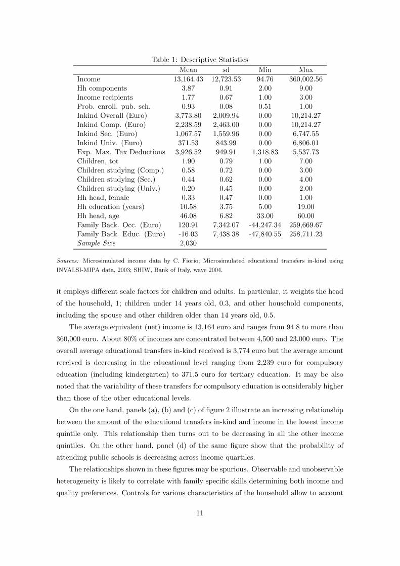
Table 1: Descriptive Statistics

Mean sd Min Max

Income 13,164.43 12,723.53 94.76 360,002.56Hh components 3.87 0.91 2.00 9.00Income recipients 1.77 0.67 1.00 3.00Prob. enroll. pub. sch. 0.93 0.08 0.51 1.00Inkind Overall (Euro) 3,773.80 2,009.94 0.00 10,214.27Inkind Comp. (Euro) 2,238.59 2,463.00 0.00 10,214.27Inkind Sec. (Euro) 1,067.57 1,559.96 0.00 6,747.55Inkind Univ. (Euro) 371.53 843.99 0.00 6,806.01Exp. Max. Tax Deductions 3,926.52 949.91 1,318.83 5,537.73Children, tot 1.90 0.79 1.00 7.00Children studying (Comp.) 0.58 0.72 0.00 3.00Children studying (Sec.) 0.44 0.62 0.00 4.00Children studying (Univ.) 0.20 0.45 0.00 2.00Hh head, female 0.33 0.47 0.00 1.00Hh education (years) 10.58 3.75 5.00 19.00Hh head, age 46.08 6.82 33.00 60.00Family Back. Occ. (Euro) 120.91 7,342.07 -44,247.34 259,669.67Family Back. Educ. (Euro) -16.03 7,438.38 -47,840.55 258,711.23Sample Size 2,030

Sources: Microsimulated income data by C. Fiorio; Microsimulated educational transfers in-kind using

INVALSI-MIPA data, 2003; SHIW, Bank of Italy, wave 2004.

it employs different scale factors for children and adults. In particular, it weights the head

of the household, 1; children under 14 years old, 0.3, and other household components,

including the spouse and other children older than 14 years old, 0.5.

The average equivalent (net) income is 13,164 euro and ranges from 94.8 to more than

360,000 euro. About 80% of incomes are concentrated between 4,500 and 23,000 euro. The

overall average educational transfers in-kind received is 3,774 euro but the average amount

received is decreasing in the educational level ranging from 2,239 euro for compulsory

education (including kindergarten) to 371.5 euro for tertiary education. It may be also

noted that the variability of these transfers for compulsory education is considerably higher

than those of the other educational levels.

On the one hand, panels (a), (b) and (c) of figure 2 illustrate an increasing relationship

between the amount of the educational transfers in-kind and income in the lowest income

quintile only. This relationship then turns out to be decreasing in all the other income

quintiles. On the other hand, panel (d) of the same figure show that the probability of

attending public schools is decreasing across income quartiles.

The relationships shown in these figures may be spurious. Observable and unobservable

heterogeneity is likely to correlate with family specific skills determining both income and

quality preferences. Controls for various characteristics of the household allow to account

11

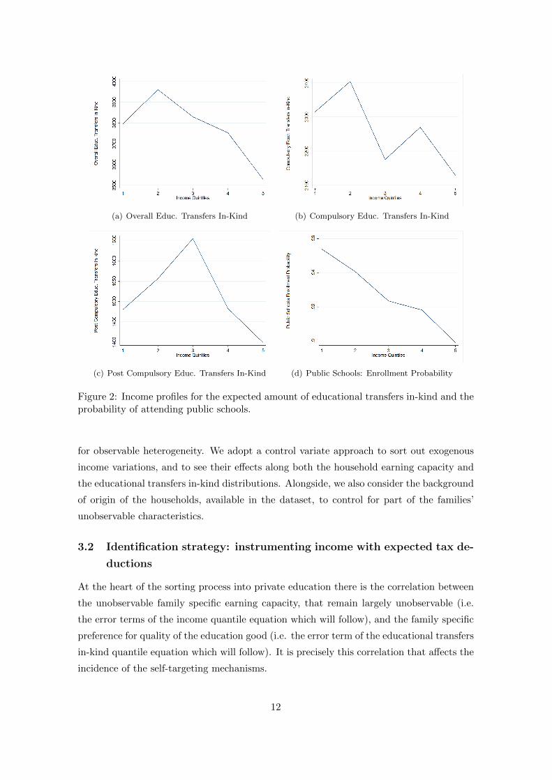
(a) Overall Educ. Transfers In-Kind (b) Compulsory Educ. Transfers In-Kind

(c) Post Compulsory Educ. Transfers In-Kind (d) Public Schools: Enrollment Probability

Figure 2: Income profiles for the expected amount of educational transfers in-kind and theprobability of attending public schools.

for observable heterogeneity. We adopt a control variate approach to sort out exogenous

income variations, and to see their effects along both the household earning capacity and

the educational transfers in-kind distributions. Alongside, we also consider the background

of origin of the households, available in the dataset, to control for part of the families’

unobservable characteristics.

3.2 Identification strategy: instrumenting income with expected tax de-

ductions

At the heart of the sorting process into private education there is the correlation between

the unobservable family specific earning capacity, that remain largely unobservable (i.e.

the error terms of the income quantile equation which will follow), and the family specific

preference for quality of the education good (i.e. the error term of the educational transfers

in-kind quantile equation which will follow). It is precisely this correlation that affects the

incidence of the self-targeting mechanisms.

12

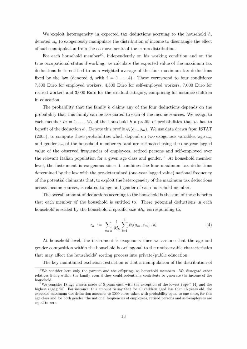
We exploit heterogeneity in expected tax deductions accruing to the household h,

denoted zh, to exogenously manipulate the distribution of income to disentangle the effect

of such manipulation from the co-movements of the errors distribution.

For each household member10, independently on his working condition and on the

true occupational status if working, we calculate the expected value of the maximum tax

deductions he is entitled to as a weighted average of the four maximum tax deductions

fixed by the law (denoted di with i = 1, . . . , 4). These correspond to four conditions:

7,500 Euro for employed workers, 4,500 Euro for self-employed workers, 7,000 Euro for

retired workers and 3,000 Euro for the residual category, comprising for instance children

in education.

The probability that the family h claims any of the four deductions depends on the

probability that this family can be associated to each of the income sources. We assign to

each member m = 1, . . . ,Mh of the household h a profile of probabilities that m has to

benefit of the deduction di. Denote this profile ψi(am, sm). We use data drawn from ISTAT

(2003), to compute these probabilities which depend on two exogenous variables, age am

and gender sm of the household member m, and are estimated using the one-year lagged

value of the observed frequencies of employees, retired persons and self-employed over

the relevant Italian population for a given age class and gender.11 At household member

level, the instrument is exogenous since it combines the four maximum tax deductions

determined by the law with the pre-determined (one-year lagged value) national frequency

of the potential claimants that, to exploit the heterogeneity of the maximum tax deductions

across income sources, is related to age and gender of each household member.

The overall amount of deductions accruing to the household is the sum of these benefits

that each member of the household is entitled to. These potential deductions in each

household is scaled by the household h specific size Mh, corresponding to:

zh :=∑m∈h

1

Mh

4∑i=1

ψi(am, sm) · di (4)

At household level, the instrument is exogenous since we assume that the age and

gender composition within the household is orthogonal to the unobservable characteristics

that may affect the households’ sorting process into private/public education.

The key maintained exclusion restriction is that a manipulation of the distribution of

10We consider here only the parents and the offsprings as household members. We disregard otherrelatives living within the family even if they could potentially contribute to generate the income of thehousehold.

11We consider 18 age classes made of 5 years each with the exception of the lowest (age≤ 14) and thehighest (age≥ 95). For instance, this amount to say that for all children aged less than 15 years old, theexpected maximum tax deduction amounts to 3000 euros taken with probability equal to one since, for thisage class and for both gender, the national frequencies of employees, retired persons and self-employees areequal to zero.

13

(a) Conditional Mean Exp. given Educ. Levels (b) Scatter Educ. In-kind on Exp. Tax Ded.

Figure 3: Validating the Exclusion Restriction.Note: Educational levels are calculated as follows: the value of zero corresponds to any educational level

attended (households with children in post-compulsory schooling age that stopped studying); the values

of 1, 2, and 3 correspond to all household with at least one child in compulsory (1), upper secondary (2)

and tertiary education (3). Household with more than one child are categorized as 3.2 if having at least

one child in compulsory and one in secondary education; 3.4 if having at least one child in compulsory and

tertiary education; 3.6 if having at least one child in secondary and tertiary education and finally 3.8 if

having at least one child in all educational level.

the expected tax deductions Z affects the quantiles of the distribution of the educational

transfers in kind K only because it acts on the prevailing household’s income distribution

Y . This amounts to saying that the household structure, the age and gender composition

within the household have no direct effect on the amount of educational transfers in-kind

from which the household benefit.

The instrumental variable zh might be correlated with children age, thus rising poten-

tial concerns about the validity of the exclusion restriction. The expected tax deductions

do not have, however, an impact on the transfers in-kind received by the household when

conditioned for the age profiles of the children. In fact, if the children is in compulsory

schooling age, then he receives a fixed amount of benefits of 3,000 Euros while the amount

of educational transfers in-kind is always positive and heterogeneous according to the ed-

ucational level (either primary or lower secondary), the region and the reference group of

the family to which the household belongs. Also for children in post-compulsory schooling

age the IV has not a direct effect on the transfer in-kind, because it is independent of the

true working condition of the child while the amount of the educational transfers in-kind

depends upon his educational status.

Figure 3 provides graphical evidence on the validity of the exclusion restriction. Ex-

pected tax deductions are quite flat across educational levels but slightly increasing for

households with children older than 14 years old since the national frequencies of em-

ployees and self-employees is positive for them. At any rate, even if there might exist a

14

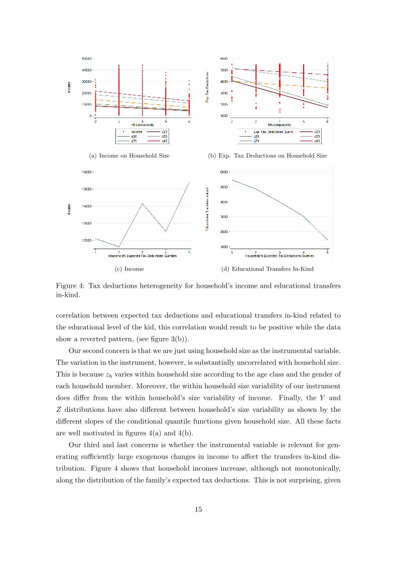
(a) Income on Household Size (b) Exp. Tax Deductions on Household Size

(c) Income (d) Educational Transfers In-Kind

Figure 4: Tax deductions heterogeneity for household’s income and educational transfersin-kind.

correlation between expected tax deductions and educational transfers in-kind related to

the educational level of the kid, this correlation would result to be positive while the data

show a reverted pattern, (see figure 3(b)).

Our second concern is that we are just using household size as the instrumental variable.

The variation in the instrument, however, is substantially uncorrelated with household size.

This is because zh varies within household size according to the age class and the gender of

each household member. Moreover, the within household size variability of our instrument

does differ from the within household’s size variability of income. Finally, the Y and

Z distributions have also different between household’s size variability as shown by the

different slopes of the conditional quantile functions given household size. All these facts

are well motivated in figures 4(a) and 4(b).

Our third and last concerns is whether the instrumental variable is relevant for gen-

erating sufficiently large exogenous changes in income to affect the transfers in-kind dis-

tribution. Figure 4 shows that household incomes increase, although not monotonically,

along the distribution of the family’s expected tax deductions. This is not surprising, given

15

the regressive nature of income tax deductions in presence of increasing marginal personal

income tax rates. In such a case, higher (net) income quintiles benefit more from tax

deductions. The amount of educational transfers in-kind is lower for higher quintiles of

the expected tax deductions (figure 4(d)). These two graphs hint that the reduced form

regression of an exogenous manipulation of the prevailing distribution of incomes on vari-

ous quantiles of educational transfers in-kind distribution would estimate a negative effect

of the former on the latter variable.

3.3 Structural quantile treatment effect estimation method

Making use of a particular feature of the 1993 SHIW wave, Checchi and Jappelli (2007)

estimate the conditional mean probability of enrollment in private schools controlling for

income quartile, both a subjective and an objective quality indicators and other covari-

ates. Their empirical evidence suggests that rich households are more likely to use private

education while the perceived quality of public schools measured by a self-reported qual-

ity score is negatively correlated with the probability of attending private schools. The

selection mechanism presented in section 2.1 suggests that public education provision is

redistributive if households that benefit less from public education are those with higher

earning capacity, for a given degree of quality level, and those who have higher preferences

for quality, for a given degree of earning capacity.12

We apply the control variate approach by Ma and Koenker (2006) to exogenously ma-

nipulate the income distribution and to estimate the structural quantile treatment effects

of exogenous variations of income on the distribution of transfer in-kind received by the

families. This method is the most appropriate to measure the extent to which households

income influences the benefit received by the public education provision heterogeneously

across families earning capacity and preferences for the quality of the educational services.

This double heterogeneity in the income effects allows to assess the implications of the

sorting mechanisms on the distribution of transfers in-kind across families with children in

education.

Consider the following quantile functions of the response variables transfers in-kind,

denoted QK , and household income, denoted QY . In what follows, we use capital letters to

indicate distributions, while bold letters refer to either vectors or matrices. The analysis

is at the household level and the subscript h is dropped for expositional purposes. We

12According to the Besley and Coate (1991) model, the probability of attending private education isnegatively correlated with low income quantiles but positively correlated with high income quantiles. It istherefore likely that the conditional mean effect could be precisely zero.

16

assume that the two quantile functions are related by the following structural relations:

QK(τK |Y,x, νY (τY )) = gK(Y,x, νY (τY );α(τK , τY ))

QY (τY |z,x) = gY (z,x;β(τY ))

where x are covariates and νY (τY ) is the control variate. In the equations, τY and τK

identify the quantiles of the distributions of income Y and educational transfers in-kind

K while α and β are the structural parameters. In particular, α depicts the marginal

effects of the variables of interest at different quantiles of income and transfers in-kind

distributions. The instrument z allows to disentangle the exogenous variations in income

from the unobserved components that jointly determined incomes and transfers in-kind

accruing to the household.

Conditioning on the estimated control variate, whose coefficient can be interpreted

as the degree of endogeneity (i.e. the degree of self-targeting or self-selection) of the

income variable, the parameters of the structural equation solve the following minimization

problem:

α̂(τK , τY ) = argminα

n∑h=1

σK · ρτY (K − gK(Y,x, ν̂Y (τY );α))

where σK are strictly positive weights and the function ρτY is the check function as in

Koenker and Bassett (1978).

Following Ma and Koenker (2006), we focus on parametric estimation based on a linear

structural model for conditional quantiles of the form:

K = α0 + α1Y + Xh · α2 + Xhh · α3 + Xr · α4 + α5FB1 + α6FB2 + u (5)

Y = β0 + β1Z + Xh · β2 + Xhh · β3 + Xr · β4 + β5FB1 + β6FB2 + U (6)

where Xh are household characteristics including the number of earning recipients, dum-

mies for the area of residence of the household and a polynomial of degree one in the cohort

of birth of the first child; Xhh are characteristics of the head of the family including gender

(i.e. if female), age, age squared, years of schooling13; Xr are local market conditions mea-

sured by the regional GDP per head and unemployment rate; FB1 and FB2 denote the

distribution of family background differential in incomes made conditional on the degree

of abilities of the households and on the two background measures employed in this analy-

sis (socioeconomic background of the grand-fathers and the educational background of all

grandparents). As shown in appendix B, these variables are estimated as transformation

of the quantiles of the distributions of incomes made conditional on the background of

origin of the observed households. They are interpreted as proxies of families’ unobserv-

13For 12 observations only, we replace missing data with the years of schooling of the spouse.

17

able characteristics generated by the family background, since the household’s rank in her

family background group-specific income distribution is close to be a sufficient statistic for

her unobservable abilities (Acemoglu and Pischke 2001).

We make use of a flexible specification of the error term u in equation (5) where

income is allowed to influence both the location and scale of the educational transfers

in-kind distribution. We also take under consideration the possibility that the location

and scale effect might be heterogeneous across families with different background of origin,

while holding their rank position in the income distribution as fixed. These considerations

amount to formulating the error term in equation (5) as a linear transformation of income:

u = (λνY + νK+FB1+FB2)(Y ψ + 1) and U = νK where νK and νY are independent of

one another and i.i.d. over households. The errors structure shows that the unobserv-

able family specific earning capacity and preference for quality of the education good are

correlated. This correlation then affects the self targeting mechanism.

Estimation of the model evolves in a two steps procedure. The first step consists in

running a set of quantile regressions of equation (6) at finite quantiles of Y . The set

of estimates β̂ identifies the distribution of νY (τY ) for every reference quantile τY . The

realizations of the variables ν̂Y (τY ) represent the unexplained part of the gap between the

income of a given household and the income quantile corresponding to τY . The second

step consists in running a set of quantile regressions of equation (5) at finite quantiles of

K controlling for the control variate ν̂Y (τY ) estimated at each quantile τY . The estimated

effects α̂ vary therefore in both τK and τY dimensions.

We investigate these relationship only for a selected number of quantiles correspond-

ing to 20%, 30%, 50%, 70% and 80% of both the household earning capacity and the

educational transfers in-kind distributions. The analysis starts at the 2nd decile because

in the main sample households sitting at the 1st decile of the educational transfers in kind

distribution do not benefit at all of the public spending on education, and for them the

outcome variable is zero.14 For sake of symmetry, we do not consider the 9th decile, either.

4 Results

4.1 Benchmark

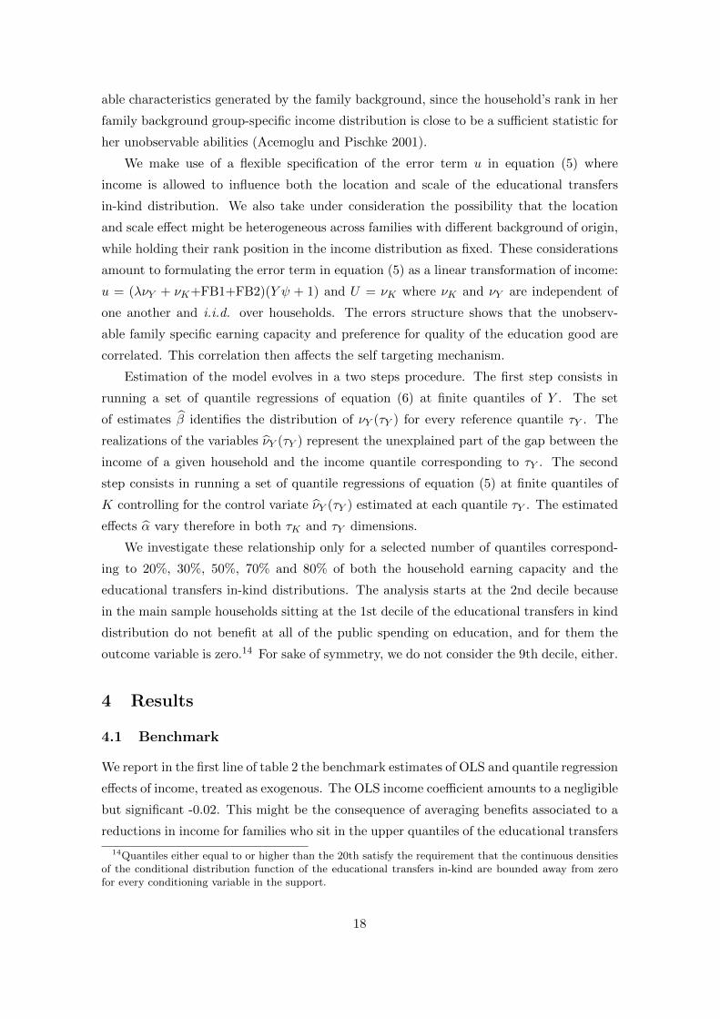
We report in the first line of table 2 the benchmark estimates of OLS and quantile regression

effects of income, treated as exogenous. The OLS income coefficient amounts to a negligible

but significant -0.02. This might be the consequence of averaging benefits associated to a

reductions in income for families who sit in the upper quantiles of the educational transfers

14Quantiles either equal to or higher than the 20th satisfy the requirement that the continuous densitiesof the conditional distribution function of the educational transfers in-kind are bounded away from zerofor every conditioning variable in the support.

18

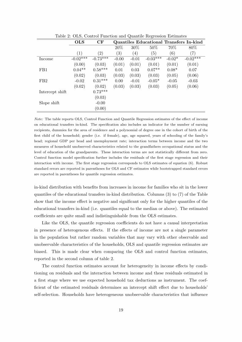
Table 2: OLS, Control Function and Quantile Regression Estimates

OLS CF Quantiles Educational Transfers In-kind20% 30% 50% 70% 80%

(1) (2) (3) (4) (5) (6) (7)

Income -0.02*** -0.73*** -0.00 -0.01 -0.03*** -0.02* -0.02***(0.00) (0.03) (0.01) (0.01) (0.01) (0.01) (0.01)

FB1 0.04** 0.58*** 0.01 0.03 0.07** 0.08* 0.07(0.02) (0.03) (0.03) (0.03) (0.03) (0.05) (0.06)

FB2 -0.02 0.31*** 0.00 -0.01 -0.05* -0.05 -0.03(0.02) (0.02) (0.03) (0.03) (0.03) (0.05) (0.06)

Intercept shift 0.73***(0.03)

Slope shift -0.00(0.00)

Note: The table reports OLS, Control Function and Quantile Regression estimates of the effect of income

on educational transfers in-kind. The specification also includes an indicator for the number of earning

recipients, dummies for the area of residence and a polynomial of degree one in the cohort of birth of the

first child of the household; gender (i.e. if female), age, age squared, years of schooling of the family’s

head; regional GDP per head and unemployment rate; interaction terms between income and the two

measures of household unobserved characteristics related to the grandfathers occupational status and the

level of education of the grandparents. These interaction terms are not statistically different from zero.

Control function model specification further includes the residuals of the first stage regression and their

interaction with income. The first stage regression corresponds to OLS estimates of equation (6). Robust

standard errors are reported in parentheses for OLS and CF estimates while bootstrapped standard errors

are reported in parentheses for quantile regression estimates.

in-kind distribution with benefits from increases in income for families who sit in the lower

quantiles of the educational transfers in-kind distribution. Columns (3) to (7) of the Table

show that the income effect is negative and significant only for the higher quantiles of the

educational transfers in-kind (i.e. quantiles equal to the median or above). The estimated

coefficients are quite small and indistinguishable from the OLS estimates.

Like the OLS, the quantile regression coefficients do not have a causal interpretation

in presence of heterogenous effects. If the effects of income are not a single parameter

in the population but rather random variables that may vary with other observable and

unobservable characteristics of the households, OLS and quantile regression estimates are

biased. This is made clear when comparing the OLS and control function estimates,

reported in the second column of table 2.

The control function estimates account for heterogeneity in income effects by condi-

tioning on residuals and the interaction between income and these residuals estimated in

a first stage where we use expected household tax deductions as instrument. The coef-

ficient of the estimated residuals determines an intercept shift effect due to households’

self-selection. Households have heterogeneous unobservable characteristics that influence

19

permanently the amount of educational transfers in-kind received by affecting the intercept

of the educational transfers in-kind equation. The interaction term captures, instead, the

slope shift effect on the marginal effect of income on the amount of the educational transfers

in-kind which is associated to the unobservable heterogeneity in household characteristics.

This interaction term, however, is not statistically significant.

Under plausible assumptions,15 the coefficient of the income variable of the control

function estimates retrieves the average marginal treatment effect in the population. The

control function can be conceived as an average structural relation that provides the

counter-factual conditional expectations of k given y (and other covariates) if y could

be manipulated independently of the errors as if the endogeneity of y was absent (Blundell

and Powell 2003). This average marginal treatment effect in the population, −0.73, is

much higher (in absolute values) than the corresponding OLS estimate and represents

the average marginal effect of income if the latter would be perfectly observable by the

governments (i.e. if the income would be exogenous).

Although CF method considers both the intercept-slope shift assumptions on the way

that covariates are allowed to influence the conditional distributions of the endogenous

variables, it offers only a conditional mean view of the structural relationship. Structural

quantile treatment effect estimation broadens this view, offering a more complete charac-

terization of the stochastic relationship among income and educational transfers in-kind.

4.2 First stage

Table 3 reports quantile estimates of equation (6) for the main sample and for two sub-

samples used in the analyses that will follow. We interpret the estimated coefficients as

the sum of two effects through which a change in our instrument exogenously manipulate

the distribution of income Y . Let yN be the net of taxes income, that is, by definition,

equal to the gross income yG minus the personal income tax liability T and T = t(yG−d),

where t represents the average tax rate and d a tax deduction. We can decompose the

overall effect of a change of (expected) tax deductions on net of taxes income as follows:

∂yN∂d

= t′ +∂yG∂d

(1− t′)

where t′ stands for marginal personal income tax rate.

As a consequence, the variation of (net of taxes) income due to a one euro increase of

(expected) tax deductions is the sum of the tax cut equal to the marginal tax rate (the

direct effect), and of the variation of the gross income net of the marginal tax rate (the

15Our two measures of unobservable household characteristics related to the grandfathers occupationalconditions and grandparents’ level of education and other household specific heterogeneity componentsunrelated to these two family background variables are all mean independent of the instrument z in sucha way that the instrument is as good as randomly assigned.

20

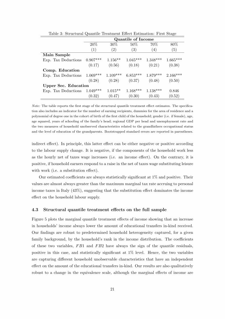
Table 3: Structural Quantile Treatment Effect Estimation: First Stage

Quantile of Income20% 30% 50% 70% 80%(1) (2) (3) (4) (5)

Main SampleExp. Tax Deductions 0.907*** 1.156** 1.045*** 1.348*** 1.665***

(0.17) (0.56) (0.18) (0.21) (0.38)Comp. EducationExp. Tax Deductions 1.069*** 1.109*** 6.853*** 1.879*** 2.166***

(0.28) (0.28) (0.37) (0.48) (0.50)Upper Sec. EducationExp. Tax Deductions 1.049*** 1.015** 1.168*** 1.138*** 0.846

(0.32) (0.47) (0.30) (0.43) (0.52)

Note: The table reports the first stage of the structural quantile treatment effect estimates. The specifica-

tion also includes an indicator for the number of earning recipients, dummies for the area of residence and a

polynomial of degree one in the cohort of birth of the first child of the household; gender (i.e. if female), age,

age squared, years of schooling of the family’s head; regional GDP per head and unemployment rate and

the two measures of household unobserved characteristics related to the grandfathers occupational status

and the level of education of the grandparents. Bootstrapped standard errors are reported in parentheses.

indirect effect). In principle, this latter effect can be either negative or positive according

to the labour supply change. It is negative, if the components of the household work less

as the hourly net of taxes wage increases (i.e. an income effect). On the contrary, it is

positive, if household earners respond to a raise in the net of taxes wage substituting leisure

with work (i.e. a substitution effect).

Our estimated coefficients are always statistically significant at 1% and positive. Their

values are almost always greater than the maximum marginal tax rate accruing to personal

income taxes in Italy (43%), suggesting that the substitution effect dominates the income

effect on the household labour supply.

4.3 Structural quantile treatment effects on the full sample

Figure 5 plots the marginal quantile treatment effects of income showing that an increase

in households’ income always lower the amount of educational transfers in-kind received.

Our findings are robust to predetermined household heterogeneity captured, for a given

family background, by the household’s rank in the income distribution. The coefficients

of these two variables, FB1 and FB2 have always the sign of the quantile residuals,

positive in this case, and statistically significant at 1% level. Hence, the two variables

are capturing different household unobservable characteristics that have an independent

effect on the amount of the educational transfers in-kind. Our results are also qualitatively

robust to a change in the equivalence scale, although the marginal effects of income are

21

Figure 5: Marginal Quantile Treatment Effects of Income

Note: The figure plots the marginal quantile treatment effects of income for a given quantile of the household

earning capacity. These marginal quantile treatment effects are calculated taking also into account the

scale shift effect, measured by the interaction between income and the residuals of the given quantile of

the household earning capacity, and the interactions between income and our two measures of household

unobserved characteristics related to the grandfathers occupational status and the level of education of the

grandparents, each of them considered separately. Confidence bands at 99% level.

less heterogeneous.16

4.3.1 Fixing quantiles of the household earning capacity, τY

A one euro increase in income reduces the amount of educational transfers in-kind more

at the 80th quantile than at the 20th quantile of the K distribution. Table 4, panel (a),

shows a battery of tests for the homogeneity of these marginal effects. The equality of

the effects is rejected, in some cases at 10% level of significance, at all quantiles of the

household earning capacity with the exception of the median. We interpret our findings

as evidence that the opting out for private schools is higher for those households who

value most the quality of the education good since sitting at the higher quantiles of the

educational transfers in-kind distribution.17

16These results are reported in appendix C.17We could have also compared other quantiles, for instance either the lowest and the median or the

median and the highest. However, since in our case, the relationship of interest is almost monotone,heterogeneity of the effects is fully described by our Table 4 that compares the lowest and the highestquantiles.

22

Table 4: Homogeneity Tests: 20th and 80th quantiles of K fixing τYPanel (a): 20th and 80th quantiles of K, given τYτY : 20% τY : 30% τY : 50% τY : 70% τY : 80%

MQTEY 0.184* 0.149** 0.166 0.133** 0.108**(0.10) (0.07) (0.31) (0.06) (0.05)

Panel (b): 20th and 80th quantiles of Y, given τKτK : 20% τK : 30% τK : 50% τK : 70% τK : 80%

MQTEY -0.570*** -0.613*** -0.604*** -0.624*** -0.647***(0.11) (0.08) (0.07) (0.07) (0.06)

Note: The Table reports the homogeneity tests of marginal quantile treatment effects of income, in the main

sample, at the 20th and the 80th quantiles of educational transfers in-kind distribution, fixing quantiles of

the household earning capacity (panel (a)) and at the 20th and the 80th quantiles of the household earning

capacity, fixing quantiles of the educational transfers in-kind distribution (panel (b)). Standard errors are

reported in parentheses.

4.3.2 Fixing quantiles of the household preferences for quality, τK

Panel (b) of Table 4 reports the homogeneity test between the marginal effects of income

at the 20th and the 80th quantiles of the household earning capacity. These differences

are always negative and statistically significant at a 1% level, suggesting that a one euro

increase in income reduces more the amount of educational transfers in-kind for the 20th

quantile than for the 80th quantile of the household earning capacity. The marginal effect

of income, if negative, can be interpreted in terms of a marginal benefit rate. Our income

coefficients are, for instance, 1.437 and 0.79 for the 20th and 80 quantiles of the household

earning capacity. This is evidence of the progressivity of the educational transfers in-kind

since their benefit rate is decreasing, in absolute values, although not strictly monotonically

in our case, in the income distribution.

4.3.3 Mean (quantile) treatment effects

The structural quantile treatment effect method allows to decompose the stochastic effect

of the distribution of income on the distribution of the educational transfers in-kind into

two distinct dimensions: the one related to the distribution of the household earning ca-

pacity and the one related to the distribution of the educational transfers in-kind proxing

household preferences for the quality of the education good. Our assumption on the errors

structure has provided structural insights into how these two dimensions are connected.

As suggested by Ma and Koenker (2006), there are other relevant but more aggregated

evaluation parameters that can be retrieved from structural quantile treatment effects esti-

mation. The mean quantile treatment effect is obtained by integrating out the distribution

of the household earning capacity, while the mean treatment effect results from averaging

again, this time with respect to the quantiles of the distribution of the educational trans-

23

Figure 6: Average Quantile Treatment Effects of Income

Note: The figure plots the average quantile treatment effects, the mean treatment effect and the mean

(average) treatment of income using control function method reported in Table 2. The mean treatment

effect is calculated integrating out the distribution of the household earning capacity by assigning as weights

the area under the distribution evaluated at the fix points of the 20th, 30th, 50th, 70th and 80th quantiles.

The 20th bottom and upper part of the distribution are assumed to a have a weight equal to zero. The

mean (average) treatment effect is obtained by averaging across the quantiles of the distribution of the

educational transfers in-kind. Confidence bands at 99% level.

fers in-kind. The mean treatment effect theoretically coincides with what is estimated by

the two-stage least-squares estimator in the pure location shift version of the model and

might correspond to the average treatment effect estimated in section 4.1 using the control

function method. Figure 6 supports our argument. The difference between the average

treatment effect retrieved in control function CF and the mean treatment effect obtained

starting from our structural quantile treatment effect estimates is likely to be due to our

hypothesis on assigning a zero weight to the 20th and 80th quantiles of the distributions of

the household earning capacity and the amount of educational transfers in-kind to compute

the final effect.

4.4 Analysis across educational levels

The Besley and Coate (1991) model chiefly applies to compulsory education, where enrol-

ment is mandatory to all children and parents only have to choose the type, private or

public, of the school. The households’ choice for post-compulsory education is, instead, se-

quential. First, the household decides whether or not to enroll the child at school. Only in

24

the event that the kid attends post-compulsory education, the household chooses between

private and public education.

Furthermore, the two stages of the education system can be further differentiated

according to the quality of the educational services they offer. Based on the Italian ex-

perience, Bertola et al. (2007) and Bertola and Checchi (2013) show that the quality of

private schooling for upper secondary is lower than that related to public schools, inferring

the “remedial role” played by upper secondary private education. To account for both

these issues, this section deals with replicating our main analysis for two subsamples that

distinguish between families with children in compulsory schooling age and those with kids

in upper secondary schooling age. Additional tables with robustness checks are reported

in the appendix.

4.4.1 Compulsory education

Panel (a) of figure 7 illustrates the marginal effect of income on the amount of educational

transfers in-kind when we consider only families with at least one child in compulsory

schooling age.18 Estimates are based on a reduced sample of 888 households. We find

that an increase in income affects positively the amount of educational transfers in-kind

at the 20th and 30th quantiles of the K distribution but negatively at quantiles above the

median.

The marginal impact of income on the median amount of educational transfers in-kind

is negligible. At the lower quantiles of the educational transfers in-kind, this effect is low

and, for a given earning capacity of the households, only families that value less the quality

of the educational services consume the publicly provided education good. Since quality is

a normal good, the marginal effect of an increase in income on the amount of educational

transfers in-kind is positive for them.

At higher quantiles of the educational transfers in-kind, households who value more

the quality of the education good self-target themselves by opting out, gradually, towards

private education. For this reason, at the higher quantiles of the educational transfers in-

kind distribution, the sign of the marginal effect of income on the amount of educational

transfers in-kind is negative. The differences in the marginal effect of income at the 20th

and 80th quantiles of the educational transfers in-kind are higher at the lower quantiles

of the household earning capacity. The households who value less the quality of the edu-

cational services and have a lower earning capacity are those who benefit more from the

publicly provided mandatory education system.

Figure 7 provides also evidence of the progressivity of the educational transfers in-

18Here we are not considering families with children at kindergarten. This is because kindergarten isnot compulsory in Italy. Results are qualitatively robust when we consider kindergarten. These results arereported in appendix C.

25

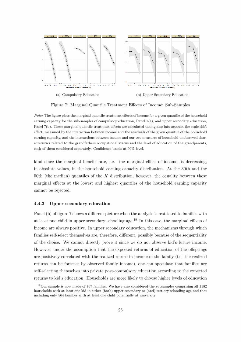
(a) Compulsory Education (b) Upper Secondary Education

Figure 7: Marginal Quantile Treatment Effects of Income: Sub-Samples

Note: The figure plots the marginal quantile treatment effects of income for a given quantile of the household

earning capacity for the sub-samples of compulsory education, Panel 7(a), and upper secondary education,

Panel 7(b). These marginal quantile treatment effects are calculated taking also into account the scale shift

effect, measured by the interaction between income and the residuals of the given quantile of the household

earning capacity, and the interactions between income and our two measures of household unobserved char-

acteristics related to the grandfathers occupational status and the level of education of the grandparents,

each of them considered separately. Confidence bands at 99% level.

kind since the marginal benefit rate, i.e. the marginal effect of income, is decreasing,

in absolute values, in the household earning capacity distribution. At the 30th and the

50th (the median) quantiles of the K distribution, however, the equality between these

marginal effects at the lowest and highest quantiles of the household earning capacity

cannot be rejected.

4.4.2 Upper secondary education

Panel (b) of figure 7 shows a different picture when the analysis is restricted to families with

at least one child in upper secondary schooling age.19 In this case, the marginal effects of

income are always positive. In upper secondary education, the mechanisms through which

families self-select themselves are, therefore, different, possibly because of the sequentiality

of the choice. We cannot directly prove it since we do not observe kid’s future income.

However, under the assumption that the expected returns of education of the offsprings

are positively correlated with the realized return in income of the family (i.e. the realized

returns can be forecast by observed family income), one can speculate that families are

self-selecting themselves into private post-compulsory education according to the expected

returns to kid’s education. Households are more likely to choose higher levels of education

19Our sample is now made of 767 families. We have also considered the subsamples comprising all 1182households with at least one kid in either (both) upper secondary or (and) tertiary schooling age and thatincluding only 564 families with at least one child potentially at university.

26

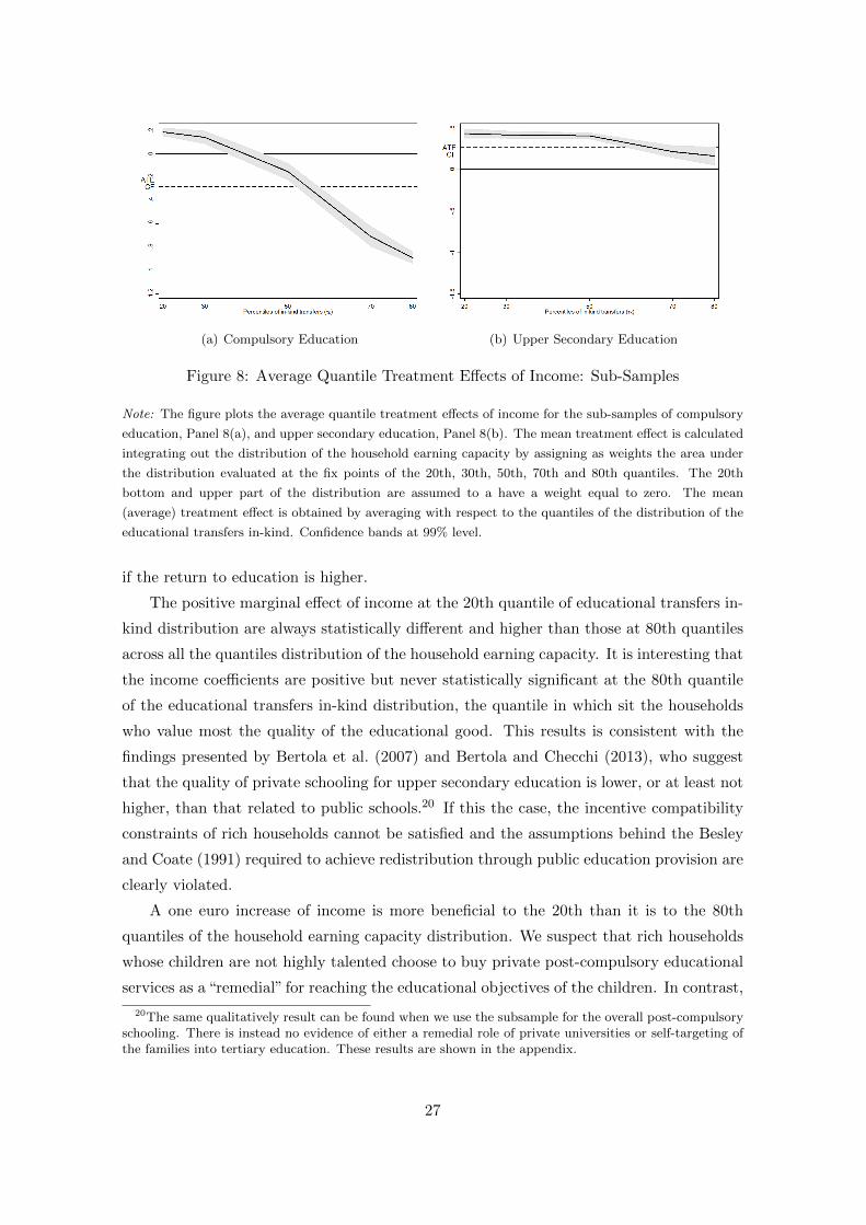
(a) Compulsory Education (b) Upper Secondary Education

Figure 8: Average Quantile Treatment Effects of Income: Sub-Samples

Note: The figure plots the average quantile treatment effects of income for the sub-samples of compulsory

education, Panel 8(a), and upper secondary education, Panel 8(b). The mean treatment effect is calculated

integrating out the distribution of the household earning capacity by assigning as weights the area under

the distribution evaluated at the fix points of the 20th, 30th, 50th, 70th and 80th quantiles. The 20th

bottom and upper part of the distribution are assumed to a have a weight equal to zero. The mean

(average) treatment effect is obtained by averaging with respect to the quantiles of the distribution of the

educational transfers in-kind. Confidence bands at 99% level.

if the return to education is higher.

The positive marginal effect of income at the 20th quantile of educational transfers in-

kind distribution are always statistically different and higher than those at 80th quantiles

across all the quantiles distribution of the household earning capacity. It is interesting that

the income coefficients are positive but never statistically significant at the 80th quantile

of the educational transfers in-kind distribution, the quantile in which sit the households

who value most the quality of the educational good. This results is consistent with the

findings presented by Bertola et al. (2007) and Bertola and Checchi (2013), who suggest

that the quality of private schooling for upper secondary education is lower, or at least not

higher, than that related to public schools.20 If this the case, the incentive compatibility

constraints of rich households cannot be satisfied and the assumptions behind the Besley

and Coate (1991) required to achieve redistribution through public education provision are

clearly violated.

A one euro increase of income is more beneficial to the 20th than it is to the 80th

quantiles of the household earning capacity distribution. We suspect that rich households

whose children are not highly talented choose to buy private post-compulsory educational

services as a “remedial” for reaching the educational objectives of the children. In contrast,

20The same qualitatively result can be found when we use the subsample for the overall post-compulsoryschooling. There is instead no evidence of either a remedial role of private universities or self-targeting ofthe families into tertiary education. These results are shown in the appendix.

27

kids coming from the poor household that are not talented should stop studying since for

them the opportunity costs of attending schools is too high. It follows for upper secondary

education, that public schools should attract proportionally more skilled individuals, both

from rich and poor households, as shown by Bertola et al. (2007).

Panels (a) and (b) of figure 8 plot the average quantile treatment effects and the av-

erage treatment effects for compulsory and upper secondary education. These parameters

are retrieved from our structural quantile treatment effects estimates integrating over the

two relevant dimensions, the household earning capacity and the educational transfers in-

kind distributions. In both cases the average treatment effects almost coincide with the

parameters estimated using control function method. Consequently, on average, public

education provision is redistributive for compulsory education but it is not redistributive

for post-compulsory education.

5 Conclusions

This paper investigated the mechanisms behind the redistributiveness of public educa-

tion provision using Italian data. We interpret almost free public educational services as

transfers in-kind received by families who do not choose private education. The monetary

equivalent value of the transfers in-kind is measured by the expected cost supported by the

government to provide the service for free, reflecting the quality of the service provided.

We show that an increase in income reduces the amount of educational transfers in-

kind (i) more for higher quantiles of the educational transfers in-kind (ii) more for lower

quantiles of the household earning capacity. We interpret our results as evidence of a

self-targeting device through which rich households sort themselves into private education.

Our results explain how, for compulsory schooling, the households’ sorting into private

education may motivate a government, that aims at redistributing resources from the rich

to the poor, to use public education provision as transfers in-kind.

Our results suggest that reforms of the public education system that aim at chang-

ing the quality of the publicly provided education services might alter the self-targeting

mechanism premises. This does not necessarily implies that such reforms would lead to

a loss in either efficiency or equity terms. In their conclusions, Besley and Coate (1991),

underline that public education provision will not necessarily be part of an optimal de-

signed redistributional package. The deadweight loss associated with universal education

provision suggests that the same distributional goals could be achieved more efficiently

through other feasible policies. There is a clear trade-off between the cost to the govern-

ment to minimize the asymmetric information on the households’ earning capacity and the

deadweight loss inherent in an inefficient quality of the public provision of education. The

higher the cost to the government of observing its citizens’ earning capacity the higher the

28

necessity of an inefficient self-targeting device.

The empirical investigation shows that different self-selection processes apply at upper

secondary education level where there also is evidence of a violation of one of the main

assumption behind the self-targeting mechanism. On the one hand, for post-compulsory

education families sort themselves according to the expected returns to kid’s education. On

the other hand, we find that the marginal effect of income is never statistically significant

at the 80th quantile of the educational transfers in-kind distribution, the quantile in which

sit the households who value most the quality of the educational good. This result suggests

that the quality of private schooling for upper secondary education, is lower or at least

not higher than that related to public schools as a consequence of the demand of less

talented kids coming from rich households as also proved by Bertola et al. (2007) and

Bertola and Checchi (2013). If this is the case, the incentive compatibility constraints of

rich households cannot be satisfied since the quality of the publicly provided education

good is not lower than that characterizing the private schools. Since only talented children

coming from poor households do not stop studying and they are enrolled at public schools,

for upper secondary education, public schools should attract proportionally more skilled

individuals. Nevertheless, public education is not redistributive since for poor household

with less talented kids the opportunity cost school of attending schools is too high.

29

References

Aaberge, R., Bhuller, M., Langørgen, A. and Mogstad, M. (2010). The distributional im-pact of public services when needs differ, Journal of Public Economics 94(9-10): 549–562.

Aaberge, R., Langorgen, A. and Lindgren, P. (2013). The distributional impact of publicservices in european countries

”476.

Acemoglu, D. and Pischke, J. S. (2001). Changes in the wage structure, family income,and children’s education, European Economic Review 45(4-6): 890–904.

Asquini, G. and Bettoni, C. (eds) (2003). Analisi delle spese per istruzione, Franco Angeli.

Bertola, G. and Checchi, D. (2013). Who chooses which private education? theory andinternational evidence, LABOUR 27(3): 249–271.

Bertola, G., Checchi, D. and Oppedisano, V. (2007). Private school quality in italy, Gior-nale degli Economisti 66(3): 375–400.

Besley, T. and Coate, S. (1991). Public provision of private goods and the redistributionof income, American Economic Review 81(4): 979–84.

Blackorby, C. and Donaldson, D. (1988). Cash versus kind, self-selection, and efficienttransfers, American Economic Review 78(4): 691–700.

Blundell, R. and Powell, J. (2003). Endogeneity in nonparametric and semiparametricregression models, in L. H. M. Dewatripont and e. S.J. Turnovsky (eds), Advancesin Economics and Econonometrics: Theory and Applications, Vol. II, Eighth WorldCongress, Cambridge: Cambridge University Press.

Checchi, D. and Jappelli, T. (2003). School choice and quality, IZA Discussion Papers828, Institute for the Study of Labor (IZA).

Checchi, D. and Jappelli, T. (2007). The impact of perceived public school quality onprivate school choice in italy, in L. Woessman and e. Petersen, P. (eds), Schools andthe equal of opportunity problem, MIT.

Currie, J. and Gahvari, F. (2008). Transfers in cash and in-kind: Theory meets the data,Journal of Economic Literature 46(2): 333–83.

Fershtman, C., Murphy, K. M. and Weiss, Y. (1996). Social status, education, and growth,Journal of Political Economy 104(1): 108–32.

Gahvari, F. and Mattos, E. (2007). Conditional cash transfers, public provision of privategoods, and income redistribution, American Economic Review 97(1): 491–502.

INVALSI-MIPA (2005). Aspis iii - linea di ricerca sull’analisi della spesa per istruzione,Technical report, INVALSI-MIPA.

ISTAT (2003). Labour for surv, Technical report, ISTAT.

Koenker, R. and Bassett, Gilbert, J. (1978). Regression quantiles, Econometrica 46(1): pp.33–50.

30

Lefranc, A., Pistolesi, N. and Trannoy, A. (2009). Equality of opportunity and luck:Definitions and testable conditions, with an application to income in France, Journalof Public Economics 93(11-12): 1189 – 1207.

Ma, L. and Koenker, R. (2006). Quantile regression methods for recursive structuralequation models, Journal of Econometrics 134(2): 471 – 506.

Roemer, J. (1998). Equality of Opportunity, Harvard University Press, Cambridge.

Sander, W. (2001). The effects of catholic schools on religiosity, education and competi-tion, Technical report, National Center for the Study of Privatization in Education,Occasional Paper n.32.

Stiglitz, J. E. (1974). The demand for education in public and private school systems,Journal of Public Economics 3(4): 349–385.

31

A Assessing the average costs per student at regional and

educational level

In Italy, the educational public system is managed by local authorities (regions, provinces

and municipalities), although most of the financial resources arises from the central state.

According to INVALSI-MIPA (2005) 71% of the public expenditures for education (from

pre-primary to upper secondary) is financed by the central state, while regions account for

6%, provinces for 5.5% and the remaining, 17.5%, is financed by municipalities. Although

competencies on public education in Italy are spread across several authorities, in this

paper we use regions as the unit of analysis for three main reasons. First, the main source

of variation in educational expenditures in Italy is at the local level, as 95% of the central

government spending on education finances the salaries of the teaching and non teaching

staff. Second, regions (which territory is then organized into provinces and municipalities)

can be considered as ’whole units’ due to the complex system of financial transfers from

higher to lower levels of governments (mainly from regions to province and municipalities).

Third, the only - at the best of our knowledge - detailed analysis on spending on education

carried out in Italy by INVALSI-MIPA (2005) emphasizes the regional (together with the

educational level) dimension, implicitly recognizing a primary source of variation at this

level. Moreover, even within regions there is variation in local government spending across

educational levels that correspond to primary (scuola elementare), compulsory secondary

school (scuole medie inferiori), post-compulsory secondary school (scuole superiori) and

tertiary education. We interpret this region by education level variability as a result of

heterogenous spending priorities on different target (income) groups.

The estimation of the average cost of public education by region and educational level is

a difficult exercise. The Financial Statement (Rendiconto Generale) of the Italian Ministry

of Education (MIUR), a document which records the expenditures on public education, has

an aggregate perspective and the reported figures do not allow to calculate the expenditures

along both dimensions (regions and educational levels) at the same time. However, for all

education levels up to upper secondary school (including then pre-primary and excluding

tertiary education) we take advantage of the results of a unique study named ASPIS III

realised in 2005 (with data referring to 2003) by the Italian National Institute for the

Evaluation of Education System (INVALSI) and the Consortium for the Development of

the Methodologies and Innovations of the Public Administrations (MIPA). This study

draws together information arising from several sources (Ministry of Economy, Ministry

of Education, Italian Institute of Statistics) to develop a matrix of public expenditures

on education based on both the regional and the educational level dimensions. In the

following section we briefly describe the main features of the methodology developed by

ASPIS III. All details (only in Italian) can be found in the accompanying reports Asquini

and Bettoni (2003) and INVALSI-MIPA (2005). Finally, a specific section describes the

methodology followed to estimate the average cost of tertiary education.

A.1 Pre-primary, primary, lower and upper secondary school

The Financial Statement of the Italian Ministry of Education records public spending on

education according to two classifications. One aggregates data at the central government

32

level, distinguishing across different levels of education but not across different regions. The

other organizes data by regions but does not distinguish across different educational levels.

In order to attribute central government expenditures by educational levels to regions and,

viceversa, region-specific expenditures to different educational levels, ASPIS III exploits a

number of so called drivers. Drivers are indicators that depend on the specific expenditure.

For instance, the main driver is represented by the number of students and of teaching and

non teaching staff in each region and educational level. To some extent using as a weighting

factor the number of students and teachers, data provided by ASPIS III are taking account

of differences in quality and efficiency in the public service production across regions and

level of education. A further advantage of using ASPIS III is that data arise from a

consolidated financial statement of central government and local authorities, avoiding the

risk of double counting the value of expenditures which are financed by transfers from

higher to lower levels of government.

ASPIS data provide us with a r × e matrix of data whose cells record the public

spending (total costs) on education for 20 Italian regions (r) and 4 educational levels (e)

for year 2003. We divide each of these total costs by the total number of students enrolled

at school reported in the corresponding cell of an analogue r × e matrix. We end up with

a r× e matrix providing the average spending per student by region and educational level

indicated in the main text as acre.21 We finally apply regional-specific general indexes of

consumer prices to inflate these average costs to 2004.

A.2 Tertiary education

To estimate the average costs of providing public tertiary education in Italy, we adopt a

different strategy. We calculate the overall amount of resources that each Italian university

receives from the central government and the local public authorities from the reclassified

financial statements of Italian public universities (state or regional) provided by CNVSU

for year 2004. This overall amount of resources measures the total costs of producing

tertiary education at university level. The regional total costs are obtained by summing

up total costs accruing to all universities located in a given region. These regional total

costs are then divided by the number of students enrolled in each region to end up with

the average regional costs of providing public tertiary education. Notice that these average

costs are net of the fees paid by households, i.e. they represent the costs actually borne

by the government. We take account of students’ mobility across regions by weighting

each regional average costs by the probability that a student resident in a certain region

is enrolled at a university in a different region. These probabilities are calculated using a

20× 20 students’ mobility matrix based on the enrollment statistics of MIUR.22

21Data estimated are net public expenditures on education, as households’ out-of-pocket payments andother financial sources beyond government are excluded.

22SHIW 2004 data do not provide information on the university attended by the kids. In Italy, generally,students enrolled at a university located in a region other than that of their parents’ residence, use not tochange their residence. In such a case, they would be surveyed by the Bank of Italy within the family.

33

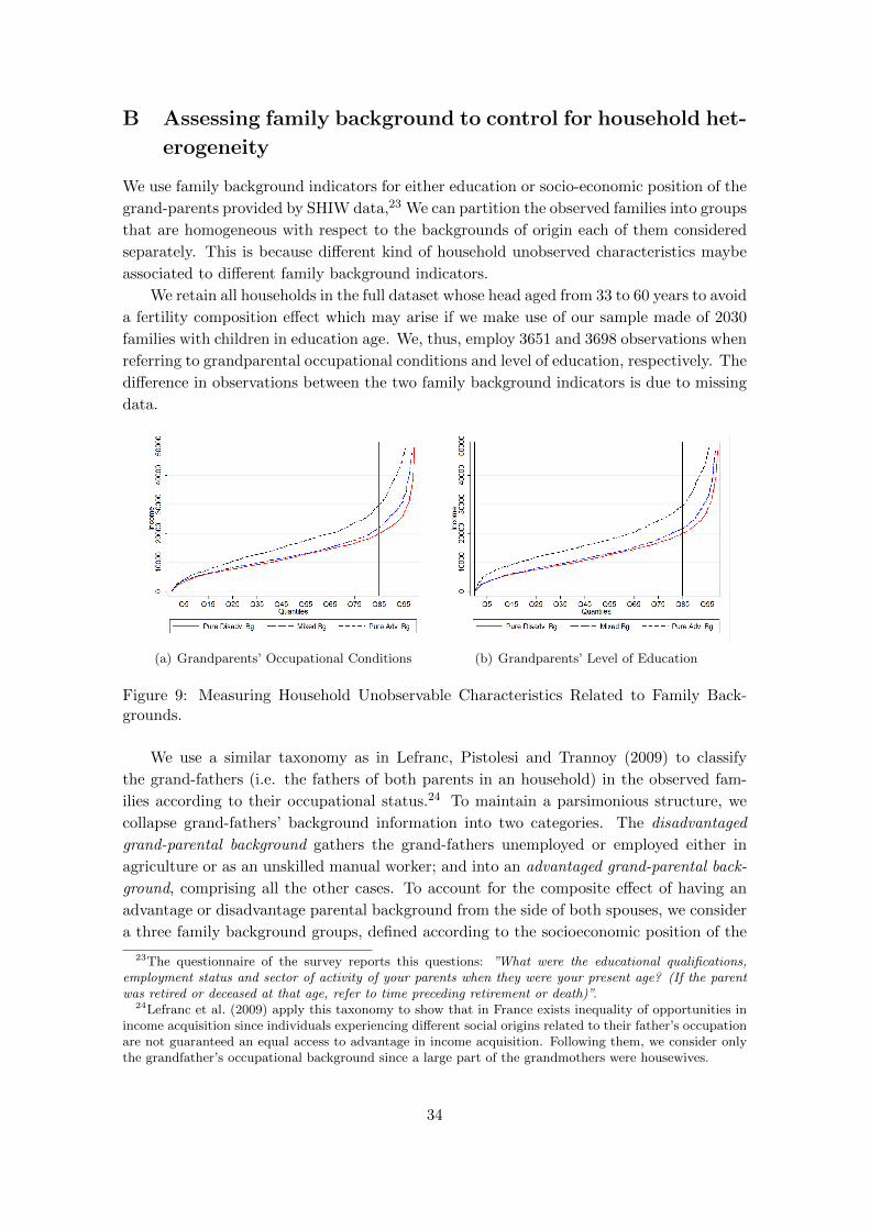
B Assessing family background to control for household het-

erogeneity

We use family background indicators for either education or socio-economic position of the

grand-parents provided by SHIW data,23 We can partition the observed families into groups

that are homogeneous with respect to the backgrounds of origin each of them considered

separately. This is because different kind of household unobserved characteristics maybe

associated to different family background indicators.

We retain all households in the full dataset whose head aged from 33 to 60 years to avoid

a fertility composition effect which may arise if we make use of our sample made of 2030

families with children in education age. We, thus, employ 3651 and 3698 observations when

referring to grandparental occupational conditions and level of education, respectively. The

difference in observations between the two family background indicators is due to missing

data.

(a) Grandparents’ Occupational Conditions (b) Grandparents’ Level of Education

Figure 9: Measuring Household Unobservable Characteristics Related to Family Back-grounds.

We use a similar taxonomy as in Lefranc, Pistolesi and Trannoy (2009) to classify

the grand-fathers (i.e. the fathers of both parents in an household) in the observed fam-

ilies according to their occupational status.24 To maintain a parsimonious structure, we

collapse grand-fathers’ background information into two categories. The disadvantaged

grand-parental background gathers the grand-fathers unemployed or employed either in

agriculture or as an unskilled manual worker; and into an advantaged grand-parental back-

ground, comprising all the other cases. To account for the composite effect of having an

advantage or disadvantage parental background from the side of both spouses, we consider

a three family background groups, defined according to the socioeconomic position of the

23The questionnaire of the survey reports this questions: ”What were the educational qualifications,employment status and sector of activity of your parents when they were your present age? (If the parentwas retired or deceased at that age, refer to time preceding retirement or death)”.

24Lefranc et al. (2009) apply this taxonomy to show that in France exists inequality of opportunities inincome acquisition since individuals experiencing different social origins related to their father’s occupationare not guaranteed an equal access to advantage in income acquisition. Following them, we consider onlythe grandfather’s occupational background since a large part of the grandmothers were housewives.

34

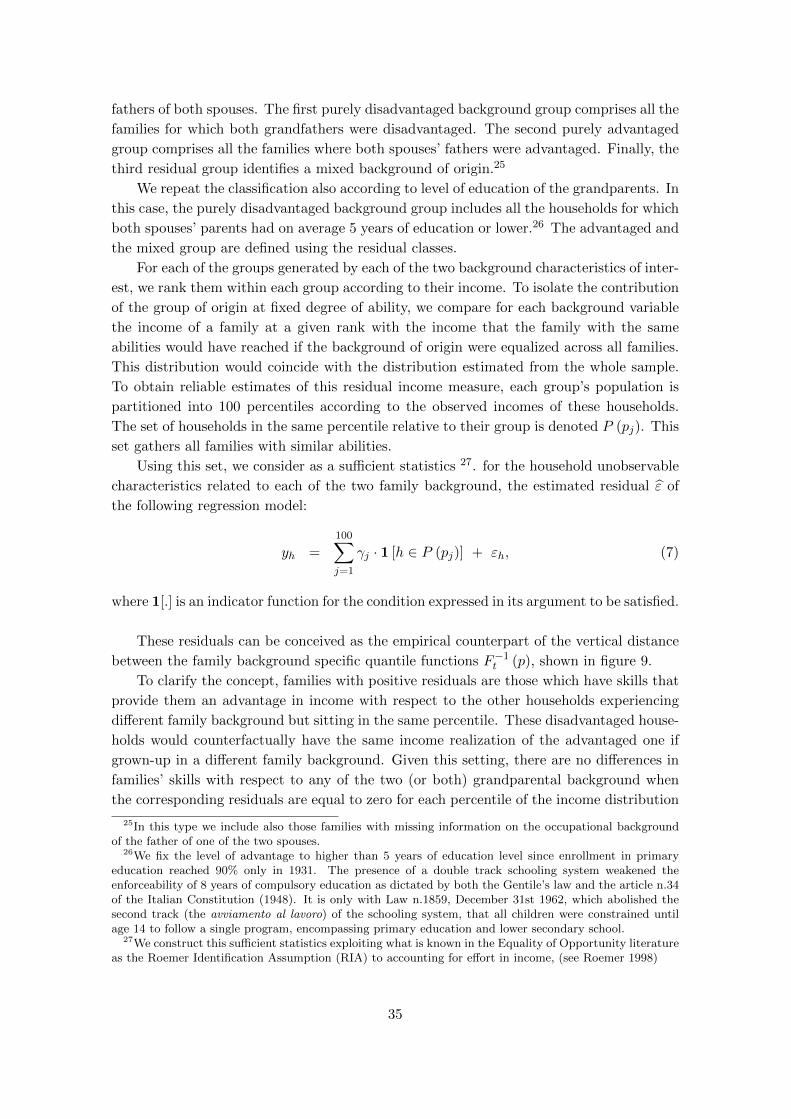
fathers of both spouses. The first purely disadvantaged background group comprises all the

families for which both grandfathers were disadvantaged. The second purely advantaged

group comprises all the families where both spouses’ fathers were advantaged. Finally, the

third residual group identifies a mixed background of origin.25

We repeat the classification also according to level of education of the grandparents. In

this case, the purely disadvantaged background group includes all the households for which

both spouses’ parents had on average 5 years of education or lower.26 The advantaged and

the mixed group are defined using the residual classes.

For each of the groups generated by each of the two background characteristics of inter-

est, we rank them within each group according to their income. To isolate the contribution

of the group of origin at fixed degree of ability, we compare for each background variable

the income of a family at a given rank with the income that the family with the same

abilities would have reached if the background of origin were equalized across all families.

This distribution would coincide with the distribution estimated from the whole sample.

To obtain reliable estimates of this residual income measure, each group’s population is

partitioned into 100 percentiles according to the observed incomes of these households.

The set of households in the same percentile relative to their group is denoted P (pj). This

set gathers all families with similar abilities.

Using this set, we consider as a sufficient statistics 27. for the household unobservable

characteristics related to each of the two family background, the estimated residual ε̂ of

the following regression model:

yh =

100∑j=1

γj · 1 [h ∈ P (pj)] + εh, (7)

where 1[.] is an indicator function for the condition expressed in its argument to be satisfied.

These residuals can be conceived as the empirical counterpart of the vertical distance

between the family background specific quantile functions F−1t (p), shown in figure 9.

To clarify the concept, families with positive residuals are those which have skills that

provide them an advantage in income with respect to the other households experiencing

different family background but sitting in the same percentile. These disadvantaged house-

holds would counterfactually have the same income realization of the advantaged one if

grown-up in a different family background. Given this setting, there are no differences in

families’ skills with respect to any of the two (or both) grandparental background when

the corresponding residuals are equal to zero for each percentile of the income distribution

25In this type we include also those families with missing information on the occupational backgroundof the father of one of the two spouses.

26We fix the level of advantage to higher than 5 years of education level since enrollment in primaryeducation reached 90% only in 1931. The presence of a double track schooling system weakened theenforceability of 8 years of compulsory education as dictated by both the Gentile’s law and the article n.34of the Italian Constitution (1948). It is only with Law n.1859, December 31st 1962, which abolished thesecond track (the avviamento al lavoro) of the schooling system, that all children were constrained untilage 14 to follow a single program, encompassing primary education and lower secondary school.

27We construct this sufficient statistics exploiting what is known in the Equality of Opportunity literatureas the Roemer Identification Assumption (RIA) to accounting for effort in income, (see Roemer 1998)

35

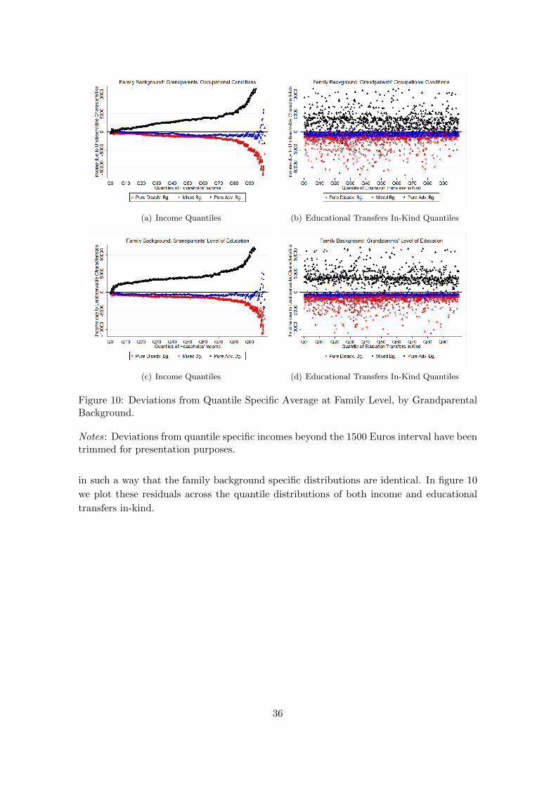
(a) Income Quantiles (b) Educational Transfers In-Kind Quantiles

(c) Income Quantiles (d) Educational Transfers In-Kind Quantiles

Figure 10: Deviations from Quantile Specific Average at Family Level, by GrandparentalBackground.

Notes: Deviations from quantile specific incomes beyond the 1500 Euros interval have beentrimmed for presentation purposes.

in such a way that the family background specific distributions are identical. In figure 10

we plot these residuals across the quantile distributions of both income and educational

transfers in-kind.

36

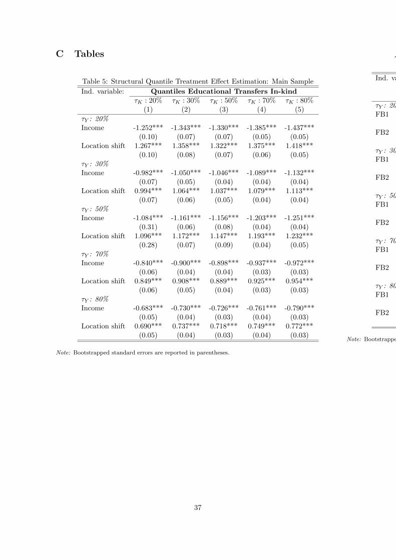
C Tables

Table 5: Structural Quantile Treatment Effect Estimation: Main Sample

Ind. variable: Quantiles Educational Transfers In-kindτK : 20% τK : 30% τK : 50% τK : 70% τK : 80%

(1) (2) (3) (4) (5)

τY : 20%Income -1.252*** -1.343*** -1.330*** -1.385*** -1.437***

(0.10) (0.07) (0.07) (0.05) (0.05)Location shift 1.267*** 1.358*** 1.322*** 1.375*** 1.418***

(0.10) (0.08) (0.07) (0.06) (0.05)τY : 30%Income -0.982*** -1.050*** -1.046*** -1.089*** -1.132***

(0.07) (0.05) (0.04) (0.04) (0.04)Location shift 0.994*** 1.064*** 1.037*** 1.079*** 1.113***

(0.07) (0.06) (0.05) (0.04) (0.04)τY : 50%Income -1.084*** -1.161*** -1.156*** -1.203*** -1.251***

(0.31) (0.06) (0.08) (0.04) (0.04)Location shift 1.096*** 1.172*** 1.147*** 1.193*** 1.232***

(0.28) (0.07) (0.09) (0.04) (0.05)τY : 70%Income -0.840*** -0.900*** -0.898*** -0.937*** -0.972***

(0.06) (0.04) (0.04) (0.03) (0.03)Location shift 0.849*** 0.908*** 0.889*** 0.925*** 0.954***

(0.06) (0.05) (0.04) (0.03) (0.03)τY : 80%Income -0.683*** -0.730*** -0.726*** -0.761*** -0.790***

(0.05) (0.04) (0.03) (0.04) (0.03)Location shift 0.690*** 0.737*** 0.718*** 0.749*** 0.772***

(0.05) (0.04) (0.03) (0.04) (0.03)

Note: Bootstrapped standard errors are reported in parentheses.

Table 23: Structural Quantile Treatment Effect EstimationPost Compulsory Education

Ind. variable: Quantiles Educational Transfers In-kindτK : 20% τK : 30% τK : 50% τK : 70% τK : 80%

(1) (2) (3) (4) (5)

τY : 20%FB1 -0.111 -0.222*** -0.175*** -0.012 0.081

(0.09) (0.07) (0.05) (0.07) (0.08)FB2 -0.045 -0.050 -0.056 0.043 0.060

(0.07) (0.05) (0.04) (0.05) (0.07)τY : 30%FB1 -0.122 -0.256*** -0.210*** -0.016 0.091

(0.10) (0.08) (0.06) (0.07) (0.09)FB2 -0.030 -0.010 -0.023 0.047 0.053

(0.06) (0.05) (0.04) (0.05) (0.06)τY : 50%FB1 -0.138 -0.252*** -0.211*** -0.019 0.091

(0.10) (0.08) (0.06) (0.07) (0.09)FB2 -0.046 -0.034 -0.046 0.046 0.061

(0.06) (0.05) (0.04) (0.05) (0.06)τY : 70%FB1 -0.094 -0.172*** -0.137** -0.015 0.069

(0.09) (0.07) (0.05) (0.06) (0.07)FB2 -0.047 -0.040 -0.050 0.043 0.063

(0.06) (0.05) (0.04) (0.05) (0.07)τY : 80%FB1 -0.092 -0.183*** -0.140*** -0.015 0.070

(0.08) (0.06) (0.05) (0.06) (0.07)FB2 -0.044 -0.031 -0.043 0.043 0.064

(0.06) (0.06) (0.04) (0.05) (0.06)

Note: Bootstrapped standard errors are reported in parentheses.

37

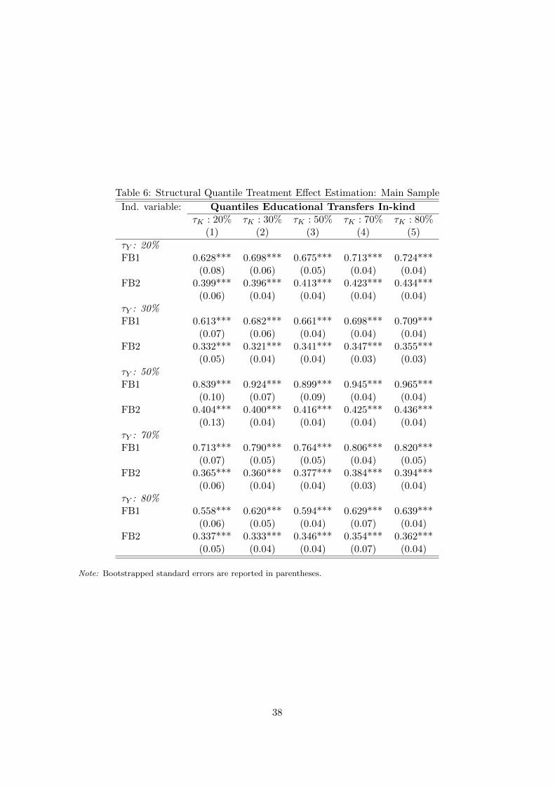
Table 6: Structural Quantile Treatment Effect Estimation: Main Sample

Ind. variable: Quantiles Educational Transfers In-kindτK : 20% τK : 30% τK : 50% τK : 70% τK : 80%

(1) (2) (3) (4) (5)

τY : 20%FB1 0.628*** 0.698*** 0.675*** 0.713*** 0.724***

(0.08) (0.06) (0.05) (0.04) (0.04)FB2 0.399*** 0.396*** 0.413*** 0.423*** 0.434***

(0.06) (0.04) (0.04) (0.04) (0.04)τY : 30%FB1 0.613*** 0.682*** 0.661*** 0.698*** 0.709***

(0.07) (0.06) (0.04) (0.04) (0.04)FB2 0.332*** 0.321*** 0.341*** 0.347*** 0.355***

(0.05) (0.04) (0.04) (0.03) (0.03)τY : 50%FB1 0.839*** 0.924*** 0.899*** 0.945*** 0.965***

(0.10) (0.07) (0.09) (0.04) (0.04)FB2 0.404*** 0.400*** 0.416*** 0.425*** 0.436***

(0.13) (0.04) (0.04) (0.04) (0.04)τY : 70%FB1 0.713*** 0.790*** 0.764*** 0.806*** 0.820***

(0.07) (0.05) (0.05) (0.04) (0.05)FB2 0.365*** 0.360*** 0.377*** 0.384*** 0.394***

(0.06) (0.04) (0.04) (0.03) (0.04)τY : 80%FB1 0.558*** 0.620*** 0.594*** 0.629*** 0.639***

(0.06) (0.05) (0.04) (0.07) (0.04)FB2 0.337*** 0.333*** 0.346*** 0.354*** 0.362***

(0.05) (0.04) (0.04) (0.07) (0.04)

Note: Bootstrapped standard errors are reported in parentheses.

38

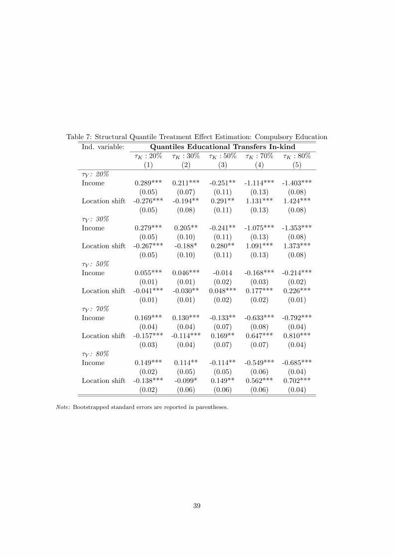
Table 7: Structural Quantile Treatment Effect Estimation: Compulsory Education

Ind. variable: Quantiles Educational Transfers In-kindτK : 20% τK : 30% τK : 50% τK : 70% τK : 80%

(1) (2) (3) (4) (5)

τY : 20%Income 0.289*** 0.211*** -0.251** -1.114*** -1.403***

(0.05) (0.07) (0.11) (0.13) (0.08)Location shift -0.276*** -0.194** 0.291** 1.131*** 1.424***

(0.05) (0.08) (0.11) (0.13) (0.08)τY : 30%Income 0.279*** 0.205** -0.241** -1.075*** -1.353***

(0.05) (0.10) (0.11) (0.13) (0.08)Location shift -0.267*** -0.188* 0.280** 1.091*** 1.373***

(0.05) (0.10) (0.11) (0.13) (0.08)τY : 50%Income 0.055*** 0.046*** -0.014 -0.168*** -0.214***

(0.01) (0.01) (0.02) (0.03) (0.02)Location shift -0.041*** -0.030** 0.048*** 0.177*** 0.226***

(0.01) (0.01) (0.02) (0.02) (0.01)τY : 70%Income 0.169*** 0.130*** -0.133** -0.633*** -0.792***

(0.04) (0.04) (0.07) (0.08) (0.04)Location shift -0.157*** -0.114*** 0.169** 0.647*** 0.810***

(0.03) (0.04) (0.07) (0.07) (0.04)τY : 80%Income 0.149*** 0.114** -0.114** -0.549*** -0.685***

(0.02) (0.05) (0.05) (0.06) (0.04)Location shift -0.138*** -0.099* 0.149** 0.562*** 0.702***

(0.02) (0.06) (0.06) (0.06) (0.04)

Note: Bootstrapped standard errors are reported in parentheses.

39

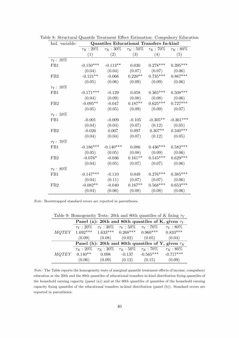
Table 8: Structural Quantile Treatment Effect Estimation: Compulsory Education

Ind. variable: Quantiles Educational Transfers In-kindτK : 20% τK : 30% τK : 50% τK : 70% τK : 80%

(1) (2) (3) (4) (5)

τY : 20%FB1 -0.150*** -0.113** 0.030 0.278*** 0.395***

(0.04) (0.04) (0.07) (0.07) (0.06)FB2 -0.121** -0.066 0.220** 0.735*** 0.867***

(0.05) (0.06) (0.09) (0.09) (0.06)τY : 30%FB1 -0.171*** -0.129 0.058 0.365*** 0.508***

(0.04) (0.09) (0.08) (0.08) (0.06)FB2 -0.095** -0.047 0.187** 0.625*** 0.727***

(0.05) (0.05) (0.09) (0.09) (0.07)τY : 50%FB1 -0.001 -0.009 -0.105 -0.305** -0.361***

(0.04) (0.04) (0.07) (0.12) (0.05)FB2 -0.026 0.007 0.097 0.307** 0.340***

(0.04) (0.04) (0.07) (0.12) (0.05)τY : 70%FB1 -0.186*** -0.140*** 0.086 0.436*** 0.582***

(0.05) (0.05) (0.08) (0.09) (0.06)FB2 -0.076* -0.036 0.161** 0.545*** 0.629***

(0.04) (0.05) (0.07) (0.07) (0.06)τY : 80%FB1 -0.147*** -0.110 0.049 0.276*** 0.385***

(0.04) (0.11) (0.07) (0.07) (0.06)FB2 -0.082** -0.040 0.167** 0.568*** 0.653***

(0.04) (0.06) (0.08) (0.08) (0.06)

Note: Bootstrapped standard errors are reported in parentheses.

Table 9: Homogeneity Tests: 20th and 80th quantiles of K fixing τYPanel (a): 20th and 80th quantiles of K, given τYτY : 20% τY : 30% τY : 50% τY : 70% τY : 80%

MQTEY 1.692*** 1.633*** 0.268*** 0.960*** 0.833***(0.09) (0.08) (0.02) (0.05) (0.04)

Panel (b): 20th and 80th quantiles of Y, given τKτK : 20% τK : 30% τK : 50% τK : 70% τK : 80%

MQTEY 0.140** 0.098 -0.137 -0.565*** -0.717***(0.06) (0.09) (0.12) (0.15) (0.09)

Note: The Table reports the homogeneity tests of marginal quantile treatment effects of income, compulsory

education at the 20th and the 80th quantiles of educational transfers in-kind distribution fixing quantiles of

the household earning capacity (panel (a)) and at the 80th quantiles of quantiles of the household earning

capacity fixing quantiles of the educational transfers in-kind distribution (panel (b)). Standard errors are

reported in parentheses.

40

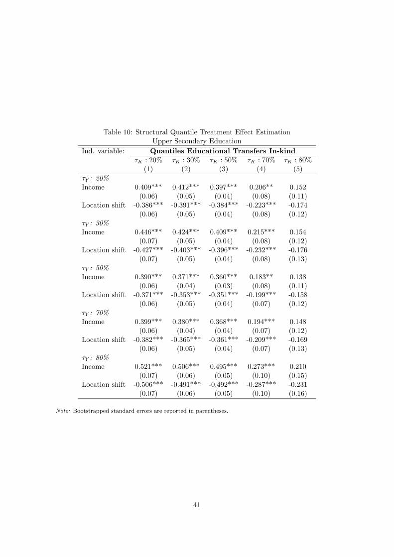
Table 10: Structural Quantile Treatment Effect EstimationUpper Secondary Education

Ind. variable: Quantiles Educational Transfers In-kindτK : 20% τK : 30% τK : 50% τK : 70% τK : 80%

(1) (2) (3) (4) (5)

τY : 20%Income 0.409*** 0.412*** 0.397*** 0.206** 0.152

(0.06) (0.05) (0.04) (0.08) (0.11)Location shift -0.386*** -0.391*** -0.384*** -0.223*** -0.174

(0.06) (0.05) (0.04) (0.08) (0.12)τY : 30%Income 0.446*** 0.424*** 0.409*** 0.215*** 0.154

(0.07) (0.05) (0.04) (0.08) (0.12)Location shift -0.427*** -0.403*** -0.396*** -0.232*** -0.176

(0.07) (0.05) (0.04) (0.08) (0.13)τY : 50%Income 0.390*** 0.371*** 0.360*** 0.183** 0.138

(0.06) (0.04) (0.03) (0.08) (0.11)Location shift -0.371*** -0.353*** -0.351*** -0.199*** -0.158

(0.06) (0.05) (0.04) (0.07) (0.12)τY : 70%Income 0.399*** 0.380*** 0.368*** 0.194*** 0.148

(0.06) (0.04) (0.04) (0.07) (0.12)Location shift -0.382*** -0.365*** -0.361*** -0.209*** -0.169

(0.06) (0.05) (0.04) (0.07) (0.13)τY : 80%Income 0.521*** 0.506*** 0.495*** 0.273*** 0.210

(0.07) (0.06) (0.05) (0.10) (0.15)Location shift -0.506*** -0.491*** -0.492*** -0.287*** -0.231

(0.07) (0.06) (0.05) (0.10) (0.16)

Note: Bootstrapped standard errors are reported in parentheses.

41

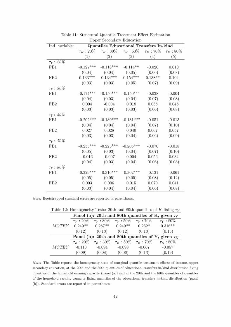
Table 11: Structural Quantile Treatment Effect EstimationUpper Secondary Education

Ind. variable: Quantiles Educational Transfers In-kindτK : 20% τK : 30% τK : 50% τK : 70% τK : 80%

(1) (2) (3) (4) (5)

τY : 20%FB1 -0.127*** -0.118*** -0.114** -0.020 0.010

(0.04) (0.04) (0.05) (0.06) (0.08)FB2 0.133*** 0.134*** 0.154*** 0.138** 0.104

(0.03) (0.03) (0.05) (0.07) (0.09)τY : 30%FB1 -0.174*** -0.156*** -0.150*** -0.038 -0.004

(0.04) (0.03) (0.04) (0.07) (0.08)FB2 0.004 -0.004 0.018 0.058 0.048

(0.03) (0.03) (0.03) (0.06) (0.08)τY : 50%FB1 -0.202*** -0.189*** -0.181*** -0.051 -0.013

(0.04) (0.04) (0.04) (0.07) (0.10)FB2 0.027 0.028 0.040 0.067 0.057

(0.03) (0.03) (0.04) (0.06) (0.09)τY : 70%FB1 -0.233*** -0.223*** -0.205*** -0.070 -0.018

(0.05) (0.03) (0.04) (0.07) (0.10)FB2 -0.016 -0.007 0.004 0.056 0.034

(0.04) (0.03) (0.04) (0.06) (0.08)τY : 80%FB1 -0.329*** -0.316*** -0.302*** -0.131 -0.061

(0.05) (0.05) (0.05) (0.08) (0.12)FB2 0.003 0.006 0.015 0.070 0.041

(0.03) (0.04) (0.04) (0.06) (0.08)

Note: Bootstrapped standard errors are reported in parentheses.

Table 12: Homogeneity Tests: 20th and 80th quantiles of K fixing τYPanel (a): 20th and 80th quantiles of K, given τYτY : 20% τY : 30% τY : 50% τY : 70% τY : 80%

MQTEY 0.249** 0.287** 0.249** 0.252* 0.316**(0.12) (0.13) (0.12) (0.13) (0.15)

Panel (b): 20th and 80th quantiles of Y, given τKτK : 20% τK : 30% τK : 50% τK : 70% τK : 80%

MQTEY -0.113 -0.094 -0.098 -0.067 -0.057(0.09) (0.08) (0.06) (0.13) (0.19)

Note: The Table reports the homogeneity tests of marginal quantile treatment effects of income, upper

secondary education, at the 20th and the 80th quantiles of educational transfers in-kind distribution fixing

quantiles of the household earning capacity (panel (a)) and at the 20th and the 80th quantiles of quantiles

of the household earning capacity fixing quantiles of the educational transfers in-kind distribution (panel

(b)). Standard errors are reported in parentheses.

42

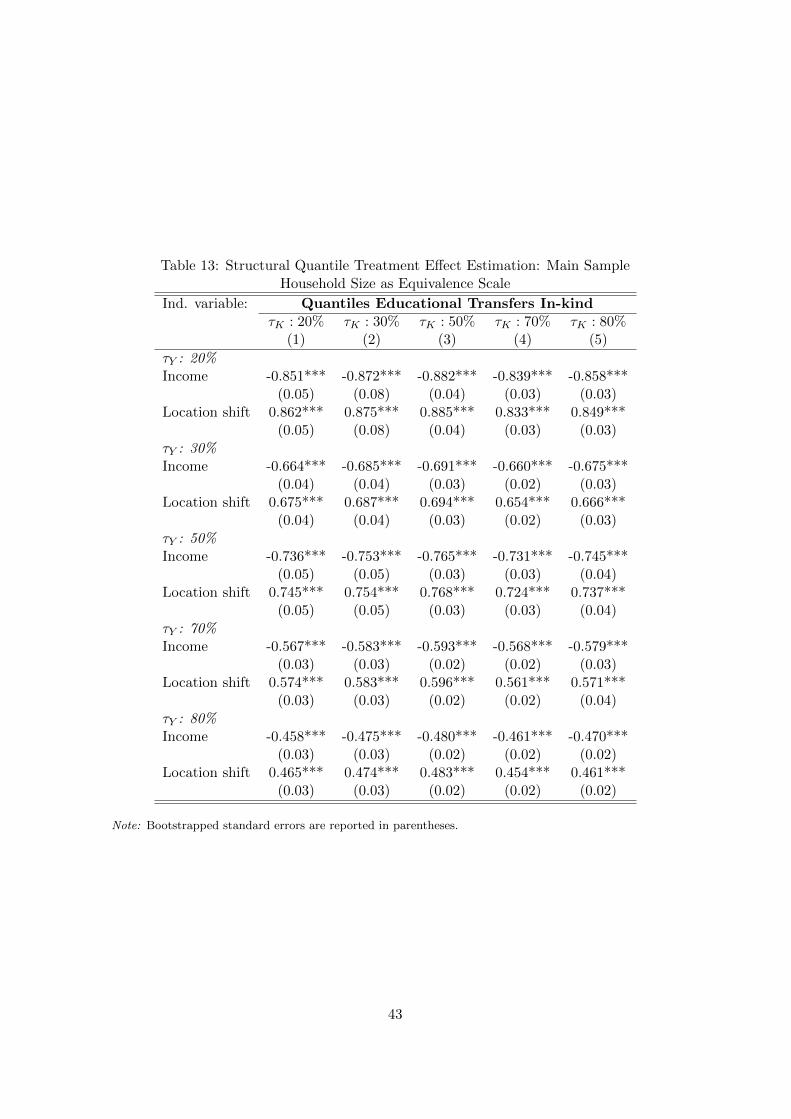
Table 13: Structural Quantile Treatment Effect Estimation: Main SampleHousehold Size as Equivalence Scale

Ind. variable: Quantiles Educational Transfers In-kindτK : 20% τK : 30% τK : 50% τK : 70% τK : 80%

(1) (2) (3) (4) (5)

τY : 20%Income -0.851*** -0.872*** -0.882*** -0.839*** -0.858***

(0.05) (0.08) (0.04) (0.03) (0.03)Location shift 0.862*** 0.875*** 0.885*** 0.833*** 0.849***

(0.05) (0.08) (0.04) (0.03) (0.03)τY : 30%Income -0.664*** -0.685*** -0.691*** -0.660*** -0.675***

(0.04) (0.04) (0.03) (0.02) (0.03)Location shift 0.675*** 0.687*** 0.694*** 0.654*** 0.666***

(0.04) (0.04) (0.03) (0.02) (0.03)τY : 50%Income -0.736*** -0.753*** -0.765*** -0.731*** -0.745***

(0.05) (0.05) (0.03) (0.03) (0.04)Location shift 0.745*** 0.754*** 0.768*** 0.724*** 0.737***

(0.05) (0.05) (0.03) (0.03) (0.04)τY : 70%Income -0.567*** -0.583*** -0.593*** -0.568*** -0.579***

(0.03) (0.03) (0.02) (0.02) (0.03)Location shift 0.574*** 0.583*** 0.596*** 0.561*** 0.571***

(0.03) (0.03) (0.02) (0.02) (0.04)τY : 80%Income -0.458*** -0.475*** -0.480*** -0.461*** -0.470***

(0.03) (0.03) (0.02) (0.02) (0.02)Location shift 0.465*** 0.474*** 0.483*** 0.454*** 0.461***

(0.03) (0.03) (0.02) (0.02) (0.02)

Note: Bootstrapped standard errors are reported in parentheses.

43

Table 14: Structural Quantile Treatment Effect Estimation: Main SampleHousehold Size as Equivalence Scale

Ind. variable: Quantiles Educational Transfers In-kindτK : 20% τK : 30% τK : 50% τK : 70% τK : 80%

(1) (2) (3) (4) (5)

τY : 20%FB1 0.435*** 0.454*** 0.451*** 0.432*** 0.440***

(0.04) (0.04) (0.03) (0.03) (0.03)FB2 0.261*** 0.259*** 0.275*** 0.253*** 0.257***

(0.04) (0.05) (0.03) (0.02) (0.02)τY : 30%FB1 0.424*** 0.445*** 0.441*** 0.423*** 0.431***

(0.04) (0.04) (0.03) (0.03) (0.03)FB2 0.213*** 0.212*** 0.227*** 0.208*** 0.211***

(0.03) (0.03) (0.02) (0.02) (0.02)τY : 50%FB1 0.577*** 0.591*** 0.601*** 0.574*** 0.584***

(0.05) (0.05) (0.03) (0.03) (0.03)FB2 0.263*** 0.270*** 0.277*** 0.256*** 0.259***

(0.04) (0.03) (0.04) (0.03) (0.03)τY : 70%FB1 0.486*** 0.499*** 0.511*** 0.488*** 0.497***

(0.04) (0.04) (0.03) (0.03) (0.04)FB2 0.242*** 0.247*** 0.251*** 0.231*** 0.234***

(0.04) (0.03) (0.03) (0.03) (0.02)τY : 80%FB1 0.376*** 0.389*** 0.398*** 0.380*** 0.388***

(0.04) (0.04) (0.03) (0.03) (0.02)FB2 0.225*** 0.231*** 0.232*** 0.213*** 0.215***

(0.04) (0.03) (0.03) (0.02) (0.02)

Note: Bootstrapped standard errors are reported in parentheses.

44

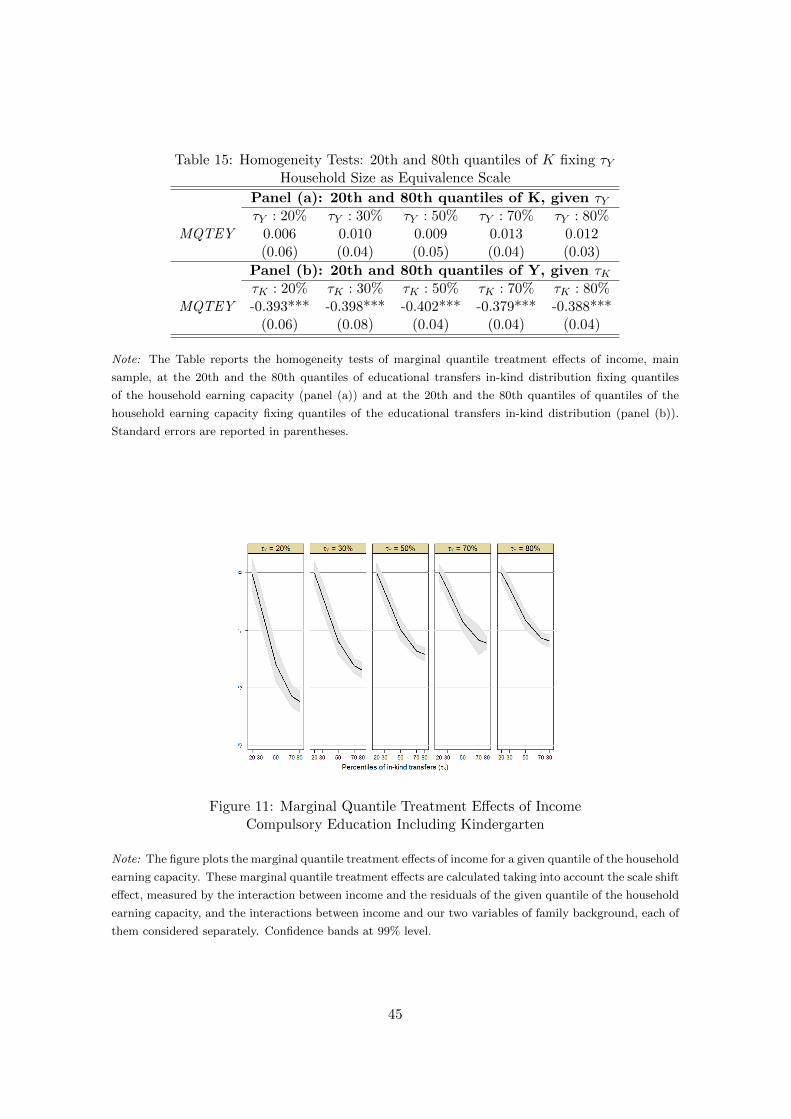
Table 15: Homogeneity Tests: 20th and 80th quantiles of K fixing τYHousehold Size as Equivalence Scale

Panel (a): 20th and 80th quantiles of K, given τYτY : 20% τY : 30% τY : 50% τY : 70% τY : 80%

MQTEY 0.006 0.010 0.009 0.013 0.012(0.06) (0.04) (0.05) (0.04) (0.03)

Panel (b): 20th and 80th quantiles of Y, given τKτK : 20% τK : 30% τK : 50% τK : 70% τK : 80%

MQTEY -0.393*** -0.398*** -0.402*** -0.379*** -0.388***(0.06) (0.08) (0.04) (0.04) (0.04)

Note: The Table reports the homogeneity tests of marginal quantile treatment effects of income, main

sample, at the 20th and the 80th quantiles of educational transfers in-kind distribution fixing quantiles

of the household earning capacity (panel (a)) and at the 20th and the 80th quantiles of quantiles of the

household earning capacity fixing quantiles of the educational transfers in-kind distribution (panel (b)).

Standard errors are reported in parentheses.

Figure 11: Marginal Quantile Treatment Effects of IncomeCompulsory Education Including Kindergarten

Note: The figure plots the marginal quantile treatment effects of income for a given quantile of the household

earning capacity. These marginal quantile treatment effects are calculated taking into account the scale shift

effect, measured by the interaction between income and the residuals of the given quantile of the household

earning capacity, and the interactions between income and our two variables of family background, each of

them considered separately. Confidence bands at 99% level.

45

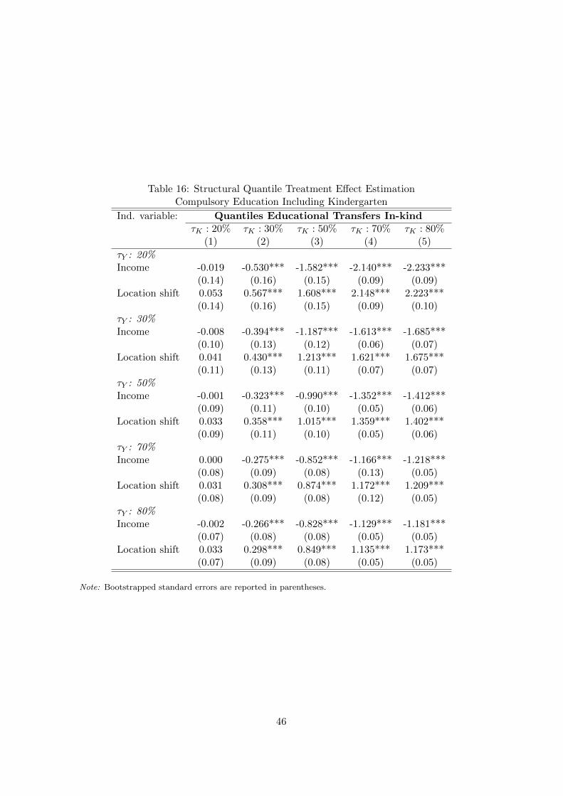
Table 16: Structural Quantile Treatment Effect EstimationCompulsory Education Including Kindergarten

Ind. variable: Quantiles Educational Transfers In-kindτK : 20% τK : 30% τK : 50% τK : 70% τK : 80%

(1) (2) (3) (4) (5)

τY : 20%Income -0.019 -0.530*** -1.582*** -2.140*** -2.233***

(0.14) (0.16) (0.15) (0.09) (0.09)Location shift 0.053 0.567*** 1.608*** 2.148*** 2.223***

(0.14) (0.16) (0.15) (0.09) (0.10)τY : 30%Income -0.008 -0.394*** -1.187*** -1.613*** -1.685***

(0.10) (0.13) (0.12) (0.06) (0.07)Location shift 0.041 0.430*** 1.213*** 1.621*** 1.675***

(0.11) (0.13) (0.11) (0.07) (0.07)τY : 50%Income -0.001 -0.323*** -0.990*** -1.352*** -1.412***

(0.09) (0.11) (0.10) (0.05) (0.06)Location shift 0.033 0.358*** 1.015*** 1.359*** 1.402***

(0.09) (0.11) (0.10) (0.05) (0.06)τY : 70%Income 0.000 -0.275*** -0.852*** -1.166*** -1.218***

(0.08) (0.09) (0.08) (0.13) (0.05)Location shift 0.031 0.308*** 0.874*** 1.172*** 1.209***

(0.08) (0.09) (0.08) (0.12) (0.05)τY : 80%Income -0.002 -0.266*** -0.828*** -1.129*** -1.181***

(0.07) (0.08) (0.08) (0.05) (0.05)Location shift 0.033 0.298*** 0.849*** 1.135*** 1.173***

(0.07) (0.09) (0.08) (0.05) (0.05)

Note: Bootstrapped standard errors are reported in parentheses.

46

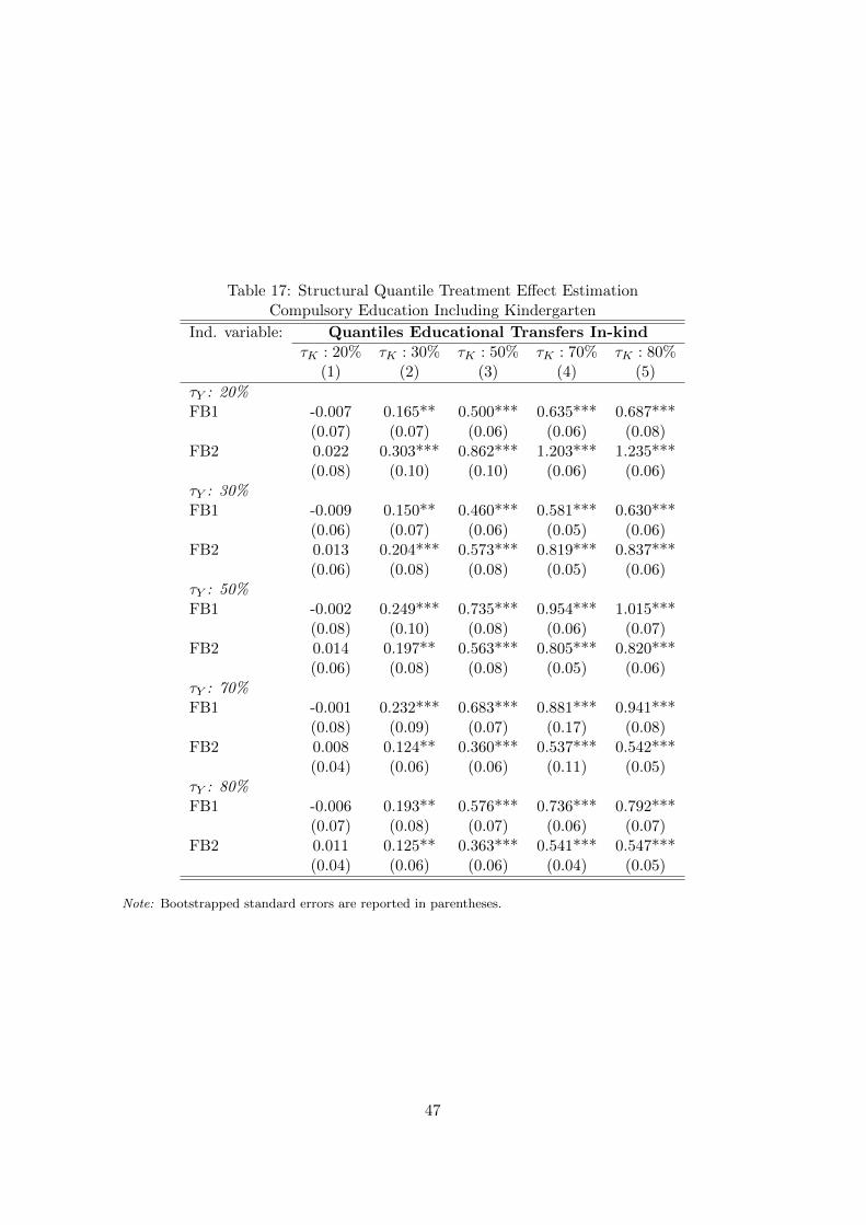
Table 17: Structural Quantile Treatment Effect EstimationCompulsory Education Including Kindergarten

Ind. variable: Quantiles Educational Transfers In-kindτK : 20% τK : 30% τK : 50% τK : 70% τK : 80%

(1) (2) (3) (4) (5)

τY : 20%FB1 -0.007 0.165** 0.500*** 0.635*** 0.687***

(0.07) (0.07) (0.06) (0.06) (0.08)FB2 0.022 0.303*** 0.862*** 1.203*** 1.235***

(0.08) (0.10) (0.10) (0.06) (0.06)τY : 30%FB1 -0.009 0.150** 0.460*** 0.581*** 0.630***

(0.06) (0.07) (0.06) (0.05) (0.06)FB2 0.013 0.204*** 0.573*** 0.819*** 0.837***

(0.06) (0.08) (0.08) (0.05) (0.06)τY : 50%FB1 -0.002 0.249*** 0.735*** 0.954*** 1.015***

(0.08) (0.10) (0.08) (0.06) (0.07)FB2 0.014 0.197** 0.563*** 0.805*** 0.820***

(0.06) (0.08) (0.08) (0.05) (0.06)τY : 70%FB1 -0.001 0.232*** 0.683*** 0.881*** 0.941***

(0.08) (0.09) (0.07) (0.17) (0.08)FB2 0.008 0.124** 0.360*** 0.537*** 0.542***

(0.04) (0.06) (0.06) (0.11) (0.05)τY : 80%FB1 -0.006 0.193** 0.576*** 0.736*** 0.792***

(0.07) (0.08) (0.07) (0.06) (0.07)FB2 0.011 0.125** 0.363*** 0.541*** 0.547***

(0.04) (0.06) (0.06) (0.04) (0.05)

Note: Bootstrapped standard errors are reported in parentheses.

47

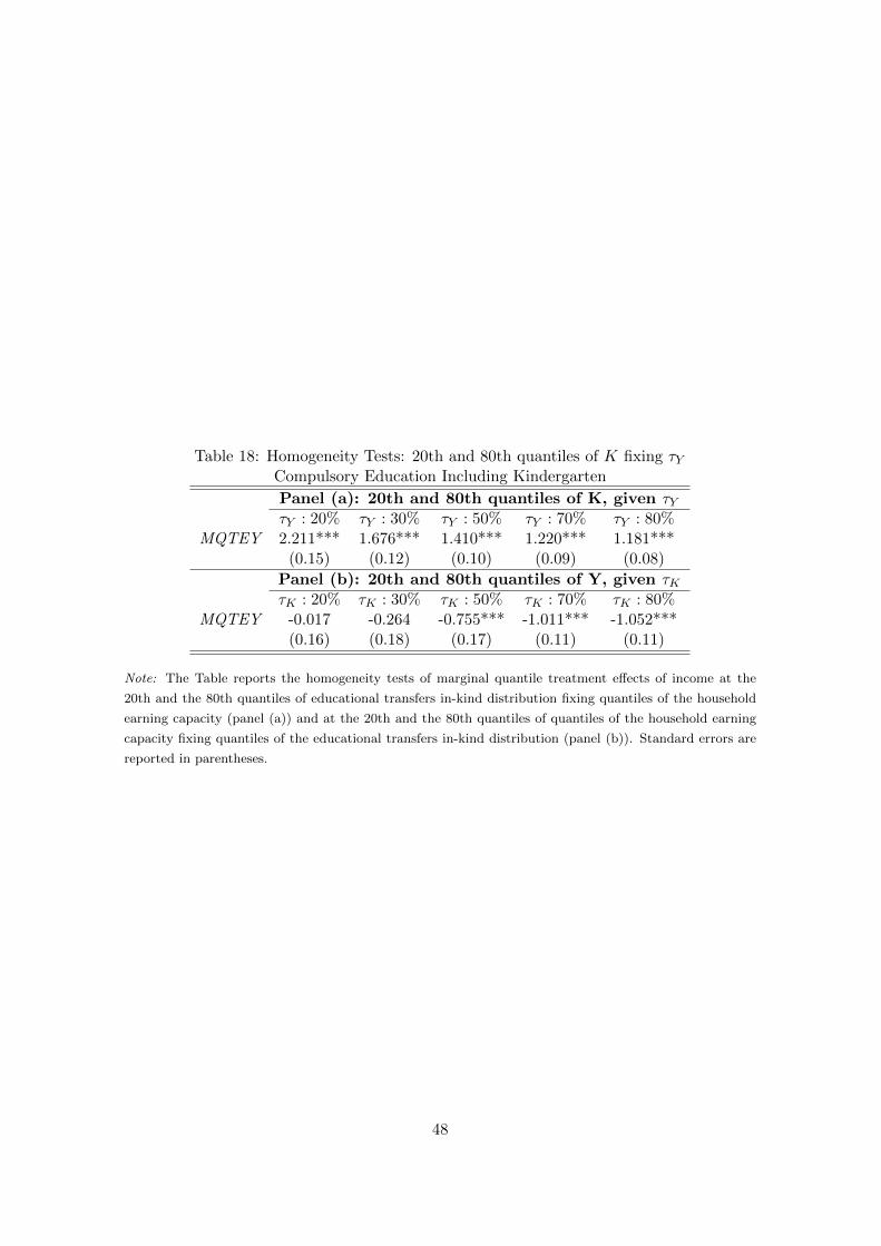
Table 18: Homogeneity Tests: 20th and 80th quantiles of K fixing τYCompulsory Education Including Kindergarten

Panel (a): 20th and 80th quantiles of K, given τYτY : 20% τY : 30% τY : 50% τY : 70% τY : 80%

MQTEY 2.211*** 1.676*** 1.410*** 1.220*** 1.181***(0.15) (0.12) (0.10) (0.09) (0.08)

Panel (b): 20th and 80th quantiles of Y, given τKτK : 20% τK : 30% τK : 50% τK : 70% τK : 80%

MQTEY -0.017 -0.264 -0.755*** -1.011*** -1.052***(0.16) (0.18) (0.17) (0.11) (0.11)

Note: The Table reports the homogeneity tests of marginal quantile treatment effects of income at the

20th and the 80th quantiles of educational transfers in-kind distribution fixing quantiles of the household

earning capacity (panel (a)) and at the 20th and the 80th quantiles of quantiles of the household earning

capacity fixing quantiles of the educational transfers in-kind distribution (panel (b)). Standard errors are

reported in parentheses.

48

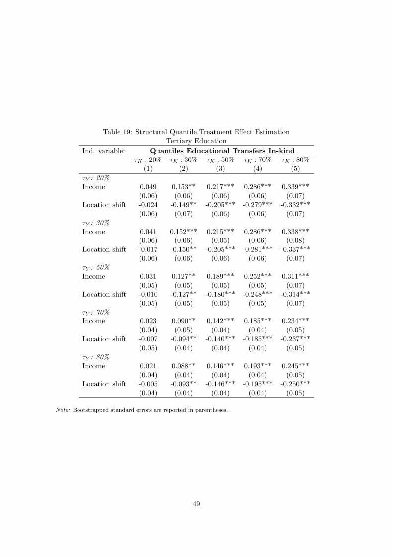
Table 19: Structural Quantile Treatment Effect EstimationTertiary Education

Ind. variable: Quantiles Educational Transfers In-kindτK : 20% τK : 30% τK : 50% τK : 70% τK : 80%

(1) (2) (3) (4) (5)

τY : 20%Income 0.049 0.153** 0.217*** 0.286*** 0.339***

(0.06) (0.06) (0.06) (0.06) (0.07)Location shift -0.024 -0.149** -0.205*** -0.279*** -0.332***

(0.06) (0.07) (0.06) (0.06) (0.07)τY : 30%Income 0.041 0.152*** 0.215*** 0.286*** 0.338***

(0.06) (0.06) (0.05) (0.06) (0.08)Location shift -0.017 -0.150** -0.205*** -0.281*** -0.337***

(0.06) (0.06) (0.06) (0.06) (0.07)τY : 50%Income 0.031 0.127** 0.189*** 0.252*** 0.311***

(0.05) (0.05) (0.05) (0.05) (0.07)Location shift -0.010 -0.127** -0.180*** -0.248*** -0.314***

(0.05) (0.05) (0.05) (0.05) (0.07)τY : 70%Income 0.023 0.090** 0.142*** 0.185*** 0.234***

(0.04) (0.05) (0.04) (0.04) (0.05)Location shift -0.007 -0.094** -0.140*** -0.185*** -0.237***

(0.05) (0.04) (0.04) (0.04) (0.05)τY : 80%Income 0.021 0.088** 0.146*** 0.193*** 0.245***

(0.04) (0.04) (0.04) (0.04) (0.05)Location shift -0.005 -0.093** -0.146*** -0.195*** -0.250***

(0.04) (0.04) (0.04) (0.04) (0.05)

Note: Bootstrapped standard errors are reported in parentheses.

49

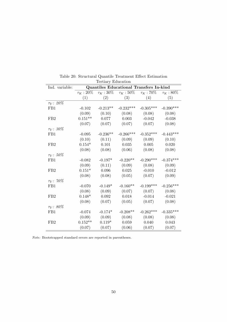
Table 20: Structural Quantile Treatment Effect EstimationTertiary Education

Ind. variable: Quantiles Educational Transfers In-kindτK : 20% τK : 30% τK : 50% τK : 70% τK : 80%

(1) (2) (3) (4) (5)

τY : 20%FB1 -0.102 -0.213** -0.232*** -0.305*** -0.390***

(0.09) (0.10) (0.08) (0.08) (0.08)FB2 0.151** 0.077 0.003 -0.042 -0.038

(0.07) (0.07) (0.07) (0.07) (0.08)τY : 30%FB1 -0.095 -0.236** -0.266*** -0.352*** -0.443***

(0.10) (0.11) (0.09) (0.09) (0.10)FB2 0.154* 0.101 0.035 0.005 0.020

(0.08) (0.08) (0.06) (0.08) (0.08)τY : 50%FB1 -0.082 -0.197* -0.220** -0.290*** -0.374***

(0.09) (0.11) (0.09) (0.08) (0.09)FB2 0.151* 0.096 0.025 -0.010 -0.012

(0.08) (0.08) (0.05) (0.07) (0.09)τY : 70%FB1 -0.070 -0.149* -0.160** -0.199*** -0.256***

(0.08) (0.09) (0.07) (0.07) (0.08)FB2 0.148* 0.092 0.018 -0.014 -0.021

(0.08) (0.07) (0.05) (0.07) (0.08)τY : 80%FB1 -0.074 -0.174* -0.208** -0.262*** -0.335***

(0.09) (0.09) (0.08) (0.08) (0.08)FB2 0.152** 0.119* 0.059 0.040 0.043

(0.07) (0.07) (0.06) (0.07) (0.07)

Note: Bootstrapped standard errors are reported in parentheses.

50

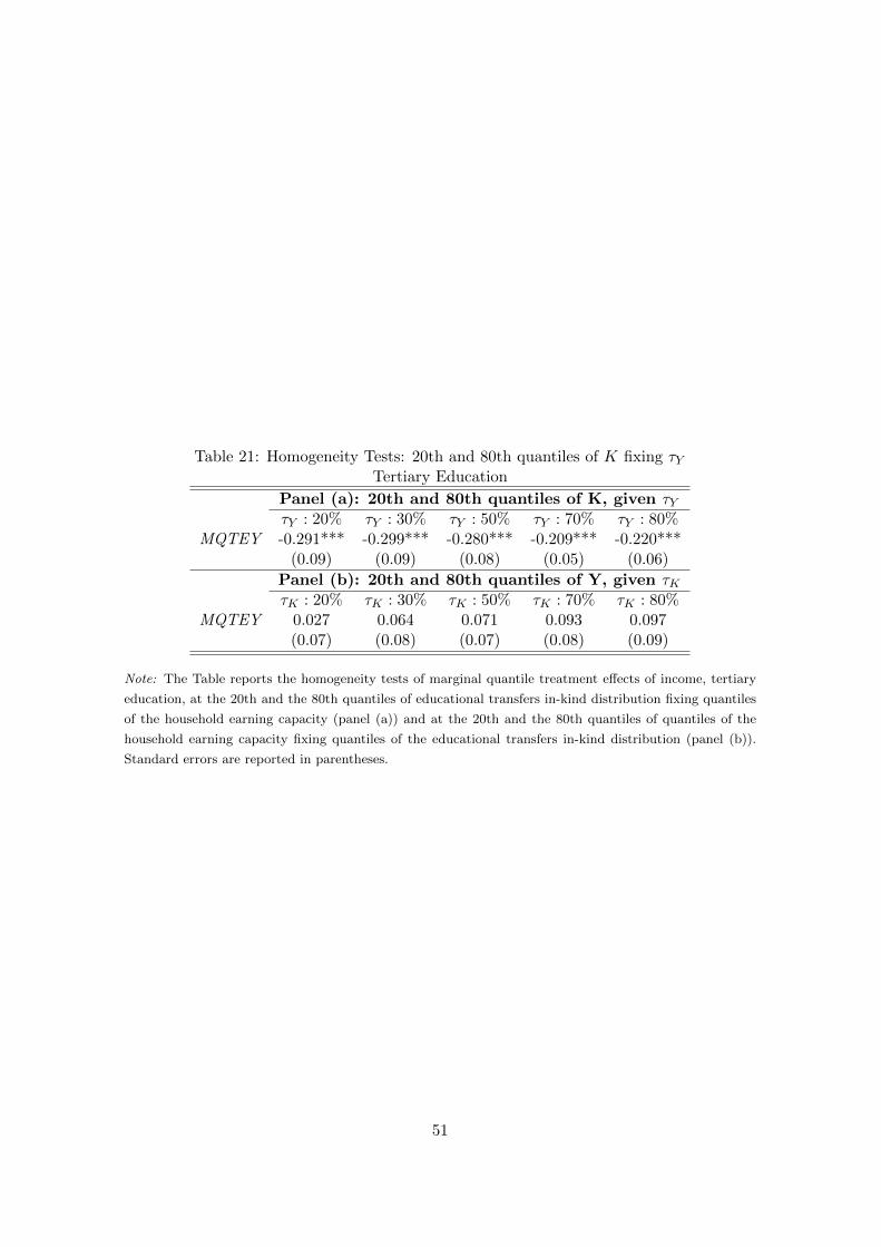
Table 21: Homogeneity Tests: 20th and 80th quantiles of K fixing τYTertiary Education

Panel (a): 20th and 80th quantiles of K, given τYτY : 20% τY : 30% τY : 50% τY : 70% τY : 80%

MQTEY -0.291*** -0.299*** -0.280*** -0.209*** -0.220***(0.09) (0.09) (0.08) (0.05) (0.06)

Panel (b): 20th and 80th quantiles of Y, given τKτK : 20% τK : 30% τK : 50% τK : 70% τK : 80%

MQTEY 0.027 0.064 0.071 0.093 0.097(0.07) (0.08) (0.07) (0.08) (0.09)

Note: The Table reports the homogeneity tests of marginal quantile treatment effects of income, tertiary

education, at the 20th and the 80th quantiles of educational transfers in-kind distribution fixing quantiles

of the household earning capacity (panel (a)) and at the 20th and the 80th quantiles of quantiles of the

household earning capacity fixing quantiles of the educational transfers in-kind distribution (panel (b)).

Standard errors are reported in parentheses.

51