Who Is Easier to Nudge?

John Beshears Harvard University and NBER

James J. Choi

Yale University and NBER

David Laibson Harvard University and NBER

Brigitte C. Madrian

Harvard University and NBER

Sean (Yixiang) Wang NBER

March 18, 2016

Abstract: We study heterogeneity in responsiveness to choice architecture, focusing on the propensity of low-income versus high-income employees to opt out of the default contribution rate in 401(k) retirement savings plans. We develop a statistical model to distinguish between two underlying sources of heterogeneity: low-income employees may be more likely to remain at the default because (i) it is similar to the target contribution rates that they would have selected for themselves anyway or (ii) they are simply slower to opt out of the default, controlling for the target contribution rates that they would select upon opting out. Applying the model to compare below-median-income and above-median-income employees at ten large companies, we estimate that the second source of heterogeneity accounts for two-thirds of the 10 percentage point difference in the probability of remaining at the default after two years of tenure, conditional on having a non-default target contribution rate. We also study two firms that changed the default, and we find that low-income employees are more likely to respond to the change in the default by switching their target contribution rates to correspond with the new default. Keywords: choice architecture, nudge, default, automatic enrollment, savings, 401(k), defined contribution plan, plan design, heterogeneity This research was made possible by grants from the Pershing Square Fund for Research on the Foundations of Human Behavior, the National Institutes of Health (grants P01AG005842 and R01AG021650), and the Social Security Administration (grant RRC08098400). We thank Colin Gray for excellent research assistance. The findings and conclusions expressed are solely those of the authors and do not represent the views of the Pershing Square Fund, the National Institutes of Health, the Social Security Administration, any agency of the Federal Government, or the NBER.

2

Inspired by Thaler and Sunstein’s book Nudge: Improving Decisions about

Health, Wealth, and Happiness (2008) and related work in the fields of behavioral

economics and psychology, academics and policymakers have become increasingly

interested in choice architecture—the design of the environment in which choices are

made—as a tool for influencing individuals’ economic decisions and outcomes. In the

words of David Brooks, a columnist for The New York Times, “We’re entering the age of

what’s been called ‘libertarian paternalism.’ Government doesn’t tell you what to do, but

it gently biases the context so that you find it easier to do things you think are in your

own self-interest” (2013). Indeed, governments around the world have set up “nudge

units,” teams of behavioral scientists who incorporate choice architecture techniques into

the design and execution of policy to improve government functioning.

A large literature has documented that choice architecture techniques can produce

powerful effects.1 However, much of the existing literature has focused on the average

effects of choice architecture techniques, and less attention has been devoted to studying

which types of people are more influenced by nudges and the reasons for such

heterogeneity. This paper studies heterogeneity in responsiveness to choice architecture

in the context of retirement savings plans, focusing on the responses of low-income and

high-income individuals to contribution rate defaults.

The default is the option that is implemented when individuals do not actively

make selections themselves. The default in a retirement savings plan is an important

determinant of outcomes because individuals are likely to accept the default passively

(Madrian and Shea, 2001; Choi et al., 2002 and 2004; Beshears et al., 2008),2 and

previous research has shown that low-income individuals are less likely to opt out of

savings plan defaults than high-income individuals (Madrian and Shea, 2001; Choi et al.,

2004). However, a key challenge that previous research has not addressed is the fact that

a person’s characteristics are often correlated with the person’s preferences over options

within the choice set. In the savings plan context, low-income people tend to prefer lower

contribution rates than high-income people do, perhaps because low-income people 1 For a discussion of the range of choice architecture techniques that have been studied, see Sunstein (2013, 2014). 2 The default also drives outcomes in domains as diverse as e-mail marketing (Johnson, Bellman, and Lohse, 2002), organ donation (Johnson and Goldstein, 2003; Abadie and Gay, 2006), and automobile purchases (Park, Jun, and MacInnis, 2000).

3

expect to experience greater income growth in the future or because the progressivity of

the Social Security system implies that Social Security benefits to low-income people

represent a higher income replacement rate.3 Default contribution rates are also typically

low, often 0%–6% of income, so observed defaults coincide with the preferred

contribution rates of low-income individuals. Carroll et al. (2009) show that individuals

who opt out to contribution rates that are closer to the default tend to opt out more slowly.

Therefore, it is unclear whether low-income individuals are less likely to opt out of

savings plan defaults primarily because defaults implement outcomes close to those that

low-income individuals would have selected for themselves anyway, or primarily

because low-income individuals have a stronger general tendency to accept defaults

passively.

The central contribution of this paper is to distinguish between these two sources

of heterogeneity in responsiveness to savings plan defaults. The distinction is crucial for

policymakers and managers who are responsible for selecting defaults. As noted above,

default contribution rates tend to be modest—in a survey of large companies, Towers

Watson found that the median default among plans that had a non-zero default was 3% of

income (2009). Many observers worry that plans with these defaults will leave employees

with inadequate retirement savings,4 so a natural solution is to increase default

contribution rates beyond the 0%–6% range. However, if low-income employees tend not

to opt out of low default contribution rates primarily because they would have selected

those contribution rates for themselves anyway, defaults higher than 0%–6% would not

necessarily produce more savings, as low-income employees might opt out of the higher

default and implement the lower contribution rates that they prefer. On the other hand, if

low-income employees are simply slower to opt out of defaults, controlling for the

contribution rates that they would select for themselves, it is more likely that higher

defaults would produce additional savings. More generally, policymakers and managers

who are designing retirement savings plans should be cognizant of the groups that are

more impacted by plan defaults.

3 Our analysis is agnostic as to the reason behind the correlation between income and contribution rate preferences. 4 See, for example, (Defined Contribution Institutional Investment Association, 2010).

4

Our empirical approach takes advantage of the dynamic nature of contribution

rate decisions and has the following conceptual underpinnings. When a newly hired

employee joins a firm, the employee draws a target contribution rate from a probability

distribution that is specific to a group of employees with similar characteristics (e.g., the

group of low-income employees).5 An employee’s target contribution rate is defined as

the contribution rate where the employee would eventually end up if given a sufficiently

long time. Upon hire, the employee begins contributing to the retirement savings plan at

the default contribution rate, which may be zero, until the employee actively elects a

different contribution rate. We conceptualize the employee as having an opportunity in

each time period after hire to opt out of the default by incurring an effort cost, which

varies stochastically over time. If the individual’s target rate is equal to the default, the

individual simply remains at the default. Otherwise, we assume that the individual has a

group- and target-rate-specific probability of opting out of the default within the first few

months of hire.6 If the individual with a target rate different from the default does not opt

out within this initial period, we assume that the individual has a constant group- and

target-rate-specific hazard rate for opting out in each subsequent month. Our objective is

to distinguish between the two basic channels that give rise to heterogeneity in

individuals’ likelihood of remaining at the default contribution rate after a given amount

of time has passed since hire. First, there may be heterogeneity in target contribution

rates.7 Second, holding the target contribution rate constant, there may be heterogeneity

in the speed at which individuals opt out of the default to the target rate.

We estimate our statistical model using maximum likelihood methods applied to

monthly contribution rate data from ten large firms, five of which have a default

contribution rate of zero and five of which have a strictly positive default contribution

rate. Our primary model specification compares low-income employees, defined as

5 In our primary model specification, we collapse unpopular contribution rates into bins and treat each bin as a single contribution rate. Our results are similar if we do not use this binning procedure. 6 The exact number of months in this initial period varies across the companies that we study in order to improve the match between the data and our statistical assumptions. 7 The target contribution rate for an individual may or may not be the individual’s ideal contribution rate. If we were to force the individual to actively choose a contribution rate, the individual would select the ideal contribution rate. However, if we instead wait to observe the contribution rate where the individual ends up, the individual may never opt out of the default even though the ideal is different, as the benefit of switching may never exceed the cost. Note that we treat an individual’s target contribution rate as fixed over time, a reasonable assumption given the two-year time horizon that we consider in our empirical analysis.

5

employees with income at or below the sample-wide median, to high-income employees,

defined as employees with income above the sample-wide median. We apply our model

to each company separately, but within each company we estimate the model parameters

for the low-income and high-income groups simultaneously, linking the opt-out

probabilities of the two groups parametrically.8 Our key identifying assumption, which is

consistent with the data, is that individuals from a given group with a given target

contribution rate have a constant monthly hazard rate of opting out to the target rate after

the initial few months employed at the firm. Intuitively, with this assumption, we can use

the month to month trend of opt-outs to a given target contribution rate to estimate the

target rate’s monthly opt-out hazard rate. We can then use the absolute number of opt-

outs and the estimated opt-out hazard rate to infer the size of the target rate population.9

Building on these estimates, we can calculate the opt-out probability for the group and

target rate during the initial few months after hire.

While the estimates from the model vary across the ten firms, as would be

expected given the firms’ different employee populations, the qualitative patterns are

broadly consistent. During the initial few months after hire, the low-income group has

opt-out odds that are smaller than the opt-out odds of the high-income group, holding

constant the target contribution rate, by a factor that ranges from 0.34 to 0.90 across

companies, a ratio that is statistically significantly different from one for nine of the ten

cases. The difference persists beyond this initial period. Again holding the target rate

constant, the low-income group has monthly opt-out odds after the initial period

(conditional on not having opted out previously) that are smaller than those of the high-

8 Specifically, we assume that the low-income employees’ opt-out odds in the initial few months after hire for a given target contribution rate are proportional to the high-income employees’ opt-out odds in the initial few months after hire for the same target contribution rate, and that the ratio between the two is constant across all target contribution rates. We make an analogous proportionality assumption for the monthly opt-out odds (conditional on not having opted out previously) after the initial few months, but we allow the two proportionality factors to differ. We have experimented with relaxing these assumptions and obtained similar results. 9 For example, imagine that we observe employees who opt out to the 5% contribution rate over a span of two months, over which we assume that the probability of opting out in each month is constant. If we observe 20 people opting out in the first month and 16 people opting out in the second month, we can infer that the monthly hazard rate is 20%. We can then combine the hazard rate with the absolute number of employees who opted out to conclude that we started with 100 people who have a target contribution rate of 5%.

6

income sub-group, with the odds ratio ranging from 0.32 to 0.95 across companies. These

estimates are also statistically significantly different from one for nine of the ten cases.

To better interpret the magnitude of these effects, we conduct counterfactual

exercises using the results from our statistical models. For each company, we assume that

the opt-out probabilities of the low-income and high-income groups take the values that

we estimated, but we assume that the target rate distributions for the low-income and

high-income groups are both equal to the average of the estimated target rate distributions

for the two groups. Under these assumptions, we calculate the probability that a low-

income employee who has a target contribution rate different from the default

nonetheless remains at the default two years after hire. We also calculate the same

probability for a high-income employee. We find that the probability for the low-income

employee is greater than the probability for the high-income employee, with the

difference ranging from 3.1 to 20.6 percentage points across companies. The difference is

statistically significant for eight out of ten companies. By construction, the difference is

not due to the divergent target rate distributions of the low-income and high-income

groups. Thus, the evidence indicates that the contribution rates of low-income individuals

are more influenced by defaults than those of high-income individuals, holding fixed the

degree of alignment between individuals’ preferences and the particular options that are

selected as defaults.

Controlling for the target rate distributions in our counterfactual exercises is

important, as the difference in target rate distributions contributes to the overall

difference in the likelihood of remaining at the default in our sample. To document this

point, we again calculate the difference between the low-income employee’s probability

and the high-income employee’s probability of remaining at the default two years after

hire despite having a different target rate, but we change the assumed target rate

distributions to be the estimated low-income distribution and the estimated high-income

distribution, respectively. The difference between the two probabilities is generally larger

compared to the difference when we assume that the target rate distributions are identical.

We also conduct analyses that pool across all ten companies, weighting each

company by the number of employees it contributes to the sample. When we control for

the difference in target rate distributions, we find that low-income employees are 7.1

7

percentage points more likely than high-income employees to remain at the default two

years after hire despite having a different target rate. The difference is 10.2 percentage

points when we do not control for the difference in target rate distributions, indicating

that the difference in target rate distributions accounts for approximately one-third of the

overall effect.

These findings are important considerations for policymakers and managers who

design retirement savings institutions. More broadly, our methodological approach can be

applied to study other domains where choice architecture techniques are used and to

study heterogeneity along dimensions other than income. To explore the application of

our approach to other dimensions of heterogeneity, we use our statistical model to

compare the savings plan contribution rate decisions of younger versus older and male

versus female employees. The difference in the probability of remaining at the default

two years after hire despite having a different target rate is smaller when comparing

younger and older employees relative to when comparing low-income and high-income

employees. However, the decomposition into the two different sources of heterogeneity is

similar. Younger employees are less likely to opt out of the default than older employees,

and approximately one-third of this difference is due to the difference in target rate

distributions. We do not find meaningful differences between male and female employees

in the likelihood of opting out of the default.

As the final step in our analysis, we consider the possibility that contribution rate

defaults differentially influence low-income and high-income employees’ target rate

distributions. In order to pursue this line of inquiry, we study two additional companies,

both of which changed the default contribution rate in their plans, one from 0% to 3%

and the other from 3% to 0%. For each company, we estimate our statistical model

separately for the 0% default regime and for the 3% default regime, and we examine how

the low-income and high-income groups’ estimated target rate distributions shift as the

default changes. The low-income employees exhibit a much larger shift in target rates

than the high-income employees. At one company, the fraction of low-income employees

who have the old default as their target rate decreases by 14 percentage points, while the

fraction who have the new default increases by 21 percentage points. The comparable

numbers for high-income employees at the same company are 8 and 11 percentage

8

points. At the second company, the comparable numbers for low-income employees are

62 and 56 percentage points, and the comparable numbers for high-income employees are

both 39 percentage points. The evidence is consistent with the possibility that low-

income employees exhibit a stronger anchoring effect than high-income employees,

leading low-income employees to adopt the default as their target rate more frequently

(Tversky and Kahneman, 1974; Bernheim, Fradkin, and Popov, 2015), but the data are

also consistent with alternative interpretations.

Our analysis focuses primarily on heterogeneity by income because income is

likely to capture a rich set of factors that influence decision making. Low-income

individuals might exhibit more responsiveness of their target contribution rates to the

default and might be slower to opt out of the default conditional on their target

contribution rates because they have higher cognition or action costs for opting out, a

higher susceptibility to time-inconsistent procrastination, a lack of expertise or

information about financial decisions, or a greater willingness to accept the default

setter’s implicit endorsement of the default option. In addition, a given deviation from the

target contribution rate may have smaller utility consequences for a low-income

individual because of the shape of the individual’s utility function or because of the tax

rates that the individual faces. It is important to note that we do not attempt to disentangle

these correlated factors.

This research is most closely related to the work of Chetty et al. (2014), who use

Danish tax records to study individual responses to government and employer savings

policies. They document that individuals with a higher ratio of wealth to income have a

greater propensity to offset changes in employer-mandated pension contributions by

adjusting savings on other margins, a finding that is similar in spirit to our result that

high-income individuals are in general more likely to opt out of defaults in employer-

sponsored savings plans.

The paper proceeds as follows. In Section I, we explain our statistical model and

empirical methodology. In Section II, we describe the ten retirement savings plans that

we study and the construction of the data set for our primary analysis. We report our

main findings regarding heterogeneity by income group in Section III, the results of

robustness checks in Section IV, and our findings regarding heterogeneity by age group

9

and by gender in Section V. In Section VI, we explore the influence of the default on the

low-income and high-income groups’ target rate distributions. We offer concluding

remarks in Section VII.

I. Methodology

We follow the framework of Carroll et al. (2009) in assuming that each employee

has an ideal 401(k) savings rate s. If an employee is compelled to make an active

decision, he would select this target rate from a menu of all available contribution rates.

Upon first joining the firm, the employee is automatically enrolled at a default savings

rate d.10 In the case that , he faces a flow utility loss in every period until he opts out of

the default rate d and into s. At the beginning of every period, the employee draws a

random transaction cost, and upon learning its realized value, chooses to either opt out of

the default rate, at which point he incurs the realized value of the transaction cost, or

remain at the default rate, at which point he incurs the period’s flow utility loss.

The primary empirical challenge in this setting arises from the problem of

disentangling underlying preferences from observable behavior. If we observe that an

employee has been contributing at the default contribution rate since hire, one of three

possibilities exists. It’s possible that the employee prefers the default contribution rate

over all possible contribution rates – that is, . It is also possible that the employee prefers

a different contribution rate more, but the perceived benefits of switching to that

contribution rate are so small that unless the employee is compelled by active decision,

he will never willingly incur the transaction cost to switch. Finally, it’s possible that the

employee prefers a different contribution rate over the default, and he has yet to

encounter a period in which his transaction costs are low enough to prompt him to switch

to his desired contribution rate; however, he will switch if he is given a sufficiently long

time horizon.

We define an employee as having a target rate c if c is the employee’s most

preferred contribution rate from the menu of all possible contribution rates (c = s), and if

the employee will eventually switch from the default contribution rate to rate c given a

10 Note that this applies whether or not the firm has an explicit automatic enrollment policy, since an opt-in savings plan is equivalent to d = 0.

10

sufficiently long time horizon. If an employee prefers the default contribution rate over

all possible contribution rates, or if he is never willing to incur the transaction cost to

switch from the default rate to his most preferred rate s, we define that employee as

having the default rate as his target rate.

We make two key assumptions to identify the proportion of employees at a firm

who have a non-default target rate. First, we assume that each employee has a constant

target rate upon joining the firm, at least until he switches to that target rate.11 Second, we

assume that after the initial flurry of opt-out activity when employees first join a firm, the

month-to-month probability of opt-out to a given target rate for employees in a similar

income group is constant.12 These two assumptions will allow us to use the observed

distribution of switching over time to each non-default contribution rate to jointly

estimate underlying target rate preferences and switching probabilities for each non-

default target rate.

We divide the new hires at a firm into two groups for comparison along a

dimension of heterogeneity. In this paper, we consider three relevant dimensions: income,

age, and gender. For ease of exposition, we will develop our framework using low- and

high-income employees, but our methods generalize to any arbitrary definition of groups.

We separate the first T months of tenure for each employee into two ranges: the initial

period, , and the later period, . We define a partition of the set of all possible non-default

contribution rates at a firm as . While it is possible to define the partition so that each

element contains only one contribution rate, in which case , etc., we define the setup

generally here as to allow for the possibility of estimating a single set of parameters for a

group of contribution rates. We also define as a singleton that always contains the

default rate, so partitions the set of all possible contribution rates. We let be the

probability that an employee from the high-income group has a target rate in ci, and we

11 This assumption is reasonable given that the longest time horizon that we consider here is two years. 12 A constant hazard rate arises naturally from the Carroll et al. (2009) framework, where individuals independently draw opt-out costs from a common distribution at the beginning each period, and decide to opt out of the default if the perceived benefits to switching exceeds the realized opt-out cost. If there is unobserved heterogeneity within a group that is not captured by differences in target contribution rates, then hazard rates would decline over time instead of remaining constant. We check our constant hazard rate assumption as a robustness check in Section IV, and do not find any evidence that hazard rates change systematically over the first two years of employee tenure.

11

similarly let be the probability that an employee from the low-income group has a target

rate in ci.13

Over the duration of the initial period, an employee with a non-default target rate

in ci from the high-income group has a probability of switching from the default rate d to

his target rate equal to , while an employee with the same target rate from the low-income

group has a probability of switching equal to , where and is the logistic CDF.14 In other

words, the initial period switching odds ratio is constant across target rates.15

During each month in the later period, an employee with a non-default target rate

in ci from the high-income group (who is still at the default contribution rate d) has a

monthly switching hazard rate equal to . That is, conditional on having a non-default

target rate in ci and staying at the default rate until month t in the later period, the

employee has a probability of switching to his target rate during that month equal to . An

analogous employee from the low-income group has a monthly switching hazard rate

equal to .16,17

It follows that an employee in the high-income group switches from the default

rate to his non-default target rate in ci in month t of tenure with probability

13 Notice that we allow for additional heterogeneity between individuals in a specific group (i.e. the low-income group) in two important ways. First, we allow the switching probabilities to vary by the employee’s target rate. Second, we separate the observational period into two separate ranges to allow for differences in the propensity to opt out of the default within each group-target rate cell. Individuals who view the opt-out cost as negligible (i.e. dynamically consistent, pre-committed, or highly financially literature employees) will opt out during the initial period, while individuals prone to delay (i.e. due to procrastination, high learning costs, or generally high transaction costs) will opt out during the later period. 14 For simplicity, we scale the logistic distribution parameters so that 15 There are two practical reasons why we make this assumption. First, our estimation method is most precise when a large number of employees are switching to each contribution rate. By fixing one of the two component parameters across contribution rates, we can still preserve some heterogeneity across contribution rates while also increasing the precision of our parameter of focus. Second, the logistic CDF functional form naturally bounds the overall probability between 0 and 1. It also gives us a familiar interpretation for the parameter as a linearly additive term in log odds, which is analogous to the interpretation of the coefficient of a dummy variable for the low-income group in a logistic regression in which the dependent variable is the probability of switching during the initial period. 16 We make the same assumption for the functional form of θ2 as we did for θ1 for the same reasons specified in the previous footnote. Note, however, that we do allow the odds ratio to vary across periods. We also perform a robustness check that allow both θ1 and θ2 to partially vary by target rate. 17 In theory, it is possible to construct a richer functional form for θ in a way that allows for the simultaneous comparison of three or more groups, or even in a way that incorporates continuous covariates into the functional form. However, in our semi-parametric setup, such an approach would require many ad-hoc assumptions to ensure that we obtain enough degrees of freedom to estimate both the target rate probability and the hazard rate in a stable manner, while offering qualitatively similar results and more difficult to interpret parameters.

12

Meanwhile, an employee in the high-income group stays at the default rate d by the end

of month T with probability

The corresponding probabilities for an employee in the low-income group follows by

substituting for , for , and for .

We observe high (low) income employees who first switch from d to a rate in ci

in their month t of tenure, and high (low) income employees who remain at the default

rate by the end of month T. By taking the logarithm of the product over all individual

likelihood functions, we can reduce the total log-likelihood function to:

To estimate our parameters, we maximize this total log-likelihood function with respect

to and with the constraint that ,, , and . It follows that for each income group, the

probability that an employee has the default contribution rate as the target rate is .

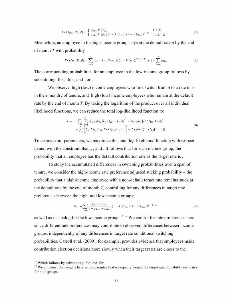
To study the accumulated differences in switching probabilities over a span of

tenure, we consider the high-income rate preference adjusted sticking probability – the

probability that a high-income employee with a non-default target rate remains stuck at

the default rate by the end of month T, controlling for any differences in target rate

preferences between the high- and low-income groups:

as well as its analog for the low-income group. 18,19 We control for rate preferences here

since different rate preferences may contribute to observed differences between income

groups, independently of any differences in target rate conditional switching

probabilities. Carroll et al. (2009), for example, provides evidence that employees make

contribution election decisions more slowly when their target rates are closer to the

18 Which follows by substituting for and for . 19 We construct the weights here as to guarantee that we equally weight the target rate probability estimates for both groups.

13

default rate. Meanwhile, most firms that we study here have a default contribution of 3%

or lower. If low-income employees are more likely to prefer lower contribution rates,

then we would expect to observe a larger proportion of low-income employees at the

default due to differences in target rate preferences alone.

If employees from the low-income group do take longer to switch from the

default rate to their target rates (even after controlling for underlying rate preferences),

we should expect to see evidence of this through a few channels. We may expect that the

initial period switching probability is lower for the low-income group, which is true if

and only if . We may also expect that the later period monthly switching hazard is lower

for the low-income group, which is true if and only if . Finally, we may expect that over

the observation period.

While we explicitly control for heterogeneity in rate preferences between the two

income groups, we recognize that rate preferences are, by themselves, a relevant factor in

influencing opt-out behavior. Therefore, we separately consider the high-income overall

sticking probability – the total probability that a high-income employee with a non-

default target rate remains stuck at the default rate by the end of month T:

as well as its analog for the low-income group.20 Again, if employees from the low-

income group take longer to switch from the default rate to their target rates, we would

expect that . In addition, if the effect of target rate differences stacks on top of any target

rate-conditional switching probability differences, we would expect that .

Wherever possible, we calculate the analytic variance-covariance matrix for our

parameters by taking the inverse of the negative expectation of the likelihood hessian.

Analytic estimates of the standard errors for our test statistics then follow from applying

the multivariate delta method (while allowing for covariance between parameters). In

some cases, our inequality constraints on the parameter space are binding, so the

constrained maximum of our likelihood function is not necessarily the unconstrained

maximum, and the analytic method for calculating the variance-covariance matrix is not

valid. In those cases, we use the bootstrap procedure outlined in Efron and Tibshirani

20 Which follows by substituting for , for , and for .

14

(1993) where we randomly draw with replacement from our original sample 999 times,

estimate all parameters and test statistics for each resample by maximum likelihood, and

use the variance of resampled estimates to conduct inference on the original estimate.21

II. Data

We aim to capture a wide variety of enrollment schemes and firm characteristics

in our paper, so we use a systematic method to select ten candidate firms for analysis. We

begin with the universe of data ranging from 2002 to 2013 from our data provider, Aon

Hewitt, which contain annual snapshots of employee demographics, compensation, and

401(k) eligibility, as well as monthly snapshots of employee contributions for a number

of firms. We separate these firms into two groups: automatic enrollment firms (firms with

default rates > 0%) and standard enrollment firms (firms with default rates = 0%). Some

firms switch enrollment design from standard enrollment to automatic enrollment (or vice

versa), and we split those firms into the two groups according to their timelines under

each enrollment design.

To maintain consistency during the two year observation period for all hires at a

firm (and avoid some potential confounds to observed switching patterns), we exclude

any firms’ hires whose first two years of tenure are affected by automatic escalation, the

offering of a Roth 401(k) plan, any quick enrollment campaigns, any changes in the

default rate or match threshold, or substantial contributions in fractions of a percent or in

dollar amounts. While automatic escalation can be incorporated as a tenure-dependent

default rate, we are unable to observe the month of tenure when an employee opts out of

an automatic escalation plan to stay at his current contribution rate. As a result, we’re

unable to study automatic escalation in this setting without being forced to make much

stronger assumptions on the timing of opt-out choices. We therefore leave the role of

automatic escalation to future research. Meanwhile, the introduction of a Roth 401(k)

21 On rare occasions, we may obtain a resample where the initial or later period hazard parameter for an income group is unidentified or at a corner case. We then exclude that income group-rate combination from the maximum likelihood estimation procedure in that iteration, and assign the affected parameters as missing (in the unidentified case) or to their respective border case values. These special cases do not factor into our estimates for the odds ratios or sticking probabilities, since they have no weight on estimates of the odds ratios and their contribution to the sticking probability is zero in all possible cases. However, we acknowledge these outcomes during the calculation of parameter bootstrap standard errors by including any border case values and assuming the most pessimistic outcomes for the unidentified parameter cases.

15

plan, quick enrollment campaign, or changes to the default or match thresholds would

sufficiently change the incentives for switching contribution rates to the point that our

assumption of a constant month-to-month probability of switching in the later period

would no longer be reasonable for employees whose first two years of tenure overlapped

with these changes. We therefore exclude those firms from our analysis. Finally, we drop

any firms that offer the option of contributing to the 401(k) plan in a flat dollar amount or

in fractions of a percent. This practice is fairly rare, and these non-standard contribution

rates make a firm difficult to compare with the majority of the firms that we study.

After applying the firm-based selection rules, we choose the 5 automatic

enrollment firms and 5 largest standard enrollment firms remaining in the data. Within

each selected firm, we restrict our sample to newly hired, U.S. based employees who are

at least 21 years old at the time of hire and stayed with the firm for at least the full

observational period (which is 24 months long in the main specifications). We do not

necessarily restrict our attention to full time workers as an explicit rule, although we do

eliminate many part time workers indirectly by requiring that all included new hires have

compensation data of at least $5,000 (in 2010 levels) from the year of hire, and become

eligible to contribute in the 401(k) plan within 60 days of hire. 22 We also restrict our

attention to contribution elections to tax-deferred plans, since they are the primary source

of payroll deducted savings in the firms that we study.

Table 1 contains a summary of the main characteristics for the ten firms. By

virtue of our selection criteria, all of the firms that we study are large. We do, however,

observe substantial variation in firm characteristics. These 10 firms operate in 8 different

industries, and their median compensation for new hires range from $27,800 to $86,000.

At the five automatic enrollment firms, default contribution rates range from 2% to 6%.

All ten firms provide matching employer contributions, and the match thresholds vary

from 2% to 6% of contributions. All ten firms have maximum contribution limits that

exceed 10%, and seven firms allow employees to contribute as little as 1% of income to

participate in the 401(k) plan (three exceptions are Firm A, which requires employees to

22 Since the hire dates in our sample range from 2002 to 2010, we adjust compensation data to 2010 levels using the median weekly earnings for full-time workers 16 years and older in the U.S. Bureau of Labor Statistics Current Population Survey

16

contribute at least 3% to participate, and Firms B and D, which requires employees to

contribute at least 2% to participate).

The median compensation across all observed new hires in the final sample is

$62,470. We classify any new hires with income above the overall median income as

high-income employees, and any new hires with income at or below the overall median

income as low-income employees.23 Since we observe employees’ contribution rates as

snapshots at the beginning of each month, we define an employee as having first

switched to a rate in ci in month t of tenure if t full calendar months have elapsed since

the hire date when we first observe the employee contributing at a rate in ci instead of the

default rate d.

In general, we define the initial period to be 2 months long for each firm to cover

any administrative delays in implementing rate elections from the time of hire as well as

to allow for basic eligibility and auto-enrollment delays. However, for three firms, we

define longer initial periods. At Firm B, we do not observe hires’ auto-enrollment status

in the data until the 3rd month of tenure, so we extend the initial period for the firm to 3

months. Meanwhile, Firm A’s employees become eligible for employer matching

contributions after a year of tenure, and we observe a corresponding bump in switching

activity for up to two months after eligibility in the data. We therefore extend Firm A’s

initial period to 14 months to ensure that the initial period for the firm covers the

matching eligibility change and the corresponding increase in switching. Similarly, Firm

I’s employees also become eligible for employer matching contributions after a year of

tenure, but we do not observe any delays in rate elections after the eligibility change. We

therefore extend Firm I’s initial period to 12 months. 24

We determine the partitioning of non-default contribution rates separately for

each firm, based on its plan characteristics. While we would prefer to be able to define all

ci as singletons and estimate parameters separately for each contribution rate, we do not

observe enough new hires switching to unpopular contribution rates (like 1%, 7%, or 9%)

23 We also run robustness checks that split employees into the high- and low-income groups using firm-level median income, income terciles, and income relative to peers with the same gender and age-range. 24 For details about firm plan design and switching patterns, see the data appendix

17

at every firm to precisely estimate parameters in those scenarios.25 So, we use a

systematic rule to determine the partitioning of all possible contribution rates. We always

set aside the default contribution rate as its own rate group. In addition, where possible,

we estimate focal contribution rates like 0%, match thresholds, and 10% by themselves.

We then group together any remaining intervals of contribution rates, with the

assumption that employees who are switching to neighboring, non-focal contribution

rates tend to be similar. In the case that a non-focal contribution rate remains a singleton

after applying this procedure (which occurred with Firm B’s 2% contribution rate and

Firm J’s 1% contribution rate), we group the remaining contribution rate with the nearest

non-default contribution rate.

III. Income Related Differences

Figure 1 presents estimates and confidence intervals for each rate group’s target

rate probabilities. The most popular target rate tends to be the match threshold, which is

consistent with the explanation that the kink in the intertemporal budget curve introduced

by a matching contribution threshold provides a natural accumulation point for

employees with different tastes for savings. A notable exception to this pattern is Firm H,

where an estimated 70.5% of low-income hires and 39.4% of high-income hires have

target rates below the 6% match threshold. This may not be surprising, since Firm H only

matches 25% of employee contributions up to the match threshold, which is the lowest

employer match percentage out of the ten firms that we study.

On the other hand, the default contribution rate appears to be remarkably

unpopular with workers’ underlying contribution rate preferences. At seven out of the

eight firms that set the default contribution rate at a different rate than any match

thresholds, we estimate that at least 85% of new hires in either income group will

eventually choose to incur the transaction cost to opt out of the default rate to a more

attractive contribution rate. Again, the only exception in this group is Firm H, where an

estimated 34.7% of low-income hires and 19.9% of high-income hires have a target rate

equal to the default contribution rate of 0%. Given that our empirical strategy considers

25 We do, however, estimate specifications that consider contribution rates between 0% and 10% individually as robustness checks.

18

employees who are never willing to incur the transaction cost of switching away to their

most desired contribution rate as having the default rate as their target rate, the actual

proportion of employees who would select the default rate under active decision may be

even lower than our default target rate probability estimates. We explore this topic further

in Section VII by estimating the change in target rate probabilities at two firms that

altered their default rates.

The popularity of the match threshold and the relative unpopularity of the default

rate suggest that for at least seven of the ten firms that we study, the adopted default rate

may be a poor choice if firms primarily choose the default rate to minimize opt-outs, a

rule of thumb suggested by Thaler and Sunstein (2003). Alternatively, setting the default

rate to the match threshold may eliminate opt-out costs from 16-60% of employees from

both income groups who have the match threshold as their target rate. Our target rate

results align with separate analysis by Bernheim, Fradkin, and Popov (2015), who show

that when opt-out costs are the main welfare consideration, setting the default rate to the

match threshold tends to maximize employee welfare.26

We also find consistent evidence that low-income employees have lower target

contribution rates than their high-income counterparts. For every firm that we study in

this paper, we find that employees from the low-income group are 3-34 percentage points

more likely to have a target rate that is below the match threshold, while employees from

the high-income group are 3-29 percentage points more likely to have a target rate that is

above the match threshold. The difference is most pronounced at high contribution rates –

we estimate that high-income employees are 16-27 percentage points more likely to have

a target contribution rate of 10% or higher.

Figure 2 presents estimates by income group for the probability that an employee

switches from the default to her target contribution rate during the initial period.

Although our estimates for the initial period switching probabilities are reasonably

precise, we obtain a wide range of estimates across firms and across contribution rates.

Since we vary the length of the initial period for some firms to correspond to different

plan designs, we cannot directly compare the initial period switching probabilities across

26 The author also provides conditions when setting the default rate as 0% may be desirable under some scenarios, but they robustly conclude that setting a default rate that is strictly greater than 0% and less than the match threshold is suboptimal.

19

all ten firms. We can, however, look at the trend of switching probabilities within each

firm. Consistent with Carroll et al. (2009), we find that employees tend to switch more

quickly from the default when their target contribution rates are far from the default.

Figure 3 presents estimates by income group for the probability that an employee

first switches to her target contribution rate during a given month in the later period,

conditional on having remained at the default contribution rate up to that month. Our

estimates for the later period switching hazards are less precise than estimates for the

initial period switching probabilities, but we do observe the same general trend that

employees from both income groups tend to switch more quickly away from the default

rate when their target contribution rates are far from the default.

Our point estimates suggest that at all ten firms, for any target contribution rate,

hires in the low-income group are less likely than hires in the high-income group to

switch from the default rate to their target contribution rate during the initial period. Our

point estimates also suggest that at nine out of ten firms, again for any target contribution

rate, hires in the low-income group are less likely than their high-income peers to switch

from the default rate to their target rate in any given month during the later period. By

construction, the difference in switching probabilities or hazards is constant in log odds

across all contribution rate groups at a firm, so it is unsurprising that the low-income

switching probabilities or hazards differ from their high-income versions in the same

direction for all target contribution rates at each firm. However, we explicitly allow this

difference to vary across periods, so it is surprising that we find such consistent

differences in switching behavior.

We formally test for differences in switching using odds ratios and sticking

probabilities. Column 1 in Table 2 reports estimates for the ratio of low-income to high-

income initial period switching odds, and column 2 reports the same for the later period.

The initial period odds ratio is significantly different from one at the 1% level for nine

out of ten firms. Our estimates for the later period switching odds ratios are less precise,

but significantly different from one at the 1% level for six out of ten firms (one additional

firm is significant at the 5% level, and another firm is significant at the 10% level). To

aggregate any accumulated differences in switching probability, column 3 in Table 3

reports the rate preference adjusted sticking probability difference between the two

20

income groups after the first two years of tenure. When controlling for differences in

target rates between low- and high-income employees, we estimate that low-income

employees with non-default target rates are still 3 to 21 percentage points more likely

than their high-income peers to remain stuck at the default contribution rate.27 The

difference between the low-income group’s and the high-income group’s rate preference

adjusted sticking probability is significantly different from zero at the 1% level for seven

firms, and significant at the 5% level for one additional firm.

We also find some evidence that income-based differences in the distribution of

target rates lead to a greater proportion of low-income employees to be stuck at the

default rate, independently of differences in target-rate specific switching probabilities.

At firms where the default contribution rate is low, employees from the low-income

group should be more likely to be stuck at the default when we allow their target rate

preferences to vary from the firm’s average target rate distribution. Column 6 in Table 3

reports the difference in sticking probabilities when we use each income group’s own

target rate distribution, instead of the firm average target rate distribution used in columns

1-3.28 At all eight firms where the default contribution rate is 3% or lower, moving from

the average target rate distribution to the income group-specific target rate distribution

increased the difference in the estimated proportion of employees stuck at the default

contribution rate. The difference between the low-income group’s and the high-income

group’s overall sticking probabilities is also significantly different from zero at the 1%

level for seven out of the ten firms.

IV. Robustness

We vary a series of inputs to ensure that our results are robust to changes in

specification. These nine robustness checks can be broadly separated into three

categories. Three rate group-related checks change our method for treating unpopular

contribution rates to ensure that our results do not rely on any special grouping of the

rates. Three pay-related checks explore results under alternative definitions of high- and

27 For a formal definition of the rate preference adjusted sticking probability, see equation 4. 28 For a formal definition of the overall sticking probability, see equation 5.

21

low-income employees. Three mechanics-related checks test for the sensitivity of our

results to changes in our underlying identifying assumptions.

Although we use a systematic procedure to partition available contribution rates

into rate groups, we want to verify that our grouping does not generate results in some

special way. So, we apply a series of alternate procedures to determine rate groups. Our

baseline for these checks is the most simple rate grouping possible; we separately

estimate any contribution rate between 0% and 10%, and only group together

contribution rates of 11% or greater. To make sure our results are not solely driven by

switches to high contribution rates, we add an additional specification check in which we

assume that any employee with a target rate of 11% or greater will have switched to that

contribution rate by the end of two years, and we do not estimate switching parameters

for that rate group. Our odds ratio results remain unchanged under these specifications

(see Table A1, columns 2, 3, 6, and 7).

Meanwhile, although our rate preference adjusted and overall sticking probability

differences are qualitatively similar under the new specification, we do see substantial

changes in the magnitude of the point estimates for Firms C, G, H, and I (see Table A2,

columns 2, 3, 6, and 7). The variation in sticking probabilities stems from small sample

issues that are introduced when we separately estimate unpopular contribution rates (like

7% or 9%). Since we only observe a handful of employees ever switching to any

unpopular contribution rate in the later period, we tend to fit the flat, sporadic switching

behavior with very high target rate probabilities and very low hazard rates. This issue

does not affect our odds ratio estimates, which give the most weight to the most populous

contribution rate groups. However, it does strongly affect sticking probabilities, since the

effects of the low hazard rates and high target rate probabilities stack with each other

during the calculation of the sticking probability. To eliminate the issue of unpopular

contribution rates from our individual rate groups specification, we assume that any

employee with an unpopular rate29 as his target rate will have switched within his first

two years of tenure, and we exclude those rates from the maximum likelihood estimation

procedure. Columns 4 and 8 in Tables A1 and A2 report the results from this additional

specification check, and we verify that our results are in line with our main estimates.

29 defined as a rate with an estimated later period hazard rate of 0.01 or less

22

We also use three alternative definitions for income to ensure that our results are

not sensitive to the definition of low- and high-income employees: income terciles,

income relative to age and gender, and income relative to others at the same firm. For

income terciles, we assign an employee into the low-income group if his income is at or

below $48,516, the 1/3 quantile income for the overall sample across firms, and we

assign the hire into the high-income group if his income is at or above $80,395, the 2/3

quantile income. Columns 2 and 6 in Tables A3 and A4 report the results from this

robustness check, and as expected, our results are generally unaffected or stronger when

we use this more strict division rule. To verify that we are not simply picking up proxies

for age or gender effects, we subtract from each employee’s income the corresponding 5-

year age and gender group’s cross firm average income, and then we allocate employees

into low- and high-income groups by the median demeaned income of -$4491. Our

results remain largely unchanged after controlling for age and gender (see columns 3 and

7 in Tables A3 and A4). To address any potential issues around separating employees at

each firm into income groups by the cross-firm median income (for example, due to

industry or firm level differences in benefits that compensates for differences in pay), we

also estimate a version of our model that use each firm’s median income for new hires as

the cutoff rule. While the effect of this change from the main specification varies by firm

(due to differences in firms’ median pay for new hires), our results also remain large

unchanged under this rule (see columns 4 and 8 in Tables A3 and A4).

Finally, we run three checks for the sensitivity of our results to our specification

of the maximum likelihood model. For the five automatic enrollment firms, we estimate

separate odds ratios for contributions rate groups above and below the default rate. A

possible explanation for slower opt-outs from the low-income group is that employees

from the low-income group may have fewer tax advantages from contributing in the tax-

deferred 401(k) plans that we study here, and they therefore face lower costs for delaying

any desired increases to their savings rates. While this is a possible channel, it is unlikely

to be the main factor that explains the slower opt-out rates. For eight out of the ten firms

in our sample that set their default contribution rate below the match threshold, the

employer match on the marginal dollar of contributions above the default rate clearly

outweigh most tax advantages that employees may expect. Nevertheless, given the

23

asymmetry in incentives, we may expect to see differences between employees who opt

out to increase their contribution rates and employees who opt out to decrease their

contribution rates. Columns 2, 3, 7, and 8 in Table A5 and columns 2 and 6 in Table A6

report our results from this exercise. While we lose some precision in our estimates, we

do find evidence that low-income employees opt out more slowly than high-income

employees, regardless of the direction of opt-out.

We may also be concerned that while we select employees for whom key plan

characteristics remain constant during the first two years of tenure, we may pick up

anticipatory effects from upcoming rule changes. If there is a behavioral response to

anticipatory effects, our assumption that the later period switching hazard is constant will

not hold for those hires. We therefore drop the last year of hire in each firm’s sample

(where possible – we only observe a single year of hires at Firm F) to eliminate any

potential anticipatory effects, and our results remain unchanged (see columns 4 and 9 in

Table A5, and columns 3 and 7 in Table A6).30

We run a final test for the sensitivity of our results by relaxing the assumption that

the month to month hazard rate in the later period is constant for each target rate and

income group. We expand our original model by dividing the later period evenly into

two. Employees in the high-income group with a target rate in ci have a monthly

switching hazard of in the first later period , and a monthly switching hazard of in the

second later period . It follows that the overall probability of observing an employee in

the high-income group switching to a contribution rate in ci in month t is then:

Meanwhile, we observe an employee in the high-income group staying at the default rate

d by the end of month T with probability

The corresponding probabilities for an employee in the low-income group follows by

substituting for , for , for , and for . While we lose substantial precision by splitting the

30 Incidentally, this approach also dropped any employees whose later period overlapped with the start of the Great Recession, so we are also able to verify though this robustness check that our results are not driven by asymmetric responses to the Recession.

24

later period in half in this specification, our results remain qualitatively unchanged (see

columns 5, 10, and 11 in Table A5, and columns 4 and 8 in Table A6). We also do not

find any systematic differences in the estimated hazard rates between the first and second

later periods (see Tables A7 and A8).

V. Age and Gender Related Differences

Our methods also extend naturally along dimensions of heterogeneity other than

income. In this section, we examine two other sources of differences between new hires,

age and gender, and explore the extent to which responses to defaults vary along these

two dimensions. Our empirical framework under this section ports directly from Section

I, and we consider the same set of new hires that is studied in Sections II-IV. The primary

change in this section arises from a new division of employees along the relevant

dimension of heterogeneity. Remaining consistent with our income approach, we define

younger employees as employees who are at most 33 years old at the time of hire, the

across firm median age of new hires, and we define older employees as employees who

are at least 34 years old at the time of hire.

Figure 4 presents estimates for the target rate probabilities of younger versus older

employees. Mirroring our results from the main income-related estimates, match

thresholds tend to be the most popular target rates for both younger and older employees,

whereas the default contribution rate is relatively unpopular at the eight firms where the

default rate is not a match threshold. Younger employees are more likely to have a target

rate at or below a match threshold, and they are less likely to have target contribution

rates of 10% or higher.

Column 1 of Table 4 presents estimates for the age related odds ratios in the

initial period, and Column 2 of Table 4 presents the same for the later period. We find

clear evidence that younger employees switch more slowly away from the default rate in

the initial period. The ratio of younger employee switching odds to older employee

switching odds is below one at all ten firms, statistically significant at the 1% level for

eight firms, and statistically significant at the 5% level for one other firm. Meanwhile,

our estimates are less precise in the later period. The switching hazard odds ratios are less

than one at five out of the ten firms (and statistically significant for four out of five

25

firms), approximately one at four firms, and greater than one at one firm (but not

statistically significantly so).

Columns 3 and 6 of Table 5 aggregate switching probabilities into two year

sticking probabilities. Despite the statistically significant differences in switching

probabilities in the initial period, the accumulated differences in sticking probabilities

over the first two years of tenure between younger and older employees are fairly small at

most of the firms that we study. For seven out of ten firms, the difference in rate

preference adjusted sticking probabilities is within 2.5 percentage points, and the

difference in overall sticking probabilities is within 3.2 percentage points. However, we

observe large differences in sticking probabilities between younger and older employees

at three firms, and statistically significant differences at two firms. Moreover, the across

firm average sticking probability differences are both statistically significant from zero at

the 1% level.

Given that income and age are positively correlated, one concern with our age-

related results is that we are simply capturing income effects. To address this, we adjust

each employee’s age by the cross firm average age of employees whose income is in the

same $5000 income range, and separate employees into either the younger or older group

by their relative age compared to other employees with similar incomes. Our odds ratio

results under this check remain qualitatively similar, although the initial period odds

ratios are only statistically significant for three firms and the later period odds ratios are

statistically significant for two firms. However, our sticking probability results actually

become stronger – sticking probability differences are statistically significant for Firm C

as well after controlling for the average age of each income group. Our results on age

related differences match theoretical analysis by Gabaix (2016), who proposes that the

influence of default options in retirement savings plans will diminish as people approach

retirement (and begin paying closer attention to their savings).

Figure 5 presents estimates for the target rate probabilities of female employees

compared to male employees. We find few systematic gender-based differences in the

distribution of target contribution rates across the ten firms in our sample. Two possible

exceptions are Firms G and H, where female employees are more likely than male

employees to target contribution rates that are below the match threshold whereas male

26

employees are more likely than female employees to target contribution rates above the

match threshold.

Column 1 of Table 6 presents the estimates for gender related odds ratios in the

initial period, and Column 2 of Table 6 presents the same for the later period. We find

some evidence that female employees switch more slowly from the default contribution

rate in the initial period. The point estimates for the odds ratios are less than 1 for eight

firms, statistically significant at the 1% level for three firms, and statistically significant

at the 5% level for one other firm. Meanwhile, our estimates are generally imprecise in

the later period and widely distributed around 1; only one point estimate is marginally

significantly different from one at the 10% level.

Columns 3 and 6 of Table 7 compile any differences in switching rates during the

initial and later periods. We find no systematic evidence that female and male employees

have different probabilities of being stuck at the default contribution rate after two years.

The cross firm differences in average sticking probabilities are reasonably precisely

estimated for both sticking probabilities, but they are insignificant both in magnitude and

statistical significance.

VI. Target Rate Probabilities Under Different Default Rates

Our work so far has focused on examining the rate of opt-out from the default rate

to an employee’s target contribution rate, while taking the target contribution rate as

given. However, given that an important channel for plan design is through the choice of

the default contribution rate, a separate, but interesting question is how a change in the

default contribution rate affects the distribution of target rates. There are two separate,

but not mutually exclusive channels through which we expect the choice of default rates

to affect target rates. First, if the default contribution rate has an anchoring effect, then we

would expect that an individual’s ideal contribution rate will shift from the previous

default towards the new default rate.31 In addition, recall that under our framework, two

types of individuals have the default rate as their target contribution rate: people whose

ideal contribution rate is the default contribution rate, and people whose ideal rate is

31 This anchoring effect can have a classical explanation as the rational response to a signal from management about the optimal savings rate, or it can be a psychological bias. For more discussion, see Tversky and Kahneman (1974), Green et al. (1998), or Ariely, Loewenstein, and Prelec (2003).

27

different than the default, but perceive the benefits to switching as sufficiently small that

they will never voluntarily incur the cost to opt out of the default into their ideal rate. If

there is a positive mass of the second type, then we would expect target rates to move

with the default contribution rate, even after holding ideal contribution rates fixed.

To identify the relationship between target rate probabilities and default rates, we

focus on firms in our data that changed their default contribution rates for new hires. Due

to the limited availability of full panel data for many firms in our sample, our criteria for

the selection of firms in this section are more relaxed than the criteria used in the main

specifications. For example, we allow firms to offer a Roth 401(k) plan concurrently with

a tax-deferred plan, although we do drop any hires whose observed tenure overlapped

with the introduction of the Roth plan. Among the set of firms that switched default

contribution rates at some point in our dataset, we identified two firms that have full

contributions panel data for employees hired both before and after the change in the

default.32 Both firms have nonstandard rules that make an employee eligible for matching

contributions anywhere from 12 months to at least 18 months after hire, depending on the

calendar month when the employee joined the firm. A change in the match eligibility

status may violate our assumption that the hazard rate is constant if it takes place during

the later period, and data availability constraints render an 18 month initial period

infeasible to implement. Therefore, we truncate the observational period to the first ten

months of tenure, and define the later period as the 3rd or 4th month of tenure to the 10th

month of tenure.33

Table 8 summarizes the main characteristics of the two firms that we study in this

section. Firm K introduced automatic enrollment for new hires on 6/1/2008 and also 32 One of the firms, Firm K, is missing one month of contribution elections data. We interpolated the elections data accordingly using the employee’s contribution elections immediately before and after the missing month, as well as the average rate of switching for each contribution rate at each month of tenure. For more information, see the data appendix. 33 One may be concerned that this is a misrepresentation of the later period, since we know that the plan in place during the first 10 months of tenure will change in future months. However, notice that as long as the plan design remains constant during the first ten months, then our identifying assumptions still hold. The interpretation of target rates is more complicated with the delayed match eligibility, since an individual who would not save in a 401(k) plan in the absence of a match would only opt out of a 0% default rate in order to save on future opt-out costs when the match becomes relevant. So, that individual would actually have a different target rate if the plan setup in the later period is extended to be infinitely long. However, one can consider the benefit of saving future opt-out costs to be equivalent to a different, less generous matching regime that’s in place throughout the entire later period, and the target rates estimated in this specification are what an employee would choose if that equivalent match regime is in place indefinitely.

28

enrolled any past hires who are not participating in the plan, so the standard enrollment

cohort is truncated to ensure that their observational period does not overlap with any

retroactive automatic enrollment. The firm differs from the firms in our main sample in

that it offers a Roth 401(k) option concurrently alongside the tax-deferred plan for both

cohorts of hires included in the sample. Meanwhile, Firm L removed automatic

enrollment for new hires on 11/1/2003, but did not actively remove any previously auto-

enrolled hires from the savings plan. We are therefore able to include employees hired as

late as 10/31/2003 in the standard enrollment cohort. Employees at this firm only become

eligible to participate in the plan after 60-90 days of tenure, so we include any employees

who become eligible within 90 days (instead of 60 days for other firms), and we define

the initial period for the firm to be 3 months long.

Although sample sizes for both firms are large, our estimates here are less stable

than estimates from our main specifications for two reasons. First, the observation period

here is substantially shorter. Second, we focus on precisely estimating the default target

rate probabilities, which are the most sensitive parameters in our model to small samples

(as discussed in Section IV). As a result, we maximize the sample size in both income

groups by dividing employees in each firm by the firm-specific (but not cohort-specific)

median income, rather than the cross firm median income. Our basic rate grouping

algorithm described in Section II is also insufficient for the limited data available here, so

we group remaining low precision contribution rate estimates with other nearby

estimates. For Firm K, we combine the 7-9% rate group with the 10% rate group.

Meanwhile, for Firm L, we combine the 1-2% rate group with the 4-5% rate group, and

we combine the 10% rate group with the 11%+ rate group.

Figure 6 presents the estimated target rate probability distributions for the two

enrollment cohorts at Firm K, and Table 9 reports the changes to target rate probabilities

after the introduction of automatic enrollment. Low-income employees are 21.0

percentage points more likely to have a target contribution rate of 3% when it is the

default contribution rate, whereas high-income employees are 10.6 percentage points

more likely to do the same. On the other hand, low-income employees are 14.1

percentage points less likely to have a target contribution rate of 0% when is it no longer

the default, and high-income employees are 8.4 percentage points less likely to do the

29

same. Both sets of differences are statistically significant, as well as both differences

between the two income groups’ responses to automatic enrollment. In addition, we find

statistically significant decreases in the 1-2% and 4-5% rate group target rate probability.

Some caution is warranted when interpreting the changes to target rate

preferences at 0% or at higher contribution rates at Firm K, since the introduction of

automatic enrollment overlaps with the onset of the Great Recession. While it’s unlikely

that many employees converged towards 3% as an ideal savings rate due to the

Recession, it is possible that a non-negligible proportion of employees reduced their ideal

contribution rate from high contribution rates to either 0%, the lower bound for 401(k)

contributions, or 6% the match threshold.

Figure 7 presents the estimated target rate probability distributions for the two

enrollment cohorts at Firm L, and Table 10 reports the changes to target rate probabilities

from implementing automatic enrollment. The sample here does not overlap with the

recession, and we verify the main qualitative findings from Firm K. Notably, low-income

employees are 61.7 percentage points more likely to have a target contribution rate of 3%

when it is the default rate, while high-income employees are 39.3 percentage points more

likely to do the same. Meanwhile, nearly symmetrically, low-income employees are 55.8

percentage points less likely to have a target contribution rate of 0% when it is not the

default, and high-income employees are 38.7 percentage points less likely to do the same.

Again, both sets of differences are statistically significant, as well as both differences

between income groups. We also find evidence that setting the default rate at 3% reduces

the probability that employees will choose rates of 1-2% or 4-5% as their target rate,

which matches our findings from Firm K and corroborates the theory that placing a

default rate near, but not at an employee’s ideal rate may induce the employee to shift his

target rate from the ideal rate to the default rate, since the perceived gains to switching

become much smaller.

VII. Conclusion

This paper develops and estimates a statistical model to study the propensity for

low-income and high-income employees to opt out of the default contribution rate in a

savings plan. Low-income employees, relative to high-income employees, are slower to

30

opt out of the default, holding fixed the target contribution rate that would be selected

upon opting out. Also, low-income employees’ target rates are more influenced when the

default changes. Applying the methodology to other dimensions of heterogeneity, we find

that younger employees are slower to opt out of the default than older employees,

controlling for the target contribution rate, but this effect is smaller than the effect for

income. We do not find heterogeneity by gender.

These results have implications for the design of defined contribution retirement

savings plans. Given the powerful influence of the default contribution rate on savings

outcomes, a policymaker or manager who desires to increase savings might set a default

that is higher than the defaults of 0%–6% of income currently observed. Our

methodological approach is not designed to address whether such a default would

improve employees’ welfare, but our evidence suggests that such a default would

increase overall contribution rates because low-income employees would not quickly opt

out to lower contribution rates. Future research should address the optimal design of

savings plans in the face of heterogeneous populations. More generally, heterogeneity in

responsiveness to choice architecture is a topic with important policy implications that

should be examined more extensively.

References:

Abadie, Alberto, and Sebastien Gay. 2006. "The Impact of Presumed Consent Legislation on Cadaveric Organ Donation: A Cross-country Study." Journal of Health Economics 25 (4): 599-620.

Allcott, Hunt. 2011. "Social Norms and Energy Conservation." Journal of Public Economics 95 (9-10): 1082-1095.

Ariely, Dan, George Loewenstein, and Drazen Prelec. 2003. "Coherent Arbitrariness: Stable Demand Curves Without Stable Preferences." Quarterly Journal of Economics 118 (1): 73-106.

Bernheim, B Douglas, Andrey Fradkin, and Igor Popov. 2015. "The Welfare Economics of Default Options in 401(k) Plans." American Economic Review 105 (9): 2798-2837.

Beshears, John, James J Choi, David Laibson, and Brigitte C Madrian. 2013. "Simplification and Saving." Journal of Economics Behavior and Organization 95 (C): 130-145.

Beshears, John, James J Choi, David Laibson, and Brigitte C Madrian. 2008. "The Importance of Default Options for Retirement Savings Outcomes: Evidence from the United States." In Lessons from Pension Reform in the Americas, edited by Stephen J. Kay and Tapen Sinha, 59-87. Oxford: Oxford University Press.

31

Bettinger, Eric P, Bridget Terry Long, Philip Oreopoulos, and Lisa Sanbonmatsu. 2012. "The Role of Simplification and Information in College Decisions: Results from the H&R Block FAFSA Experiment." Quarterly Journal of Economics 127 (3): 1205-1242.

Brooks, David. 2013. "The Nudge Debate." The New York Times, August 9: A19.

Carroll, Gabriel D, James J Choi, David Laibson, Brigitte C Madrian, and Andrew Metrick. 2009. "Optimal Defaults and Active Decisions." Quarterly Journal of Economics 124 (4): 1639-74.

Chetty, Raj, John N Friedman, Soren Leth-Petersen, Torben Nielsen, and Tore Olsen. 2014. "Active vs. Passive Decisions and Crowd-Out in Retirement Savings Accounts: Evidence from Denmark." Quarterly Journal of Economics 129 (3): 1141-1219.

Choi, James J, David Laibson, and Brigitte C Madrian. 2009. "Reducing the Complexity Costs of 401(k) Participation Through Quick Enrollment." In Developments in the Economics of Aging, edited by David A. Wise, 57-82. Chicago: University of Chicago Press.

Choi, James J, David Laibson, Brigitte C Madrian, and Andrew Metrick. 2002. Defined Contribution Pensions: Plan Rules, Participant Choices, and the Path of Least Resistance. Vol. 16, in Tax Policy and the Economy, edited by James Poterba, 67-114. Cambridge, MA: MIT Press.

Choi, James J, David Laibson, Brigitte C Madrian, and Andrew Metrick. 2004. "For Better or For Worse: Default Effects and 401(k) Savings Behavior." In Perspectives on the Economics of Aging, edited by David A. Wise, 81-121. Chicago: University of Chicago Press.

Defined Contribution Institutional Investment Association. 2010. "Raising the Bar: Pumping Up Retirement Savings."

Efron, Bradley, and Robert J. Tibshirani. 1993. An Introduction to the Bootstrap. New York: Chapman & Hall.

Gabaix, Xavier. 2016. "Behavioral Macroeconomics Via Sparse Dynamic Programming." NBER Working Paper No. 21848.

Green, Donald, Karen E. Jacowitz, Daniel Kahneman, and Daniel McFadden. 1998. "Referendum Contingent Valuation, Anchoring, and Willingness to Pay for Public Goods." Resource and Energy Economics 20 (2): 85-116.

Hallsworth, Michael, John A List, Robert D Metcalfe, and Ivo Vlaev. 2014. "The Behavioralist As Tax Collector: Using Natural Field Environments to Enhance Tax Compliance." NBER Working Paper No. 20007.

Johnson, Eric J, and Daniel G Goldstein. 2003. "Do Defaults Save Lives?" Science 302 (5649): 1338-1339.

Johnson, Eric J, Steven Bellman, and Gerald L Lohse. 2002. "Defaults, Framing and Privacy: Why Opting In-Opting Out." Marketing Letters 13 (1): 5-15.

Madrian, Brigitte C, and Dennis F Shea. 2001. "The Power of Suggestion: Inertia in 401(k) Participation and Savings Behavior." Quarterly Journal of Economics 116 (4): 1149-1187.

Pallais, Amanda. 2015. "Small Differences that Matter: Mistakes in Applying to College." Journal of Labor Economics 33 (2): 493-520.

32

Park, C Whan, Sung Youl Jun, and Deborah J MacInnis. 2000. "Choosing What I Want Versus Rejecting What I Do Not Want: An Application of Decision Framing to Product Option Choice Decisions." Journal of Marketing Research 37 (2): 187-202.

Schultz, P Wesley, Jessica M Nolan, Robert B Cialdini, Noah J Goldstein, and Vladas Griskevicius. 2007. "The Constructive, Destructive, and Reconstructive Power of Social Norms." Psychological Science 18 (5): 429-434.

Sunstein, Cass R. 2014. "Nudging: A Very Short Guide." Journal of Consumer Policy 37 (4): 583-588.

Sunstein, Cass R. 2013. "The Storrs Lectures: Behavioral Economics and Paternalism." Yale Law Journal 122 (7): 1826-1899.

Thaler, Richard H, and Cass R Sunstein. 2003. "Libertarian Paternalism." American Economic Review Papers and Proceedings 93 (2): 175-179.

—. 2008. Nudge: Improving Decisions About Health, Wealth, and Happiness. New Haven: Yale University Press.

Towers Watson. 2009. "Managing Defined Contribution Plans in the Current Environment."

Tversky, Amos, and Daniel Kahneman. 1974. "Judgment Under Uncertainty: Heuristics and Biases." Science 185 (4157): 1124-1131.

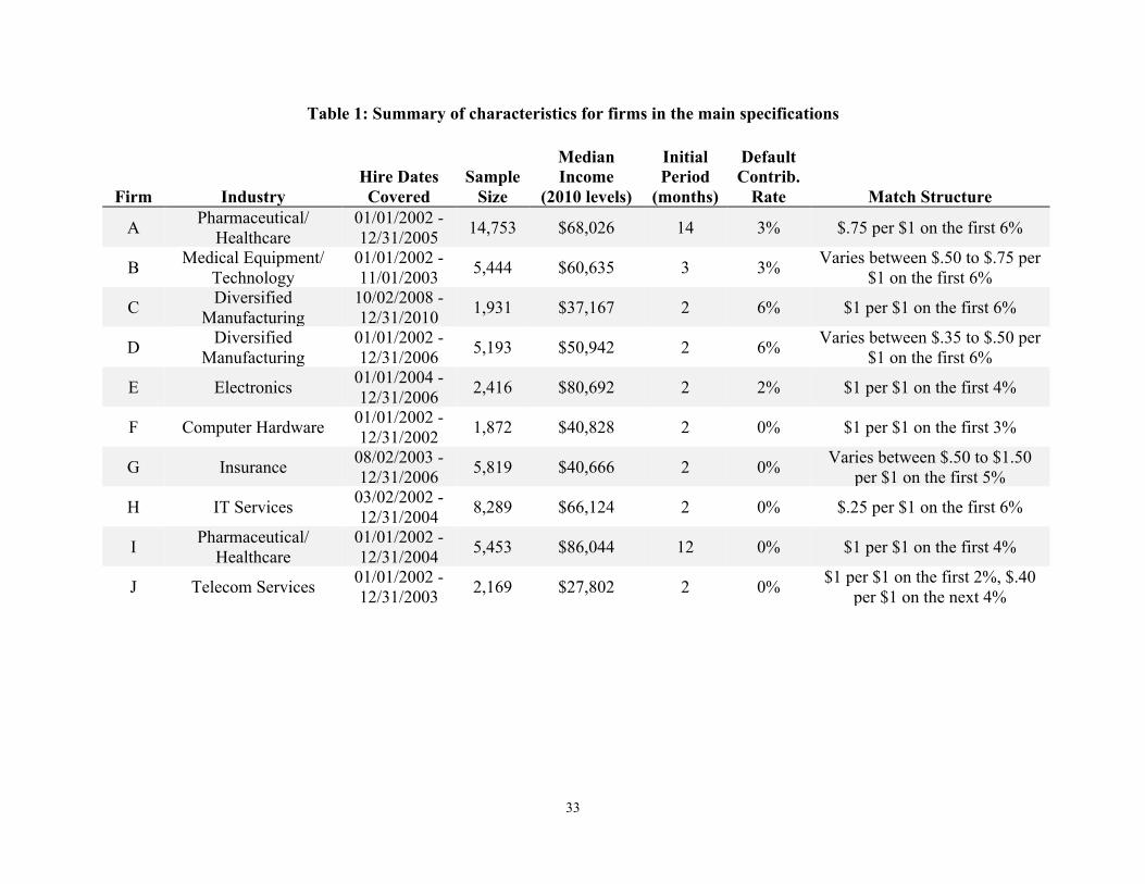
33

Table 1: Summary of characteristics for firms in the main specifications

Firm Industry Hire Dates Covered

Sample Size

Median Income

(2010 levels)

Initial Period

(months)

Default Contrib.

Rate Match Structure

A Pharmaceutical/ Healthcare

01/01/2002 - 12/31/2005 14,753 $68,026 14 3% $.75 per $1 on the first 6%

B Medical Equipment/ Technology

01/01/2002 - 11/01/2003 5,444 $60,635 3 3% Varies between $.50 to $.75 per

$1 on the first 6%

C Diversified Manufacturing

10/02/2008 - 12/31/2010 1,931 $37,167 2 6% $1 per $1 on the first 6%

D Diversified Manufacturing

01/01/2002 - 12/31/2006 5,193 $50,942 2 6% Varies between $.35 to $.50 per

$1 on the first 6%

E Electronics 01/01/2004 - 12/31/2006 2,416 $80,692 2 2% $1 per $1 on the first 4%

F Computer Hardware 01/01/2002 - 12/31/2002 1,872 $40,828 2 0% $1 per $1 on the first 3%

G Insurance 08/02/2003 - 12/31/2006 5,819 $40,666 2 0% Varies between $.50 to $1.50

per $1 on the first 5%

H IT Services 03/02/2002 - 12/31/2004 8,289 $66,124 2 0% $.25 per $1 on the first 6%

I Pharmaceutical/ Healthcare

01/01/2002 - 12/31/2004 5,453 $86,044 12 0% $1 per $1 on the first 4%

J Telecom Services 01/01/2002 - 12/31/2003 2,169 $27,802 2 0% $1 per $1 on the first 2%, $.40

per $1 on the next 4%

34

Table 2: Income specification: initial period and later period switching odds ratios

This table reports the ratio of the odds that a low-income employee will switch from the default contribution rate to his target rate in each period to the odds that a high-income employee will do the same. For the initial period, the switching odds are defined as the probability that the employee switches at any point during the entire period, divided by the probability that the employee does not switch during the period. For the later period, the switching odds are defined as the monthly probability of switching in any given month, conditional on having remained at the default contribution rate up to that month, divided by the probability of staying at the default over the month, conditional on having remained at the default contribution rate up to that month. Standard errors are in parentheses, and any estimates statistically significantly different from one at the 10%, 5% and 1% levels are marked by *, **, and ***, respectively.

Firm Initial Period Later Period A 0.440*** 0.626*** CI (0.021) (0.069)

B 0.476*** 0.936 CI (0.022) (0.118)

C 0.363*** 0.385*** CI (0.027) (0.041)

D 0.519*** 0.954 CI (0.029) (0.136)

E 0.408*** 0.650** CI (0.069) (0.158)

F 0.338*** 0.318*** CI (0.052) (0.076)

G 0.625*** 0.630*** CI (0.042) (0.065)

H 0.512*** 0.534*** CI (0.025) (0.039)

I 0.899 0.689* CI (0.189) (0.175)

J 0.410*** 0.531*** CI (0.031) (0.069)

35

Table 3: Income specification: probability of being stuck at the default contribution rate after 2 years

This table reports the probability that an employee with a non-default target rate will remain at the default rate two years after joining the firm. The first three columns assume that employees from both income groups have the same distribution of target contribution rates, so any differences result purely from differences in the contribution rate-dependent switching probabilities. The last three columns apply each income group’s estimated distribution of target contribution rates to calculate the total probability of being stuck at the default rate. Cross-firm averages are weighted by the total number of observed hires at each firm. Standard errors are in parentheses, and any differences statistically significantly different from zero at the 10%, 5% and 1% levels are marked by *, **, and ***, respectively.

Rate preference adjusted sticking probabilities (Ψ)

Overall sticking probabilities (Ω)

Firm Median or below

Above median

Difference Median or below

Above median

Difference

A 0.056 0.017 0.039*** 0.064 0.015 0.049*** CI (0.014) (0.006) (0.012) (0.017) (0.005) (0.015)

B 0.189 0.134 0.055** 0.226 0.104 0.122 CI (0.101) (0.087) (0.023) (0.124) (0.068) (0.074)

C 0.272 0.073 0.199*** 0.271 0.069 0.202*** CI (0.078) (0.039) (0.064) (0.088) (0.034) (0.077)

D 0.202 0.157 0.045 0.190 0.165 0.025 CI (0.052) (0.048) (0.028) (0.051) (0.051) (0.035)

E 0.120 0.039 0.081*** 0.135 0.033 0.102*** CI (0.017) (0.015) (0.022) (0.019) (0.014) (0.024)

AE Avg 0.125 0.068 0.057*** 0.135 0.062 0.073*** CI (0.021) (0.017) (0.013) (0.024) (0.015) (0.019)

F 0.248 0.042 0.206*** 0.289 0.028 0.261*** CI (0.024) (0.020) (0.034) (0.026) (0.014) (0.029)

G 0.045 0.013 0.032*** 0.054 0.010 0.044*** CI (0.008) (0.005) (0.009) (0.009) (0.004) (0.010)

H 0.207 0.083 0.123*** 0.264 0.059 0.205*** CI (0.034) (0.018) (0.028) (0.044) (0.012) (0.039)

I 0.081 0.050 0.031 0.094 0.042 0.052 CI (0.041) (0.012) (0.041) (0.048) (0.009) (0.048)

J 0.260 0.104 0.156*** 0.325 0.071 0.254*** CI (0.055) (0.047) (0.046) (0.073) (0.033) (0.065)

SE Avg 0.146 0.057 0.089*** 0.180 0.042 0.139*** CI (0.018) (0.010) (0.017) (0.021) (0.007) (0.020)

All Avg 0.134 0.063 0.071*** 0.155 0.053 0.102*** CI (0.014) (0.010) (0.010) (0.017) (0.009) (0.014)

36

Table 4: Age specification: initial period and later period switching odds ratios

This table reports the ratio of the odds that a younger employee will switch from the default contribution rate to his target rate in each period to the odds that an older income employee will do the same. For the initial period, the switching odds are defined as the probability that the employee switches at any point during the entire period, divided by the probability that the employee does not switch during the period. For the later period, the switching odds are defined as the monthly probability of switching in any given month, conditional on having remained at the default contribution rate up to that month, divided by the probability of staying at the default over the month, conditional on having remained at the default contribution rate up to that month. Standard errors are in parentheses, and any estimates statistically significantly different from one at the 10%, 5% and 1% levels are marked by *, **, and ***, respectively.

Firm Initial Period Later Period A 0.834** 1.020 CI (0.072) (0.183)

B 0.739*** 1.066 CI (0.052) (0.146)

C 0.931 0.550*** CI (0.181) (0.089)

D 0.785*** 1.024 CI (0.060) (0.143)

E 0.689*** 1.259 CI (0.111) (0.549)

F 0.723*** 1.079 CI (0.095) (0.292)

G 0.804*** 0.882 CI (0.060) (0.114)

H 0.663*** 0.718*** CI (0.037) (0.062)

I 0.743*** 0.775* CI (0.068) (0.124)

J 0.547*** 0.487*** CI (0.068) (0.067)

37

Table 5: Age specification: probability of being stuck at the default contribution rate after 2 years

This table reports the probability that an employee with a non-default target rate will remain at the default rate two years after joining the firm. The first three columns assume that employees from both income groups have the same distribution of target contribution rates, so any differences result purely from differences in the contribution rate-dependent switching probabilities. The last three columns apply each income group’s estimated distribution of target contribution rates to calculate the total probability of being stuck at the default rate. Cross-firm averages are weighted by the total number of observed hires at each firm. Standard errors are in parentheses, and any differences statistically significantly different from zero at the 10%, 5% and 1% levels are marked by *, **, and ***, respectively.

Rate preference adjusted sticking probabilities (Ψ)

Overall sticking probabilities (Ω)

Firm Younger Older Difference Younger Older Difference A 0.030 0.026 0.004 0.032 0.024 0.008 CI (0.007) (0.007) (0.008) (0.008) (0.007) (0.008)

B 0.181 0.166 0.015 0.186 0.161 0.025 CI (0.122) (0.114) (0.018) (0.124) (0.114) (0.029)

C 0.282 0.169 0.113 0.300 0.152 0.149 CI (0.100) (0.072) (0.070) (0.116) (0.061) (0.097)

D 0.184 0.174 0.010 0.190 0.168 0.021 CI (0.050) (0.049) (0.026) (0.053) (0.048) (0.034)

E 0.078 0.072 0.006 0.083 0.066 0.017 CI (0.036) (0.038) (0.034) (0.036) (0.038) (0.034)

AE Avg 0.105 0.090 0.014 0.109 0.086 0.023* CI (0.020) (0.020) (0.010) (0.021) (0.019) (0.012)

F 0.181 0.163 0.019 0.188 0.156 0.032 CI (0.081) (0.081) (0.044) (0.082) (0.083) (0.055)

G 0.046 0.032 0.014 0.049 0.029 0.021* CI (0.008) (0.008) (0.011) (0.009) (0.007) (0.011)

H 0.177 0.110 0.067*** 0.203 0.092 0.111*** CI (0.031) (0.022) (0.021) (0.036) (0.018) (0.029)

I 0.060 0.034 0.025 0.061 0.034 0.027 CI (0.015) (0.011) (0.016) (0.016) (0.011) (0.017)

J 0.324 0.143 0.181*** 0.347 0.128 0.219*** CI (0.012) (0.028) (0.028) (0.013) (0.027) (0.029)

SE Avg 0.131 0.080 0.051*** 0.144 0.071 0.073*** CI (0.014) (0.011) (0.012) (0.015) (0.010) (0.014)

All Avg 0.116 0.086 0.030*** 0.125 0.079 0.045*** CI (0.013) (0.012) (0.008) (0.014) (0.011) (0.009)

38

Table 6: Gender specification: initial period and later period switching odds ratios

This table reports the ratio of the odds that a female employee will switch from the default contribution rate to her target rate in each period to the odds that a male income employee will do the same. For the initial period, the switching odds are defined as the probability that the employee switches at any point during the entire period, divided by the probability that the employee does not switch during the period. For the later period, the switching odds are defined as the monthly probability of switching in any given month, conditional on having remained at the default contribution rate up to that month, divided by the probability of staying at the default over the month, conditional on having remained at the default contribution rate up to that month. Standard errors are in parentheses, and any estimates statistically significantly different from one at the 10%, 5% and 1% levels are marked by *, **, and ***, respectively.

Firm Initial Period Later Period A 0.806*** 0.839 CI (0.067) (0.121)

B 0.821** 0.840 CI (0.071) (0.100)

C 0.977 1.384 CI (0.190) (0.532)

D 1.161 1.052 CI (0.137) (0.158)

E 0.897 1.446 CI (0.169) (0.458)

F 1.041 1.654 CI (0.175) (0.444)

G 0.657*** 1.013 CI (0.040) (0.152)

H 0.902 0.944 CI (0.062) (0.098)

I 0.663*** 0.777* CI (0.054) (0.124)

J 0.871 1.100 CI (0.121) (0.261)

39

Table 7: Gender specification: probability of being stuck at the default contribution rate after 2 years

This table reports the probability that an employee with a non-default target rate will remain at the default rate two years after joining the firm. The first three columns assume that employees from both income groups have the same distribution of target contribution rates, so any differences result purely from differences in the contribution rate-dependent switching probabilities. The last three columns apply each income group’s estimated distribution of target contribution rates to calculate the total probability of being stuck at the default rate. Cross-firm averages are weighted by the total number of observed hires at each firm. Standard errors are in parentheses, and any differences statistically significantly different from zero at the 10%, 5% and 1% levels are marked by *, **, and ***, respectively.

Rate preference adjusted sticking probabilities (Ψ)

Overall sticking probabilities (Ω)

Firm Female Male Difference Female Male Difference A 0.036 0.025 0.011 0.037 0.025 0.012 CI (0.010) (0.007) (0.008) (0.010) (0.007) (0.009)

B 0.196 0.167 0.029 0.201 0.162 0.039 CI (0.118) (0.112) (0.020) (0.120) (0.111) (0.034)

C 0.128 0.182 -0.055 0.121 0.190 -0.069 CI (0.057) (0.054) (0.053) (0.057) (0.060) (0.064)

D 0.167 0.183 -0.017 0.156 0.194 -0.038 CI (0.050) (0.049) (0.026) (0.048) (0.054) (0.035)

E 0.062 0.082 -0.020 0.062 0.081 -0.019 CI (0.023) (0.015) (0.028) (0.023) (0.015) (0.029)

AE Avg 0.096 0.094 0.003 0.095 0.095 0.000 CI (0.021) (0.019) (0.012) (0.021) (0.020) (0.014)

F 0.131 0.202 -0.071 0.128 0.206 -0.078* CI (0.043) (0.025) (0.044) (0.044) (0.025) (0.047)

G 0.046 0.034 0.012 0.050 0.031 0.019 CI (0.009) (0.008) (0.011) (0.010) (0.008) (0.011)

H 0.137 0.124 0.013 0.145 0.117 0.028 CI (0.026) (0.023) (0.017) (0.028) (0.022) (0.021)

I 0.063 0.033 0.030* 0.063 0.033 0.030* CI (0.016) (0.009) (0.016) (0.016) (0.010) (0.017)

J 0.297 0.309 -0.012 0.317 0.289 0.028 CI (0.077) (0.082) (0.054) (0.085) (0.082) (0.077)

SE Avg 0.112 0.104 0.008 0.117 0.099 0.018 CI (0.012) (0.010) (0.010) (0.013) (0.010) (0.011)

All Avg 0.103 0.098 0.005 0.105 0.097 0.008 CI (0.013) (0.012) (0.008) (0.014) (0.012) (0.010)

40

Table 8: Summary of characteristics for firms that switched default contribution rates

Firm Industry Hire Dates Covered

Sample Size

Median Income

(2010 levels)

Initial Period

(months)

Default Contrib.

Rate Match Structure

K Business Services 01/01/2006 - 06/01/2007 6,851 $67,243 2 0% Varies between $.33 to $1 per

$1 on the first 6%

K Business Services 06/01/2008 - 12/31/2012 18,324 $73,111 2 3% Varies between $.33 to $1 per

$1 on the first 6%

L Healthcare 11/01/2003 - 12/31/2007 18,453 $30,407 3 0% $.50 per $1 on the first 3%

L Healthcare 01/01/2002 - 10/31/2003 7,519 $29,517 3 3% $.50 per $1 on the first 3%

41

Table 9: Effect of automatic enrollment on target contribution rates at Firm K

This table reports the difference between the target rate probability (the probability that an employee has a given target contribution rate) for each rate group when Firm K has a default contribution rate of 3% and the target rate probability when Firm K has a default contribution rate of 0%. The last column reports the difference between the low-income group’s changes and the high-income group’s changes. Standard errors are in parentheses, and any differences statistically significantly different from zero at the 10%, 5% and 1% levels are marked by *, **, and ***, respectively.

Rate Group

Median or below

Above median Difference

0% -0.141*** -0.084*** -0.057** CI (0.028) (0.026) (0.027)

1-2, 4-5% -0.033*** -0.022** -0.011 CI (0.012) (0.011) (0.013)

3% 0.210*** 0.106*** 0.104*** CI (0.020) (0.026) (0.020)

6% 0.031 0.061** -0.030 CI (0.028) (0.030) (0.018)

7-10% -0.042*** -0.016 -0.026** CI (0.007) (0.012) (0.012)

11%+ -0.025*** -0.045*** 0.021** CI (0.005) (0.009) (0.010)

42

Table 10: Effect of automatic enrollment on target contribution rates at Firm L

This table reports the difference between the target rate probability (the probability that an employee has a given target contribution rate) for each rate group when Firm L has a default contribution rate of 3% and the target rate probability when Firm L has a default contribution rate of 0%. The last column reports the difference between the low-income group’s changes and the high-income group’s changes. Standard errors are in parentheses, and any differences statistically significantly different from zero at the 10%, 5% and 1% levels are marked by *, **, and ***, respectively.

Rate Group

Median or below

Above median Difference

0% -0.558*** -0.387*** -0.171*** CI (0.026) (0.026) (0.030)

1-2, 4-5% -0.053*** -0.077*** 0.024 CI (0.019) (0.025) (0.019)

3% 0.617*** 0.393*** 0.224** CI (0.023) (0.129) (0.111)

6-9% 0.000 0.049 -0.049 CI (0.017) (0.113) (0.097)

10%+ -0.005 0.023 -0.027 CI (0.010) (0.058) (0.050)

43

Figure 1: Income based target rate probabilities

For each firm and income group, this figure plots the probability that an employee will have a target contribution rate in each rate group. We denote the default contribution rate for each firm with (d), and any match thresholds with (m). Tick marks on the x axis indicate the end points of each rate group, and line segments on each bar indicate 95% confidence intervals.

44

Figure 2: Income based initial period switching probabilities

For each firm and income group, this figure plots the probability that an employee with a target contribution rate in each rate group will switch from the default rate to the target rate at some point during the initial period. We denote the default contribution rate for each firm with (d), and any match thresholds with (m). Tick marks on the x axis indicate the end points of each rate group, and line segments on each bar indicate 95% confidence intervals.

45

Figure 3: Income based later period switching hazards

For each firm and income group, this figure plots the probability that an employee with a target contribution rate in each rate group will switch from the default rate to the target rate during each month of the later period, conditional on having stayed at the default rate up to that month. We denote the default contribution rate for each firm with (d), and any match thresholds with (m). Tick marks on the x axis indicate the end points of each rate group, and line segments on each bar indicate 95% confidence intervals.

46

Figure 4: Aged based target rate probabilities

For each firm and income group, this figure plots the probability that an employee will have a target contribution rate in each rate group. We denote the default contribution rate for each firm with (d), and any match thresholds with (m). Tick marks on the x axis indicate the end points of each rate group, and line segments on each bar indicate 95% confidence intervals.

47

Figure 5: Gender based target rate probabilities

For each firm and income group, this figure plots the probability that an employee will have a target contribution rate in each rate group. We denote the default contribution rate for each firm with (d), and any match thresholds with (m). Tick marks on the x axis indicate the end points of each rate group, and line segments on each bar indicate 95% confidence intervals.

48

Figure 6: Target rate probabilities for Firm K

This figure plots the estimated target rate probabilities for each rate group under a default contribution rate of 0% (SE) and under a default contribution rate of 3% (AE). At this firm, the match threshold is at 6% for both enrollment regimes. Error bars indicate 95% confidence intervals.

0

0.1

0.2

0.3

0.4

0.5

0.6

0% 1-2,4-5% 3% 6% 7-10% 11%+

Low-incomeGroup

SE AE

0

0.1

0.2

0.3

0.4

0.5

0.6

0% 1-2,4-5% 3% 6% 7-10% 11%+

High-incomeGroup

SE AE

49

Figure 7: Target rate probabilities for Firm L

This figure plots the estimated target rate probabilities for each rate group under a default contribution rate of 0% (SE) and under a default contribution rate of 3% (AE). At this firm, the match threshold is at 3% for both enrollment regimes. Error bars indicate 95% confidence intervals.

0

0.1

0.2

0.3

0.4

0.5

0.6

0.7

0.8

0.9

0% 1-2,4-5% 3% 6-9% 10%+

Low-incomeGroup

SE AE

0

0.1

0.2

0.3

0.4

0.5

0.6

0.7

0.8

0.9

0% 1-2,4-5% 3% 6-9% 10%+

High-incomeGroup

SE AE

50

Table A1: Robustness of odds ratios to various rate groupings

Initial Period Odds Ratios Later Period Odds Ratios

Firm Base Estimates

Individual Target Rates

Individual, Excluding

11%+ Rates

Indiv., Excl.

11%+ & Unpopular

Base Estimates

Individual Target Rates

Individual, Excluding

11%+ Rates

Indiv., Excl.

11%+ & Unpopular

A 0.440*** 0.441*** 0.473*** 0.473*** 0.626*** 0.635** 0.649** 0.649** CI (0.021) (0.068) (0.071) (0.071) (0.069) (0.171) (0.172) (0.172)

B 0.476*** 0.476*** 0.444*** 0.448*** 0.936 0.934 0.906 0.849 CI (0.022) (0.052) (0.052) (0.052) (0.118) (0.181) (0.176) (0.173)

C 0.363*** 0.306*** 0.349*** 0.339*** 0.385*** 0.285*** 0.274*** 0.290*** CI (0.027) (0.073) (0.089) (0.092) (0.041) (0.089) (0.096) (0.108)

D 0.519*** 0.523*** 0.596*** 0.596*** 0.954 0.947 0.948 0.948 CI (0.029) (0.063) (0.085) (0.085) (0.136) (0.179) (0.215) (0.215)

E 0.408*** 0.464*** 0.468*** 0.468*** 0.650** 0.726 0.732 0.732 CI (0.069) (0.079) (0.083) (0.085) (0.158) (0.180) (0.190) (0.197)

F 0.338*** 0.384*** 0.371*** 0.371*** 0.318*** 0.344*** 0.355*** 0.355*** CI (0.052) (0.061) (0.068) (0.068) (0.076) (0.083) (0.101) (0.101)

G 0.625*** 0.606*** 0.596*** 0.596*** 0.630*** 0.566*** 0.538*** 0.538*** CI (0.042) (0.070) (0.073) (0.073) (0.065) (0.122) (0.121) (0.121)

H 0.512*** 0.537*** 0.581*** 0.578*** 0.534*** 0.557*** 0.624*** 0.629*** CI (0.025) (0.050) (0.055) (0.056) (0.039) (0.078) (0.089) (0.100)

I 0.899 0.842 0.742 0.775 0.689* 0.657 0.559** 0.636 CI (0.189) (0.206) (0.184) (0.216) (0.175) (0.259) (0.215) (0.277)

J 0.410*** 0.409*** 0.456*** 0.456*** 0.531*** 0.523*** 0.589** 0.589** CI (0.031) (0.031) (0.100) (0.100) (0.069) (0.067) (0.207) (0.207)

51

Table A2: Robustness of sticking probability differences to various rate groupings

Rate preference adjusted sticking probabilities (Ψ) Overall sticking probabilities (Ω)

Firm Base Estimates

Individual Target Rates

Individual, Excluding

11%+ Rates

Indiv., Excl.

11%+ & Unpopular

Base Estimates

Individual Target Rates

Individual, Excluding

11%+ Rates

Indiv., Excl.

11%+ & Unpopular

A 0.039*** 0.038* 0.033* 0.033* 0.049*** 0.049 0.044 0.044 CI (0.012) (0.021) (0.019) (0.019) (0.015) (0.032) (0.031) (0.031)

B 0.055** 0.052** 0.058*** 0.041 0.122 0.166*** 0.175*** 0.064 CI (0.023) (0.022) (0.022) (0.032) (0.074) (0.043) (0.042) (0.062)

C 0.199*** 0.259*** 0.231*** 0.205*** 0.202*** 0.384*** 0.349*** 0.239** CI (0.064) (0.073) (0.071) (0.075) (0.077) (0.088) (0.095) (0.097)

D 0.045 0.048 0.035 0.035 0.025 0.037 0.032 0.032 CI (0.028) (0.032) (0.034) (0.034) (0.035) (0.087) (0.091) (0.091)

E 0.081*** 0.047** 0.043** 0.061*** 0.102*** 0.071*** 0.071*** 0.099*** CI (0.022) (0.019) (0.019) (0.022) (0.024) (0.020) (0.020) (0.023)

F 0.206*** 0.203*** 0.193*** 0.193*** 0.261*** 0.261*** 0.260*** 0.260*** CI (0.034) (0.027) (0.028) (0.028) (0.029) (0.019) (0.022) (0.022)

G 0.032*** 0.108*** 0.108*** 0.040** 0.044*** 0.174*** 0.176*** 0.051* CI (0.009) (0.031) (0.030) (0.020) (0.010) (0.055) (0.054) (0.030)

H 0.123*** 0.090*** 0.068*** 0.059* 0.205*** 0.344*** 0.325*** 0.088 CI (0.028) (0.024) (0.021) (0.035) (0.039) (0.028) (0.030) (0.064)

I 0.031 0.029 0.047 0.032 0.052 0.130** 0.142** 0.052 CI (0.041) (0.045) (0.046) (0.052) (0.048) (0.065) (0.063) (0.071)

J 0.156*** 0.158*** 0.133** 0.133** 0.254*** 0.257*** 0.239*** 0.239*** CI (0.046) (0.047) (0.056) (0.056) (0.065) (0.068) (0.044) (0.044)

52

Table A3: Robustness of odds ratios to various income group definitions

Initial Period Odds Ratios Later Period Odds Ratios

Firm Base Estimates Terciles Residual

Pay

Firm Median

Pay

Base Estimates Terciles Residual

Pay

Firm Median

Pay A 0.440*** 0.183*** 0.445*** 0.417*** 0.626*** 0.283*** 0.577*** 0.643*** CI (0.021) (0.042) (0.023) (0.018) (0.069) (0.098) (0.063) (0.072)

B 0.476*** 0.256*** 0.479*** 0.454*** 0.936 0.399*** 0.755*** 0.862 CI (0.022) (0.038) (0.023) (0.020) (0.118) (0.099) (0.078) (0.099)

C 0.363*** 0.394*** 0.557*** 0.550*** 0.385*** 0.408*** 0.545*** 0.586*** CI (0.027) (0.046) (0.066) (0.064) (0.041) (0.065) (0.087) (0.102)

D 0.519*** 0.383*** 0.527*** 0.554*** 0.954 1.056 0.922 1.044 CI (0.029) (0.020) (0.029) (0.032) (0.136) (0.220) (0.126) (0.158)

E 0.408*** 0.245*** 0.445*** 0.303*** 0.650** 0.464*** 0.594*** 0.462*** CI (0.069) (0.051) (0.072) (0.056) (0.158) (0.156) (0.142) (0.154)

F 0.338*** 0.244*** 0.295*** 0.274*** 0.318*** 0.260*** 0.332*** 0.325*** CI (0.052) (0.045) (0.049) (0.040) (0.076) (0.076) (0.094) (0.065)

G 0.625*** 0.477*** 0.580*** 0.599*** 0.630*** 0.545*** 0.461*** 0.641*** CI (0.042) (0.033) (0.036) (0.036) (0.065) (0.064) (0.033) (0.065)

H 0.512*** 0.395*** 0.644*** 0.539*** 0.534*** 0.423*** 0.569*** 0.552*** CI (0.025) (0.020) (0.035) (0.026) (0.039) (0.033) (0.039) (0.039)

I 0.899 0.800 0.979 0.682*** 0.689* 0.973 0.761 0.725** CI (0.189) (0.294) (0.211) (0.059) (0.175) (0.596) (0.206) (0.111)

J 0.410*** 0.334*** 0.408*** 0.337*** 0.531*** 0.459*** 0.584*** 0.556*** CI (0.031) (0.076) (0.031) (0.048) (0.069) (0.132) (0.087) (0.097)

53

Table A4: Robustness of sticking probability differences to various income group definitions

Rate preference adjusted sticking probabilities (Ψ) Overall sticking probabilities (Ω)

Firm Base Estimates Terciles Residual

Pay

Firm Median

Pay

Base Estimates Terciles Residual

Pay

Firm Median

Pay A 0.039*** 0.146*** 0.045*** 0.034*** 0.049*** 0.192*** 0.054*** 0.043*** CI (0.012) (0.033) (0.014) (0.010) (0.015) (0.041) (0.017) (0.012)

B 0.055** 0.169*** 0.067*** 0.064*** 0.122 0.312*** 0.138* 0.135* CI (0.023) (0.033) (0.020) (0.022) (0.074) (0.045) (0.071) (0.075)

C 0.199*** 0.186** 0.129** 0.126* 0.202*** 0.194** 0.100 0.100 CI (0.064) (0.081) (0.059) (0.067) (0.077) (0.095) (0.063) (0.076)

D 0.045 0.046 0.050* 0.027 0.025 0.030 0.032 0.006 CI (0.028) (0.034) (0.028) (0.028) (0.035) (0.042) (0.034) (0.035)

E 0.081*** 0.112*** 0.087*** 0.088*** 0.102*** 0.140*** 0.108*** 0.106*** CI (0.022) (0.024) (0.024) (0.019) (0.024) (0.027) (0.026) (0.020)

F 0.206*** 0.240*** 0.210*** 0.240*** 0.261*** 0.296*** 0.260*** 0.293*** CI (0.034) (0.037) (0.038) (0.029) (0.029) (0.029) (0.033) (0.022)

G 0.032*** 0.044*** 0.045*** 0.044*** 0.044*** 0.062*** 0.056*** 0.060*** CI (0.009) (0.011) (0.009) (0.014) (0.010) (0.013) (0.011) (0.016)

H 0.123*** 0.170*** 0.093*** 0.112*** 0.205*** 0.272*** 0.155*** 0.192*** CI (0.028) (0.043) (0.022) (0.025) (0.039) (0.059) (0.030) (0.036)

I 0.031 0.009 0.019 0.033* 0.052 0.026 0.036 0.045** CI (0.041) (0.069) (0.035) (0.018) (0.048) (0.092) (0.040) (0.020)

J 0.156*** 0.174*** 0.139*** 0.199*** 0.254*** 0.318*** 0.246*** 0.257*** CI (0.046) (0.042) (0.046) (0.043) (0.065) (0.033) (0.066) (0.041)

54

Table A5: Robustness of odds ratios to various specification changes

Initial Period Odds Ratios Later Period Odds Ratios

Firm Base Estimates

2 Thetas - Decrease

2 Thetas - Increase

Antici-patory

2 Later Periods

Base Estimates

2 Thetas - Decrease

2 Thetas - Increase

Antici-patory

2 Later Periods 1

2 Later Periods 2

A 0.440*** 0.022*** 0.447*** 0.429*** 0.304*** 0.626*** 0.010*** 0.662* 0.622*** 0.427*** 0.303*** CI (0.021) (0.029) (0.069) (0.021) (0.057) (0.069) (0.015) (0.181) (0.072) (0.110) (0.117)

B 0.476*** 0.505*** 0.470*** 0.337*** 0.500*** 0.936 0.899 0.940 0.515*** 0.940 1.178 CI (0.022) (0.092) (0.091) (0.015) (0.082) (0.118) (0.235) (0.322) (0.046) (0.244) (0.519)

C 0.363*** 0.558*** 0.192*** 0.317*** 0.361*** 0.385*** 0.417*** 0.215*** 0.817 0.344*** 0.555 CI (0.027) (0.167) (0.074) (0.143) (0.132) (0.041) (0.194) (0.105) (0.555) (0.172) (0.444)

D 0.519*** 0.835 0.395*** 0.523*** 0.531*** 0.954 1.022 0.803 1.012 0.974 1.035 CI (0.029) (0.162) (0.057) (0.039) (0.099) (0.136) (0.341) (0.165) (0.204) (0.261) (0.460)

E 0.408*** 0.472** 0.392*** 0.360*** 0.359*** 0.650** 1.055 0.588*** 0.743 0.564*** 0.360*** CI (0.069) (0.225) (0.074) (0.066) (0.069) (0.158) (0.697) (0.156) (0.184) (0.147) (0.188)

F 0.338*** 0.338*** 0.325*** 0.318*** 0.318*** 0.295*** 0.262*** CI (0.052) (0.052) (0.071) (0.076) (0.076) (0.091) (0.180)

G 0.625*** 0.477*** 0.636*** 0.630*** 0.581*** 0.641** 0.715 CI (0.042) (0.034) (0.095) (0.065) (0.077) (0.155) (0.335)

H 0.512*** 0.514*** 0.546*** 0.534*** 0.495*** 0.577** 0.669 CI (0.025) (0.031) (0.137) (0.039) (0.042) (0.185) (0.358)

I 0.899 0.952 1.058 0.689* 0.698 0.807 1.175 CI (0.189) (0.274) (0.382) (0.175) (0.229) (0.410) (0.877)

J 0.410*** 0.572*** 0.562*** 0.531*** 0.724 0.784 1.692 CI (0.031) (0.152) (0.139) (0.069) (0.206) (0.278) (1.184)

55

Table A6: Robustness of sticking probability differences to various specification changes

Rate preference adjusted sticking probabilities (Ψ) Overall sticking probabilities (Ω)

Firm Base Estimates 2 Thetas Antici-

patory 2 Later Periods

Base Estimates 2 Thetas Antici-

patory 2 Later Periods

A 0.039*** 0.101*** 0.037*** 0.104*** 0.049*** 0.137*** 0.046*** 0.131*** CI (0.012) (0.027) (0.012) (0.022) (0.015) (0.036) (0.015) (0.024)

B 0.055** 0.056 0.125*** 0.046 0.122 0.123** 0.217* 0.161*** CI (0.023) (0.037) (0.035) (0.041) (0.074) (0.062) (0.129) (0.061)

C 0.199*** 0.316*** 0.073 0.200 0.202*** 0.340*** 0.188 0.240 CI (0.064) (0.091) (0.117) (0.134) (0.077) (0.111) (0.156) (0.171)

D 0.045 0.075** 0.042 0.028 0.025 0.062 0.013 0.015 CI (0.028) (0.036) (0.043) (0.068) (0.035) (0.044) (0.056) (0.081)

E 0.081*** 0.084*** 0.092*** 0.097*** 0.102*** 0.104*** 0.112*** 0.120*** CI (0.022) (0.023) (0.026) (0.029) (0.024) (0.023) (0.026) (0.028)

F 0.206*** 0.206*** 0.219*** 0.261*** 0.261*** 0.257*** CI (0.034) (0.034) (0.063) (0.029) (0.029) (0.065)

G 0.032*** 0.044*** 0.028 0.044*** 0.058*** 0.038 CI (0.009) (0.013) (0.024) (0.010) (0.015) (0.027)

H 0.123*** 0.137*** 0.100 0.205*** 0.213*** 0.193** CI (0.028) (0.037) (0.093) (0.039) (0.050) (0.095)

I 0.031 0.029 0.002 0.052 0.049 0.025 CI (0.041) (0.054) (0.070) (0.048) (0.062) (0.087)

J 0.156*** 0.079 0.000 0.254*** 0.248*** 0.054 CI (0.046) (0.053) (0.086) (0.065) (0.042) (0.085)

56

Table A7: High-income group hazard rate differences between the 2 later periods

This table reports the difference between the first later period and the second later period high-income hazard rate for each firm and rate group. Match thresholds are highlighted in grey, and unavailable rates are colored in black. We do not estimate hazard rates for any default contribution rates, so those cells are left blank. At Firm B, we group the 2% contribution rate with 0%. Standard errors are in parentheses, and any differences statistically significantly different from zero at the 10%, 5% and 1% levels are marked by *, **, and ***, respectively.

Firm 0% 1% 2% 3% 4% 5% 6% 7% 8% 9% 10% 11%+ A -0.067 #DIV/0! #DIV/0! #DIV/0! 0.007 0.008 -0.132 0.000 0.013 CI (0.125) (0.000) (0.000) (0.000) (0.013) (0.018) (0.138) (0.046) (0.060)

B 0.053 #DIV/0! See Caption

#DIV/0! 0.004 0.014 0.000 0.015 0.037 CI (0.062) (0.000) (0.000) (0.003) (0.015) (0.037) (0.016) (0.114)

C 0.051 0.080 #DIV/0! 0.015 -0.010 -0.007 CI (0.039) (0.060) (0.000) (0.014) (0.091) (0.077)

D 0.002 #DIV/0! 0.009 #DIV/0! -0.016 -0.022 0.012 CI (0.025) (0.000) (0.012) (0.000) (0.014) (0.026) (0.013)

E 0.013 -0.062 -0.037 -0.110 -0.023 CI (0.028) (0.040) (0.037) (0.343) (0.069)

F #DIV/0! -0.066 -0.001 -0.059 -0.052 0.075 CI (0.000) (0.080) (0.031) (0.108) (0.233) (0.108)

G #DIV/0! 0.002 0.007 0.018 0.020 0.042 CI (0.000) (0.027) (0.030) (0.031) (0.107) (0.143)

H #DIV/0! 0.006 0.004 -0.031 0.018 0.028 CI (0.000) (0.007) (0.017) (0.047) (0.014) (0.028)

I #DIV/0! -0.025 0.024** 0.002 -0.007 -0.047 CI (0.000) (0.044) (0.009) (0.025) (0.058) (0.052)

J #DIV/0! 0.015 0.017 0.017 0.022 0.039 0.125 CI (0.000) (0.052) (0.029) (0.062) (0.398) (0.058) (0.174)

57

Table A8: Low-income group hazard rate differences between the 2 later periods

This table reports the difference between the first later period and the second later period low-income hazard rate for each firm and rate group. Match thresholds are highlighted in grey, and unavailable rates are colored in black. We do not estimate hazard rates for any default contribution rates, so those cells are left blank. At Firm B, we group the 2% contribution rate with 0%. Standard errors are in parentheses, and any differences statistically significantly different from zero at the 10%, 5% and 1% levels are marked by *, **, and ***, respectively.

Firm 0% 1% 2% 3% 4% 5% 6% 7% 8% 9% 10% 11%+ A -0.009 #DIV/0! #DIV/0! #DIV/0! 0.010 0.022** -0.032 0.024 0.034 CI (0.042) (0.000) (0.000) (0.000) (0.006) (0.009) (0.064) (0.023) (0.027)

B 0.025 #DIV/0! See Caption

#DIV/0! 0.002 0.000 -0.005 0.004 0.013 CI (0.029) (0.000) (0.000) (0.003) (0.010) (0.024) (0.028) (0.076)

C 0.007 0.020 #DIV/0! 0.000 -0.032 -0.028 CI (0.010) (0.025) (0.000) (0.013) (0.024) (0.039)

D -0.004 #DIV/0! 0.004 #DIV/0! -0.019 -0.028 0.008 CI (0.018) (0.000) (0.013) (0.000) (0.019) (0.023) (0.013)

E 0.018 -0.011 -0.002 -0.020 0.011 CI (0.013) (0.024) (0.017) (0.078) (0.401)

F #DIV/0! -0.018 0.002 -0.015 -0.013 0.031 CI (0.000) (0.057) (0.009) (0.015) (0.054) (0.030)

G #DIV/0! -0.005 -0.002 0.006 0.006 0.021 CI (0.000) (0.015) (0.013) (0.030) (0.043) (0.117)

H #DIV/0! 0.000 -0.006 -0.035 0.003 0.008 CI (0.000) (0.004) (0.026) (0.041) (0.012) (0.015)

I #DIV/0! -0.062 0.000 -0.036 -0.048 0.134 CI (0.000) (0.094) (0.021) (0.048) (0.072) (0.255)

J #DIV/0! -0.020 -0.018 -0.041 -0.115 -0.005 0.056 CI (0.000) (0.013) (0.014) (0.029) (0.112) (0.024) (0.264)

58