Embed Size (px)
Citation preview
Why Brand Manufacturers Should Take Loss LeadingSeriously
Roman Inderst∗ Martin Obradovits†
October 2020
Abstract
Manufacturers frequently resist heavy discounting of their products by retailers,especially when they are used as so-called loss leaders. Since low prices should in-crease demand and manufacturers could simply refuse to fund deep price promotions,such resistance is puzzling at first sight. We explain this phenomenon in a model inwhich price promotions cause shoppers to potentially reassess the relative importanceof quality and price, as they evaluate these attributes relative to a market-wide ref-erence point. With deep discounting, quality can become relatively less important,eroding brand value and the bargaining position of brand manufacturers, hurtingtheir profits and potentially even leading to a delisting of their products. Linkingprice promotions to increased one-stop shopping and more intense retail competition,our theory also contributes to the explanation of the rise of store brands.
∗Johann Wolfgang Goethe University Frankfurt. E-mail: [email protected].†University of Innsbruck. E-mail: [email protected].
1 Introduction
“We take loss leading of our brands very seriously.” This exemplary statement was deliv-
ered by a spokesperson of Foster’s, who justified the company’s blitz action to withdraw
key stock from two Australian supermarket chains after learning of their promotion to
sell Foster’s beer brands below cost.1 It echoes brand manufacturers’ general concerns
about losing margins and brand value when retailers heavily discount their products.2,3
This seems to be the case especially when retailers engage in price wars and promote
branded products to such an extent that they turn into loss leaders. As discounted prices
should however boost demand for the respective manufacturers’ products and as there is
prima facie no reason why manufacturers would need to fund such deep price promotions,
manufacturers’ resistance seems puzzling.
In fact, when consumers exhibit standard preferences, we show that brand manufac-
turers’ fears are unfounded in our model. As retailers’ lower prices expand demand, man-
ufacturers would tend to benefit when their product is chosen as loss leader, rather than
being adversely affected by the retailer’s margin loss. In contrast, our model supports
manufacturers’ resistance against deep discounts when consumers, faced with frequent
price promotions, reassess their relative preferences for price and quality and make such
reassessment dependent on a market-wide reference point. Below we provide various foun-
dations for our formal modelling of such “relative thinking”. As we note there as well, the
1The Sydney Morning Herald, March 23, 2011, “Beer war as Foster’stakes on chains to stop sale of $28 cases”, https://www.smh.com.au/business/
beer-war-as-fosters-takes-on-chains-to-stop-sale-of-28-cases-20110322-1c5cd.html,accessed September 7, 2020.
2Staying with the country of the initial quote, Australia, the following article provides an exam-ple where leading brand manufacturers of bread and milk reported trading losses and the need to cutcost, naming discounted prices at competing retailers as the primary reasons (The Sydney MorningHerald, November 22, 2011, “Heinz hits out at home brands”, https://www.smh.com.au/business/
heinz-hits-out-at-home-brands-20111121-1nr1l.html, accessed September 7, 2020). In the samearticle, as the title suggests, Heinz’ CFO blamed “relentless promotional pressure” at the two nationaldiscounters, Coles and Woolworths, as the main reason for bad financial performance.
3Turning to another country, in a well-known case in 2014, Lidl, one of the largestGerman discounters, stopped selling Coca-Cola, with both sides citing different views aboutthe product’s store price as reason. This was preceded by heavy discounting of Coca-Cola at the discounter (Welt, January 29, 2014, “Coca-Cola kampft sich zuruck in das Lidl-Regal” [“Coca-Cola fights its way back to the Lidl shelf”], https://www.welt.de/wirtschaft/
article124337516/Coca-Cola-kaempft-sich-zurueck-in-das-Lidl-Regal.html, accessed Septem-ber 7, 2020). Given Germany’s notoriously competitive food retailing industry, manufacturersfrequently express concerns about the impact of price wars on their brand value and profits(e.g., Welt, January 29, 2017, “Unilever kritisiert ‘Brandrodung’ im Supermarkt” [“Unilever crit-icizes ‘fire clearing’ in the supermarket”], https://www.welt.de/wirtschaft/article161630067/
Unilever-kritisiert-Brandrodung-im-Supermarkt.html, accessed September 7, 2020).
2
notion that relative preferences over various attributes of an offer depend on some market-
wide reference point has a long-standing tradition in Marketing, Psychology and more
recently Behavioral Economics.4 When consumers exhibit such preferences, retailers’ deep
discounting undermines brand manufacturers’ bargaining power vis-a-vis retailers, leading
to lower profits and possibly even to a delisting of their products, such as in favour of store
brands.
To our knowledge, this paper is the first to analyze the impact of such heavy dis-
counting by retailers on the profits of manufacturers whose brands are discounted in this
way, in contrast to profits of manufacturers in non-promoted categories. Importantly, the
mechanism by which such deep discounting negatively affects manufacturer profit is such
that the manufacturer could not escape these negative implications by adopting retail-
price-maintenance (RPM) strategies (provided that they are not anyhow prohibited by
antitrust laws5). This is so as in our model a retailer’s price-cutting of a particular prod-
uct does not by itself undermine a consumer’s perception of the product’s quality or brand
value.6 Instead, the mechanism depends entirely on the comparison with other offers in
the market, whose lower price (and thereby, the resulting lower reference price) affects the
relative importance of quality and price. To defend the value of their brand and thereby
their bargaining position vis-a-vis retailers, brand manufacturers in a given category would
have to act in concert to prevent that their products are used as loss leaders.7 Such hori-
zontal agreements would clearly fall foul of antitrust laws. Hence, when manufacturers are
rightly concerned that retailers’ loss leading reduces their bargaining position and destroys
brand value, they need to rely on the support of regulation and antitrust laws. In the US
federal law does not restrict below-cost selling, but several states have enacted respective
laws.8 Other countries have stricter rules or specifically forbid below-cost selling in food
4Possibly the most widely known evidence of such preferences relates to an experiment conducted byTversky and Kahnemann (1981). They document that 68% of subjects were willing to drive 20 minutes tosave $5 on the purchase of a calculator when the price was $15, but less than half of this fraction (29%)were willing to do so in order to save again $5 when the price was instead $125.
5RPM is severely restricted in the European Union, where some countries even treat it similarly toanticompetitive practices prohibited per se. Since the 2007 Leegin-decision of the US Supreme court,which clearly ruled against a per-se prohibition of RPM, in the US matters are less clear-cut – also assome states, like California under the Cartwright-Act, still seem to practice such a prohibition.
6Indeed, such a mechanism would seem more reasonable with luxury products, where a high price mayitself be a vital trait of the product (e.g., as it communicates to others the owner’s income and wealth oras it ensures that there is only a small, selective group of such owners).
7As unilateral strategies have no effect, this also applies to the threat of terminating dealers when theydo not adhere to a certain price. At least in the US, under the so-called “Colgate exception”, such apractice would typically not be regarded as unlawful.
8In California, for instance, Section 17044 in the Business and Professions Code states that “[i]t is
3
retailing. Even when there is no outright ban or when this is not rigorously enforced, man-
ufacturers may be able to constrain retailers by raising the awareness of policymakers or
the public.9
In our model, the depth of discounts offered in the promoted category is tightly linked
to the extent of consumer one-stop shopping, that is, the size of consumers’ baskets at
individual shopping trips. For the retailer, this warrants deep discounts on selected items
to compete for consumers’ overall basket. Our mechanism may thus shed new light on some
general trends that shaped retailing over the last decades, particularly in the food sector.
In our model, retailers ultimately replace branded high-quality products with potentially
lower-quality store brands (private labels). Even when this is (still) not the case, one-stop
shopping shifts bargaining power towards retailers and away from brand manufacturers,
as brand value becomes less of an advantage, at least in the promoted category. Precisely,
when the price level in the promoted category decreases due to an increase in one-stop
shopping, low price, rather than superior brand quality, becomes relatively more important
in the eyes of consumers. This may have contributed to the widely observed growth of
private labels.10 Also, again following the main thrust of our model and argument, an
increase in competition for promoted products reduces the bargaining power of brand
manufacturers, which can thus no longer bank on their superior quality or investment
in brand value. In our concluding remarks, we argue how this should have far-reaching
implications for brand manufacturers’ product positioning and investment strategies.
Another insight of our model is that brand manufacturers, particularly those of promotion-
intense, loss-leading products, should be aware of increasing retail competition. This could
be triggered by the entry of hard discounters or, potentially, also by the rise of alternative
shopping formats, such as online retailing – even more so if this forces retailers to compete
more aggressively on few, particularly visible products.
We set up an analytically tractable model that combines retail price promotions,
manufacturer-retailer negotiations and manufacturer vertical differentiation – solved both
unlawful for any person engaged in business within this State to sell or use any article or product as a‘loss leader’ as defined in Section 17030 of this chapter.”
9The latter applies to Germany since the 2017 reform of the antitrust law. Other European countriesthat have restrictions on below-cost pricing are Belgium, France and Ireland.
10There is by now a large literature documenting and analyzing the spread of store brands. For an earlysurvey see, e.g., Berges-Sennou et al. (2004). Various rationales have been proposed for why retailersintroduce store brands, e.g., so as to exert downwards pricing pressure on national brands (Mills (1995);cf. Chitagunta et al. (2002) for an empirical analysis). In our model, instead, retailers are only reactiveto external forces (e.g., the increase in one-stop shopping). As, in line with the literature, shoppers in ourmodel exhibit the same preferences, at present our model can not be immediately extended to the casewhere in a given category store brands and national brands are simultaneously offered by a given retailer.
4
with standard consumer preferences and preferences exhibiting “relative thinking”. This
framework, which remains tractable even under such modified preferences, may prove use-
ful also for other research questions. Precisely, our model combines the following four key
elements. First, to capture frequent price promotions, we employ a “model of sales”, as
in Varian (1980) or Narasimhan (1988). Second, due to limitations either in consumer
attention or advertising space, such promotions take place only in one category, following
Lal and Matutes (1994).11 We can compare implications for this loss-leading category and
other categories. Third, as we are interested in the distribution of profits between retailers
and manufacturers, we model the manufacturer-retailer channel via vertical contracting.
In models of sales, as the present one, the channel perspective is instead typically ignored.
Fourth, next to our benchmark case with standard preferences, we employ a model of
consumer reference-dependent (relative) preferences. Importantly, these preferences are
effective only for consumers who actually compare offers across retailers, so-called shop-
pers, such that an increase in consumers’ propensity to shop also increases the prevalence
of relative thinking in the market. We introduce our specific form of consumer preferences
and relate this to the large literature in Marketing and Behavioral Economics in a separate
section below.
With this in mind, the remainder of this paper is organized as follows. Section 2 sets
out the model. Section 3 solves the baseline case where consumers follow a standard choice
criterion, thereby setting up the respective puzzles. Section 4 introduces and discusses our
consumer choice criterion under relative preferences. Section 5 presents the main analysis
under such preferences. Section 6 concludes with a collection of implications. All proofs
are relegated to the Appendix.
2 The Market
In our model, retailers compete for final consumers, who are one-stop shoppers and thus
purchase all products at a single outlet. Manufacturers compete for shelf space in differ-
ent product categories. We are interested primarily in retailers’ and consumers’ product
selection as well as in manufacturers’ profits.
Suppose thus that products are sold through N retailers. We simplify the exposition
of results by setting N = 2, though we note that all insights readily extend to competition
11In our already rich model, we however do not endogenize which of the considered product categoriesis used by retailers for promotions. That the extent of loss leading is indeed related to the possibility ofcross-selling has also been documented empirically, e.g., in Li et al. (2013).
5
among N > 2 retailers.12 Given the already rich structure of our model, we next impose
symmetry along various dimensions. We suppose that each retailer stocks I ≥ 1 products,
such that I is a measure of the extent of one-stop shopping.13 It is convenient to also
denote the respective sets of retailers and products by N and I. The price of product
i at retailer n is pin, and we suppose that the respective quality can be described by a
real-valued variable qin.
Manufacturers. Each product i can be supplied at different qualities. We again impose
symmetry, which, as we will see, serves primarily the purpose of simplifying the exposi-
tion.14 We thus suppose that each product can be supplied in two qualities qH > qL
with respective constant marginal costs of production cH > cL. As will become clear, the
model could easily be extended to allow for different quality levels cL,i and cH,i in each
category, albeit this would make expressions less transparent. Denote ∆q = qH − qL and
∆c = cH − cL. We abstract from retailers’ own (handling) costs, which however can be
included without affecting results.
Motivated by our introductory remarks, we focus on the profits of high-quality (brand)
manufacturers and stipulate that ∆q > ∆c, such that retailers may indeed find it advanta-
geous to stock high-quality products. Note that as all customers have the same preferences,
which we specify below, there are no benefits from stocking both the high- and the low-
quality product.15 In each product category, we suppose that the low-quality variant can
be supplied by at least two otherwise undifferentiated suppliers, or that it represents a pri-
vate label. The obvious implication of this specification is that the low-quality variant can
always be procured at cost cL. We next discuss the provision of the high-quality product.
We know from the large literature on vertical contracting and channel management that
the equilibrium characterization depends crucially on whether retailer competition can be
affected through the strategic choice of wholesale contracts.16 In this paper, we wish to
12Strictly speaking, this is the case as long as we still impose symmetry. This holds as even when thereare multiple (mixed-strategy) pricing equilibria in the subsequently specified model of promotions whenN > 2, it is well-known that they all result in the same level of profits.
13We do not model consumers’ choice for one-stop shopping. An increase in I may have exogenousreasons, in particular when considered over a longer time horizon, such as caused by a change in mobility.
14Precisely, we will subsequently see that, for the purpose of our analysis, we can summarize the provisionof all products i > 1 into a single variable (capturing retailers’ equilibrium profit margins from theseproducts).
15An extension with horizontal differentiation must be left to future research. With relative thinking, asspecified below, it would be necessary to take a stance whether this applies only when shoppers comparepromotions across stores, i.e., before selecting a store, or also when they compare various offers on theshelf.
16In fact, the most obvious case is that of a monopolistic (brand) manufacturer who could commit to
6
abstract from such issues of optimal channel management and thus choose a specification
that, independently from the choice of a particular supplier, results in marginal wholesale
prices equal to marginal costs. One such way is to stipulate that even when a manufacturer
supplies both retailers, he negotiates separately (through independently acting agents)
with both retailers. As the intricacies of bilateral negotiations are also not the topic of
our model, we stipulate that in each such bilateral relationship the manufacturer’s agent
makes a take-it-or-leave-it offer.17 As long as the negotiated contract is sufficiently flexible,
as is the case with so-called “two-part tariff contracts”, it is well-known that in this case
the marginal wholesale price equals the supplier’s marginal cost,18 which we also establish
formally below.19 An alternative way to obtain such a result is when for each retailer
there is some “dedicated” manufacturer, such that the problem becomes one of competing
vertical chains. We finally denote the “two-part tariff contract” offered to retailer n in
category i by a fixed fee T in together with a constant (per-unit) wholesale price win.
Consumers. We now turn to consumers. Suppose first that I = 1. Here, our model
fully follows Varian (1980). We stipulate that a fraction (1− λ)/2 of consumers can only
shop at their (local) retailer n (for each n ∈ {1, 2}), such that a total fraction 1 − λ of
consumers does not compare offers. In contrast, the remaining fraction λ of consumers,
called “shoppers”, is free to choose any retailer, so that λ also captures the intensity of
competition.
Suppose next that there is one-stop shopping as I > 1. We now stipulate that only the
offer of product i = 1 is observed before a consumer enters the respective shop. Shoppers
thus observe offers (q1n, p
1n) across retailers, while non-shoppers observe the respective offer
only for their (local) retailer. No consumer observes offers for products i > 1 before they
enter a shop, though they hold (rational) expectations (qin, pin). Once in a shop, a consumer
then decides which subset of products I ′ ⊆ I to buy, thereby realizing the respective utility
observable offers to all retailers and thereby dampen retail competition by a high marginal wholesale price(together with a low inframarginal price or likewise a negative fixed transfer). For a recent discussion ofvarious models with such observable contracts see Inderst and Shaffer (2019).
17Models where a supplier or retailer negotiates through independent agents are widely used in theliterature, albeit often in combination with the application of the Nash-bargaining solution to determinethe distribution of surplus in each bilateral relationship. Admittedly, such an approach, where a playercan not orchestrate a simultaneous deviation across all his agents, has come under scrutiny, albeit somerecent contributions have provided a foundation for this through an appropriate extension of the respectivegame form (e.g., Inderst and Montez 2020).
18Cf. Inderst and Wey (2010).19Without independent agents, the extreme opportunism outcome hinges on non-observability, retailers’
out-of-equilibrium beliefs and demand elasticity.
7
∑i∈I′(q
in − pin). We normalize consumers’ reservation value to zero and assume that they
demand at most one unit in each product category. We leave to the next section the choice
criterion for shoppers’ selection among retailers.
As we discussed in the Introduction, product i = 1 falls into the prominent category
that will be advertised by retailers. For our purpose, it is inconsequential whether con-
sumers’ limited ex-ante knowledge of offers for products i > 1 is due to limited attention
or memory or whether it follows from limits to advertising space. Though products in
category i = 1 will be offered below cost only when I is sufficiently large, for convenience
we always refer to them as loss leaders.
Negotiations and Competition. We now summarize more formally the interaction
of retailer-manufacturer negotiations and retailer competition. For this we set up three
different time periods, t = 1 to t = 3. In t = 1, at each retailer n = 1, 2 and for
each product category i, the corresponding brand manufacturer with high quality qH and
costs cH and at least two non-brand manufacturers with quality qL and costs cL compete
by simultaneously offering contracts to the respective retailer. Then, in t = 2, retailers
simultaneously choose for each category i which product to stock, i.e., which contract to
accept, and at which prices pin to offer these to consumers. Finally, in t = 3 consumers
choose which retailer to frequent and which bundle to purchase. Precisely, recall that of
the fraction 1 − λ of non-shopping (loyal) consumers, half frequents retailer 1 and half
frequents retailer 2. The fraction λ of shopping consumers decides which retailer to visit,
depending on, first, observed prices and quantities (q1n, p
1n) for product i = 1 and, second,
when there is one-stop shopping as I > 1, on the anticipated choices (qin, pin) for products
i > 1. Once in a shop, a consumer purchases a product i if and only if qin − pin ≥ 0.
3 Benchmark Analysis
In our benchmark analysis we suppose that consumes have standard preferences through-
out, so that shoppers choose the retailer for which
(q1n − p1
n) +∑i>1
(qin − pin) (1)
is highest. Most of the subsequent analysis for the baseline model follows well-established
results, which is why we can be short, though all remaining gaps are filled in the proofs in
the Appendix.
8
So as to avoid double-marginalization, in equilibrium products are provided to the
retailer at a marginal wholesale price that is equal to marginal cost. Depending on the
chosen quality qin, the retailer’s marginal cost of offering product i is thus either win = cL
or win = cH . Given manufacturer competition for the provision of the low-quality product,
the respective offers will not contain a positive fixed part: low-quality products are thus
offered by manufacturers at cost. In contrast, the offer of the respective high-quality
manufacturer at retailer n may contain a fixed part T in ≥ 0. When this offer is accepted,
Tn is thus the profit of the high-quality manufacturer. By optimality, the specification of
Tn will leave the respective retailer just indifferent between acceptance and rejection.
We now proceed as follows. We first consider the case where there is no one-stop
shopping as I = 1, in which case our analysis closely follows that of Varian (1980) and
Narasimhan (1988). As we show subsequently, the inclusion of products i > 1 will then
be relatively immediate, so that we choose to collect our formal results once we have
introduced one-stop shopping.
3.1 The Case without One-Stop Shopping (I = 1)
Given I = 1, we presently drop the superscript i(= 1). Note first that given ∆q > ∆c, both
retailers choose high quality in equilibrium. To see this, suppose to the contrary that one
retailer n ∈ {1, 2} would instead choose qn = qL and some price pn. In this case the retailer
and the high-quality manufacturer could however jointly realize strictly higher profits by
offering instead qH at a price pn + ∆q, so that this leaves consumers indifferent (and thus
does not affect expected demand), while the margin would increase by ∆q −∆c > 0.
Note next that with symmetric qualities, each retailer makes exactly the (gross) profits
that it would realize when choosing the highest feasible price, which is pn = qH , and thereby
attracting only its fraction of non-shoppers, (1 − λ)/2. Hence, we have for each retailer
profits (gross of the fixed fee paid to the brand manufacturer) of π = (qH − cH)(1− λ)/2.
Intuitively, all profits that could be realized with shoppers are fully competed away in
equilibrium; cf. below for the characterization of the (mixed-strategy) pricing equilibrium.
To finally determine the fixed-part of the manufacturer-retailer contract Tn (and thus
the manufacturer’s profits), suppose now a retailer would deviate and choose the low-
quality variant. Then, its (deviating) profit becomes πd = (qL−cL)(1−λ)/2. By optimality
for the brand manufacturer, the fixed fee Tn extracts exactly the difference between π
and πd, so that Tn = T = (∆q − ∆c)(1 − λ)/2. The brand manufacturer thus extracts
from a retailer the incremental surplus that a retailer realizes with the (non-contested)
9
fraction of non-shoppers. As a consequence, a retailer’s profit is given by the difference of
π = (qH − cH)(1 − λ)/2 and T = (∆q − ∆c)(1 − λ)/2, which is (qL − cL)(1 − λ)/2. We
have thus uniquely characterized the equilibrium provision of products as well as profits,
which is the focus of our analysis.
For completeness, we next turn to the characterization of equilibrium prices, which is
completely standard. The considered demand system does not afford an equilibrium where
all retailers choose pure strategies.20 We denote price strategies by the CDF Fn(pn) with
support pn ∈ Pn, as well as lower and upper boundaries pn
and pn, respectively. In line
with the literature, we refer to choices pn < pn as promotions. The lower boundary pn
thus denotes the deepest promotion of retailer n. With symmetry, pn
= p is obtained from
retailers’ indifference between setting p and attracting all shoppers or setting p = qH and
attracting only loyal customers:
(p− cH)(1− λ
2+ λ)
= (qH − cH)1− λ
2, (2)
which can be solved to obtain
p = cH + (qH − cH)1− λ1 + λ
. (3)
As this always strictly exceeds cH , without one-stop shopping there is clearly no scope for
below-cost pricing in equilibrium. Finally, for a retailer to be indifferent over all p ∈ [p, qH ],
the (symmetric) pricing strategy Fn(pn) = F (p) of its rival must satisfy
(p− cH)[1− λ
2+ λ(1− F (p))
]= π.
Substituting π = (qH − cH)(1− λ)/2, it follows that
F (p) = 1− 1− λ2λ
(qH − pp− cH
). (4)
Note that retailers’ equilibrium pricing shifts downwards (in the sense of first-order
stochastic dominance) when there are more shoppers in the market (higher λ), as does the
deepest promotion p derived in (3). We postpone a formal statement of all the preceding
observations (regarding qualities, profits, and prices) until we have considered also the case
with I > 1 products (and thus, with one-stop shopping).
20If pn = p > c was the (symmetric) deterministic equilibrium price, a retailer that does not yet attractall shoppers would find it strictly profitable to marginally lower its price and thereby attract all shoppers.Also pn = c cannot constitute a pricing equilibrium, as each firm would have an incentive to increase itsprice and serve its locked-in consumers at a positive margin.
10
3.2 One-stop Shopping (I > 1)
Recall that even shoppers do not observe the offers of products i > 1 before entering a shop,
but only that of the loss leader i = 1. Optimally, all retailers thus set (monopolistic) prices
pin = qin for products in all non-promoted categories i > 1. As consumers thus rationally
anticipate that pin = qin for i > 1, they anticipate to realize no surplus on these products.
Furthermore, given ∆q > ∆c, it is immediate that in equilibrium, the high-quality product
must be stocked in all categories i > 1. Finally, it is then also intuitive that the respective
brand manufacturers in categories i > 1 can extract again the incremental surplus realized
with non-shoppers, so that T in = (∆q − ∆c)(1 − λ)/2 for all i > 1. Hence, even though
obviously retail pricing of non-promoted products is quite different from that of promoted
products (cf. below), brand manufacturer profits mirror those described previously (for
I = 1). And they are also identical to those in the promoted category i = 1 when now
I > 1. While we make this precise in the proof of the subsequent proposition, it is intuitive.
Irrespective of the chosen category, a brand manufacturer’s bargaining power derives from
the retailer’s benefits from stocking the higher-quality product, which is always ∆q −∆c
multiplied by the fraction of non-shoppers.
Finally, an extension of the pricing equilibrium to I > 1 is now also immediate, as
the addition of products i > 1 simply increases the (gross) margin earned with each
customer by (I − 1)(qH − cH). Thus, to derive the promotional depth for general I ≥ 1,
the indifference condition (2) becomes
[(p− cH) + (I − 1)(qH − cH)
] (1− λ2
+ λ)
= (qH − cH)I(1− λ
2
), (5)
which now solves for
p = cH + (qH − cH)
[1− I
(2λ
1 + λ
)]. (6)
Promotional depth qH − p is strictly increasing in the scope of products I that consumers
purchase during their one-stop shopping trip. As (I−1)(qH−cH) represents the additional
margin earned with each attracted consumer, we obtain, with a slight change to (4),
F (p) = 1− 1− λ2λ
(qH − p
p− cH + (I − 1)(qH − cH)
). (7)
As I increases, this shifts the distribution of (promoted) prices downwards in the sense of
first-order stochastic dominance, thus making lower prices more likely.
We summarize our findings in the following proposition:
11
Proposition 1 In the benchmark case with rational consumers, we have the following
unique characterization of equilibrium product choice, profits and prices for all products
I ≥ 1:
i) Quality: Both for the promoted category i = 1 and for all other categories i > 1, the
brand manufacturers’ (high-quality) product is chosen.
ii) Prices: Non-promoted products i > 1 are always offered at prices equal to consumers’
willingness to pay, pin = qH . Instead, the price for i = 1 depends on the extent of one-stop
shopping (I) as follows: The lowest price at which it is offered in equilibrium, p as given by
(6), is strictly decreasing in I, so that the depth of promotion increases. The full pricing
strategy F (p) is given by (7).
iii) Profits: At each retailer n and for all product categories i, i.e., again independent of
whether i = 1 or i > 1, the respective (high-quality brand) manufacturer realizes the same
profit ΠMi = ΠM = (∆q −∆c)(1− λ)/2. Each retailer earns πn = (qL − cL)I(1− λ)/2.
Proof. See Appendix.
3.3 Discussion of the Benchmark Case
For the benchmark case with rational consumers, results are thus not consistent with the
fears of brand manufacturers that profits decline when their product is deeply discounted
by retailers (as a potential loss leader). We can summarize this observation as follows.
Corollary 1 When consumers maximize expected utility (1), brand manufacturers realize
the same profits irrespective of both the extent of one-stop shopping (I) or whether their
product is used as loss leader (i = 1) or not (i > 1).
At this point it is instructive to briefly consider an extension of the benchmark model
that allows for elastic demand. We do not follow up this extension when we subsequently
introduce a different choice criterion for consumers, as this would considerably complicate
the analysis. To formalize the introductory remarks, however, it seems expedient to show
that in the benchmark case, such elastic demand would indeed give rise to the opposite
prediction to the aforementioned fears of manufacturers: As the extent of one-stop shop-
ping increases and as thus promotion discounts increase, brand manufacturers become
strictly better off, and the loss-leading manufacturer is strictly better off than other brand
manufacturers.
Such a result would be obvious when a lower price in category i = 1 expanded demand
only for this category, but not for other categories i > 1. We show however that it also
12
applies when demand for all categories increases when the loss leader is promoted more
extensively, as this increases the number of consumers frequenting the retailer altogether.
We thus suppose for now that each consumer has an independently drawn reservation
value for shopping: θ ≥ 0, with CDF G(θ). Thus, using already that consumers’ rationally
anticipated net surplus from all products i > 1 is zero, a consumer benefits from visiting
retailer n only when, with respect to product i = 1, it holds that qn − pn ≥ θ. Given
consumer surplus at retailer n, sn = qn − pn, denote the respective maximum across
retailers by smax = maxn′∈N(qn′ − pn′) and by Nmax the number of retailers for which
sn = smax (which is either one or two). Then demand is given by
Dn = G(sn)
(1− λ
2
)if sn < smax (8)
and by
Dn = G(sn)
[1− λ
2+
λ
Nmax
]if sn = smax, (9)
where we assume that shoppers randomize with equal probability when indifferent, albeit
this specific tie-breaking rule is inconsequential for the subsequent result. Note that in (8)
the retailer does not attract any shoppers as the offered consumer surplus sn is smaller
than that of the rival retailer. For this extended model we can now show the following:
Proposition 2 When total demand is elastic as consumers have heterogeneous reserva-
tion values for shopping, in the benchmark model the profits of brand manufacturers in
the loss-leading category (i = 1) strictly increase in I. Moreover, the loss-leading brand
manufacturers in i = 1 make strictly higher profits than brand manufacturers in other
categories i > 1.
Proof. See Appendix.
The key observation is that under elastic demand for (one-stop) shopping, now the
brand manufacturer in the promoted category is strictly better off than brand manufactur-
ers in non-promoted categories. Importantly, this result is obtained even though realized
demand is the same in all categories as a deeper discount at a given retailer attracts more
shoppers whose demand is however inelastic as they demand at most one unit in each
category. An alternative extension could instead presume that while the number of shop-
pers stays constant (in the sense of a saturated market), each consumer has a downward
sloping demand in each category. We can show that also in this case the manufacturer in
13
the promoted category is strictly better off than other brand manufacturers – and only he
sells strictly more units as the discount increases.21
4 Introducing Relative Thinking
Suppose that in category i = 1 retailers stock products of different quality. For ease of
exposition we now briefly refer to these offers as (qL, pL) for the low-quality product and
(qH , pH) for the high quality product, where pH > pL, as otherwise one offer would be
dominated in all relevant aspects. Recall that under standard preferences, a consumer
compares the net benefits qH − pH and qL − pL.22 This is our point of departure to
introduce a different choice criterion. We simply refer to this as “relative thinking”, as
the assessment relative to some reference point is crucial, albeit it can be given different
foundations, as we show next.
At the core of such relative thinking is that offers are not compared in absolute terms,
but relative to some basis, which in turn depends on offers in the market. Thereby, a
given price or quality difference between offers will weigh more or less depending on the
prevailing offers in the market. This is indeed the crucial driver of all subsequent results.
Notably, as the overall price level decreases, a given absolute price cut will weigh more
relative to the case where the price level is higher. In the literature, this notion has been
formalized and used in various ways. Here, we do not wish to take a particular stance in
our applied contribution. However, to be specific, we offer two foundations that, for our
purposes, lead to the same choice criterion. We refer to one as “pairwise relative thinking”
and to the other as “salient thinking”, which we both introduce next.
Pairwise relative thinking: Here, we suppose that for shoppers, who compare retailers,
it is the relative difference in qualities and prices that matter. To make this precise, note
that the offer of retailer 2 has a 100 · qH−qLqL
percent higher quality, but also a 100 · pH−pLpL
percent higher price. We stipulate that a consumer prefers the cheaper low-quality offer of
retailer 1 when the difference in quality is relatively lower in this (percentage) sense, i.e.,
whenqH − qLqL
<pH − pLpL
. (10)
21Again, extending the model with the subsequently introduced consumer preferences in this way isbeyond the scope of this paper.
22For the purpose of the subsequent analysis we need not distinguish between a consumer’s “true” (or“hedonic”) or his “perceived” (or “normed”) utility.
14
Reorganizing expression (10), we can likewise say that the consumer prefers the low-quality
offer whenqLpL
>qHpH
(11)
and the high-quality offer when the converse holds strictly. Condition (11) can now be
given a slightly different wording. According to this condition, consumers compare offers
in terms of the respective “quality-per-dollar” – and choose the offer that provides the
highest quality-per-dollar, i.e., low quality when condition (11) holds.23
Salient thinking. We next provide a different formalization in terms of “salience”, as
applied also in Inderst and Obradovits (2020), which in turn builds on Bordalo et al.
(2013). As as starting point, define now as a reference point the average price P = pL+pH2
and average quality Q = qL+qH2
of the two offers.24
Take first the low-quality product. For this product, its low price, rather than its low
quality, becomes salient whenpLP<qLQ, (12)
that is, when its price is relatively lower (in percentage terms), compared to the average
price P in the consideration set, than its quality, compared again to the average quality
Q. When instead the converse holds strictly, its lower quality is salient. Before discussing
the implications of salience, note first that the same attribute is salient for both offers,
such that when pLP< qL
Q, this implies that also for the higher-quality product its (higher)
price is salient, pHP> qH
Q.25 Substituting for Q and P , price is thus salient when
pLpH
<qLqH, (13)
while quality is salient when the converse holds strictly. This condition is equivalent to that
in (11). While we have so far considered only the low-quality product, it is straightforward
to show that the same attribute is salient also for the high-quality product, i.e., notably
price when (13) holds. By stipulating that consumers compare products only on the salient
attribute, we thus obtain exactly the same choice logic as previously.
23Indeed, some contributions in the literature, such as Azar (2011), start right from such a (re-)formulation.
24In our context, we find such a static model reasonable. Future research may want to investigate howresults change under different notions of the reference-point formation, e.g., when offers are evaluated(also) relative to expected prices and qualities (then obviously with expectations formed over retailers’mixed strategies).
25This can be seen immediately after substituting for P and Q. This property would also extend to morethan two offers (as long as strictly dominated offers are deleted from the consideration set; cf. Inderst andObradovits 2020).
15
We have thus provided different ways of how to motivate consumer preferences, to which
we subsequently simply refer to as relative thinking. In sum, focusing again on the question
when a consumer prefers the low-quality offer (qL, pL) over the high-quality offer (qH , pH),
this is the case when the respective price saving is relatively, i.e., in percentage terms,
higher than the loss in quality (condition (10)), which is equivalent to the requirement
that the low quality offers higher “quality-per-dollar” (condition (11)) – and this is also
equivalent to the requirement that price rather than quality is salient (condition (12)),
provided that the consumer then opts for the product that is superior on the salient
attribute.
To conclude this discussion, we however wish to emphasize that we do not see our
contribution as providing a foundation of such consumer preferences. Rather, we see ours
as an applied contribution, in which the implications of such preferences are analyzed.
From this perspective, we regard it as reassuring that, building on the literature, these
preferences can be given different foundations – or, at least, different intuitive interpreta-
tions. Aside from answering our specific research questions, as posed in the introduction,
the subsequent derivations also show that the analysis with such preferences still remains
tractable, which may motivative future applications.26
Finally, we note that this choice logic also pertains when consumers derive a constant
marginal utility from quality and maximize consumption with respect to a binding fixed
budget constraint, motivated from a theory of mental accounting (Thaler 1985).27
In our main analysis we thus stipulate that shoppers, who observe both retailers’ offers
in category 1, compare these offers in such relative terms. We further follow Inderst and
Obradovits (2020) and stipulate that such preferences may only distort consumers’ choice
at this level, that is when comparing choices that are indeed comparable along the same
attributes (price and quality). Once in a shop, where such a comparison between competing
26Such tractability is far from obvious. In fact, most of the literature that adopts these or relatedpreferences focuses on consumer choice alone or, in case of an analysis of firm optimality, either on perfectcompetition or on a single firm (i.e., in partial equilibrium). One complication of such a choice criterion isthat it gives rise to a discontinuity of demand (at the point of equality for the respective conditions, e.g.,the salience condition (12)). This continuity would still prevail if offers were also horizontally differentiatedin the eyes of shoppers.
27To see this, suppose that consumers choose quantities xn ≥ 0 so as to maximize∑n∈N
xn(qn − pn)
subject to the (binding) category-specific resource constraint∑n∈N
xnpn ≤ E . As already noted, E could
be motivated from a theory of mental accounting. When the constraint binds, we are indeed back to ourspecification of relative thinking. We note however that the multi-unit demand case is considerably morecomplex. While there the optimal choice is still (generically) a corner solution, with xn > 0 only for theproduct where the respective “bang for the buck” qn
pnis highest, in this case xn depends on pn.
16
retailers’ offers is no longer made, a purchase is made if and only if the respective utility
exceeds the consumer’s reservation value (of zero). Hence, we do not suppose that also the
comparison with the reservation value, which clearly cannot be assessed along the same
attributes, is distorted by such relative or salient thinking.28
The chosen specification may seem somewhat stark in that, if one considers the inter-
pretation of salient thinking, the non-salient attribute is basically fully discounted. As will
become transparent, this heavily simplifies the subsequent analysis. That said, we have
also extended the analysis to the case where such discounting occurs only gradually, where
all subsequently derived insights survive. A full characterization can be requested from
the authors.29
Overall, while we acknowledge that the examined choice rule is clearly specific, the
notion of an evaluation relative to a reference point has already a long tradition in Behav-
ioral Economics and Marketing (there, dating back at least to Monroe 1973).30 Several
authors in Marketing have also related this to Kahneman and Tversky’s (1989) seminal
Prospect Theory (e.g., Diamond and Sanyal 1990).31 A recent addition to the literature
are experimental and field studies that directly test implications from salience theory,
such as Dertwinkel-Kalt et al. (2017) and Hastings and Shapiro (2013). Our particular
focus is on a strategic environment, whereas most of the literature deals either with the
optimal choice of product line for a single firm or considers perfect competition (cf. re-
cently Apffelstaedt and Mechtenberg, forthcoming). In this literature, particularly cheap
or particularly expensive (decoy) offers can be used to divert demand to other products.
While there consumer choice may sometimes be modeled in a richer way, our modelling
framework ensures tractability even with imperfect competition.
Finally, before proceeding to the analysis, it is important to note that, while all con-
28This modelling features correspond to the overarching notion that consumers do not have a fixedvaluation for an offer, but that this depends on the choice context. In our particular application, the firstchoice context is that of selecting which store to frequent, which is based on observed promotions from allretailers. The second choice context relates to the decision in the store.
29Inderst and Obradovits (2020) derive results for arbitrary discounting of the non-salient attribute,though without the additional manufacturer-retailer layer that is at the core of the current analysis.
30We note, however, that our model of consumer choice does not incorporate “loss aversion” relative tosuch a reference point (see, e.g., Bell and Lattin (2000) for both a theoretical and empirical considerationof such preferences).
31Much of the literature in Marketing has however focused on how a single firm’s offers can shapeconsumer perceptions. For example, Huber et al. (1982) show that the choice among two alternatives cancrucially be affected if a third, dominated alternative is added (the so-called “attraction effect”). Similarly,Simonson (1989) demonstrates that adding an alternative that is particularly good on one dimension, butbad on another (e.g., a product with very high quality, but also a very high price), may tilt consumers’choice among the initially available alternatives (“compromise effect”).
17
sumers are potentially prone to such a bias (that is, of relative or salient thinking), the
distorted choice rule becomes effective only for shoppers, as only their consideration set
contains competing offers. Thus, as the fraction of shoppers in the market increases, also
the bias becomes more prevalent.
5 Analysis with Relative Thinking
5.1 A First Look at the Main Mechanism
While in the benchmark case retailers stocked brand manufacturers’ products in all cate-
gories, we show that with relative thinking this may no longer be the case. In this section,
however, we still focus on the case where also in i = 1 the product is supplied by brand
manufacturers, but we show that their profits may be lower and strictly decreasing in the
promotional discount.
Clearly, with qn = qH for all n ∈ N , relative thinking does not matter on equilibrium.
Still, as we show, it affects the profitability of a retailer’s strategy to deviate and stock the
low-quality product. This affects both manufacturer profits and the condition for when
the high-quality equilibrium exists.
Consider thus a deviating retailer n choosing qn = qL and some price that we denote
by pn = pL, which shoppers thus compare with the high-quality offer at some price pH . To
attract shoppers, pL must satisfy (13). Recall that we have also derived this in terms of
relative differences, i.e., that the respective price difference must be larger in percentage
terms compared to the difference in qualities. But when the price level, here the rival’s
price pH , is low, to achieve the same percentage effect, pL needs to undercut pH by less in
absolute terms. This is precisely how one-stop shopping affects the profitability of a price
reduction: Under one-stop shopping, the price level and thus, with mixed strategies, also
any possible price of the high-quality rival decrease, as any attracted shopper becomes
more profitable, given the basket of products that he buys at each trip. Through this
mechanism one-stop shopping and the resulting discounting of prices attenuates quality
differences, which, as we next derive formally, may reduce brand manufacturers’ bargaining
position and profits.
5.2 Implications for Brand Manufacturer Profits
Suppose both retailers still stock the high-quality product also in the loss-leading category.
We first analyze when this is indeed still an equilibrium. In the main text, we provide an
18
intuition for the derivation of this threshold in terms of the extent of one-stop shopping.
We show in the proof of Proposition 3 that if a retailer instead deviates and stocks
the low-quality product, he finds it optimal to price sufficiently low so as to capture the
shoppers with probability one. Let now p denote, as previously, the lower bound of the
pricing support in category i = 1 of the rival. With relative thinking we know from
condition (13) that the retailer’s low price in category 1, pL, must then satisfy
pLp<qLqH. (14)
Suppose now that so as to avoid being delisted, the brand manufacturer would be
prepared to make zero profits, thereby offering the high-quality product at costs cH (and
thus setting Tn = 0 for the respective retailer). The (potentially deviating) retailer would
thus have the option to either procure the low-quality or the high-quality offer at costs.
This makes his deliberation of which product to provide so as to attract the shoppers
particularly simple: We only need to compare the respective per-consumer margin pL− cLunder the low-quality deviation with that of offering the high-quality product at the lower
boundary of the support and thus with a margin of p − cH . Hence, the deviation would
be strictly optimal when pL − cL > p − cH , where we next substitute for pL = p qLqH
by
imposing equality in (14)32
pqLqH− cL > p− cH ⇐⇒ p <
∆c
∆q
qH . (15)
Recall that ∆c
∆q< 1 as ∆q > ∆c. Hence, a deviation to low quality is optimal for a retailer
if and only if the price level, as expressed by the lower boundary p, is sufficiently low, so
that (15) holds. In the following section, we expand on this.
When the converse of condition (15) holds, such a deviation to offering low quality is
instead not optimal for a retailer even in category i = 1. Then, the equilibrium where
both retailers arrive at a mutually beneficial agreement also with the brand manufacturers
in i = 1 still exists.
We now express the converse of condition (15) in terms of the degree of one-stop
shopping, after substituting for p:
I ≤ I ≡ qH∆q
(∆q −∆c
qH − cH
)1 + λ
2λ. (16)
32Note that we do not thereby suppose that at equality a consumer chooses the low-quality offer withprobability one (or, taking the interpretation of salience, that (low) price becomes salient). It is sufficientthat this is the case when the inequality is “just” satisfied.
19
Note again that the right-hand side of this inequality is strictly positive as ∆q > ∆c. When
this condition holds, we obtain the following key result:
Proposition 3 Suppose consumers are relative thinkers. Then, if (16) holds, brand man-
ufacturers’ (high-quality) products are still supplied in all categories. Suppliers of products
in the loss-leading category i = 1, however, now realize strictly lower profits than suppliers
in categories i > 1 if the extent of one-stop shopping I (and thus the promotional discount)
I is sufficiently large, with
I > I ≡ qH∆q
(∆q −∆c
qH − cH
). (17)
In this case, the loss-leading suppliers’ profits are also strictly decreasing in the extent of
one-stop shopping and thereby the promotional discount of their products.
Proof. See Appendix.
To add more intuition, note first that I < I, so that there is indeed an interval of
values I where the brand manufacturers’ products are still listed also in i = 1, but where
profits are strictly lower than those of brand manufacturers in other categories. As we
can show, at I = I, manufacturers’ profits in i = 1 fall down to zero, which is precisely
the point from where on (i.e., for higher I) their products will be delisted (with positive
probability). We discuss the respective equilibrium in the following subsection. We now
elaborate on manufacturer profits.
Recall that, independently of the extent of one-stop shopping, suppliers in categories
i > 1 make profits of ΠM = (∆q −∆c)(1 − λ)/2, reflecting the part of their value-added
that is not competed away downstream. In the proof of Proposition 3, we derive explicitly
the profit differential between suppliers in categories i > 1 and the loss-leading suppliers.
This can be expressed as follows:
ΠMi>1 − ΠM
1 =1 + λ
2(∆q −∆c)− Iλ
∆q
qH(qH − cH). (18)
Note that the first term, with factor (1 + λ)/2, is not a typo, but obtained from collecting
terms. The total expression is indeed strictly decreasing in λ for the considered parameters
where (18) is positive. We also see immediately that a loss-leading manufacturer’s profit
is strictly decreasing in the extent of one-stop shopping, I, as asserted in Proposition 3.
Figure 1 illustrates this dependency, together with a comparison of profits for manufac-
turers in category i = 1 and in all other categories i > 1. There, for greater transparency,
parameters have been chosen such that at I = 2 profits exactly coincide. The comparative
20
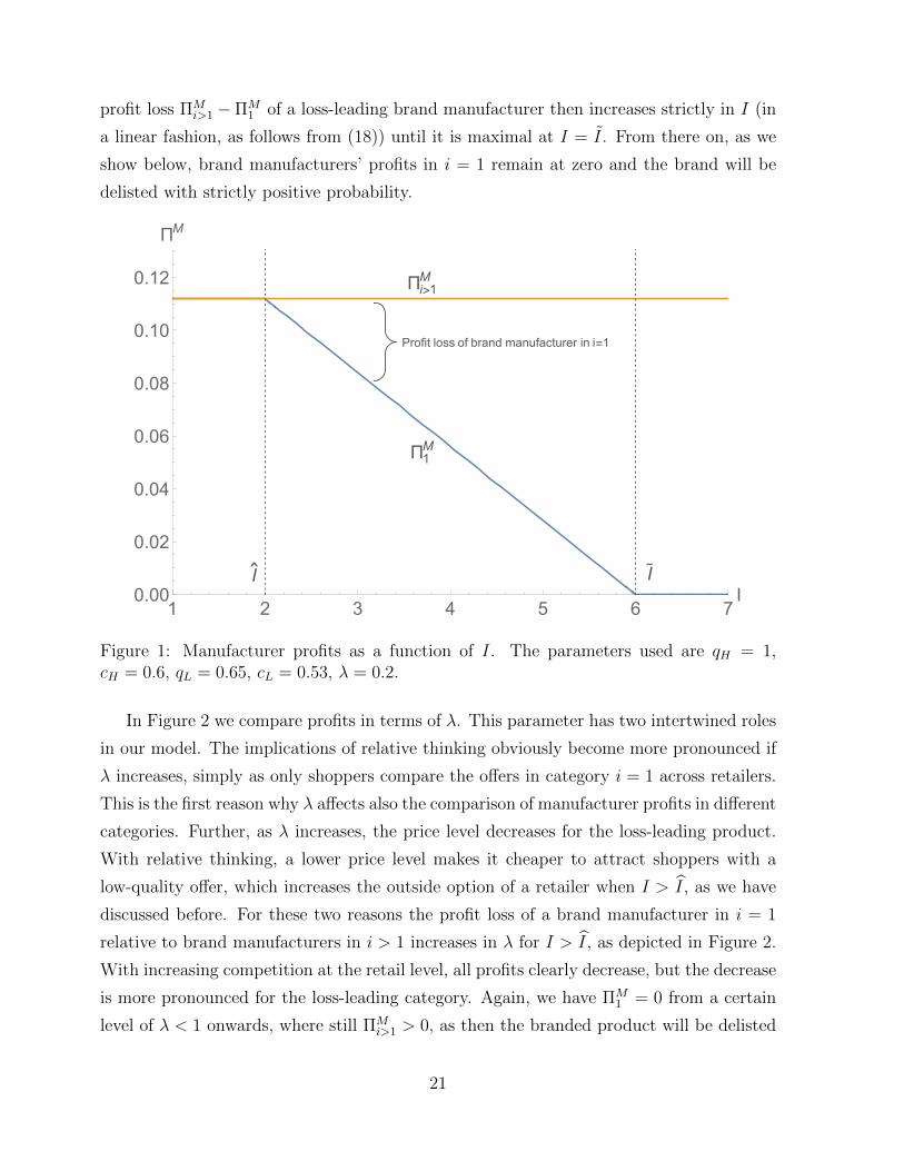
profit loss ΠMi>1 −ΠM
1 of a loss-leading brand manufacturer then increases strictly in I (in
a linear fashion, as follows from (18)) until it is maximal at I = I. From there on, as we
show below, brand manufacturers’ profits in i = 1 remain at zero and the brand will be
delisted with strictly positive probability.
1 2 3 4 5 6 7I0.00
0.02
0.04
0.06
0.08
0.10
0.12
ΠM
Profit loss of brand manufacturer in i=1
I
I˜
Π1M
Πi>1M
Figure 1: Manufacturer profits as a function of I. The parameters used are qH = 1,cH = 0.6, qL = 0.65, cL = 0.53, λ = 0.2.
In Figure 2 we compare profits in terms of λ. This parameter has two intertwined roles
in our model. The implications of relative thinking obviously become more pronounced if
λ increases, simply as only shoppers compare the offers in category i = 1 across retailers.
This is the first reason why λ affects also the comparison of manufacturer profits in different
categories. Further, as λ increases, the price level decreases for the loss-leading product.
With relative thinking, a lower price level makes it cheaper to attract shoppers with a
low-quality offer, which increases the outside option of a retailer when I > I, as we have
discussed before. For these two reasons the profit loss of a brand manufacturer in i = 1
relative to brand manufacturers in i > 1 increases in λ for I > I, as depicted in Figure 2.
With increasing competition at the retail level, all profits clearly decrease, but the decrease
is more pronounced for the loss-leading category. Again, we have ΠM1 = 0 from a certain
level of λ < 1 onwards, where still ΠMi>1 > 0, as then the branded product will be delisted
21

with positive probability in category i = 1. In sum, regardless of the reason why retail
competition intensifies in our model, a loss-leading brand manufacturer is affected strictly
more than manufacturers in other categories.
0.0 0.2 0.4 0.6 0.8 1.0λ
0.02
0.04
0.06
0.08
0.10
0.12
0.14
ΠM
Profit loss ofbrand manufacturer in i=1
Π1M
Πi>1M
Figure 2: Manufacturer profits as a function of λ. The parameters used are qH = 1,cH = 0.6, qL = 0.65, cL = 0.53, I = 4.
When consumers exhibit relative thinking, deep discounting and loss leading thus in-
deed hurt brand manufacturers, even when their products are still listed. They should
thus be particularly aware of the implications of intensifying retail competition. This is
even more so as the preceding discussion also suggests that, when such loss leading be-
comes sufficiently extensive, brand manufacturers may find their products delisted. For
completeness, we finally turn to this case.
5.3 The Threat of Being Delisted
When (16) no longer holds as I is too large, an equilibrium where both retailers always
stock the brand manufacturers’ product also in the loss-leading category no longer exists.
This is what we have already shown.
Note next that there can also not be an equilibrium where both retailers for sure
choose the low-quality (i.e., possibly store-brand) product in category i = 1. As profits
22
from shoppers are always fully competed away, the resulting (equilibrium) profits would
be strictly lower than when stocking a brand manufacturer’s product in i = 1 (at cost) and
targeting only non-shoppers.33 Hence, the equilibrium for product choice in the promoted
category must be in mixed strategies. We provide a characterization of the respective
probabilities in the proof of the subsequent proposition. There, we also characterize the
mixed pricing strategies.
Proposition 4 Suppose (16) does not hold. While brand manufacturers’ profits in all
other categories i > 1 are not affected, the brand manufacturers in the loss-leading category
make zero profit. With positive probability their products are no longer listed, and this
probability is higher when the extent of one-stop shopping I and thus discounts are larger.
Proof. See Appendix.
In our model, retailer discounting of a manufacturer’s own brand does not hurt the
manufacturer directly. In fact, such a direct impact on brand image might be more rel-
evant in the case of luxury goods, to which our model of sales and promotions may be
less applicable. Instead, in our model it is the overall lower price level that affects, via
consumers’ relative thinking, the relative perception of quality and price. As a conse-
quence, unless one brand manufacturer would virtually control the branded supply in a
given category, here i = 1, and could commit to impose a higher shelf price at all compet-
ing retailers, a single manufacturer can not successfully lean against loss leading and its
negative implications for all suppliers of branded products in the given category. This in-
sight can also be framed as follows. Consider just for now the image of competing vertical
chains – or, likewise, that of forward integrated manufacturers, who still face downstream
competition. Then, in any such vertical chain, downstream pricing and aggregate profits
would remain the same as in our analysis. And the same applies to the provision of high-
versus low-quality products. While such a picture is helpful to stress why an individual
branded goods manufacturer could not escape the described pitfall of low prices, for our
key result on the distribution of profits in the vertical chain it was necessary to consider
retailers and manufacturers separately. In our concluding remarks we now elaborate on
additional implications.
33In fact, the increase in profits resulting from such a deviation from the candidate equilibrium wouldbe (∆q −∆c)(1− λ)/2.
23
6 Conclusion
Our main empirical motivation comes from the observation that brand manufacturers,
notably of FMCG products, seem to resent retailers’ practice to heavily discount prices of
their products. As this should increase demand and as it is not obvious why manufacturers
should co-fund such promotions, this is at first puzzling. Our main result is therefore a
precise, formal derivation of the possible channel which explains this relationship. From
this we derive various implications, on which we now further expand.
We first recall the two main features of our model. First, with one-stop shopping
consumers base their choice of retailers only on the comparison of a selected number of
products. These are consequently the products on which price competition is fiercest.
Second, the relative weight that consumers give to different attributes of a product, here
price and quality, may depend on market circumstances, precisely on the relative difference
to other offers in the market. Our analysis captures these two features by combining a
model of one-stop stopping, set into a model of sales (Varian 1980), with insights from
the Marketing and Behavioral Economics literature on consumers’ relative perception of
quality and prices (“relative thinking”). Our main focus is on the implications for the
vertical layer, notably brand manufacturers’ profits.
The role of consumer preferences is crucial, as an increase in the extent of one-stop
shopping will only negatively affect manufacturer profits with relative thinking and not
with standard preferences. And this is the case only in the promoted (loss leading) cate-
gory. Thus, when consumers exhibit such relative thinking, but not so otherwise, we can
indeed support manufacturers’ concerns when retailers discount the respective product
category to compete for one-stop shoppers.
Brand manufacturers may have little influence on whether their product belongs to a
loss-leading category or not, which may depend, for instance, on whether it represents a
staple product that most households demand. Still, management can learn the following
from our analysis. Unless a manufacturer virtually controls the supply of branded products
in a given category, unilateral strategies of retail price maintenance, imposed either directly
or indirectly through the threat of withdrawing supply, can not shore up manufacturers’
profits. This is because it is the overall low price level in the promoted category that affects
consumers’ preferences over prices and quality. Instead, manufacturers would benefit when,
for instance, an industry-wide ban or restriction of loss leading was imposed, as it is the
case in some countries (at least for food retailing). If this is not the case and when the
24
category into which their main products fall is a typical loss leader, they should watch
out more carefully than other brand manufacturers for trends in retailing that could lead
to intensified retail competition. Looking backwards, this may indeed apply to the rise
of one-stop shopping. Looking into the future, online shopping even for staple grocery
products may further increase retail competition. In addition, online promotions of only
few items could increase the prominence of loss-leading strategies. When management
anticipates such changes, the return from an investment in brand value might fall. Then,
it may be more profitable to direct investments into cutting costs. We plan to explore
such longer-term strategic considerations of our model in future work.
7 References
Apffelstaedt, A., Mechtenberg, L. Competition for Context-Sensitive Consumers. Man-
agement Science, forthcoming.
Azar, O.H. Do People Think about Absolute or Relative Price Differences when Choosing
between Substitute Goods? Journal of Economic Psychology, 32(3): 450–457, 2011.
Bell, D., Lattin, J.M. Looking for Loss Aversion in Scanner Panel Data: The Confounding
Effect of Price Response Heterogeneity. Marketing Science, 19(2): 105–202, 2000.
Berges-Sennou, F., Bontems, P., Requillart, V. Economics of Private Labels: A Survey
of the Literature. Journal of Agricultural & Food Industrial Organization, 2: 1–25,
2004.
Bordalo, P., Gennaioli, N., Shleifer, A. Salience and Consumer Choice. Journal of Polit-
ical Economy, 121(5): 803–843, 2013.
Chandukala, S.R., Kim, J., Otter, T., Rossi, P., Allenby, G.M. Choice Models in Mar-
keting: Economic Assumptions, Challenges and Trends. Foundations and Trends in
Marketing, 2(2): 97–184, 2007.
Chintagunta, P. K., Bonfrer, A., Song, I. Investigating the Effects of Store-Brand In-
troduction on Retailer Demand and Pricing Behavior. Management Science, 10:
1242–1267, 2002.
Dertwinkel-Kalt, M., Lange, M., Kohler, K., Wenzel, T. Demand Shifts Due to Salience
Effects: Experimental Evidence. Journal of the European Economic Association, 15
25
(3): 626–653, 2017.
Diamond, W.D., Sanyal, A. The Effect of Framing on Choice of Supermarket Coupons.
Advances in Consumer Research, 17: 488–493, 1990.
Hastings, J. S., Shapiro, J. M. Fungibility and Consumer Choice: Evidence from Com-
modity Price Shocks. Quarterly Journal of Economics, 128 (4): 1449–1498, 2013.
Huber, J., Payne, J.W., Puto, C. Adding Asymmetrically Dominated Alternatives: Vio-
lations of Regularity and the Similarity Hypothesis. Journal of Consumer Research,
9(1): 90–98, 1982.
Inderst, R., Montez, J. Buyer Power and Dependency in a Model of Negotiations. RAND
Journal of Economics, 50(1): 29–56, 2019.
Inderst, R., Obradovits, M. Loss Leading with Salient Thinkers. RAND Journal of
Economics, 51(1): 260–278, 2020.
Inderst, R., Shaffer, G. Managing Channel Profits when Retailers Have Profitable Outside
Options. Management Science, 65(2): 642–659, 2019.
Kahneman, D., Tversky, A. Prospect Theory: An Analysis of Decision under Risk. Econo-
metrica, 47: 263–291, 1989.
Lal, R., Matutes, C. Retail Pricing and Advertising Strategies. Journal of Business, 67:
345–370, 1994.
Li, X., Gu, B., Liu, H. Price Dispersion and Loss-Leader Pricing: Evidence from the
Online Book Industry. Management Science, 59(6): 1290–1308, 2013.
Mills, D.E. Why Retailers Sell Private Labels. Journal of Economics and Management
Strategy, 4(3): 509–528, 1995.
Monroe, K.B. Buyers’ Subjective Perceptions of Price. Journal of Marketing Research,
10(1): 70–80, 1973.
Narasimhan, C. Competitive Promotional Strategies. The Journal of Business, 61(4):
427–449, 1988.
Simonson, I. Choice Based on Reasons: the Case of the Attraction and Compromise
Effects. Journal of Consumer Research, 16(2): 158–174, 1989.
26
Thaler, R.H. Mental Accounting and Consumer Choices. Marketing Science, 4(3): 199–
214, 1985.
Tversky, A., Kahneman, D. The Framing of Decisions and the Psychology of Choice.
Science, 211(4481): 453–458, 1981.
Varian, H.R. A Model of Sales. American Economic Review, 70(4): 651–659, 1980.
27
8 Appendix: Proofs
Proof of Proposition 1. To streamline the exposition of the proof, we first recognize
that, by the arguments in the main text, each retailer will stock high quality at categories
i > 1 and that the corresponding prices equal the respective valuation qH . We next
consider i = 1.
We argue to a contradiction and suppose qn = qL (suppressing for now the index
for i = 1). We next write expected demand at each retailer as a function of consumers’
(perceived) net surplus sn, which is sn = qL−pn, given the anticipated monopolistic pricing
at all products i > 1. Given the anticipated strategies at all other retailers n′ 6= n, in an
equilibrium retailer n faces some expected demand Xn(sn) (which, at this point, we need
not derive explicitly). Take now some equilibrium price pn (i.e., a price for i = 1 in the
respective support of retailer n) and expected demand Xn(qL − pn). Consider a deviation
to qn = qH and the choice of a price pn = pn + ∆q, which thus realizes the same expected
demand. In case the high-quality manufacturer offered his product at the wholesale price
wn = cH , the retailer’s increase in profit (gross of Tn) would then be at least
κ =1− λN
(∆q −∆c) > 0.
By setting Tn = κ/2 the respective high-quality manufacturer can thus ensure that its
(deviating) offer is accepted for sure and that it generates strictly positive profits, which
results in a contradiction to the claim that retailer n offers low quality for product i = 1.
We next turn to wholesale contracts. We wish to support an equilibrium where marginal
wholesale prices equal marginal costs. Take first i = 1 and note that, at retailer n, the
respective price p1n, where we now make the dependency on i = 1 explicit, then maximizes[
(p1n − w1
n) + (I − 1)(qH − cH)]Xn(qH − p1
n), (19)
so that joint profits of retailer n and the respective high-quality manufacturer are clearly
maximized when w1n = cH . This extends also to the providers of products i > 1 as follows.
Then, the respective objective function of the retailer equals[(p1n − cH) + (I − 2)(qH − cH) + (qH − win)
]Xn(qH − p1
n), (20)
which equals that in (19).
28
Next, given marginal wholesale prices equal to marginal manufacturer costs, the de-
termination of fixed fees follows from the argument in the main text as follows. For this
we show that when a retailer rejects the offer of the high-quality manufacturer of any
category i, the deviation profit, gross of the fixed fees T jn for all other manufacturers j, is
obtained by attracting only the respective locked-in fraction of consumers. We show this
first when i = 1. Consider generally any two levels of net utility that a retailer may offer
to consumers, s′ < s′′. We show that when offering s′ is weakly preferred for a retailer
that (on-equilibrium) chooses q1n = qH , offering the lower net utility is strictly preferred
when the retailer deviates to qn = qL. Formally: Making use of the expression Xn(s) for
expected demand, as well as prices p′H = qH − s′ and p′′H = qH − s′′ with high quality and
prices p′L = qL − s′ and p′′L = qL − s′′ with low quality, we claim that
[(qH − s′ − cH) + (I − 1)(qH − cH)]Xn(s′) ≥ [(qH − s′′ − cH) + (I − 1)(qH − cH)]Xn(s′′)
implies
[(qL − s′ − cL) + (I − 1)(qH − cH)]Xn(s′) > [(qL − s′′ − cL) + (I − 1)(qH − cH)]Xn(s′′),
which indeed holds from ∆q > ∆c.34 As we already know that offering zero net utility
(pn = qH) yields the equilibrium profits, offering zero net utility (now pn = qL) must then
indeed be uniquely optimal when deviating to qN = qL. From the respective expressions
for π, we then obtain from a retailer’s indifference, which must hold by optimality for the
manufacturer, that
T 1n = (∆q −∆c)
1− λ2
.
We can now apply this argument also to all categories i > 1, after noting the equivalence
of the respective expressions as used already when we compared (19) with (20). Q.E.D.
Proof of Proposition 2. The equilibrium characterization is a straightforward extension
from the case where consumers all have the same reservation value of shopping (of zero).
We thus already make use of the observations that, first, for all products the high quality
34More precisely, when we impose equality on the first condition, we can write this as
[(qL − s′ − cL + [(qH − cH)− (qL − cL)]) + (I − 1)(qH − cH)]Xn(s′) =
[(qL − s′′ − cL + [(qH − cH)− (qL − cL)]) + (I − 1)(qH − cH)]Xn(s′′), i.e.,
[(qL − s′ − cL) + (I − 1)(qH − cH)]Xn(s′) =
[(qL − s′′ − cL) + (I − 1)(qH − cH)]Xn(s′′) + (∆q −∆c) [Xn(s′′)−Xn(s′)] .
From this, our second inequality follows as ∆q > ∆c and as clearly Xn(s′′) > Xn(s′).
29
is stocked and, second, there is an equilibrium where marginal wholesale prices equal
marginal costs.
Observe next that a retailer’s expected (gross) profit with any non-shopping local
consumer is
π = (p− cH + (I − 1)(qH − cH))G(qH − p). (21)
We suppose for convenience that g/G is weakly increasing in its argument, so that pm =
arg maxp π is uniquely determined and results in (per-consumer) expected profits of πm.
Thus, when a retailer only attracts non-shoppers, then the maximum profit is 1−λ2πm (gross
of any fixed fee paid to the manufacturer).
We turn now to the derivation of manufacturer profits. Take i = 1 with respective
profits ΠM1 . From the respective indifference condition for each retailer, we now have
ΠM1 =
1− λ2
(πmH − πmL ) ,
where we extended the notation in (21) as follows: πmH denotes the maximum profit when
the retailer stocks qH at cost cH and πmL is the respective maximum profit when the
retailer instead stocks qL at cost cL. Using uniqueness of the respective prices pMH an pML
and appealing to the envelope theorem, we have that
dΠM1
dI= (qH − cH)
1− λ2
[G(qH − pmH)−G(qL − pmL )] .
To show that profits increase with the extent of one-stop shopping, it thus remains to
prove that
pmH − pmL < ∆q. (22)
To see this, it is now convenient to denote more generally pm(q, c) as the “monopoly price”
when, at i = 1, quality q is stocked at cost c. With this we rewrite
pmL = arg maxp
[(p− cL + (I − 1)(qH − cH))G(qL − p)]
= arg maxp
((p−∆q)− cL + (I − 1)(qH − cH))G(qL − (p−∆q))−∆q
= pm(qH ,∆q + cL)−∆q.
Hence, the requirement (22) transforms to
pmH = pm(qH , cH) < pm(qH ,∆q + cL),
which follows as, when this is interior for a non-degenerate G(·), ∂pm(q, c)/∂c > 0 and as
∆q + cL > cH from ∆q > ∆c.
30

With respect to manufacturer profits, it remains to prove that, with elastic demand,
ΠM1 > ΠM
i for i > 1. To see this, we have to derive ΠMi , appealing again to retailer
indifference. For this we make again use of expression (21) as follows. On equilibrium,
the retailer’s gross profits are 1−λ2πm. Off equilibrium, after rejecting the offer of one
manufacturer in some category i > 1, the retailer’s maximum profits are again obtained
by targeting only non-shoppers and choosing the respective optimal “monopoly” price p,
thereby now realizing (per consumer)
maxp
(p− cH + (I − 2)(qH − cH) + (qL − cL))G(qH − p).
We denote these per-consumer profits by πmH,L, indicating that high quality is offered in
category 1 (as well as in I − 2 additional categories), while in one (non loss-leading)
category low quality is offered. Consequently, we have for i > 1
ΠMi =
1− λ2
(πmH − πmH,L
),
so that ΠM1 > ΠM
i holds if πmH,L > πmL , i.e. if
maxp
(p− cH + (I − 1)(qH − cH))G(qL − p) (23)
< maxp
(p− cH + (I − 2)(qH − cH) + (qL − cL))G(qH − p).
Recall that the maximizer of the first expression is denoted by pmL . Clearly, the second
expression is bounded from below when we substitute some price p′ = pmL + ∆q, so that
G(qH − p′) equals G(qL − pmL ). Note finally that for this price choice we have
p′ − cH + (I − 2)(qH − cH) + (qL − cL)
= pmL − cH + (I − 1)(qH − cH).
For completeness we finally extend our characterization of the pricing equilibrium. Both
retailers randomize according to some continuous CDF F (p) over the support p ∈ [p, pm].
A retailer choosing p = p can be certain to sell to all shoppers whose reservation value is
sufficiently low, while with p = pm the retailer sells only to its local non-shoppers (with
sufficiently low reservation value). To make the retailer indifferent between these two
choices, p must satisfy(1− λ
2+ λ
)(p− cH + (I − 1)(qH − cH))G(qH − p) =
1− λ2
πm, (24)
31
while the distribution F (p) is finally obtained from the requirement to make each retailer
indifferent also with respect to all p ∈ (p, pm):
F (p) = 1− 1− λ2λ
[πm
(p− cH + (I − 1)(qH − cH))G(qH − p)− 1
]. (25)
Q.E.D.
Proof of Proposition 3. We first consider a candidate equilibrium of high quality in all
categories. For this we determine a retailer’s deviation profits. Suppose thus that retailer
n, instead of choosing qn = qH in category i = 1, deviates to qn = qL. Then, given the
rival retailer’s anticipated choice of qn′ = qH in the same category and the corresponding
product price drawn from F (·), as given in (7), when setting an arbitrary price pL retailer
n makes an expected deviation gross profit of
πn(pL; qL) = [pL − cL + (I − 1)(qH − cH)]
[1− λ
2+ λ(
1− F(pLqHqL
))]=
[pL − cL + (I − 1)(qH − cH)]1−λ2I(qH − cH)
qHqLpL − cH + (I − 1)(qH − cH)
,
where the second equality follows from inserting F (·), and simplifying. It now holds that∂πn(pL;qL)
∂pLhas the same sign as
η(I) ≡ qHqLcL − cH − (I − 1)(qH − cH)
∆q
qL,
which is, in particular, independent of pL. Hence, the deviation gross profit πn(pL; qL) is
monotonic in pL. If η(I) ≥ 0, which is equivalent to
I ≤ qH∆q
(∆q −∆c
qH − cH
)= I ,
the optimal deviation price is the highest feasible price pL = qL, yielding thus a maximal
deviation gross profit of
πn(qL; qL) = [qL − cL + (I − 1)(qH − cH)]1− λ
2.
If instead η(I) < 0 (I > I), the optimal deviation price is qLqHp, which guarantees that all
shoppers are attracted. The corresponding deviation gross profit is then
πn(qLqHp; qL) = [
qLqHp− cL + (I − 1)(qH − cH)]
1 + λ
2.
32
Depending on the sign of η(I), or likewise on how I compares to the threshold I, we have
thus derived the optimal deviation pricing strategy and from this corresponding profits
when a retailer deviates to qL in category i = 1. Recall now that a brand manufacturer
in i = 1 can extract as fixed fee (and thereby, profit) the difference of the retailer’s gross
profit when stocking qH at the marginal wholesale price cH ,
πn(qH) = (qH − cH)I1− λ
2= [p− cH + (I − 1)(qH − cH)]
1 + λ
2,
and the retailer’s maximal deviation profit. Hence, when I ≤ I, the brand manufacturer
of i = 1 makes a profit of
ΠM1 = (qH − cH)I
1− λ2− [qL − cL + (I − 1)(qH − cH)]
1− λ2
= (∆q −∆c)1− λ
2,
i.e., the same as other brand manufacturers. But when I > I, the brand manufacturer of
i = 1 makes a profit of
ΠM1 = [p− cH + (I − 1)(qH − cH)]
1 + λ
2− [
qLqHp− cL + (I − 1)(qH − cH)]
1 + λ
2
=1 + λ
2(∆q −∆c)− Iλ
∆q
qH(qH − cH),
which is strictly lower than other brand manufacturers’ profits of (∆q−∆c)1−λ
2. Moreover,
in this case ΠM1 is clearly strictly decreasing in I, as claimed.
Note finally that from the preceding derivation of a deviating retailer’s maximum prof-
its, we immediately obtain the respective equilibrium condition (16). Q.E.D.
Proof of Proposition 4. In what follows, we provide a full characterization of the
equilibrium strategies, which implies the statements in the proposition.
Lemma 1 If the converse of (16) holds such that I > I, no equilibrium exists in which both
retailers stock the branded product or the low-quality product in category i = 1 with proba-
bility one. There exists a unique symmetric equilibrium involving mixed product strategies
such that either retailer stocks the branded product in i = 1 with probability
α∗ =1− λ
2λ
[(∆q −∆c)qH
(I − 1)(qH − cH)∆q + qLcH − qHcL
]∈ (0, 1),
where α∗(I) = 1 and α∗(I) strictly decreases as the extent of one-stop shopping I increases.
The equilibrium pricing strategies are as follows. Conditional on stocking qH in i = 1, a
33
retailers draws his price in i = 1 from the CDF
FH(pH) = 1− 1
α∗
[1− λ
2λ
(qH − pH
pH − cH + (I − 1)(qH − cH)
)](26)
with support
[pH, pH ] =
[∆c
∆q
qH , qH
].
Conditional on stocking qL in i = 1, a retailer draws his price in i = 1 from the CDF
FL(pL) =1− 1−λ
2λ
(qH−∆c−pL
pL−cL+(I−1)(qH−cH)
)1− α∗
(27)
with support
[pL, pL] =
[p−∆c,
∆c
∆q
qL
],
where p is given in (6). In this equilibrium, brand manufacturers in i = 1 charge no fixed
fee and consequently make zero profit.
Proof. Recall from the main text that for I > I no equilibrium exists in which both
retailers stock the branded product in i = 1 for sure or where both retailers stock the
low-quality quality product in i = 1 for sure. In what follows, we confine ourselves to
proving existence of the outlined symmetric mixed-strategy equilibrium in product choice
(and pricing). The proof for why this is also the unique symmetric equilibrium is slightly
more subtle and is available from the authors upon request.
For existence, note first that when retailers stock different products in i = 1 in the
candidate equilibrium, then firms’ price distributions are such that qH/pH < qL/pL with
probability one (as qH/pH = qL/pL, pH ≥ pH
and pL ≤ pL). Hence, a retailer stocking
qH in i = 1 (at marginal wholesale price cH) and setting some price pH ∈ [pH, pH ] only
attracts the shoppers if its rival stocks the high-quality product as well and chooses a price
higher than pH (joint probability α∗(1 − FH(pH))). Therefore, such a retailer’s expected
gross profit is given by
πn(pH ; qH) = [pH − cH + (I − 1)(qH − cH)]
[1− λ
2+ λα∗(1− FH(pH))
]= (qH − cH)I
(1− λ2
),
where the second equality follows from inserting FH(·), and simplifying. If instead a
retailer stocks qL in i = 1 and sets some price pL ∈ [pL, pL], the retailer attracts the
shoppers whenever the rival stocks qH in i = 1 (probability α∗) or when the rival stocks
34
qL in i = 1 and chooses a price higher than pL (joint probability (1 − α∗)(1 − FL(pL))).
Therefore, such a retailer’s expected gross profit is given by
πn(pL; qL) = [pL − cL + (I − 1)(qH − cH)]
{1− λ
2+ λ [α∗ + (1− α∗)(1− FL(pL))]
}= [pL − cL + (I − 1)(qH − cH)]
{1− λ
2+ λ [1− (1− α∗)FL(pL)]
}= (qH − cH)I
(1− λ2
)= πn(pH ; qH),
where the second equality follows from inserting FL(·), and simplifying. As a first impli-
cation, note that the retailers are indeed indifferent between stocking qH in i = 1 and
setting any price pH ∈ [pH, pH ], or stocking qL in i = 1 and setting any price pL ∈ [p
L, pL].
A further implication from this indifference is that brand manufacturers can indeed not
charge a positive fixed fee. Further, retailers can not profitably deviate by stocking qH in
i = 1 and pricing above pH = qH (as this would imply zero demand) or stocking qL in
i = 1 and pricing below pL
(as already by setting pL = pL, the shoppers are attracted with
certainty). It remains to show that the retailers do not wish to deviate by stocking qH in
i = 1 and pricing strictly below pH
(giving them a chance to attract the shoppers even
when the rival stocks qL in i = 1) or by stocking qL in i = 1 and pricing strictly above pL
(risking to lose the shoppers also when the rival chooses qH in i = 1, but realizing a higher
margin on each sale of i = 1). We prove this next.
To see the former, note that for pH < pH
a retailer’s expected gross profit is given by
πn(pH ; qH) = [pH − cH + (I − 1)(qH − cH)]
[1 + λ
2− λ(1− α∗)FL
(pH
qLqH
)],
as the mass λ of shoppers is attracted unless the rival stocks low quality in i = 1 and prices
below pHqLqH
(joint probability (1−α∗)FL(pH
qLqH
)). Plugging in FL(·) and simplifying yields
πn(pH ; qH) = [pH − cH + (I − 1)(qH − cH)]
(1− λ
2
)(I(qH − cH)
pHqLqH− cL + (I − 1)(qH − cH)
)
for pH < pH
. The derivative of πn(pH ; qH) with respect to pH has the same sign as
qLcH − qHcL + (I − 1)(qH − cH)∆q.
This is strictly positive for I > I, which is true since by assumption I > I, and it holds
that I > I. We have thus shown that it is indeed not profitable to deviate to prices pH
35
below pH
. If instead a retailer stocks qL in i = 1 and chooses a price pL ∈ (pL, qL], its
expected gross profit is
πn(pL; qL) = [pL − cL + (I − 1)(qH − cH)]
[1− λ
2+ λα∗
(1− FH
(pLqHqL
))],
as the mass λ of shoppers is only attracted when the rival retailer stocks qH and chooses
a price that exceeds pLqHqL
(joint probability α∗(1 − FH
(pL
qHqL
))). Inserting FH(·) and
simplifying yields
πn(pL; qL) = [pL − cL + (I − 1)(qH − cH)]
(1− λ
2
)(I(qH − cH)
pLqHqL− cH + (I − 1)(qH − cH)
)
for all pL ∈ (pL, qL]. The derivative of πn(pL; qL) with respect to pL now has the same sign
as
−[qLcH − qHcL + (I − 1)(qH − cH)∆q],
which is strictly negative as I > I > I. Hence, also deviation prices pL above pL are not
profitable. Taken together, we have thus shown that the outlined symmetric strategies
indeed constitute an equilibrium, while no equilibrium exists where in i = 1 either the
high- or the low-quality product is chosen with probability one. We finally note that all
CDFs and probabilities used in the construction of the equilibrium are indeed well-behaved
as follows: α∗(I) = 1 (as is easy to check), so that α∗(I) ∈ (0, 1), which is also strictly
decreasing in I for I > I; FH(pH
) = FL(pL) = 0; FH(pH) = FL(pL) = 1; and FH(pH)
and FL(pL) are strictly increasing in their arguments for pH ∈ [pH, pH ] and pL ∈ [p
L, pL],
respectively.
Q.E.D.
36