Why Do Guaranteed SBA Loans Cost Borrowers So

Much?∗

Flavio de Andrade†

Northwestern UniversityDeborah LucasMIT and NBER

September 1, 2009

Abstract

The SBA assists small businesses in obtaining access to bank credit by guaranteeing a portionof their loans. Despite the substantial federal guarantee and a history of modest default rates,borrowers are charged rates similar to those on low-grade bonds. We suggest several possibleexplanations for this phenomenon, including lack of competition between SBA lenders, and arelatively high cost of insured capital for guaranteed loans. Using comprehensive data obtainedfrom SBA on all disbursed loans from 1988 to 2008, we find some evidence of market powerin that large lenders charge borrowers relatively high rates. To evaluate the cost of capital onthe guaranteed portion of SBA loans, we develop a Monte Carlo model of the cash flows onfully guaranteed SBA securitized pools, taking into account historical default and prepaymentpatterns. Comparing our model predictions to market prices provided by large dealer in SBApools, we find that investors required a spread between 100 and 200 bps over the Treasury curveto hold these securities.

Keywords: Credit subsidy, government guarantee, banking competition, and securi-tization.

JEL Classification: D4, G2, and H8.

∗We thank Lamont Black, Fritz Burkardt, Renato Gomes, Ravi Jagannathan, Jennifer Main, Damien Moore, SylviaMerola, Jonathan Parker, Rafael Rogo, Niels Schuehle, Neil Wiggins and especially Wendy Kiska for their commentsand help with obtaining and understanding the data used in this project. We also thank seminar participants at theFederal Reserve Bank of Cleveland and at the 2009 American Economic Association Annual Meetings. All errorsremain our own.

†Northwestern University, 2001 Sheridan Road, Evanston, IL 60208. Email:fjr@kellogg.northwestern.edu

1

1 Introduction

The federal government increasingly relies on subsidized credit guarantees in lieu of grants or other

forms of assistance to targeted groups. In providing credit assistance, the government has a choice

between direct lending where it funds loans directly via the Treasury, and guaranteed lending

where funds are raised indirectly via private financial institutions in the capital markets. Whether

guaranteed lending is an efficient way of subsidizing credit is an important question that we explore

here in the context of the Small Business Administration’s (SBA) 7(a) program.

The goal of the SBA 7(a) program is to lower the cost and improve the availability of credit

to U.S. small businesses. In 2006, it guaranteed 82,000 loans totaling $12 billion. The loans

generally have an original maturity of 7 to 25 years, and interest is based on the prime rate plus

a fixed spread. Qualified borrowers are able to obtain loans from SBA-certified private financial

institutions, usually commercial banks, with the backing from a federal guarantee that insures the

lender against 50 to 85 percent of credit losses.

One of the arguments to justify guaranteed lending programs is that private institutions have

better screening skills than the government. The SBA only provides partial guarantees, leaving

banks with some default risk and inducing them to pick out qualified borrowers. The minor historic

default rates confirm that private lenders are indeed motivated by the right screening incentives. As

a result, the government is subject to the tradeoff between efficient screening versus the potential

rent transfers from borrowers to lenders.

Despite the benefit of a substantial federal guarantee and default experience that is no worse

than that on seemingly comparable loans and bonds, 7(a) borrowers are charged rates that are

no lower than on comparable uninsured securities. In this paper we review the evidence that

supports this conclusion, and evaluate several possible explanations for why borrowers are charged

such seemingly high rates. One hypothesis is that high borrowing rates are a consequence of

imperfect competition in the 7(a) lending market, making the loans a profitable line of business for

participating lending institutions. In 2006 more than 2000 lenders originated SBA-backed loans.

Some of the banks originate large numbers of 7(a) loans, while others choose not to participate in

the program at all, and in some regions there are very few SBA lenders.

2

To examine the hypothesis that high costs are due to limited competition, we first study the

effect of regional banking concentration on interest rates. We calculate a measure of local SBA

lender concentration based on a Herfindahl index and regress interest rate spreads on Herfindahl

index values, controlling for observable borrower and loan characteristics. We find no evidence that

rate spreads increase with lender concentration, and in fact consistently find the opposite. We then

consider an alternative to the Herfindahl index, based on the cross-section of bank size. We assign

each bank to a size category based on the number of loans originated in a given year. According to

this classification we find that the largest lenders tend to charge higher spreads than smaller ones,

even after controlling for default and prepayment.

High borrowing rates for 7(a) borrowers may also be attributable to a higher cost of insured

capital for 7(a) lenders than what one would expect with a full faith and credit federal guarantee.

Past studies have shown that federally guaranteed obligations such as RTC bonds and student loans

bear higher rates than standard Treasury securities despite full faith and credit federal guarantees,

and that the rate differences can be substantial (Longstaff (2004) [7], Lucas and Moore (2009) [8]).

These authors point to lower liquidity as a likely reason for the higher required rates of return than

on comparable Treasury’s.

In evaluating the rate charged on 7(a) loans, one has to take into account that 7(a) loan cash

flows are risky, despite being guaranteed against default risk.1 There is considerable uncertainty

as to the timing of payments because of the possibility of default and prepayment, and due to

movements in the prime rate. This can introduce systematic risk into cash flows even though direct

losses from default are precluded. The additional layers of intermediation introduced by relying on

banks and securitization markets also create additional costs that can elevate spreads.

To evaluate the cost of capital on the guaranteed portion of SBA loans, we develop a Monte Carlo

model of the cash flows on such securities, taking into account historical default and prepayment

behavior, and modeling interest rates using a two-factor Cox, Ingersoll and Ross (CIR) [2] model.

Discounting these cash flows at the risk-free rates along each path, we find the theoretical value

of the cash flows at Treasury rates. By comparing these theoretical prices to actual secondary

market prices of the securitized pooled and guaranteed portion of SBA loans, we can then infer the

spread over Treasury rates necessary to equate the theoretical price with the market price. We find

1This is also true of other federally guaranteed loans such as FHA loans and student loans.

3

evidence that investors typically demand a spread between 100 and 200 bps over Treasury rates in

the period for which we have data (1/06 through 6/08), which explains part of why 7(a) loans cost

borrowers so much despite the benefit of a federal guarantee.

A lending market with a large number of banks is not necessarily competitive (Wolinsky 1986

[14], Stiglitz 1979 [11]), and as a result lenders may not lower interest rates when they obtain

loan insurance. In fact, lenders may optimally increase the interest rates and lend more to riskier

borrowers when the percent guaranteed rises. These considerations lie beyond the scope of this

paper and will be pursued in future research. Our analysis focuses on a cost-based approach which

evaluates the level of interest rates that banks could charge if the market for SBA loans was assumed

to be perfectly competitive.

The rest of the paper is organized as follows: Section 2 gives a brief overview of the 7(a) program.

Section 3 presents evidence that 7(a) loans appear relatively expensive for borrowers, and also very

profitable for lenders. Section 4 reports on how borrower characteristics, loan characteristics, and

the concentration among SBA lenders are related to the cross-section of credit spreads. In Section

5 we develop the model to price SBA guaranteed loan pools, and compare model prices with market

prices to infer the premium over Treasury rates demanded by investors. The likely profitability of

SBA loans is reevaluated given this information. We conclude in Section 6 with a discussion of the

policy implications of the findings.

2 SBA 7(a) Program Overview

In this section we briefly describe the most salient features of the 7(a) lending program for this

analysis, since more complete descriptions are available elsewhere (e.g., CBO (2000) [10] and Glen-

non and Nigro (2005) [5]). In terms of total size, the program that has grown rapidly since 2001,

with $12 billion in principal disbursed on more than 82,000 loans in 2006. Still, 7(a) loans rep-

resent less than 5 percent of total U.S. small business borrowing. What we refer to as the 7(a)

program actually has two parts, a regular program and an “Express” program. The Express pro-

gram promises borrowers and lenders quick eligibility decisions, but provides a federal guarantee

on only 50% of loan principal and has a stricter restriction on loan size. The Express program has

grown to represent near 75 percent of loans guaranteed, but only 20 percent of dollar loan volume.

4

2.1 Borrowers

Businesses seeking 7(a) loans must satisfy a number of criteria. The most subjective is that they

must establish that they have not been able to obtain credit elsewhere on “affordable terms.” They

also must demonstrate an ability to repay the loans, for instance based on collateral, the amount of

owners’ equity, and the general quality of management.2 More concretely, the business must be for-

profit, small (the definition varies by industry), and independently owned and operated. Borrowers

come from a wide variety of industries, with the largest three being retail trade, accommodation and

food services, and manufacturing, which together account for about 50 percent of loans disbursed.

2.2 Loan Terms and Characteristics

Over 96 percent of 7(a) borrowers pay an interest rate set to a fixed spread over the prime rate.

The prime rate is a floating rate that since 2000 has hovered around 3 percent above the overnight

Fed Funds rate. The spread is capped by SBA regulation, but on most loans the spread cap does

not appear to bind. There are also a variety of fees assessed by the SBA, some paid by the borrower

directly and others by the lender. Borrowers pay a graduated one-time guarantee fee that ranges

from 2 percent of principal for loans of less than $150,000 to 3.5% for loans of $1 million. Borrowers

with long-term loans also face high prepayment penalties in the first three years of the loan’s life,

after which prepayment is a free option. Lenders pay the SBA an annual servicing fee of .545

percent on the guaranteed balance, although they bear most servicing costs themselves.

Loan maturity typically is 7 to 10 years, but varies with the purpose of the loan. Loans for

real estate and equipment may extend to 25 years. The effective duration of loans is considerably

shorter, both because the loans are amortizing and because of voluntary prepayments and defaults.

Loans in the regular program can be for up to $2 million, and in the Express program up to

$350,000.

The maximum percentage guaranteed varies with the loan size and program. In the regular

program, for loans under $150,000, SBA guarantees up to 85% and for loans above $150,000 the

maximum is 75%. On Express loans the maximum guarantee percentage is 50%. Loans do not

always bear the maximum allowable guarantee, presumably to reduce the amount of fees paid to

SBA. Upon default, a lender can recover from SBA the face value of the outstanding principal bal-

2The SBA assigns a risk rating to individual loans, but it is not a standard credit score and that data is proprietary

5

ance, and subsequently will receive a pro rata share of any recoveries. However, lenders sometimes

choose not to exercise the guarantee when they expect to recover more from retaining the entire

loan. Thus the SBA default statistics that we rely on are somewhat downward-biased estimates of

the default rate experienced by the borrower.3

2.3 Lender Characteristics

SBA-backed loans are typically made by commercial banks, but some thrifts and finance companies

also participate. Lenders classified by SBA as “preferred lenders” have the authority to determine

eligibility in the Express program. For commercial banks, an advantage of participation is that

it helps to satisfy Community Reinvestment Act requirements. As described in more detail in

section 4, relatively few banks4 originate large numbers of 7(a) loans. Of 2017 distinct lending

organizations identified for 2006, only 13 originated more than 1,000 loans each, and 880 originated

only 1 or 2 loans. The identities of the 20 largest originators and their lending volume are shown

in Table 1.

2.4 The Guaranteed Loan Pool Certificate Program (GLPCP)

To increase access to capital for 7(a) lenders, since 1995 the SBA has sponsored the Guaranteed

Loan Pool Certificate Program (GLPCP). Under this program 7(a) lenders can sell the guaranteed

portion of 7(a) loans to a Pool Assembler. The Assembler puts together pools of loans that are

similar in terms of maturity, rate basis (e.g., monthly and prime-based), and rate spread. Each pool

has a minimum of four underlying loans that total at least $1 million in aggregate. The strictest

restrictions on rate floors or ceilings on the individual loans are reported for the pool. The pools

are sold via an auction to investors, and there is also a secondary market in the Certificates.

It appears that the securitization process does not introduce any significant counterparty risk

into the lending process. Payments on the securities are centralized and made by Fiscal and

Transfer Agent (FTA-Colson Associates), who is appointed by the government and acts as their

agent. Payments are made on time even when default and prepayments occur. These payments

are made by the FTA to investors in the form of advances. Lenders also do not bear counterparty

3For the purposes of calculating returns to lenders, this problem is mitigated by the fact that non-surrenderedloans are those with relatively high recovery rates.

4A bank for this tabulation consolidates over institutions governed by the same holding company, even if theyoperate in far flung geographic regions.

6

risk either since they deal directly with the FTA.

The program has become an increasingly important source of financing, with a $4.0 billion of

guaranteed securities sold into pools in 2006, representing 42% of the total guaranteed amount of

loans approved in that year. We have no evidence on whether securitized loans deviate systemati-

cally from a typical SBA loan in terms of default or prepayment behavior. We assume that there is

no significant selection bias since they represent a large fraction of total originations. The market

prices of these certificates is of interest in this analysis because they can be used to infer the cost

of capital for the default-risk-free portion of 7(a) loans, as discussed in Section 5 below.

3 The Cost and Profitability of 7(a) Loans

Our inferences about the cost of SBA loans rely on comprehensive data obtained from SBA on

all disbursed loans from 1988 to 2008. Associated with each loan is static information about the

borrower (e.g., type and size of business), the lender (e.g., name, state), and loan terms (e.g., rate

spread, basis, maturity, if collateral). There is also a record of prepayments and defaults. The SBA

loan data is described in more detail in Appendix 1.

3.1 Cost to Borrowers

Average rate spreads and guaranteed shares on 7(a) loans are summarized in Table 2. The average

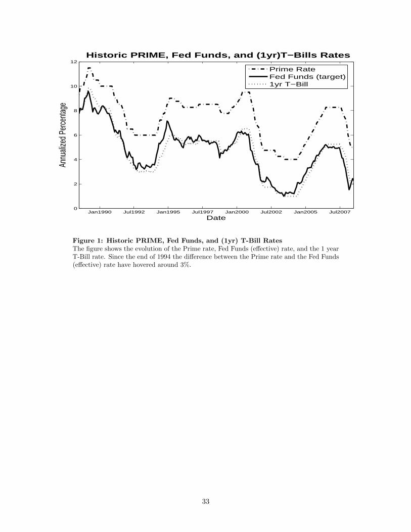
spread over prime is 2.46%, based on all loans disbursed from 1988 and 2008. Over the sample

period the prime rate averaged 2.77% over the overnight Fed Funds rate5 , and the level of the Fed

Funds rate was roughly equivalent to the 1-year Treasury rates (see Figure 1). Thus on average

borrowers paid a spread of about 5.23% over the 1-year Treasury rate, even though the average

loan bore a federal guarantee on 68.6% of principal. The initial guarantee fee added about 40 bps

to the effective rate paid by borrowers6.

To assess whether these spreads are in line with other credit obligations with comparable default

risk, we draw on the analysis in CBO (2007), which uses the same SBA loan data. Figure 2

(reproduced from CBO (2007), Figure 4) shows that the spread charged SBA borrowers has been

consistently higher than that for all commercial and industrial (C&I) loans by a margin of about

two percentage points for regular 7(a) loans, and over three percentage points for Express loans.

5Fed Funds is used as a reference point because since 2000 the prime rate has been fixed at 3% over Fed Funds.6This assumes a 2.5% guarantee fee, a 7-year initial maturity, and a discount rate of 7%.

7

Higher rates on SBA loans might be justified, even with a partial guarantee, if the probability

of default is significantly higher than on other C&I loans. The most direct evidence that it is not

higher comes from, Glennon and Nigro (2005), who find that, although medium-maturity loans

originated under the SBA 7(a) loan guarantee program are targeted to small firms that fail to

obtain credit through conventional channels, the default experience is comparable to that of a large

percentage of loans held by larger commercial banks. Further evidence on default rates is found

by comparing the cumulative default rates on 7(a) loans and public debt. CBO (2007) finds that

the default experience on 7(a) loans falls between that on BB and BBB-rated bonds (see Figure 3,

reproduced from Figure 9 in CBO (2007)). Figure 4 shows that overall default rates on 7(a) loans

have fallen over time, and have stabilized at just less than 2 percent of principal outstanding since

1995. Netting the average recovery rate of between 40 and 50 percent suggests an annual loss rate

to SBA of about 1 percent.

3.2 Returns to Lenders

The value of 7(a) loans from a lender’s perspective depends on the margin between revenues and

costs. Revenues arise from borrower payments and proceeds from loan sales. Costs include the

lender’s weighted average cost of funds, servicing and other ongoing administrative costs, and fees

paid to the SBA. Taking these costs into account, we do a simple back-of-the-envelope calculation

in this section suggesting that 7(a) loans on average are quite profitable for banks.

For bank lenders, holding a 7(a) loan is like owning a portfolio of a default-risk-free government

security and a risky small business loan. Banks’ weighted average cost of capital for 7(a) loans

should reflect these two components, and in a competitive market the advantage of the guarantee

should be passed through to the borrower. The cost of funds is clearly different for the insured

and uninsured portions of a loan. The insured portion is virtually default-risk free, suggesting that

investors would require a return close to a short-term risk-free Treasury rate on a floating rate

loan7. (In Section 5 we present a more careful analysis of the cost of funds for the guaranteed

portion.) On the uninsured portion, default experience suggests funding costs similar to those on

BB to BBB-rated loans. Based on historical BB rate spreads, the gross funding rate on the risky

portion is taken to be Treasury + 3.5 percent. This is also consistent with the spread between C&I

7Consistent with this view, banks investing in GLPCP certificates have a 0% capital requirement against theseholdings.

8

loans and SBA loans in Figure 2. Based on an average 68.6% of guaranteed principal, the WACC

is at a spread of 1.03% above Treasury.

The net spread between revenues and expenses is calculated by subtracting the weighted average

cost of capital and other costs from interest payments received net of the expected default loss rate.

Other expenses are assumed to be .75% annually for servicing and other administrative costs, and

.545% annually for the SBA servicing fee on the guaranteed portion. Default losses are assumed to

be 1.25% on the non-guaranteed portion, slightly higher than those suggested by SBA experience8.

Together, these assumptions imply a net spread of 2.6%. The net spread measures profit as a

percentage of loan principal. Another way to assess the significance of this margin is to ask what

the breakeven cost of uninsured capital would be for the lender to break even according to this

calculation. The break-even spread on uninsured capital is 12.4%, which is 8.85% more than the

cost of uninsured capital suggested by market prices. Clearly this estimate is sensitive to the many

assumptions made, but it does suggest that 7(a) lending is a profitable line of business.

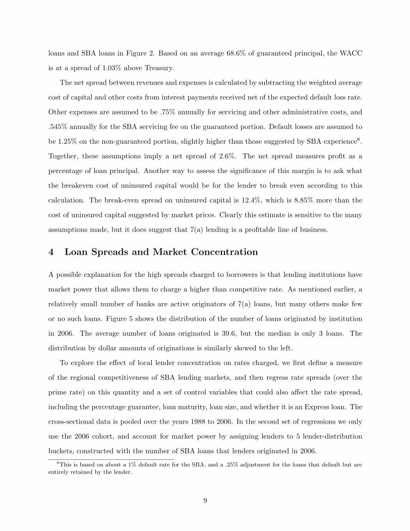
4 Loan Spreads and Market Concentration

A possible explanation for the high spreads charged to borrowers is that lending institutions have

market power that allows them to charge a higher than competitive rate. As mentioned earlier, a

relatively small number of banks are active originators of 7(a) loans, but many others make few

or no such loans. Figure 5 shows the distribution of the number of loans originated by institution

in 2006. The average number of loans originated is 39.6, but the median is only 3 loans. The

distribution by dollar amounts of originations is similarly skewed to the left.

To explore the effect of local lender concentration on rates charged, we first define a measure

of the regional competitiveness of SBA lending markets, and then regress rate spreads (over the

prime rate) on this quantity and a set of control variables that could also affect the rate spread,

including the percentage guarantee, loan maturity, loan size, and whether it is an Express loan. The

cross-sectional data is pooled over the years 1988 to 2006. In the second set of regressions we only

use the 2006 cohort, and account for market power by assigning lenders to 5 lender-distribution

buckets, constructed with the number of SBA loans that lenders originated in 2006.

8This is based on about a 1% default rate for the SBA, and a .25% adjustment for the loans that default but areentirely retained by the lender.

9

For construction of the Herfindahl index, a region is taken to be a Core Based Statistical Area

(CBSA), which defines micropolitan and metropolitan areas. In each of these areas we look at the

level of competition in the lending market for SBA loans. Using the borrower’s zip code we are able

to assign each loan to a CBSA. Then for a given year and a given CBSA we determine the number

and the dollar amount of loans originated by each lender. With this information we calculate a

Herfindahl index for each CBSA and each year. The Herfindahl index for CBSA i at time t is given

by:

H it =

Ni,t∑

n=1

(sin,t

)2, (1)

where sin,t is the market share of lender n, in CBSA i at time t, and Ni,t is the total number

of lenders in CBSA i at time t. The Herfindahl index gives a number between 0 and 1, with 1

representing a monopolistic market and 0 a perfectly competitive market.

The SBA has enacted interest rate-spread limits and maximum loan guarantees based on loan

type, loan size, and maturity. For loans with rates close to the ceiling, this could bias inferences

about the effect of market power on rate spreads. The spread and guarantee limits are presented in

Table 3. In the regressions of spreads on Herfindahl index we split the sample to incorporate these

spreads and guarantee caps, and run a regression for each subsample separately. In the regression

of spread on lender’s distribution we incorporate a dummy variable if the spread of the loan is

within 25 basis point of the interest rate cap.

In table 4 we present the regression results, for tests of spreads on regional concentration. The

sample is subdivided by whether the loan is regular or Express, by loan size, and by maturity.

Control variables include the percentage guaranteed, the loan size, and maturity. All regressions

suggest that the Herfindahl index does not explain higher interest rate spread. In fact, the re-

gressions suggest that regions with more concentrated lending markets are associated with lower

interest rate spreads, which seems counterintuitive. Perhaps borrowers cross city boundaries to

look for affordable loans, and therefore regional concentration may not be the best way to capture

market power. If that is the case, then higher Herfindahl index may be associated with smaller

markets, and perhaps smaller lenders that have less market power. This would be consistent with

the analysis by Petersen and Rajan (2002) [9] who find that in recent years the distance between

10

borrowers and lenders plays a reduced role in relationship lending for small businesses9.

For robustness, we construct an alternative measure of regional banking concentration by relying

on banking activities which are not necessarily related to SBA lending. In particular, we use annual

Summary of Deposits data from the FDIC to estimate the Herfindahl index for each region and

for each calendar year. The FDIC data provides the total deposits of all branches and offices

of all FDIC-insured institutions. For this experiment, a region is taken to be a county, which

covers a broader area than does a CBSA10 . Table 5 displays results for regressions of loan spreads

on regional concentration, using this alternative Herfindahl index. Controls include percentage

guaranteed, loan size, firm size (number of employees), and lagged default rates. The results show

that regional concentration does not explain the high spreads paid by small businesses. The results

are very similar to what was achieved by the regressions using SBA regional concentration.

We consider a size-based measure of lender market power, based on a set of indicator variables for

the number of loans that a lender originated in a given year. The categories are LARGE-LENDERS,

MEDIUM-LENDERS, and SMALL-LENDERS. The SMALL-LENDERS dummy selects the banks

that originated less than the median number of loans. LARGE-LENDERS are alternatively defined

as the top 1st, 5th, or 10th percentile11 . In addition, we introduce a dummy variable to flag Express

loans. To avoid spurious estimation we discard loans that are within 25 basis points of the interest

rate limits shown in table 3.

The results in table 6 suggest that the largest lenders tend to charge higher interest rate spreads

than smaller ones, even after accounting for the lagged default of the lender’s SBA portfolio.

In addition, controlling for other loan characteristics, Express loans charge an extra 127 basis

points above Regular loans. The adjusted-R2 of the current specification shows a slightly higher

explanatory power than the previous specifications. This suggests that some of the unexplained

variation in spreads that was captured by the intercept in previous specifications is accounted for

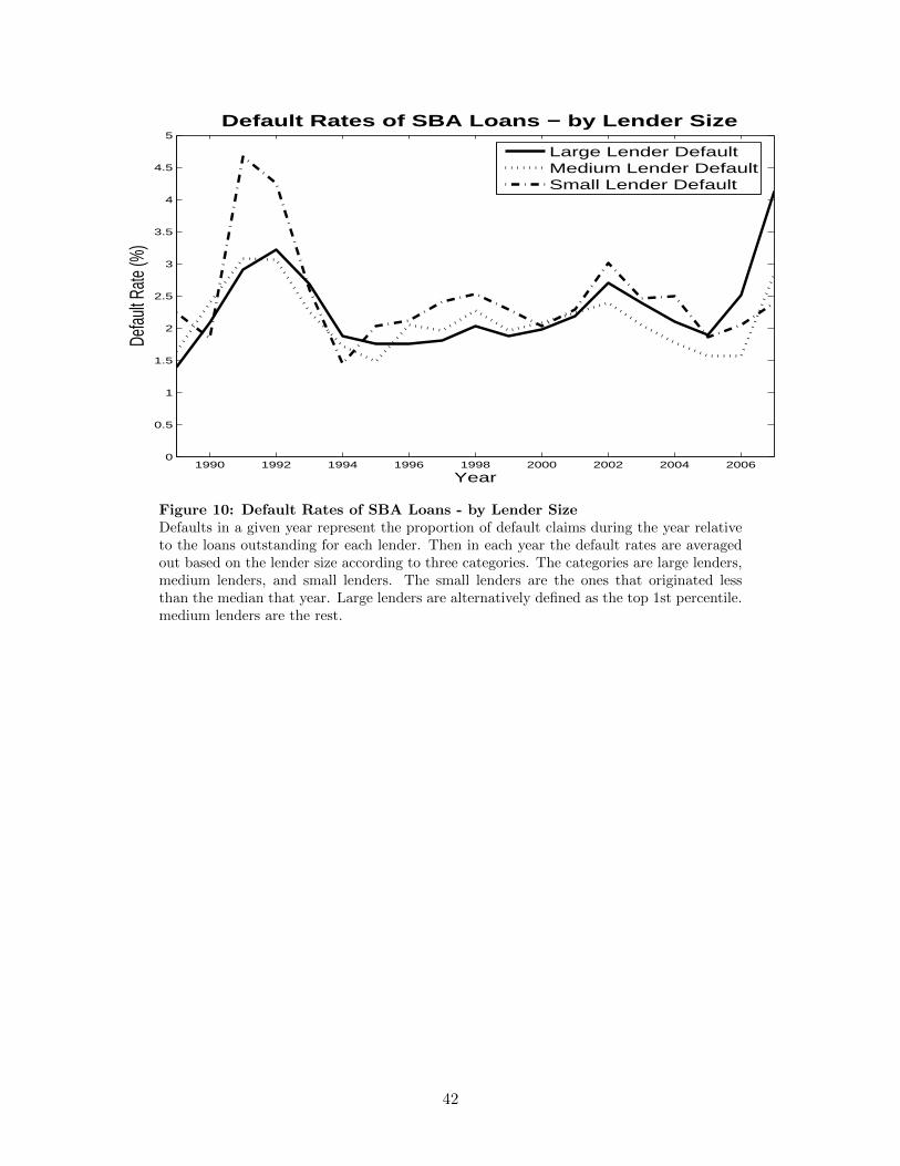
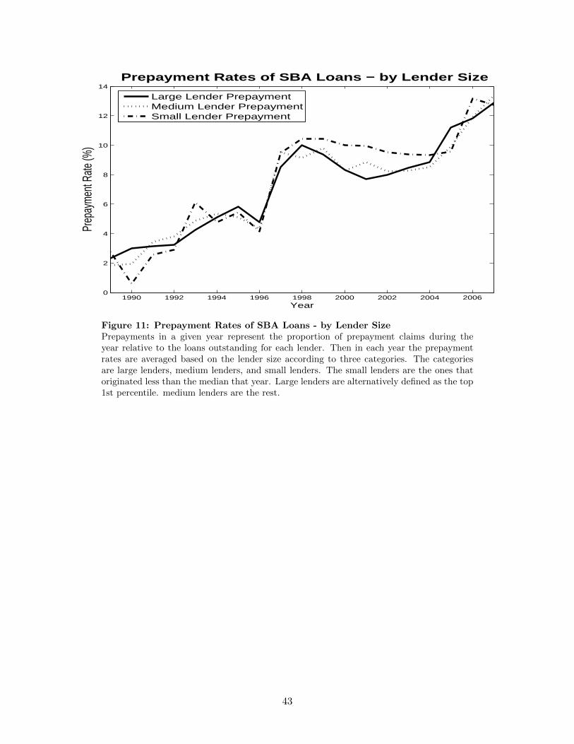
by lenders’ size. Figures 10 and 11 suggest that there are no relevant discrepancies in defaults

and prepayments due to lender size. The only exceptions are the 1991 crisis when small lenders

9Gathering and processing information on small firms is costly, which suggests that long term relationships betweenborrowers and lenders provide a mutual benefit by improving information flow. The reduced importance of distancemay reflect technological advances that have improved the ability to monitor borrower quality from afar.

10Using the FDIC data we also calculate a Herfindahl index based on a CBSA instead of county. The results aresimilar.

11We test different thresholds in our definition of LARGE lenders. As shown on table 5, the results are robust tothe top 1st, 5th, or 10th percentile thresholds.

11

experienced spike in defaults relative to medium and large banks, and in 2007 when large lenders

experienced a higher surge in defaults than small and medium lenders.

An important caveat to this analysis is that it cannot account for the effect of market power

that arises from a lack of sophistication among small business borrowers. To the extent that SBA

borrowers are inclined to take the recommendation of their banker rather than shopping for better

terms, limited competition may exist even in markets with a potentially large number of lenders.

The literature on monopolistic competition suggests that imperfect information leads to imperfect

competition, even in markets with large number of borrowers and lenders. When borrowers face

costly information the market equilibrium is characterized either by lenders charging the monopoly

rate or dispersion of rates above the competitive level (Stiglitz (1979) [11] and Wolinsky (1985)

[14]). A SBA borrower applying for a loan usually does not observe the interest rates offered to

other similar businesses, and therefore can only learn if better terms are available by submitting

loan applications at multiple banks. To the extent that this entails search costs or costly delays in

obtaining funds, such shopping behavior may be limited, leaving borrowers with interest rates that

are above the competitive level.

What remains to be explained is why the largest lenders charge higher interest rates. One

possibility is that large lenders offer a superior product. If large lenders have more branches and

offer a menu of alternative products and services in addition to the loan, they may have an advantage

in attracting small businesses.

5 Cost of Capital for Fully Guaranteed Loans

The analysis thus far suggests that borrowers pay a relatively high rate on SBA loans, and that

the market power of larger lenders may be part of the explanation. We also know, however, that

many banks choose to make very few or no 7(a) loans, suggesting that our estimate of profitability

to lenders in Section 3.2 is likely too high. In this section we show that the apparent profitability

of 7(a) lending is reduced by the fact that the cost of capital for fully guaranteed 7(a) loans is

significantly above Treasury rates, as inferred from the pricing of securities in the Guaranteed Loan

Pool Certificate Program (GLPCP).

12

5.1 Data

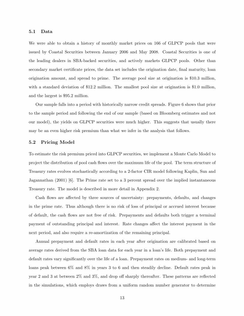
We were able to obtain a history of monthly market prices on 166 of GLPCP pools that were

issued by Coastal Securities between January 2006 and May 2008. Coastal Securities is one of

the leading dealers in SBA-backed securities, and actively markets GLPCP pools. Other than

secondary market certificate prices, the data set includes the origination date, final maturity, loan

origination amount, and spread to prime. The average pool size at origination is $10.3 million,

with a standard deviation of $12.2 million. The smallest pool size at origination is $1.0 million,

and the largest is $95.2 million.

Our sample falls into a period with historically narrow credit spreads. Figure 6 shows that prior

to the sample period and following the end of our sample (based on Bloomberg estimates and not

our model), the yields on GLPCP securities were much higher. This suggests that usually there

may be an even higher risk premium than what we infer in the analysis that follows.

5.2 Pricing Model

To estimate the risk premium priced into GLPCP securities, we implement a Monte Carlo Model to

project the distribution of pool cash flows over the maximum life of the pool. The term structure of

Treasury rates evolves stochastically according to a 2-factor CIR model following Kaplin, Sun and

Jagannathan (2001) [6]. The Prime rate set to a 3 percent spread over the implied instantaneous

Treasury rate. The model is described in more detail in Appendix 2.

Cash flows are affected by three sources of uncertainty: prepayments, defaults, and changes

in the prime rate. Thus although there is no risk of loss of principal or accrued interest because

of default, the cash flows are not free of risk. Prepayments and defaults both trigger a terminal

payment of outstanding principal and interest. Rate changes affect the interest payment in the

next period, and also require a re-amortization of the remaining principal.

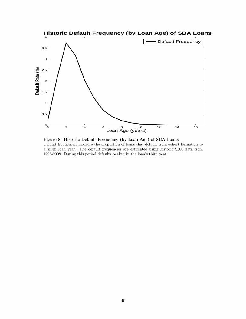
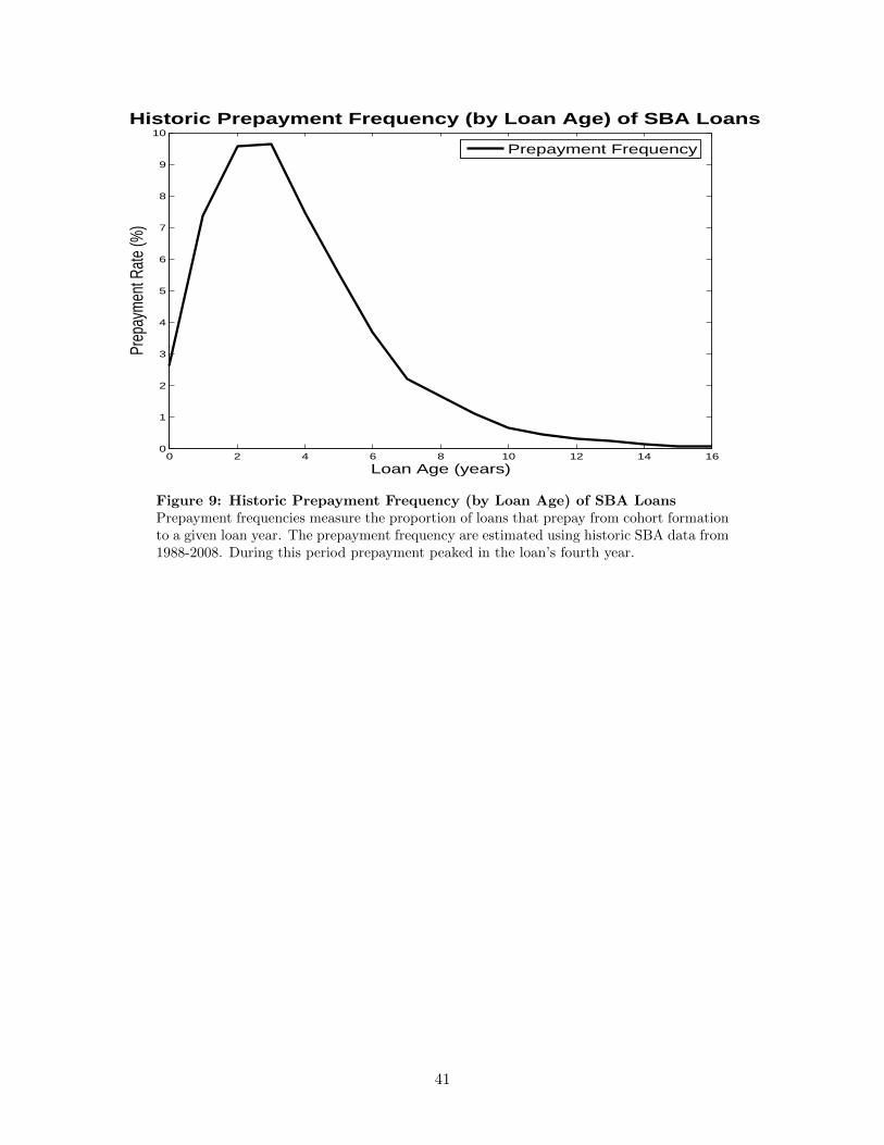
Annual prepayment and default rates in each year after origination are calibrated based on

average rates derived from the SBA loan data for each year in a loan’s life. Both prepayment and

default rates vary significantly over the life of a loan. Prepayment rates on medium- and long-term

loans peak between 6% and 8% in years 3 to 6 and then steadily decline. Default rates peak in

year 2 and 3 at between 2% and 3%, and drop off sharply thereafter. These patterns are reflected

in the simulations, which employs draws from a uniform random number generator to determine

13

whether a default or prepayment has occurred in a given month.

Uncertainty arising from changes in the prime rate, default, and prepayment potentially intro-

duces systematic risk into the cash flows. The spread between Prime and Treasury, which we take

to be fixed, in fact is expected to be countercyclical, since credit spreads increase in downturns.

This imparts a slightly negative beta to the promised cash flows, which thereby get larger when

times are bad. The sign on the systematic risk introduced by default and prepayment is not obvi-

ous. Both trigger an early return of principal, so the effect depends on the systematic risk of the

triggering event, and whether the GLPCP securities tend to systematically priced at a discount

or premium to par in a downturn. Rather than assuming a value for the risk premium, we solve

for the fixed percentage point spread over 1-month Treasury rates implied by the CIR model that

equates the model price with the market price from the Coastal Securities data. The spread can

be interpreted as the sum of a risk premium, a liquidity premium, and an error term due to model

misspecification.

5.3 Results and Sensitivity Analysis

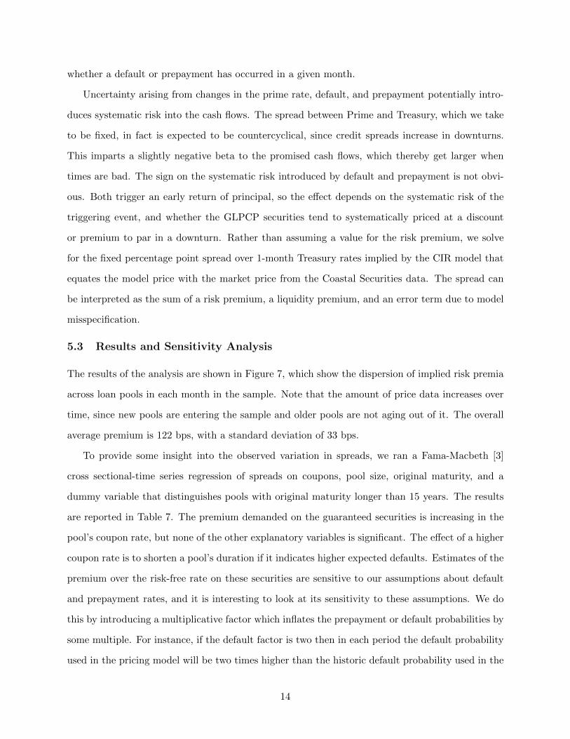
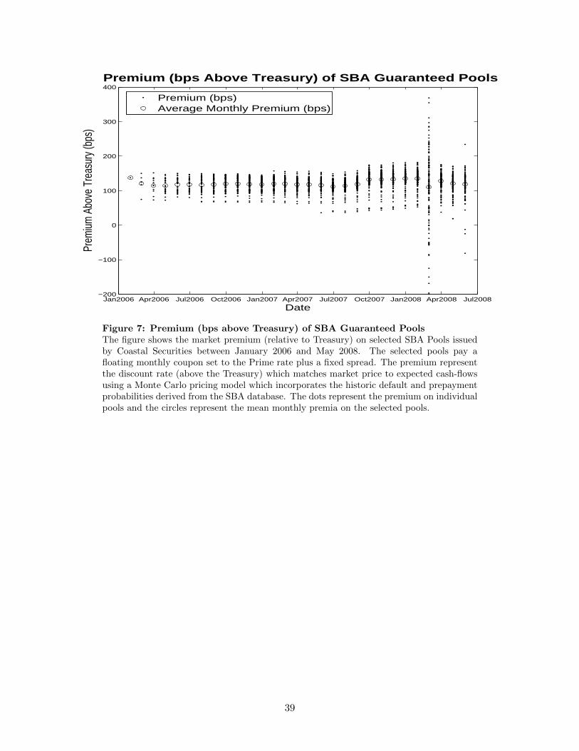
The results of the analysis are shown in Figure 7, which show the dispersion of implied risk premia

across loan pools in each month in the sample. Note that the amount of price data increases over

time, since new pools are entering the sample and older pools are not aging out of it. The overall

average premium is 122 bps, with a standard deviation of 33 bps.

To provide some insight into the observed variation in spreads, we ran a Fama-Macbeth [3]

cross sectional-time series regression of spreads on coupons, pool size, original maturity, and a

dummy variable that distinguishes pools with original maturity longer than 15 years. The results

are reported in Table 7. The premium demanded on the guaranteed securities is increasing in the

pool’s coupon rate, but none of the other explanatory variables is significant. The effect of a higher

coupon rate is to shorten a pool’s duration if it indicates higher expected defaults. Estimates of the

premium over the risk-free rate on these securities are sensitive to our assumptions about default

and prepayment rates, and it is interesting to look at its sensitivity to these assumptions. We do

this by introducing a multiplicative factor which inflates the prepayment or default probabilities by

some multiple. For instance, if the default factor is two then in each period the default probability

used in the pricing model will be two times higher than the historic default probability used in the

14

base case. We find that the default factor which implies a zero premium is on average 21.4 over all

of the loan pools, with a standard deviation of 10.9. This means that in order to match the observed

market prices for a given pool the probability of default in a given month needs to be 21 times

higher than the historical average in the last 20 years. Similarly, the average prepayment factor is

8.0, with a standard deviation of 6.13. This shows that the model prices are quite insensitive to

changes in the default and prepayment probabilities, which also provides a hint that these risks are

not the main drivers of the premium over the risk free rate earned by the guaranteed pools.

5.4 Implications for Profitability

The simple profitability calculation in Section 3.2 took the short-term Treasury rate as the cost of

capital for the guaranteed portion of 7(a) loans. The analysis of this section suggests that the cost is

higher by an average of 127 bps. Taking this into account in the cost of capital calculation decreases

estimated profits as a percent of loan value from 2.6% to 1.6%, and decreases the breakeven cost

of uninsured capital from 17.6% to 14.3%. Hence, the significantly higher than risk-free cost of

capital to finance the guaranteed portion of SBA 7(a) loans explains part, but not all, of why loans

cost borrowers so much.

6 Summary and Conclusions

In this paper we have looked at two possible and complementary explanations for the high rates

charged to borrowers in the 7(a) program. We find support in the data for both: (1) that large

SBA lenders may be able to exert market power and thereby charge higher rates, and (2) that

the cost of funding the guaranteed portion of SBA loans is significantly above Treasury’s cost of

funds. These findings suggest that there may be ways to modify the 7(a) program to reduce costs

to borrowers and finance the program more efficiently.

The leading alternative to guaranteed lending is direct lending, where the government directly

funds and originates loans. A rationale for involving private intermediaries in the origination pro-

cess for government loan programs is when screening for credit quality is important. Although

we did not try to assess the value of this function for the 7(a) program, clearly small business

loans are risky and require judgment, suggesting an important screening role for the private sector.

Nevertheless, it seems that the government could reduce program costs by purchasing the guaran-

15

teed portion of loans directly from bank lenders and funding those purchases through the Treasury

rather than through sponsorship of a private securitized loan market 12. This would allow bank

lenders to continue to provide screening services in the origination process, but eliminate a layer

of intermediation in the securitization process where there is no obvious value added by operating

through the private sector.

If in fact large SBA lenders are able to exert market power in loan pricing, a further role

for the federal government could be to try to increase competitiveness in the market, perhaps

by introducing a more centralized loan application process that would force lenders to compete

more directly for borrowers. This would be consistent with the general trend toward the increased

reliance on credit scoring and other types of hard information in small business lending, although

local lenders may still have information advantages that make them the most efficient originators.

12This was the rationale in 1973 for consolidating federal borrowing for different programs through the FederalFinancing Bank.

16

A APPENDIX - SBA 7(a) Loan Level Data

The SBA administers 7(a) Program data in their Electronic Loan Information Processing System

(ELIPS). This system incorporates static data – information that does not regularly change over

the life of a loan – as well as loan transactions related to balance, purchase, recovery, and other

activities. The current project relies on data from ELIPS to identify basic loan, size, maturity,

lender information, borrower zip code, as well as transactions data to track loan performance

related to purchases and recoveries to identify defaults and prepayments.

Static Loans File: The ELIPS file consists of over 1.2m of SBA loans since the program has

been in place, with one static record per loan. Each record contains a list of relevant information

introduced at time of origination. It includes record of the following: date the loan was issued,

loan amount, loan size, maturity date, SBA guarantee, interest rate (including the spread above

prime rate), program type (Regular or Express), borrower and lender’s zip code, lender’s name,

and characteristics of the business.

Transactions File: The file consists of all transactions for each corresponding loan in the static

file. These transactions include disbursements, monthly loan payments (including fees), balance,

SBA loan repurchases when there is default, and recoveries (given default). Based on the infor-

mation contained in the transaction file it is possible to determine whether and when default and

prepayment have occurred. The transactions file also provides full information about recoveries

and other information which are important in determining the default and prepayment behavior of

all SBA loans.

17

B APPENDIX - Valuing GLPCP Securities (SBA Pools)

B.1 Overview of Securities and Underlying Risks

The GLPCP securities (SBA pools) in our dataset amortize every month and pays interest at

PRIME rate plus a fixed spread. The pool cash flows are subject to early termination in the form

of default or prepayment. Either of these events triggers a final payment of outstanding principal

and accrued interest. There is full and explicit Government guarantee on these securities, which

means that certificate holders do not lose any principal when default occurs. However, since these

pools typically trade above par, when these pools terminate earlier than expected investors may

lose the difference between the market price and the remaining principal plus accrued interest.

Yet, it is unclear which portion of these risks is diversifiable and which portion is systematic. The

approach used to address this question is to treat these risks as independent from interest rate risk,

and use the historic default and prepayment to model these events. Furthermore, we perform a

sensitivity analysis to infer that the magnitude of an increase in default (prepayment) frequency

does not have a large impact on pool prices.

This appendix describes details of the Monte Carlo implementation used to model the distribu-

tion of pool cash flows and the value of the certificates, and is organized as follows; we first use a

two-factor Cox-Ingersoll-Ross (CIR) model to simulate risk-neutral paths of interest rates used for

credit-risk-free discounting and for determining the pool floating interest payments. We then model

prepayment and default using the historic experience derived from 20 years of comprehensive data

obtained from the SBA. We combine these three components to compute the value of each pool in

our sample, and then devise an algorithm to measure the spread above Treasuries embedded in the

market price of these securities.

B.2 Interest Rates and Pool Amortization

We employ a two-factor CIR model to simulate paths of future Treasury rates. In the Jagannathan

Kaplin Sun (JKS – 2003) [6] version of the CIR model the instantaneous interest rate R (t) is the

sum of a constant R and the two state variables yi (t), for i = 1, 2:

R (t) = R+ y1 (t) + y2 (t) . (2)

Each state variable follows an independent, mean-reverting, square root process along any period

18

s, between time t and the maturity date T :

dyi (s) = ·i [µi − yi (s)] ds+ ¾i√

yi (s)dWi (s) , i = 1, 2 (3)

where Wi (s) are standard and independent Brownian motions. Under the pricing (risk-neutral)

measure the factors evolve according to:

dyi (s) = ·i[µi − yi (s)

]ds+ ¾i

√yi (s)dW

∗i (s) , i = 1, 2 (4)

where

·i = ·i + ¸i (5)

and

µi =·iµi

·i + ¸i(6)

The market price of risk, ¸i for each state variable is assumed to be linear. The price at

current-time t of a zero coupon bond that pays $1 at maturity date T is

P (t, T ) = e−R(T−t)p1 (t, T ) p2 (t, T ) , (7)

where

pi (t, T ) = eAi(t,T )−B(t,T )yi(t), (8)

Ai (t, T ) =2·iµi¾2i

ln

⎡⎣ 2°i exp

{(°i + ·i)

(T−t)2

}

2°i + (°i + ·i) [exp {°i(T − t)} − 1]

⎤⎦ , (9)

Bi (t, T ) =2 (exp [°i(T − t)]− 1)

2°i + (°i + ·i) [exp {°i(T − t)} − 1], (10)

and

°i =√

·2i + 2¾2i (11)

The yield to maturity, Y TM of a zero coupon bond maturing at T is

Y TM (t, T ) =− lnP (t, T )

T − t(12)

In our analysis we use the two-factor parameters estimated in JKS [6] using weekly LIBOR

rates of various maturities:

19

Two factor CIR parameters (estimated by JKS)

Factor · µ ¾ ¸1 0.3922 0.2727 0.0153 -0.000382 0.0532 0.0162 0.0430 -0.05917

R = −0.2289

Factor 1 has stronger degree of mean reversion and drives the gap between long and short rates.

Factor 2 has higher volatility parameter.

In every period t we solve for the initial state variables, y1(t) and y2(t), by fitting two points in

the yield curve from historic Treasury data, the three month T-Bill rate and the ten year Treasury

bond rate. We perform this in two steps, first set the historic yields on left hand side of equation

(12) to solve for P (t, T ). Then use P and system (7) – (11) to solve for y1(t) and y2(t).

We need initial state variables to simulate the (monthly) discrete version of (4), with Monte

Carlo paths that start at time t and end at T . Using monthly Euler-discretizations we set time

step ℎ = 112 . For any time s between t and T we have:

yi (s+ ℎ) = yi (s) + ·i[µi − yi (s)

]ℎ+ ¾i

√max {yi (s) , 0}

√ℎWi (13)

where W ’s are drawn from standard and independent normal random generator.

From (2) and the initial state variables we compute the initial short rate R(t). In turn, cash

flows arriving t+ ℎ are discounted back to t using the factor

d (t, t+ ℎ) =1

1 +R (t)ℎ(14)

Cash flows arriving at s + ℎ are discounted back to t using a factor which can be recursively

solved from (14)

d (t, s+ ℎ) =s∏

u=t

d(u, u+ ℎ) (15)

=d (t, s)

1 +R (s)ℎ

We assume that the prime rate is 3% above the short rate13. Suppose a SBA guaranteed pool

pays the fixed spread above prime, Δ. Then for the same Monte Carlo run as above we set the

pool’s floating interest rate to

½ (s) = R (s) + 0.03 + Δ (16)

13Figure 1 indicates that after 1994 the Prime rate has been consistently set to 300 basis points above the FedFunds rate plus a very small noise. In addition, the Fed Funds rate has usually been higher than the short rate.

20

For a given balance B(s) the pool payment in the next month (when there is no termination)

and new balance are set by the amortization schedule:

Pmt (s+ ℎ) =B (s) ½(s)ℎ

1− (1 + ½(s)ℎ)s−(T−t)(17)

and

B (s+ ℎ) = [1 + ½(s)ℎ]B (s)− Pmt (s+ ℎ) . (18)

B.3 Default and Prepayment

A guaranteed pool is formed with the insured portion of several14 SBA loans. In practice these

certificates may experience partial termination when only some, and not all of the underlying loans

default or prepay. Instead of buying a pool certificate investors could acquire a single guaranteed

loan certificate, which would be a claim on the insured portion of a single SBA loan. A large pool

does not diversify away the systematic risk and therefore must be priced in the same way as a single

guaranteed loan certificate. Hence, for valuation purposes we can model pools as if they were single

loans by assuming that default or prepayment triggers full termination. The termination events

in this section are reflected in simulations, which employ draws from a uniform random number

generator to determine whether a loan has defaulted or prepaid.

We estimate default and prepayment frequencies as a function of loan age, using twenty years

of comprehensive data provided by the SBA. The historic prepayment and default frequencies are

summarized in figures 8 and 9. From those frequencies we can easily calculate the contemporenous

default and prepayment probabilities. In period s the default and prepayment probabilities for loan

j are expressed by ¼dj (s) and ¼p

j (s), respectively.

In time step s of the Monte Carlo run we draw W to feed in the expression of eq. (13) and

we also draw two independent numbers from a uniform number generator, Uds and Up

s . Default on

loan j is triggered if Uds ≤ ¼d

j (s) and prepayment is triggered if Ups ≤ ¼p

j (s). When either event

occurs the pool terminates and investors receive the remaining balance plus any accrued interest.

In those nodes Pmt in (17) becomes:

Pmt (s) = [1 + ½ (s− ℎ)ℎ]B (s− ℎ) (19)

14A pool must be issued with at least four underlying loans. The pool holds only the guaranteed portion of theloans. This means that the uninsured piece would have been stripped out before the pool has been assembled.

21

For valuation purposes it is convenient to set Pmt (u) = 0 for any u > s, where s is a termination

time.

B.4 Model Price

Using the interest rate behavior and termination behavior above we obtain pool prices at any time

t. The only inputs for each pool are the origination date to, the maturity date T , and the pool’s

fixed spread above the prime rate Δ. For a given Monte Carlo path indexed by n the price at time

t of the pool j is

mnj (t) =

T∑

s=t+1

Pmt(s)d(t, s) (20)

The model price of pool j at time t is computed as the average price of all simulated paths, and

represented by

Mj (t) =1

N

N∑

n=1

mnj (t) (21)

In our simulations we set the number of sample paths to N = 100, 000.

B.5 Market Prices, Spreads, and Sensitivity

In our sample, pool market prices are often lower than model prices Mj(t), which suggests that

investors discount pool cash flows at higher than (credit-risk-free) Treasury rates. Alternatively,

investors may demand a premium for bearing any systematic termination-risk which may not

have been accounted in our model. In this section we introduce a premium above (or below) the

Treasury curve which equates model prices to market prices. We also perform a similar exercise

by introducing a multiplicative premium over default and prepayment probabilities to examine the

price impact of changes in termination probabilities.

Define the discount premium ³, and add it to the factor (14) to discount cash flows from t+ ℎ

back to t and (15) to discount cash flows from s + ℎ back to t. For s > t we rewrite the discount

factors to incorporate premium ³ as:

d (³; t, t+ ℎ) =1

1 + [R (t) + ³]ℎ(22)

and

d (³; t, s+ ℎ) =s∏

u=t

d(³;u, u+ ℎ) (23)

22

=d (Ã; t, s)

1 + [R (s) + ³]ℎ

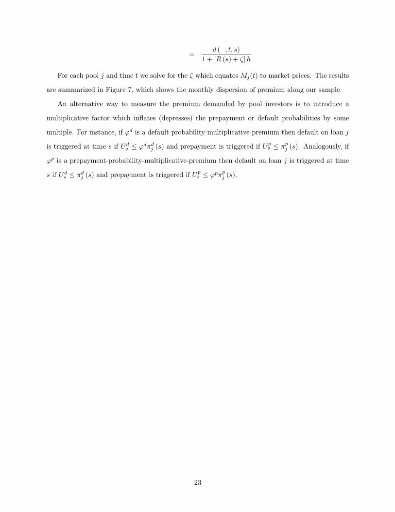
For each pool j and time t we solve for the ³ which equates Mj(t) to market prices. The results

are summarized in Figure 7, which shows the monthly dispersion of premium along our sample.

An alternative way to measure the premium demanded by pool investors is to introduce a

multiplicative factor which inflates (depresses) the prepayment or default probabilities by some

multiple. For instance, if 'd is a default-probability-multiplicative-premium then default on loan j

is triggered at time s if Uds ≤ 'd¼d

j (s) and prepayment is triggered if Ups ≤ ¼p

j (s). Analogously, if

'p is a prepayment-probability-multiplicative-premium then default on loan j is triggered at time

s if Uds ≤ ¼d

j (s) and prepayment is triggered if Ups ≤ 'p¼p

j (s).

23

References

[1] Collin-Dufresne, Pierre and Bruno Solnik (2001), “On the Term Structure of Default Premia

in the Swap and LIBOR Markets,” Journal of Finance 56, 1095-1115

[2] Cox, J. C., J. E. Ingersoll and S. A. Ross (1985), “A Theory of the Term Structure of Interest

Rates,” Econometrica, vol. 53, pp. 385-408.

[3] Fama,Eugene F. and James D. MacBeth, “Risk, Return, and Equilibrium: Empirical Tests ”

The Journal of Political Economy, Vol. 81, No. 3 (May - Jun., 1973), pp. 607-636

[4] Gale, W.G. (1991), “Economic Effects of Federal Credit Programs,” The American Economic

Review, vol. 81, no. 1, pp. 133-152.

[5] Glennon, D. and P. Nigro (2005), “Measuring the Default Risk of Small Business Loans: A

Survival Analysis Approach,” Journal of Money, Credit, and Banking, vol. 37, no. 5.

[6] Jagannathan, R., A. Kaplin, and S.G. Sun, (2003), “An Evaluation of Multi-Factor CIR Models

Using LIBOR, Swap Rates, and Cap and Swaption Prices,” Journal of Econometrics, vol.

116(1-2), pp. 113-146.

[7] Longstaff, F. (2004), “The Flight-to-Liquidity Premium in U.S. Treasury Bond Prices,” The

Journal of Business, 2004, vol. 77, no. 3.

[8] Lucas, D. and Damien Moore (2009), “Guaranteed vs. Direct Lending: The Case of Student

Loans,” forthcoming in Measuring and Managing Federal Financial Risk, D. Lucas editor,

NBER.

[9] Petersen, M. and R.G. Rajan (2002) “Does Distance Still Matter? The Information Revolution

in Small Business Lending”, Journal of Finance, 57 (6): 2533-2570 Dec 2002.

[10] SBA (2007), “The Small Business Economy for Data Year 2006,” US Government Printing

Office, http://www.sba.gov/advo/research/sb econ2007.pdf

[11] Stiglitz, J. E. (1979) “Equilibrium in Product Markets with Imperfect Information”, The

American Economic Review, Vol. 69, No. 2, Papers and Proceedings of the Ninety-First Annual

Meeting of the American Economic Association (May, 1979), pp. 339-345.

24

[12] U.S. Congressional Budget Office (2005), “Estimating the Value of Subsidies for Federal Loans

and Guarantees,” Washington, D.C.

[13] U.S. Congressional Budget Office (2007), “Federal Financial Guarantees under the Small

Business Administration’s 7(a) Program,” http://www.cbo.gov/ftpdocs/87xx/doc8708/10-15-

SBA.pdf

[14] Wolinsky, Asher (1986) “True Monopolistic Competition as a Result of Imperfect Information”,

The Quarterly Journal of Economics, Vol. 101, No. 3 (Aug., 1986), pp. 493-511.

25

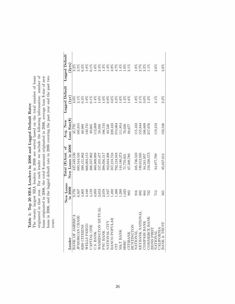
Table

1:Top

20SBA

Lenders

in2006and

Lagged

Default

Rates

Thetw

enty

largestSBA

lendersin

2006

aresorted

based

onthetotalnumber

ofloan

soriginatedin

that

year.

For

each

lender

weincludethefollow

inginform

ation

:number

ofloansoriginated

in2006,thetotal$-am

ountoriginated

in2006,averageloan

$-size

ofnew

loansin

2006,an

dthelagged

defau

ltrate

in2006

coveringthepastyearandthepast

two

years.

Lender

New

Loans

in2006

Tota

l($

)Amt.

of

New

Loansin

2006

Avg.New

Loan

Size($

)

Lagged

Default

(1yr)

Lagged

Default

(2yrs)

BANK

OF

AMERIC

A9,776

447,449,130

45,770

4.0%

3.2%

JPMORGAN

CHASE

6,567

695,544,516

105,915

2.1%

2.5%

RBSCIT

IZENS

4,905

299,151,862

60,989

0.3%

0.2%

WELLSFARGO

4,448

666,003,115

149,731

1.9%

1.8%

CAPIT

ALONE

4,159

206,557,962

49,665

0.1%

0.1%

U.S.BANK

4,093

460,909,009

112,609

1.4%

1.6%

WASHIN

GTON

MUTUAL

2,653

157,455,477

59,350

1.0%

2.4%

PNC

BANK

2,078

388,056,517

186,745

1.0%

1.3%

NATIO

NALCIT

Y1,947

162,624,308

83,526

0.9%

1.3%

BANCO

POPULAR

1,492

357,218,724

239,423

3.6%

3.9%

CIT

1,380

792,124,943

574,004

4.2%

4.7%

M&T

BANK

1,289

144,180,273

111,854

1.6%

1.4%

HSBC

1,025

71,770,931

70,020

1.2%

1.0%

CIT

IBANK

983

67,509,780

68,677

1.6%

2.1%

HUNTIN

GTON

NATIO

NAL

916

105,736,523

115,433

1.8%

1.8%

KEYBANK

NATIO

NAL

892

139,012,935

155,844

2.1%

2.7%

COMPASSBANK

884

94,241,957

106,609

3.0%

3.2%

COMMERCE

BANK

732

159,338,573

217,676

1.2%

1.1%

ZIO

NSFIR

ST

NATIO

NAL

712

84,877,789

119,210

2.1%

2.6%

CALIF

ORNIA

BANK

&TRUST

565

85,047,012

150,526

2.2%

2.0%

26

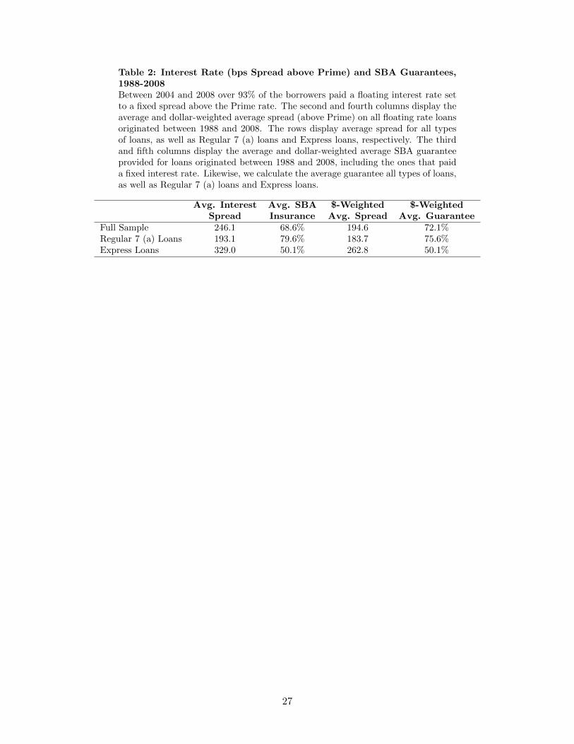
Table 2: Interest Rate (bps Spread above Prime) and SBA Guarantees,1988-2008Between 2004 and 2008 over 93% of the borrowers paid a floating interest rate setto a fixed spread above the Prime rate. The second and fourth columns display theaverage and dollar-weighted average spread (above Prime) on all floating rate loansoriginated between 1988 and 2008. The rows display average spread for all typesof loans, as well as Regular 7 (a) loans and Express loans, respectively. The thirdand fifth columns display the average and dollar-weighted average SBA guaranteeprovided for loans originated between 1988 and 2008, including the ones that paida fixed interest rate. Likewise, we calculate the average guarantee all types of loans,as well as Regular 7 (a) loans and Express loans.

Avg. InterestSpread

Avg. SBAInsurance

$-WeightedAvg. Spread

$-WeightedAvg. Guarantee

Full Sample 246.1 68.6% 194.6 72.1%Regular 7 (a) Loans 193.1 79.6% 183.7 75.6%Express Loans 329.0 50.1% 262.8 50.1%

27

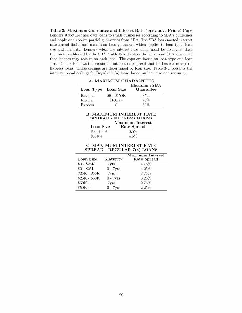
Table 3: Maximum Guarantee and Interest Rate (bps above Prime) CapsLenders structure their own loans to small businesses according to SBA’s guidelinesand apply and receive partial guarantees from SBA. The SBA has enacted interestrate-spread limits and maximum loan guarantee which applies to loan type, loansize and maturity. Lenders select the interest rate which must be no higher thanthe limit established by the SBA. Table 3-A displays the maximum SBA guaranteethat lenders may receive on each loan. The caps are based on loan type and loansize. Table 3-B shows the maximum interest rate spread that lenders can charge onExpress loans. These ceilings are determined by loan size. Table 3-C presents theinterest spread ceilings for Regular 7 (a) loans based on loan size and maturity.

A. MAXIMUM GUARANTEES

Loan Type Loan SizeMaximum SBA

Guarantee

Regular $0 - $150K 85%Regular $150K+ 75%Express all 50%

B. MAXIMUM INTEREST RATESPREAD - EXPRESS LOANS

Loan SizeMaximum Interest

Rate Spread$0 - $50K 6.5%$50K+ 4.5%

C. MAXIMUM INTEREST RATESPREAD - REGULAR 7(a) LOANS

Loan Size MaturityMaximum Interest

Rate Spread$0 - $25K 7yrs + 4.75%$0 - $25K 0 - 7yrs 4.25%$25K - $50K 7yrs + 3.75%$25K - $50K 0 - 7yrs 3.25%$50K + 7yrs + 2.75%$50K + 0 - 7yrs 2.25%

28

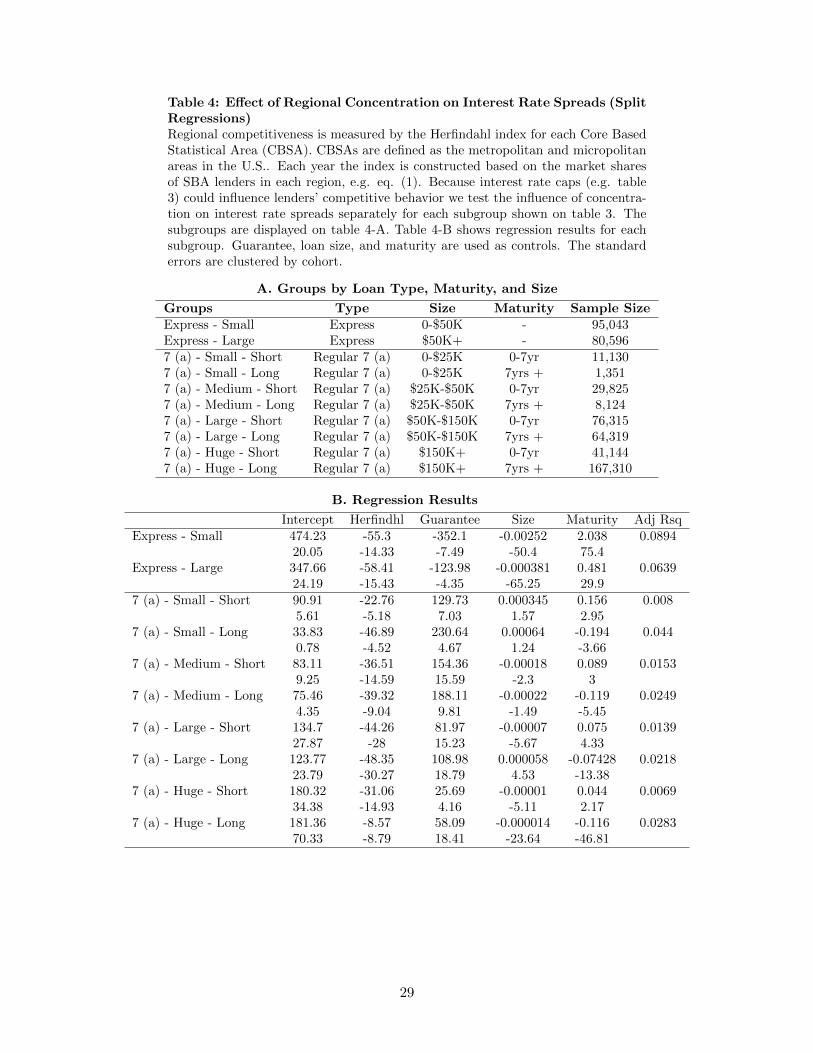
Table 4: Effect of Regional Concentration on Interest Rate Spreads (SplitRegressions)Regional competitiveness is measured by the Herfindahl index for each Core BasedStatistical Area (CBSA). CBSAs are defined as the metropolitan and micropolitanareas in the U.S.. Each year the index is constructed based on the market sharesof SBA lenders in each region, e.g. eq. (1). Because interest rate caps (e.g. table3) could influence lenders’ competitive behavior we test the influence of concentra-tion on interest rate spreads separately for each subgroup shown on table 3. Thesubgroups are displayed on table 4-A. Table 4-B shows regression results for eachsubgroup. Guarantee, loan size, and maturity are used as controls. The standarderrors are clustered by cohort.

A. Groups by Loan Type, Maturity, and Size

Groups Type Size Maturity Sample SizeExpress - Small Express 0-$50K - 95,043Express - Large Express $50K+ - 80,5967 (a) - Small - Short Regular 7 (a) 0-$25K 0-7yr 11,1307 (a) - Small - Long Regular 7 (a) 0-$25K 7yrs + 1,3517 (a) - Medium - Short Regular 7 (a) $25K-$50K 0-7yr 29,8257 (a) - Medium - Long Regular 7 (a) $25K-$50K 7yrs + 8,1247 (a) - Large - Short Regular 7 (a) $50K-$150K 0-7yr 76,3157 (a) - Large - Long Regular 7 (a) $50K-$150K 7yrs + 64,3197 (a) - Huge - Short Regular 7 (a) $150K+ 0-7yr 41,1447 (a) - Huge - Long Regular 7 (a) $150K+ 7yrs + 167,310

B. Regression Results

Intercept Herfindhl Guarantee Size Maturity Adj RsqExpress - Small 474.23 -55.3 -352.1 -0.00252 2.038 0.0894

20.05 -14.33 -7.49 -50.4 75.4Express - Large 347.66 -58.41 -123.98 -0.000381 0.481 0.0639

24.19 -15.43 -4.35 -65.25 29.97 (a) - Small - Short 90.91 -22.76 129.73 0.000345 0.156 0.008

5.61 -5.18 7.03 1.57 2.957 (a) - Small - Long 33.83 -46.89 230.64 0.00064 -0.194 0.044

0.78 -4.52 4.67 1.24 -3.667 (a) - Medium - Short 83.11 -36.51 154.36 -0.00018 0.089 0.0153

9.25 -14.59 15.59 -2.3 37 (a) - Medium - Long 75.46 -39.32 188.11 -0.00022 -0.119 0.0249

4.35 -9.04 9.81 -1.49 -5.457 (a) - Large - Short 134.7 -44.26 81.97 -0.00007 0.075 0.0139

27.87 -28 15.23 -5.67 4.337 (a) - Large - Long 123.77 -48.35 108.98 0.000058 -0.07428 0.0218

23.79 -30.27 18.79 4.53 -13.387 (a) - Huge - Short 180.32 -31.06 25.69 -0.00001 0.044 0.0069

34.38 -14.93 4.16 -5.11 2.177 (a) - Huge - Long 181.36 -8.57 58.09 -0.000014 -0.116 0.0283

70.33 -8.79 18.41 -23.64 -46.81

29

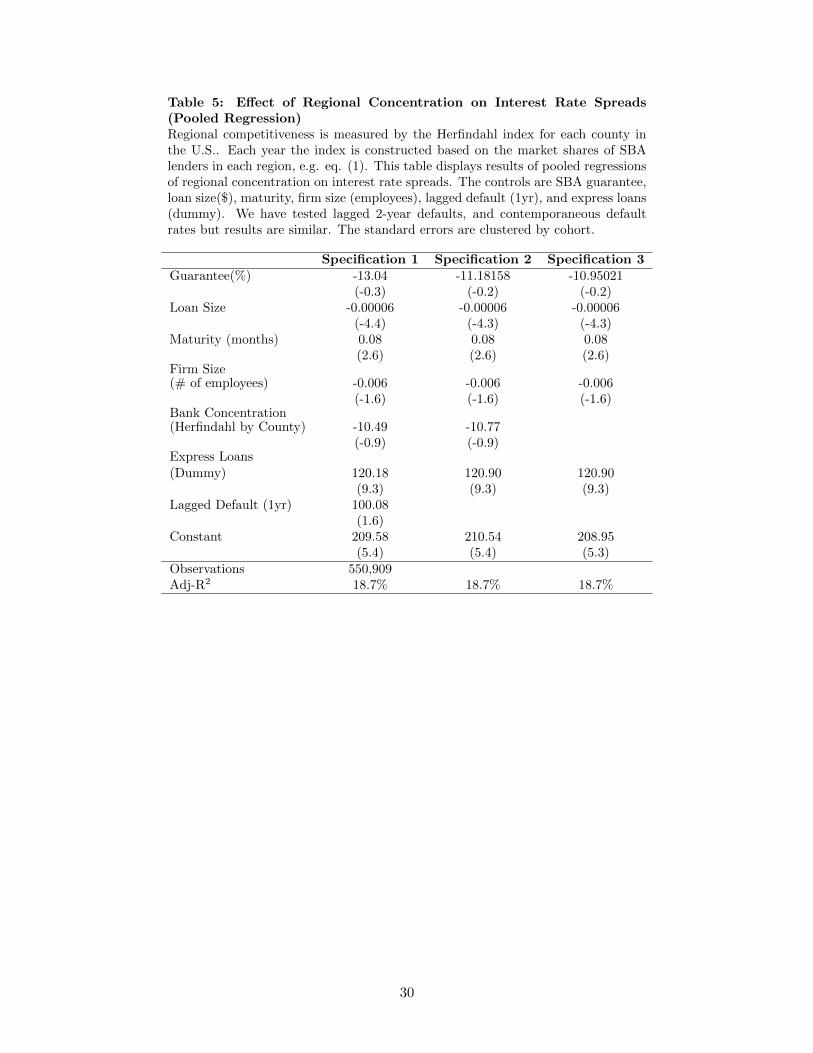
Table 5: Effect of Regional Concentration on Interest Rate Spreads(Pooled Regression)Regional competitiveness is measured by the Herfindahl index for each county inthe U.S.. Each year the index is constructed based on the market shares of SBAlenders in each region, e.g. eq. (1). This table displays results of pooled regressionsof regional concentration on interest rate spreads. The controls are SBA guarantee,loan size($), maturity, firm size (employees), lagged default (1yr), and express loans(dummy). We have tested lagged 2-year defaults, and contemporaneous defaultrates but results are similar. The standard errors are clustered by cohort.

Specification 1 Specification 2 Specification 3Guarantee(%) -13.04 -11.18158 -10.95021

(-0.3) (-0.2) (-0.2)Loan Size -0.00006 -0.00006 -0.00006

(-4.4) (-4.3) (-4.3)Maturity (months) 0.08 0.08 0.08

(2.6) (2.6) (2.6)Firm Size(# of employees) -0.006 -0.006 -0.006

(-1.6) (-1.6) (-1.6)Bank Concentration(Herfindahl by County) -10.49 -10.77

(-0.9) (-0.9)Express Loans(Dummy) 120.18 120.90 120.90

(9.3) (9.3) (9.3)Lagged Default (1yr) 100.08

(1.6)Constant 209.58 210.54 208.95

(5.4) (5.4) (5.3)Observations 550,909Adj-R2 18.7% 18.7% 18.7%

30

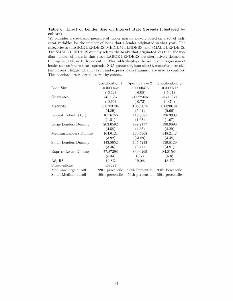
Table 6: Effect of Lender Size on Interest Rate Spreads (clustered bycohort)We consider a size-based measure of lender market power, based on a set of indi-cator variables for the number of loans that a lender originated in that year. Thecategories are LARGE-LENDERS, MEDIUM-LENDERS, and SMALL-LENDERS.The SMALL LENDERS dummy selects the banks that originated less than the me-dian number of loans in that year. LARGE LENDERS are alternatively defined asthe top 1st, 5th, or 10th percentile. This table displays the result of a regression oflender size on interest rate spreads. SBA guarantee, loan size($), maturity, firm size(employees), lagged default (1yr), and express loans (dummy) are used as controls.The standard errors are clustered by cohort.

Specification 1 Specification 2 Specification 3Loan Size -0.0000446 -0.0000476 -0.0000477

(-6.32) (-6.08) (-5.91)Guarantee -37.7587 -41.22346 -46.15977

(-0.66) (-0.72) (-0.79)Maturity 0.0783794 0.0830075 0.0890191

(4.89) (5.61) (5.66)Lagged Default (1yr) 107.6756 119.0581 126.3903

(1.51) (1.63) (1.67)Large Lenders Dummy 203.0592 192.2177 190.9896

(4.58) (4.35) (4.29)Medium Lenders Dummy 164.6121 160.4368 148.2142

(3.92) (-3.89) (3.48)Small Lenders Dummy 143.8052 145.5233 159.8129

(3.46) (3.47) (3.81)Express Loans Dummy 77.87298 83.09269 84.81583

(5.34) (5.7) (5.8)Adj-R2 19.8% 19.0% 18.7%Observations 459523Medium-Large cutoff 99th percentile 95th Percentile 90th PercentileSmall-Medium cutoff 50th percentile 50th percentile 50th percentile

31

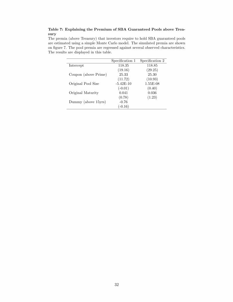
Table 7: Explaining the Premium of SBA Guaranteed Pools above Trea-suryThe premia (above Treasury) that investors require to hold SBA guaranteed poolsare estimated using a simple Monte Carlo model. The simulated premia are shownon figure 7. The pool premia are regressed against several observed characteristics.The results are displayed in this table.

Specification 1 Specification 2Intercept 118.35 118.85

(19.16) (29.25)Coupon (above Prime) 25.33 25.30

(11.72) (10.93)Original Pool Size -5.42E-10 1.55E-08

(-0.01) (0.40)Original Maturity 0.041 0.036

(0.78) (1.23)Dummy (above 15yrs) -0.76

(-0.16)

32

Jan1990 Jul1992 Jan1995 Jul1997 Jan2000 Jul2002 Jan2005 Jul20070

2

4

6

8

10

12

Date

Annu

alize

d Per

centa

ge Historic PRIME, Fed Funds, and (1yr)T−Bills Rates

Prime RateFed Funds (target)1yr T−Bill

Figure 1: Historic PRIME, Fed Funds, and (1yr) T-Bill RatesThe figure shows the evolution of the Prime rate, Fed Funds (effective) rate, and the 1 yearT-Bill rate. Since the end of 1994 the difference between the Prime rate and the Fed Funds(effective) rate have hovered around 3%.

33

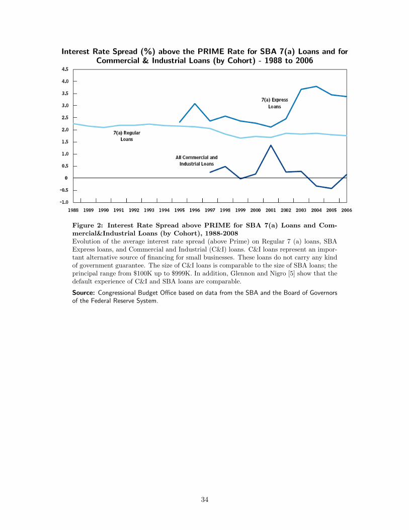
Interest Rate Spread (%) above the PRIME Rate for SBA 7(a) Loans and forCommercial & Industrial Loans (by Cohort) - 1988 to 2006

Figure 2: Interest Rate Spread above PRIME for SBA 7(a) Loans and Com-mercial&Industrial Loans (by Cohort), 1988-2008Evolution of the average interest rate spread (above Prime) on Regular 7 (a) loans, SBAExpress loans, and Commercial and Industrial (C&I) loans. C&I loans represent an impor-tant alternative source of financing for small businesses. These loans do not carry any kindof government guarantee. The size of C&I loans is comparable to the size of SBA loans; theprincipal range from $100K up to $999K. In addition, Glennon and Nigro [5] show that thedefault experience of C&I and SBA loans are comparable.

Source: Congressional Budget Office based on data from the SBA and the Board of Governorsof the Federal Reserve System.

34

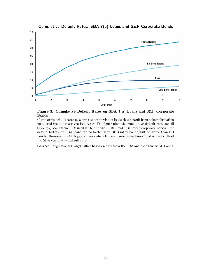
Cumulative Default Rates: SBA 7(a) Loans and S&P Corporate Bonds

Figure 3: Cumulative Default Rates on SBA 7(a) Loans and S&P CorporateBondsCumulative default rates measure the proportion of loans that default from cohort formationup to and including a given loan year. The figure plots the cumulative default rates for allSBA 7(a) loans from 1988 until 2006, and the B, BB, and BBB-rated corporate bonds. Thedefault history on SBA loans are no better than BBB-rated bonds, but no worse than BBbonds. However, the SBA guarantees reduce lenders’ cumulative losses to about a fourth ofthe SBA cumulative default rate.

Source: Congressional Budget Office based on data from the SBA and the Standard & Poor’s.

35

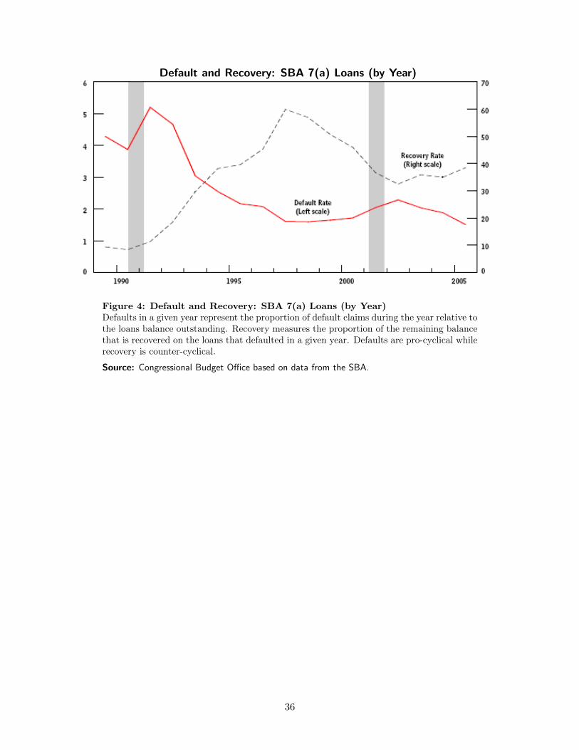
Default and Recovery: SBA 7(a) Loans (by Year)

Figure 4: Default and Recovery: SBA 7(a) Loans (by Year)Defaults in a given year represent the proportion of default claims during the year relative tothe loans balance outstanding. Recovery measures the proportion of the remaining balancethat is recovered on the loans that defaulted in a given year. Defaults are pro-cyclical whilerecovery is counter-cyclical.

Source: Congressional Budget Office based on data from the SBA.

36

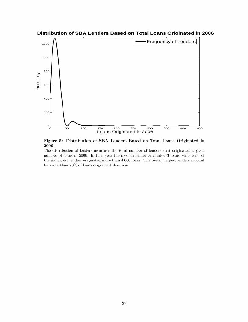
0 50 100 150 200 250 300 350 400 4500

200

400

600

800

1000

1200

Loans Originated in 2006

Freq

uenc

yDistribution of SBA Lenders Based on Total Loans Originated in 2006

Frequency of Lenders

Figure 5: Distribution of SBA Lenders Based on Total Loans Originated in2006The distribution of lenders measures the total number of lenders that originated a givennumber of loans in 2006. In that year the median lender originated 3 loans while each ofthe six largest lenders originated more than 4,000 loans. The twenty largest lenders accountfor more than 70% of loans originated that year.

37

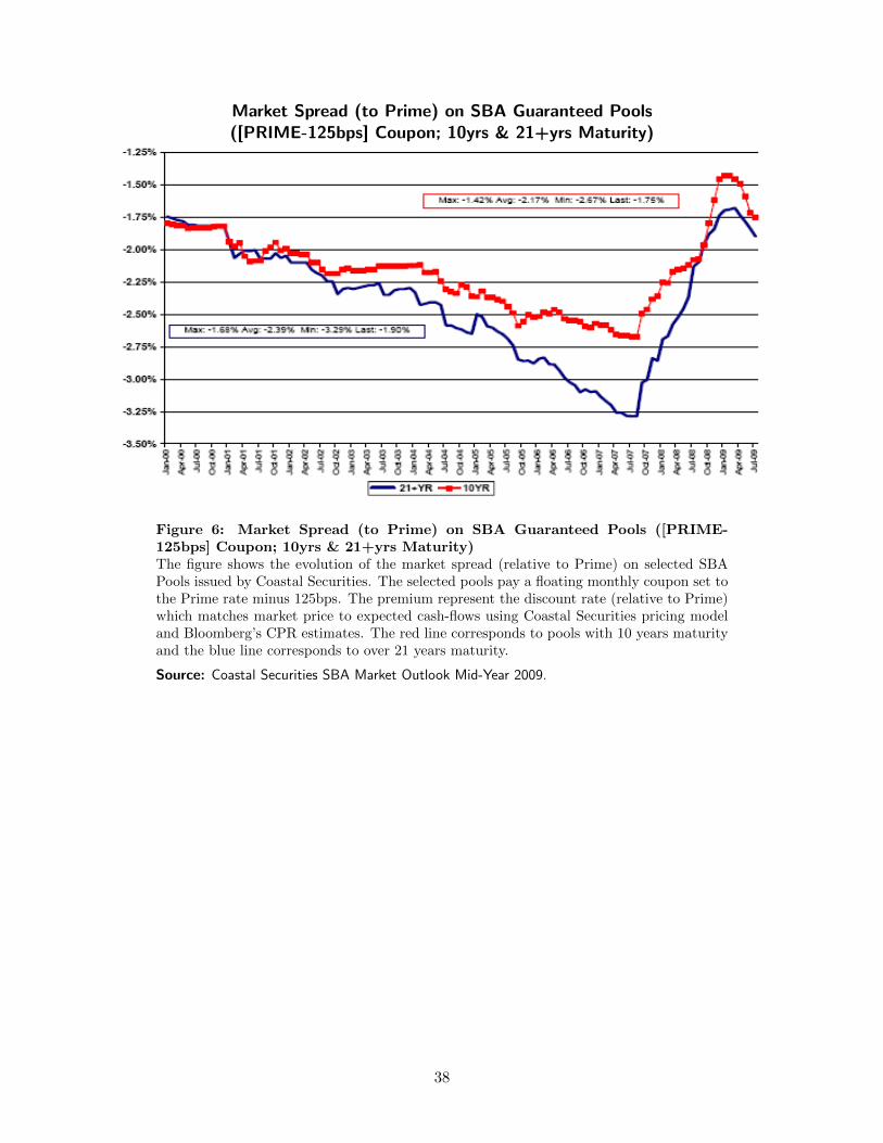
Market Spread (to Prime) on SBA Guaranteed Pools([PRIME-125bps] Coupon; 10yrs & 21+yrs Maturity)

Figure 6: Market Spread (to Prime) on SBA Guaranteed Pools ([PRIME-125bps] Coupon; 10yrs & 21+yrs Maturity)The figure shows the evolution of the market spread (relative to Prime) on selected SBAPools issued by Coastal Securities. The selected pools pay a floating monthly coupon set tothe Prime rate minus 125bps. The premium represent the discount rate (relative to Prime)which matches market price to expected cash-flows using Coastal Securities pricing modeland Bloomberg’s CPR estimates. The red line corresponds to pools with 10 years maturityand the blue line corresponds to over 21 years maturity.

Source: Coastal Securities SBA Market Outlook Mid-Year 2009.

38

Jan2006 Apr2006 Jul2006 Oct2006 Jan2007 Apr2007 Jul2007 Oct2007 Jan2008 Apr2008 Jul2008−200

−100

0

100

200

300

400

Date

Prem

ium A

bove

Tre

asur

y (bp

s) Premium (bps Above Treasury) of SBA Guaranteed Pools

Premium (bps)Average Monthly Premium (bps)

Figure 7: Premium (bps above Treasury) of SBA Guaranteed PoolsThe figure shows the market premium (relative to Treasury) on selected SBA Pools issuedby Coastal Securities between January 2006 and May 2008. The selected pools pay afloating monthly coupon set to the Prime rate plus a fixed spread. The premium representthe discount rate (above the Treasury) which matches market price to expected cash-flowsusing a Monte Carlo pricing model which incorporates the historic default and prepaymentprobabilities derived from the SBA database. The dots represent the premium on individualpools and the circles represent the mean monthly premia on the selected pools.

39

0 2 4 6 8 10 12 14 160

0.5

1

1.5

2

2.5

3

3.5

4

Loan Age (years)

Defa

ult R

ate

(%)

Historic Default Frequency (by Loan Age) of SBA Loans

Default Frequency

Figure 8: Historic Default Frequency (by Loan Age) of SBA LoansDefault frequencies measure the proportion of loans that default from cohort formation toa given loan year. The default frequencies are estimated using historic SBA data from1988-2008. During this period defaults peaked in the loan’s third year.

40

0 2 4 6 8 10 12 14 160

1

2

3

4

5

6

7

8

9

10

Loan Age (years)

Prep

aym

ent R

ate

(%)

Historic Prepayment Frequency (by Loan Age) of SBA Loans

Prepayment Frequency

Figure 9: Historic Prepayment Frequency (by Loan Age) of SBA LoansPrepayment frequencies measure the proportion of loans that prepay from cohort formationto a given loan year. The prepayment frequency are estimated using historic SBA data from1988-2008. During this period prepayment peaked in the loan’s fourth year.

41

1990 1992 1994 1996 1998 2000 2002 2004 20060

0.5

1

1.5

2

2.5

3

3.5

4

4.5

5

Year

Defau

lt Rate

(%)

Default Rates of SBA Loans − by Lender Size

Large Lender DefaultMedium Lender DefaultSmall Lender Default

Figure 10: Default Rates of SBA Loans - by Lender SizeDefaults in a given year represent the proportion of default claims during the year relativeto the loans outstanding for each lender. Then in each year the default rates are averagedout based on the lender size according to three categories. The categories are large lenders,medium lenders, and small lenders. The small lenders are the ones that originated lessthan the median that year. Large lenders are alternatively defined as the top 1st percentile.medium lenders are the rest.

42

1990 1992 1994 1996 1998 2000 2002 2004 20060

2

4

6

8

10

12

14

Year

Prep

ayme

nt Ra

te (%

) Prepayment Rates of SBA Loans − by Lender Size

Large Lender PrepaymentMedium Lender PrepaymentSmall Lender Prepayment

Figure 11: Prepayment Rates of SBA Loans - by Lender SizePrepayments in a given year represent the proportion of prepayment claims during theyear relative to the loans outstanding for each lender. Then in each year the prepaymentrates are averaged based on the lender size according to three categories. The categoriesare large lenders, medium lenders, and small lenders. The small lenders are the ones thatoriginated less than the median that year. Large lenders are alternatively defined as the top1st percentile. medium lenders are the rest.

43