1We thank the James M. Kilts Center, GSB, University of Chicago for the data used in this study, and JudyChevalier, Anil Kashyap Peter Rossi, the editor and an anonymous referee for comments on earlier drafts. The firstauthor thanks the NSF and the Sloan Foundation for support.

Why Does the Average Price Paid Fall

During High Demand Periods?1

Aviv Nevo Northwestern University and NBER

Konstantinos Hatzitaskos University of California, Berkeley

July 2006

ABSTRACTFor many products the average price paid by consumers falls during periods of highdemand. We use information from a large supermarket chain to decompose thedecrease in the average price into a substitution effect, due to an increase in the shareof cheaper products, and a price reduction effect. We find that for almost all theproducts we study the substitution effect explains a large part of the decrease. Weestimate demand for these products and show the price declines are consistent witha change in demand elasticity and the relative demand for different brands. Ourfindings suggest, that for the data we examine, loss-leader models of retailcompetition are not the main explanation for price declines.

2CKR discuss the composition bias and report that “the majority of the category-level price declines documentedin Table 3 remain statistically significant using fixed-weight price indices.” We find results that are essentially identicalto their variable weight price index results, but find smaller effects when we use a fixed weights index. This suggeststhat composition bias might be important.

3Our demand results are very similar to CKR’s findings, which they use to examine the alternative theoryproposed by Warner and Barsky (1995). As we discuss below, we differ in how we interpret the results.

1

1. Introduction

A number of previous papers document that retail prices for many products tend to fall

during periods of peak demand. Warner and Barsky (1995) examine four months of daily prices of

several items and find that prices tend to be marked down during weekends and before Christmas,

periods of (exogenously) high demand. MacDonald (2000) documents a decrease in the price of food

products at seasonal demand peaks. Chevalier, Kashyap and Rossi (2003) (CKR, hereafter) use

weekly item-level scanner data from a single retailer in Chicago, and find that prices fall during

periods of high demand. As we discuss in detail below, they examine different theories that

potentially explain the price declines and conclude that the decline in prices is best explained by loss

leader models of advertising (Lal and Matutes, 1994).

In this paper, we offer an alternative explanation to the decline in the average price. Our

explanation is based on a change in brand-level demand. We focus on two changes: a change in

price sensitivity, that would lead to lower equilibrium prices, and a change in brand preferences

within a product category, that leads to a substitution towards cheaper products. Using CKR’s data

we find the following support for our explanation. First, we find a difference in the decline between

a fixed and variable weights price index, which is consistent with a change in the composition of

brands.2 Next, we find that for tuna, which faces a high demand peak during Lent, much of the

increase in the quantity sold is due to two products. These products, which are relatively cheap,

nearly triple their market share and interestingly do not reduce their prices. Some of the competitors

indeed lower their prices, in what seems to be a response to the decline in their market shares.

Looking at other categories, which CKR define as having peak demand periods, we estimate brand-

level demand and find, as predicted by our explanation, that demand is more price sensitive and that

the brand preferences change during periods of high demand.3

2

There are three general lessons that can be learned from our analysis. First is the importance

of considering product differentiation and its implications for the results. CKR advocate the

importance of incorporating retail behavior, but do so at the cost of treating the product as

(essentially) homogenous. We, on the other hand, place more emphasis on product differentiation,

and therefore interpret the results differently. Second, our results show that one has to be careful in

using prices paid by consumers to make inferences about supply side behavior. The observed prices

might be driven, at least in part, by consumer behavior and not by pricing. Third, sales are a major

source of nominal price variation in many retail markets. Therefore, understanding what drives sales,

and price rigidity during non-sale periods, has implications for the macro-economy (Warner and

Barsky, 1995, CKR, Bils and Klenow, 2004.) Our results are suggestive of economy-wide patterns,

but since they are based on data from one retailer for a few product categories, require verification

through further research using additional data.

2. Previous Findings and Explanations

Several papers have documented the decline of prices during periods of high demand and

have offered various theoretical explanations. The first class of theories are those that suggest that

demand might be more elastic than usual during peak demand periods (for example, Bils,1989, and

Warner and Barsky, 1995). The Warner and Barsky model suggests that, with fixed costs of search

and travel between stores, consumers will search more during high demand periods. Thus, the

demand facing a retailer will be more price elastic and the optimal price is lower.

A second class of models are those that focus on dynamic interactions between retailers. In

the spirit of Rotemberg and Saloner (1986), tacit collusion is sustained when the gains from

defection (i.e., charging a price below the collusive level) in the current period are lower than the

expected losses in future periods due to punishment. The incentive to cheat is highest during periods

of peak demand since the current gains from cheating are higher. Therefore, the price level that can

be sustained during high demand periods is lower.

The third class of models are loss leader advertising models (Lal and Matutes, 1994). In

4We thank a referee for pointing this out.

3

these models, consumers do not know the prices of the goods until they arrive at the store. They pay

a transportation cost to get to the store and to go from one store to another. If this cost is high

enough, the retailers will charge consumers their reservation price (which is assumed identical for

all consumers) once they arrive at the store, and their transportation cost is sunk. Consumers foresee

this strategy and therefore do not shop. The retailer’s solution is to commit to a particular price by

advertising it. If advertising was costless then retailers would advertise all products. Lal and Matutes

assume that retailers pay an advertising cost per item advertised. For items not advertised consumers

assume that they will be charged their reservation. In this model prices are not pinned down: any

of the goods could be discounted enough to attract consumers. However, as CKR point out, if prices

have to be non-negative, then it is possible that the retailer cannot give a large enough discount on

some items, and can only give this discount through high demand products.

Even before going to the data there are a couple of reasons to be somewhat suspicious of

the loss leader theory. First, which product goes on sale is determined by the non-negativity

constraint: a retailer puts the product on sale that allows a large enough discount. While this effect

is clear in a simple model, it seems somewhat unlikely that this constraint is binding in the

marketplace. Indeed, if it did, we should expect to see prices at or near zero.4 Second, and somewhat

related, while in the model high demand is relative to other products, when taking the model to the

data, CKR interpret high demand relative to the typical demand for the product. Many of the

products CKR examine are a small part of the overall expenditure of a household in any given

shopping trip. For example, a can of tuna costs roughly 80 cents. Even if a household buys five cans

during a high demand period and the discount is 20 cents, or 25 percent (a much larger discount than

what we see in the data), then the savings are one dollar. Surely there are other ways to offer such,

or much larger, savings.

CKR find the following in their data. First, retail prices go down during periods of high

demand. They report summary statistics from regressions using item-level product aggregates and

report detailed results from a variable weight category-level price index. CKR show that prices

4

decline even during periods of product specific peak demand (e.g., tuna during Lent). The first two

sets of models, discussed above, offer an explanation for why prices are low during the overall high

demand periods, but not during idiosyncratic peak demand periods. Second, they find smaller, or

no effects, using average acquisition costs and a proxy for retail margins (retail price minus the

average acquisition cost divided by price). Third, by estimating category-level demand regressions

they show that demand is not more elastic during periods of overall high demand (Christmas and

Thanksgiving), providing direct evidence against the Warner and Barsky theory. Finally, they show

that a larger fraction of category sales are accounted for by advertising specials during periods of

peak demand.

3. Our Explanation

In this section we offer an alternative explanation as to why the average price declines during

peak demand periods. We believe our explanation is an important aspect of the data generating

process, but we do not suggest it characterizes it completely, and may operate alongside the theories

discussed in the previous section. Our explanation is consistent with prior findings, surveyed in the

previous section. We discuss the empirical implications that allow us to separate our explanation

from alternative theories and we test these implications in the next sections.

Our explanation relies on a change in brand-level demand. We focus on two changes in

particular: a change in demand elasticity and changes in relative demand for different brands during

peak demand for the category. The shift in the aggregate, or average, price sensitivity can occur for

several reasons. The demand of certain households might increase more than others. Consider, for

example, demand for tuna during Lent. If price sensitivity varies by household, then the aggregate

price sensitivity will differ between Lent and non-Lent periods. Alternatively, for a given household

price sensitivity might vary if the use of the product changes.

While overall demand for a product (e.g., tuna) might increase, we claim that the increase

might be different for different brands (e.g., StarKist). Basically preferences may not be homothetic

with respect to combinations of quality and quantity. For example, there might be a shift in relative

5

household-level demand for different brands. Consider the case of canned tuna. It could be used for

various dishes, including tuna salad or tuna casserole. These different uses might require different

quality. For example, tuna casserole might require a lower quality brand. If during Lent tuna

casserole is eaten more frequently than tuna salad, relative to non-Lent periods, then the relative

demand for brands will change disproportionately. Additionally, just as is the case for price

elasticity, even if brand preferences at the household level remain constant, there could be a change

in aggregate demand because different households increase their demand.

There are several implications of our explanation that distinguish it from alternatives. First,

our explanation implies that the effect on a category-level price index will be different if one uses

a fixed-weights index versus a variable weight index. Since we claim there is a change in brand

preferences during some periods of high demand, then the change in weights is systematic, and we

expect the fixed weights index to give a different answer. In particular, if the shift is towards cheaper

brands, then we expect the fixed weights index to exhibit smaller drops during high demand periods.

Indeed, if all that is happening is a shift between brands, then this index should not drop at all.

Second, in order to test our explanation directly we look at brand-level data. We examine

prices of different brands to see which brands reduce their prices during periods of high demand.

We also examine quantities to see if all brands experience an increase in demand during periods of

category high demand.

Third, we estimate a brand-level demand system, allowing price sensitivity and brand

preferences to change between high demand periods and other periods. We test if brand preferences

vary during high period demand. Furthermore, we test if price sensitivity varies during periods of

product specific high demand (and not during overall demand periods, as CKR test).

4. Data and Category-Level Analysis

4.1 Data

The data set used for the analysis is the same as the one used by CKR, and comes from the

Dominick’s Finer Foods (DFF) database at the University of Chicago Graduate School of Business.

6

The data are described further in Appendix A and by CKR, and can be found at

http://www.gsb.uchicago.edu/kilts/research/db/dominicks/. Definitions of key variables follow CKR,

as detailed in Appendix A.

We focus on the categories that CKR identified as having high demand periods, and we follow

their definitions of a-priori high demand periods. The categories we study are tuna, beer, oatmeal,

cheese and snack crackers. CKR study two additional seasonal categories: eating soup and cooking

soup. We decided to not examine these categories, since we felt uncomfortable in our ability to

classify products into each category. We also do not study the non-seasonal categories identified by

CKR (analgesics, cookies, crackers and dish detergent), since they seem to have little relevance for

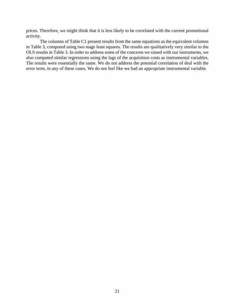
our explanation. Summary statistics for the main variables for each of the product categories we used

are displayed in Table A1.

For each category we include the top 30 products. For the most part a product is a UPC.

However, over the period there are several cases where the product was unchanged but the UPC was

changed for technical reasons. In these cases we combined these UPCs into a single product. The

30 products jointly account for a significant share of each category, as can be seen in the last row of

Table A1.

4.2 Category-Level Analysis

We start by examining category level price indices. The indices are computed in the following

way. The price data are collected by store, product and week. Let be the logarithm of price per

ounce of product j at store s in week t. The price index in time t is

where are weights. We report results using two price indices. The first is a variable weight price

index, in which is the revenue share of product j sold in store s in week t of the total revenue sold

in t. The second is a fixed weight in which is the revenue share of product j sold in store s in the

5For the purpose of this count, and the discussion below, we exclude the Superbowl period that was notexamined by CKR.

7

sample period of the total revenue sold in the sample period, normalized so the shares in each week

sum to one. The variable weight index is analogous to the one used by CKR.

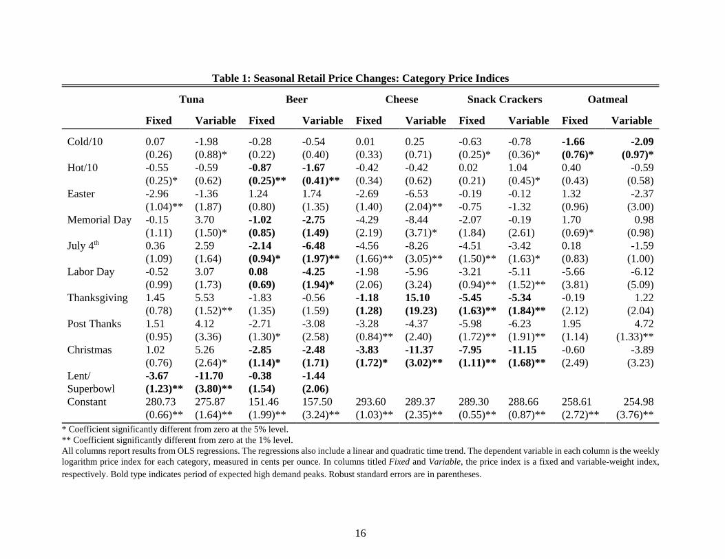
Table 1 reports results from OLS regressions where the dependent variable is the weekly price

index in each category. In columns titled Fixed and Variable, the price index is a fixed- and variable-

weight price index, respectively. Bold type indicates a period of expected high demand peaks,

following CKR’s classification.

Examining the results in the Variable columns, we generally find results similar to CKR. The

price index tends to go down during expected high demand periods. Out of the 11 periods of expected

high demand, 8 have a statistically significant decline in the variable weights price index.5 For the

Cheese and Snack Crackers categories, we tend to find price declines during periods when high

demand is not expected (Easter, July 4th and Memorial Day for Cheese, and July 4th, Labor Day and

Post Thanksgiving for Snack Crackers) that are of the same order of magnitude as the declines during

high demand periods.

The results in the Fixed columns tend to present a somewhat different picture. The number

of statistically significant coefficients is similar to the results using the variable weight price index.

However, the economic magnitude of the coefficients drops. The results suggest that the average

decline during the 11 peak demand periods is approximately 2.5%. Excluding the two coefficients

that have different signs, the median (average) ratio of the fixed weights result to the variable weight

result is 0.52 (0.60). In some cases the ratio is even lower. For example, the coefficient on Lent in

the tuna category using the fixed-weights index, is roughly a third of the same coefficient using a

variable-weights index.

The prices of tuna during Christmas and Thanksgiving provide us with another opportunity

to see how the two price indices differ. The results in the variable column suggest that the price of

tuna during Christmas and Thanksgiving is higher. One could think of this as evidence for the loss-

leader story: since the demand for tuna is low during these periods, they are not used as loss-leaders

8

and are therefore less likely to be on sale. However, when we look at the results in the Fixed column

a different picture emerges. It is not that tuna is more expensive, but that there seems to be

substitution towards more expensive brands.

It is well-known that the difference between fixed and variable weights price indices allows

us to check for the existence of a composition bias (Jorgenson and Griliches, 1967; Bee Yan and

Roberts, 1986). Our results suggest that a change in composition is an important part of the observed

decline in average prices. However, if this was all that was happening then the fixed-weights index

would not change. The fact that it is decreasing suggests that at least some products are reducing their

price.

The question then is whether the drop in retail prices is driven by retail or manufacturer

behavior. CKR examine this by repeating the analysis using an index based on an average acquisition

cost of the inventory and the margin relative to this cost. They conclude that retailer behavior is the

driving force. We repeated their analysis and find results similar to theirs. However, this analysis,

based on log prices, does not allow us to address the economic, as opposed to the statistical,

significance of the change in average acquisition cost versus retail markup.

The results in Appendix B repeat the analysis of Table 1 using as the dependent variable the

levels of the variables (retail price, and average acquisition cost). Based on these results breaking

down the variation is straightforward. The breakdown varies a bit between the categories and whether

one uses the variable or fixed weights results. However, it seems like in a typical case the decrease

in the average acquisition cost accounts for 40-50% of the decline in the retail price. The fraction is

generally larger in the tuna and oatmeal categories during their peak demand periods, suggesting that

retailer behavior is relatively more important in categories that have expected peaks during periods

of overall high demand, while retail behavior is less significant in those cases where the demand peak

is category specific. We recall that the way CKR propose to separate their model and some of the

alternatives is by offering an explanation for price reduction during periods of category specific peak

demand.

There are a couple of reasons to believe that even these results underestimate the importance

9

of wholesale price reductions. First, as pointed out by CKR (on page 19) these average acquisition

costs are not the economic replacement cost, which is what we want, rather they are historical

acquisition costs. Therefore, the average acquisition price is an average of recent wholesale prices,

and thus probably underestimates the decline in the economic wholesale price. Second, in reality the

wholesaler-retailer contracts are quite complex and include various incentives that will not appear

in the average acquisition cost. This will also lead one to underestimate the importance of wholesale

prices.

5. Product-level Analysis

In the previous section we showed that a change in the composition of brands explains a significant

fraction of the decline in the category-level variable weight price index. We also showed that the data

suggest a decline in wholesale prices is a significant part of the decline in retail prices, especially for

products with category specific peak demand periods. CKR (Table 2) also summarize results using

product aggregates that will not suffer from this composition bias. In this section, we provide analysis

using product-level data to support the findings of the previous section.

5.1 Product-level price and quantity regressions

Before analyzing the data from all categories, we take a closer look at the canned tuna

category. We focus on tuna for several reasons. First, this category seems to have the most robust

results in support of the CKR loss leader model (both during peak and non peak demand). Second,

as CKR note, and as we discussed in Section 2, a key to separating the loss leader model from

alternatives is to focus on products that have their own seasonal peak demand. The tuna category is

probably the cleanest example of such an effect among the categories we study. Beer also has well

defined idiosyncratic peak demand periods that are not overall peak demand periods. However, the

results in Table 1 do not seem to support the loss leader story. Furthermore, the beer category in this

data set is not representative of the US as a whole. In the national market Budweiser is a clear market

leader, while in our data Miller has a larger market share. To the extent that the pricing decisions are

10

impacted by other retailers and other markets, then this data set is not a good place to study the beer

category.

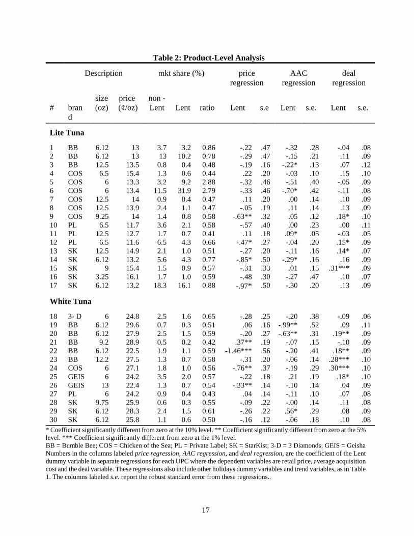
In Table 2 we present brand level statistics for the top 30 products in the tuna category. Each

row presents results for a different product. In the fourth column we present the average price per

ounce for each product. The distribution of prices is roughly bi-modal. For Lite Tuna, the prices range

from 12 cents per ounce to 16 cents per ounce. White Tuna is more expensive, with prices ranging

between 23 to 30 cents per ounce.

Columns (v)-(vii) present the product-level market shares during non-Lent periods, during

Lent, and the ratio of the two, respectively. The pattern is clear: the quantity sold of light tuna

increases during Lent, while there is no increase, even a slight decrease, in the quantity sold of the

higher quality white tuna. This suggests that even within the tuna category there is a differential

demand peak. Furthermore, it suggests that indeed a variable weight price index will tend to find a

decrease in the price during Lent, even without any changes in prices.

Probably the most striking statistic in Table 2 is the change in the market share of two

products: Chicken of the Sea 6 ounce light tuna and 6 ounce light tuna in oil (rows 5 and 6). These

two products almost triple their market shares during Lent. At the same time all other light tuna,

including Star Kist 6.12 ounce cans of light tuna (rows 17 and 14) and Private Label 6.5 ounce cans

(rows 10 and 12), the number 1 and 3-5 top-selling products during non-Lent periods, are losing

market shares. This difference could be driven by an exogenous increase in the demand for Chicken

of the Sea (i.e., a change in brand preference) or by an endogenous increase in demand due to pricing

or promotional activities.

The last columns in the table present results from separate product-level regressions. An

observation in this regression is at the product-week level, aggregating across stores by revenue. In

each regression, retail price (or average acquisition cost or deal) is regressed on a Lent dummy

variable and other holiday dummy variables. These regressions are identical to those used to produce

the results in Table 1, but the dependent variable is the price of the product rather than a category

price index. The table reports only the Lent coefficient and the robust standard error. A negative

6The price regressions are in levels and the dependent variable is measured in cents per ounce. For brands 5and 6 they suggest roughly a 2 cents decrease, for a 6 ounce can, which is normally priced around 80 cents.

11

coefficient denotes a product that is systematically priced lower during Lent.

There are several patterns in these coefficients. First, in the light tuna category the products

that have significant price decreases during Lent are products that are losing market shares (even

despite the price reductions). The main two products gaining market shares do not have significant

price decreases. Not only are the effects not statistically significant but the economic significance is

small.6 These results suggest that the increase in market share we saw in columns (v)-(vii) is not

driven by pricing. Second, three out of the seven products with significant price reductions during

Lent are white tuna, which we saw does not exhibit a seasonal shock. Third, some of the average

acquisition costs seem to go down during Lent. However, there seems to be low correlation between

the prices that exhibit reductions in average acquisition cost and those that decrease the retail price.

There are two ways to interpret these results: CKR claim that this is evidence in support of the claim

that retailers behavior is driving pricing. Alternatively, these results could be driven by the poor

quality of average acquisition cost as a proxy for the wholesale prices, as we previously discussed.

Fourth, many of the products that have increased advertising, as measured by the deal code, are those

that are losing market share.

Together, these patterns are not consistent with the loss-leader story. The products that are

reducing their prices and increasing their advertising during Lent are not those that are facing an

increase in demand, but rather those that are losing market share.

5.2 Product-level demand

In order to generalize the product-level analysis to other categories, in this section we present

results from a product- level demand model and focus on two sets of results across the different

product categories. First, we look for evidence that brand preferences are changing during peak

demand periods. Second, we ask if price sensitivity changes during product-specific peak demand

periods.

12

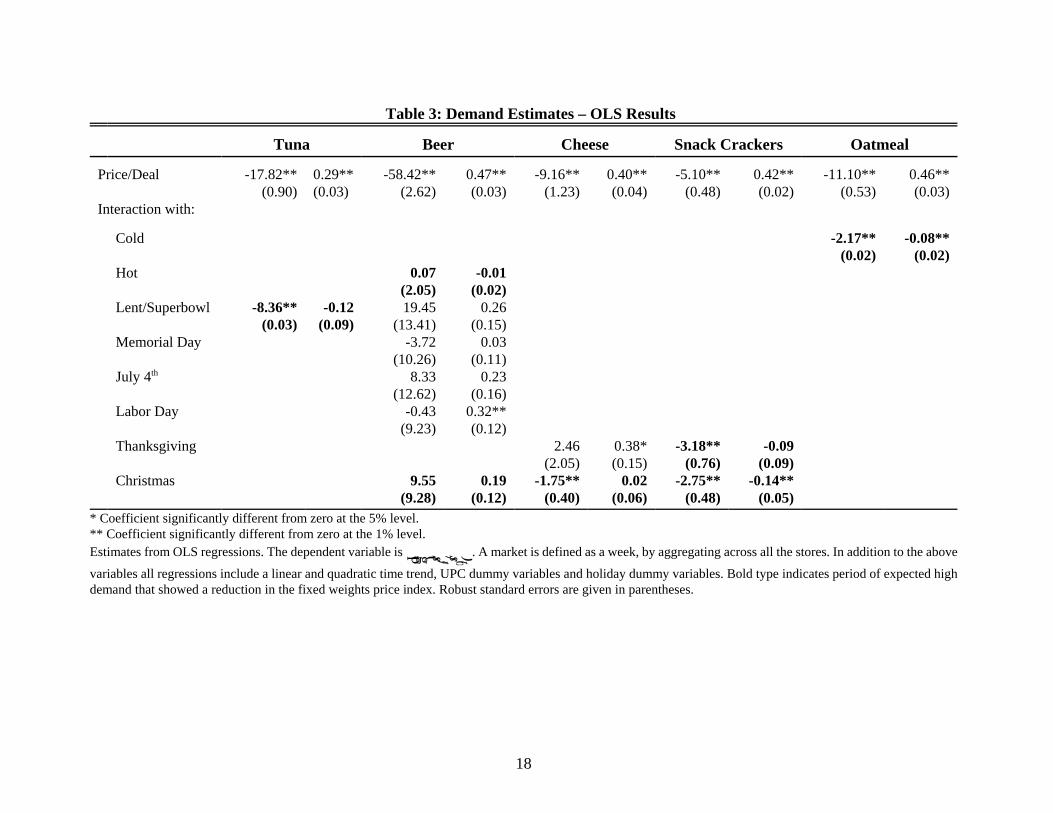
The results presented in Table 3 are computed from an aggregate Logit model and are

estimated using OLS. The model, and the identifying assumption, are presented in Appendix C. CKR

also examine a demand model. Interestingly, despite using a very different demand model

qualitatively their results are similar to ours. Indeed, below we point out that we could make one of

our main points using their results.

In order to test the hypothesis that brand preferences are changing during peak demand

periods, we interact the brand-specific effects with peak demand variables and test the joint

hypothesis that the interaction terms are zero. The hypothesis that the interactions are zero is rejected

quite strongly in all categories, not just tuna. The relative demand for different brands is changing,

even once we control for pricing and advertising activities.

Next, we explore a change in price sensitivity during periods of peak demand by including

interactions of price and peak demand variables. The results are presented in the first column for each

category of Table 3. Eight out of the twelve expected high demand periods in the table have negative

interaction terms. A negative interaction implies that demand is becoming more price sensitive and

provides a rationale for price drops. However, many of these interactions are not statically significant.

Recall that many of the expected high demand periods did not exhibit significant drops in the fixed

weights price index. Therefore, the drop in the average price for these periods is explained by

substitution towards cheaper brands, a composition effect, and we do not need a change in price

sensitivity to explain the reduction in the average price paid by consumers. For this reason we

highlight in bold type the seven periods that exhibit a significant decline in the fixed price index

during expected periods of high demand. Five out of seven of these interactions are negative and

statistically significant.

The second column for each category of Table 3 examines the interaction of the deal variable

and the expected periods of high demand. In most cases the interaction between advertising and peak

demand is either negative or not statistically significant.

As we discuss briefly in Appendix C, there are several potential problems with our demand

system. One interesting robustness check is to compare our results to CKR’s Table 6. Despite several

7Beer during Christmas and hot, eating soups and oatmeal during cold, cooking soups, cheese and snackcrackers during Thanksgiving and Christmas, and tuna during Lent.

8Seven are negative and statistically significant and one corresponds to a period where the fixed weight pricedoes not drop.

13

differences between our specifications, the results are remarkably similar. Using their results one

could examine the change in price elasticity during peak demand for 11 periods.7 of which eight

periods overlap with our twelve interactions. Their results are essentially identical to ours: eight out

of the eleven interaction terms match the change in the fixed weights price index.8

6. Conclusions

In this paper we re-examine an empirical puzzle: why do prices go down during peak demand

periods? We offer an explanation that is based on a change in the relative demand for different brands

and a change in price sensitivity. Our empirical analysis offers results in support of our explanation

and evidence that is less consistent with the alternative loss leader model as the primary explanation

of the observed price patterns.

In support of our explanation, we find that the reduction in a fixed weights price index is

much smaller than the reduction in the variable weight price index, which is consistent with a change

in the composition of brands and a substitution towards cheaper brands. We also find that in the tuna

category the brands that face the highest increase in demand are not the ones reducing their prices.

Instead, it is those brands that are losing market share that reduce their prices. Finally, estimates of

brand-level demand suggest that changes in brand preferences are statistically significant and that the

price sensitivity is higher (in absolute value) during periods of peak demand.

There are several ways in which our findings suggest that the loss leader model does not fully

explain the observed patterns. First, we find that the effects on fixed weight price indices are less

significant, both economically and statistically, than the effects on variable weight price indices. For

those categories (like tuna and oatmeal) that CKR claim are the key to separating their model from

alternatives, we find that average acquisition cost plays an important role in the price reductions.

Second, examining the tuna category more carefully we find that not all brands face the same increase

14

in demand, and that those brands that face the higher increase are not the ones reducing their prices

(or increasing advertising). We find the disproportionate nature of the change in product-level

demand in the other categories we examine as well.

The explanation we provide seems to be consistent with the data we examine and the results

are suggestive of economy-wide patterns. However, before one can generalize more broadly from this

data set verification, through further research using additional data is required. Finally, we do not

claim that our explanation is the only reason for price reductions, or even that it is the only reason

for price reduction during peak seasonal demand. More likely it is working jointly with some of the

other effects like those offered by the Rotemberg Saloner (1986) theory, the Warner Barsky (1995)

model, or the loss leader story.

References

Bee Yan AW and Mark Roberts. “Measuring Quality Change in Quota-Constrained Import Markets.”

Journal of International Economics, 1986, 21, 45-60.

Bils, Mark. “Pricing in a Customer Market.” Quarterly Journal of Economics, November 1989,

104(4), pp. 699-717.

Bils, Mark and Peter Klenow. “Some Evidence on the Importance of Sticky Prices,” Journal of

Political Economy, 2004, 112(5), 947-985.

Chevalier, Judith A., Kashyap, Anil K. and Rossi, Peter E. “Why Don’t Prices Rise During Periods

of Peak Demand? Evidence from Scanner Data.” American Economic Review, June 2003,

93(1), pp. 15-37.

Jorgenson, Dale W. and Zvi Griliches,.“The explanation of productivity change.” Review of

Economic Studies, 1967, 34, 249-283.

Lal, Rajiv and Matutes, Carmen. “Retail Pricing and Advertising Strategies.” Journal of Business,

July 1994, 67(3), pp. 345-70.

MacDonald, James M. “Demand, Information and Competition: Why Do Food Prices Fall at

Seasonal Demand Peaks?” Journal of Industrial Economics, March 2000, 48(1), pp.27-45.

15

Pashigian, Peter B. “Demand Uncertainty and Sales: A Study of Fashion and Markdown

Pricing.”American Economic Review, December 1988, 78(5), pp. 936-53.

Pashigian, Peter B. and Bowen Brian. “Why Are Products Sold on Sale? Explanations of Pricing

Regularities.” Quarterly Journal of Economics, November 1991, 106(4), pp. 1015-38.

Rotemberg, Julio J. And Saloner, Garth. “A Supergame-Theoretic Model of Price Wars During

Booms.” American Economic Review, June 1986, 76(3), pp. 54-63.

Warner, Elizabeth J. And Barsky, Robert B. “The Timing and Magnitude of Retail Store Markdowns:

Evidence from Weekends and Holidays.” Quarterly Journal of Economics, May 1995,

110(2), pp. 321-52.

16

Table 1: Seasonal Retail Price Changes: Category Price Indices

Tuna Beer Cheese Snack Crackers Oatmeal

Fixed Variable Fixed Variable Fixed Variable Fixed Variable Fixed Variable

Cold/10

Hot/10

Easter

Memorial Day

July 4th

Labor Day

Thanksgiving

Post Thanks

Christmas

Lent/SuperbowlConstant

0.07(0.26)-0.55(0.25)*-2.96(1.04)**-0.15(1.11)0.36(1.09)-0.52(0.99)1.45(0.78)1.51(0.95)1.02(0.76)-3.67(1.23)**280.73(0.66)**

-1.98(0.88)*-0.59(0.62)-1.36(1.87)3.70(1.50)*2.59(1.64)3.07(1.73)5.53(1.52)**4.12(3.36)5.26(2.64)*-11.70(3.80)**275.87(1.64)**

-0.28(0.22)-0.87(0.25)**1.24(0.80)-1.02(0.85)-2.14(0.94)*0.08(0.69)-1.83(1.35)-2.71(1.30)*-2.85(1.14)*-0.38(1.54)151.46(1.99)**

-0.54(0.40)-1.67(0.41)**1.74(1.35)-2.75(1.49)-6.48(1.97)**-4.25(1.94)*-0.56(1.59)-3.08(2.58)-2.48(1.71)-1.44(2.06)157.50(3.24)**

0.01(0.33)-0.42(0.34)-2.69(1.40)-4.29(2.19)-4.56(1.66)**-1.98(2.06)-1.18(1.28)-3.28(0.84)**-3.83(1.72)*

293.60(1.03)**

0.25(0.71)-0.42(0.62)-6.53(2.04)**-8.44(3.71)*-8.26(3.05)**-5.96(3.24)15.10(19.23)-4.37(2.40)-11.37(3.02)**

289.37(2.35)**

-0.63(0.25)*0.02(0.21)-0.19-0.75-2.07(1.84)-4.51(1.50)**-3.21(0.94)**-5.45(1.63)**-5.98(1.72)**-7.95(1.11)**

289.30(0.55)**

-0.78(0.36)*1.04(0.45)*-0.12-1.32-0.19(2.61)-3.42(1.63)*-5.11(1.52)**-5.34(1.84)**-6.23(1.91)**-11.15(1.68)**

288.66(0.87)**

-1.66(0.76)*0.40(0.43)1.32(0.96)1.70(0.69)*0.18(0.83)-5.66(3.81)-0.19(2.12)1.95(1.14)-0.60(2.49)

258.61(2.72)**

-2.09(0.97)*

-0.59(0.58)-2.37

(3.00)0.98

(0.98)-1.59

(1.00)-6.12

(5.09)1.22

(2.04)4.72

(1.33)**-3.89

(3.23)

254.98(3.76)**

* Coefficient significantly different from zero at the 5% level.** Coefficient significantly different from zero at the 1% level.All columns report results from OLS regressions. The regressions also include a linear and quadratic time trend. The dependent variable in each column is the weeklylogarithm price index for each category, measured in cents per ounce. In columns titled Fixed and Variable, the price index is a fixed and variable-weight index,respectively. Bold type indicates period of expected high demand peaks. Robust standard errors are in parentheses.

17

Table 2: Product-Level Analysis

Description mkt share (%) priceregression

AACregression

dealregression

# brand

size(oz)

price (¢/oz)

non -Lent Lent ratio Lent s.e Lent s.e. Lent s.e.

Lite Tuna

1234567891011121314151617

BBBBBB COSCOSCOSCOSCOSCOSPL PL PL SK SK SK SK SK

6.126.1212.5

6.566

12.512.59.25

6.512.5

6.512.56.12

93.256.12

1313

13.515.413.313.4

1413.9

1411.712.711.614.913.215.416.113.2

3.713

0.81.33.2

11.50.92.41.43.61.76.52.15.61.51.7

18.3

3.210.2

0.40.69.2

31.90.41.10.82.10.74.31.04.30.91.0

16.1

0.860.780.480.442.882.790.470.470.580.580.410.660.510.770.570.590.88

-.22-.29-.19.22

-.32-.33.11

-.05-.63**

-.57.11

-.47*-.27

-.85*-.31-.48

-.97*

.47

.47

.16

.20

.46

.46

.20

.19

.32

.40

.18

.27

.20

.50

.33

.30

.50

-.32-.15

-.22*-.03-.51

-.70*.00.11.05.00

.09*-.04-.11

-.29*.01

-.27-.30

.28

.21

.13

.10

.40

.42

.14

.14

.12

.23

.05

.20

.16

.16

.15

.47

.20

-.04.11.07.15

-.05-.11.10.13

.18*.00

-.03.15*.14*

.16.31***

.10

.13

.08

.09

.12

.10

.09

.08

.09

.09

.10

.11

.05

.09

.07

.09

.09

.07

.09

White Tuna

18192021222324252627282930

3- DBBBBBB BB BB COSGEISGEISPL SK SK SK

66.126.12

9.26.1212.2

66

136

9.756.126.12

24.829.627.928.922.527.527.124.222.424.225.928.325.8

2.50.72.50.51.91.31.83.51.30.90.62.41.1

1.60.31.50.21.10.71.02.00.70.40.31.50.6

0.650.510.590.420.590.580.560.570.540.430.550.610.50

-.28.06

-.20.37**

-1.46***-.31

-.76**-.22

-.33**.04

-.09-.26-.16

.25

.16

.27

.19

.56

.20

.37

.18

.14

.14

.22

.22

.12

-.20-.99**-.63**

-.07-.20-.06-.19.21

-.10-.11-.00.56*-.06

.38

.52

.31

.15

.41

.14

.29

.19

.14

.10

.14

.29

.18

-.09.09

.19**-.10

.18**.28***.30***

.18*.04.07.11.08.10

.06

.11

.09

.09

.09

.10

.10

.10

.09

.08

.08

.09

.08* Coefficient significantly different from zero at the 10% level. ** Coefficient significantly different from zero at the 5%level. *** Coefficient significantly different from zero at the 1% level.BB = Bumble Bee; COS = Chicken of the Sea; PL = Private Label; SK = StarKist; 3-D = 3 Diamonds; GEIS = GeishaNumbers in the columns labeled price regression, AAC regression, and deal regression, are the coefficient of the Lentdummy variable in separate regressions for each UPC where the dependent variables are retail price, average acquisitioncost and the deal variable. These regressions also include other holidays dummy variables and trend variables, as in Table1. The columns labeled s.e. report the robust standard error from these regressions..

18

Table 3: Demand Estimates – OLS Results

Tuna Beer Cheese Snack Crackers Oatmeal

Price/Deal

Interaction with:

-17.82**(0.90)

0.29**(0.03)

-58.42**(2.62)

0.47**(0.03)

-9.16**(1.23)

0.40**(0.04)

-5.10**(0.48)

0.42**(0.02)

-11.10**(0.53)

0.46**(0.03)

Cold

Hot

Lent/Superbowl

Memorial Day

July 4th

Labor Day

Thanksgiving

Christmas

-8.36**(0.03)

-0.12(0.09)

0.07(2.05)19.45

(13.41)-3.72

(10.26)8.33

(12.62)-0.43

(9.23)

9.55(9.28)

-0.01(0.02)

0.26(0.15)

0.03(0.11)

0.23(0.16)

0.32**(0.12)

0.19(0.12)

2.46(2.05)

-1.75**(0.40)

0.38*(0.15)

0.02(0.06)

-3.18**(0.76)

-2.75**(0.48)

-0.09(0.09)

-0.14**(0.05)

-2.17**(0.02)

-0.08**(0.02)

* Coefficient significantly different from zero at the 5% level.** Coefficient significantly different from zero at the 1% level.Estimates from OLS regressions. The dependent variable is . A market is defined as a week, by aggregating across all the stores. In addition to the above

variables all regressions include a linear and quadratic time trend, UPC dummy variables and holiday dummy variables. Bold type indicates period of expected highdemand that showed a reduction in the fixed weights price index. Robust standard errors are given in parentheses.

19

– Appendices A-C are provided as supplemental material only –

Appendix A : DataThe data set used for the analysis is the same as the one used by CKR, and comes from the

Dominick’s Finer Foods (DFF) database at the University of Chicago Graduate School of Business.DFF is the second largest supermarket chain in the Chicago metropolitan area, with a market shareof approximately 25 percent. The data are weekly store level data by universal product code (UPC)and include units sales, retail price, profit margin (over the average acquisition price) and a deal code.The deal code indicates what type of promotional activity, if any, took place. The three promotionalactivities indicated in the data consist of bonus buys, coupons, or a simple price reduction. CKRreport some mistakes in the classification of the various activities. Thus, we will only use a binaryvariable which equals one if any activity took place. The data cover approximately 400 weeks startingSeptember 1989, in 29 different product categories. The data, including a detailed description of thev a r i a b l e s a n d t h e c o l l e c t i o n p r o c e s s , c a n b e f o u n d a thttp://www.gsb.uchicago.edu/kilts/research/db/dominicks/

The key variables are defined, following CKR definitions. Holiday dummy variables equal1 for the two weeks prior to the holiday, zero otherwise. The Lent dummy variable equals 1 for thefour weeks preceding the two week Easter shopping period. The post Thanksgiving dummy variableequals 1 for the week following Thanksgiving. The Christmas dummy variable equals one for the twoweeks prior to Christmas as well as the week after, in order to capture the New Years’s shoppingperiod.

We supplement the DFF data with weather information from the Chicago MercantileExchange daily data, creating weekly temperature corresponding to the DFF weeks. Using the meantemperature (TEMP) we generated two variables: HOT = max(0, temp-49), COLD = max(0, 49-temp). Forty nine degrees Fahrenheit is approximately the mean, and median, temperature inChicago.

The expected periods of peak demand for each category, identified by CKR, are as follows.For beer, hot weather, Memorial Day, July 4th, Labor Day and Christmas. The logic is that thesummer holidays are peak picnic time and Christmas includes a run up to New Year’s Eve. We alsoadded Superbowl Sunday. For tuna, the expected peak demand period is Lent, a period in whichmany Christians abstain from eating meat and eat fish instead. The cheese category has an expectedpeak during Thanksgiving and Christmas, when cheese would either be used for cooking or servedat parties. A similar logic applies to peak demand for snack crackers at Thanksgiving and Christmas.Finally, consumption of oatmeal is expected to go up during cold weather.

For each category we include the top 30 products. These products account for a significantshare, as can be seen in the last row of Table A1.

Appendix B: Additional ResultsIn this appendix we provide the same regression as those reported in Table 1, but the

dependent variable is the retailer price index in levels instead of logs (Table B1) and the averageacquisition cost index in levels (Table B2). These results provide a robustness test and support theclaims made in Section 4 regarding the relative importance of reduction in the average acquisitioncosts.

Appendix C: Demand ModelIn this appendix we detail the demand model estimated in Section 5. The indirect utility for

individual i from UPC j in week t is

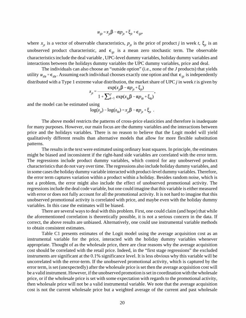
20

where is a vector of observable characteristics, is the price of product j in week t, is anunobserved product characteristic, and is a mean zero stochastic term. The observablecharacteristics include the deal variable , UPC-level dummy variables, holiday dummy variables andinteractions between the holidays dummy variables the UPC dummy variables, price and deal.

The individuals can also choose an “outside option” (i.e., none of the J products) that yieldsutility . Assuming each individual chooses exactly one option and that is independentlydistributed with a Type 1 extreme value distribution, the market share of UPC j in week t is given by

and the model can be estimated using

The above model restricts the patterns of cross-price elasticities and therefore is inadequatefor many purposes. However, our main focus are the dummy variables and the interactions betweenprice and the holidays variables. There is no reason to believe that the Logit model will yieldqualitatively different results than alternative models that allow for more flexible substitutionpatterns.

The results in the text were estimated using ordinary least squares. In principle, the estimatesmight be biased and inconsistent if the right-hand side variables are correlated with the error term.The regressions include product dummy variables, which control for any unobserved productcharacteristics that do not vary over time. The regressions also include holiday dummy variables, andin some cases the holiday dummy variable interacted with product-level dummy variables. Therefore,the error term captures variation within a product within a holiday. Besides random noise, which isnot a problem, the error might also include the effect of unobserved promotional activity. Theregressions include the deal code variable, but one could imagine that this variable is either measuredwith error or does not fully account for all the promotional activity. It is not hard to imagine that thisunobserved promotional activity is correlated with price, and maybe even with the holiday dummyvariables. In this case the estimates will be biased.

There are several ways to deal with this problem. First, one could claim (and hope) that whilethe aforementioned correlation is theoretically possible, it is not a serious concern in the data. Ifcorrect, the above results are unbiased. Alternatively, one could use instrumental variable methodsto obtain consistent estimates.

Table C1 presents estimates of the Logit model using the average acquisition cost as aninstrumental variable for the price, interacted with the holiday dummy variables wheneverappropriate. Thought of as the wholesale price, there are clear reasons why the average acquisitioncost should be correlated with the retail price. Indeed, in the “first stage regressions” the excludedinstruments are significant at the 0.1% significance level. It is less obvious why this variable will beuncorrelated with the error-term. If the unobserved promotional activity, which is captured by theerror term, is set (unexpectedly) after the wholesale price is set then the average acquisition cost willbe a valid instrument. However, if the unobserved promotion is set in coordination with the wholesaleprice, or if the wholesale price is set with some expectation with regards to the promotional activity,then wholesale price will not be a valid instrumental variable. We note that the average acquisitioncost is not the current wholesale price but a weighted average of the current and past wholesale

21

prices. Therefore, we might think that it is less likely to be correlated with the current promotionalactivity.

The columns of Table C1 present results from the same equations as the equivalent columnsin Table 3, computed using two stage least squares. The results are qualitatively very similar to theOLS results in Table 3. In order to address some of the concerns we raised with our instruments, wealso computed similar regressions using the lags of the acquisition costs as instrumental variables.The results were essentially the same. We do not address the potential correlation of deal with theerror term, in any of these cases. We do not feel like we had an appropriate instrumental variable.

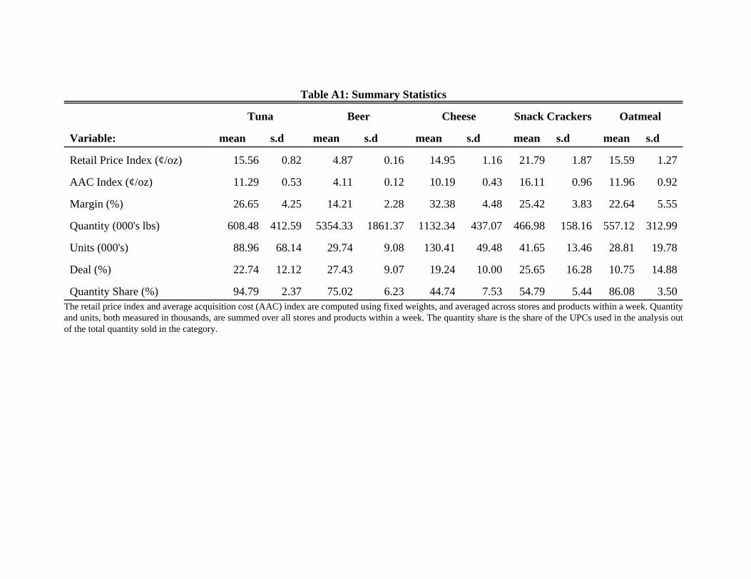
Table A1: Summary Statistics

Tuna Beer Cheese Snack Crackers Oatmeal

Variable: mean s.d mean s.d mean s.d mean s.d mean s.d

Retail Price Index (¢/oz) 15.56 0.82 4.87 0.16 14.95 1.16 21.79 1.87 15.59 1.27

AAC Index (¢/oz) 11.29 0.53 4.11 0.12 10.19 0.43 16.11 0.96 11.96 0.92

Margin (%) 26.65 4.25 14.21 2.28 32.38 4.48 25.42 3.83 22.64 5.55

Quantity (000's lbs) 608.48 412.59 5354.33 1861.37 1132.34 437.07 466.98 158.16 557.12 312.99

Units (000's) 88.96 68.14 29.74 9.08 130.41 49.48 41.65 13.46 28.81 19.78

Deal (%) 22.74 12.12 27.43 9.07 19.24 10.00 25.65 16.28 10.75 14.88

Quantity Share (%) 94.79 2.37 75.02 6.23 44.74 7.53 54.79 5.44 86.08 3.50The retail price index and average acquisition cost (AAC) index are computed using fixed weights, and averaged across stores and products within a week. Quantityand units, both measured in thousands, are summed over all stores and products within a week. The quantity share is the share of the UPCs used in the analysis outof the total quantity sold in the category.

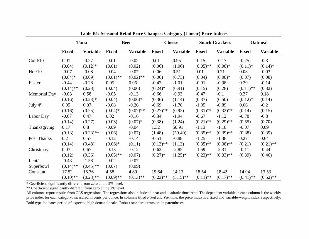
Table B1: Seasonal Retail Price Changes: Category (Linear) Price Indices

Tuna Beer Cheese Snack Crackers Oatmeal

Fixed Variable Fixed Variable Fixed Variable Fixed Variable Fixed Variable

Cold/10

Hot/10

Easter

Memorial Day

July 4th

Labor Day

Thanksgiving

Post Thanks

Christmas

Lent/SuperbowlConstant

0.01(0.04)-0.07(0.04)*-0.44(0.14)**-0.03(0.16)0.05(0.16)-0.07(0.14)0.17(0.13)0.2(0.14)0.07(0.12)-0.43(0.14)**17.52(0.10)**

-0.27(0.12)*-0.08(0.09)-0.28(0.28)0.58(0.23)*0.37(0.25)0.47(0.27)0.8(0.23)**0.57(0.48)0.67(0.36)-1.58(0.45)**16.76(0.23)**

-0.01(0.01)-0.04(0.01)**0.05(0.04)-0.05(0.04)-0.08(0.04)*0.02(0.03)-0.09(0.06)-0.12(0.06)*-0.13(0.05)**-0.02(0.07)4.58(0.09)**

-0.02(0.02)-0.07(0.02)**0.06(0.06)-0.13(0.06)*-0.26(0.07)**-0.16(0.07)*-0.04(0.07)-0.14(0.11)-0.12(0.07)-0.07(0.09)4.89(0.13)**

0.01(0.06)-0.06(0.06)-0.47(0.24)*-0.66(0.36)-0.69(0.27)**-0.34(0.38)1.32(1.48)-0.51(0.13)**-0.62(0.27)*

19.64(0.23)**

0.95(1.06)0.51(0.73)-1.01(0.91)-0.93(1.14)-1.78(0.92)-1.94(1.24)50.91(50.49)-0.88(1.13)-2.85(1.25)*

14.13(5.15)**

-0.15(0.05)**0.01(0.04)-0.01(0.15)-0.47(0.37)-1.05(0.31)**-0.67(0.21)**-1.13(0.35)**-1.25(0.35)**-1.59(0.23)**

18.54(0.11)**

-0.17(0.08)*0.21(0.08)*-0.08(0.28)-0.1(0.50)-0.89(0.32)**-1.12(0.29)**-1.18(0.39)**-1.38(0.38)**-2.31(0.33)**

18.42(0.17)**

-0.25(0.11)*0.08(0.07)0.29(0.11)**0.27(0.12)*0.06(0.14)-0.78(0.55)-0.07(0.38)0.27(0.21)-0.11(0.39)

14.04(0.41)**

-0.3(0.14)*-0.03(0.08)-0.14(0.32)0.18(0.14)-0.2(0.15)-0.8(0.70)0.09(0.39)0.64(0.21)**-0.44(0.46)

13.53(0.52)**

* Coefficient significantly different from zero at the 5% level.** Coefficient significantly different from zero at the 1% level.All columns report results from OLS regressions. The regressions also include a linear and quadratic time trend. The dependent variable in each column is the weeklyprice index for each category, measured in cents per ounce. In columns titled Fixed and Variable, the price index is a fixed and variable-weight index, respectively.Bold type indicates period of expected high demand peaks. Robust standard errors are in parentheses.

Table B2: Seasonal Average Acquisition Cost Changes: Category Price Indices

Tuna Beer Cheese Snack Crackers Oatmeal

Fixed Variable Fixed Variable Fixed Variable Fixed Variable Fixed Variable

Cold/10

Hot/10

Easter

Memorial Day

July 4th

Labor Day

Thanksgiving

Post Thanks

Christmas

Lent/SuperbowlConstant

0.05(0.03)0.04(0.03)-0.02(0.11)0.15(0.13)-0.09(0.09)0.02(0.10)-0.06(0.11)0.03(0.14)-0.03(0.12)-0.20(0.13)12.8(0.09)**

-0.12(0.08)0.04(0.06)0.14(0.17)0.57(0.17)**0.12(0.17)0.42(0.18)*0.44(0.12)**0.35(0.30)0.41(0.22)-1.03(0.40)*12.51(0.16)**

0.00(0.01)-0.02(0.01)**0.04(0.02)0.04(0.02)-0.03(0.03)0.00(0.02)-0.03(0.03)-0.04(0.03)-0.04(0.02)0.02(0.04)3.87(0.06)**

0.00(0.01)-0.03(0.01)**0.04(0.02)0.05(0.03)-0.13(0.05)**-0.09(0.05)0.02(0.03)-0.01(0.04)0.01(0.03)0.06(0.03)3.65(0.08)**

-0.04(0.03)0.00(0.04)-0.45(0.15)**-0.46(0.16)**-0.39(0.13)**-0.09(0.18)0.10(0.14)-0.03(0.12)-0.02(0.10)

13.49(0.09)**

-0.05(0.05)-0.03(0.05)-0.94(0.26)**-0.63(0.24)**-0.66(0.18)**-0.4(0.14)**-0.49(0.41)-0.16(0.15)-0.72(0.17)**

13.28(0.12)**

-0.06(0.03)0.09(0.03)**-0.02(0.12)-0.40(0.24)-0.53(0.14)**0.03(0.10)-0.32(0.12)**-0.36(0.12)**-0.50(0.11)**

14.12(0.07)**

-0.05(0.05)0.28(0.06)**-0.05(0.21)-0.16(0.37)-0.56(0.17)**-0.14(0.20)-0.22(0.15)-0.41(0.18)*-0.79(0.19)**

14.04(0.11)**

-0.14(0.08)0.04(0.05)0.09(0.11)0.01(0.16)0.05(0.14)-0.42(0.41)-0.15(0.41)-0.04(0.46)-0.28(0.30)

12.13(0.35)**

-0.13(0.10)-0.06(0.06)-0.3(0.24)-0.08(0.16)-0.13(0.13)-0.35(0.51)-0.08(0.46)0.09(0.48)-0.64(0.35)

11.52(0.43)**

* Coefficient significantly different from zero at the 5% level.** Coefficient significantly different from zero at the 1% level.All columns report results from OLS regressions. The regressions also include a linear and quadratic time trend. The dependent variable in each column is the weeklyaverage acquisition cost index for each category, measured in cents per ounce. In columns titled Fixed and Variable, the price index is a fixed and variable-weightindex, respectively. Bold type indicates period of expected high demand peaks. Robust standard errors are in parentheses.

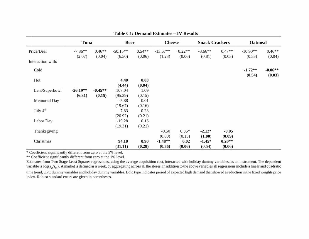
Table C1: Demand Estimates – IV Results

Tuna Beer Cheese Snack Crackers Oatmeal

Price/Deal

Interaction with:

-7.86**(2.07)

0.46**(0.04)

-50.15**(6.50)

0.54**(0.06)

-13.67**(1.23)

0.22**(0.06)

-3.66**(0.81)

0.47**(0.03)

-10.90**(0.53)

0.46**(0.04)

Cold

Hot

Lent/Superbowl

Memorial Day

July 4th

Labor Day

Thanksgiving

Christmas

-26.19**(6.31)

-0.45**(0.15)

4.40(4.44)

107.04(95.39)

-5.88(19.67)

7.83(20.92)-19.28

(19.31)

94.10(31.11)

0.03(0.04)

1.09(0.15)

0.01(0.16)

0.23(0.21)

0.15(0.21)

0.90(0.28)

-0.50(0.80)

-1.48**(0.36)

0.35*(0.15)

0.02(0.06)

-2.12*(1.00)-1.45*(0.54)

-0.05(0.09)

0.20**(0.06)

-1.72**(0.54)

-0.06**(0.03)

* Coefficient significantly different from zero at the 5% level.** Coefficient significantly different from zero at the 1% level.Estimates from Two Stage Least Squares regressions, using the average acquisition cost, interacted with holiday dummy variables, as an instrument. The dependentvariable is . A market is defined as a week, by aggregating across all the stores. In addition to the above variables all regressions include a linear and quadratictime trend, UPC dummy variables and holiday dummy variables. Bold type indicates period of expected high demand that showed a reduction in the fixed weights priceindex. Robust standard errors are given in parentheses.