Why Has Home OwnershipFallen Among the Young?∗

Jonas FisherFederal Reserve Bank of Chicago

jfisher@frbchi.org

Martin GervaisUniversity of Southampton

gervais@soton.ac.uk

September 25, 2008

Preliminary and Incomplete

Abstract

Home ownership of households with “heads” aged 25–44 years peaked in1980. By the 2000 census the rate had fallen by roughly ten percent andit recovered only partially during the 2001–2006 housing boom. The 1980–2000 decline in young home ownership occurred as improvements in mortgageopportunities made it demonstrably easier to purchase a home for the firsttime. This paper uses an equilibrium life cycle model calibrated to micro andmacro evidence to understand why young home ownership fell over a periodwhen it became easier to own a home. We show that, in the presence ofproportional adjustment costs, a trend toward marrying later and the increasein family income risk from delayed marriage, marriage instability, and greaterindividual income risk are sufficient to account for most of the decline in younghome ownership. We explain how changes to taxes, house prices, or householdmobility rates are unlikely to be important factors affecting the decline.

Journal of Economic Literature Classification Numbers: E22; E32; J11; R21Keywords: Housing, home ownership, housing tenure choice, first-time home-

buyers, income risk

∗We are grateful to Faisal Ahmed and Nishat Hasan for research assistance. The views expressedherein are those of the authors and do not necessarily represent those of the Federal Reserve Bankof Chicago or the Federal Reserve System.

1 Introduction

Home ownership of households with “heads” aged 25–44 years peaked in 1980, more

than twenty-five years before the peak of the aggregate home ownership rate in 2006.

By the 2000 census the young home ownership rate had fallen by roughly ten percent

and it recovered only partially during the 2001–2006 housing boom. The 1980–2000

decline in young home ownership occurred as improvements in mortgage opportunities

made it demonstrably easier to purchase a home for the first time. This paper seeks

to understand why home ownership of the young declined so much during a period

when achieving that state became much easier.

Our explanation is driven by trends in marriage and idiosyncratic income risk. We

focus on two trends in marriage since 1980: toward delayed entry into, and greater

exit from, marriage. Individuals are becoming much less likely to be married over the

ages 25–44. Between 1980 and 2000 the marriage rates fell by 15 percentage points

for this age group. The rate of marriage separation (divorced and widowed relative

to all who have ever married at a given age) actually remained stable for ages 25–31,

but for ages 32–44 it rose as much as 8 percentage points between 1980 and 2000.

These two trends mechanically lower the home ownership rate because the married

tend to own more than the unmarried. Indeed applying the 2000 shares of unmarried

and married to the 1980 home ownership rates for these groups accounts for about

50% of the decline young home ownership. Delayed marriage alone does not account

for all of the observed decline because home ownership falls for the married as well.1

The other source of decline in young home ownership is a rise in family income

risk. Increase marriage delay and exit from marriage both increase income risk by

reducing the time spent in the two-worker family state in which risk sharing is possible.

Higher individual income uncertainty should also raise family income risk. There

is a large literature which documents heightened individual and family income risk

after 1980, including Cunha and Heckman (2007), Dynan et al. (2007), Heathcote

et al. (2008), Krueger and Perri (2006) and references therein. Other things equal, an

increase in income risk necessarily lowers home ownership when there are proportional

1Obviously, we are not the first to notice the decline in home ownership of the young or thepotential for marriage to play a role in this decline. See, for example, Haurin et al. (1988) andHaurin et al. (1996).

2

adjustment costs. It is well-known that such costs exist for housing transactions.

In the presence of proportional transactions costs, the option of delaying the home

purchase or sale until the household is possibly wealthier and can afford a larger

house has value. An increase in family income risk increases the value of this option,

thereby increasing delay into home ownership and lowering the home ownership rate.

There are other factors which a priori should work to raise young home ownership

between 1980 and 2000. We have already emphasized innovations in the mortgage

market over our sample period making it easier to buy a house for the first time.

Another important factor is the rise of employment rates for young females after

1980. From 1980 to 1990 the employment rate of 25–44 year old females continued

the increase that began in the early 1960s and rose close to 10 percentage points.

Concurrently, the male-female average wage premium was shrinking. So one- or two-

worker families with at least one female, other things unchanged, are richer, which

can increase young home ownership. Like Caucutt et al. (2002), we suspect that

the increase in economic status of women also drives the two trends in marriage we

emphasize, but we do not model this explicitly.

We disentangle the effects of the competing factors driving young home owner-

ship using an equilibrium life-cycle model of consumption, saving, housing and tenure

choice. The model is calibrated to micro and macro evidence and is consistent with

evidence that income, wealth and marriage are significant predictors of home own-

ership. We use the calibrated model to show that delayed marriage and increased

income risk account for two thirds to four fifths of the decline in home ownership,

after taking into account developments in mortgage and labor markets.

Our paper contributes to an emerging literature that seeks to understand tenure

and housing choices within the context of quantitative equilibrium models. Gervais

(2002) investigates the impact of the preferential tax treatment of houses on tenure

choice. He finds that the effect of mortgage interest deductability on home ownership

is very small compared to the fact that the return to housing equity is not taxed. We

abstract from the preferential tax treatment of housing since, as we argue below, we

do not think it has played a role in the decline in young homeownership. Chambers

et al. (2005) study the rise in home ownership after 1995 within the context of an

equilibrium life-cycle model. They argue that relaxation of borrowing constraints

3

played a big role in this run up. Kiyotaki et al. (2007) study house prices in a model

similar to ours. They investigate factors leading to increases in house prices and the

distributive consequences of this increase. Like us, they find that a relaxation of

the downpayment constraint has only modest implications for housing demand. Dıaz

and Luengo-Prado (2006) examine the determinants of the lifetime pattern of tenure

and housing choices in a life-cycle model with transactions costs. They find that

idiosyncratic earnings uncertainty and a downpayment constraint are key elements of

their quantitative success.

The rest of the paper proceeds as follows. In section 2 we defend our focus on

marriage and income risk in part by arguing that alternative explanations involving

changes to tax policy, house price volatility, or household mobility patterns are un-

likely to account for the decline in young home ownership. In section 3 we describe

our life cycle model and in section 4 we describe our calibration, and demonstrate the

model’s goodness of fit with micro and macro data. Section 5 decomposes the decline

in home ownership of the young into the influence of the various factors we consider.

We conclude in section 6.

2 Motivating Evidence

This section describes the evidence motivating our study. It includes evidence on (i)

the decline in young home ownership during a time when it appears as if first time

buying became easier, (ii) the connection between marriage and home ownership, (iii)

marriage delay and instability, (iv) individual income uncertainty, and (v) why we do

not focus on changes to tax policy, house prices, or household mobility patterns.

2.1 Why Less Ownership if it’s Easier to Own?

Figure 1 displays home ownership rates, defined by the Census Bureau as the number

of households in a category who own divided by all households in that category, for the

economy as a whole and households with designated heads aged 25 to 44 years. These

rates are calculated using the Decennial Census of Housing for the years 1960-2000,

and the American Community Survey for 2006.

4

Figure 1: Home ownership Rates, 1960-2006

.56

.58

.6.6

2.6

4.6

6.6

8

1960 1970 1980 1990 2000 2006Year

All Ages 25−44

Note: These are our estimates using the 1960-2000 DecennialCensus of Housing and the 2006 American Community Survey.

The overall rate grew by 3 percentage points between 1960 and 1980, dipped

by about a percentage point between 1980 and 1990 and rose another 3 percentage

points between 1990 and 2006. Higher ownership rates for older households and an

aging population are the main proximate causes of the post-1990 rise in aggregate

home ownership. For the young the time path is quite different, due to a large drop

between 1980 and 1990 which takes the young home ownership rate two percentage

points below its level in 1960. By 2006 the young ownership rate had recovered less

than a third of the drop between 1980 and 1990.

For concreteness we focus on the years 1980 and 2000. We choose 1980 because

it is the year of the highest young home ownership rates. We use 2000 since by this

time many of the developments that have made it easier to purchase a home have

already occurred, and because the years after 2000 involve seemingly unusual driving

forces which we do not address in this paper.

Table 1 demonstrates that the decline in young home ownership between 1980

and 2000 is broad based. It breaks out the decline in ownership of young households

5

Table 1: Home ownership of the Young by Household Characteristic

Characteristic 1980 2000 Difference

Head’s Age25-44 60.6 57.3 -3.325-29 43.4 36.0 -7.430-34 60.7 53.0 -7.735-39 69.7 63.4 -6.340-44 74.3 69.1 -5.2

Head’s RaceWhite 64.1 63.4 -0.7Black 38.2 36.6 -1.6Other 48.2 41.4 -6.8

Head’s SexMale 67.2 63.9 -3.3Female 36.0 43.1 7.1

Head’s Marital StatusSingle 33.2 38.0 4.8Married 74.5 73.1 -1.4

ChildrenNone 41.4 45.1 3.8One 63.3 60.4 -3.0Two or more 72.5 67.0 -5.5

AdultsOne 30.9 36.2 5.3Two 69.6 66.4 -3.2Three or more 71.7 61.2 -10.5

RegionEast 54.4 53.5 -0.9Midwest 66.4 63.8 -2.6South 62.4 59.1 -3.3West 56.0 50.5 -5.5

Head’s Education< High School 49.8 40.2 -9.5High School or Some College 62.1 57.4 -4.5College 64.8 62.7 -2.1

Head’s Income Quintile1 29.9 27.6 -2.32 45.2 43.0 -2.23 64.3 59.1 -5.24 77.7 73.5 -4.25 86.4 83.9 -2.5

6

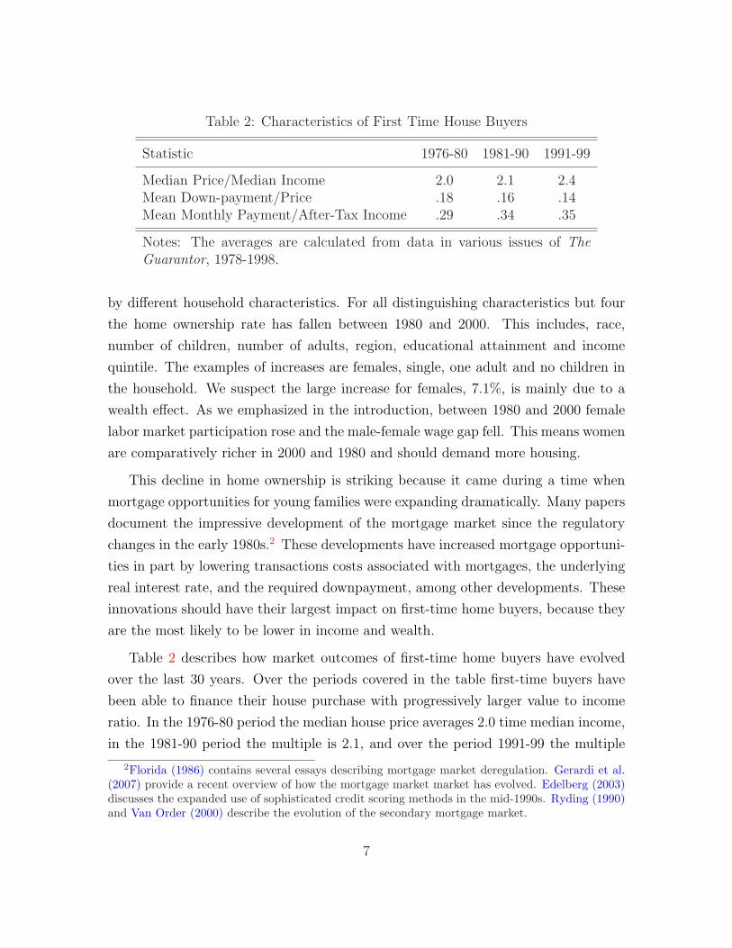
Table 2: Characteristics of First Time House Buyers

Statistic 1976-80 1981-90 1991-99

Median Price/Median Income 2.0 2.1 2.4Mean Down-payment/Price .18 .16 .14Mean Monthly Payment/After-Tax Income .29 .34 .35

Notes: The averages are calculated from data in various issues of TheGuarantor, 1978-1998.

by different household characteristics. For all distinguishing characteristics but four

the home ownership rate has fallen between 1980 and 2000. This includes, race,

number of children, number of adults, region, educational attainment and income

quintile. The examples of increases are females, single, one adult and no children in

the household. We suspect the large increase for females, 7.1%, is mainly due to a

wealth effect. As we emphasized in the introduction, between 1980 and 2000 female

labor market participation rose and the male-female wage gap fell. This means women

are comparatively richer in 2000 and 1980 and should demand more housing.

This decline in home ownership is striking because it came during a time when

mortgage opportunities for young families were expanding dramatically. Many papers

document the impressive development of the mortgage market since the regulatory

changes in the early 1980s.2 These developments have increased mortgage opportuni-

ties in part by lowering transactions costs associated with mortgages, the underlying

real interest rate, and the required downpayment, among other developments. These

innovations should have their largest impact on first-time home buyers, because they

are the most likely to be lower in income and wealth.

Table 2 describes how market outcomes of first-time home buyers have evolved

over the last 30 years. Over the periods covered in the table first-time buyers have

been able to finance their house purchase with progressively larger value to income

ratio. In the 1976-80 period the median house price averages 2.0 time median income,

in the 1981-90 period the multiple is 2.1, and over the period 1991-99 the multiple

2Florida (1986) contains several essays describing mortgage market deregulation. Gerardi et al.(2007) provide a recent overview of how the mortgage market market has evolved. Edelberg (2003)discusses the expanded use of sophisticated credit scoring methods in the mid-1990s. Ryding (1990)and Van Order (2000) describe the evolution of the secondary mortgage market.

7

is 2.4. These more expensive houses are purchased with a down-payment of just 14

percent of the house value on average over the period 1991-99, compared to 16 percent

1n 1981-90 and 18 percent in 1976-80. To acquire the higher value houses relative

to income, first time buyers increase the share of income they devote to mortgage

servicing, rising from .29 in 1976-80 to .35 in 1991-99. Overall, table 2 strongly

suggests it has become easier for first-time home buyers to obtain a mortgage.

2.2 The Connection between Home ownership and Marriage

What drives the housing tenure choice decision? To start our analysis we use the

National Longitudinal Survey of Youth for the 1979 cohort of about 13,000 individuals

14-22 years of age. This is a dataset of individuals but does have information on family

level variables. The sample is 1985-1996 and 1998. With relatively few observations

for individuals aged 40 and over we restrict the sample to those aged 21-39.

We estimate a linear probability model of young home ownership using the vari-

ables in Table 3 plus year effects as regressors. Assets and income are deflated by

the CPI.3 The table displays coefficient estimates with standard errors. The coeffi-

cients on the categorical variables are interpreted as marginal effects on probability

relative to the indicated omitted category. The coefficients on real wealth and assets

are interpreted as the effect of an extra $1000 on the probability of owning. Every

variable is highly significant. Marriage stands out as having a particularly large ef-

fect. The coefficient on marriage says that in our sample if you are married, then

you are 23% more likely to own compared to someone of the same assets, income,

sex, race, education, age, family structure and year who is not married. Other than

wealth and income, only being relatively old and family size come anywhere close to

the importance of marriage as an indicator for home ownership of the young.

The regression results suggest that studying the dynamics of marriage around the

first home purchase could be illuminating. Figure 2 plots conditional probabilities

of being married in the years surrounding a first or second home purchase estimated

3Net assets and income include those for the survey respondent and their spouse, if the spouselives with the respondent. Income is just labor income and net assets includes assets from all sourceslisted in the survey. We use the weights provided by the NLYS in our estimation to correct for theoversampling of the poor and members of the military.

8

Table 3: Linear Probability Model of Young Home ownership

Coefficient Standard Error

Real net assets .006 .0002Real household income .003 .0001Married (versus not married) .23 .005Female (versus male) .01 .003Race is White (versus not white) .02 .004Education is more (versus less) than college -.03 .01Age (versus under 25)

25-29 .04 .00430-34 .09 .0135-39 .14 .01

Adults in household (versus single)2 .013 .004> 3 -.09 .004

Children in household (versus none)1 .05 .0052 .08 .005> 2 .04 .01

Number of Observations 52,233R2 .34

Note: The reported coefficients are from a regression of a dummy variable forhome ownership on wealth, income and dummy variables for the indicatedcategorical variables plus year effects. Standard errors are from using theSTATA linear regression option ‘robust’.

9

Figure 2: Marriage Near Home Purchases

0.1

.2.3

.4.5

Pro

babi

lity

−4 −2 0 2 4Years from purchase

First Second

A. First and Second Purchase

0.1

.2.3

.4.5

Pro

babi

lity

−4 −2 0 2 4Years from purchase

1968−1986 1979−1997

B. 1968 and 1979 Cohorts

Note: These are our estimates from the PSID. They correspondto coefficients from a linear probability model of marriage withdummy variables for each age, year and each number of yearsbefore, during and after the first or second home purchase, plussex, educational attainment and household size. The coefficientscorresponding to -4 to 4 years after the first or second purchaseare plotted with 95% confidence intervals.

using the Panel Study of Income Dynamics. We want to measure the extent to which

marriage is associated with home purchase decisions. We do so by regressing a dummy

variable for whether the respondent is married on a set of dummy variables for the

years before, during and after the first or second purchase, plus dummies for year,

age, household size, educational attainment and sex. The figure plots the fitted values

and 95% confidence intervals for the year relative to year of home purchase dummies.

The omitted category in both cases is individuals who never own.

Figure 2 examines marriage near home purchases using the Panel Study on Income

Dynamics (PSID). Panel A reveals that marriage is more closely associated with the

first home purchase than the second one. In the first purchase case respondents are

approximately 35 percent more likely to be married compared to respondents with

10

the same characteristics but never buy a house. There is a big jump upward in the

likelihood of being married in the year of the first purchase. After the purchase there

is little change in the likelihood of being married. The qualitative pattern of marriage

around the second purchase is similar but much more muted. The peak is about the

same, but there is not the jump at zero which occurs in the first case. We draw two

conclusions from this plot. First, marriage and home purchases occur at similar times.

Second, marriage is more tightly connected to the first purchase than the second.

Figure 2’s panel B illustrates the secular change in the dynamics of marriage and

the first home purchase. Although there is a tight connection between marriage and

the first home purchase in both the 1968-1986 and the 1979-1997 sample periods, the

trend toward later marriages has weakened the relationship. Note that this reduction

is in addition to the secular decline in marriage rates by age which is accounted for

in our regression model by the year dummies. Since individuals purchase homes for

reasons other than family formation, we expect the association between marriage and

the first-purchase to decline if individuals marry later.

Taken together, the regression results strongly suggest that trends in marriage

should be important for understanding the decline in young home ownership.

2.3 Marriage Delay and Instability

We now examing trends in marriage using data from the Decennial Census of Housing.

The first key trend in marriage is that young people are much less likely to be married

at any given age today than they were in 1980. This is demonstrated in Figure 3.

For males, in 1980 there was roughly a 50% chance that you were married at age

25. By 2000 you would have to be 30 years old to have the same chance. Females

behave similarly, but not identically, since the age distribution of matches is different

for males and females.

How should we expect a decline in the marriage rate to affect home ownership?

The answer to this question is in Figure 4. This displays home ownership rates by

marital status for 1980 and 2000. There has been a small increase in home ownership

between 1980 and 2000 for unmarried household heads. This presumably reflects

what we already know from Table 1 that single females have seen a large increase

11

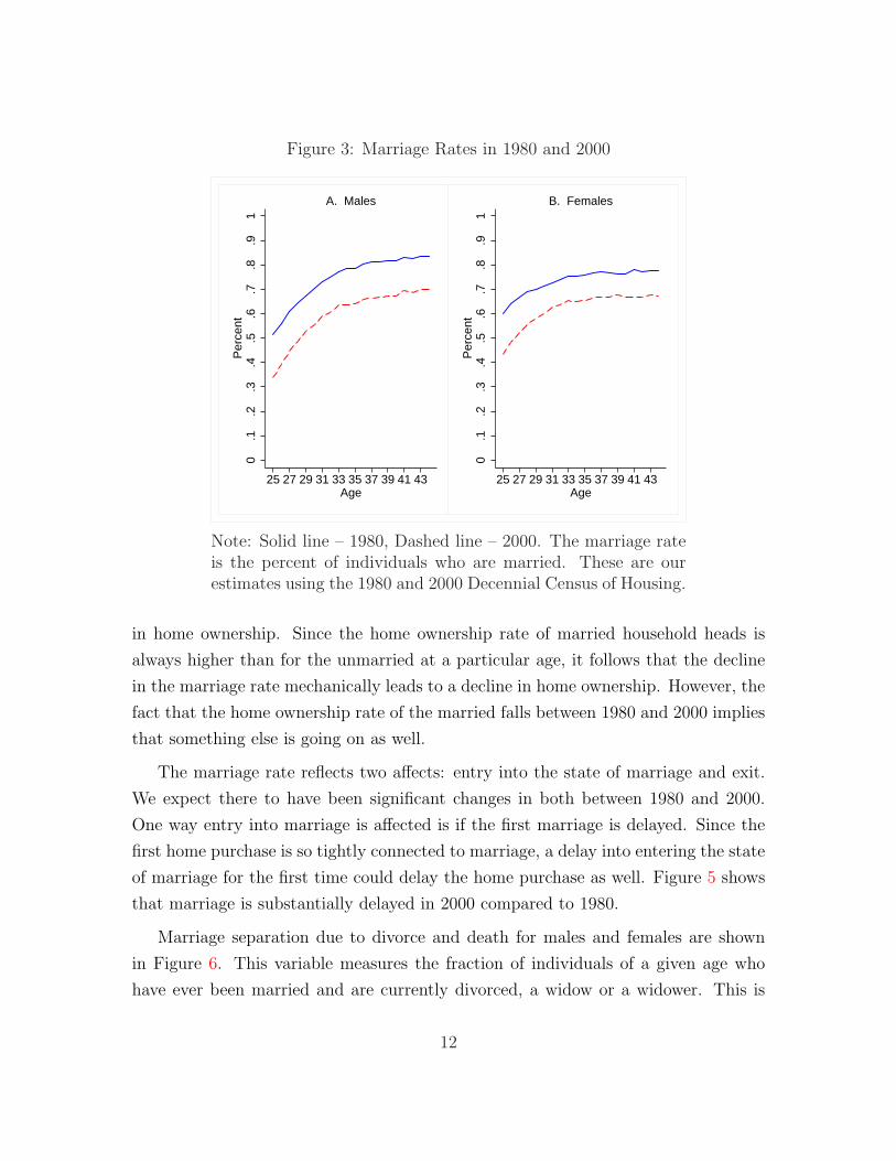
Figure 3: Marriage Rates in 1980 and 2000

0.1

.2.3

.4.5

.6.7

.8.9

1P

erce

nt

25 27 29 31 33 35 37 39 41 43Age

A. Males

0.1

.2.3

.4.5

.6.7

.8.9

1P

erce

nt25 27 29 31 33 35 37 39 41 43

Age

B. Females

Note: Solid line – 1980, Dashed line – 2000. The marriage rateis the percent of individuals who are married. These are ourestimates using the 1980 and 2000 Decennial Census of Housing.

in home ownership. Since the home ownership rate of married household heads is

always higher than for the unmarried at a particular age, it follows that the decline

in the marriage rate mechanically leads to a decline in home ownership. However, the

fact that the home ownership rate of the married falls between 1980 and 2000 implies

that something else is going on as well.

The marriage rate reflects two affects: entry into the state of marriage and exit.

We expect there to have been significant changes in both between 1980 and 2000.

One way entry into marriage is affected is if the first marriage is delayed. Since the

first home purchase is so tightly connected to marriage, a delay into entering the state

of marriage for the first time could delay the home purchase as well. Figure 5 shows

that marriage is substantially delayed in 2000 compared to 1980.

Marriage separation due to divorce and death for males and females are shown

in Figure 6. This variable measures the fraction of individuals of a given age who

have ever been married and are currently divorced, a widow or a widower. This is

12

Figure 4: Home ownership Rates in 1980 and 2000

0.2

.4.6

.81

Per

cent

25 27 29 31 33 35 37 39 41 43Age

A. Unmarried

0.2

.4.6

.81

Per

cent

25 27 29 31 33 35 37 39 41 43Age

B. Married

Note: Solid line – 1980, Dashed line – 2000. The home ownershiprate is the percent of households with a head who owns. Theseare our estimates using the 1980 and 2000 Decennial Census ofHousing.

our measure of the marriage-separation hazard rate. For ages 25-29 there is little

evidence of much change from 1980 and 2000. But there are big differences for ages

30-44. After some period of time a marital pair when assessing the value of the match

may decide that the outside option is best. In 1980 more marriages never reached

this point. Presumably the increases in female employment, educational attainment

and wages have improved the outside option for females significantly so some increase

in the separation rate is to be expected.

2.4 Individual Income Uncertainty

Delayed marriage and marital instability obviously both increase the representative

family’s income risk. Another source of family income risk is individual income risk.

Numerous papers document an increase in cross-sectional variability of both individ-

13

Figure 5: Never Married Rates in 1980 and 2000

0.1

.2.3

.4.5

.6.7

Per

cent

25 27 29 31 33 35 37 39 41 43Age

A. Males

0.1

.2.3

.4.5

.6.7

Per

cent

25 27 29 31 33 35 37 39 41 43Age

B. Females

Note: Solid line – 1980, Dashed line – 2000. The never marriedrate is the percent of individuals who have never married. Theseare our estimates using the 1980 and 2000 Decennial Census ofHousing.

ual and household income over the last three or four decades. Three recent examples

are Cunha and Heckman (2007), Dynan et al. (2007) and Heathcote et al. (2008).

From our perspective, the key finding in the literature is that variability in the cross-

section is higher after 1980 compared to before. The literature disagrees over when

exactly the change occurred, how persistent it has been or whether another change in

variability may have occurred. However there is little disagreement that the answer

to the basic question, “Has individual income risk gone up since 1980?” is “Yes.”

2.5 Fiscal Policy, Home Prices and Household Mobility

We now address some potential alternative explanations for the decline in young

home ownership. These include changes to tax policy, house prices and household

mobility. The key candidate for tax policy is the 1986 tax reform. Poterba (1992) has

14

Figure 6: Marriage Separation Rates in 1980 and 2000

.1.1

5.2

.25

Per

cent

25 27 29 31 33 35 37 39 41 43Age

A. Males

.1.1

5.2

.25

Per

cent

25 27 29 31 33 35 37 39 41 43Age

B. Females

Note: Solid line – 1980, Dashed line – 2000. The marriageseparation rate is the percent of married, divorced or widowedwho are divorced or widowed. These are our estimates using the1980 and 2000 Decennial Census of Housing.

postulated that the reductions in high income marginal tax rates in 1986 lowered the

benefits to the mortgage interest tax deduction, thereby lowering the incentive to own

a home. While there is a direct effect of lowering the top marginal tax rates on the tax

implications of mortgage interest deductability, it is far from clear that this translates

into a substitution from owned to rental housing. Gervais (2002) shows that even

the elimination of mortgage interest deductibility would have modest consequences

for home ownership, especially among high income households. Similarly, Gervais

and Pandey (2008) argue that relatively rich families do not benefit from mortgage

interest deductibility nearly as much as conventionally believed when the family’s

budget constraint is taken into account.4

Should changes in house prices be a consideration in the decline in young home

4The 1996 changes to the tax code effected the amount of capital gains on selling the primaryresidence is exempted from taxes. This should effect the timing of home sales, but we do not thinkit has anything to do with the decline in young home ownership.

15

ownership? If house price volatility went up, then this would increase the value

of delaying a home purchase (or sale). Aggregate measures of house prices do not

suggest that if there has been a trend it is toward less volatility in real house prices,

presumably because the volatility of the consumer price index is lower now compared

to 1980. Moreover Sinai and Souleles (2005) convincingly argue that rent risk is

more important than house price risk in the tenure choice decision. This arises due

to the role of housing as a hedge against variation in rental rates. If rent risk were

to decline, then there would be an incentive to substitute away from owned toward

rented housing. This is an intriguing possibility, but we leave it as an open question

for this paper.

A third possible reason for a decline in ownership is that households’ mobility rates

may have changed. If, for whatever reason, households were to move more frequently,

then, holding all else equal, this should lower home ownership due to the additional

costs involved with moving when a home is owned. As it turns out, mobility reports

by the Census Bureau point toward less, not more mobility. For the young age groups

we study in this paper, the probability that an individual lives at a different address

than in the previous year has fallen from 23% in the mid-1960s to 18% in 2000.5

3 The Model Economy

In this section we describe our life-cycle model. The model consists of households,

goods producing firms, and financial intermediaries. Households derive utility from

consumption and housing services, inelastically supply labor, and via intermediaries

invest in non-residential and housing capital. We assume that owned housing is always

preferred to rental housing of the same size. However, while changing rental housing

is costless, owning requires a downpayment and buying and selling an owner-occupied

house involves transactions costs. We now describe the model in detail.

5This is based on the Current Population Survey findings reported in various issues of “Geo-graphical Mobility” a publication of the Census Bureau.

16

3.1 The Representative Household

Preferences The economy consists of a large number of ex-ante identical house-

holds who forever repeat the same “life cycle” of birth, work, retirement and death.

The transitions between the stages of life occur with fixed and known probabilities.

Households care about their future selves as much as they care about their current

self and so preferences are represented by

Ut = Et

∞∑j=t

βj−tu(cj, ψjhj), 0 < β < 1. (1)

For the incarnation of the household alive in period j, cj denotes the quantity of

goods consumed and hj is the quantity of housing the household occupies and either

rents or owns. The variable ψj determines how much the household prefers to own

rather than rent. When the household rents its home ψj < 1 and when the household

owns its home ψj = 1. The parameter β is the household’s time discount factor. We

assume a time period equals one year. For simplicity, below we drop time subscripts.

With a couple of exceptions, the prime symbol denotes the current value of a choice

variable and the absence of this symbol indicates the previous period’s value of the

same variable.

Stages of the Life-cycle The state variable s controls both the life-cycle status

and labor earnings of a household. Let s ∈ S = Y∪F∪R = {1, 2, . . . , N}∪{N+1, N+

2, . . . , 2N} ∪ {2N + 1, 2N + 2, . . . , 3N}. Households go through three stages of life.

When s ∈ Y , an household is a young type whose housing services when renting are

discounted by ψ(s, 0) = ψy < 1. When s ∈ F , an household is a family type. For this

household type rented housing services are discounted at the rate ψ(s, 0) = ψf < ψy.

We assume the rental discounting is greater for a family household compared to a

young household to capture the empirical phenomenon that, in general, some of the

housing services required by families, such as proximity to good schools and parks,

are hard to obtain in rental housing. Finally, when an household’s state transits to

s ∈ R, the household retires and the rental discount reverts to ψ(s, 0) = ψy.

Non-retired households supply one unit of labor inelastically and face idiosyncratic

uncertainty with respect to their labor productivity. An household in state s ∈ Y ∪F

17

is endowed with e(s) efficiency units of labor, each unit being paid after-tax wage

rate w = (1 − τw)w, where τw is a labor income tax and w is the before-tax wage

rate. The revenues from the labor income tax are used to operate a pay-as-you-go

social security system. All retired households are entitled to a social security payment

equal to a fraction, θ, of average before-tax earnings of the working population. To

keep the notation consistent with working households, we let e(s) = θe/(1 − τw)

if s ∈ R, where e is the average labor productivity of the working-age population.

Given the simple structure of this social security system, it can easily be shown that

τw = θµR/(1− µR), where µR is the fraction of the population that is retired.

The process governing an household’s state over time is described by the Markov

matrix Π,

Π =

ΠYY ΠYF 0N

0N ΠFF ΠFRGΠRY 0N ΠRR

,

where 0N denotes an N ×N matrix of zeros and the other terms are non-zero N ×N

matrices. Since households need to go through an entire life-cycle, the probability of

going from set Y to set R is zero. Similarly, the probabilities of transiting from set Fto set Y and set R to set F are also zero. The elements of matrix ΠYY and those

of matrix ΠFF control how efficiency units supplied by young and family households

evolve over time. The matrices ΠFR and ΠRR are diagonal. The matrix ΠRY controls

the probability of dying and the magnitude of intergenerational income persistence.

We use πss′ to denote individual elements of Π. At the same time as death, a new

generation of households of size G are born, where G > 1 determines the rate at

which the number of households grows.

Labor efficiency of the newborn is controlled by the elements of the matrix ΠRYas follows:

ΠRY =

θ1δ · · · θNδ...

θ1δ · · · θNδ

,

where δ is the probability of dying, and [θ1, . . . , θN ] is the part of the invariant distri-

bution Π associated with the young stage of life. As written, the matrix ΠRY assumes

that there is no intergenerational income persistence because each household has the

same probability of being any of the N types of young households, regardless of the

18

parent’s type at the time of death.

Housing We use the housing tenure variable x′ to indicate whether the household

rents or owns in the current period, and if it owns, the quantity of housing services

consumed. Households who currently own and occupy a house of size hj have x′ = j

and household’s who currently rent have x′ = 0.

Owned houses must be chosen from a finite grid,

G = {hj, j = 1, 2, ..., M : hj ∈ [h, h]}.

Households who rent may choose a continuous quantity of housing for houses smaller

than h, but are confined to the set G for housing larger than h. We discuss below

how h is important for reconciling home ownership rates with the quantity of owned

housing in the economy. We summarize the set of possible house choices in the current

period as follows:

h′ ∈ H(x′), (2)

where

H(x′) =

{(0, h) ∪ G, if x′ = 0;

G, if x′ > 0,

and

x′ ∈ X = {0, 1, 2, ...,M} . (3)

All houses depreciate at the rate δh ∈ [0, 1]. To accommodate the housing grid, we

assume that each house requires a certain amount of maintenance each period in order

to be habitable.

Due to the discounting of rented housing services, without additional assumptions,

households would always choose to own. To motivate an interesting tenure choice we

assume that owning a house involves two kinds of costs. First, we assume that to

own a house the household must have an exogenously determined minimum equity

stake in the house the first year the house is occupied, i.e. it faces a downpayment

constraint. Second, if a household changes the size of its owned and occupied house

it faces costs of buying and selling that are proportional to the size of the house

19

involved. Transactions costs are given by

τ(x, x′) =

τbhx′ , if x = 0 and x′ > 0;

τbhx′ + τshx, if x > 0, x′ > 0 and x 6= x′;

τshx if x > 0 and x′ = 0;

0, otherwise.

Saving Households accumulate wealth with two types of assets: owner-occupied

houses and a generic asset called deposits, d, which pay interest i. We assume the

interest is paid during the current period and the deposit is returned at the beginning

of the next period. Let a denote the household’s net worth at the beginning of the

period. All households face a non-negative savings restriction, a′ ≥ 0. In addition,

homeowners may borrow against their house by acquiring a mortgage at the interest

rate i. Consistent with deposits, the interest is paid during the current period and

the principal is paid at the beginning of the following period. Borrowing against a

home involves a downpayment constraint. This constraint only applies the first year

a house is occupied, that is when the mortgage is first obtained. Once the household

has a mortgage, and as long as the household does not change the size of its house, the

downpayment constraint does not apply. Households are indifferent between paying

down their mortgage and accumulating financial assets. We assume that households

pay down their mortgage before accumulating any financial assets.

The downpayment constraint says that a mortgage acquired in the current period,

m′, is limited to be no more than a fraction γd of the value of the home so that

m′ ≤ (1 − γd)h′. Current savings of an household who chooses to be a homeowner

next period are a′ = d′+h′−m′. It follows that in the year the mortgage is acquired,

savings must be at least as big as the minimum down-payment on the house: a′ ≥ γdh′.

We summarize the constraint on savings as follows

a′ ≥ γ(x, x′), (4)

where

γ(x, x′) =

{0, if x′ = 0 or x′ > 0 and x = x′;

γdhx′ , if x′ > 0 and x 6= x′ .

20

Recursive Formulation of the Household’s Problem The problem faced by

the representative household is to choose sequences of consumption, asset holdings,

housing tenure, and housing services to maximize (1), subject to (2)–(4), c > 0 and

the budget constraint

c + phh′ + a′ + τ(x, x′) = we(s) + a + ia′ (5)

where ph is the price of housing services determined by a no-arbitrage condition

described below.

To address the issue of how to allocate assets of retired households who die between

periods, we introduce annuities. All retired households (the only households who have

a positive probability of dying) pool their net worth together in the current period

and divide that pool among the survivors in the following period according to their

proportion of the pooled net worth. Since each unit of net worth has the same

probability of surviving, 1− δ, each retired ends up with 1/(1− δ) of their net worth

tomorrow should they survive.

Let V (s, x, a) denote the value function of a household who enters a period with

state variables s, x and a. The recursive representation of the household’s problem is

as follows:

V (s, x, a) = max{c>0,x′∈X ,a′≥γ(x,x′),h′∈H(x′)

}

{U(c, ψ(s, x′)h′) + β

∑

s′∈Sπss′V (s′, x′, ϕ(s)a′)

}(6)

subject to (5), where ϕ(s) = 1 unless the household is retired in the current period,

in which case it equals 1/(1− δ).

3.2 Producers

Firms maximize profits

f(k, l)− wl − pkk,

where f(k, l) is a constant returns production function, k denotes non-residential

capital used in production, l denotes the quantity of labor employed, measured in

efficiency units, and pk denotes the rental price of non-residential capital. We assume

21

that producers’ output can be costlessly transformed into consumption goods, and

new residential and non-residential capital. Consequently, the prices of these goods

are all equal to one in a competitive equilibrium. Capital depreciates at the rate

δk ∈ [0, 1].

3.3 Financial Intermediaries

Non-residential investment and investment in rental housing is undertaken by over-

lapping generations of two-period-lived risk neutral financial intermediaries. In their

first period, intermediaries accept deposits from households, Df , which they use to

purchase from the previous generation of intermediaries non-residential capital, Kf

and rental housing capital, Hf , and to issue mortgages to homeowners, M f . During

the period the newly purchased non-residential capital is rented to producers and

the housing is rented to households.6 Interest on deposits is paid at the end of the

first period. At the beginning of the second period, the capital is sold to the new

generation of intermediaries, the mortgage principal is repaid and the deposits are

returned to households. The problem of a new financial institution is:

max{Kf ,Hf

r ,Mf ,Df}(pk − δk)K

f + (pr − δh)Hf + iM f − iDf (7)

subject to the constraint

Kf + Hf + M f ≤ Df , (8)

where φ is a transaction cost of issuing mortgages, which is introduced to permit a

wedge between the borrowing and lending rate for households. The solution to this

maximization problem yields the following no-arbitrage conditions:

pk = i + δk;

pr = i + δh.(9)

It follows that financial institutions are at the margin indifferent between their asset

holdings and liabilities and they make zero profits in equilibrium.

6We assume that new capital is productive immediately, i.e. there is no time-to-build. Thisassumption is made to treat non-residential capital symmetrically with housing. Since a time periodin the model is one year we do not think this assumption is unreasonable.

22

3.4 Stationary Competitive Equilibrium

A stationary competitive equilibrium consists of a value function V (s, x, a), decision

rules for savings ga(s, x, a), tenure choice gx(s, x, a) and housing services gh(s, x, a), an

allocation for financial intermediaries {Df , Kf , Hf ,M f}, aggregate quantities {K ′, H ′, L},prices {i, pr, w, pk}, a fiscal policy {τ, θ}, and a measure λ(s, x, a) such that

1. Given prices and the fiscal policy, the value function and associated policy rules

solve the household problem as given by (6);

2. Given prices and the fiscal policy, producers maximize profits. This implies

factors are paid their marginal products: pk = f1(K′, L), w = f2(K

′, L), where

L is the aggregate demand for labor by producers;

3. Given prices and the fiscal policy, , {Df , Kf , Hf ,M f} solves the financial inter-

mediaries’ problem given by (7) and (8). This implies (8) holds with equality

and the no-arbitrage conditions hold;

4. Aggregates are consistent with individual behavior: λ(s, x, a) is generated by

λ(s′, x′, a′) =

0, if s ∈ R, s′ ∈ Y , a′ > 0∑s∈Y πss′

∑Mx=0

∫a∈A(a′,x′) λ(s, x, da)

+∑

s∈R πss′∑M

x=0

∫a≥0

λ(s, x, da), if s′ ∈ Y , x′ = a′ = 0∑s∈S πss′

∑Mx=0

∫a∈A(a′,x′) λ(s, x, da), otherwise

where

A(a′, x′) = {(a, x) : ga(s, x, a) ≤ a′, gx(s, x, a) = x′};

5. The social security system is self-financed: τw = θµR/(1− µR);

23

6. Markets clear:

Df =∑s∈S

M∑x=0

∫

a≥0

gaλ(s, x, da)−∑s∈S

M∑x=1

∫

a≥0

ghλ(s, x, da)

+∑s∈S

M∑x=0

∫

{a:gh>ga and gx>0}[gh − ga] λ(s, x, da);

H ′ =∑s∈S

M∑x=0

∫

a≥0

ghλ(s, x, da);

Hf =∑s∈S

∫

a≥0

gh(s, 0, a)λ(s, 0, da);

M f =∑s∈S

M∑x=0

∫

{a:gh>ga and gx>0}[gh − ga] λ(s, x, da);

Kf = K ′;

L =2N∑s=1

θse(s).

Here we have suppressed the arguments of the decision rules when there is no

ambiguity about what they are. These expressions are the clearing conditions

for the deposit market, the aggregate housing market, the rental housing mar-

ket, the mortgage market, the non-residential capital market, and the labor

market. These conditions should be transparent except for the deposit market

condition. This condition says all households’ net worth minus total equity in

owner occupied housing must equal deposits at financial intermediaries. If all

these conditions are satisfied then the goods market must clear by Walras’ law.

4 Calibration

We use our model to examine the role of various structural changes on the propensity

to own a home. Our baseline scenario is designed to capture the environment faced

by households in the years leading up to 1980. We compare this baseline scenario

to one which emodies the structural changes which occurred after 1980 and are a

feature of the environment faced by households in the years leading up to 2000. This

section describes how we assign values to the model’s parameters in thee 1980 and

24

2000 calibrations. At the end of this section we briefly discuss household behavior at

the calibrated parameter values.

4.1 1980 Calibration

We assume the functional form of the utility function is

u(c, ψ(s, x)h) = ln(c) +(ψ(s, x)h)1−σh − 1

1− σh

, σh ≥ 0.

and the functional form of the production function is

f(k, l) = Akαl1−α

We set the number of income states to N = 9 and the number of houses to M = 10.

Our results are not sensitive to increasing these values. The upper limits on house

size and assets, h and a are also chosen so that increasing their magnitudes does not

affect our results.

The parameters we need to calibrate include those governing the income process,

{Π, e, θ, τ, G}, preferences, {β, η, σh, ψy, ψf}, the production technology, {α, δh, δk},and housing {h, τb, τs γd}. Our calibration strategy is to first use direct evidence

to assign values to the income and select housing and preference parameters, and

then to choose the remaining housing, technology and preference parameters to bring

the model as close as possible to a short list of aggregate first moments. Table 4

displays parameter values which are held fixed across the 1980 and 2000 calibrations.

Table 5 displays parameters associated with the income process and the downpayment

constraint, some of which change between the two calibrations to account for various

structural changes.

The income process involves three key elements of our analysis. This is where

the speed of transition to “marriage”, differences in income over the life-cycle, and

idiosyncratic risk are determined. We assume that within each of the first two life

stages that income follows a Tauchen and Hussey (1991) approximation to an AR(1)

process. It follows that the income process is completely specified by the mean,

innovation variance and serial correlation of income in the young and family stages

of life, the replacement ratio for the retired life stage, the average duration of each

25

Table 4: Parameters Constant Across the 1980 and 2000 Calibrations

Preferences

β 0.951 σh 3.500 η 0.860

ψy 0.042 ψf 0.100

Housing

τb 0.03 τs 0.06 h 1.15

Production

α 0.257 δk 0.082 δh 0.044

Social Security

θ 0.06 τ 0.061

Table 5: Parameters Governing Differences in the 1980 and 2000 Calibrations

1980 2000

Credit constraint

Minimum downpayment requirement (γd) 0.200 0.133

Income Process

Expected age at transition to family stage 25 27

Expected age at transition to retirement 65 —

Expected lifetime 75 —

Relative mean income of family versus young 1.47 —

Autocorrelation of income 0.95 —

Standard deviation of innovations during young stage 0.025 0.033

Standard deviation of innovations during family stage 0.042 0.056

Productivity effect (A) 1.000 1.041

Population growth 0.020 0.013

Note: No change between calibrations is indicated by “—”.

26

life stage, and the growth rate for the number of households. We now describe how

we calibrate these elements.

We interpret the transition from the young to family type as the event of marriage.

This motivates selecting the duration of the first stage of life so that the fraction of

individuals who do not marry, that is transit to the second stage of life, by age 27,

corresponds to the estimate for the cohort born in the period 1948–1957 reported in

Table IV of Caucutt et al. (2002). Life is assumed to begin at age 18 and we assume

the average durations for the three stages are 7, 37 and 9 years. The length of the

second stage is chosen so that on average people transit to retirement at 65, and the

duration of the retirement stage is chosen so the average life expectancy is 72 years.

Household income jumps significantly around the time of marriage. To capture

this phenomenon we assume that average income of the family type is higher than

for the young type. We calibrate this increase in income by estimating the average

amount by which family income rises upon first marriage using data from the National

Longitudinal Survey of Youth (NLSY).7 We normalize average income over the young

and family stages of life to one and use our estimate of the marriage income increase,

47%, to determine average income in the two stages of life.

The third key feature of the income process involves idiosyncratic risk. This is

governed by the autocorrelation coefficient and innovation variance for the young and

family stages of life. We use the life-cycle income process estimated from the PSID by

Storesletten et al. (2004) to guide our selection of the these parameters. Storesletten

et al. (2004) assume the autocorrelation of income does not change over the working

years of the life-cycle. So, we fix the autocorrelation for the two working life-cycle

stages at a value, .95, which is within the range of estimates reported in Table 2 of

Storesletten et al. (2004). Given the evidence that idiosyncratic risk has risen between

1980 and 2000, we cannot directly use the variance estimates in Storesletten et al.

(2004). Instead, we assume the life-cycle conditional variances they report are an

equally weighted sum of variances from the two halves of their sample, corresponding

7Specifically, we regress percent changes in income on dummy variables for year, age, education,household size, sex and a dummy variable indicating the years before, during and after the year offirst marriage. The estimate for our calibration is the coefficient on the dummy variable for year offirst marriage. The income variable includes earnings income of the individual and, when relevant,their spouse. We describe the NLSY data more in the appendix. We get similar results using thePSID.

27

to our 1980 and 2000 calibrations. Using an assumption, discussed below, on how

much the conditional variances increase, we can calculate estimates of the conditional

variances for both sub-samples. We take the average variance of earnings for the

under 25 and the 26-55 age groups, .3 and .5, to calculate the young and family

cross-sectional variances. Once we have the cross-sectional variances we calulate the

innovation variances using our assumption on the autocorrelation coefficient.

To complete the specification of income, we need to assign values to the social

security replacement ratio, the labor tax and the number of income states in each

of the two working stages of life, and the rate at which the number of households

grows. The replacement ratio for retirees is θ = 0.4, which is taken from Mitchell

and Phillips (2006). We set the labor tax, τ, to the value which finances the social

security system. The number of income stages in each working stage of the life-cycle

is set to N = 9. The growth factor, G is set to 2.35, which corresponds to a growth

rate of 2 percent, which is the mean growth rate of households from 1960-1980 as

reported by the Census Bureau.

The downpayment parameter, γd, is set to .2 in the 1980 calibration. This value

is commonly used in the literature because of its important role empirically. Specifi-

cally, a downpayment of at least 20% is required to avoid paying mortgage insurance.

Housing transactions costs are set to τb = .03 and τs = .06. These values are chosen

as reasonable approximations to actual transactions costs. The main direct evidence

on transactions costs is the percent of the sales price typically charged by realtors and

nominally paid by sellers. This value varies per transaction but the contract rate is

usually near 5%. In practice this value is probably lower since realtors often agree to

cut the fee in order to facilitate a sale. We think it is reasonable to assume that buyers

face transactions costs even though they do not pay the realtor fees directly, since

there are significant search costs involved with buying a house. These considerations

underly our parameter choices here.

The last parameter we fix using direct evidence is the exponent on housing services

in the utility function, σh. We choose this parameter so that our model implies an

income elasticity of housing demand within the range of estimates in the literature,

e.g. Hansen et al. (1998). In particular, we set σh = 3.5. This corresponds to an

income elasticity of demand for housing equal to roughly .35.

28

Table 6: Summary Statistics for the 1980 Calibration

Data Model

Aggregate Ratios

Investment:Output 0.26 0.26

Non-residential Capital:Output 1.95 1.95

Residential capital:Output 0.97 0.99

Owned residential Capital:Total residential capital 0.70 0.65

Housing services:Consumption plus housing services 0.11 0.11

Home-ownership Rates

All households, ages 25–44 0.61 0.60

Never married, ages 25–44 0.25 0.23

Note: The data underlying the empirical statistics are described in the appendix.

The remaining parameters are β, η, ψy, ψf ,, α, δh, δk, and h. The discount rate

β is chosen so that the interest rate in the stationary equilibrium corresponding to

the 1980 calibration is 5%. The remaining five parameters are chosen to minimize

the sum of squared differences between equilibrium values and empirical estimates of

the following variables: the nonresidential plus residential investment to output ratio,

non-residential capital to output ratio, the residential capital to output ratio, the share

of owned residential capital in total residential capital, the share of housing services

in total consumption, the overall home ownership rate of the 25–44 age group and the

home ownership rate of the never married 25–44 age group. The first five moments

are estimated using NIPA data (described in the appendix) for the period 1955–1980.

The second two moments are estimated from the 1980 Census of Housing. Table 6

displays the empirical targets and model implied values for the seven moments. This

table indicates that our model is very good at replicating the aggregate economic

environment circa 1980.8

8Our target for the share of consumption spending that is on housing services is small compared tothat used by some other authors, for example Davis and Ortalo-Magne (2007). Their share is basedon including household operation in housing services and computing it only for renters. Our measureof housing services is based on the NIPA and excludes expenditures on household operations.

29

4.2 2000 Calibration

The 2000 calibration embodies key structural changes that may have influenced home

ownership rates of the young between 1980 and 2000. These include a lower down-

payment constraint, delayed marriage, heightened idiosyncratic income risk, slower

growth in the number of households, and greater aggregate productivity due to the

labor market experience of women.

The downpayment constraint is set to .13, which is 2/3 of the value used in the

1980 calibration. The 2/3 value corresponds to the ratio of the average downpayment

in 1996 to that in 1976 as reported in Table 2. To approximate the phenomenon of

delayed marriage after 1980, we assume that the average duration of the young family

stage is 2 years longer in the 2000 calibration. This implies the same value for the

fraction of individuals who do not marry by age 27 for the cohort born in the period

1958–1967 reported in Table IV of Caucutt et al. (2002), 34%. We set G = 1.83 to

match the rate of growth in the number of households over the period 1980-2000,

1.3%.

The percentage increase in idiosyncratic risk we assume for the later sample is

based on Heathcote et al. (2008). They find the cross-sectional variance of log house-

hold earnings for households headed by males in the 20–59 age group is about 36%

larger in the years leading up to 2000 compared to the years before 1980. This increase

is comparable to other estimates in the literature.

There are two key developments in the labor market experience of women which

may have affected home ownership rates of the young. First, the gender wage premium

has declined substantially. For example, Heathcote et al. (2008) use CPS data to show

that the average wage paid to men relative to women for the period 1967–1980 was

about 1.625 whereas between 1980 and 2000 this ratio averaged about 1.5. Second,

women worked more after 1980. The data compiled by Francis and Ramey (2008)

indicates that average weekly hours worked per female over aged 14 rose from 12.4

for the 1955–1980 period to 17.5 for the 1981–2000 period. In terms of our model,

these changes imply a larger effective supply of labor per household. We model this

as a change in the productivity parameter A from 1 to 1.041.9

9The 4.1% increase in productivity is estimated by calculating the ratio of population shareweighted average weekly pay for males and females in the two sub-samples. The average pay is

30

Figure 7: Housing Decisions in the Model

0.95

1

1.05

1.1

1.15

1.2

0.7

0.75

0.8

0.85

0.9

0 2 4 6 8 10 12 14

1980 Calibration

1980 Calibration with High

Income Risk

4.3 Discussion

Before describing the impact of structural change on the home ownership rates of

the young implied by our 1980 and 2000 calibrations, it is helpful to briefly describe

household behavior in the model. We focus on the role played by income risk. Figure 7

displays the housing service decision rule for low income individuals in the young stage

of life under the 1980 calibration and the 1980 calibration with the level of income

rise set according to the 2000 calibration. On the horizontal access is the beginning

of period level of net worth, a and on the vertical access is the housing choice.

Consider the 1980 calibration case first. This shows that for assets less than about

a = 6 this household chooses to rent. The amount rented rises with wealth. Near

asset level a = 6 the household switches from renting to owning the minimum size

house h1 = h. Due to the discreteness in house sizes and the transactions costs, there

is an interval of assets for which the minimum size house is still chosen. When assets

calculated as follows: for the early sample, .48× 30.28 + .52× 12.42/1.625 and for the later sample,.48× 27.49 + .52× 17.2/1.5. The population shares are from the Census Bureau, the average hoursworked per male and female are from Francis and Ramey (2008), and the relative wages are fromHeathcote et al. (2008).

31

Table 7: Young Home ownership in 1980 and 2000

Data Model

1980 2000 Change 1980 2000 Change

25–29 43.4 36.0 -7.4 47.1 41.8 -5.3

30–34 60.7 53.0 -7.7 59.0 54.3 -4.7

35–39 69.7 63.4 -6.3 67.0 62.6 -4.4

40–44 74.3 69.1 -5.2 72.7 68.4 -4.3

25–44 60.6 57.3 -3.3 59.6 55.3 -4.3

reach a = 12 the household’s desired level of housing services switches to h2. The

step function form of the policy rule continues to the right of a = 12 (there is a very

short flat spot at h2 before the household switches to h3. This basic form of the

decision rule holds for all households in the model. All that changes is the location

of the cut-off values of assets determining when the household selects a different level

of housing services.

The impact of raising income risk (this experiment does confound the general

equilibrium effects of such a change) is to delay switching from renting to owning.

In addition the flat portions of the decision rule are wider. The intuition is straight-

forward. In the presence of proportional adjustment costs there is option value to

delaying the home purchase or sale until you are possibly wealthier and can afford

a larger house. An increase in family income risk increases the value of this option

thereby increasing delay into home ownership. As we will see in the next section, the

aggregate effect of this delay is to lower the home ownership rate.

5 Findings

We now discuss the impact of structural change on the home ownership rates of the

young implied by our 1980 and 2000 calibrations. Table 7 displays home ownership

rates for the age groups of interest in the US data and under the stationary equilibrium

corresponding to each calibration. The empirical values for 1980 and 2000 are taken

from Table 1.

32

It is clear from Table 7 that the model goes a long way to accounting for the

reduction in home ownership rates by age and for the 25–44 category as a whole. The

model implies a larger drop for the 25–44 age group than the data but smaller drops

for the individual age groups. This is because the change in the age distribution in

the model from 1980 to 2000 is not the same as in the data, despite out attempt

to take changes in the rate of household formation into account. By age group our

model accounts for about 2/3–4/5 of the fall in home ownership.

Table 8 sheds light on the factors driving our model’s ability to account for a large

fraction of the decline in young home ownership. This table displays the difference

in home ownership by age for versions of the 1980 calibration where just one of the

five structural changes are imposed. In each case we calculate the home ownership

rates from the corresponding stationary equilibrium. This does not provide a clean

decomposition of the overall effects of structural change due to the general equilibrium

forces at work. Still, we find these experiments informative.

Table 8 indicates that heightened income risk and delayed marriage are the driving

forces behind our findings. These effects lower the home ownership rate substantially

for each age group, the former for the reasons described at the end of the last section

and the latter for the mechanical reason that non-married have lower home ownership

rates compared to married.

The other factor having a large impact is the productivity increase. Recall that

this is our way of modelling the higher wages and work effort of women after 1980.

Not surprisingly this has a large positive impact on home ownership. Still, when all

the structural changes are incorporated, the productivity increase is dominated by

the effects of marriage delay and heightened income risk.

Interestingly lowering the downpayment constraint has a very small positive im-

pact on home ownership. This is despite the fact that the number of “constrained”

home buyers falls from about 10% of those switching from renting to owning to zero.

By “constrained” we mean the fraction of households who switch from renting to

owning who do so with a downpayment exactly equal to the constraint. This small

impact of reducing the rate at which home buyers are constrained is consistent with

Kiyotaki et al. (2007) but stands in contrast to Chambers et al. (2005) who argue

that the reduction in downpayment constraints have a large impact. The reduction in

33

Table 8: Effects of Individual Structural Changes on Young Home ownership

Downpayment Household Income Marriage Productivity

Constraint Formation Risk Delay Increase

25–29 0.01 0.22 -1.82 -2.80 3.59

30–34 0.02 0.15 -2.87 -1.86 3.59

35–39 0.02 0.03 -3.53 -1.09 3.33

40–44 0.02 - 0.08 -3.94 -0.55 3.02

25–44 0.02 0.46 -2.89 -1.67 3.42

the rate of household formation also has a small positive impact on home ownership.

This is due to a general equilibrium effect on the implict rental price of owning. The

lower rate of household growth leads to a greater fraction of wealthier households and

consequently a lower interest rate.

6 Conclusion

Our findings strongly suggest that the decline in home ownership among the young

between 1980 and 2000 is mostly due to a slower rate of marriage formation and

heightened family income risk. According to our model, relaxing the downpayment

constraint on mortgages has a quantitatively small impact on home ownership rates

in the long run. Our findings leave open the possibility that mortgage constraints

may play an important role in cyclical fluctuations.

34

Data Appendix

Data Underlying Estimates of Aggregate Ratios

Except where noted, all expenditure data is from the National Income and ProductAccounts. The capital stock data is from the Bureau of Economic Analysis publication”Fixed Assets and Consumer Durable Goods.”

• Output is measured as GDP plus the service flow of consumer durables obtainedfrom the Federal Reserve Board.

• Non-residential capital includes producer durable equipment and non-residentialstructures, plus the stock of consumer durables and the stock non-residentialgovernment capital.

• Residential capital is the stock of private and public residential capital.

• Owned residential capital is the stock of privately owned residential capital.

• Housing services are the flow of housing services component of consumer expen-diture on services.

• Consumption includes non-housing services plus non-druable expenditures plusgovernment consumption plus the service flow from consumer durables.

35

References

Caucutt, E., N. Guner, and J. Knowles (2002). Why do women wait? Matching,wage inequality, and the incentives for fertility delay. Review of Economic Dynam-ics 5 (4), 815–855.

Chambers, M., C. Garriga, and D. E. Schlagenhauf (2005). Accounting for changesin the homeownership rate. Unpublished manuscript.

Cunha, F. and J. J. Heckman (2007). The evolution of inequality, heterogeneity anduncertainty in labor earnings in the U.S. economy. IZA Discussion Paper No. 3115.

Davis, M. A. and F. Ortalo-Magne (2007). Household expenditures, wages, rents.Unpublished Manuscript.

Dıaz, A. and M. J. Luengo-Prado (2006). On the user cost and homeownership.Unpublished Manuscript.

Dynan, K. E., D. W. Elmendorf, and D. E. Sichel (2007). The evolution of householdincome volatility. Federal Reserve Board, Finance and Economics Discussion SeriesWorking Paper 2007-61.

Edelberg, W. (2003). Risk-based pricing of interest rates in household loan markets.Unpublished manuscript.

Florida, R. L. (Ed.) (1986). Housing and the New Financial Markets. Center forUrban Policy Research.

Francis, N. and V. Ramey (2008). A century of work and leisure. Forthcoming,American Economic Journal: Macroeconomics .

Gerardi, K., H. S. Rosen, and P. Willen (2007). Do households benefit from financialderegulation and innovation? The case of the mortgage market.

Gervais, M. (2002). Housing taxation and capital accumulation. Journal of MonetaryEconomics 49 (7), 1461–1489.

Gervais, M. and M. Pandey (2008). Who cares about mortgage interest deductibility?Canadian Public Policy 34 (1), 1–24.

Hansen, J. L., J. P. Formby, and W. J. Smith (1998). Estimating the income elasticityof demand for housing: A comparison of traditional and Lorenz-concentration curvemethodologies. The Journal of Housing Economics 7, 328–342.

36

Haurin, D. R., P. H. Hendershott, and D. Ling (1988). Home ownership rates ofmarried couples: An econometric investigation. Housing Finance Review 7 (2),85–108.

Haurin, D. R., P. H. Hendershott, and S. M. Wachter (1996). Wealth accumulationand housing choices of young households: An exploratory investigation. Journal ofHousing Research 7 (1), 33–57.

Heathcote, J., F. Perri, and G. L. Violante (2008). Cross-sectional facts for macroe-conomists: United states (1976–2006). New York University manuscript.

Heathcote, J., K. Storesletten, and G. L. Violante (2008). The macroeconomic im-plications of rising wage inequality in the United States. Unpublished manuscript.

Kiyotaki, N., A. Michaelides, and K. Nikolov (2007). Winners and losers in housingmarkets. London School of Economics manuscript.

Krueger, D. and F. Perri (2006). Does income inequality lead to consumption in-equality? Evidence and theory. Review of Economic Studies 73 (1), 163–193.

Mitchell, O. S. and J. W. R. Phillips (2006). Social security replacement rates for al-ternative earnings benchmarks. University of Michigan Retirement Research CenterWP 2006-116.

Poterba, J. M. (1992). Taxation and houisng: Old questions, new answers. AmericanEconomic Review Papers and Proceedings 82 (2).

Ryding, J. (1990). Housing finance and the transmission of monetary policy. FederalReserve Bank of New York Quarterly Review Summer, 42–55.

Sinai, T. and N. S. Souleles (2005). Owner-occupied housing as a hedge against rentrisk. The Quarterly Journal of Economics 120 (2), 763–789.

Storesletten, K., C. I. Telmer, and A. Yaron (2004). Cyclical dynamics in idiosyncraticlabor-market risk. Journal of Political Economy 112 (3), 695–717.

Tauchen, G. and R. Hussey (1991). Quadrature-based methods for obtaining approx-imate solutions to nonlinear asset pricing models. Econometrica 59 (2), 371–396.

Van Order, R. (2000). The U.S. mortgage market: A model of dueling charters.Journal of Housing Research 11 (2), 233–255.

37