RIETI Discussion Paper Series 04-E-016

Why Has the Border Effect in the Japanese Market Declined?

The Role of Business Networks in East Asia

Kyoji Fukao*

Hitotsubashi University and RIETI

Toshihiro Okubo

Graduate Institute of International Studies, Geneva

March, 2004

Abstract

This paper analyzes the causes of the decline in Japan’s border effect by estimating gravity

equations for Japan’s international and interregional trade in four machinery industries (electrical, general,

precision, and transportation machinery). In the estimation, we explicitly take account of firms’ networks.

We find that ownership relations usually enhance trade between two regions (countries), and also find that

we can explain 35% of the decline in Japan’s border effect from 1980 to 1995 in the electrical machinery

industry by the increase of international networks.

JEL Classification numbers: F14; F17; F21;L14

Keywords: Gravity Model; Border Effect; Networks

* Correspondence: Kyoji Fukao, Institute of Economic Research, Hitotsubashi University, Naka 2-1, Kunitachi,

Tokyo 186-8603 JAPAN. Tel.: +81-42-580-8359, Fax.: +81-42-580 -8333, e-mail: k.fukao@srv.cc.hit-u.ac.jp. A

previous version of this paper was presented at the Hitotsubashi Conference on International Trade and FDI,

December 12-14, 2003, Tokyo, Japan. The authors are grateful for the helpful comments by J. Elton Fairfield,

Richard Baldwin, and other conference participants.

1

1. Introduction

As global trade barriers are being steadily dismantled and economies are becoming

increasingly integrated, one would expect international borders to have a diminishing effect on

international trade flows. Nevertheless, economists estimating gravity models to examine trade flows

find that international borders continue to matter. (McCallum (1995), for example, found that trade

between Canada’s different provinces was 22 times as large as trade between the provinces and

different states of the United States.) McCallum’s findings were surprising to those who believed

that trade barriers between Canada and the US did not matter much anymore.

Given that Japan has often been regarded as one of the most closed markets among developed

economies, one would expect to find a large national border effect in the case of Japan.1 Using data

on Japan’s international trade and trade between Japan’s regions, Okubo (2004) found that Japan’s

border effect was smaller than the one estimated for Canada in preceding studies.2 Table 1.1

compares Okubo’s result with Helliwell’s (1998) results on Canada. This table also shows that in

both countries the border effect is declining rapidly. Okubo’s finding is consistent with the casual

observation that Japan has experienced a substantial increase in her import penetration in the 1980s

and 1990s.

INSERT Table 1.1

Probably we can explain the decline in Canadian border effects as the result of trade creation

1 On Japanese trade impediments, see Lawrence (1987), Sazanami, Urata and Kawai (1995), and

Fukao, Kataoka, and Kuno (2003). 2 See McCallum (1995), Helliwell (1996; 1998) and Evans (2000). Using a theoretical model,

Anderson and van Wincoop (2003) recently showed that small-sized countries tend to have smaller

McCallum’s border parameter than large countries. It seems that we can partly explain Okubo’s

result by the relatively large size of the Japanese economy.

2

effects following the launch of NAFTA.3 But what factors caused the decline in Japan’s border

effects? As we shall show later, Japan’s international division of labor with other East Asian

countries has deepened significantly through the fragmentation of production processes and vertical

intra-industry trade. A driving factor behind this trend has been the substantial increase in Japan’s

outward foreign direct investment (FDI) during the 1980s and 1990s, spurring Japan’s international

trade and contributing to the decline in the border effect.4

A number of studies have analyzed the relationship between Japan’s FDI and the increase in

her international trade. Using industry level data on Japan’s international trade and on exports and

imports by Japanese firms’ foreign affiliates, Fukao and Chung (1997) showed that since around

1986 Japan’s FDI in Asia has contributed to re-imports5 and intermediate goods trade.6 Fukao,

Ishido and Ito (2003) examined the influence of Japan’s FDI on its VIIT more rigorously: they

developed a model to capture the main determinants of VIIT that explicitly includes the role of FDI

then tested this model empirically, using data from the electrical machinery industry. Their findings

show that FDI does play a significant role in the rapid increase in VIIT in East Asia seen in recent

years. But few empirical studies on this issue have measured how Japan’s FDI has reduced national

border effects.7

3 On the Canadian case, see Fairfield (2003). 4 Another possible explanation for the decline of the border effect is that reductions in Japan’s tariff

rates and non-tariff barriers have increased Japan’s foreign trade. But reductions in Japan’s tariff

rates mainly occurred in the period of 1960-1980; Japan’s average tariff rate was already very low in

the 1980s (Okubo 2004). In the case of Japan’s machinery industry, it seems that, by the 1980s,

non-tariff barriers were also not particularly high (Sazanami, Urata, and Kawai 1995 and Fukao,

Kataoka, and Kuno 2003). 5 Re-imports are defined as Japanese foreign affiliates’ exports to Japan. 6 On this issue, also see Lipsey, Ramstetter, and Blomström (1999). 7 One study examining the relationship between Japan’s outward FDI and imports using a gravity

type equation is the one by Eaton and Tamura (1994), which, however, does so only at the macro

3

The aim of this paper is to study the causes of the decline in Japan’s border effect by

estimating gravity equations for Japan’s interregional trade and trade between Japan’s regions. In the

estimation, we explicitly take account of interfirm networks. We conduct separate gravity model

estimations for four machinery industries (electrical, general, precision, and transportation

machinery). Our reasons for focusing on these four sectors are as follows: (a) most of Japan’s FDI in

the manufacturing sector has been concentrated in the machinery industry; and (b) even within the

machinery industry, there are large differences in the patterns of VIIT and outsourcing in the

electrical machinery and the transportation machinery sector, as we will show in the next section. In

order to analyze the effects of interfirm networks on international trade, it is necessary to look at

trade flows at a relatively disaggregated level.

It is important to note the that national border effects estimated in a gravity equation will

depend not only on outward FDI, but also on inward FDI and firms’ networks linking Japan’s

regions. Using inward FDI statistics and data from the Establishment and Enterprise Census, we will

take these factors into account.

The remainder of the paper is organized as follows. Section 2 provides an overview of Japan’s

trade and FDI patterns; Section 3 presents an econometric analysis of Japan’s border effects; and.

Section 4 summarizes the main findings of this paper.

2. Overview of Japan’s International Trade

In this section, we take a general look at the pattern of Japan’s trade and FDI in the last two

decades.

2.1 Rapid Increase in the Import Penetration of Manufactured Products

level.

4

Although Japan’s overall import-GDP ratio gradually declined over the last two decades,

imports of manufactured products have actually grown faster than the economy as a whole (Table

2.1).8 As Figure 2.1.B shows, the increase in imports is mainly concentrated in electrical machinery

and labor intensive goods, such as apparel and wooden products, which in this figure are classified

as “other manufacturing products.” Since the share of the manufacturing sector in GDP declined

during this period, the ratio of imports of manufactured products to gross value added in the

manufacturing sector increased rapidly: by 11.5 percentage-points from 15.2% in 1985 to 26.7% in

2000 (Table 2.1).9

INSERT Table 2.1 and Figure 2.1

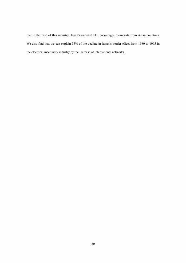
In contrast with the rapid changes in the commodity composition of Japan’s imports, the

commodity composition of Japan’s exports has remained relatively stable over the last fifteen years

(Figure 2.1.A).

Japan’s increased imports of electrical machinery and labor intensive products are mainly

provided by East Asian economies. Figure 2.2 shows that nine East Asian economies (China, Hong

Kong, Taiwan, Korea, Singapore, Indonesia, Thailand, the Philippines, and Malaysia) provided

64.2% of Japan’s electrical machinery imports and 49.2% of Japan’s imports of “other

manufacturing products” in 2000. The East Asian economies’ share in Japan’s total imports of

machinery and intermediate products such as metal products and chemical products has also

8 Comparing export shares and import penetration in the US, Canada, the UK and Japan during the

period 1974–93, Campa and Goldberg (1997) found import penetration to be extremely stable and

significantly lower in Japan than in the other countries. However, Japan has experienced a

substantial change in her import penetration in the 1990s. If we were to conduct a similar analysis

using more recent data, it seems probable that Campa and Goldberg’s conclusion no longer holds. 9 The United States experienced a similar trend during the 1980s, when this ratio jumped by 12.4

percentage-points from 18.3% in 1978 to 30.7% in 1990 (Sachs and Shatz 1994).

5

increased rapidly.

INSERT Figure 2.2

As a result of these trends, East Asia during the 1990s became the most important destination

for and origin of Japan’s international trade. As Figure 2.3 shows, trade with the nine East Asian

economies accounted for 48.5% of Japan’s total manufactured imports and 41.0% of total

manufactured exports in 2000.

INSERT Figure 2.3

2.2 Fragmentation and Vertical Intra-industry Trade

This rise in Japan’s imports of labor intensive products and exports of capital and technology

intensive products (such as machinery and advanced intermediate products) can be easily recognized

as a deepening of the international division of labor with the relatively unskilled-labor abundant East

Asian economies. But how can we interpret the rapid increase in the two-way trade in electrical

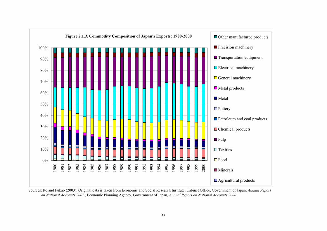
machinery? Table 2.2, presenting Japan’s bilateral trade in electrical machinery with China and Hong

Kong in 1999 at the 3-digit level, provides a clue.

INSERT Table 2.2

This table shows two important facts. First, there is a huge trade in electrical machinery

equipment and related parts and components between Japan and China plus Hong Kong. According

to MITI (1999), the share of machine parts in Japan’s total exports to East Asia increased from

31.7% in 1990 to 40.2% in 1998. It seems that the international division of labor through the

fragmentation of production processes has contributed to the increase of Japan’s trade with East

Asia.

The second important fact that this table shows is the existence of huge intra-industry trade

between Japan and China plus Hong Kong. For example, in the case of television receivers, the total

trade value is 37 times greater than the trade balance.

6

Using Japan’s custom statistics on electrical machinery trade at the HS 9-digit commodity

classification (Harmonized Commodity Description and Coding System), Fukao, Ishido and Ito

(2003) found that in the case of Japan’s trade with East Asian economies, the unit prices of Japan’s

exports tends to be substantially higher than those of her imports. On the assumption that the gap

between the unit value of imports and the unit value of exports for each commodity reveals the

qualitative differences of the products exported and imported between the two economies, their

findings indicate that there has been a rapid increase in Japan’s intra-industry trade with a vertical

division of labor, i.e. vertical intra-industry trade (VIIT), with her East Asian neighbors.10 Figure 2.4

shows the share of the trade types for Japan’s trade in the electrical machinery industry by partner

region or economy in 1988, 1994 and 2000. This figure is a simplex diagram, where a set of shares

of the three trade types is expressed as one point in the diagram. The distance between this point and

the horizontal line HIIT-VIIT denotes the share of one way trade (OWT). Similarly, the distance to

the line OWT-VIIT denotes the share of horizontal intra-industry trade (HIIT), while the distance to

HIIT-OWT denotes the share of vertical intra-industry trade (VVIT). For the definition of the three

trade types see Appendix A. The starting point of each arrow corresponds to the value for the year

1988 and the end of the arrow corresponds to the value for 2000. This figure reveals a dramatic

increase of VIIT in Japan’s trade with China and the ASEAN countries during 1988 to 2000.

INSERT Figure 2.4

The contribution of VIIT to the rapid increase in intra-regional trade in East Asia is shown by

a comparison of intra-regional trade pattern in East Asia and the EU.

The simplex diagrams in Figures 2.5 and 2.6 show the shares of the three trade types in

10 Major preceding studies on vertical intra-industry trade using this gap between unit export and

import prices to distinguish vertical and horizontal IIT are Greenaway, Hine, and Milner (1995),

Fontagné, Freudenberg, and Péridy (1997), and Aturupane, Djankov, and Hoekman (1999).

7

intra-EU and intra-East Asian trade for each commodity category.11 The starting point of each arrow

corresponds to the value for the year 1996 and the end of the arrow corresponds to the value for

2000. Although the figures for East Asia are located towards the upper right in comparison with

those for the EU, there is a similar pattern in terms of the differences between commodity groups. In

both regions, OWT dominates in agricultural and mining products. The share of VIIT is relatively

high in the trade in machinery.

INSERT Figure 2.5 and 2.6

There also exist some differences between trade in the EU and in East Asia. In East Asia, the

share of VIIT is exceptionally high in electrical machinery and general and precision machinery.

We should note that in East Asia, export oriented FDI is concentrated in these sectors. In the EU, the

shares of VIIT and HIIT are very high not only in the trade in this type of machinery but also in the

trade in many other manufacturing products, such as chemical products, transportation machinery,

and wood and paper products.

It is important to note that the commodity composition of intra-East Asian trade is very

different from that of intra-EU trade, which as is shown in Figures 2.7 and 2.8. In East Asian trade,

the shares of electrical machinery and general and precision machinery are very high (30.5% and

19.2% respectively versus 10.7% and 18.1% for the EU), while the shares of transportation

machinery and chemical products are very low in comparison with the EU (2.3% and 9.0% versus

16.0% and 15.5%).These differences and the fact that the IIT shares are very high in the EU trade in

transportation machinery and chemical products seem to imply that IIT has contributed to the

increase in trade volumes in both regions. IIT has been a crucial factor underlying the overall

11 For the analysis of trade patterns in the EU and East Asia, Fukao, Ishido and Ito (2003) used the

PC-TAS (Personal Computer Trade Analysis System) published by the United Nations Statistical

Division. The dataset is based on the 6-digit HS88 commodity classification.

8

increase in trade.

INSERT Figure 2.7 and 2.8

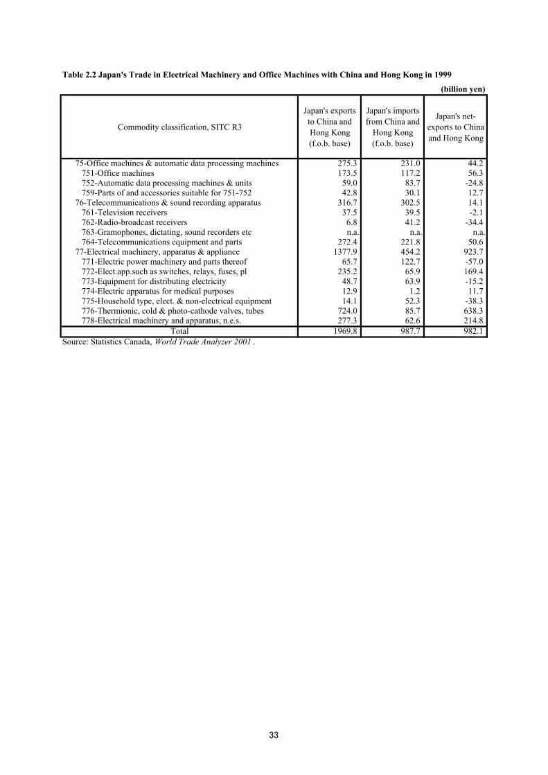
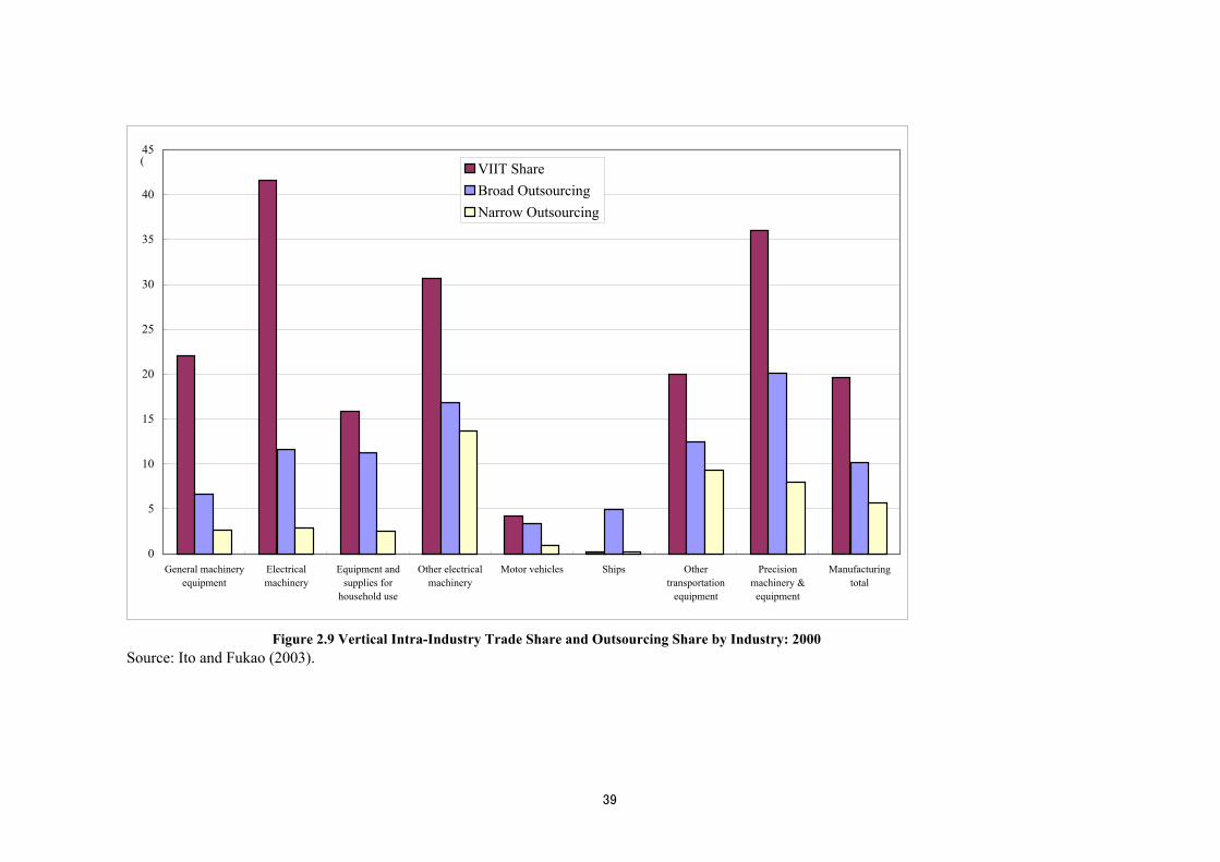
Ito and Fukao (2003) showed that, Japan’s transportation machinery industry is lagging behind

other machinery industries not only in VIIT but also in outsourcing. Figure 2.9 shows the share of

VIIT and outsourcing measures derived by Ito and Fukao (2003). Their measures of broad and

narrow outsourcing are constructed following Feenstra and Hanson (1999).12 The broad outsourcing

measure expresses imported intermediate inputs relative to total expenditure on non-energy

intermediate inputs in each industry.13 The narrow outsourcing measure represents the imported

intermediate inputs from the same industry as the good being produced (based on the Japan

Industrial Productivity [JIP] database) divided by the total expenditure on non-energy intermediate

inputs in each industry.14 Ito and Fukao’s (2003) finding that Japan’s transportation machinery

industry is behind in VIIT and outsourcing is consistent with our previous finding that the trade

share of transportation machinery in East Asian total trade is much smaller than in the EU.

INSERT Figures 2.9 and 2.10

Figure 2.10 presents the growth rate of the VIIT share and the growth rates of the broad and

narrow outsourcing measures for the period 1988–2000 for each industry. This shows that all three

measures have increased in all the machinery industries except in the ship building industry. The

broad and narrow outsourcing measures have grown more rapidly than the VIIT share in almost all

the industries.

2.3 The Role of Foreign Direct Investment

12 For the definition of broad and narrow outsourcing measures, see Appendix A. 13 Ito and Fukao’s (2003) industry classification is based on the basic industry classification of the

Japan Input-Output Tables 1990 by the Management and Coordination Agency. Their classification

lists 246 manufacturing industries 14 The JIP database classifies the manufacturing sector into 35 industries.

9

It is important to note that Japan’s foreign direct investment (FDI) plays a key role in the rapid

growth of Japan’s trade in manufactured products with the rest of East Asia. Table 2.3 shows the

share of Japan’s trade with Japanese affiliates abroad in Japan’s total trade with East Asia in 1999.

Both imports of intermediate products from Japan by Japanese manufacturing affiliates in East Asia

and exports of their output to Japan occupy a large share in Japan’s total trade with this region.

Though in the case of general machinery, the share of procurements by Japanese manufacturing

affiliates’ located in East Asia in Japan’s total exports to East Asia does not seem to be large, it is

important to note that this share does not include Japanese affiliates’ purchases of investment goods

from Japan. Japanese affiliates in East Asia imported 400 billion yen worth of capital equipment for

investment from Japan in 1999. Probably a substantial part of the equipment imports consists of

general machinery.15

Figure 2.11 shows the trade and FDI patterns for Japan’s machinery industry. In the case of the

two leading export industries, electrical machinery and transportation machinery, production by

Japanese affiliates abroad surpassed exports from Japan. Especially in the case of electrical

machinery, Japan’s imports have increased rapidly. As we have seen in Table 2.3, one half of Japan’s

imports from East Asia are produced by Japanese affiliates there.

INSERT Table 2.3 and Figure 2.11

Fukao, Ishido and Ito (2003) examined the influence of Japan’s FDI on its VIIT more

rigorously: they developed a theoretical model to capture the main determinants of VIIT that

explicitly includes the role of FDI and then tested this model empirically, using data from the

15 Japan’s total exports of general machinery to East Asia amounted to 1,200 billion yen in 1999.

Okubo (2003b) analyzed Japan's IIT in recent years, finding that not only a similarity of GDP levels

but also technological similarity across nations enhance IIT, and that Japanese FDI toward Asian

countries greatly contributes to such technological similarity.

10

electrical machinery industry. The findings show that FDI does indeed play a significant role in the

rapid increase in VIIT in East Asia seen in recent years.

3 Econometric Analysis

In this section we conduct a statistical analysis of border effects for Japan’s international trade

and trade among Japan’s regions and study how Japanese firms’ networks across countries and

regions have influenced Japan’s trade pattern.

3. 1 Data and Methodology

The majority of studies on border effects so far has been based on the estimation of gravity equations

at the macro level (McCallum 1995, Helliwell 1996, 1998, Evans 2000, Anderson and van Wincoop

2003, and Okubo 2003a ). In this paper, we conduct estimations of a gravity model for four

machinery industries (electrical, general, precision, and transportation machinery).16

Studies estimating gravity equations at the macro level have used the GDP of the exporting

country (or region) as the measure of production and the GDP of the importing country (or region)

as the measure of the size of demand. For our industry-level analysis, we use domestic production

and domestic demand in each industry in place of GDP.17 We obtain regional domestic demand and

production data from the Input-Output Tables of Interregional Relations (Chiiki-kan Sangyo Renkan

Hyo) published by the Ministry of Economy Trade and Industry (MITI), which are published every

16 It is also important to note that machinery products are usually well differentiated and this

characteristic is consistent with basic assumptions in the standard gravity model. 17 Helliwell (1998, Ch. 2) estimated gravity equations at the industry level. He used the GDP of

exporting and importing provinces (or states). He observed positive and significant border effects at

an industrial level between Canada and the United States. We think that his approach is problematic

because the regional distribution of production of certain industries is usually quite different from

the distribution of GDP and, similarly, the distribution of domestic demand for a certain industry is

not identical with the distribution of GDP.

11

five years and cover all the industries at the 2-digit level divided into nine Japanese regions:

Hokkaido, Tohoku, Kanto, Chubu, Kinki, Chugoku, Shikoku, Kyushu, and Okinawa. Since

Okinawa’s economy is very small in comparison with the other regions and the production of

machinery in Okinawa is negligible, we excluded Okinawa from our data and analyzed eight

regions.

We obtain cross country data of domestic demand and production from the Industrial Demand

Supply Balance Database of the United Nations Industrial Development Organization (UNIDO).

The UNIDO data are available from 1981; based on the five-year intervals dictated by the regional

I-O tables, our econometric analysis therefore begins in 1980 (where we use 1981 data for 1980).

The drawback of our source for data on interregional trade in Japan is that the international

trade data in the I–O table are available only at the national level. There are no statistics on each

region’s bilateral trade with other countries. Therefore, we had to estimate this data, using the

following methodology: first, we calculated each region’s share in Japan’s total imports and exports

for each industry in I-O table. Next, we multiplied Japan’s bilateral international trade in each

industry with each region’s trade share. We obtain data on Japan’s international trade from the World

Trade Flows 1980–1997 of the Center for International Data, University of California, Davis. Figure

3.1 shows the share of international trade in the total trade of the eight Japanese regions for each

industry. The denominator of each value is the sum of the eight regions’ imports from (exports to) all

foreign countries and all the other regions. The numerator is the sum of the eight regions’ imports

from (exports to) all the foreign countries. The share of international imports in total imports of the

eight regions increased in all the four industries in 1980–1995 and was especially large in the

electrical and the precision machinery industries. In contrast, the share of international exports in

total exports of the eight regions declined slightly in the transportation and the precision machinery

industries.

12

INSERT Figure 3.1

Foreign countries’ GDP was taken from the World Bank’s World Development Indicators,

while the GDP of the eight Japanese regions is from the Prefectural Income Statistics (Kenmin

Shotoku Tokei) by the Ministry of Public Management, Home Affairs, Posts and

Telecommunications.

We measure the size of Japanese firms’ networks in a certain industry, which connect Japan

with the same industry in a foreign country, by the number of Japanese affiliates in the same industry

in that country. We measure the extent of Japan’s international links in a particular industry by using

the number of Japanese affiliates in that industry in a particular country. Similarly, we measure

foreign countries’ network links with Japan in a particular industry by using the number of those

countries’ affiliates in Japan in the same industry.

We obtain these data from various issues of the following MITI publications: the Basic

Survey of Overseas Business Activities (Kaigai Jigyo Katsudo Kihon Chosa), the Survey on Trends of

Japan’s Business Activities Abroad (Kaigai Jigyo Katsudo Doko Chosa) and the Report on Trends of

Business Activities by Japanese Subsidiaries of Foreign Firms (Gaishi-kei Kigyo no Doko). No

statistics on Japan’s region’s bilateral inward and outward direct investment relationship with other

foreign countries at the industry level are available. We assume that Japan’s inward and outward FDI

affects all Japanese regions in a similar way and use national data on FDI for each region. Figure 3.2

shows firms’ network linkages between Japan and foreign countries. The number of foreign affiliates

owned by Japanese firms increased very rapidly in 1980–1995. In contrast, the number of foreign

firms’ affiliates in Japan stagnated.

We measure the size of firms’ networks in a certain industry in region i, which connect this

region with the same industry in region j, by the number of establishments owned by firms in region

i and located in region j. We take this data from the Special Aggregation Tables of the Establishment

13

and Enterprise Census (Jigyosho Kigyo Tokei Chosa, Tokubetsu Shukei Hyo) of the Ministry of

Public Management, Home Affairs, Posts and Telecommunications. Unfortunately, the data are

available only for 1991. We assume that firms’ interregional networks in Japan remained unchanged

during the period 1980–1995 and use the same data for this period.18

3.2 The Empirical Model

First we estimate a McCallum-type gravity equation for each industry (McCallum 1995):

log(TRADEi, j, tk) = α0 + α1log(GDPi, t) +α2log(GDP j, t) + α3log(DISi, j)

+α4GAPi, j, t + ∑=

95

80τ

α5τBORDUMi, j*YEARDUMt, τ + εi, j, tk (3.1)

where TRADEi, j, tk denotes the nominal exports (in million yen) of industry k products from country

(or region) i to country (or region) j in year t. We use data of cross-regional trade within Japan (i∈R

and j∈R, where R denotes the set of the eight Japanese regions) and data of Japan’s international

trade (i∈R and j∈C, or i∈C and j∈R, where C denotes the set of Japan’s trade partner countries) for

the years 1980, 1985, 1990, and 1995. GDPi, t and GDPj, t are the gross domestic products in country

(or region) i and country (or region) j in year t. DISi, j is the distance (in km) between the capital (or

the seat of government of the prefecture with the largest GDP in the region) of country (region) i and

the capital (or the seat of government) of country (region) j.19 GAPi,j,t denotes the absolute value of

the difference of the logarithm of the per-capita GDP of i and the logarithm of the per-capita GDP of

j in year t. BORDUMi,j is a dummy variable for domestic trade. BORDUMi,j =1, if i∈R and j∈R.

18 According to various issues of the Establishment and Enterprise Census, the number of

manufacturing establishments in the years 1981, 1986, 1991, and 1996 was 873,000, 875,000,

857,000, and 772,000 respectively. Therefore, it seems that the number of firms’ interregional

linkages in Japan have stagnated or slightly declined in the period. On this issue, see Tomiura

(2003). 19 To calculate the distance between a region in Japan and a foreign country, we used the distance

between Tokyo and the capital of the foreign country.

14

Otherwise BORDUMi,j =0. YEARDUMt,τ is a year dummy. YEARDUMt,τ=1 if τ=t. Otherwise

YEARDUMt,τ=0. εi, j, tk is an ordinary error term. In order to take account of the possibility of

heteroscedasticity among different groups, we estimate this and the following equations by the

feasible generalized least square (FGLS) method.

Next, we estimate an equation in which we replace the GDP of exporting country (region) i

with SUPEXi, tk – representing the total domestic supply of industry k output in country (region) i –

and the GDP of the importing country (region) j with DEMIM j, tk – which stands for the total

domestic demand for industry k output in country (or region) j:

log(TRADEi, j, tk) = α0 + α1log(SUPEXi, t

k) +α2log(DEMIM j, tk) + α3log(DISi, j)

+α4GAPi, j, t +∑=

95

80τ

α5τBORDUMi, j*YEARDUMt, τ+ ∑=

95

80τ

α6τ EXDUMi, j *YEARDUMt, τ + εi, j, tk

(3.2)

The border effect on imports might be different from the border effect on exports. In order to control

for this difference, we add an export dummy EXDUMi, j on the right hand side. EXDUMi, j=1, if i∈R

and j∈C. Otherwise EXDUMi, j=0.

In the third equation, we add network variables:

log(TRADEi, j, tk) = α0 + α1log(SUPEXi, j, t

k) +α2log(DEMIMi, j, tk) + α3log(DISi, j)

+α4GAPi, j, t +∑=

95

80τ

α5τBORDUMi, j*YEARDUMt, τ +∑=

95

80τ

α6τ EXDUMi, j *YEARDUMt, τ

+α7log(NPAAFWOi, j, tk) +α8log(NAFPAWOi, j, t

k) +α9log(NPAAFJAi, jk) +α10log(NPAAFJAi, j

k)

+ εi, j, tk (3.3)

where NPAAFWOi, j, tk and NAFPAWOi, j, t

k denote variables for networks between Japan and the

foreign country. NPAAFWOi, j, tk denotes the number of cross-border ownership relations in year t in

industry k where the parent firm is located in exporting country (region) i and the affiliate is located

in importing country (region) j. Conversely, NAFPAWOi, j, tk denotes the number of cross-border

15

ownership relations in year t in industry k where the parent firm is located in the importing country

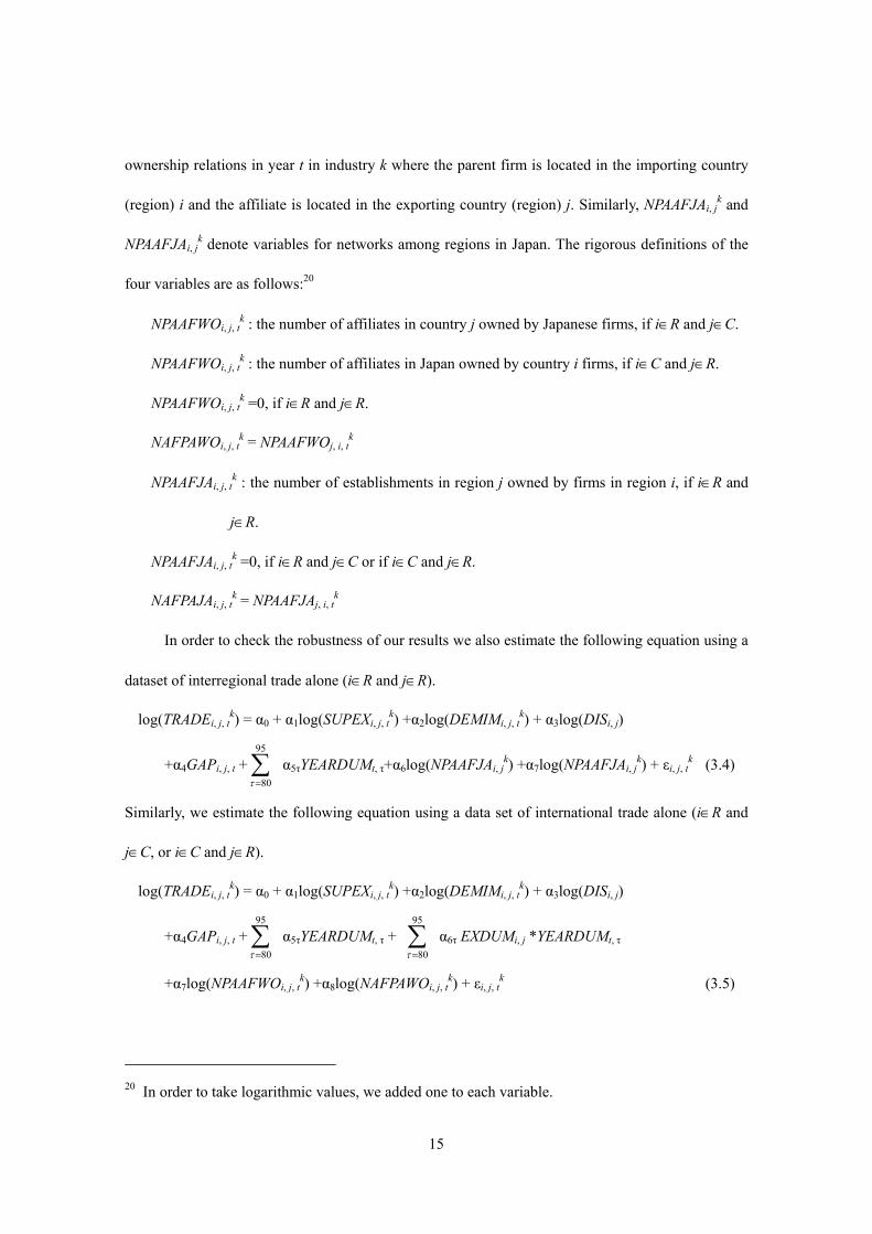
(region) i and the affiliate is located in the exporting country (region) j. Similarly, NPAAFJAi, jk and

NPAAFJAi, jk denote variables for networks among regions in Japan. The rigorous definitions of the

four variables are as follows:20

NPAAFWOi, j, tk : the number of affiliates in country j owned by Japanese firms, if i∈R and j∈C.

NPAAFWOi, j, tk : the number of affiliates in Japan owned by country i firms, if i∈C and j∈R.

NPAAFWOi, j, tk =0, if i∈R and j∈R.

NAFPAWOi, j, tk = NPAAFWOj, i, t

k

NPAAFJAi, j, tk : the number of establishments in region j owned by firms in region i, if i∈R and

j∈R.

NPAAFJAi, j, tk =0, if i∈R and j∈C or if i∈C and j∈R.

NAFPAJAi, j, tk = NPAAFJAj, i, t

k

In order to check the robustness of our results we also estimate the following equation using a

dataset of interregional trade alone (i∈R and j∈R).

log(TRADEi, j, tk) = α0 + α1log(SUPEXi, j, t

k) +α2log(DEMIMi, j, tk) + α3log(DISi, j)

+α4GAPi, j, t +∑=

95

80τ

α5τYEARDUMt, τ+α6log(NPAAFJAi, jk) +α7log(NPAAFJAi, j

k) + εi, j, tk (3.4)

Similarly, we estimate the following equation using a data set of international trade alone (i∈R and

j∈C, or i∈C and j∈R).

log(TRADEi, j, tk) = α0 + α1log(SUPEXi, j, t

k) +α2log(DEMIMi, j, tk) + α3log(DISi, j)

+α4GAPi, j, t +∑=

95

80τ

α5τYEARDUMt, τ + ∑=

95

80τ

α6τ EXDUMi, j *YEARDUMt, τ

+α7log(NPAAFWOi, j, tk) +α8log(NAFPAWOi, j, t

k) + εi, j, tk (3.5)

20 In order to take logarithmic values, we added one to each variable.

16

3.3 Estimation Results

Tables 3.1, 3.2, 3.3, and 3.4 show the estimation result for the four machinery industries.

INSERT Tables 3.1, 3.2, 3.3, and 3.4

In all the estimations, the coefficients on the distance variable are negative and significant. We

also obtain positive estimates for the coefficients on GDP and the coefficients on SUPEX and

MEMIM.

In the case of the estimation of the standard McCallum-type equation (equation 1 in each

table), we find that the border effect declined in all four industries over the period 1980–1995.

Another interesting finding is that the magnitude of the border effects is very small when compared

with the results found in previous studies on border effects in the Canadian case. For example,

Helliwell’s (1998) estimation at the industry level in 1990, based on data for the US and Canada,

found that interregional trade in Canada is 7.14 times greater than Canada–US trade in the case of

machinery and equipment and 27.27 times greater in the case of electrical and communications

equipment. In contrast, our results on border effects in 1990 imply that interregional trade in Japan is

only 2.79 times greater than Japan’s international trade in the case of general machinery and 4.60

times greater in the case of transportation equipment. In the case of electrical machinery and

precision machinery we get negative values for the estimated border effects for recent years. This

suggests that international trade is more active than interregional trade.

In contrast with Helliwell’s data on Canada and the US, our data covers Japan’s trade with

many poor countries. If trade springs mainly from factor price gaps, then our data should be able to

explain why international trade is more active than interregional trade. In order to test this

hypothesis, we add the per-capita GDP gap to our explanatory variables (equation 2). But contrary to

our expectations, the estimated coefficient on the per-capita GDP gap took a negative and significant

value in all the four industries and the inclusion of the per-capita GDP gap variable reduced the

17

estimated border effects in all four industries. The negative coefficient on the per-capita GDP gap

implies that trade is more active between regions (countries) of a similar per-capita GDP level. It

seems that the horizontal division of labor plays an important role in Japan’s interregional and

international trade of machinery.

Next we replace the GDP of the exporting and importing region (country) with the domestic

supply of each industry in the exporting region (country) and the domestic demand for each

industry’s output in the importing country (equation 3 and equation 4). Our main results on the low

and declining border effects and the negative coefficient on the per-capita GDP gap, however,

remain unchanged.

It may be possible that border effects on imports and on exports are different. In order to

examine this, we add an export dummy, which takes the value one in the case of Japan’s exports to

foreign countries (equation 5). The estimated coefficient on the export dummy is positive and

significant in all four industries in all years, except in the electrical and the precision machinery

industries in 1995. This implies that the border effect for Japan’s imports is larger than for Japan’s

exports. But even after taking this difference into account, the estimated border effect (for Japan’s

imports) is still very small in the case of all the industries except transportation equipment.

Next, we add network variables (equations 6 and 7). In many cases, the estimated coefficients

on the four network variables take positive and significant values. This finding implies that

cross-border ownership relations usually enhance trade between the two regions (countries). In all

four industries, the coefficients on NPAAFWO are greater than the coefficients on NAFPAWO,

implying that the creation of cross-border ownership relations increases the exports from the location

of the parent firm to the location of the affiliate more than vice versa. (delete: the exports from the

location of the affiliate to the location of the parent firm.)

18

On the other hand, in the cases of transportation equipment, general machinery and precision

machinery, NAFPAJA is greater than NPAAFJA. This implies that active domestic transaction of

parts and components enhances "exports" from the location of the establishment to parent firms

within Japan.

Because the definition of the interregional network variable, which is based on the

relationship between the head office and the other establishments, and the definition of the

international network variable, which is based on the relationship between the parent firm and its

foreign affiliates, the inter-temporal average of the border dummies no longer contains useful

information in the case of equation 5. But the inter-temporal changes of border dummies still show

how Japan’s border effect changed over time. If we obtain a smaller decline in border effects from

1980 to 1995 by adding network variables, we can infer that the inter-temporal decline in Japan’s

border effect is caused by the spread of Japan’s international networks. Comparing the estimation

results of equations 5 and 7, we find that we get this type of result only in the case of the electrical

machinery industry, where the decline in the border effect from 1980 to 1995 in equation 7 is 35%

smaller than the corresponding decline in equation 5 (exp((0.75+0.199)-(0.512+0.871))-1=-0.434).

Therefore, we can infer that we can explain 35% of the decline in Japan’s border effect from 1980 to

1995 in the electrical machinery industry by the spread of international networks.

In order to check the robustness of our results we estimate the gravity equation using a data set

of interregional trade alone. The result is reported as equation 8. Similarly, we estimate the gravity

equation using a data set of international trade alone. The results are shown as equations 9 and 10.

Our main results remain same in these regressions. We obtain positive estimates for the coefficients

on SUPEX and MEMIM. The estimated coefficients on the network variables take positive and

significant values in many equations. The values of NAFPAWO are negative or insignificantly

positive except for electrical machinery sector. This suggests that in the electrical machinery industry,

19

Japan's outward FDI clearly encouraged re-imports from Asian countries. Another important finding

from this sensitivity analysis concerns the absolute value of the coefficient on the distance variable:

this is smaller in the estimation with the data set of interregional trade alone than in the estimation

with the data set of international trade alone. It therefore seems that distance plays a different role in

interregional than in international trade. This is a finding that it would be desirable to examine more

carefully in the future.

4. Conclusions

In this paper we analyze the causes of the decline in Japan’s border effect by estimating

gravity equations for Japan’s international and interregional trade in four machinery industries

(electrical, general, precision, and transportation machinery). In the estimation, we explicitly take

account of firms’ networks. We obtain data on firms’ networks from outward and inward FDI

statistics and data from the Establishment and Enterprise Census.

In the case of the estimation of the standard McCallum-type equation, we find that the border

effect declined in all four industries over the period 1980–1995. Another interesting finding is that

the magnitude of the border effects is very small when compared with the results found in previous

studies on border effects in the Canadian case. When we add network variables, we find that

ownership relations usually enhance trade between two regions (countries). This result implies that

the creation of ownership increases the exports from the location of the parent firm to the location of

the affiliate more than vice versa. Conversely, in the cases of transportation equipment, general

machinery and precision machinery, the creation of domestic ownership increases the "exports" from

the location of the establishment to the location of the parent firm more. Further, in the case of

electrical machinery, the creation of cross border ownership linkages increases the exports from the

location of the affiliate to the location of the parent firm. This result is consistent with our finding

20

that in the case of this industry, Japan’s outward FDI encourages re-imports from Asian countries.

We also find that we can explain 35% of the decline in Japan’s border effect from 1980 to 1995 in

the electrical machinery industry by the increase of international networks.

21

Appendix A: Measurement Methods and Data Sources for Vertical Intra-industry Trade and

Outsourcing

Measures of Vertical Intra-Industry Trade

In order to identify vertical and horizontal IIT we adopt the methodology used in major

preceding studies on vertical IIT such as Greenaway, Hine, and Milner (1995) and Fontagné,

Freudenberg, and Péridy (1997). This methodology is based on the assumption that the gap between

the unit value of imports and the unit value of exports for each commodity reveals the qualitative

differences in the products exported and imported between two economies.

We break down the bilateral trade flows of each detailed commodity category into the

following three patterns: (a) inter-industry trade (one-way trade), (b) intra-industry trade (IIT) in

horizontally differentiated products (products differentiated by attributes), and (c) IIT in vertically

differentiated products (products differentiated by quality). Then the share of each trade type is

defined as:

∑∑

+

+

jkjkjkk

j

Zkjk

Zjkk

MM

MM

)(

)(

''

''

(A1)

where the variables are defined as

M kk'j: value of economy k’s imports of product j from economy k';

Mk'kj: value of economy k'’s imports of product j from economy k;

UVkk'j: average unit value of economy k’s imports of product j from economy k';

UVk'kj: average unit value of economy k'’s imports of product j from economy k.

The upper-suffix Z denotes one of the three intra-industry trade types, i.e., “One-Way Trade” (OWT)

“Horizontal Intra-Industry Trade” (HIIT) and “Vertical Intra-Industry Trade” (VIIT) as shown in

Appendix Table 1.

For our analysis, we chose to identify horizontal IIT by using the range of relative

22

export/import unit values of 1/1.25 (i.e., 0.8) to 1.25.

Appendix Table 1. Categorization of trade types

Type Degree of trade overlap Disparity of unit value

“One-Way Trade”

(OWT) ),(),(

''

''

kjkjkk

kjkjkk

MMMaxMMMin

≤ 0.1

Not applicable

“Horizontal

Intra-Industry Trade”

(HIIT)

),(),(

''

''

kjkjkk

kjkjkk

MMMaxMMMin

>0.1 25.11

≤kjk

jkk

UVUV

'

' ≤ 1.25

“Vertical Intra-Industry

Trade” (VIIT) ),(),(

''

''

kjkjkk

kjkjkk

MMMaxMMMin

>0.1 kjk

jkk

UVUV

'

' <25.11

or 1.25<kjk

jkk

UVUV

'

'

We used Japan’s customs data provided by the Ministry of Finance (MOF). Japan’s customs

data are recorded at the 9-digit HS88 level and the data classified by HS88 are available from the

year 1988. The 9-digit HS88 code has been changed several times for some items, and the HS code

was revised in 1996. Using the code correspondence tables published by the Japan Tariff Association

for code changes, we made adjustments to make the statistics consistent with the original HS88 code.

In Japan’s customs statistics, export data are recorded on an f.o.b. basis while import data are on a

c.i.f. basis. We should note that our estimate of the VIIT share is biased upward because of this

difference.

Outsourcing Measures

Following Feenstra and Hanson (1999) and other previous studies, Ito and Fukao (2003)

constructed outsourcing measures as follows:

For each industry i, we measure imported intermediate inputs as

Σｊ[input purchases of good j by industry i]*[(imports of good j)/(consumption of good j)]

23

(A2)

where consumption of good j is measured as (shipments + imports - exports). The broad measure of

foreign outsourcing is obtained by dividing imported intermediate inputs by total expenditure on

non-energy intermediate inputs in each industry. The narrow measure of outsourcing is obtained by

restricting attention to those inputs that are purchased from the same JIP industry as the good being

produced. Using Japan’s customs data, Hiromi Nosaka, Tomohiko Inui, Keiko Ito, and Kyoji Fukao

compiled trade data at the basic industry classification of the I-O tables in 1990 prices as part of the

Japan Industrial Productivity (JIP) database project at the Economic and Social Research Institute,

Cabinet Office, Government of Japan (Fukao et. al 2003).

The correspondence between the Fukao-Ito industry classification and the 1980-85-90 Japan

Linked Input-Output standard classification for manufacturing industries and the correspondence

between the JIP classification and the Fukao-Ito classification for manufacturing industries is

presented in Ito and Fukao (2003).

When calculating the outsourcing measures, Ito and Fukao first calculated the input

coefficients by Fukao-Ito industry and aggregated the imported intermediate inputs in each

Fukao-Ito industry into the corresponding JIP industry. As for the narrow outsourcing measure, we

restricted the Fukao-Ito industry subscripts i and j in equation (A2) to be within the same JIP

industry. We should note that Ito and Fukao (2003) only took account of intermediate inputs from

manufacturing industries.

24

References

Aturupane, Chonira, Simeon Djankov and Bernard Hoekman (1999) “Horizontal and Vertical

Intra-Industry Trade between Eastern Europe and the European Union,”

Weltwirtschaftliches Archiv, Vol.135, No.1, pp. 62–81.

Anderson J.E. and Wincoop E.V. (2003) “Gravity with Gravitas: A Solution to the Border Puzzle,”

American Economic Review, pp. 170–192.

Campa, Jose. M and Goldberg, Linda.S (1997) "The Evolving External Orientation of

Manufacturing Industries: Evidence from Four Countries," National Bureau of Economic

Research Working Paper: 5919

Eaton, Jonathan and Akiko Tamura (1994) “Bilateralism and Regionalism in Japanese and U.S.

Trade and Direct Foreign Investment Patterns,” Journal of the Japanese and International

Economies,” vol. 8, pp. 478–510.

Evans, Carolyn L. (2000) “The Economic Significance of National Border Effects,” mimeo.

Fairfield, J. Elton (2003) “Explaining the Decrease in the Canada–US Border Effect,” mimeo,

Hitotsubashi University, Tokyo.

Feenstra, Robert C. (1998) “Integration of Trade and Disintegration of Production in the Global

Economy,” Journal of Economic Perspectives, vol.12, no.4, pp.31–50.

Feenstra, Robert C. and Gordon H. Hanson (1999) “The Impact of Outsourcing and

High-Technology Capital on Wages: Estimates for the United States, 1979–1990,” The

Quarterly Journal of Economics, vol. 114, issue 3, pp. 907–940.

Fontagné, Lionel, Michael Freudenberg, and Nicholas Péridy (1997) “Trade Patterns Inside the

Single Market,” CEPII Working Paper No. 1997-07, April, Centre d’Etudes Prospectives

et d’Informations Internationales.

Retrieved from [http://www.cepii.fr/anglaisgraph/workpap/pdf/1997/wp97-07.pdf] on

25

June 7, 2002.

Fukao, Kyoji and H. Chung (1997) “Nihon-kigyo no Kaigai Seisan Katsudo to Boeki Kozo” (The

Production Activity Abroad by Japanese Firms and Japan’s Trade Structure), in K. Asako

and M. Ohtaki, Gendai Macro Dogaku (Modern Macro Economic Dynamics), University

of Tokyo Press, Tokyo.

Fukao, Kyoji, Tomohiko Inui, Hiroki Kawai, and Tsutomu Miyagawa (2003) "Sectoral Productivity

and Economic Growth in Japan, 1970–98: An Empirical Analysis Based on the JIP

Database," forthcoming in Takatoshi Ito and Andrew Rose, eds., Productivity and Growth,

East Asia Seminar on Economics Volume 13, The University of Chicago Press.

Fukao, Kyoji, Hikari Ishido, and Keiko Ito (2003) "Vertical Intra-Industry Trade and Foreign Direct

Investment in East Asia," forthcoming in the Journal of the Japanese and International

Economies, December 2003.

Fukao, Kyoji, Goushi Kataoka, and Arata Kuno (2003) “How to Measure Non-tariff Barriers? A

Critical Examination of the Price-Differential Approach,” paper prepared for the TCER

Conference, Economic Analysis of the Japan-Korea FTA, September 21–22, 2003,

Sapporo.

Greaney, Theresa M. (2003) “Measuring Network Effects on Trade: Are Japanese Affiliates

Distinctive,” mimeo.

Greenaway, D., R. Hine, and C. Milner (1995) “Vertical and Horizontal Intra-Industry Trade: A

Cross Industry Analysis for the United Kingdom,” Economic Journal, vol.105, November,

pp.1505–1518.

Helliwell, John F. (1996) “Do National Borders Matter for Quebec’s Trade?” Canadian Journal of

Economics, vol. 26, no. 3, pp. 507–22.

Helliwell, John F. (1998) How Much Do National Borders Matter? The Brookings Institution,

26

Washington, DC.

Ito, Keiko and Kyoji Fukao (2003) "Physical and Human Capital Deepening and New Trade Patterns

in Japan," revised version of the paper prepared for the Fourteenth Annual East Asian

Seminar on Economics, International Trade, Taipei, September 2003.

Karemara, David and Kalu Ojah (1998) “An Industrial Analysis of Trade Creation and Diversion

Effects of NAFTA,” Journal of Economic Integration, vol.13, no.3, pp.400–425.

Lawrence, R. Z., (1987) “Imports in Japan: Closed Markets or Minds?” Brookings Papers on

Economic Activity, no. 2, pp. 517–554.

Lipsey, Robert E., Eric D. Ramstetter, and Magnus Blomström (1999) "Outward FDI and Parent

Exports and Employment: Japan, the United States, and Sweden", NBER Working Paper

no. 7623, Cambridge, MA: National Bureau of Economic Research.

McCallum, John (1995) “National Borders Matter: Canada-U.S. Regional Trade Patterns,” American

Economic Review, vol. 85, no. 3, pp. 615–23.

METI (Ministry of Economy, Trade and Industry, Japan) (2001) Kaigai Jigyo Katsudo Kihon Chosa

(Basic Survey of Overseas Business Activities), Tokyo: METI.

MITI (Ministry of International Trade and Industry, Government of Japan) (1999) Keizai Hakusho

(White Paper on International Trade), Tokyo: MITI.

Okubo, Toshihiro (2003a) "Trade Bloc Formation in the Japanese Empire," Discussion Paper Series

2003-9, Graduate School of Economics, Hitotsubashi University.

Okubo, Toshihiro (2003b) "Japan's Intra'industry Trade and Production Networks in the Late 1990s,"

mimeo., Graduate Institute of International Studies, Geneva

Okubo, Toshihiro (2004) “The Border Effect in the Japanese Market: A Gravity Model Analysis,”

Journal of the Japanese and International Economies, vol. 18, no.1, pp.1-11

Redding, Stephen and Anthony J. Venables (2002) “Explaining Cross-Country Export Performance:

27

International Linkages and Internal Geography,” Journal of the Japanese and

International Economies, vol. 17, no.4.

Sachs, Jeffrey. D and Howard. J Shatz (1994) "Trade and Jobs in U.S. Manufacturing," Brookings

Papers on Economic Activity, vol.0, no.1, pp1-69

Sazanami, Yoko, Shujiro Urata, and Hiroki Kawai (1995), Measuring the Costs of Protection in

Japan, Institute for International Economics, Washington D.C.

Tomiura, Eiichi (2003) “Changing Economic Geography and Vertical Linkages in Japan,” Journal of

the Japanese and International Economies, vol. 17, no.4.

Table 1.1 Estimation Results on Border Effects: A Comparison between Canada and Japan

Canadian Border Effects1988 1989 1990 1991 1992 1993 1994 1995 1996

Helliwell (1998) (OLS) 20.7 19.0 25.3 17.0 15.2 12.3 11.4 14.0 11.9

Japan's Border Effects1960 1965 1970 1975 1980 1985 1990

Okubo (2004) (OLS) Tradable goods 8.57 8.85 10.38 6.42 3.6 4.58 3.41 (OLS) Manufactured goods 60.76 97.51 46.45 16.8 12.96 16.17 7.46

Border effect (times)=exp(the estimated coefficient of the border dummy)

27

Table 2.1 Japan's Share of Imports and Manufacturing Sector in GDP, Employment, and Gross Value Added

Imports of goodsand

services/GDP

Imports ofmanufactured

products(CIF)/GDP

Imports ofservices/GDP

Share ofmanufacturingsector in total

GDP

Share ofmanufacturingsector in total

employedpersons

Imports ofmanufactured

products(CIF)/gross value

added bymanufacturing

sector

1980 15.1% 5.1% 1.7% 29.2% 26.2% 17.4%1985 11.3% 4.5% 1.6% 29.5% 26.5% 15.2%1990 9.4% 5.3% 1.6% 28.2% 26.2% 18.7%1995 7.8% 5.0% 1.3% 24.7% 24.7% 20.3%2000 9.5% 6.3% 1.3% 23.4% 22.3% 26.7%

Notes: Official SNA statistics for the year 2000 are based on 1993 SNA. For years before 1989, only statistics based on1968 SNA are available. In order to make long-term comparisons we derived values for 2000 by an extrapolation basedon values of 1995 and the 1995–2000 growth rate of each variable reported in SNA statistics based on 1993 SNA.Sources: Ito and Fukao (2003). Original data is taken from Economic and Social Research Institute, Cabinet Office,Government of Japan, Annual Report on National Accounts 2002 , Economic Planning Agency, Government of Japan,Annual Report on National Accounts 2000 .

28

Sources: Ito and Fukao (2003). Original data is taken from Economic and Social Research Institute, Cabinet Office, Government of Japan, Annual Report on National Accounts 2002 , Economic Planning Agency, Government of Japan, Annual Report on National Accounts 2000 .

Figure 2.1.A Commodity Composition of Japan's Exports: 1980-2000

0%

10%

20%

30%

40%

50%

60%

70%

80%

90%

100%19

80

1981

1982

1983

1984

1985

1986

1987

1988

1989

1990

1991

1992

1993

1994

1995

1996

1997

1998

1999

2000

Other manufactured products

Precision machinery

Transportation equipment

Electrical machinery

General machinery

Metal products

Metal

Pottery

Petroleum and coal products

Chemical products

Pulp

Textiles

Food

Minerals

Agricultural products

29

Sources: Ito and Fukao (2003). Original data is taken from Economic and Social Research Institute, Cabinet Office, Government of Japan, Annual Report on National Accounts 2002 , Economic Planning Agency, Government of Japan, Annual Report on National Accounts 2000 .

Figure 2.1.B Commodity Composition of Japan's Imports: 1980-2000

0%

10%

20%

30%

40%

50%

60%

70%

80%

90%

100%19

80

1981

1982

1983

1984

1985

1986

1987

1988

1989

1990

1991

1992

1993

1994

1995

1996

1997

1998

1999

2000

Other manufactured products

Precision machinery

Transportation equipment

Electrical machinery

General machinery

Metal products

Metal

Pottery

Petroleum and coal products

Chemical products

Pulp

Textiles

Food

Minerals

Agricultural products

30

Source: Ito and Fukao (2003). Original data is taken from Ministry of Finance, Trade Statistics

Figure 2.2 Share of Nine East Asian Economies in Japan's Trade in Manufacturing Products:1980–2000, by Commodity

Figure 2.2.B Share of Nine East Asian Economies in Japan's Imports

0102030405060708090

Food

Textile

sPulp

Chemica

l prod

ucts

Petrole

um an

d coa

l prod

ucts

Pottery

Iron a

nd ste

el

Non-fe

rrous

metals

Metal p

roduc

ts

Genera

l mach

inery

Electric

al mach

inery

Transpo

rtatio

n equ

ipmen

t

Precisi

on m

achine

ry

Other m

anufa

ctured

prod

ucts

198019902000

Figure 2.2.A Share of Nine East Asian Economies in Japan's Exports

01020304050607080

Food

Textile

sPulp

Chemica

l prod

ucts

Petrole

um an

d coa

l prod

ucts

Pottery

Iron a

nd ste

el

Non-fe

rrous

metals

Metal p

roduc

ts

Genera

l mach

inery

Electric

al mach

inery

Transpo

rtatio

n equ

ipmen

t

Precisi

on m

achine

ry

Other m

anufa

ctured

prod

ucts

198019902000

31

Source: Ito and Fukao (2003). Original data is taken from Ministry of Finance, Trade Statistics

Figure 2.3 Japan's Major Trade Partners: Manufacturing Products, 1980-2000

(A) Share of Major Trade Partners in Japan's Exports ofManufactured Products

0%10%20%30%40%50%60%70%80%90%

100%

1980 1985 1990 1995 2000

Other EconomiesEUNAFTAASEAN 4NIEs 3China and Hong Kong

(B) Share of Major Trade Partners in Japan's Imports ofManufactured Products

0%10%20%30%40%50%60%70%80%90%

100%

1980 1985 1990 1995 2000

Other EconomiesEUNAFTAASEAN 4NIEs 3China and Hong Kong

32

(billion yen)

Commodity classification, SITC R3

Japan's exportsto China andHong Kong(f.o.b. base)

Japan's importsfrom China and

Hong Kong(f.o.b. base)

Japan's net-exports to Chinaand Hong Kong

75-Office machines & automatic data processing machines 275.3 231.0 44.2 751-Office machines 173.5 117.2 56.3 752-Automatic data processing machines & units 59.0 83.7 -24.8 759-Parts of and accessories suitable for 751-752 42.8 30.1 12.7 76-Telecommunications & sound recording apparatus 316.7 302.5 14.1 761-Television receivers 37.5 39.5 -2.1 762-Radio-broadcast receivers 6.8 41.2 -34.4 763-Gramophones, dictating, sound recorders etc n.a. n.a. n.a. 764-Telecommunications equipment and parts 272.4 221.8 50.6 77-Electrical machinery, apparatus & appliance 1377.9 454.2 923.7 771-Electric power machinery and parts thereof 65.7 122.7 -57.0 772-Elect.app.such as switches, relays, fuses, pl 235.2 65.9 169.4 773-Equipment for distributing electricity 48.7 63.9 -15.2 774-Electric apparatus for medical purposes 12.9 1.2 11.7 775-Household type, elect. & non-electrical equipment 14.1 52.3 -38.3 776-Thermionic, cold & photo-cathode valves, tubes 724.0 85.7 638.3 778-Electrical machinery and apparatus, n.e.s. 277.3 62.6 214.8

Total 1969.8 987.7 982.1Source: Statistics Canada, World Trade Analyzer 2001 .

Table 2.2 Japan's Trade in Electrical Machinery and Office Machines with China and Hong Kong in 1999

33

34

Figure 2.4 The Share of Each Trade Type in Japan’s Bilateral Trade in Electrical Machinery: by Partner Region or Economy, 1988, 1994, 2000

Note: The labels denote the following economies: Africa (Nigeria), ASEAN5 (Indonesia Malaysia, Philippines, Singapore, Thailand), EU4 (France, Germany, Italy, UK), Middle East (Israel, Saudi Arabia), NAFTA (Canada, Mexico, USA), NIE3 (Hong Kong, Korea, Taiwan), Other Europe (Austria, Belgium, Denmark, Finland, Hungary, Ireland, Luxembourg, Netherlands, Norway, Poland, Portugal, Spain, Sweden, Switzerland), Pacific (Australia, New Zealand), South America (Argentina, Brazil, Columbia, Costa Rica, Panama, Peru, Venezuela).

Source: Authors’ calculation based on Japan’s trade statistics which are taken from http://www.customs.go.jp/toukei/download/index_d012_e.htm.

China

NIE3

ASEAN5

India Other Europe

EU4

Middle East

NAFTA

South America

Africa

Pacific

VIIT HIIT

OWT

35

Figure 2.7 The Share of the Three Trade Types in Intra-EU Trade: by Industry, 1996 and 2000

Source: Fukao, Ishido and Ito (2003). Original data is taken from PC-TAS.

Pottery products Basic metals

Transportation machinery

Others

Agriculture

Wood and paper

HIIT

OWT

VIIT

Food and beverages

Light industry

Mining

General and precision machinery Textiles

Electrical machinery Chemicals

36

Figure 2.8 The Share of the Three Trade Types in Intra-East Asian Trade: by Industry, 1996

and 2000

Source: Fukao, Ishido and Ito (2003). Original data is taken from PC-TAS.

Pottery products Basic metals

Transportation machinery Others

Agriculture Wood and paper

HIIT

OWT

VIIT

Food and beverages

Light industry

Mining

General and precision machinery

Textiles

Electrical machinery

Chemicals

37

Figure 2.9 The Commodity Composition of Intra-EU trade, 1996-2000

0

2

4

6

8

10

12

14

16

18

20

96 97 98 99 00

Shar

e (p

erce

nt)

General and precisionmachineryTransportation machinery

Chemicals

Electrical machinery

Basic metals

Agriculture

Textiles

Mining

Food and beverages

Others

Wood and paper

Light industry

Pottery products

Source: Fukao, Ishido and Ito (2003). Original data is taken from PC-TAS.

38

Figure 2.10 The Commodity Composition of Intra-East Asian trade, 1992-2000

0.0

5.0

10.0

15.0

20.0

25.0

30.0

35.0

92 93 94 95 96 97 98 99 00

Electrical machinery

General and precisionmachineryTextiles

Chemicals

Mining

Basic metals

Light industry

Agriculture

Wood and paper

Transportation machinery

Food and beverages

Others

Pottery products

Note: Since the industry classification used for 1992-1995 (based on SITC-R3) is different from that used for 1996-2000 (based on HS88), each industry’s figures for 1992-1995 have been multiplied by a ratio which make the two sets of figures for 1996 (the one based on SITC-R3 and the other based on HS88) equal. Source: Fukao, Ishido and Ito (2003). Original data is taken from PC-TAS.

Source: Ito and Fukao (2003).Figure 2.9 Vertical Intra-Industry Trade Share and Outsourcing Share by Industry: 2000

0

5

10

15

20

25

30

35

40

45

General machineryequipment

Electricalmachinery

Equipment andsupplies for

household use

Other electricalmachinery

Motor vehicles Ships Othertransportation

equipment

Precisionmachinery &equipment

Manufacturingtotal

VIIT ShareBroad OutsourcingNarrow Outsourcing

(

39

Growth rate of VIIT share: Δln (VIIT/Total trade)Growth rate of broad outsourcing share: Δln (Broad outsourcing/Total intermediate inputs)Growth rate of narrow outsourcing share: Δln (Narrow outsourcing/Total intermediate inputs)

Source: Ito and Fukao (2003).

Figure 2.10 Annual Growth Rate of Vertical Intra-Industry Trade Share and Outsourcing Share byIndustry: 1988-2000

-20 -15 -10 -5 0 5 10 15 20

General machinery equipment

Electrical machinery

Equipment and supplies forhousehold use

Other electrical machinery

Motor vehicles

Ships

Other transportationequipment

Precision machinery &equipment

Manufacturing total

VIIT ShareBroad OutsourcingNarrow Outsourcing

(%)

40

Table 2.3 The Shares of the Trade with Japanese Affiliates in Japan's Total Trade with East Asia: by Industry, 1999

Exports of intermediate products toJapanese manufacturing affiliates in EastAsia/total exports to East Asia

Imports of intermediate products fromJapanese manufacturing affiliates in EastAsia/total imports from East Asia

General machinery 6.1% 77.7%Electrical machinery 27.8% 50.0%Transportation equipment 44.7% 30.8%Precision machinery 21.5% 73.1%Source: METI (2001) and Ministry of Finance, Trade Statistics .

Note: Because a large share of machinery exports from Japanese parents are to their sales affiliates abroad,exports of intermediate products to manufacturing affiliates in East Asia were calculated using manufacturingaffiliates' imports from Japan. Similarly, Japanese imports of intermediate products from overseas affiliateswere calculated using overseas affiliates' exports to Japan.

41

Sources: Economic and Social Research Institute, Cabinet Office, Government of Japan, Annual Report on National Accounts 2002 , Economic Planning Agency, Government of Japan, Annual Report on National Accounts 2000 .

Figure 2.11 Japan's Trade and Foreign Direct Investment: Machinery Industry, 1991-2000.

General and PrecisionMachinery, Trillion Yen

-4

-2

0

2

4

6

8

10

12

1991

1992

1993

1994

1995

1996

1997

1998

1999

2000

2001

Electrical MachineryTrillion Yen

-10

-5

0

5

10

15

20

25

1991

1992

1993

1994

1995

1996

1997

1998

1999

2000

2001

Transportation MachineryTrillion Yen

-10

-5

0

5

10

15

20

25

1991

1992

1993

1994

1995

1996

1997

1998

1999

2000

2001

ProductionAbroad byJapanese Firms

Production in Asiaby JapaneseFirms

Exports

Imports

Net Exports

42

Figure 3.1. Share of International Trade in Total Trade of Japanese Regions: By Industry

ElectricalMachinery

0

0.1

0.2

0.3

0.4

0.5

0.6

0.7

1980 1985 1990 1995

Transport Machinery

0

0.1

0.2

0.3

0.4

0.5

0.6

0.7

0.8

1980 1985 1990 1995

Exports toforeigncountries/totalregionalexports

Importsfromforeigncountries/totalregionalimports

PrecisionMachinery

0

0.1

0.2

0.3

0.4

0.5

0.6

0.7

0.8

1980 1985 1990 1995

General Machinery

0

0.1

0.2

0.3

0.4

0.5

0.6

1980 1985 1990 1995

43

Figure 3.2 Firms' Network Linkages between Japan and Foreign Countries: By Industry

Number of Foreign Affiliates Ownedby Japanese Firms: By Industry

0

200

400

600

800

1000

1200

1400

1980 1985 1990 1995

Electricalmachinery

Transportationmachinery

Generalmachinery

Precisionmachinery

Number of Japanese Affiliates Ownedby Foreign Firms: By Industry

0

20

40

60

80

100

120

1980 1985 1990 1995

Electricalmachinery

Transportationmachinery

Generalmachinery

Precisionmachinery

44

Table 3.1 Feasible GLS Estimation Results: Electrical Machinery

Eq 1 Eq 2 Eq 3 Eq 4 Eq 5 Eq 6 Eq 7 Eq 8 Eq 9 Eq 10GDPI 0.55 0.469

[77.63]** [61.82]**GDPE 1.551 1.518

[257.00]** [175.72]**SUPEX 1.366 1.333 1.309 1.244 1.235 1.065 1.272 1.186

[270.5]** [175.44]** [225.16]** [129.28]** [142.26]** [17.96]** [146.69]** [135.23]**DEMIM 0.534 0.438 0.54 0.312 0.387 0.536 0.36 0.494

[144.75]** [56.01]** [67.40]** [33.63]** [45.28]** [9.59]** [37.03]** [66.11]**DIS -1.83 -1.827 -1.176 -1.307 -1.263 -1.237 -1.216 -0.133 -1.451 -1.524

[-71.65]** [-60.55]** [-53.1]** [-49.15]** [-36.93]** [-36.53]** [-38.23]** [-2.76]** [-54.79]** [-45.94]**BOR Dummy*year1980 0.029 -0.795 0.954 0.094 0.512 0.335 0.75

[0.24] [-6.12]** [10.31]** [0.87] [4.30]** [3.27]** [7.31]**BOR Dummy*year1985 0.335 -0.408 0.6 -0.191 0.213 0.158 0.542

[2.85]** [-3.16]** [6.41]** [-1.79]* [1.80]* [1.58]* [5.36]**BOR Dummy*year1990 -0.7 -1.413 -0.094 -0.812 -0.454 -0.299 0.036

[-5.89]** [-11.15]** [-0.99] [-7.67]** [-3.88]** [-3.05]** [0.36]BOR Dummy*year1995 -1.246 -1.935 -0.453 -1.183 -0.871 -0.505 -0.199

[-10.38]** [-15.38]** [-4.7]** [-11.11]** [-7.43]** [-5.14]** [-1.98]**EX Dummy*year1985 1.441 1.134 2.785

[35.56]** [20.19]** [27.95]**EX Dummy*year1990 0.607 0.378 1.232

[19.69]** [8.11]** [23.56]**EX Dummy*year1995 -0.004 -0.283 1.046

[-0.06] [-3.85]** [10.54]**GAP -0.512 -0.403 -0.367 -0.335 -0.289 0.209 -0.264 -0.239

[-46.51]** [-31.00]** [-26.25]** [-21.31]** [-23.21]** [0.94] [-21.59]** [-19.63]**Year 1985 -0.234 -0.532 -2.332

[-2.57]** [-12.19]** [-23.24]**Year 1990 -0.68 -0.741 -1.619

[-4.99]** [-17.84]** [-25.27]**Year 1995 -0.953 -1.206 -2.053

[-5.14]** [-21.52]** [-21.58]**NPAAFJA 0.435 0.38 0.299

[19.47]** [17.13]** [6.89]**NPAAFWO 0.557 0.505 0.536 0.36

[50.76]** [46.83]** [57.12]** [26.55]**NAFPAJA -0.173 -0.152 0.046

[-7.64]** [-6.69]** [1.02]NAFPAWO 0.09 0.128 0.094 0.27

[4.01]** [6.38]** [4.15]** [15.82]**constant -29.86 -26.099 -11.373 -7.571 -9.535 -5.466 -6.979 -12.942 -4.202 -4.162

[-82.48]** [-52.59]** [-52.46]** [-20.34]** [-25.07]** [-12.01]** [-16.91]** [-10.26]** [-10.12]** [-10.90]**Number of obs 2366 2342 2008 1928 1928 1928 1928 224 1704 1704Number of groups 840 832 792 760 760 760 760 56 704 704Wald Chi-2 112282.82 103699.39 139091.25 75280.97 487744.89 77656.74 219015.66 3964.85 90020.32 490685.29Loglikelihood -4553.145 -4533.466 -3391.302 -3209.434 -3125.529 -3089.922 -3036.675 -169.3102 -2728.152 -2631.962The numbers in parentheses are z-values.** Significance at 5% level* Significance at 10% level

45

Table 3.2 Feasible GLS Estimation Results: General Machinery

Eq 1 Eq 2 Eq 3 Eq 4 Eq 5 Eq 6 Eq 7 Eq 8 Eq 9 Eq 10GDPI 0.492 0.411

[70.57]** [54.78]**GDPE 1.687 1.662

[205.28]** [487.35]**SUPEX 1.304 1.277 1.222 1.184 1.168 0.831 1.235 1.173

[248.86]** [203.05]** [189.58]** [199.89]** [131.49]** [21.46]** [191.39]** [138.80]**DEMIM 0.556 0.53 0.583 0.395 0.439 0.566 0.437 0.543

[171.74]** [99.87]** [74.62]** [88.21]** [49.67]** [16.62]** [71.32]** [63.50]**DIS -1.307 -1.423 -0.905 -0.87 -0.956 -1.046 -1.039 -0.212 -1.188 -1.139

[-40.68]** [-42.28]** [-36.58]** [-28.22]** [-28.31]** [-40.19]** [-32.80]** [-9.56]** [-43.16]** [-38.70]**BOR Dummy*year1980 2.311 1.429 1.7 1.665 1.779 2.039 2.141

[23.88]** [14.26]** [20.53]** [16.37]** [15.43]** [23.68]** [21.89]**BOR Dummy*year1985 1.933 1.075 1.722 1.685 1.81 2.041 2.142

[19.91]** [10.75]** [20.73]** [16.55]** [15.71]** [23.70]** [21.94]**BOR Dummy*year1990 1.027 0.274 1.323 1.282 1.403 1.781 1.869

[10.38]** [14.26]** [15.51]** [12.46]** [12.27]** [20.72]** [19.45]**BOR Dummy*year1995 0.174 -0.57 1.015 0.998 1.111 1.555 1.616

[1.73]* [-5.77]** [11.72]** [9.63]** [9.71]** [17.90]** [16.79]**EX Dummy*year1985 0.982 0.453 1.083

[26.89]** [10.93]** [17.31]**EX Dummy*year1990 0.857 0.518 0.991

[29.71]** [13.87]** [24.11]**EX Dummy*year1995 0.74 0.241 2.028

[17.01]** [4.48]** [17.31]**GAP -0.383 -0.14 -0.182 -0.04 -0.067 -0.055 0.013 0.039

[-53.2]** [-16.57]** [-16.30]** [-4.18]** [-5.82]** [-0.51] [1.14] [3.44]**Year 1985 0.042 -0.278 -2.313

[1.06] [-8.86]** [17.31]**Year 1990 -0.068 -0.28 -0.967

[-1.14] [-7.24]** [24.11]**Year 1995 -0.225 -0.934 -0.974

[-2.94]** [-19.80]** [27.29]**NPAAFJA -0.21 -0.185 0.155

[-12.29]** [-10.01]** [5.48]**NPAAFWO 0.75 0.719 0.71 0.55

[68.56]** [42.08]** [60.50]** [32.90]**NAFPAJA 0.169 0.138 0.08

[11.12]** [8.35]** [3.74]**NAFPAWO -0.09 -0.095 -0.083 0.017

[-8.27]** [-4.57]** [-5.00]** [0.94]constant -36.895 -32.527 -13.022 -12.314 -11.863 -7.854 -8.44 -8.823 -7.716 -8.725

[-89.56]** [-87.92]** [-63.77]** [-41.12]** [-31.09]** [-28.46]** [-21.56]** [-10.05]** [-23.86]** [-21.27]**Number of obs 2310 2270 1880 1816 1816 1816 1816 224 1592 1592Number of groups 842 834 768 744 744 744 744 56 688 688Wald Chi-2 101997.46 4763149 234279.51 157080.22 264160.51 414477.91 123592.44 10405.03 130537.55 86202.89Loglikelihood -4074.199 -3960.944 -2600.152 -2526.946 -2539.912 -2298.278 -2326.647 -48.8076 -2107.083 -2031.849The numbers in parentheses are z-values.** Significance at 5% level* Significance at 10% level

46

Table 3.3 Feasible GLS Estimation Results: Precision Machinery

Eq 1 Eq 2 Eq 3 Eq 4 Eq 5 Eq 6 Eq 7 Eq 8 Eq 9 Eq 10GDPI 0.769 0.648

[165.18]** [63.58]**GDPE 1.749 1.68

[366.44]** [249.83]**SUPEX 0.887 0.904 1.077 0.836 1.082 0.827 1.308 1.282

[166.20]** [148.80]** [120.66]** [61.41]** [112.98]** [14.63]** [138.45]** [124.49]**DEMIM 0.431 0.294 0.457 0.209 0.447 0.129 0.699 0.736

[87.23]** [76.80]** [48.26]** [19.66]** [48.91]** [1.94]* [79.32]** [53.14]**DIS -1.524 -1.522 -1.088 -1.188 -1.104 -1.209 -1.063 -0.278 -1.005 -1.031

[-42.55]** [-35.39]** [-30.21]** [-24.46]** [-21.77]** [-20.02]** [-21.76]** [-2.97]** [-24.72]** [-23.00]**BOR Dummy*year1980 0.672 -0.041 0.961 -0.366 -0.034 -0.675 -0.058

[4.08]** [-0.22]** [5.64]** [-1.87]* [-0.17] [-2.87]** [-0.28]BOR Dummy*year1985 0.63 -0.06 1.135 -0.239 0.125 -0.408 0.099

[3.84]** [-0.32] [6.65]** [-1.22] [0.62] [-1.74]* [0.49]BOR Dummy*year1990 -1.416 -1.943 0.263 -1.029 -0.921 -1.127 -0.929

[-8.8]** [-10.50]** [1.55] [-5.26]** [-4.59]** [-4.84]** [-4.56]**BOR Dummy*year1995 -1.726 -2.256 -2.407 -3.485 -4.229 -3.511 -4.318

[-10.85]** [-12.18]** [-13.87]** [-17.59]** [-21.09]** [-14.40]** [-19.65]**EX Dummy*year1985 0.726 0.529 1.225

[20.04]** [16.65]** [9.41]**EX Dummy*year1990 0.68 0.492 0.465

[14.44]** [10.62]** [4.37]**EX Dummy*year1995 -3.969 -4.54 -0.568

[-51.29]** [-56.28]** [-5.37]**GAP -0.492 -0.858 -0.823 -0.582 0.033 -0.251 -0.284

[-45.54]** [-58.32]** [-38.35]** [-36.25]** [0.07] [-19.06]** [-13.99]**Year 1985 0.297 -6.116 -1.038

[1.77]* [-1.83]* [-7.88]**Year 1990 -0.278 -0.496 -0.868

[-1.58]* [-7.63]** [-7.94]**Year 1995 -2.381 -0.115 -5.79

[-7.26]** [-77.19]** [-52.45]**NPAAFJA 0.192 -0.072 0.239

[3.24]** [-1.36] [2.99]**NPAAFWO 0.219 0.528 0.14 0.117

[5.49]** [18.32]** [4.44]** [3.04]**NAFPAJA 0.267 0.23 0.35

[4.62]** [4.14]** [5.28]**NAFPAWO 0.319 -0.357 -0.066 -0.14

[6.86]** [-10.15]** [-1.62]* [-3.10]**constant -45.562 -39.861 -2.282 1.605 -3.963 3.548 -4.218 -1.975 -10.809 -10.582

[-94.63]** [-70.92]** [-6.22]** [3.62]** [-7.33]** [5.35]** [-8.22]** [-1.53] [-22.76]** [-19.86]**Number of obs 1880 1864 1492 1420 1420 1420 1420 214 1206 1206Number of groups 783 775 599 575 575 575 575 56 519 519Wald Chi-2 282250.31 188735.64 45276.88 565155.52 82941.53 23826.06 107099.85 1197.81 72258.79 31808.55Loglikelihood -3607.522 -3557.062 -2954.443 -2685.008 -2478.24 -2687.619 -2432.595 -287.2879 -1939.531 -1927.852The numbers in parentheses are z-values.** Significance at 5% level* Significance at 10% level

47

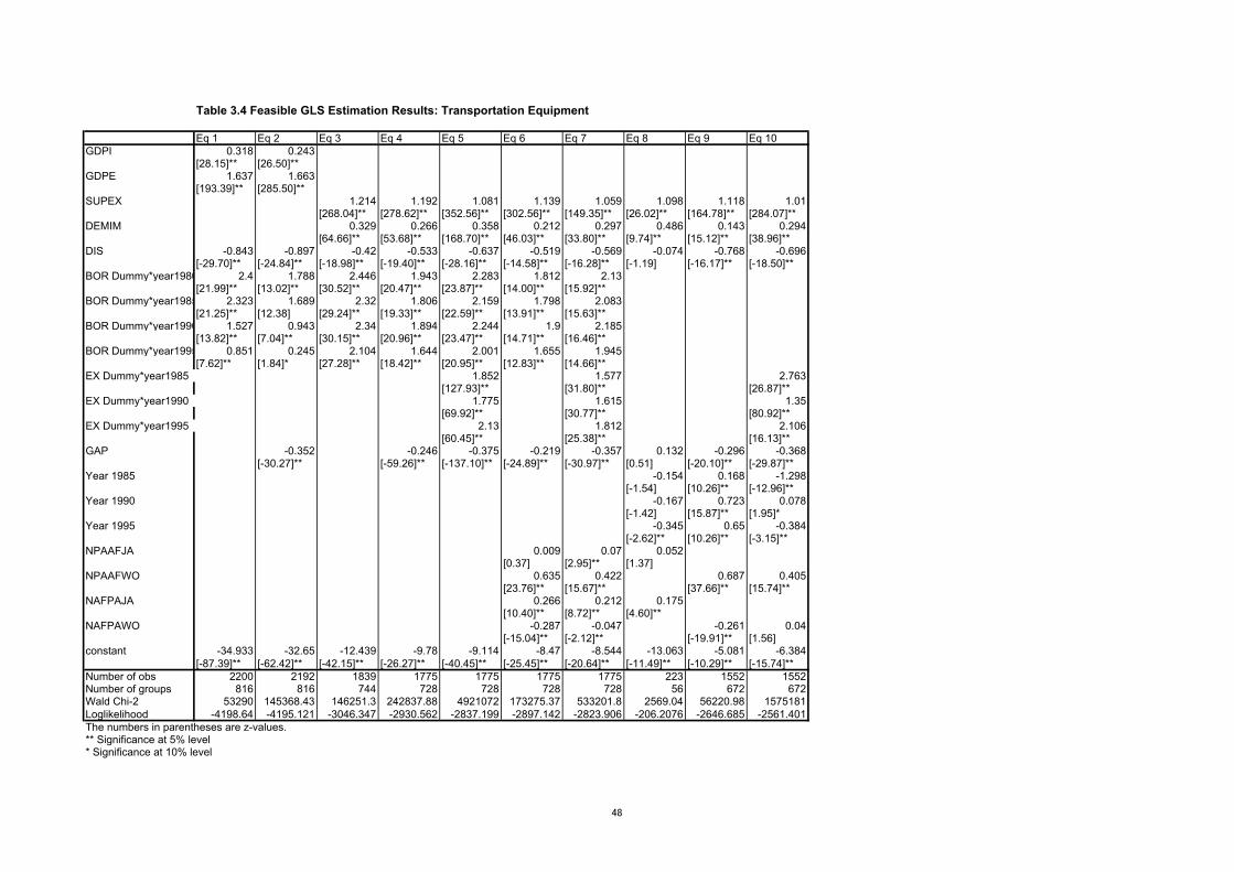
Table 3.4 Feasible GLS Estimation Results: Transportation Equipment

Eq 1 Eq 2 Eq 3 Eq 4 Eq 5 Eq 6 Eq 7 Eq 8 Eq 9 Eq 10GDPI 0.318 0.243

[28.15]** [26.50]**GDPE 1.637 1.663

[193.39]** [285.50]**SUPEX 1.214 1.192 1.081 1.139 1.059 1.098 1.118 1.01

[268.04]** [278.62]** [352.56]** [302.56]** [149.35]** [26.02]** [164.78]** [284.07]**DEMIM 0.329 0.266 0.358 0.212 0.297 0.486 0.143 0.294

[64.66]** [53.68]** [168.70]** [46.03]** [33.80]** [9.74]** [15.12]** [38.96]**DIS -0.843 -0.897 -0.42 -0.533 -0.637 -0.519 -0.569 -0.074 -0.768 -0.696

[-29.70]** [-24.84]** [-18.98]** [-19.40]** [-28.16]** [-14.58]** [-16.28]** [-1.19] [-16.17]** [-18.50]**BOR Dummy*year1980 2.4 1.788 2.446 1.943 2.283 1.812 2.13

[21.99]** [13.02]** [30.52]** [20.47]** [23.87]** [14.00]** [15.92]**BOR Dummy*year1985 2.323 1.689 2.32 1.806 2.159 1.798 2.083

[21.25]** [12.38] [29.24]** [19.33]** [22.59]** [13.91]** [15.63]**BOR Dummy*year1990 1.527 0.943 2.34 1.894 2.244 1.9 2.185

[13.82]** [7.04]** [30.15]** [20.96]** [23.47]** [14.71]** [16.46]**BOR Dummy*year1995 0.851 0.245 2.104 1.644 2.001 1.655 1.945

[7.62]** [1.84]* [27.28]** [18.42]** [20.95]** [12.83]** [14.66]**EX Dummy*year1985 1.852 1.577 2.763

[127.93]** [31.80]** [26.87]**EX Dummy*year1990 1.775 1.615 1.35

[69.92]** [30.77]** [80.92]**EX Dummy*year1995 2.13 1.812 2.106

[60.45]** [25.38]** [16.13]**GAP -0.352 -0.246 -0.375 -0.219 -0.357 0.132 -0.296 -0.368

[-30.27]** [-59.26]** [-137.10]** [-24.89]** [-30.97]** [0.51] [-20.10]** [-29.87]**Year 1985 -0.154 0.168 -1.298

[-1.54] [10.26]** [-12.96]**Year 1990 -0.167 0.723 0.078

[-1.42] [15.87]** [1.95]*Year 1995 -0.345 0.65 -0.384

[-2.62]** [10.26]** [-3.15]**NPAAFJA 0.009 0.07 0.052

[0.37] [2.95]** [1.37]NPAAFWO 0.635 0.422 0.687 0.405

[23.76]** [15.67]** [37.66]** [15.74]**NAFPAJA 0.266 0.212 0.175

[10.40]** [8.72]** [4.60]**NAFPAWO -0.287 -0.047 -0.261 0.04

[-15.04]** [-2.12]** [-19.91]** [1.56]constant -34.933 -32.65 -12.439 -9.78 -9.114 -8.47 -8.544 -13.063 -5.081 -6.384

[-87.39]** [-62.42]** [-42.15]** [-26.27]** [-40.45]** [-25.45]** [-20.64]** [-11.49]** [-10.29]** [-15.74]**Number of obs 2200 2192 1839 1775 1775 1775 1775 223 1552 1552Number of groups 816 816 744 728 728 728 728 56 672 672Wald Chi-2 53290 145368.43 146251.3 242837.88 4921072 173275.37 533201.8 2569.04 56220.98 1575181Loglikelihood -4198.64 -4195.121 -3046.347 -2930.562 -2837.199 -2897.142 -2823.906 -206.2076 -2646.685 -2561.401The numbers in parentheses are z-values.** Significance at 5% level* Significance at 10% level

48