WHY YES, THAT IS HOT GLUE 1

Why Yes, That is Hot Glue:A Simulation Based Approach to Roboboat 2016

Samuel Seifert, Patrick Meyer, James Wittig,Vinayak Ruia, Daniel Findeis

Georgia Institute of Technology

Abstract—This paper describes the development of Burnadette,a fully autonomous surface vehicle for use in the AUVSIRoboboat competition developed by the Georgia Tech ADEPTLab. The vehicle uses a previously manufactured platform toallow for added emphasis on software capabilities. A tightlycoupled simulation environment was developed in parallel to thehardware solutions. This allowed for the development, testing,and integration of various autonomous behavior algorithms foruse in the competition. The simulation environment developedalso includes hardware in the loop capabilities for use in debug-ging and testing. The added simulation capability has allowed forrapid iterations of these behaviors while lessening the need fortime consuming full system tests. We have high hopes that thisprocess will lead to success at this year’s Roboboat competition.

I. INTRODUCTION

Roboboat is held over seven days. For the first five days,participating teams vie for several 30 minute time slots fortesting on the competition course. Over the course of thesedays, teams can expect to get roughly 10 hours of time totest. This is simply not enough time to develop, debug, andtune entire software stack for all of the tasks outlined inthe competition. To adequately prepare for the competition,teams must to supplement this time either by: using data andknowledge from past competitions, testing before the compe-tition at a mock competition site, and testing in simulation.Due to lack of foresight, recorded sensor data from previousRoboboat competitions was not available. Additionally, thenearest suitable testing site to Georgia Tech is a 40 minutedrive away. Collecting real world data at this site requires asignificant time investment, and it would be impossible to testat this site on a day to day basis. Due to these challenges, theteam has decided to augment our testing capabilities throughthe development of a comprehensive simulation environment,called the ADEPT Autonomous Vehicle Simulator (AAVS).Using this environment, different autonomy and control al-gorithms can be designed, implemented, and tested withoutneeding to be at the lake. This allows lake time to be used moreefficiently, verifying and tuning behaviors instead of creatingand debugging them.

The simulation environment has proved incredibly usefulin non-software aspects of the design process too. Ambigu-ous hardware questions, like what LIDAR should be used?and where should the hydrophones be mounted?, can beanswered through virtual experimentation. By running theentire Roboboat competition in AAVS using different sensor

configurations, the performance of each configuration canbe compared using the scoring guidelines outlined by theRoboboat rules as an objective function. This technique en-sures we get the most out of the sensors we have, and can beused to determine which sensors will actually help improveperformance of competition tasks before purchases are made.

The remainder of this paper will outline the developmentof the hardware and software used to compete in this year’sRoboboat competition. This begins with a discussion of ouroverarching design philosophy in II. Design Strategy. Next,the implementation of this strategy in the development ofAAVS and the vehicle hardware used is outlined in III. VehicleDesign. Finally, preliminary results available at this time arepresented in IV. Experimental Results.

II. DESIGN STRATEGY

Roboboat is ultimately an autonomous vehicles competition.Though the vehicle design can improve performance, the mostimportant factors in having a successful system are the au-tonomous behaviors. With this in mind, the Georgia Tech teamadopted a software first approach to the design process. Thisis similar to a common view in the UAV community, wherethe vehicle itself is merely a truck to get the payload where itneeds to be. In this case, the behavioral algorithms themselvescould be considered the payload. The truck necessary couldbe any maneuverable floating platform, provided it supportsthe correct sensors. To minimize the design work necessary toget an adequate platform, a previously designed vehicle wasused. This platform was the vehicle used by the 2014 GeorgiaTech team.

To further reduce workload, the software stack used forsimulation was designed to control the actual competition ve-hicle (as opposed to being two separately developed entities).The simulation and the actual vehicle software are the samestack, which has greatly accelerated the development process.The simulation environment is a great tool because real worldsuccess implies simulation success: i.e. the ideas that fail insimulation can be abandoned because they won’t work inreal life. However only testing in simulation is inadequatebecause simulation success does no imply real world success.To compensate for this phenomena, the team has worked hardto constantly validate the simulation with real world tests.

It is important to understand these two points that highlightdifferent strengths of a simulation based design approach.Though significant effort has been expended to accurately

WHY YES, THAT IS HOT GLUE 2

model the on-board sensors and dynamics of the vehicle,the simulator generally overestimates system performance.As such, ideas that have been implemented in the simulatorwithout success are unlikely to perform any better in the realworld, where additional noise and non-optimal conditions areconstantly present. Similarly, ideas that work in the real worldwill almost certainly work in simulation where conditions areideal.

III. VEHICLE DESIGN

As the design philosophy described above is very muchsoftware first, this section will largely discuss the developmentand capabilities of AAVS. This includes a broad overviewof AAVS itself and it’s capabilities, the dynamic model andstate estimator used, and a sampling of the implementedautonomous behavior algorithms. Following this will be a briefdescription of the hardware systems used.

A. Simulation Environment

AAVS was built from scratch in C#. Using data extractedfrom Google Maps, knowledge retained from previous yearscompetitions, and the preliminary rules for this year, the 2016Roboboat course has been laid out in the simulation environ-ment as shown in Fig. 1 inside AAVS. Using this environmentto develop algorithms and the overarching software stack hasproved invaluable.

Figure 1: The 2016 Roboboat course in simulation.

Initial analysis showed four sensor subsystems were re-quired to gather adequate information from the environmentto complete the Roboboat tasks:

• GPS & IMU to determine vehicle state.• LIDAR system to detect physical obstacles.• Camera system to recognize color & pattern.• Sonar system to locate the pinger.Models for sensors in each of these four categories have

been developed for use in AAVS. These models have beenvalidated against real world experiments to show they cangenerate representative data. In the current version of the

simulator, GPS, IMU, and LIDAR data can be realisticallygenerated (as shown in Figure 2), while camera and sonardata remain unrealistic. Because of this, most of the autonomyalgorithms developed rely primarily on GPS, IMU and LIDARdata, and only use the cameras and sonar systems when specif-ically needed. However, this has proven to be sufficient in realworld tests. A suitable dynamic model has been implementedto estimate the vehicle’s response to command inputs as wellas an Extended Kalman Filter and will be described in furtherdetail in the following section.

B. System Dynamics

For the simulation environment to generate representativetraining runs, a reasonable model for how the vehicle movesthrough the water is needed. While there has been work onthree-dimensional dynamic models for small marine vehicles[1], a two-dimensional model, considering yaw, surge, andsway while ignoring pitch, roll, and heave has been imple-mented. Ignoring pitch, roll, and heave is common practicefor small surface vehicles [2] in low sea states where affectslike broaching can be ignored. For propulsion, the vehicleis equipped with four SeaBotix BTD150 thrusters in a skidsteering configuration. Two thrusters are along the centerlineof the vehicle, and they can be used to accelerate/deceleratein the longitudinal direction. The remaining two thrusters areon either side of the vehicle, and can be used to acceler-ate/decelerate in the longitudinal direction and apply a torqueto induce rotation. As such, the dynamic model consists ofthese states:

• θ - angular position (yaw) in world frame• ω - angular velocity in world frame• x - position in world frame• y - position in world frame• u - linear velocity (surge) in vehicle frame• v - linear velocity (sway) in vehicle frame

And the following inputs:• ml - force applied by left motor• mc - force applied by center motors• mr - force applied by right motorSeaBotix provides a thrust to voltage curve for these mo-

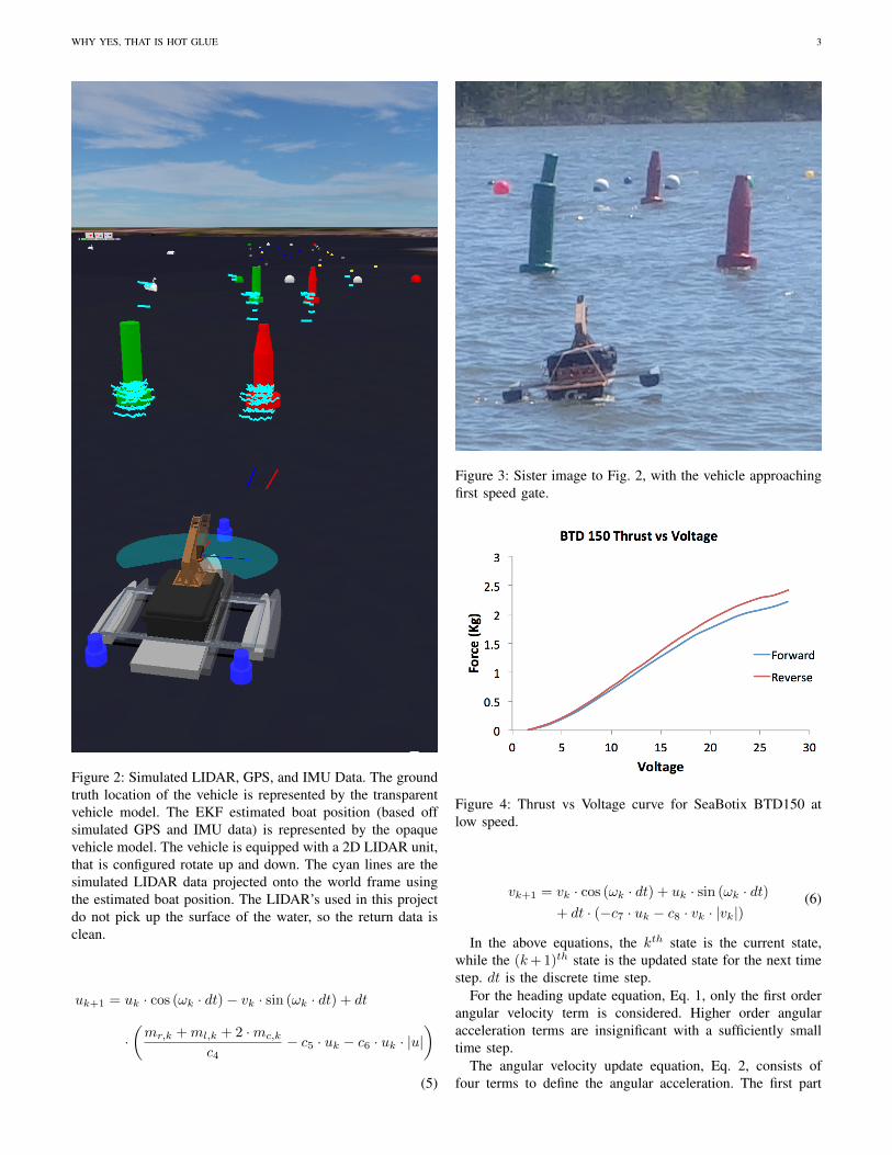
tors at low speeds as shown in Fig. 4. This thrust-voltagerelationship was used to build a transfer function to estimatethe applied forces for given throttle inputs. The state updateequations for the dynamic model are dictated by the followingequations:

(1)θk+1 = θk + ωt · dt

(2)ωk+1 = ωk + dt ·

(mr,k −ml,k

c1− c2 · wk − c3 · wk

· |wk|+c9 ·(u2k + v2k

)· sin (atan2 (vk, uk))

)(3)xk+1 = xk + dt · (uk · cos (θ) + vk · sin (θ))

(4)yk+1 = yk + dt · (vk · cos (θ) + uk · sin (θ))

WHY YES, THAT IS HOT GLUE 3

Figure 2: Simulated LIDAR, GPS, and IMU Data. The groundtruth location of the vehicle is represented by the transparentvehicle model. The EKF estimated boat position (based offsimulated GPS and IMU data) is represented by the opaquevehicle model. The vehicle is equipped with a 2D LIDAR unit,that is configured rotate up and down. The cyan lines are thesimulated LIDAR data projected onto the world frame usingthe estimated boat position. The LIDAR’s used in this projectdo not pick up the surface of the water, so the return data isclean.

uk+1 = uk · cos (ωk · dt)− vk · sin (ωk · dt) + dt

·(mr,k +ml,k + 2 ·mc,k

c4− c5 · uk − c6 · uk · |u|

)(5)

Figure 3: Sister image to Fig. 2, with the vehicle approachingfirst speed gate.

Figure 4: Thrust vs Voltage curve for SeaBotix BTD150 atlow speed.

(6)vk+1 = vk · cos (ωk · dt) + uk · sin (ωk · dt)+ dt · (−c7 · uk − c8 · vk · |vk|)

In the above equations, the kth state is the current state,while the (k+1)th state is the updated state for the next timestep. dt is the discrete time step.

For the heading update equation, Eq. 1, only the first orderangular velocity term is considered. Higher order angularacceleration terms are insignificant with a sufficiently smalltime step.

The angular velocity update equation, Eq. 2, consists offour terms to define the angular acceleration. The first part

WHY YES, THAT IS HOT GLUE 4

term consists of the input torque mr − ml divided by thevehicle rotational inertia c1. The length of the moment armfor these torques is captured in the rotational inertia term.The next two terms approximate the first (c2) and second (c3)order angular damping of the vehicle. The final term representsa straightening phenomena, designed to capture the vehiclesnatural tendency to glide straight through the water.

The global position update equations, Eq. 3 and 4, onlycontain the first order velocity terms without higher orderacceleration terms. This is done with the same assumptionof a sufficiently small time step. The sin(θ) and cos(θ) termstransform the velocity terms u and v from vehicle frame toworld frame.

The surge update equation, Eq. 5, involves transforming thevelocity in vehicle frame as the vehicle frame rotates. Thenext term is the linear force divided by the system inertia (c4).The last two terms are first (c5) and second (c6) order dragapproximations. The sway update equation, Eq. 6, is identicalto surge with the exception of the removed force/inertia term.

For this model to be useful, values for the nine constants thatappear in the state equations need to be assigned, estimated,or measured. Some of these constants (like mass) can bemeasured directly, while other constants need to be estimated.Initially, online parameter estimated with a recursive leastsquares (RLS) estimator was attempted. However, the onlineversion proved unstable and an offline parameter estimator wasused to determine these coefficients. For the offline parameterestimator, an hours worth of GPS and IMU data (of thevehicle driving on the lake in a predetermined pattern) wasrecorded. GPS data consists of the vehicle global positionat a 4 Hz update rate, and the IMU data consists of 3DMagnetometer, Gyroscope, and Accelerometer data at 100Hz. 95% of the GPS data was withheld and used to train& determine dynamic model coefficients. A gradient descentoptimizer was configured to minimize the mean-square-error(MSE) of the withheld GPS data with the predicted modellocation. In other words, we:

1) Split data into 5 second time intervals.2) Withheld all the GPS data (except the very first data

point in each time intervals) from each interval.3) Seed dynamic model with an estimate of what the boat

is doing at that very first point for each interval.4) Evolve the dynamic model 5 seconds into the future,

using only the recorded input (motor voltages) for thatinterval.

5) Compare the withheld GPS data with predicted pathfrom dynamic model.

6) Perform gradient descent on model parameters to mini-mize the MSE between withheld and prediction data.

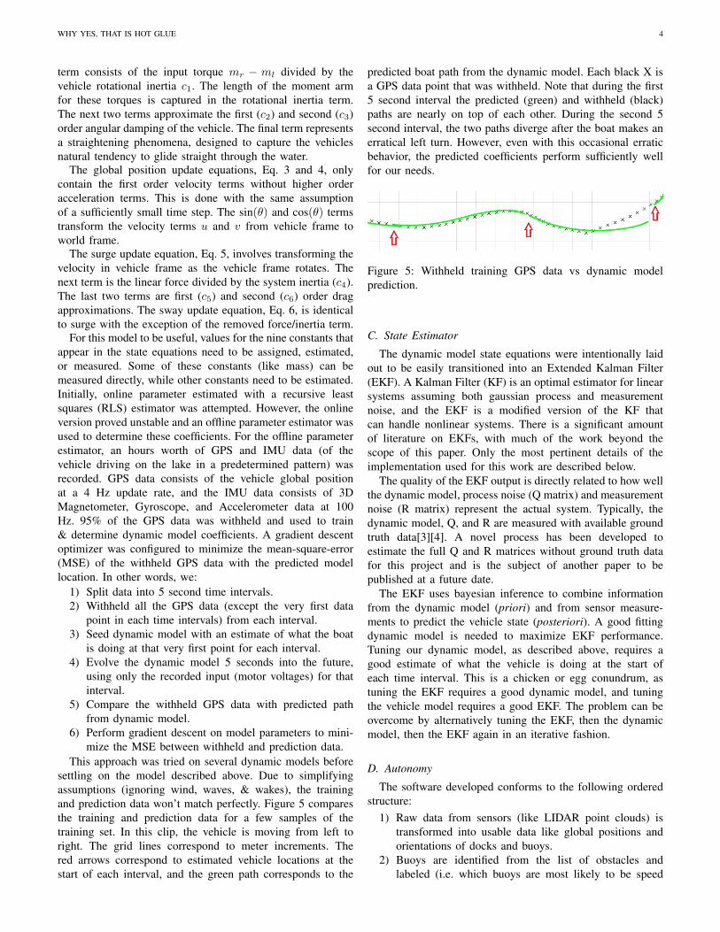
This approach was tried on several dynamic models beforesettling on the model described above. Due to simplifyingassumptions (ignoring wind, waves, & wakes), the trainingand prediction data won’t match perfectly. Figure 5 comparesthe training and prediction data for a few samples of thetraining set. In this clip, the vehicle is moving from left toright. The grid lines correspond to meter increments. Thered arrows correspond to estimated vehicle locations at thestart of each interval, and the green path corresponds to the

predicted boat path from the dynamic model. Each black X isa GPS data point that was withheld. Note that during the first5 second interval the predicted (green) and withheld (black)paths are nearly on top of each other. During the second 5second interval, the two paths diverge after the boat makes anerratical left turn. However, even with this occasional erraticbehavior, the predicted coefficients perform sufficiently wellfor our needs.

Figure 5: Withheld training GPS data vs dynamic modelprediction.

C. State Estimator

The dynamic model state equations were intentionally laidout to be easily transitioned into an Extended Kalman Filter(EKF). A Kalman Filter (KF) is an optimal estimator for linearsystems assuming both gaussian process and measurementnoise, and the EKF is a modified version of the KF thatcan handle nonlinear systems. There is a significant amountof literature on EKFs, with much of the work beyond thescope of this paper. Only the most pertinent details of theimplementation used for this work are described below.

The quality of the EKF output is directly related to how wellthe dynamic model, process noise (Q matrix) and measurementnoise (R matrix) represent the actual system. Typically, thedynamic model, Q, and R are measured with available groundtruth data[3][4]. A novel process has been developed toestimate the full Q and R matrices without ground truth datafor this project and is the subject of another paper to bepublished at a future date.

The EKF uses bayesian inference to combine informationfrom the dynamic model (priori) and from sensor measure-ments to predict the vehicle state (posteriori). A good fittingdynamic model is needed to maximize EKF performance.Tuning our dynamic model, as described above, requires agood estimate of what the vehicle is doing at the start ofeach time interval. This is a chicken or egg conundrum, astuning the EKF requires a good dynamic model, and tuningthe vehicle model requires a good EKF. The problem can beovercome by alternatively tuning the EKF, then the dynamicmodel, then the EKF again in an iterative fashion.

D. Autonomy

The software developed conforms to the following orderedstructure:

1) Raw data from sensors (like LIDAR point clouds) istransformed into usable data like global positions andorientations of docks and buoys.

2) Buoys are identified from the list of obstacles andlabeled (i.e. which buoys are most likely to be speed

WHY YES, THAT IS HOT GLUE 5

gates, or obstacle entrance & exit gates, or the buoywith the active pinger).

3) Gate, dock, and pinger locations are transformed into adestination based on the planner that takes into accountthe current and completed tasks for the overall mission.

4) The arbiter takes the destination, obstacles list, and othersensor data and determines how to get there withouthitting anything.

5) The controller transforms the arbiter command (directionand heading) into motor voltages, keeping the vehicle oncourse & stable.

Some specialized algorithms combine two more more ofthese steps, but for most configurations the above list repre-sents how data flows through the software. There are manydifferent moving parts, and many of these steps have beenimplemented in more than one way. It would be impossibleto cover the entire software in the space of this paper, so arepresentative sample is presented here.

1) Acoustic Pinger Localization: The vehicle is equippedwith three hydrophones. The hydrophone layout is shownin Fig. 2, with the blue cylinders representing hydrophonelocations. Each hydrophone returns a raw audio signal which,when filtered and amplified, can be turned into a series oftimestamps that correspond to when the hydrophone detecteda ping. There are several ways to use these timestamps toestimate pinger location. The best performing algorithm thathas been implemented is a RANSAC locater[5].

If two hydrophones recorded the same event at the sametime, the pinger must be equidistant from both hydrophones.This is illustrated in Fig. 6, with the red circles representinghydrophones and the blue line representing the continuous setof possible pinger locations.

Figure 6: Continuous set of pinger locations (blue) given thatsome event was recorded by two hydrophones (red) at thesame time.

This blue line is also called an contour line, signifying thatfor any point on the line, the time difference between whenthe sound reaches both hydrophones is constant. A nonzero

time difference would correspond to a different contour line,as shown in Fig. 7. The increment in time difference valuesbetween adjacent contour lines in this graph is constant. Thenonuniform angular resolution illustrated in Fig. 7 highlightsthe fact that estimated pinger position accuracy is sensitive tothe orientation of the hydrophone pair relative to the pinger.

Figure 7: Contour lines for a two hydrophone sonar array.

With multiple hydrophone pairs, it is possible to combinethe information from the contour lines to triangulate theposition of the pinger. Alternatively, a single hydrophone paircould estimate the position of a stationary pinger by collectingseveral data from several different locations. For either of thesemethods, an accurate estimate of the vehicles state, and therelative orientation of the hydrophones to the vehicles frame isnecessary. In practice, it helps to both have more than two hy-drophones, and move the vehicle while data is being recorded.This is illustrated using the simulation environment in Fig. 8and Fig. 9. Finding an optimal configuration for hydrophoneplacement analytically, especially considering the couplingwith the EKF and autonomous behavior, is impossible. Usingthe simulation environment, however, a local optimal solutioncan be found.

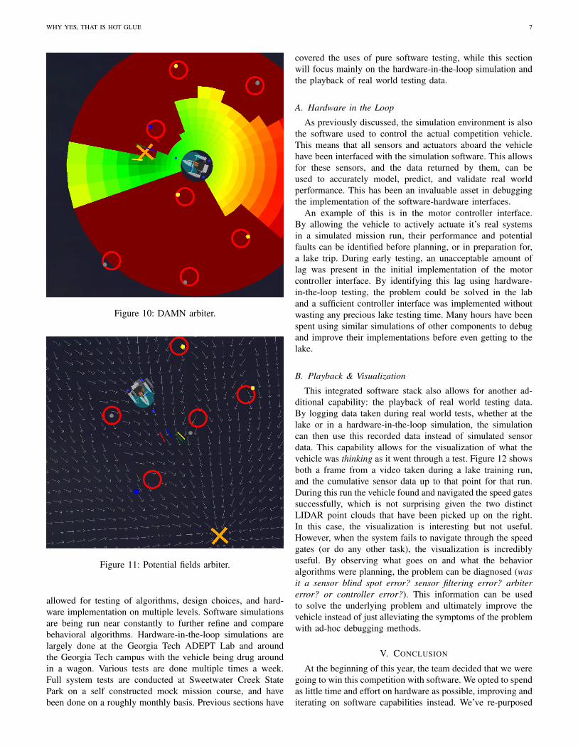
2) DAMN Arbiter: Distributed architecture for mobile nav-igation or (DAMN) is a reactive architecture that arbitratesthrough voting [6]. The local region around the vehicle isbroken up into smaller sub regions, and each behavior (inthis case both go to waypoint and avoid obstacles) votes onhow willing that behavior is to travel to that region. Theseregions are illustrated in Fig. 10; where color correspondsto vote total. Green indicates a high vote, or a willingnessfor the vehicle to head to that region. Red indicates a lowvote or an unwillingness to head to that region. Differentbehaviors have a different voting weight. The avoid obstaclesbehavior has the strongest vote, which is why the regions nearperceived obstacles (indicated by red circles) are dark red. Toavoid situations where the goal point is directly behind anobstacle, the avoid obstacle behavior also negatively votes forany areas that are obstructed by known obstacles. The orange

WHY YES, THAT IS HOT GLUE 6

Figure 8: RANSAC for single ping on a three hydrophonevehicle. The system misses (green cross) the pinger (red buoy)because the contour lines are almost all parallel.

cross indicates the current destination, and, as expected, issurrounded by the greenest regions. The arbiter commands thevehicle to head toward the region with the highest vote total,with a speed that’s proportional to how far the region is fromthe vehicle.

3) Potential Fields Arbiter: Another arbiter that has beenimplemented and tested is arbitration through a potentialfield abstraction. Each behavior now acts as either a source,such as avoiding obstacles, or a sink, such as a waypointdestination. A weighted average of the resulting fields is taken,again with avoid obstacles having the dominant weight, andheading and velocity is returned. This return is produced via asimple gradient descent through the potential space. Figure 11illustrates the average vector returned by the arbiter at variouslocations, indicated by the white arrows. The orange crossdenotes the waypoint sink and red circles denote perceivedobstacles acting as sources in the potential field.

The simulation environment has been used to compareperformance of these two (and other) arbitration techniques.Visualizations within the software provide insight to not onlywhich algorithms perform best, but also why they performbest.

E. Hardware Description

An existing platform that had been used in past Roboboatcompetitions was repurposed for this year’s competition. Thevehicle frame itself is a trimaran design. Propulsion is providedby four Seabotix electric motors arrayed in a skid steering

Figure 9: RANSAC for three pings on a three hydrophonevehicle. The system returns (green cross) a much betterestimate for pinger (red buoy) location because the contourlines are not all parallel.

configuration. Onboard computing is handled by an Intel NUCwith a Core i7 processor running Windows 10. The computeris interfaced with the DC motor controllers using an ArduinoMega microprocessor and packetized serial communication. AHokuyo UTM-30LX planar LIDAR actuated by a DynamixelAX-12A servo is used for 3D obstacle detection and clas-sification. A Microstrain 3DM-GX3-45 INS is used for anonboard GPS and IMU system. All electronic componentsare housed in a waterproof Pelican Storm iM2400 cases. Thecase has been outfitted with a modular component rack andcustom power rail system. The motors and other electronicsare decoupled on separate circuits, with a 5 cell LiPo batteryused for motor power, and a 4 cell LiPo battery used for thecomputer and sensor systems.

IV. EXPERIMENTAL RESULTS

Much of this paper has discussed the value of the AAVSenvironment. One of the key features of this environmentis the integrated stack used for simulation, hardware-in-the-loop testing, and control of the competition vehicle. This has

WHY YES, THAT IS HOT GLUE 7

Figure 10: DAMN arbiter.

Figure 11: Potential fields arbiter.

allowed for testing of algorithms, design choices, and hard-ware implementation on multiple levels. Software simulationsare being run near constantly to further refine and comparebehavioral algorithms. Hardware-in-the-loop simulations arelargely done at the Georgia Tech ADEPT Lab and aroundthe Georgia Tech campus with the vehicle being drug aroundin a wagon. Various tests are done multiple times a week.Full system tests are conducted at Sweetwater Creek StatePark on a self constructed mock mission course, and havebeen done on a roughly monthly basis. Previous sections have

covered the uses of pure software testing, while this sectionwill focus mainly on the hardware-in-the-loop simulation andthe playback of real world testing data.

A. Hardware in the Loop

As previously discussed, the simulation environment is alsothe software used to control the actual competition vehicle.This means that all sensors and actuators aboard the vehiclehave been interfaced with the simulation software. This allowsfor these sensors, and the data returned by them, can beused to accurately model, predict, and validate real worldperformance. This has been an invaluable asset in debuggingthe implementation of the software-hardware interfaces.

An example of this is in the motor controller interface.By allowing the vehicle to actively actuate it’s real systemsin a simulated mission run, their performance and potentialfaults can be identified before planning, or in preparation for,a lake trip. During early testing, an unacceptable amount oflag was present in the initial implementation of the motorcontroller interface. By identifying this lag using hardware-in-the-loop testing, the problem could be solved in the laband a sufficient controller interface was implemented withoutwasting any precious lake testing time. Many hours have beenspent using similar simulations of other components to debugand improve their implementations before even getting to thelake.

B. Playback & Visualization

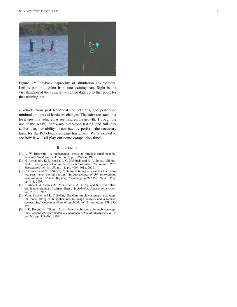
This integrated software stack also allows for another ad-ditional capability: the playback of real world testing data.By logging data taken during real world tests, whether at thelake or in a hardware-in-the-loop simulation, the simulationcan then use this recorded data instead of simulated sensordata. This capability allows for the visualization of what thevehicle was thinking as it went through a test. Figure 12 showsboth a frame from a video taken during a lake training run,and the cumulative sensor data up to that point for that run.During this run the vehicle found and navigated the speed gatessuccessfully, which is not surprising given the two distinctLIDAR point clouds that have been picked up on the right.In this case, the visualization is interesting but not useful.However, when the system fails to navigate through the speedgates (or do any other task), the visualization is incrediblyuseful. By observing what goes on and what the behavioralgorithms were planning, the problem can be diagnosed (wasit a sensor blind spot error? sensor filtering error? arbitererror? or controller error?). This information can be usedto solve the underlying problem and ultimately improve thevehicle instead of just alleviating the symptoms of the problemwith ad-hoc debugging methods.

V. CONCLUSION

At the beginning of this year, the team decided that we weregoing to win this competition with software. We opted to spendas little time and effort on hardware as possible, improving anditerating on software capabilities instead. We’ve re-purposed

WHY YES, THAT IS HOT GLUE 8

Figure 12: Playback capability of simulation environment.Left is par of a video from one training run. Right is thevisualization of the cumulative sensor data up to that point forthat training run.

a vehicle from past Roboboat competitions, and performedminimal amounts of hardware changes. The software stack thatleverages this vehicle has seen incredible growth. Through theuse of the AAVS, hardware-in-the-loop testing, and full testsat the lake, our ability to consistently perform the necessarytasks for the Roboboat challenge has grown. We’re excited tosee how it will all play out come competition time!.

REFERENCES

[1] A. W. Browning, “A mathematical model to simulate small boat be-haviour,” Simulation, vol. 56, no. 5, pp. 329–336, 1991.

[2] H. Ashrafiuon, K. R. Muske, L. C. McNinch, and R. A. Soltan, “Sliding-mode tracking control of surface vessels,” Industrial Electronics, IEEETransactions on, vol. 55, no. 11, pp. 4004–4012, 2008.

[3] C. Goodall and N. El-Sheimy, “Intelligent tuning of a kalman filter usinglow-cost mems inertial sensors,” in Proceedings of 5th InternationalSymposium on Mobile Mapping Technology (MMT’07), Padua, Italy,pp. 1–8, 2007.

[4] P. Abbeel, A. Coates, M. Montemerlo, A. Y. Ng, and S. Thrun, “Dis-criminative training of kalman filters.,” in Robotics: Science and systems,vol. 2, p. 1, 2005.

[5] M. A. Fischler and R. C. Bolles, “Random sample consensus: a paradigmfor model fitting with applications to image analysis and automatedcartography,” Communications of the ACM, vol. 24, no. 6, pp. 381–395,1981.

[6] J. K. Rosenblatt, “Damn: A distributed architecture for mobile naviga-tion,” Journal of Experimental & Theoretical Artificial Intelligence, vol. 9,no. 2-3, pp. 339–360, 1997.