Wi-Fi Denial of Service Attack on Wired Analog RF … · Wi-Fi Denial of Service Attack on Wired Analog RF ... and a software defined radio called a Universal Software Radio Peripheral

This work was sponsored by the Department of Defense Research and Engineering under

contract number XXXXXXXXXXXXXX. Opinions, interpretations, conclusions and

recommendations are those of the authors and are not necessarily endorsed by the United States

Government.

Wi-Fi Denial of Service Attack on Wired Analog RF

Channel Emulator

A Major Qualifying Project Report

Submitted to the Faculty

of the

WORCESTER POLYTECHNIC INSTITUTE

in partial fulfillment of the requirements for the

Degree of Bachelor of Science

in

Electrical and Computer Engineering

by

__________________________

Sheila Werth

__________________________

Jeffrey Peter Wyman

Project Number: MQP-AW1-12LL

Date: 10/17/2012

Sponsoring Organization:

MIT Lincoln Laboratory

Project Advisors:

____________________________

Professor Alexander M. Wyglinski

Abstract

In this report we designed and implemented a wireless channel emulator to examine various

wireless denial of service attacks. The scenarios emulated in this project involve three different

changing configurations of radios and three different denial of service waveforms. The testbed

was functional and met the original specifications. Of the three denial of service waveforms,

binary phase shift keying was found to be the most effective at decreasing total network

throughput while the chirp signal began to effect network throughput at a greater distance from

the network then any of the other waveforms.

Statement of Authorship

Acknowledgements

We would like to extend our gratitude to the many people that helped to support this project

effort:

MIT Lincoln Laboratory, Group 63

Kenneth Hetling, PhD

James Vian, PhD

William O’Connell

Frank Bieberly

Robert Elliot

Jonathan Chisum, PhD

Todd Brick

Catherine Holland

Carl Fossa, PhD

Worcester Polytechnic Institute

Prof. Alexander Wyglinski

Prof. Ted Clancy

Executive Summary

Emergency response and communications during a major disaster have become increasingly

important over the past decade. In cases such as the L.A. earthquake in 1994, the earthquake and

tsunami in Indonesia, or Hurricane Katrina, the communications infrastructure was overwhelmed

[1] and prevented local law enforcement and emergency personnel from coordinating rescues

and conveying vital information [2]. The damage to the network is not always physical; often

there is major disruption from network congestion [3]. Many networks are not designed to

handle high volumes and the powerful human need to communicate during a disaster can

overwhelm even the most sophisticated networks [4].

The FCC sponsors emergency communication systems such as the Nationwide Wireless Priority

Service (WPS) that allows emergency telephone calls to avoid network congestion, and the

Government Emergency Telecommunications Service (GETS). However, the effectiveness of

these systems has been questioned [6], and the FCC has recently allocated portions of its Public

Safety spectrum for shared commercial use [7]. If these resources become unavailable during a

crisis, emergency responders may prefer to use high-speed wireless internet services [5] which

are equally subject to network congestion. A standard resolution of how emergency responders

and local law enforcement may clear the channel for high-priority use has not yet been proposed.

There is currently not enough exclusive spectrum for emergency responders to reliably

communicate during a crisis. Additionally, recent laws regulating public safety spectrum for

commercial use suggest it may be especially vulnerable to congestion. For these reasons it is

critical for emergency personnel to have the capacity to silence interfering emitters during

disasters so that appropriate response measures may be coordinated. Experimenting with and

validating denial of service techniques over open air-waves could potentially disrupt user

services and violate FCC regulations.

A controllable test platform is needed to investigate the reallocation of spectrum resources in a

contested communications environment. The team designed, built, and calibrated a testbed for

this purpose. Several key specifications were determined early on to ensure that the testbed met

current and future testing needs.

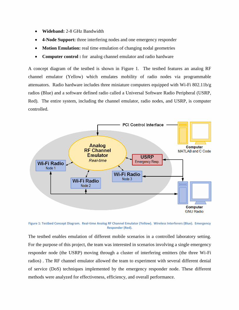
Wideband: 2-8 GHz Bandwidth

4-Node Support: three interfering nodes and one emergency responder

Motion Emulation: real time emulation of changing nodal geometries

Computer control : for analog channel emulator and radio hardware

A concept diagram of the testbed is shown in Figure 1. The testbed features an analog RF

channel emulator (Yellow) which emulates mobility of radio nodes via programmable

attenuators. Radio hardware includes three miniature computers equipped with Wi-Fi 802.11b/g

radios (Blue) and a software defined radio called a Universal Software Radio Peripheral (USRP,

Red). The entire system, including the channel emulator, radio nodes, and USRP, is computer

controlled.

Figure 1: Testbed Concept Diagram. Real-time Analog RF Channel Emulator (Yellow). Wireless Interferers (Blue). Emergency Responder (Red).

The testbed enables emulation of different mobile scenarios in a controlled laboratory setting.

For the purpose of this project, the team was interested in scenarios involving a single emergency

responder node (the USRP) moving through a cluster of interfering emitters (the three Wi-Fi

radios) . The RF channel emulator allowed the team to experiment with several different denial

of service (DoS) techniques implemented by the emergency responder node. These different

methods were analyzed for effectiveness, efficiency, and overall performance.

In order to ensure that the testbed met specifications and was representative of a time-varying RF

channel, the team conducted a variety of tests on the parts and the system as a whole. S-

parameters were measured across the band for each part. Switching speed was measured for the

attenuators. When the testbed was assembled, loss was measured throughout the system for each

of the twelve possible routes through the system and calibrated to make sure that variation

between those routes was minimal. A photograph of the assemble system is shown below in

Figure 4.

Figure 4: Assembled Testbed. Wi-Fi Radios & USRP (Left), Real-time Analog RF Channel Emulator (Middle), Computer Based Control (Right). All components are controlled through one central computer (not shown).

To further confirm that the testbed would produce reasonable results, measurements taken on a

stationary two node network, similar to one described in the literature [7], were compared to

measurements taken on the four radio testbed. Comparing the four node team testbed with the

previously described two radio configuration served as a verification and validation of the

procedures and equipment used during the course of this project. Results from this comparison

are shown in Figure 3.

Figure 3: Verification and Validation: Comparison of Throughput vs. SWR between Two Node Testbed (Top) and Four Node Testbed with Channel Emulator (Bottom). Both testbed results are comparable to published research [7].

The graphs shown in Figure 3 plot the throughput in the network for different Signal to

Waveform Ratios. For the purpose of this experiment, the ‘waveform’ is a digital signal,

modulated with binary phase shift keying, meant to interrupt network communications. With a

greater Signal to Waveform Ratio, higher throughput would be expected, as shown in Figure 3.

With nearly identical results for the well known two radio network and on the team-built four

radio testbed, it is reasonable to infer that they produce similar channel conditions.

Once the testbed had been built, tested, and validated, a series of three mobile node scenarios,

along with three different denial of service waveforms, were selected for investigation on the

testbed. Each waveform was implemented on each of the three mobile scenarios. For simplicity,

wireless nodes were made stationary while the emergency responder traversed a straight path at a

constant velocity. The three different denial of service waveforms include digital, pulse, and

sweep. Figure 5 displays the results of one experimental mobile scenario repeated for each denial

of service waveforms; (A) displays total network throughput over time when subject to a

jammer waveform, (B) illustrates the position of each stationary node with the start and stop

location of the emergency responder.

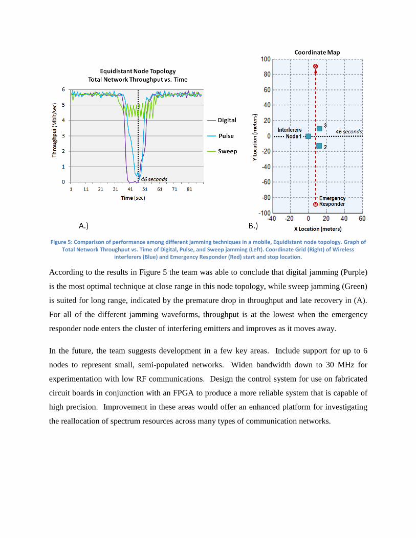
Figure 5: Comparison of performance among different jamming techniques in a mobile, Equidistant node topology. Graph of Total Network Throughput vs. Time of Digital, Pulse, and Sweep jamming (Left). Coordinate Grid (Right) of Wireless

interferers (Blue) and Emergency Responder (Red) start and stop location.

According to the results in Figure 5 the team was able to conclude that digital jamming (Purple)

is the most optimal technique at close range in this node topology, while sweep jamming (Green)

is suited for long range, indicated by the premature drop in throughput and late recovery in (A).

For all of the different jamming waveforms, throughput is at the lowest when the emergency

responder node enters the cluster of interfering emitters and improves as it moves away.

In the future, the team suggests development in a few key areas. Include support for up to 6

nodes to represent small, semi-populated networks. Widen bandwidth down to 30 MHz for

experimentation with low RF communications. Design the control system for use on fabricated

circuit boards in conjunction with an FPGA to produce a more reliable system that is capable of

high precision. Improvement in these areas would offer an enhanced platform for investigating

the reallocation of spectrum resources across many types of communication networks.

Table of Contents

ABSTRACT .............................................................................................................................................................. 2

STATEMENT OF AUTHORSHIP ................................................................................................................................ 3

ACKNOWLEDGEMENTS .......................................................................................................................................... 4

EXECUTIVE SUMMARY ........................................................................................................................................... 5

LIST OF FIGURES ................................................................................................................................................... 12

LIST OF TABLES .................................................................................................................................................... 19

LIST OF ACRONYMS ............................................................................................................................................. 20

1 INTRODUCTION ............................................................................................................................................ 1

1.1 MOTIVATION ....................................................................................................................................................... 1

1.2 PROBLEM STATEMENTS ......................................................................................................................................... 2

1.3 PROPOSED SOLUTION ............................................................................................................................................ 2

1.4 REPORT ORGANIZATION ........................................................................................................................................ 4

2 OVERVIEW OF RF CHANNELS, WIRELESS NETWORKS, AND SECURITY .......................................................... 6

2.1 THE RF CHANNEL ................................................................................................................................................. 6

Important aspects of RF channel .......................................................................................................................... 6 Creating experimental channel conditions ......................................................................................................... 12

2.2 WIRELESS COMMUNICATION & SECURITY ............................................................................................................... 22

Brief Tutorial in Wireless Communications and 802.11b/g ................................................................................ 22 PHY Layer ........................................................................................................................................................... 25 MAC Layer .......................................................................................................................................................... 36 Different types of jamming and attacks ............................................................................................................. 41

3 METHODS ................................................................................................................................................... 46

3.1 TESTBED DESIGN PROCESS .................................................................................................................................... 46

Original Design Ideas and Assessment ............................................................................................................... 47 Final Design ........................................................................................................................................................ 51

3.2 ATTENUATOR CONTROL ....................................................................................................................................... 54

3.3 TESTBED CONSTRUCTION AND PRELIMINARY TESTING ................................................................................................. 56

3.4 PHY LAYER JAMMING .......................................................................................................................................... 59

Validating the Testbed against Previous Experiments ....................................................................................... 60 Mobile PHY Layer Jamming on the RF Channel Emulator .................................................................................. 61

3.5 MAC LAYER JAMMING ........................................................................................................................................ 69

Original Idea: Reactive Beacon Frame Injection ................................................................................................. 69

4 RESULTS ...................................................................................................................................................... 73

4.1 CHANNEL EMULATOR: TESTING AND VALIDATION ..................................................................................................... 73

Assembled RF Analog Channel Testbed .............................................................................................................. 80 Testing and measurements on the assembled system ....................................................................................... 83

4.2 WI-FI MOBILE JAMMING EXPERIMENTS ................................................................................................................... 96

4.2.1 MAC Layer Mobile Jamming .............................................................................................................. 113

5 CONCLUSIONS AND FUTURE WORK .......................................................................................................... 114

6 REFERENCES .............................................................................................................................................. 117

7 APPENDIX ................................................................................................................................................. 121

MATLAB Code: Calculate Programmable Attenuator Values ........................................................................... 124 MATLAB Code: Generate ASCII Characters ....................................................................................................... 126 C Code: Write to NI-PCI Card ............................................................................................................................ 127 Datasheet: Krytar Coupler ................................................................................................................................ 130

List of Figures

Figure 1: Proposed solution, computer controlled RF testbed with real-time channel emulation,

Universal Software Radio Peripheral (USRP) and commercially available Wi-Fi Radios 3

Figure 2: Channel model considering sources of interference [13]. This model includes a scaled

and delayed signal, multipath fading, narrowband noises and broadband noises. ............. 7

Figure 3: Obstacles cause electromagnetic waves to reflect and travel different paths of varying

lengths. The red path, path 1, is the line of site path while the blue path, path 2, is the

result of reflected signal power. Signal power traveling path two travels a greater distance

and thus experiences greater delay. The sum of the power from both paths is a signal that

is distorted due to multipath effects. ................................................................................... 9

Figure 4: (A) Noiseless time domain 60Hz signal. (B) Noiseless 60 Hz frequency domain signal.

(C) 60 Hz time domain signal with AWGN (Blue) and noiseless 60Hz time domain

signal. (D) Noisy 60 Hz signal in the frequency domain, the noise floor is shown in red.

........................................................................................................................................... 11

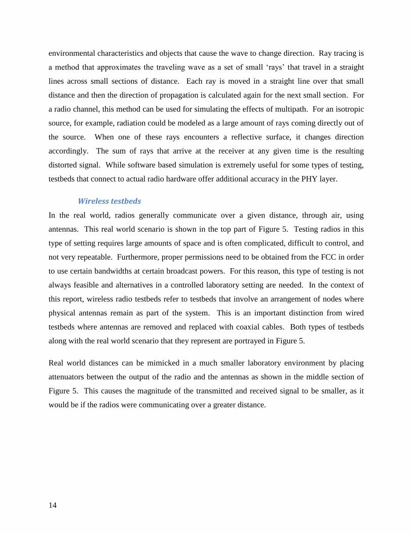
Figure 5: The real world radio communications scenario, shown on top, can be modeled using a

wireless, miniaturized, configuration with attenuators (middle). The concept of a wired

testbed is at the bottom of the image. A wired testbed involves radios that are connected

to each other using coaxial cable and RF components, like the attenuator shown, to model

channel response. .............................................................................................................. 14

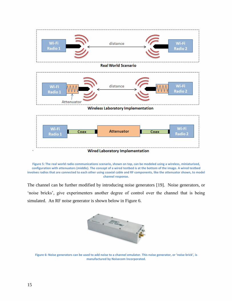
Figure 6: Noise generators can be used to add noise to a channel emulator. This noise generator,

or ‘noise brick’, is manufactured by Noisecom Incorporated. .......................................... 14

Figure 7: The indoor testing facility at Rutgers University [21] is open for use to members of the

research community who write their own code. Each yellow box is one of 400 stationary

radio nodes. ....................................................................................................................... 15

Figure 8: In the EWANT testbed, antennas can be rearranged on metallic table top with holes to

create unique geometries. By switching between antennas, mobility can be emulated. .. 16

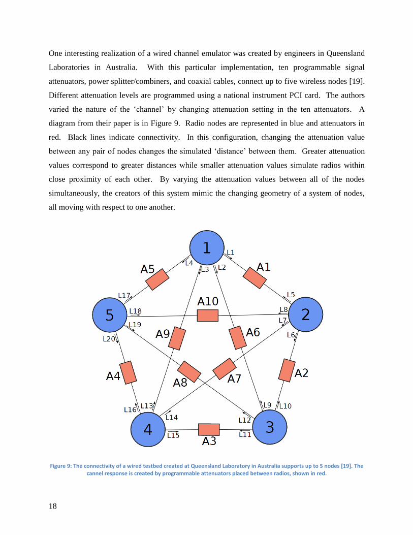
Figure 9: The connectivity of a wired testbed created at Queensland Laboratory in Australia

supports up to 5 nodes [19]. The cannel response is created by programmable attenuators

placed between radios, shown in red. ............................................................................... 17

Figure 10: 3 x 3 RF Matrix Switch [22]. Inputs are split three ways, scaled using programmable

attenuators, and recombined so that each output receives power from each of the three

inputs. ................................................................................................................................ 18

Figure 11: Elektrobit Propsim F32, radio channel emulator [24]. The F32 model has the capacity

to support as many as 32 distinct RF channels with 16 bidirectional nodes. This channel

emulator can also simulate fading..................................................................................... 20

Figure 12: Open System Interconnection Architecture (OSI) Protocol Stack, a product of the

International Organization for Standardization for characterizing layers of

communication systems [27]. ........................................................................................... 23

Figure 13: Input and Output using spread sequence (sequence shown is called Barker code), The

Data bit is transformed into Spread bits using the spread sequence. ................................ 26

Figure 14: Map of Barker Code Sequence at 1 Mbit/sec with DBPSK [29]. Each bit is modified

by an 11-bit sequence........................................................................................................ 26

Figure 15: Amplitude of DSSS Signal (Blue) vs. Narrowband Jammer (Red) before despreading

[30]. Note: signals are simplified and do not represent actual DSSS or jamming signals.

........................................................................................................................................... 27

Figure 16: Amplitude of DSSS Signal (Blue) vs. Narrowband Jammer (Red) after despreading.

The Despread signal is now at higher amplitude than the jammer’s signal...................... 27

Figure 17: Amplitude of Original Signal (Blue) vs. Processed Jammer (Red) after applying a

band-pass filter. This is the overall result of using a DSSS modulation scheme against a

narrowband interferer........................................................................................................ 28

Figure 18: Multipath signals bouncing off the environment. Signals suffer decay and arrive late

at the receiver. ................................................................................................................... 29

Figure 19: Transmitted Signal (A) with two symbols, Ideal Received Signal (B), Realistic

Received Signal (C) with multiple, decayed, overlapping received symbols from ISI. ... 30

Figure 20: Transmitted signal with high bit-rate transmission (low symbol duration) (Left).

Received signal with increased ISI (Right). ..................................................................... 30

Figure 21: Using multiple carriers to send data (FDM). Advantages: Increased data rate and

resistance to ISI using guard bands. Disadvantages: inefficient use of bandwidth. ........ 31

Figure 22: Using overlapping carriers to send data (OFDM). Advantages: greatly increased data

rate, resistance to ISI using guard bands, and efficient use of bandwidth. Disadvantages:

sensitive to carrier frequency offset or drift. ..................................................................... 32

Figure 23: Fourier transform of square, time domain signal into Sinc pulse in frequency domain.

The bandwidth is inversely related to the spacing . ............................................... 32

Figure 24: N=5 Overlapping OFDM tones. Each tone is orthogonal if the spacing between

frequencies is equal to 1/NT. Note: minimal interference at sampling points (multiples of

the symbol rate)................................................................................................................. 33

Figure 25: Two received symbols using DBPSK (Blue). Inter-Symbol Interference from

multipath signal (Red)....................................................................................................... 34

Figure 26: Two received symbols using DBPSK (Blue) and multipath signals (Red). The guard

interval avoids Inter-Symbol Interference by delaying the start of the next symbol. ....... 34

Figure 27: Two received symbols using DBPSK (Solid Blue) with a Cyclic Prefix (Dashed Blue)

added to avoid ISI. The cyclic extension is taken from the tail end of the symbol and

added to the front. ............................................................................................................. 35

Figure 28: Alternate view of the transmitted signal using Cyclic Prefix. The received signal

avoids ISI. ......................................................................................................................... 35

Figure 29: Differences between Access Point (Central Server or Point Coordination) and Ad-hoc

Networks (Mesh or Distributed Coordination). ................................................................ 36

Figure 30: IEEE 802.11 MAC Access Method using Inter-frame Spacings and the Exponential

Backoff Algorithm [14, p. 530]. ....................................................................................... 38

Figure 31: IEEE 802.11 Medium Access Control Logic [14, p. 528]. All clients will check the

medium to see if it’s idle before attempting to transmit in order to avoid collisions. ...... 39

Figure 32: Hidden Node Problem: Nodes A & C cannot hear each other and attempt to transmit

to Node B at the same time, causing a collision in the receiver of Node B. ..................... 40

Figure 33: Implementation of the RTS/CTS mechanism in 802.11 with NAV activation,

SIFS/DIFS interval, and contention window [28, p. 462]. ............................................... 41

Figure 34: Jamming Attacks at MAC & PHY Layer. Techniques are listed by intelligence

required. ............................................................................................................................ 42

Figure 35: Chart of Effectiveness vs. Efficiency of PHY (RED) and MAC (BLUE) layer attacks.

Note: All attacks are subjective. ....................................................................................... 44

Figure 36: Basic structure of analog channel emulator with key parts (A) Circulator (B) Power

Splitter/Combiner and (C) Programmable Attenuator. This diagram shows a channel

emulator that supports only three radio nodes. ................................................................. 47

Figure 42: Six-way splitter composed of cascaded two and three-way splitters. This design was

not ultimately used because it was too lossy. ................................................................... 49

Figure 43: Five two-way splitters cascaded to create a six-way splitter. This design was not

ultimately used because it did not provide enough isolation. ........................................... 50

Figure 39: Four-way splitter created from three cascaded couplers. This design is not very lossy

and provides enough isolation between paths. .................................................................. 52

Figure 40: The team decided to focus on a four node channel emulator that works from 2 to 8

GHz. Each 4-way splitter/combiner is composed of three cascaded couplers. ................ 53

Figure 41: Original ringing suppressing circuit with PCI Card (Left) and Programmable

Attenuator (Right). This circuit worked well enough when there were fewer attenuators.

........................................................................................................................................... 55

Figure 42: Final ringing suppressing circuit with added buffer capacitors placed within close

proximity to data lines, and twisted pair cables (paired with GND) for each data signal.

Note: Twisted Pair cable is not an inductor. ..................................................................... 56

Figure 43: Two-tone test setup. From left to right: Signal Generators, Isolators, Power Divider,

Device Under Test (DUT), Spectrum Analyzer. The two-tone test helps to identify third

order nonlinearities of a RF device. .................................................................................. 57

Figure 44: Two Radio Network consisting of Attenuators, Circulators, and Power Dividers.

Radios are Gumstix computers with Wi-Fi 802.11b/g. Jammers used are: USRPN210,

Signal Generators, or Noise Generators............................................................................ 61

Figure 45: Simplified diagram of connections between radio nodes and RF Channel Emulator.

Each node can vary their distance between every other node. ......................................... 62

Figure 46: Equidistant node topology. All nodes are the same distance from each other and can

exchange data with all other nodes. The jammer will approach the network at a rate of 2

meter/sec. .......................................................................................................................... 63

Figure 47: Realistic picture of Wi-Fi scenario. Three Wi-Fi emitters (Blue) within 15 meters of

another. All (Blue) nodes can exchange data at the same rate. The Emergency

Responder (Red) approaches the network and passes through while attempting to regain

spectrum. Note: not to scale. ............................................................................................ 64

Figure 48: Map of Equidistance Node scenario. Three Wi-Fi emitters (Blue) within 15 meters of

another; each can exchange data at the same rate. The Emergency Responder (Red)

approaches the network and passes through while attempting to regain spectrum. Note:

not to scale. ....................................................................................................................... 65

Figure 49: Hidden Node topology. R1 (Left) and R3 (Right) cannot communicate directly with

each other. R2 can communicate with both nodes. The jammer moves toward this

network at a rate of ~2 meters/sec. ................................................................................... 66

Figure 50: Map of Hidden Node topology. Three Wi-Fi emitters (blue, R1, R2, and R3, from left

to right). R1 cannot communicate with R3 and vice versa. The Emergency Responder

(Red) approaches the network and passes through, attempting to regain spectrum. Note:

not to scale. ....................................................................................................................... 67

Figure 51: Distant Node topology. Each node starts equidistant from other nodes and moves

away from the network in the opposite direction. The jammer approaches the network at

a rate of 2 meters/sec......................................................................................................... 68

Figure 52: Map of Distant Node topology. Three Wi-Fi emitters. R1 cannot communicate with

R3 and vice versa. The Emergency Responder (Red) approaches the network and passes

through, attempting to regain spectrum. Note: not to scale. ............................................ 69

Figure 53: Reactive Beacon Frame Injection attack on IEEE 802.11b/g. The attack injects a

manipulated beacon frame that seems as though it came from the target client.

Subsequent packets sent to that client are then using the wrong network parameters,

resulting in dropped packets and/or weakened security. .................................................. 70

Figure 54: Major attenuation states, adjusted to insertion loss, DC to 8 GHz. Insertion loss is

shown in blue. Attenuation states are relatively flat across the band. .............................. 74

Figure 55: A tone being fed through the attenuator while it steps through different attenuation

settings. The blue image on the left shows an instance of the attenuator latching the

wrong state. Note: blue/grey portion of image have been inverted to improve visibility. 75

Figure 56: Isolation between -3dB ports of two different couplers. This measurement was taken

from 2 to 8 GHz with the vector network analyzer. ......................................................... 76

Figure 57: Coupler return loss, measured from 2 to 8 GHz. Return loss for each of the -3dB

ports shown in red and blue. Return loss for sum port shown in black. .......................... 77

Figure 58: Coupler insertion loss from sum port to both -3dB ports for two different couplers.

Each of the two blue lines correspond to the loss measurement between the sum port and

one of the -3dB ports while the two red lines are the same for the other coupler measured.

This measurement was taken from 2 to 8 GHz. ................................................................ 78

Figure 59: Circulator insertion loss (top) and isolation (bottom), measured from 2 to 8 GHz with

network analyzer. .............................................................................................................. 79

Figure 60: Return loss of DiTom circulator, measured from 2 to 8 GHz with network analyzer.

Each different color represents one of the three different ports of the device. ................. 79

Figure 61: Assembled RF Analog Testbed. Radio hardware is on the far left, with circulators and

couplers towards the middle. Attenuators are on the breadboard with the PCI breakout

board on the far right......................................................................................................... 80

Figure 62: Circulators and cascaded couplers in final channel emulator configuration. The

transmit and receive sides of the circulators are circled in green. .................................... 81

Figure 63: Programmable attenuators with ringing suppressing circuit on breadboard ............... 81

Figure 64: SCB-68 NI breakout board closed (top) and open (bottom). Wires from this board are

each twisted with a ground wire and connected to the attenuators on the breadboard. .... 82

Figure 65: analysis throughout the system, based upon measured loss in each individual part at

2.4 GHz. Expected loss through the system is 21 dB. ...................................................... 84

Figure 66: Gain through the system on all twelve paths, before (left) and after calibration (right).

Colored lines correspond to 12 distinct paths through emulator. ..................................... 85

Figure 67: Spectrum of two tones combined, before entering the testbed .................................... 86

Figure 68: Two tones through the system, attenuators set to insertion loss ................................. 87

Figure 69: Two tones through the system, attenuators set to 16 dB setting ................................. 87

Figure 70: Two tones through the system, attenuators set to 31.5 dB setting .............................. 88

Figure 71: Pulse Jamming tests: Throughput vs. Pulse length & period in Two Radio (A) testbed

at 11Mbit/sec (DSSS), 9Mbit/sec (OFDM), and on the Four Radio testbed (B) at

11Mbit/sec (DSSS), 9Mbit/sec (OFDM). ......................................................................... 89

Figure 72: Sweep Jamming tests: Throughput vs. SJR & Sweep time in Two Radio testbed (A) at

11Mbit/sec (DSSS), 9Mbit/sec (OFDM), and on the Four Radio testbed (B) at 11Mbit/sec

(DSSS), 9Mbit/sec (OFDM). Results are in Mbit/sec. Signal to Jammer Ratio (SJR) and

sweep time are varied........................................................................................................ 90

Figure 73: Differences in performance of Two Radio Testbed vs. Four Radio Testbed when

subject to Sweep and Pulse waveforms. ........................................................................... 91

Figure 74: Digital Jamming tests: Throughput vs. SJR on the Two Radio testbed using

MATLAB (A) and Four Radio testbed using GNURadio (B) using 11 Mbit/sec DSSS

and 9 Mbit/sec OFDM. ..................................................................................................... 92

Figure 75: Digital Jamming tests (Corrected): Throughput vs. SJR on the Two Radio testbed

using MATLAB (A) and Four Radio testbed using MATLAB (B) using 11 Mbit/sec

DSSS and 9 Mbit/sec OFDM. ........................................................................................... 93

Figure 76: Spectrum of OFDM (9 Mbit/sec, 802.11g) signal (A) and with the addition of a

Digital jammer (B). The graph in (A) shows a typical flat, OFDM signal modulation.

The graph in (B) shows the OFDM modulation changing to a DSSS-like signal when a

Digital jammer is introduced. ........................................................................................... 94

Figure 77: Spectrum of DSSS (11 Mbit/sec, 802.11b) signal (A) and with the addition of a

Digital jammer (B). The graph in (A) shows a typical DSSS signal modulation. The

graph in (B) shows the DSSS modulation changing to an OFDM-like signal when a

Digital jammer is introduced. ........................................................................................... 95

Figure 78: Flow of data in mobile experiments. All mobile data shown in graphs are transmitted

in one direction by the prior node. .................................................................................... 96

Figure 84: Equidistant node topology in a mobile environment: Throughput vs. Time (A), and

Coordinate Grid of Radios and Jammer (B). A Digital jamming node passes between

three clients (Rx 1, 2, 3) that are equally spaced (15 meters from each node). ................ 97

Figure 80: Correlation between Jammer attenuation (distance) and Throughput between nodes

for Digital Jammer in Equidistant Node Topology. Total Network Throughput vs. Time

(A), Attenuation vs. Time of programmable attenuators (B), Throughput vs. SJR of

Digital Jammer in previous PHY layer experiment (C).................................................... 98


Coordinate Grid of Radios and Jammer (B). A Pulse jamming node passes between three

clients (Rx 1, 2, 3) that are equally spaced (15 meters from each node). ......................... 99


for Pulse Jammer in Equidistant Node Topology. Total Network Throughput vs. Time

(A), Attenuation vs. Time of programmable attenuators (B), Throughput vs. Pulse Length

vs. Pulse Period of Pulse Jammer in previous PHY layer experiment (C). .................... 100


Coordinate Grid of Radios and Jammer (B). A Sweep jamming node passes between

three clients (Rx 1, 2, 3) that are equally spaced (15 meters from each node). .............. 101


for Sweep Jammer in Equidistant Node Topology. Total Network Throughput vs. Time

(A), Attenuation vs. Time of programmable attenuators (B), Throughput vs. Sweep Time

vs. SJR of Sweep Jammer in previous PHY layer experiment (C). ................................ 102

Figure 85: Hidden node topology in a mobile environment: Throughput vs. Time (A), and


three clients (Rx 1, 2, 3) that are spaced apart laterally as to simulate a hidden node (Rx 1

and Rx 3 cannot communicate with each other). ............................................................ 104



clients (Rx 1, 2, 3) that are spaced apart laterally as to simulate a hidden node (Rx 1 and

Rx 3 cannot communicate with each other). ................................................................... 105



three clients (Rx 1, 2, 3) that are spaced apart laterally as to simulate a hidden node (Rx 1

and Rx 3 cannot communicate with each other). ............................................................ 106

Figure 88: Distant node topology in a mobile environment: Throughput vs. Time (A), and


three clients (Rx 1, 2, 3); Rx 3 is isolated and can only communicate with Rx 2 from a

longer distance. ............................................................................................................... 107



clients (Rx 1, 2, 3); Rx 3 is isolated and can only communicate with Rx 2 from a longer

distance. .......................................................................................................................... 108



three clients (Rx 1, 2, 3); Rx 3 is isolated and can only communicate with Rx 2 from a

longer distance. ............................................................................................................... 109

Figure 91: Comparison of performance among different jamming techniques in a mobile,

Equidistant node topology. Graph of Total Network Throughput vs. Time of Digital,

Pulse, and Sweep jamming. ............................................................................................ 110

Figure 92: Comparison of performance among different jamming techniques in a mobile, Hidden

node topology. Graph of Total Network Throughput vs. Time of Digital, Pulse, and

Sweep jamming. .............................................................................................................. 111

Figure 93: Comparison of performance among different jamming techniques in a mobile, Distant

node topology. Graph of Total Network Throughput vs. Time of Digital, Pulse, and

Sweep jamming. .............................................................................................................. 112

Figure 94: Effects on throughput from Digital Jamming. Results from published work [7] (top),

results from two node testbed (bottom). ......................................................................... 122

Figure 95: Effects on throughput from Pulse Jamming. Results from published work [7] (left),

results from two node testbed (right). ............................................................................. 123

Figure 96: Effects on throughput from Sweep Jamming. Results from published work [34] (left),

results from two node testbed (right). ............................................................................. 123

List of Tables

Table 1: Project deliverables are divided into thresholds and objectives. Deliverables pertain to

both the channel emulator and the Wi-Fi DoS portions of the project ............................... 4

Table 2: Comparison of different channel emulators and testbeds. Testbeds can be wired or

wireless and include a variety of different mechanisms for motion emulation. ............... 21

Table 3: Definitions of Inter-frame Spacings and their role in the MAC Layer [14]. .................. 37

Table 4: PHY Layer Jamming Definitions. .................................................................................. 42

Table 5: MAC Layer Jamming Definitions. ................................................................................. 43

Table 6: Design attempts for RF channel emulator. The two original design attempts did not meet

specifications..................................................................................................................... 51

Table 7: The testbed was channelized into two separate frequency bands, 30 MHz - 3 GHz and 2

- 8 GHz, with two separate sets of parts. .......................................................................... 52

Table 8: List of equipment used in PHY layer attacks by name, model, and specifications. ....... 59

Table 9: The twelve 'paths' in the channel emulator. Each path has its own programmable

attenuator........................................................................................................................... 83

Table 10: List of 802.11 Standards [14]. .................................................................................... 121

List of Acronyms

ACK Acknowledgement AP Access Point AWGN Additive White Gaussian Noise DBPSK Differential Binary Phase Shift Keying BER Bit Error Rate BPSK Binary Phase Shift Keying BW Bandwidth CDMA Code Division Multiple Access CSMA/CA Carrier Sense Multiple Access / Collision Avoidance CTS Clear to Send dB Decibel DCF Distributed Coordinate Function DIFS Distributed Coordinate Function Inter-Frame Spacing DoS Denial of Service DSSS Direct Sequence Spread Spectrum FDM Frequency Division Multiplexing FHSS Frequency Hopping Spread Spectrum FTP File Transfer Protocol HTTP Hyper-Text Transfer Protocol ICI Inter-Carrier Interference IEEE Institute of Electrical and Electronics Engineer IFS Inter-Frame Spacing IMAP Internet Message Access Protocol IP Internet Protocol ISI Inter-Symbol Interference ISO International Standards Organization JSR Jammer to Signal Ratio LAN Local Area Network MAC Medium Access Control MIMO Multiple Input Multiple Output NAV Network Allocation Vector NFS Network File System OFDM Orthogonal Frequency Division Multiplexing OSI Open Systems Interconnection PCF Point Coordinate Function PHY Physical PIFS Point Coordinate Function Inter-Frame Spacing PLCP PHY Layer Convergence Protocol PMD PHY Layer Medium Dependent Protocol POP Post Office Protocol RF Radio Frequency RTS Request to Send SIFS Short Inter-Frame Spacing SJR Signal to Jammer Ratio SMA Sub-Miniature Version A

SMTP Simple Mail Transfer Protocol SNR Signal to Noise Ratio TCP Transmission Control Protocol UDP User Datagram Protocol UHF Ultra-High Frequency USRP Universal Software Radio Peripheral WEP Wired Equivalency Privacy WLAN Wireless Local Area Network WPA Wi-Fi Protected Access

1

1 Introduction

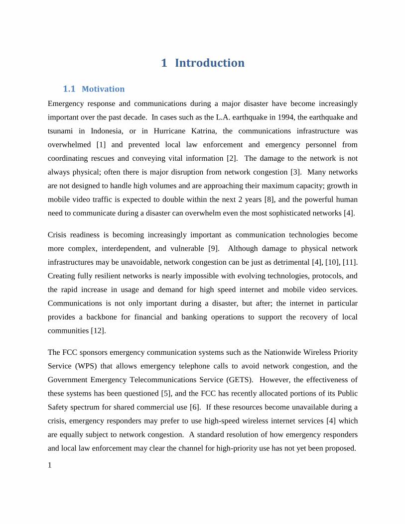
1.1 Motivation

Emergency response and communications during a major disaster have become increasingly

important over the past decade. In cases such as the L.A. earthquake in 1994, the earthquake and

tsunami in Indonesia, or in Hurricane Katrina, the communications infrastructure was

overwhelmed [1] and prevented local law enforcement and emergency personnel from

coordinating rescues and conveying vital information [2]. The damage to the network is not

always physical; often there is major disruption from network congestion [3]. Many networks

are not designed to handle high volumes and are approaching their maximum capacity; growth in

mobile video traffic is expected to double within the next 2 years [8], and the powerful human

need to communicate during a disaster can overwhelm even the most sophisticated networks [4].

Crisis readiness is becoming increasingly important as communication technologies become

more complex, interdependent, and vulnerable [9]. Although damage to physical network

infrastructures may be unavoidable, network congestion can be just as detrimental [4], [10], [11].

Creating fully resilient networks is nearly impossible with evolving technologies, protocols, and

the rapid increase in usage and demand for high speed internet and mobile video services.

Communications is not only important during a disaster, but after; the internet in particular

provides a backbone for financial and banking operations to support the recovery of local

communities [12].

The FCC sponsors emergency communication systems such as the Nationwide Wireless Priority

Service (WPS) that allows emergency telephone calls to avoid network congestion, and the

Government Emergency Telecommunications Service (GETS). However, the effectiveness of

these systems has been questioned [5], and the FCC has recently allocated portions of its Public

Safety spectrum for shared commercial use [6]. If these resources become unavailable during a

crisis, emergency responders may prefer to use high-speed wireless internet services [4] which

are equally subject to network congestion. A standard resolution of how emergency responders

and local law enforcement may clear the channel for high-priority use has not yet been proposed.

2

In this paper we introduce the problems of network congestion facing the future of

communications during a crisis and the availability of this resource to emergency responders.

Our team presents a prototype testbed, including a real-time channel emulator, and focuses on

demonstrating a practical solution to network congestion in an emulated, mobile environment

using commercial 802.11 Wi-Fi devices and programmable radios.

1.2 Problem Statements

There is currently not enough exclusive spectrum for emergency responders to reliably

communicate during a crisis. Popularity and demand in wireless communication has surged in

recent years, increasing susceptibility to network congestion. Additionally, recent laws

regulating public safety spectrum for commercial use suggest it may be especially vulnerable to

congestion. This problem presents a key question that frames our project:

How can we efficiently and effectively clear network congestion to reallocate the spectrum for

emergency responders?

In order to address this question, we examine the solution space for ownership in a contested

communications environment.

1.3 Proposed Solution

Our team proposes a denial of service (DoS) technique that is capable of removing Wi-Fi

interferers from the channel so that authorized personnel can regain this resource. If effective,

this method could be used by emergency responders to efficiently and effectively clear congested

networks to re-establish communications by authorized personnel. However, experimenting with

and validating this technique across open air-waves would disrupt user services and violate FCC

regulations; thus a computer controlled testbed, including a real-time RF channel emulator that

uses commercially available Wi-Fi radios and a Universal Software Radio Peripheral (USRP),

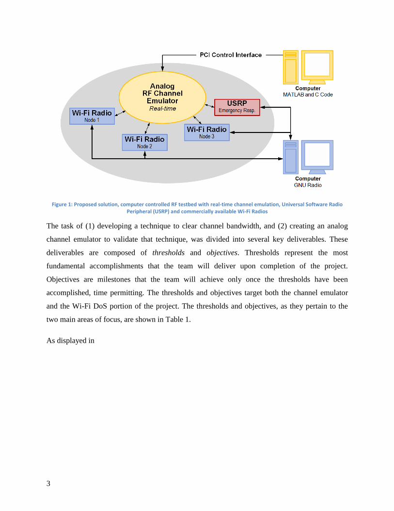
will be designed for this purpose. The basic structure of this testbed solution is shown in Figure

1.

3

Figure 1: Proposed solution, computer controlled RF testbed with real-time channel emulation, Universal Software Radio Peripheral (USRP) and commercially available Wi-Fi Radios

The task of (1) developing a technique to clear channel bandwidth, and (2) creating an analog

channel emulator to validate that technique, was divided into several key deliverables. These

deliverables are composed of thresholds and objectives. Thresholds represent the most

fundamental accomplishments that the team will deliver upon completion of the project.

Objectives are milestones that the team will achieve only once the thresholds have been

accomplished, time permitting. The thresholds and objectives target both the channel emulator

and the Wi-Fi DoS portion of the project. The thresholds and objectives, as they pertain to the

two main areas of focus, are shown in Table 1.

As displayed in

4

Table 1, the most basic requirements for the channel emulator are: support for 2 to 8 GHz of

bandwidth, variable attenuators to simulate changing geometries, and support for four radio

nodes. This channel emulator will be built and tested by completion of the project. Time

allowing, this testbed can be scaled up to support six radios on a 30 MHz to 8 GHz bandwidth.

If building this enhanced testbed is not feasible in the limited time frame, the team will present

the MIT Lincoln Laboratories mentors with basic plans, including preliminary parts lists, for the

six node testbed that supports a 30 MHz to 8 GHz bandwidth. Components of the channel

emulator and the assembled system will be tested thoroughly to ensure that specifications have

been met.

5

Table 1: Project deliverables are divided into thresholds and objectives. Deliverables pertain to both the channel emulator and the Wi-Fi DoS portions of the project

Thresholds Objectives

Channel Emulator Support for 4 nodes. Support for 6 nodes.

Wideband (2-8 GHz). Coverage for 30 MHz to 8 GHz.

Real-time (variable attenuator to simulate

changing nodal geometries).

Wi-Fi DoS Attack Validate the channel emulator by

repeating existing Wi-Fi attacks.

“Reactive Beacon Frame Injection”

attack in the MAC layer.

Examine results of the same Wi-Fi attacks

using different mobile scenarios.

In order to meet threshold requirements in the Wi-Fi DoS portion of the project, known PHY

(Physical) layer jamming techniques will be repeated and documented, first on a simple two

radio network for validation, then on the channel emulator. Repeating known attacks and

validating consistency in the results is an important way to ensure functionality in the channel

emulator. Once the accuracy of the testbed has been confirmed, the mobility feature of the

channel emulator will be used to repeat the same PHY layer attacks in three different mobile

configurations of nodes. Lastly, time permitting; a MAC (Medium Access Control) layer attack

will be attempted on the channel emulator. The proposed MAC layer attack is called “Reactive

Beacon Frame Injection”, where beacon frames are injected with false information, intended to

disrupt transmissions between other clients.

1.4 Report Organization

This report will document background information pertaining to the project topic, the process

and methods, and subsequently the results, discussion, the conclusion. Chapter two will be an

overview of RF channels, wireless networks, and Wi-Fi security. The important attributes of an

RF channel and different ways that these characteristics have been recreated in various types of

channel emulators will be covered. In addition, wireless network basics and Wi-Fi protocol and

6

security will be outlined. Chapter 3 will detail the methods used to design, build, and test the

analog channel emulator along with the techniques for both PHY and MAC layer jamming.

Finally, the results of the group’s measurements on the testbed, PHY layer jamming, and the

Reactive Beacon Frame Injection will be presented in chapter 4, discussed in chapter 5, and put

into context in chapter 6.

7

2 Overview of RF Channels,

Wireless Networks, and Security

In order to successfully build an analog RF channel emulator and demonstrate a DoS attack,

background research was necessary in many areas. Our team isolated several key areas for

further investigation. In particular, the team was interested in the different characteristics that

define realistic RF channels and how these conditions can be, and have been, recreated in

different types of channel emulators and testbeds. The ability to create a realistic analog channel

emulator depends upon a thorough understanding of the RF channel and how it has been

simulated by researchers in the past. An in-depth knowledge of Wi-Fi, in particular the MAC

and PHY layers of IEEE 802.11, is instrumental in isolating and exploiting any weaknesses. In

order to create a new DoS attack, the team also conducted a literature review of different types of

Wi-Fi denial of service attacks that have already been tested. This chapter will review these

topics as they pertain to our project goals.

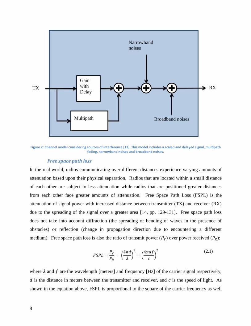
2.1 The RF Channel

In an ideal world, RF power transmitted would arrive at the receiver unscathed. In reality, the

signal is scaled, delayed, and distorted in a variety of ways. Understanding all of the factors that

can impact signal integrity is crucial to successful radio communications. Being able to simulate

and recreate some of these characteristics and effects to allow for accurate testing is of equal

importance. This section describes the basic attribute of an RF channel and then reviews some

of the different techniques for recreating these conditions for wireless network testing.

Important aspects of RF channel

An RF channel describes the path between a transmitter and a receiver. In an ‘ideal’ channel, the

signal is the same at the receiver as it is at the transmitter with the exception of a small delay and

attenuation. However, this model of a channel neglects some of the many other types of

interferences and distortions that could alter or corrupt the signal on its way the receiver [13, p.

11]. Some of these impairments include multipath, signal fading, and various noise sources.

The diagram below shows one channel model that includes some of the different types of

distortion and interference.

8

Figure 2: Channel model considering sources of interference [13]. This model includes a scaled and delayed signal, multipath fading, narrowband noises and broadband noises.

Free space path loss

In the real world, radios communicating over different distances experience varying amounts of

attenuation based upon their physical separation. Radios that are located within a small distance

of each other are subject to less attenuation while radios that are positioned greater distances

from each other face greater amounts of attenuation. Free Space Path Loss (FSPL) is the

attenuation of signal power with increased distance between transmitter (TX) and receiver (RX)

due to the spreading of the signal over a greater area [14, pp. 129-131]. Free space path loss

does not take into account diffraction (the spreading or bending of waves in the presence of

obstacles) or reflection (change in propagation direction due to encountering a different

medium). Free space path loss is also the ratio of transmit power ( ) over power received ( ):

(2.1)

where and are the wavelength [meters] and frequency [Hz] of the carrier signal respectively,

is the distance in meters between the transmitter and receiver, and is the speed of light. As

shown in the equation above, FSPL is proportional to the square of the carrier frequency as well

RX

Gain

with

Delay

Multipath

Narrowband

noises

Broadband noises

TX

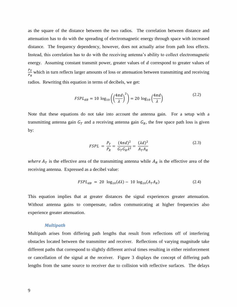
9

as the square of the distance between the two radios. The correlation between distance and

attenuation has to do with the spreading of electromagnetic energy through space with increased

distance. The frequency dependency, however, does not actually arise from path loss effects.

Instead, this correlation has to do with the receiving antenna’s ability to collect electromagnetic

energy. Assuming constant transmit power, greater values of correspond to greater values of

which in turn reflects larger amounts of loss or attenuation between transmitting and receiving

radios. Rewriting this equation in terms of decibels, we get:

(2.2)

Note that these equations do not take into account the antenna gain. For a setup with a

transmitting antenna gain and a receiving antenna gain , the free space path loss is given

by:

(2.3)

is the effective area of the transmitting antenna while is the effective area of the

receiving antenna. Expressed as a decibel value:

(2.4)

This equation implies that at greater distances the signal experiences greater attenuation.

Without antenna gains to compensate, radios communicating at higher frequencies also

experience greater attenuation.

Multipath

Multipath arises from differing path lengths that result from reflections off of interfering

obstacles located between the transmitter and receiver. Reflections of varying magnitude take

different paths that correspond to slightly different arrival times resulting in either reinforcement

or cancellation of the signal at the receiver. Figure 3 displays the concept of differing path

lengths from the same source to receiver due to collision with reflective surfaces. The delays

10

and signal magnitude associated with each of the paths in the diagram will determine, to some

extent, the quality of the signal received at receiver.

Figure 3: Obstacles cause electromagnetic waves to reflect and travel different paths of varying lengths. The red path, path 1, is the line of site path while the blue path, path 2, is the result of reflected signal power. Signal power traveling path two

travels a greater distance and thus experiences greater delay. The sum of the power from both paths is a signal that is distorted due to multipath effects.

In the case of the diagram shown above, the signal power at the receiver is composed of power

from the line of site path (path 1) and power from the reflected path (path 2). The graph to the

right shows what the waveforms might look like at the receiver. Because power travelling path 2

(Blue) travels a greater distance, it arrives at the receiver some time delay after signal power

traveling along path 1 (Red) arrives. As a result, the sum of the two received signals (Green) is a

slightly distorted version of the original signal. This scenario displays the concept of multipath,

but in reality, many more paths can exist creating even greater distortion. The signal at the

receiver in any given time can be expressed as the sum of the scaled and delayed reflections

arriving at the receiving radio [13, p. 62]. If s(t) represents the transmitted signal then the

received signal rx(t) is given by:

(2.5)

where is the magnitude of the signal is the time delay, and N is the total number of delays.

Physically, this means that the received signal, as shown in Figure 2Figure 3, is composed of not

only the power from the line of site propagation but also signal power from any reflected path

11

that might exist. Electromagnetic energy propagating along the reflected paths arrive some time

delay after the line of site propagation arrives. This time delay is based upon the length of the

path traveled. Summing all of the different scaled and delayed reflections that arrive at the

receiver can result in a signal that is distorted to some degree. If this distortion is severe enough,

it can interfere with signal integrity.

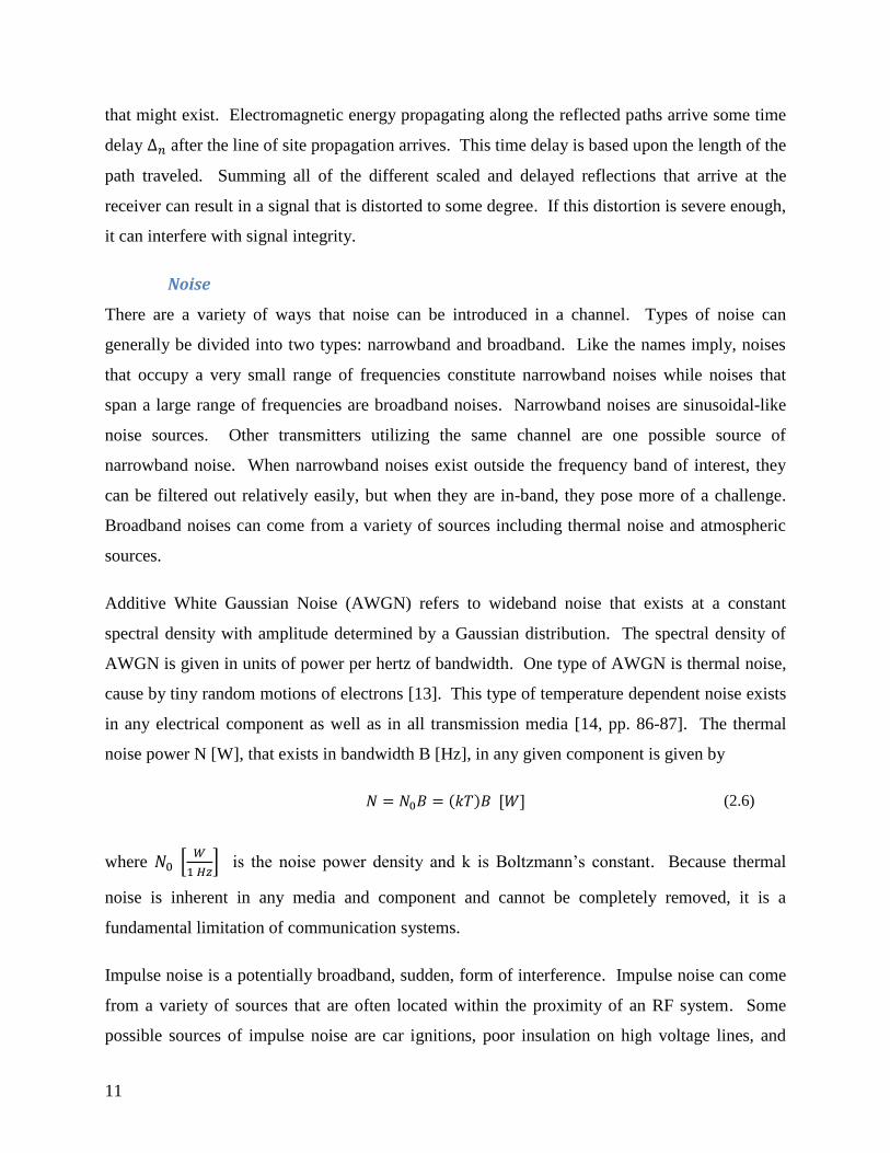
Noise

There are a variety of ways that noise can be introduced in a channel. Types of noise can

generally be divided into two types: narrowband and broadband. Like the names imply, noises

that occupy a very small range of frequencies constitute narrowband noises while noises that

span a large range of frequencies are broadband noises. Narrowband noises are sinusoidal-like

noise sources. Other transmitters utilizing the same channel are one possible source of

narrowband noise. When narrowband noises exist outside the frequency band of interest, they

can be filtered out relatively easily, but when they are in-band, they pose more of a challenge.

Broadband noises can come from a variety of sources including thermal noise and atmospheric

sources.

Additive White Gaussian Noise (AWGN) refers to wideband noise that exists at a constant

spectral density with amplitude determined by a Gaussian distribution. The spectral density of

AWGN is given in units of power per hertz of bandwidth. One type of AWGN is thermal noise,

cause by tiny random motions of electrons [13]. This type of temperature dependent noise exists

in any electrical component as well as in all transmission media [14, pp. 86-87]. The thermal

noise power N [W], that exists in bandwidth B [Hz], in any given component is given by

(2.6)

where

is the noise power density and k is Boltzmann’s constant. Because thermal

noise is inherent in any media and component and cannot be completely removed, it is a

fundamental limitation of communication systems.

Impulse noise is a potentially broadband, sudden, form of interference. Impulse noise can come

from a variety of sources that are often located within the proximity of an RF system. Some

possible sources of impulse noise are car ignitions, poor insulation on high voltage lines, and

12

lightning [15]. Analog signals are less vulnerable to impulse noise than digital signals. For

example, voice transmission can be corrupted but not always in a way that cripples the

information. Although disruption can be heard, the information is still intelligible [14, p. 88].

Digital signals, however, can be greatly disrupted by a short burst of energy because of the high

data rate. Impulse noise can cause burst errors, defined by IEEE as a collection of consecutive

bits where no more than a given amount of bits is received correctly and the first and last bits in

the string are received in error.

As shown in Figure 2, broadband and narrowband noise is combined with the signal additively.

A noisy time domain signal also appears noisy in the frequency domain. The frequency domain

is a useful way to visualize noise because it shows the exact location in frequency of the different

noise sources.

Figure 4: (A) Noiseless time domain 60Hz signal. (B) Noiseless 60 Hz frequency domain signal. (C) 60 Hz time domain signal with AWGN (Blue) and noiseless 60Hz time domain signal. (D) Noisy 60 Hz signal in the frequency domain, the noise floor is

shown in red.

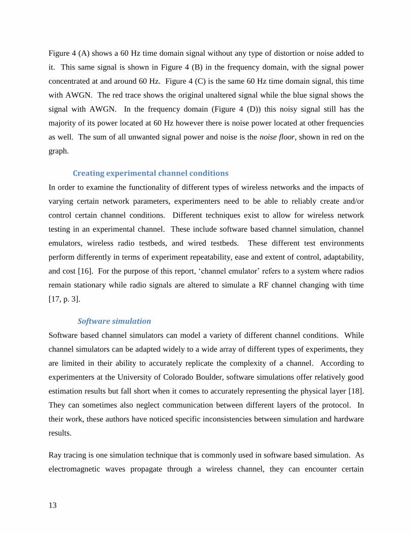
13

Figure 4 (A) shows a 60 Hz time domain signal without any type of distortion or noise added to

it. This same signal is shown in Figure 4 (B) in the frequency domain, with the signal power

concentrated at and around 60 Hz. Figure 4 (C) is the same 60 Hz time domain signal, this time

with AWGN. The red trace shows the original unaltered signal while the blue signal shows the

signal with AWGN. In the frequency domain (Figure 4 (D)) this noisy signal still has the

majority of its power located at 60 Hz however there is noise power located at other frequencies

as well. The sum of all unwanted signal power and noise is the noise floor, shown in red on the

graph.

Creating experimental channel conditions

In order to examine the functionality of different types of wireless networks and the impacts of

varying certain network parameters, experimenters need to be able to reliably create and/or

control certain channel conditions. Different techniques exist to allow for wireless network

testing in an experimental channel. These include software based channel simulation, channel

emulators, wireless radio testbeds, and wired testbeds. These different test environments

perform differently in terms of experiment repeatability, ease and extent of control, adaptability,

and cost [16]. For the purpose of this report, ‘channel emulator’ refers to a system where radios

remain stationary while radio signals are altered to simulate a RF channel changing with time

[17, p. 3].

Software simulation

Software based channel simulators can model a variety of different channel conditions. While

channel simulators can be adapted widely to a wide array of different types of experiments, they

are limited in their ability to accurately replicate the complexity of a channel. According to

experimenters at the University of Colorado Boulder, software simulations offer relatively good

estimation results but fall short when it comes to accurately representing the physical layer [18].

They can sometimes also neglect communication between different layers of the protocol. In

their work, these authors have noticed specific inconsistencies between simulation and hardware

results.

Ray tracing is one simulation technique that is commonly used in software based simulation. As

electromagnetic waves propagate through a wireless channel, they can encounter certain

14

environmental characteristics and objects that cause the wave to change direction. Ray tracing is

a method that approximates the traveling wave as a set of small ‘rays’ that travel in a straight

lines across small sections of distance. Each ray is moved in a straight line over that small

distance and then the direction of propagation is calculated again for the next small section. For

a radio channel, this method can be used for simulating the effects of multipath. For an isotropic

source, for example, radiation could be modeled as a large amount of rays coming directly out of

the source. When one of these rays encounters a reflective surface, it changes direction

accordingly. The sum of rays that arrive at the receiver at any given time is the resulting

distorted signal. While software based simulation is extremely useful for some types of testing,

testbeds that connect to actual radio hardware offer additional accuracy in the PHY layer.

Wireless testbeds

In the real world, radios generally communicate over a given distance, through air, using

antennas. This real world scenario is shown in the top part of Figure 5. Testing radios in this

type of setting requires large amounts of space and is often complicated, difficult to control, and

not very repeatable. Furthermore, proper permissions need to be obtained from the FCC in order

to use certain bandwidths at certain broadcast powers. For this reason, this type of testing is not

always feasible and alternatives in a controlled laboratory setting are needed. In the context of

this report, wireless radio testbeds refer to testbeds that involve an arrangement of nodes where

physical antennas remain as part of the system. This is an important distinction from wired

testbeds where antennas are removed and replaced with coaxial cables. Both types of testbeds

along with the real world scenario that they represent are portrayed in Figure 5.

Real world distances can be mimicked in a much smaller laboratory environment by placing

attenuators between the output of the radio and the antennas as shown in the middle section of

Figure 5. This causes the magnitude of the transmitted and received signal to be smaller, as it

would be if the radios were communicating over a greater distance.

15

`

Figure 5: The real world radio communications scenario, shown on top, can be modeled using a wireless, miniaturized, configuration with attenuators (middle). The concept of a wired testbed is at the bottom of the image. A wired testbed

involves radios that are connected to each other using coaxial cable and RF components, like the attenuator shown, to model channel response.

The channel can be further modified by introducing noise generators [19]. Noise generators, or

‘noise bricks’, give experimenters another degree of control over the channel that is being

simulated. An RF noise generator is shown below in Figure 6.

Figure 6: Noise generators can be used to add noise to a channel emulator. This noise generator, or ‘noise brick’, is manufactured by Noisecom Incorporated.

16

While wireless testbeds can sometimes create useful and realistic experimental conditions,

implementing them comes with some unique challenges, such as achieving repeatability [20].

Aspects like fading and external sources of interference tend to vary with time and are extremely

difficult to control, even in the laboratory. In some wireless testbeds, system mobility can be

achieved only through actually physically moving nodes. For example, the Miniaturized

Wireless Network Testbed (MiNT), created by researchers at Stony Brook University, achieves

node mobility by mounting nodes on iRobot’s Roomba, a vacuum cleaning robot.

One of the better known wireless network testbeds is the Open Access Research Testbed for

Next-Generation Wireless Networks (ORBIT), located at Rutgers University. This testbed is

accessible to members of the research community who can write their own code to run custom

experiments remotely on the radio grid. ORBIT currently houses 400 radio nodes indoors. A

picture of some of these nodes is in Figure 7.

Figure 7: The indoor testing facility at Rutgers University [21] is open for use to members of the research community who write their own code. Each yellow box is one of 400 stationary radio nodes.

Despite the impressive utility of ORBIT, it does not exist without limitation. For example, all

nodes in ORBIT are stationary. For this reason, the only way to change network topology is by

either including or excluding specific nodes from the configuration. Orbit also faces the same

challenges as any other wireless testbed in terms of controlling experiment reproducibility.

A smaller scale and less expensive testbed called The Emulated Wireless Ad Hoc Network

Testbed (EWANT) was created at the University of Colorado at Boulder [18]. This testbed is

17

significantly scaled down in size and is capable of simulating node mobility. Attenuators

situated between antennas and Wi-Fi cards allow a large scale setup to exist in a much smaller

location. In order to create mobility, the RF signal is multiplexed four ways and terminated in

four separate antennas. A switch enables selection between the four unique antenna outputs.

The antennas in EWANT are arranged in different configuration on a metallic tabletop with

holes as shown in Figure 8. Antennas can be moved to different holes to represent different node

geometries.

Figure 8: In the EWANT testbed, antennas can be rearranged on metallic table top with holes to create unique geometries. By switching between antennas, mobility can be emulated.

Because each radio is connected to a switch that can select from one of four differently placed

antennas, limited mobility can be simulated. When the switch selects a different transmitting

antenna, it is as if the radio has ‘moved’, albeit rather suddenly.

Wired Testbeds

Wired testbed configurations generally involve physically connecting radios with a network of

coax cables and a combination of passive and active components that create realistic and

controllable channel conditions. The key benefit to wired testbeds is their repeatability. Unlike

wireless testbeds, where many of the external conditions are difficult to control, wired testbeds

exist in a smaller, much more controllable, and thus far more repeatable environment. Despite

the high costs of creating an adaptable wired testbed, they can offer a repeatable and realistic test

setting.

18

One interesting realization of a wired channel emulator was created by engineers in Queensland

Laboratories in Australia. With this particular implementation, ten programmable signal

attenuators, power splitter/combiners, and coaxial cables, connect up to five wireless nodes [19].

Different attenuation levels are programmed using a national instrument PCI card. The authors

varied the nature of the ‘channel’ by changing attenuation setting in the ten attenuators. A

diagram from their paper is in Figure 9. Radio nodes are represented in blue and attenuators in

red. Black lines indicate connectivity. In this configuration, changing the attenuation value

between any pair of nodes changes the simulated ‘distance’ between them. Greater attenuation

values correspond to greater distances while smaller attenuation values simulate radios within

close proximity of each other. By varying the attenuation values between all of the nodes

simultaneously, the creators of this system mimic the changing geometry of a system of nodes,

all moving with respect to one another.

Figure 9: The connectivity of a wired testbed created at Queensland Laboratory in Australia supports up to 5 nodes [19]. The cannel response is created by programmable attenuators placed between radios, shown in red.

19

A similar testbed, called MeshTest, was created by the Laboratory for Telecommunications

Sciences to support as many as twelve nodes [20]. Researchers who created this testbed used an

RF matrix switches to route and attenuate signals between the different nodes. An example of a

3 x 3 RF matrix switch is shown in Figure 10, with three inputs, three outputs, and nine

attenuators.

Figure 10: 3 x 3 RF Matrix Switch [22]. Inputs are split three ways, scaled using programmable attenuators, and recombined so that each output receives power from each of the three inputs.

The RF matrix switch shown in Figure 10 works by splitting the power from each input three

ways. Each RF path is then connected to a programmable attenuator and power from each of the

three inputs is combined into each of the three outputs using a 3-way divider to combine the

signals. The programmable attenuators allow the user to control the magnitude of each input at

20

each of the three outputs. In MeshTest, this configuration allows the user to control the signal

power between all of the radio pairs.

For this type of connectivity, the number of attenuators needed is equivalent to the number of

inputs multiplied by the number of outputs. For MeshTest, programmable attenuators supported

attenuation values from 0-127 dB. According to authors, the values programmed into the

attenuators can be expressed in a matrix , where the number of rows and columns is the same as

the number of nodes. The multiplicative attenuation from node i to node j is given by element

in the matrix . Different values in matrix L represent different physical configurations and

distances between radios in the channel. Adjusting the attenuator values rapidly can mimic

channel conditions for a mobile group of nodes. To increase usability, creators of this testbed

developed a GUI that allows the user to define starting, interim, and ending locations for the

nodes as well as certain timing intricacies.

A second class of wired channel emulators utilize FPGA based signal processing rather than

programmable attenuators to simulate motion and to mimic more complicated channel

conditions. These types of channel emulators can model multipath, fading, as well as path loss.

Radios that comprise a network under test are plugged directly into this device. The RF signal

from each of these nodes is then downconverted and sampled by an ADC. The resulting signals

are then sent to a channel simulating FPGA board where signals can be attenuated, filtered, and

combined. Finally, the signals pass through a DAC, are upconverted, and sent to recipient

radios. The CMU Wireless Emulator is one example of this type of channel emulator from

academia [23]. This emulator is capable of supporting up to 15 nodes with 210 independent

channels. In this case, the channel simulator board is a Virtex 2 Pro FPGA. This emulator is

somewhat similar to the commercially available Elektrobit Propsim F32 channel emulator shown

in Figure 11.

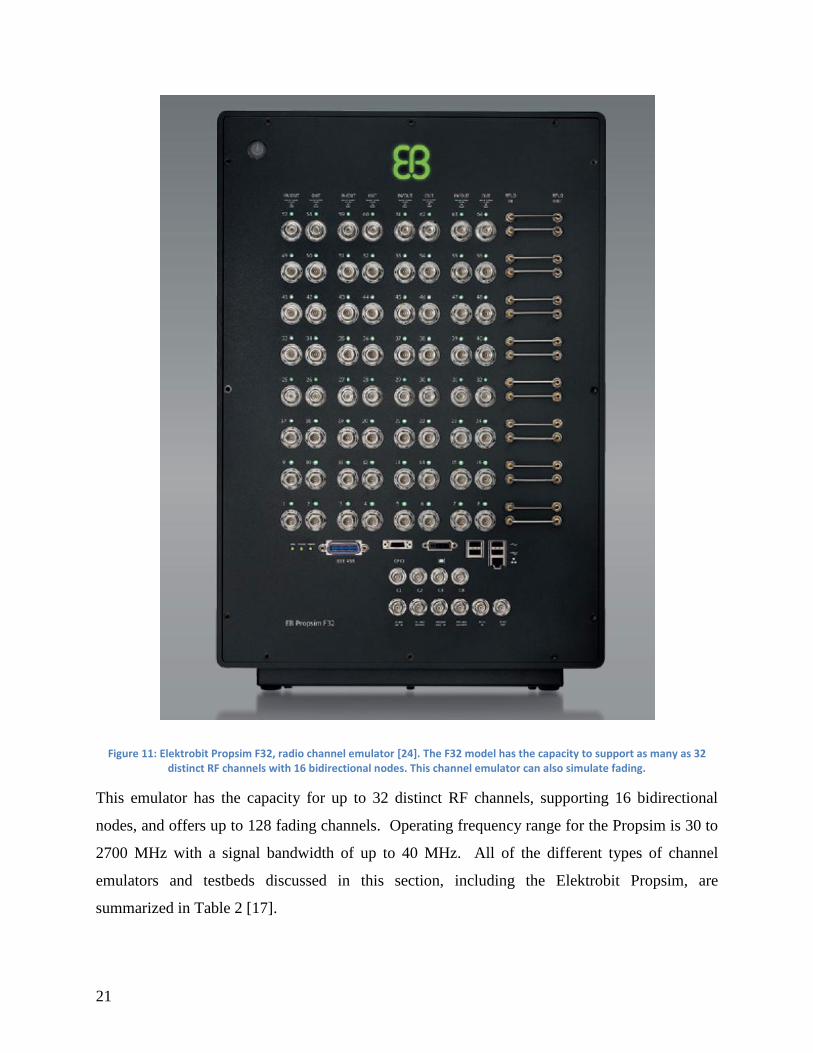
21

Figure 11: Elektrobit Propsim F32, radio channel emulator [24]. The F32 model has the capacity to support as many as 32 distinct RF channels with 16 bidirectional nodes. This channel emulator can also simulate fading.

This emulator has the capacity for up to 32 distinct RF channels, supporting 16 bidirectional

nodes, and offers up to 128 fading channels. Operating frequency range for the Propsim is 30 to

2700 MHz with a signal bandwidth of up to 40 MHz. All of the different types of channel

emulators and testbeds discussed in this section, including the Elektrobit Propsim, are

summarized in Table 2 [17].

22

Table 2: Comparison of different channel emulators and testbeds. Testbeds can be wired or wireless and include a variety of different mechanisms for motion emulation.

Name Mobility

Mechanism

Wireless

or Wired

Maximum

Number of

Nodes

Wireless Medium

Modeling

MiNT (Miniaturized

Wireless Network

Testbed)

Robots

(iRobot’s

Roomba)

Wireless 8 IEEE 802.11

ORBIT (Open-access

Research Testbed for

Next-Generation Wireless

Networks)

Antenna

switching

Wireless 400 IEEE 802.11,

Bluetooth,

EWANT (Emulated

Wireless Ad-hoc Network

Testbed)

Antenna

switching

Wireless 4 IEEE 802.11

MeshTest (Laboratory-

based wireless testbed for

large topologies)

Programmable

attenuators

Wired 12 IEEE 802.11

Queensland Lab Testbed

(For wireless mesh

networks [13])

Programmable

attenuators

Wired 5 IEEE 802.11

CMU Wireless Emulator FPGA channel

simulator board

Wired 15 (210

independent

channels)

IEEE 802.11 (2.4

GHz, 90 MHz

BW)

Elektrobit Propsim F32 FPGA Wired 16 (128

fading

channels)

30 to 2700 MHz

(40 MHz BW)

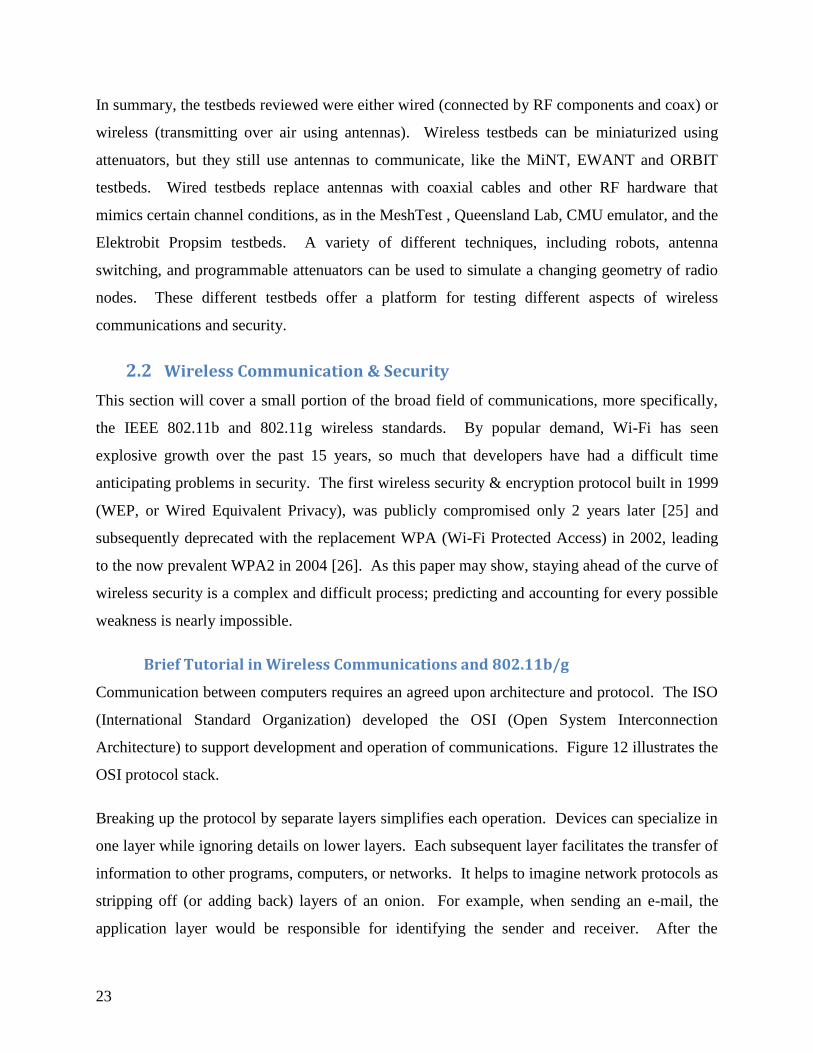
23

In summary, the testbeds reviewed were either wired (connected by RF components and coax) or

wireless (transmitting over air using antennas). Wireless testbeds can be miniaturized using

attenuators, but they still use antennas to communicate, like the MiNT, EWANT and ORBIT

testbeds. Wired testbeds replace antennas with coaxial cables and other RF hardware that

mimics certain channel conditions, as in the MeshTest , Queensland Lab, CMU emulator, and the

Elektrobit Propsim testbeds. A variety of different techniques, including robots, antenna

switching, and programmable attenuators can be used to simulate a changing geometry of radio

nodes. These different testbeds offer a platform for testing different aspects of wireless

communications and security.

2.2 Wireless Communication & Security

This section will cover a small portion of the broad field of communications, more specifically,

the IEEE 802.11b and 802.11g wireless standards. By popular demand, Wi-Fi has seen

explosive growth over the past 15 years, so much that developers have had a difficult time

anticipating problems in security. The first wireless security & encryption protocol built in 1999

(WEP, or Wired Equivalent Privacy), was publicly compromised only 2 years later [25] and

subsequently deprecated with the replacement WPA (Wi-Fi Protected Access) in 2002, leading

to the now prevalent WPA2 in 2004 [26]. As this paper may show, staying ahead of the curve of

wireless security is a complex and difficult process; predicting and accounting for every possible

weakness is nearly impossible.

Brief Tutorial in Wireless Communications and 802.11b/g

Communication between computers requires an agreed upon architecture and protocol. The ISO

(International Standard Organization) developed the OSI (Open System Interconnection

Architecture) to support development and operation of communications. Figure 12 illustrates the

OSI protocol stack.

Breaking up the protocol by separate layers simplifies each operation. Devices can specialize in

one layer while ignoring details on lower layers. Each subsequent layer facilitates the transfer of

information to other programs, computers, or networks. It helps to imagine network protocols as

stripping off (or adding back) layers of an onion. For example, when sending an e-mail, the

application layer would be responsible for identifying the sender and receiver. After the

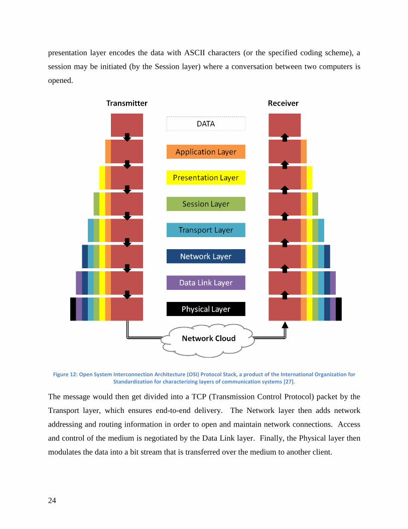
24

presentation layer encodes the data with ASCII characters (or the specified coding scheme), a

session may be initiated (by the Session layer) where a conversation between two computers is

opened.

Figure 12: Open System Interconnection Architecture (OSI) Protocol Stack, a product of the International Organization for Standardization for characterizing layers of communication systems [27].

The message would then get divided into a TCP (Transmission Control Protocol) packet by the

Transport layer, which ensures end-to-end delivery. The Network layer then adds network

addressing and routing information in order to open and maintain network connections. Access

and control of the medium is negotiated by the Data Link layer. Finally, the Physical layer then

modulates the data into a bit stream that is transferred over the medium to another client.

25

The IEEE 802 standard, built upon the OSI model, provided a framework for wireless

communication, which requires a slightly modified protocol to account for mobility and security.

Motivation for wireless communication standards began in the 1980’s to support factory

environments [28]. The IEEE 802.11 standard became the first and only WLAN (Wireless Local

Area Network) standard to successfully secure a market. This 2,500 page document specifies the

protocol for PHY (Physical: RF and modulation schemes) and MAC (Medium Access Control)

layers of a communication architecture.

The main objectives of the 802.11 standard were to provide a mechanism that could allow

overlapping networks, include conditions that handle interference from radios and microwave

ovens, eliminate “hidden terminal” problems, support time-bounded services, and maintain

privacy and secure access [28]. Table 10 in the Appendix lists 802.11 standards and their scope.

The following list describes layers implemented in the 802.11 protocol stack [14]:

Upper layers are not defined in 802.11 and are assumed to use the IEEE 802 standard, or

the network’s supported variation, consisting of Internet, Transport, and Application

layers.

o The Application layer transfers information specific to an application such as

websites (HTTP), file transfers (FTP), e-mail (SMTP/IMAP/POP), and secure

logins/connections (SSH, Telnet). Many varieties of TCP/IP protocols

implemented in the application layer exist, including NFS (Network File System),

and WHOIS (remote directory access).

o The Transport layer provides error and flow control with ensured delivery, using

TCP and UDP (User Datagram Protocol). TCP messages constitute the majority

of information sent over applications such as email and websites, while video and

other streaming information typically utilize UDP.

o The Network layer uses IPv4 or IPv6 and provides ICMP (Ping), and packet

forwarding and routing. Host addressing (IP address) and resolution also

included. Note that IP datagrams do not require acknowledgments, which are

implemented in the Transport layer or Data Link layer.

26

The Data Link layer is the logical interface to network hardware including the MAC

layer. Channel access, coordination, and reliable data delivery are key components to

this layer, explained in more detail in the MAC Layer section.

The Physical layer is responsible for modulating and representing signals over a

medium. In 802.11b/g, this layer modulates bits into Direct Sequence Spread Spectrum

(DSSS) at 5.5 & 11 Mbps or Orthogonal Frequency Division Multiplexing (OFDM) at up

to 54 Mbps, respectively. This layer is explained further in the following section.

The 802.11 standard only specifies operation within the MAC and PHY layer. The MAC layer is

divided into two sublayers: the MAC sublayer controls roaming access, power management, and

connection management, and the MAC-Management sublayer provides an access mechanism

and reassembles packets. The PHY layer contains three sublayers: PHY Layer Convergence

Protocol (PLCP), used for carrier sensing and packet formation, PHY Medium Dependent

Protocol (PMD), used to specify modulation and coding, and PHY Layer Management Sublayer,

used to control channel tuning and similar options [28].

PHY Layer

The Physical layer of the 802.11 protocol stack dictates the transmission of raw bits over a

medium. Each version of the 802.11 standard (a, b, etc.) includes variations of PHY layer

implementations and technologies. These modulation schemes have their own advantages and

disadvantages in certain environments.

Direct Sequence Spread Spectrum (DSSS) is a modulation technique used in 802.11b which

spreads each bit of a signal into smaller pulses using a spreading code. This technique sacrifices

bandwidth (data rate) by spreading information out in frequency, which increases performance

against narrowband noise and multipath propagation [28]. The spread bits are then modulated

and transmitted across a medium, shown in Figure 13.

27

Figure 13: Input and Output using spread sequence (sequence shown is called Barker code), The Data bit is transformed into Spread bits using the spread sequence.

The spreading code used in 802.11 is called the Barker code, which is also shown as the example

sequence in Figure 13. It has low cross-correlation properties, allowing a more uniform

spectrum and increased performance against noise [29]. At 1 Mbps, each bit is spread into an

eleven ‘chip’ sequence, which is then modulated using Differential Binary Phase Shift Keying

(DBPSK), as in Figure 14.

Figure 14: Map of Barker Code Sequence at 1 Mbit/sec with DBPSK [29]. Each bit is modified by an 11-bit sequence.

28

Data sent at 2 Mbps is possible using Differential Quadrature Phase Shift Keying (DQPSK),

which simply adds a 90° phase change to DBPSK. Compared to other modulation techniques,

DSSS is inherently strong against noise and certain types of deliberate jamming. Figure 15

illustrates the effect of a narrowband jammer on a DSSS signal before despreading.

Figure 15: Amplitude of DSSS Signal (Blue) vs. Narrowband Jammer (Red) before despreading [30]. Note: signals are simplified and do not represent actual DSSS or jamming signals.

For demonstration purposes, the signals are over-simplified. Figure 15 shows a narrowband

interferer (jammer, red) with much larger signal amplitude than the DSSS signal (Blue). In some

cases the DSSS signal is even beneath the noise floor, an ideal characteristic in covert military

applications. Figure 16 illustrates the effect of despreading both signals.

Figure 16: Amplitude of DSSS Signal (Blue) vs. Narrowband Jammer (Red) after despreading. The Despread signal is now at higher amplitude than the jammer’s signal.

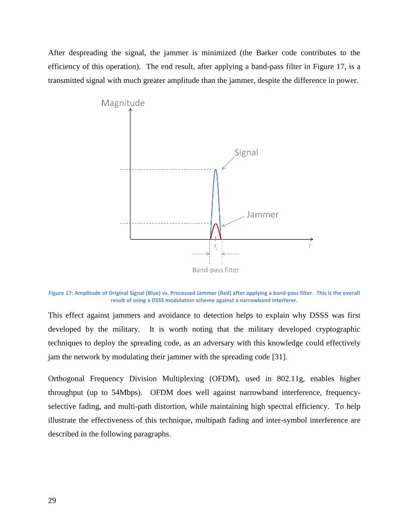
29

After despreading the signal, the jammer is minimized (the Barker code contributes to the

efficiency of this operation). The end result, after applying a band-pass filter in Figure 17, is a

transmitted signal with much greater amplitude than the jammer, despite the difference in power.

Figure 17: Amplitude of Original Signal (Blue) vs. Processed Jammer (Red) after applying a band-pass filter. This is the overall result of using a DSSS modulation scheme against a narrowband interferer.

This effect against jammers and avoidance to detection helps to explain why DSSS was first

developed by the military. It is worth noting that the military developed cryptographic

techniques to deploy the spreading code, as an adversary with this knowledge could effectively

jam the network by modulating their jammer with the spreading code [31].

Orthogonal Frequency Division Multiplexing (OFDM), used in 802.11g, enables higher

throughput (up to 54Mbps). OFDM does well against narrowband interference, frequency-

selective fading, and multi-path distortion, while maintaining high spectral efficiency. To help

illustrate the effectiveness of this technique, multipath fading and inter-symbol interference are

described in the following paragraphs.

30

Figure 18: Multipath signals bouncing off the environment. Signals suffer decay and arrive late at the receiver.

Multipath fading is common in any real-world application of wireless communication. The

original transmitted signal (Red) will follow multiple paths (Green and Blue), bounce off the

environment, and arrive at the receiver delayed in time and decayed in amplitude. Figure 19

shows the transmission of two signals at the transmitter (A), the ideal received signal (exactly the

same as the transmitted signal, B), and the realistic scenario of multiple signals arriving at the

receiver due to inter-symbol interference (C).

31

Figure 19: Transmitted Signal (A) with two symbols, Ideal Received Signal (B), Realistic Received Signal (C) with multiple, decayed, overlapping received symbols from ISI.

In Figure 19 (C), the delayed received signal of the first bit (Green) overlaps into the second bit

(Red), an effect called inter-symbol interference (ISI). If the two signals were spaced far enough

apart, their multipath equivalents would not affect the following signal. This problem worsens

when attempting high data-rate transmissions, as in Figure 20.

Figure 20: Transmitted signal with high bit-rate transmission (low symbol duration) (Left). Received signal with increased ISI (Right).

32

In order to squeeze more data into a shorter amount of time, the duration between each symbol is

shortened. This “shortening” causes the effects of inter-symbol interference to intensify, as the

travel time of multipath signals does not change with data-rate.

OFDM addresses this issue in a few ways; dividing carriers into sub-carriers with lower data

rates, using guard intervals between bands and symbols, and the addition of cyclic prefixes.

Figure 21 demonstrates the use of multiple carriers to send data.

OFDM encodes data with low rates on multiple carrier frequencies. This process diminishes

intersymbol interference (ISI). For example, when increasing the data rate, digital signals are

modulated with shorter durations. This makes them more susceptible to noise or other

impairments. However, dividing these carriers into subcarriers allows a high overall data rate

while maintaining a low data rate per carrier.

Figure 21: Using multiple carriers to send data (FDM). Advantages: Increased data rate and resistance to ISI using guard bands. Disadvantages: inefficient use of bandwidth.

By dividing one channel into many, each individual channel can use a lower data rate, but will

sum to the original, high-speed data rate. The lower data rates imply longer durations between

symbols and help to diminish ISI. However, this model, also known as Frequency Division

Multiplexing (FDM) is not bandwidth efficient. The introduction of orthogonal frequencies

allows a more efficient use of bandwidth.

33

Figure 22: Using overlapping carriers to send data (OFDM). Advantages: greatly increased data rate, resistance to ISI using guard bands, and efficient use of bandwidth. Disadvantages: sensitive to carrier frequency offset or drift.

Figure 22 demonstrates efficient use of bandwidth using OFDM sub-carriers for each channel.

IEEE 802.11a/g uses 52 sub-carriers (48 for data, 4 for pilot tones) [26]. This feature can be

explained by first examining the Fourier transform of a simple square signal in time, shown in

Figure 23.

Figure 23: Fourier transform of square, time domain signal into Sinc pulse in frequency domain. The bandwidth is inversely related to the spacing .

A square signal in time is a

function in frequency. Sinc pulses will intersect at

equally spaced points if they are spaced apart by . When utilizing this feature, each sub-

carrier is spaced such that, when sampled, it has no interference from the other frequencies.

Figure 24 illustrates this orthogonality with multiple overlapping sinusoids.

34

Figure 24: N=5 Overlapping OFDM tones. Each tone is orthogonal if the spacing between frequencies is equal to 1/NT. Note: minimal interference at sampling points (multiples of the symbol rate).

The symbol duration is inversely related to the spacing ; in other words, increasing the

data rate (shortening ) requires an increase in carrier spacing. Hence, a trade-off exists

between data rate and spectral efficiency (higher data rates require increased carrier spacing,

consuming more bandwidth).

These methods increase spectral efficiency, but inter-symbol interference is still an issue. To

reiterate the problem, consider Figure 25; it starts with the transmission of two symbols using

DBPSK (Blue), with a faded multipath symbol (Red) indicating inter-symbol interference (gray).

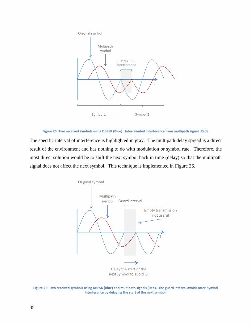
35

Figure 25: Two received symbols using DBPSK (Blue). Inter-Symbol Interference from multipath signal (Red).

The specific interval of interference is highlighted in gray. The multipath delay spread is a direct

result of the environment and has nothing to do with modulation or symbol rate. Therefore, the

most direct solution would be to shift the next symbol back in time (delay) so that the multipath

signal does not affect the next symbol. This technique is implemented in Figure 26.

Figure 26: Two received symbols using DBPSK (Blue) and multipath signals (Red). The guard interval avoids Inter-Symbol Interference by delaying the start of the next symbol.

36

Notice that the next symbol does not start until the end of the multipath symbol, thus ISI has

been eliminated. However, an empty transmission in time is not technically applicable in most

hardware (which outputs continuous signals) and could cause disruptions and desynchronization

in the receiver. A solution to this problem is to fill the guard interval with the tail of the symbol,

depicted in Figure 27.

Figure 27: Two received symbols using DBPSK (Solid Blue) with a Cyclic Prefix (Dashed Blue) added to avoid ISI. The cyclic extension is taken from the tail end of the symbol and added to the front.

This technique eliminates ISI by including a tail of the symbol to fill the guard interval, and

allows the beginning of symbols to become corrupted without affecting demodulation. Figure 28

shows an alternative view of the transmitted symbol using cyclic extensions.

Figure 28: Alternate view of the transmitted signal using Cyclic Prefix. The received signal avoids ISI.

37

OFDM will typically use 0.8 µS for the cyclic prefix, based on the maximum delay spread of the

environment, and not necessarily to every sub-carrier [26]. The one drawback with this method

is the loss in data rate used to include the redundant information (the cyclic prefix). OFDM is

also implemented in the latest 802.11n standard with Multiple Input Multiple Output (MIMO),

achieving longer range and increased data rates (up to 600 Mbps) via multiple antennas [32].

MAC Layer

Nearly every form of wireless communication includes a MAC layer or protocol (Medium

Access Control). In wireless communication, only one person can talk at a time on the same

channel. The MAC Layer defines the rules on how clients share the channel equally while

minimizing interference, in addition to accounting for reliable delivery and security. In the most

basic sense, the MAC layer is the protocol that dictates who gets to use the “talking stick,” and

when. In Wi-Fi, this is implemented in two main fashions: a Distributed Coordinate Function

(DCF), and a Point Coordinate Function (PCF, implemented on top of the DCF). PCF is used in

Access Point (AP) mode, where there exists a server or “leader” who takes control and organizes

the network. DCF is used in Ad-hoc mode, where there is no formal structure or leader and all

users rely on a protocol of how to share the medium with each other. A four node example of

the two basic network configurations is shown in Figure 29.

Figure 29: Differences between Access Point (Central Server or Point Coordination) and Ad-hoc Networks (Mesh or Distributed Coordination).

38

In each scenario in Figure 29, one node wishes to transmit (bottom left node). In AP networks,

the point coordinator (PCF) issues the NAV signal to all other nodes, allowing the one client to

transmit. The AP will also issue contention-free periods (NAV signals) to stop all other

terminals and poll other stations in a semi-periodic fashion [28]. Ad-hoc networks rely on a set

of rules to allow each user a fair chance at using the medium, and decide when to transmit and

when to be silent based on those rules.

At the heart of the DCF is a protocol called Carrier Sense Multiple Access (CSMA). This is

simply a process by which the channel is sensed (virtually and physically) before attempting to

transmit. A critical component of CSMA is a priority schema, where three different Inter-frame

Spacings (IFS), described in Table 3, exist for different types of packets,

Table 3: Definitions of Inter-frame Spacings and their role in the MAC Layer [14].

Name Definition

IFS Inter-frame Spacing. The amount of time to wait to transmit after the medium has been

sensed as busy.

SIFS Short IFS. The shortest duration (highest priority) to wait to transmit. This is used in

Acknowledgement (ACK), Clear to Send (CTS), and Poll Response messages.

PIFS Point Coordination Function IFS. This is used in Access Point mode by the central

controller when issuing polls or to take precedence over DIFS.

DIFS Distributed Coordinate Function IFS. The longest duration (lowest priority), used for all

ordinary traffic.

The IFS between transmissions allow specific packets to have priority over others. The SIFS

primarily allows some room for receivers to respond before others begin transmitting, such as

when a receiver sends an ACK to confirm delivery to the transmitter, or when a receiver signals

others that a transmission is about to begin (CTS). The PIFS is used by an Access Point or

“point coordinator” to maintain priority control of the channel. All other traffic must wait the

duration of DIFS before attempting to transmit. Figure 30 demonstrates the use of IFS and a

backoff window, explained in the following paragraph.

39

Figure 30: IEEE 802.11 MAC Access Method using Inter-frame Spacings and the Exponential Backoff Algorithm [14, p. 530].

If one or more radios transmit while the medium is busy, a collision can occur. To reduce the

probability of collisions and provide equal opportunity for transmission, each radio uses an

exponential backoff algorithm. The algorithm attempts to space out repeated transmissions in a

populated network [28]. This involves choosing a random number, and while the medium is

free, waiting that number of time slots before attempting to transmit. If the medium is sensed as

busy, the timer freezes until the channel is idle again. Further collisions cause the timer to

increase exponentially.

As shown in Figure 30, after waiting DIFS, any client is allowed to transmit if the medium is

free. Once transmission is detected, all clients activate their Network Allocation Vector (NAV,

an indicator of a busy channel) signal for the duration of the transmission. The receiving client

will wait the duration of SIFS and return an ACK, CTS or Poll Response message, if necessary.

If an Access Points needs to take control of the medium after transmission, it will wait the

duration of PIFS. Other clients will wait the duration of DIFS before attempting to transmit. At

this point, if one client is unable to gain access to the medium or notices a collision with another

client, it will begin counting its backoff timer while the medium is idle, then when the timer

reaches zero it will attempt to retransmit. A general overview of this process is shown in Figure

31.

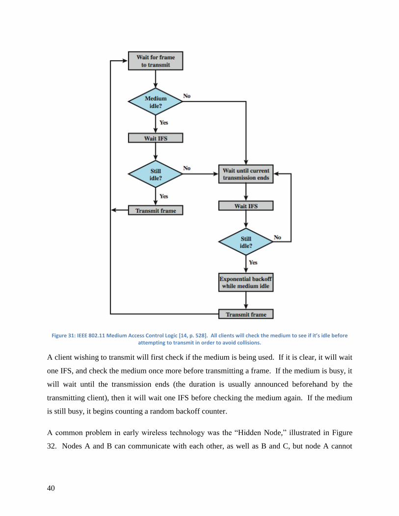
40

Figure 31: IEEE 802.11 Medium Access Control Logic [14, p. 528]. All clients will check the medium to see if it’s idle before attempting to transmit in order to avoid collisions.

A client wishing to transmit will first check if the medium is being used. If it is clear, it will wait

one IFS, and check the medium once more before transmitting a frame. If the medium is busy, it

will wait until the transmission ends (the duration is usually announced beforehand by the

transmitting client), then it will wait one IFS before checking the medium again. If the medium

is still busy, it begins counting a random backoff counter.

A common problem in early wireless technology was the “Hidden Node,” illustrated in Figure

32. Nodes A and B can communicate with each other, as well as B and C, but node A cannot

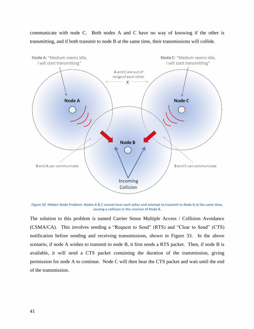
41

communicate with node C. Both nodes A and C have no way of knowing if the other is

transmitting, and if both transmit to node B at the same time, their transmissions will collide.

Figure 32: Hidden Node Problem: Nodes A & C cannot hear each other and attempt to transmit to Node B at the same time, causing a collision in the receiver of Node B.

The solution to this problem is named Carrier Sense Multiple Access / Collision Avoidance

(CSMA/CA). This involves sending a “Request to Send” (RTS) and “Clear to Send” (CTS)

notification before sending and receiving transmissions, shown in Figure 33. In the above

scenario, if node A wishes to transmit to node B, it first sends a RTS packet. Then, if node B is

available, it will send a CTS packet containing the duration of the transmission, giving

permission for node A to continue. Node C will then hear the CTS packet and wait until the end

of the transmission.

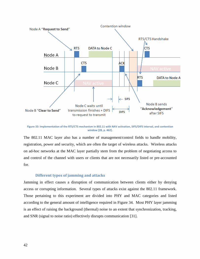
42

Figure 33: Implementation of the RTS/CTS mechanism in 802.11 with NAV activation, SIFS/DIFS interval, and contention window [28, p. 462].

The 802.11 MAC layer also has a number of management/control fields to handle mobility,

registration, power and security, which are often the target of wireless attacks. Wireless attacks

on ad-hoc networks at the MAC layer partially stem from the problem of negotiating access to

and control of the channel with users or clients that are not necessarily listed or pre-accounted

for.

Different types of jamming and attacks

Jamming in effect causes a disruption of communication between clients either by denying

access or corrupting information. Several types of attacks exist against the 802.11 framework.

Those pertaining to this experiment are divided into PHY and MAC categories and listed

according to the general amount of intelligence required in Figure 34. Most PHY layer jamming

is an effect of raising the background (thermal) noise to an extent that synchronization, tracking,

and SNR (signal to noise ratio) effectively disrupts communication [31].

43

Figure 34: Jamming Attacks at MAC & PHY Layer. Techniques are listed by intelligence required.

A short list of PHY layer attacks in Table 4 consist of RF Jamming using noise (typically

Additive White Gaussian Noise [AWGN]) in sweeping patterns, random bursts or pulses, or

even modulated data using Differential Binary Phase Shift Keying (DBPSK) or other

modulations. Modulated (deceptive) noise works to fool a receiver into thinking the signal is

important or contains information, often forcing it to spend time and energy decoding the signal.

MAC layer attacks, listed in Table 5, are more complex and require some knowledge of the

network. Jamming methods at higher layers (MAC and above) typically require intelligence

gathering before commencing an attack.

Table 4: PHY Layer Jamming Definitions.

Name Definition

Constant Continuous jamming with AWGN.

Sweep Continually jamming, typically with a single carrier tone, in a sweep pattern

across a range of frequencies.

Deceptive Modulating noise to appear as though it contains information.

Random/Pulse Transmitting signals at random intervals to save power and avoid detection.

Reactive/Corruption Jamming for short durations to destroy packets when a transmission is detected.

44

Each technique in Table 4 has its own advantages and disadvantages. For example, constant

jamming requires the most power, but will completely prevent communication in the target area,

especially when using directed antennas. Soldiers have been known to use constant jammers

with omni-directional antennas to prevent radio-activated I.E.D.’s (Improvised Explosive

Devices) from being triggered by remote, but in most cases they will not be able to use radios

themselves [33]. Most PHY layer attacks do not discriminate between friends and foes, but

MAC layer attacks have the potential to selectively target clients. A short list of attacks relative

to this report is defined in Table 5.

Table 5: MAC Layer Jamming Definitions.

Name Definition

Deauthentication/Disassociation Spoof (fake) frames that force clients to disconnect from each other.

Backoff Manipulation Fooling a receiver to increase the time spent waiting to avoid

collisions.

NAV Spoofing Cause other clients to wait until the channel is busy by sending fake

CTS/RTS messages.

Channel Switch Fooling or causing a transmitter to switch channels unnecessarily.

De-synchronization Altering time stamps in management frames in order to cause de-

synchronization at the receiver.

Flooding Sending many (thousands or more) of beacons or association requests

in order to overflow the association table.

Reactive Frame Injection Injecting malicious information into management frames on rate,

encryption, channel, and association, immediately after the target’s

frame.

Unlike PHY layer jamming, the effectiveness and efficiency of MAC attacks vary depending on

the protocol used by the target. The techniques in Table 5 are specific to 802.11b/g, but can

occasionally be applied to other existing protocols, which is why some ‘intelligence gathering’ is

45

necessary with higher layer attacks. One of the most effective techniques is a deauthentication or

disassociation attack, which constantly spoofs frames that disconnect you from other nodes,

making communication near impossible. However, effectiveness does not always imply

efficiency, an important parameter in ad-hoc networks, as they are usually mobile and rely on

battery power. A chart which categorizes several of the above listed attacks is shown in Figure

35. Note that this chart is subjective generalized; any PHY jammer can be made 100% effective

with enough power, and any MAC layer attack can prove more effective depending on the

protocol and hardware used in the network.

Figure 35: Chart of Effectiveness vs. Efficiency of PHY (RED) and MAC (BLUE) layer attacks. Note: All attacks are subjective.

PHY layer attacks are inherently more effective, as they prevent the most basic use of a medium,

but are typically less efficient. Constant jamming is the least efficient as it consumes the most

power and involves unceasing transmission. An exception is reactive jamming, which involves

transmitting a small burst of noise when an on-going transmission has been detected, and is

considered one of the most efficient methods of RF jamming. Unlike some naïve PHY jamming

techniques which are not very efficient (constant, sweep, random, pulse), MAC attacks have the

potential to substantially decrease effective throughput using far less energy.

46

NAV spoofing is slightly less efficient and effective since it has to repeatedly spoof CTS/RTS

frames, and cannot destroy other packets. We propose that the reactive frame injection method

will be of the same efficiency of NAV spoofing, since it will transmit with similar periodicity.

However, reactive frame injection could prove more effective than NAV spoofing, since it has

the power to selectively silence communications, whereas NAV spoofing can only silence all

clients in the area except one node.

47

3 Methods

As previously discussed, this project is composed of two distinct, but closely related, parts:

testbed construction and a Wi-Fi denial of service attack on that testbed. Both components are

equally important and dependent on each other. The testbed provides a mechanism to test the

team’s proposed MAC layer Wi-Fi attack while the well known PHY layer jamming attacks

provide the team with a way to validate the testbed. In this chapter, the team will explain the

process of developing, executing, and testing/validating the different key components of this

project. This will include a description of the testbed design process and the techniques use to

perform preliminary testing. The team will also cover the techniques used to perform PHY layer

jamming, starting off the testbed to create a point of comparison and then moving to the testbed

to confirm testbed functionality. Lastly, the team will discuss the development and execution of

the MAC layer attack performed on the testbed.

3.1 Testbed design process

Before settling on a final design for the testbed, the team explored some preliminary ideas. Ideas

were based upon the original specifications provided to the team by mentors at MIT Lincoln

Laboratory. These specifications included:

Wideband (30 MHz – 7 GHz)

Support for 6 radio nodes

Isolation no less than 20 dB between fingers of splitters

No more than 45 dB of loss throughout the system

No more than 2 dB of variation in loss between the different paths through the system

Attenuators switch within 1ms timing

Although the original design ideas were not ultimately the chosen solutions, they played an

important role in the design process. Evaluating the pros and cons of these initial designs led the

team to the final testbed design that best met specifications.

48

Original Design Ideas and Assessment

Prior to commencing any detailed design, the team constructed a very basic outline of the testbed

and its key components. Figure 36 below is a visual summary of the basic channel emulator

structure with its most fundamental components.

Figure 36: Basic structure of analog channel emulator with key parts (A) Circulator (B) Power Splitter/Combiner and (C) Programmable Attenuator. This diagram shows a channel emulator that supports only three radio nodes.

This design schematic is a scaled down channel emulator that supports three radios, although the

same concepts in this design can be scaled up to support more nodes. In the schematic, each of

the three radios is connected up to a circulator, Figure 36 (a), which allows the radio to transmit

and receive simultaneously. The transmit path connects to a power splitter, Figure 36 (b), which

divides the power from each radio three ways. Two of the three RF paths created by the splitter

49

connect to a programmable attenuator, Figure 36 (c), which allows the user to control the

magnitude of the signal sent from each radio to all of the other radios. The remaining RF path,

which does not connect to an attenuator, can either be terminated with a 50Ω load or can be sent

to an oscilloscope or spectrum analyzer.

A second set of three-way splitters recombine signal power from two of the radios and send it

back to the receiving port of the circulator. In summary, the fundamental testbed design was

found to need three important key parts or functions: circulators to provide isolation between TX

and RX, splitters/combiners, and programmable attenuation.

With the important functions of the testbed determined, specific parts to perform these key

functions were selected. Because the specifications are for a six radio testbed, the splitters need

to be six-way, unlike in Figure 36, where the splitters were three-way to support a three radio

testbed. Considering the specifications, the team put together two different lists of parts for two

different design schemes. Both designs use a Hittite Microwave programmable attenuator

(HMC-C018) that works from DC to 13 GHz and provides attenuation from 0 to 31.5 dB in steps

of 0.5 dB.

When programmed to the 0 dB attenuation state, this attenuator has an insertion loss of 4 dB.

Both designs also involved a more narrowband circulator, on hand in the laboratory, which could

be switched out for a more permanent wideband solution later on. The design ideas differed in

their implementation of the six-way splitter.

The first design scheme creates the six way splitters out of one two-way resistive power splitter

(Mini-Circuits ZFRSC-123+) cascaded with two three way splitters (Mini-Circuits SF3RSC-

542+). A diagram of the composite six-way splitter is shown below in Figure 37.

50

Figure 37: Six-way splitter composed of cascaded two and three-way splitters. This design was not ultimately used because it was too lossy.

Isolation between the fingers of the different splitters, as described on the data sheet, is shown in

Figure 37. The two-way splitter has an isolation of 18 dB between fingers of the splitter while

the three way splitter has isolation of 19.5 dB. While the isolation in this splitter is relatively

close to the specifications, it is extremely lossy, with 10 dB in each two-way splitter and 20dB in

each three way splitter. When a radio transmits, the power goes through the circulator, the

cascaded splitters, back through a different set of cascaded splitters, and finally back through the

circulator again. The total loss due to travelling through the six way splitters alone is 60 dB.

This is far above the given 45 dB specification for loss throughout the system. In addition, the 6

way splitter only supports a bandwidth of DC - 5.4 GHz which falls short of the bandwidth

specification.

51

The second design idea involved cascading five two-way power splitters (Mini-Circuits ZX10R-

14+) to create the six way splitter/combiner. These splitters have less loss, specifically 7.5 dB

per two-way splitter and 45 dB total for the two six-way splitters created by cascading them, but

this is still too much.

Figure 38: Five two-way splitters cascaded to create a six-way splitter. This design was not ultimately used because it did not provide enough isolation.

While the second design idea supports the full specified band, the two way splitters only have 6

dB of isolation between the fingers of the splitters, as shown in Figure 38. This is substantially

lower than the specified isolation. The limitations of these two original design ideas are

summarized in

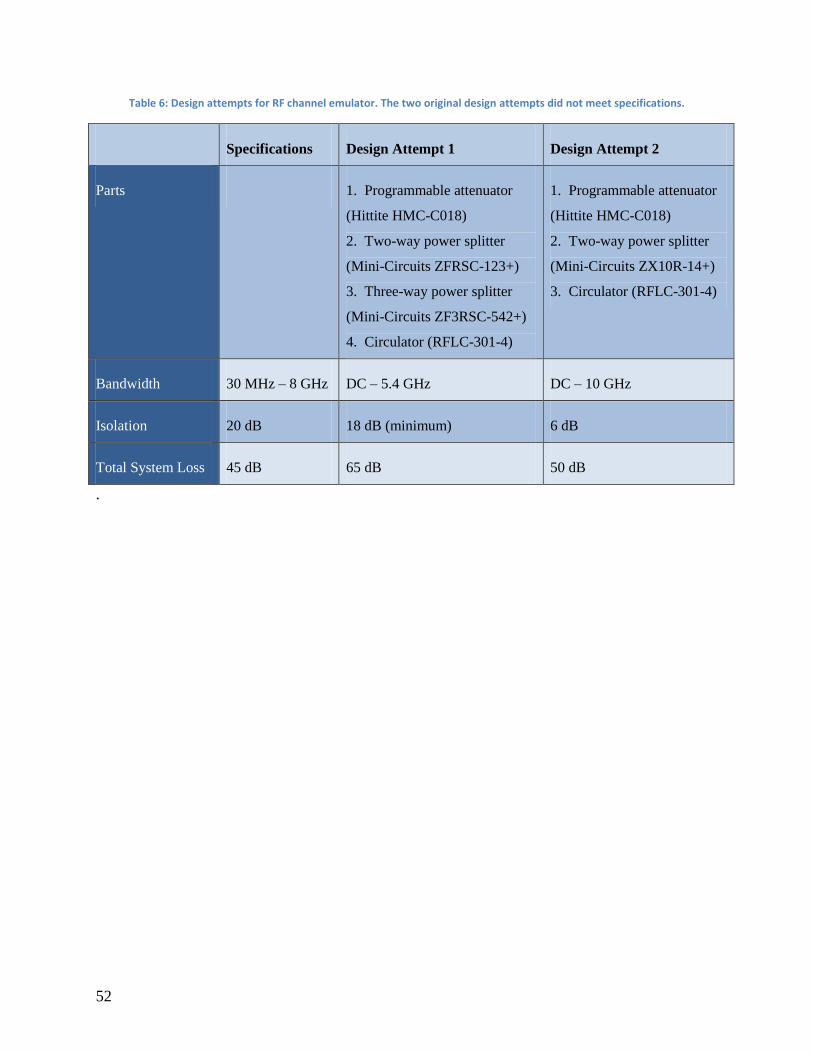
52

Table 6: Design attempts for RF channel emulator. The two original design attempts did not meet specifications.

Specifications Design Attempt 1 Design Attempt 2

Parts 1. Programmable attenuator

(Hittite HMC-C018)

2. Two-way power splitter

(Mini-Circuits ZFRSC-123+)

3. Three-way power splitter

(Mini-Circuits ZF3RSC-542+)

4. Circulator (RFLC-301-4)

1. Programmable attenuator

(Hittite HMC-C018)


(Mini-Circuits ZX10R-14+)


Bandwidth 30 MHz – 8 GHz DC – 5.4 GHz DC – 10 GHz

Isolation 20 dB 18 dB (minimum) 6 dB

Total System Loss 45 dB 65 dB 50 dB

.

53

Table 6: Design attempts for RF channel emulator. The two original design attempts did not meet specifications.

Specifications Design Attempt 1 Design Attempt 2

Parts 1. Programmable attenuator

(Hittite HMC-C018)


(Mini-Circuits ZFRSC-123+)

3. Three-way power splitter

(Mini-Circuits ZF3RSC-542+)


1. Programmable attenuator

(Hittite HMC-C018)


(Mini-Circuits ZX10R-14+)


Bandwidth 30 MHz – 8 GHz DC – 5.4 GHz DC – 10 GHz

Isolation 20 dB 18 dB (minimum) 6 dB

Total System Loss 45 dB 65 dB 50 dB

In summary, the original ideas both failed to meet specifications. The first design attempt had

almost enough isolation but too much loss and did not cover the desired bandwidth. The second

design attempt contained less loss than the first plan but still too much, and, while it covered the

full band, it had far too little isolation. Learning from these first passes at the problem helped the

team produce the final design.

Final Design

Due to the difficulty meeting the system specifications for such a wide bandwidth, the team

decided to employ band breaks in the system. Distinct sets of parts are used to support the lower

and upper portions of the frequency band. Based upon a review of available parts, the team

decided to have the lower frequency band support 30 MHz to 3 GHz and the higher frequency

band support 2 to 8 GHz, with an overlap from 2 to 3 GHz. Diplexers could be used to direct

signal of different frequency content through the two different channels of the testbed. Due to

the early difficulties finding resistive power dividers that could provide the desired isolation and

frequency coverage without too much loss, the team decided to use cascaded directional couplers

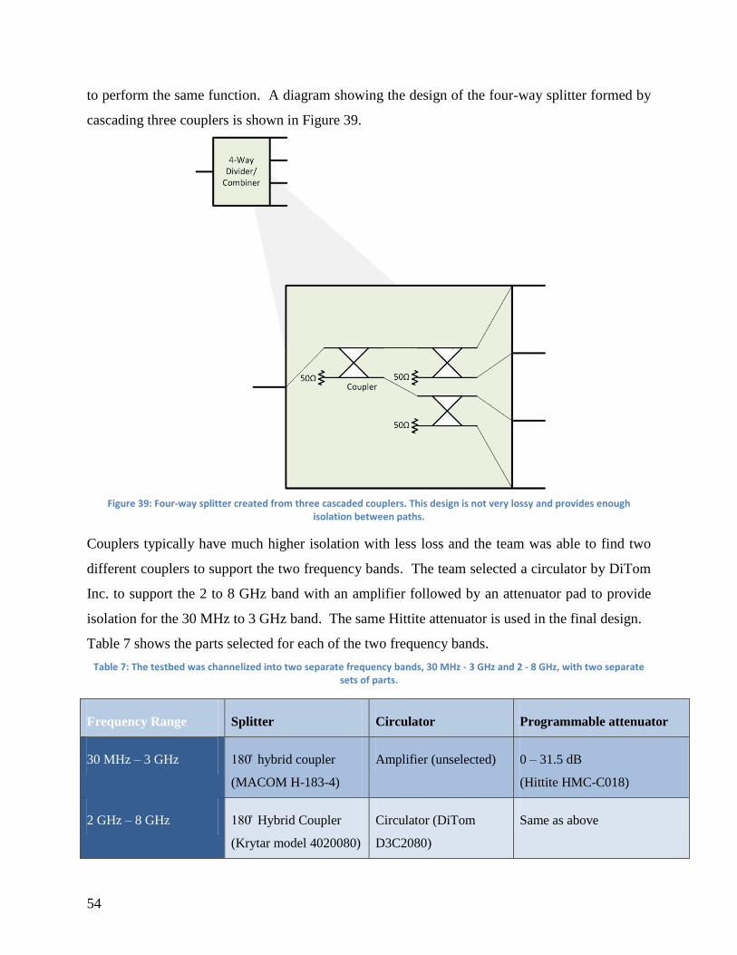
54

to perform the same function. A diagram showing the design of the four-way splitter formed by

cascading three couplers is shown in Figure 39.

Figure 39: Four-way splitter created from three cascaded couplers. This design is not very lossy and provides enough isolation between paths.

Couplers typically have much higher isolation with less loss and the team was able to find two

different couplers to support the two frequency bands. The team selected a circulator by DiTom

Inc. to support the 2 to 8 GHz band with an amplifier followed by an attenuator pad to provide

isolation for the 30 MHz to 3 GHz band. The same Hittite attenuator is used in the final design.

Table 7 shows the parts selected for each of the two frequency bands.

Table 7: The testbed was channelized into two separate frequency bands, 30 MHz - 3 GHz and 2 - 8 GHz, with two separate sets of parts.

Frequency Range Splitter Circulator Programmable attenuator

30 MHz – 3 GHz 180 hybrid coupler

(MACOM H-183-4)

Amplifier (unselected) 0 – 31.5 dB

(Hittite HMC-C018)

2 GHz – 8 GHz 180 Hybrid Coupler

(Krytar model 4020080)

Circulator (DiTom

D3C2080)

Same as above

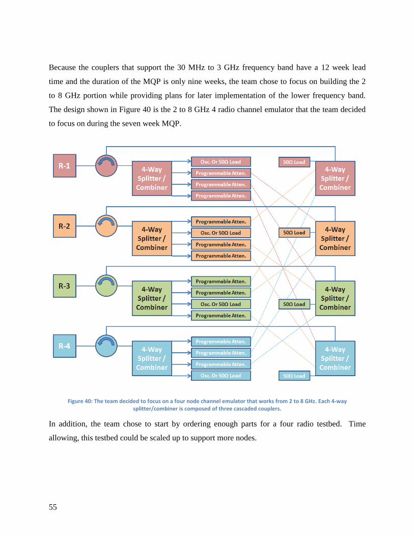
55

Because the couplers that support the 30 MHz to 3 GHz frequency band have a 12 week lead

time and the duration of the MQP is only nine weeks, the team chose to focus on building the 2

to 8 GHz portion while providing plans for later implementation of the lower frequency band.

The design shown in Figure 40 is the 2 to 8 GHz 4 radio channel emulator that the team decided

to focus on during the seven week MQP.

Figure 40: The team decided to focus on a four node channel emulator that works from 2 to 8 GHz. Each 4-way splitter/combiner is composed of three cascaded couplers.

In addition, the team chose to start by ordering enough parts for a four radio testbed. Time

allowing, this testbed could be scaled up to support more nodes.

56

3.2 Attenuator Control

Controlling attenuators in the testbed in order to simulate changing radio geometries was an

important aspect of the testbed design. Design specifications call for attenuators to be able to

switch, as a group, within a millisecond or less. The chosen attenuator, Hittite’s HMC-C018, is

capable of switching at this speed or faster. This specific attenuator has four digital inputs

(clock, reset, serial input, and latch) and requires a negative five volt power rail and ground. Due

to availability, a National Instruments PCI card (NI 6601) with digital I/O was selected to serve

as the control interface. Digital signals from the card were routed through a National

Instruments SCB-68 breakout board and to a breadboard where the attenuators were connected.

Originally, the team planned to control the cards using MATLAB. During assembly and testing

of the attenuator control circuit, a number of problems arose and were addressed, ultimately

leading to the final design.

In order to simulate a moving configuration of radio nodes, radio separation is represented with

meaningful attenuation values. A MATLAB function was written to calculate attenuation values

between all node pairs at certain time intervals based upon the start location of each radio, the

stop location of each radio, and the duration of the experiment in seconds. The attenuation

values calculated by this function are converted to a bit pattern to be written to the PCI card.

Originally the team intended to use MATLAB to write digital words to the card but this method

was found to be too slow for the speed specification. To address the speed concern, the bit

pattern produced in MATLAB was written to a text file. A C program reads the text file line by

line and writes each line to the PCI card.

While the PCI card was able to write values to the attenuators at an adequate speed

(approximately 40 kHz), voltage overshoot on the different lines was found to be substantial.

The clock line had ringing as much as three volts above the five volt logic high and as much as 2

volts below zero on the falling edge. These values exceed maximum ratings for the data pins of

the attenuators. In order to address ringing, a ringing suppressant circuit was added at the end of

each data line on the bread board. This circuit is shown in Figure 41 below.

57

Figure 41: Original ringing suppressing circuit with PCI Card (Left) and Programmable Attenuator (Right). This circuit worked well enough when there were fewer attenuators.

When the data line goes high, the lower diode goes into reverse bias and the drop across the

upper diode goes to approximately zero. The diodes help to clamp down on overshoots in the

digital signal and the resister dampens the ringing even further. While this circuit slows the rise

and fall times, it did not appear to negatively impact the functionality of the attenuator.

Further challenges were encountered in scaling up the setup to support additional attenuators.

Initially, the design involved supporting multiple attenuators with a shared clock, latch, and reset

pin because these pins are the same for all of the attenuators. It is the serial input that determines

each attenuators unique value so every attenuator has a distinct serial line. However, a single

clock, latch, and reset pin were found to be insufficient to support more than two attenuators

reliably. This is most likely due to a considerable voltage drop across the large resister used to

dampen ringing. In response to this issue, more clock, reset, and latch lines were broken out

from the card such that each line supports no more than two attenuators. The additional clock

lines remedied the power issues but increased ringing in all of the other signal lines. Ringing in

many of the latch lines occurred whenever the clock switched states, sometimes causing the

attenuator to latch a new value. To resolve this problem, a new ringing suppressing circuit was

designed. This circuit is shown in Figure 42.

58

Figure 42: Final ringing suppressing circuit with added buffer capacitors placed within close proximity to data lines, and twisted pair cables (paired with GND) for each data signal. Note: Twisted Pair cable is not an inductor.

In addition to suppressing the ringing with the circuit shown in Figure 42, other precautions were

taken to ensure the integrity of the digital lines. All alike lines were grouped together to

minimize the exposure of lower frequency signals like the latch to ringing caused by higher

frequency signals like the clock. Also, each signal line was twisted with a ground from the

breakout board as suggested by the PCI card datasheet. These precautions in combination with

the new ringing suppressing circuit worked well and are part of the final design. Once the

system that drives the attenuators was completely designed, attenuators were added to the system

one by one and tested individually to ensure functionality. With the final design of the testbed

was determined, the team selected several techniques for testing individual parts and then the

testbed as a whole. These methods will be discussed in the subsequent section.

3.3 Testbed construction and preliminary testing

In order to verify the functionality of each individual component in the testbed as well as the

system as a whole, the team conducted a variety of tests. S-parameter measurements were

collected for individual parts and for the assembled system. Two-tone testing was used to

measure the linearity of attenuator and assembled testbed. Finally, the rise and fall time of the

59

attenuator transitioning between different attenuation states was measured. The techniques used

to perform these various tests will be described below.

An Agilent E8364C PNA Network Analyzer was used to measure the s-parameters of all of the

parts individually. In instances where many of the same part were used, with the exception of

the attenuators, several parts were randomly selected and measured to assess the degree of

variability across the parts. Measurements were saved as .s2p files and processed in MATLAB.

These s-parameter measurements were used to produce graphs showing the insertion loss of each

component across the 2 to 8 GHz frequency band. Attention was also paid to the isolation

between the -3 dB ports of the coupler and the accuracy and flatness of the different attenuator

states throughout the complete frequency range. In order to collect this data, each attenuation

state was programmed into the device and then s-parameter data was collected. In addition,

return loss (S11) was measured for all of the different components and then for the system as a

complete unit. System gain was also measured.

Additional tests were performed on the assembled system beyond just those performed using the

network analyzer, including a two tone test and a measurement of rise and fall time in the

attenuator. One of these tests was a two tone test to measure the third-order intercept point of the

device. This is a measurement to determine the degree of nonlinearity in a system. In a two-tone

test, two sinusoids of equal power, approximately a megahertz apart, are fed into a system. The

setup we used is shown below in Figure 43.

Figure 43: Two-tone test setup. From left to right: Signal Generators, Isolators, Power Divider, Device Under Test (DUT), Spectrum Analyzer. The two-tone test helps to identify third order nonlinearities of a RF device.

60

The circulators shown in the diagram, with the third port terminated in a fifty ohm load, are used

to increase isolation between the two branches of the power splitter. The splitter combines the

two sinusoids and feeds them into the device under test, the attenuator. The output of the

attenuator is fed to a spectrum analyzer which is used to measure the third-order intermodulation

products of the two sinusoids. Care was taken to ensure that the intermodulation products

originated in the attenuator rather than in the front end of the spectrum analyzer itself. If the first

fundamental tone is at frequency and the second tone is at frequency then the two third-

order intermodulation products are at:

(3.1)

(3.2)

If the test is set up properly, the third-order intermodulation products should be approximately

the same. In order to calculate the third-order intermodulation distortion , the power

measured at the third-order intermodulation products is subtracted from the power at one

of the fundamental tones [34]:

(3.3)

The output third-order intercept point is defined as

(3.4)

The input third-order intercept point is simply the output third-order intercept point

minus the gain G in the device.

(3.5)

The results of this test were used to confirm the values provided on the attenuator data sheet.

After testing each individual part and the testbed system as a whole, the team further validated

the testbed by executing a series of known PHY layer attacks using the testbed.

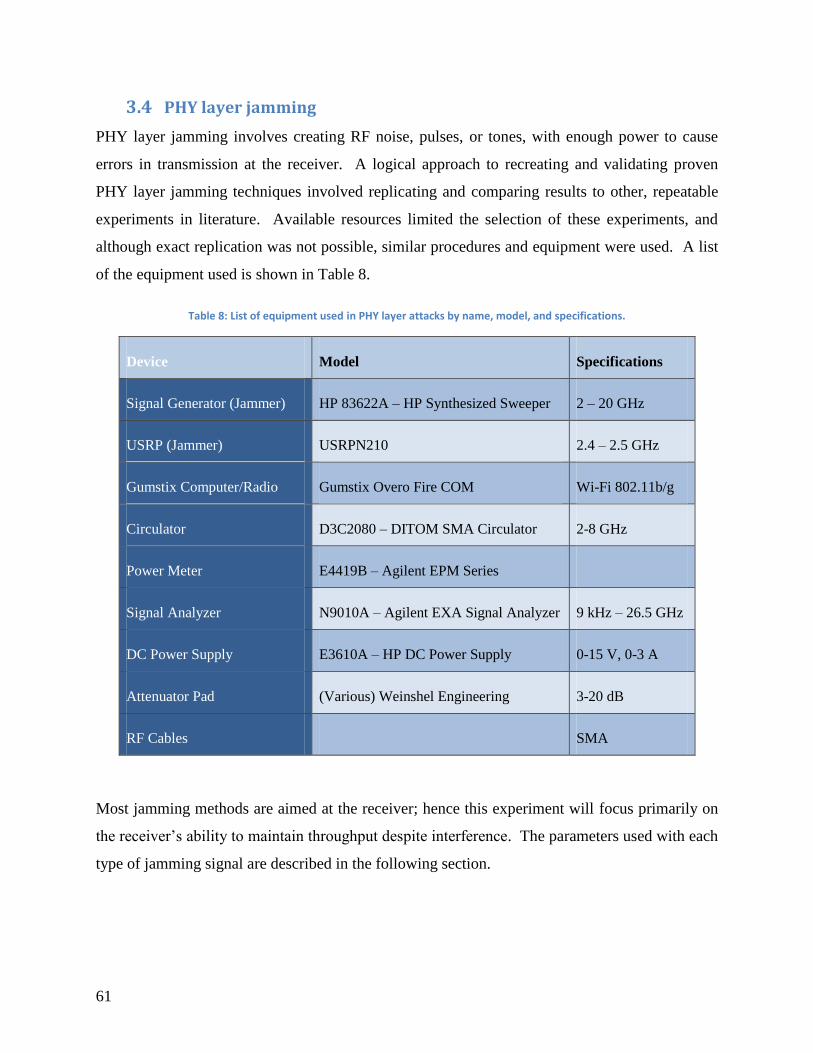
61

3.4 PHY layer jamming

PHY layer jamming involves creating RF noise, pulses, or tones, with enough power to cause

errors in transmission at the receiver. A logical approach to recreating and validating proven

PHY layer jamming techniques involved replicating and comparing results to other, repeatable

experiments in literature. Available resources limited the selection of these experiments, and

although exact replication was not possible, similar procedures and equipment were used. A list

of the equipment used is shown in Table 8.

Table 8: List of equipment used in PHY layer attacks by name, model, and specifications.

Device Model Specifications

Signal Generator (Jammer) HP 83622A – HP Synthesized Sweeper 2 – 20 GHz

USRP (Jammer) USRPN210 2.4 – 2.5 GHz

Gumstix Computer/Radio Gumstix Overo Fire COM Wi-Fi 802.11b/g

Circulator D3C2080 – DITOM SMA Circulator 2-8 GHz

Power Meter E4419B – Agilent EPM Series

Signal Analyzer N9010A – Agilent EXA Signal Analyzer 9 kHz – 26.5 GHz

DC Power Supply E3610A – HP DC Power Supply 0-15 V, 0-3 A

Attenuator Pad (Various) Weinshel Engineering 3-20 dB

RF Cables SMA

Most jamming methods are aimed at the receiver; hence this experiment will focus primarily on

the receiver’s ability to maintain throughput despite interference. The parameters used with each

type of jamming signal are described in the following section.

62

The signals listed below are created primarily with a USRP using GNURadio. Due to the

hardware limitations of the USRP (mainly, speed and bandwidth), a noise or signal generator

was used in creating large bandwidth signals and pulsed noise.

Digital Noise Jamming

o BPSK modulated pseudorandom data at 20 M samples/second using USRP &

GNURadio

Pulse Noise Jamming

o AWGN Noise pulsed with pulse lengths of 100 µS – 1000 µS and pulse intervals

of 1 mS to 10 mS.

Sweep Tone Jamming

o A single sine wave swept across the 2.4 GHz Wi-Fi band (100 MHz) in 0.5 to 20

seconds.

Validating the Testbed against Previous Experiments

Conducting experiments on a two-radio network allowed efficient use of time while waiting for

equipment to arrive (digital attenuators and couplers) while partially validating the procedure and

equipment against previous experiments in the literature[7], [35]. This also helped to prepare

and refine any methods used for the final experiment involving mobility, described in section

3.3.2. After all equipment had been prepared and assembled, our team implemented identical

tests on a three-radio (four nodes total) network before proceeding to mobile scenarios.

The two-radio network included two radio nodes, a jammer node, and a signal analyzer, shown

in Figure 44. The radio nodes consist of individual Gumstix computers, each with their own Wi-

Fi enabled 802.11b/g radio with external u.FL connectors (miniature coaxial RF connectors).

Special u.FL adapters were required to connect each radio to the SMA cables used in the

experiment. The jammer node was either a USRP or a signal generator depending on the

experiment. A signal analyzer measured the power level of the signal from the transmitter

compared to the signal from the jammer, also known as the Signal to Jammer Ratio (SJR).

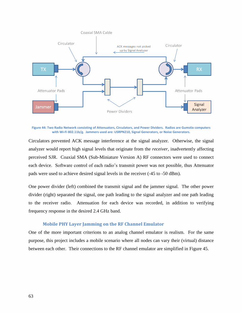
63

Figure 44: Two Radio Network consisting of Attenuators, Circulators, and Power Dividers. Radios are Gumstix computers with Wi-Fi 802.11b/g. Jammers used are: USRPN210, Signal Generators, or Noise Generators.

Circulators prevented ACK message interference at the signal analyzer. Otherwise, the signal

analyzer would report high signal levels that originate from the receiver, inadvertently affecting

perceived SJR. Coaxial SMA (Sub-Miniature Version A) RF connectors were used to connect

each device. Software control of each radio’s transmit power was not possible, thus Attenuator

pads were used to achieve desired signal levels in the receiver (-45 to -50 dBm).

One power divider (left) combined the transmit signal and the jammer signal. The other power

divider (right) separated the signal, one path leading to the signal analyzer and one path leading

to the receiver radio. Attenuation for each device was recorded, in addition to verifying

frequency response in the desired 2.4 GHz band.

Mobile PHY Layer Jamming on the RF Channel Emulator

One of the more important criterions to an analog channel emulator is realism. For the same

purpose, this project includes a mobile scenario where all nodes can vary their (virtual) distance

between each other. Their connections to the RF channel emulator are simplified in Figure 45.

64

Figure 45: Simplified diagram of connections between radio nodes and RF Channel Emulator. Each node can vary their distance between every other node.

The “RF Cloud” is a layer of abstraction controlled by digital attenuators that simulate distance,

allowing the experiment to demonstrate the effectiveness of a denial of service attack in a mobile

scenario. This layer of mobility allows the testbed to take one step closer to real-life. There are

a number of interesting mobile scenarios that are useful demonstrations of how well the DoS

attack would work, although only three are chosen for this report.

Listed in the following section are three mobile scenarios where the jammer is moving towards

or away from the network. In each experiment, the jammer node moves toward the network at a

rate of approximately 2 meters/second, passes within 3 meters of the closest radio node, and

continues through towards the end point. Iperf is used to exchange traffic at 11 Mbit/s using

802.11b (DSSS).

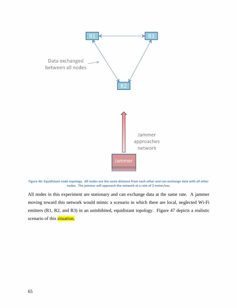
65

Figure 46: Equidistant node topology. All nodes are the same distance from each other and can exchange data with all other nodes. The jammer will approach the network at a rate of 2 meter/sec.

All nodes in this experiment are stationary and can exchange data at the same rate. A jammer

moving toward this network would mimic a scenario in which there are local, neglected Wi-Fi

emitters (R1, R2, and R3) in an uninhibited, equidistant topology. Figure 47 depicts a realistic

scenario of this situation.

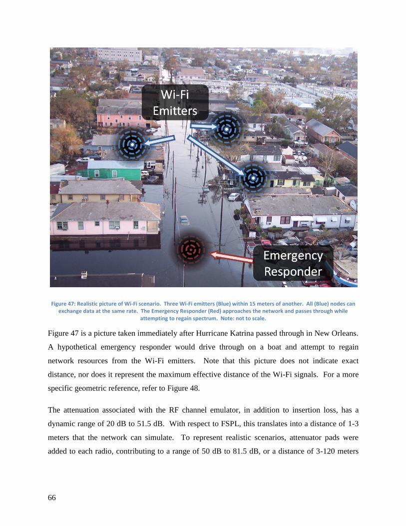
66

Figure 47: Realistic picture of Wi-Fi scenario. Three Wi-Fi emitters (Blue) within 15 meters of another. All (Blue) nodes can exchange data at the same rate. The Emergency Responder (Red) approaches the network and passes through while

attempting to regain spectrum. Note: not to scale.

Figure 47 is a picture taken immediately after Hurricane Katrina passed through in New Orleans.

A hypothetical emergency responder would drive through on a boat and attempt to regain

network resources from the Wi-Fi emitters. Note that this picture does not indicate exact

distance, nor does it represent the maximum effective distance of the Wi-Fi signals. For a more

specific geometric reference, refer to Figure 48.

The attenuation associated with the RF channel emulator, in addition to insertion loss, has a

dynamic range of 20 dB to 51.5 dB. With respect to FSPL, this translates into a distance of 1-3

meters that the network can simulate. To represent realistic scenarios, attenuator pads were

added to each radio, contributing to a range of 50 dB to 81.5 dB, or a distance of 3-120 meters

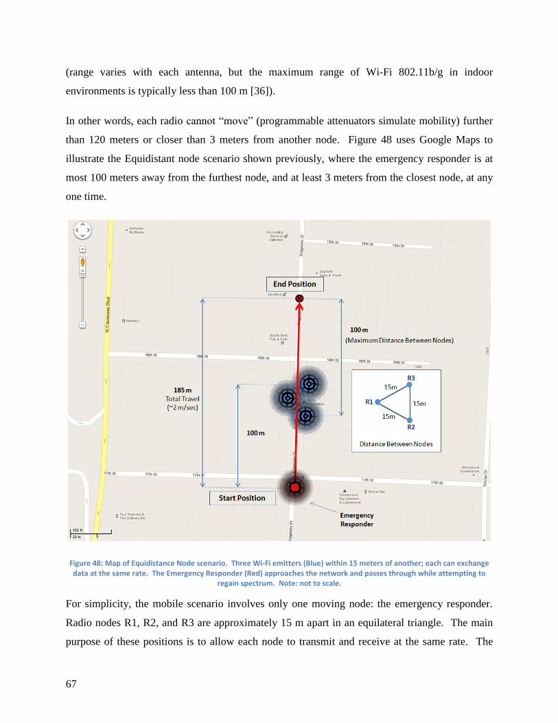
67

(range varies with each antenna, but the maximum range of Wi-Fi 802.11b/g in indoor

environments is typically less than 100 m [36]).

In other words, each radio cannot “move” (programmable attenuators simulate mobility) further

than 120 meters or closer than 3 meters from another node. Figure 48 uses Google Maps to

illustrate the Equidistant node scenario shown previously, where the emergency responder is at

most 100 meters away from the furthest node, and at least 3 meters from the closest node, at any

one time.

Figure 48: Map of Equidistance Node scenario. Three Wi-Fi emitters (Blue) within 15 meters of another; each can exchange data at the same rate. The Emergency Responder (Red) approaches the network and passes through while attempting to

regain spectrum. Note: not to scale.

For simplicity, the mobile scenario involves only one moving node: the emergency responder.

Radio nodes R1, R2, and R3 are approximately 15 m apart in an equilateral triangle. The main

purpose of these positions is to allow each node to transmit and receive at the same rate. The

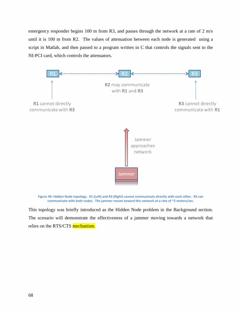
68

emergency responder begins 100 m from R3, and passes through the network at a rate of 2 m/s

until it is 100 m from R2. The values of attenuation between each node is generated using a

script in Matlab, and then passed to a program written in C that controls the signals sent to the

NI-PCI card, which controls the attenuators.

Figure 49: Hidden Node topology. R1 (Left) and R3 (Right) cannot communicate directly with each other. R2 can communicate with both nodes. The jammer moves toward this network at a rate of ~2 meters/sec.

This topology was briefly introduced as the Hidden Node problem in the Background section.

The scenario will demonstrate the effectiveness of a jammer moving towards a network that

relies on the RTS/CTS mechanism.

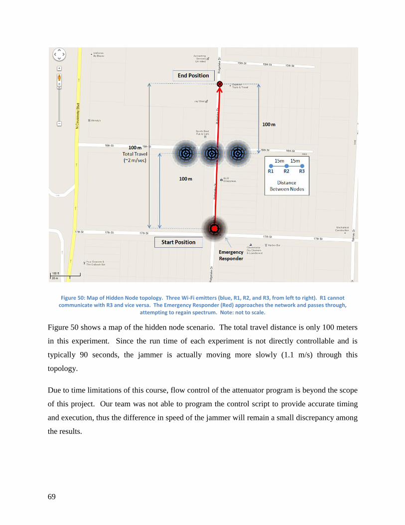
69

Figure 50: Map of Hidden Node topology. Three Wi-Fi emitters (blue, R1, R2, and R3, from left to right). R1 cannot communicate with R3 and vice versa. The Emergency Responder (Red) approaches the network and passes through,

attempting to regain spectrum. Note: not to scale.

Figure 50 shows a map of the hidden node scenario. The total travel distance is only 100 meters

in this experiment. Since the run time of each experiment is not directly controllable and is

typically 90 seconds, the jammer is actually moving more slowly (1.1 m/s) through this

topology.

Due to time limitations of this course, flow control of the attenuator program is beyond the scope

of this project. Our team was not able to program the control script to provide accurate timing

and execution, thus the difference in speed of the jammer will remain a small discrepancy among

the results.

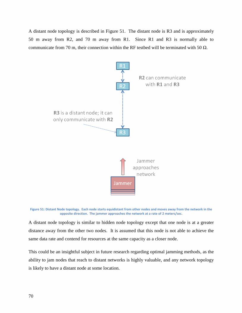
70

A distant node topology is described in Figure 51. The distant node is R3 and is approximately

50 m away from R2, and 70 m away from R1. Since R1 and R3 is normally able to

communicate from 70 m, their connection within the RF testbed will be terminated with 50 Ω.

Figure 51: Distant Node topology. Each node starts equidistant from other nodes and moves away from the network in the opposite direction. The jammer approaches the network at a rate of 2 meters/sec.

A distant node topology is similar to hidden node topology except that one node is at a greater

distance away from the other two nodes. It is assumed that this node is not able to achieve the

same data rate and contend for resources at the same capacity as a closer node.

This could be an insightful subject in future research regarding optimal jamming methods, as the

ability to jam nodes that reach to distant networks is highly valuable, and any network topology

is likely to have a distant node at some location.

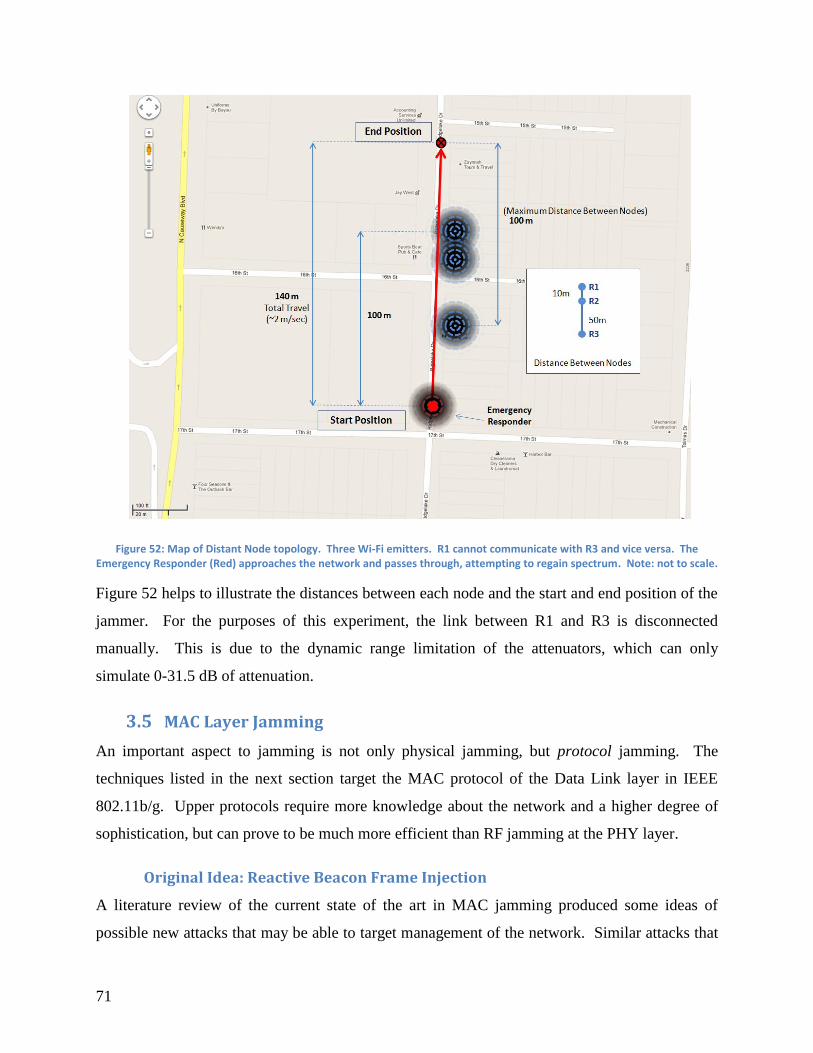
71

Figure 52: Map of Distant Node topology. Three Wi-Fi emitters. R1 cannot communicate with R3 and vice versa. The Emergency Responder (Red) approaches the network and passes through, attempting to regain spectrum. Note: not to scale.

Figure 52 helps to illustrate the distances between each node and the start and end position of the

jammer. For the purposes of this experiment, the link between R1 and R3 is disconnected

manually. This is due to the dynamic range limitation of the attenuators, which can only

simulate 0-31.5 dB of attenuation.

3.5 MAC Layer Jamming

An important aspect to jamming is not only physical jamming, but protocol jamming. The

techniques listed in the next section target the MAC protocol of the Data Link layer in IEEE

802.11b/g. Upper protocols require more knowledge about the network and a higher degree of

sophistication, but can prove to be much more efficient than RF jamming at the PHY layer.

Original Idea: Reactive Beacon Frame Injection

A literature review of the current state of the art in MAC jamming produced some ideas of

possible new attacks that may be able to target management of the network. Similar attacks that

72

target management frames are Disassociation or Deauthentication attacks which attempt to spoof

(fake) frames that tell others a client has left the network, forcing the target to continuously

rejoin the network before being able to transmit. Flooding attacks are also related; they spoof

management frames (beacon or authentication/association frames), typically thousands at a time,

in order to cause the client to overflow a buffer and crash, fill its association table, or to waste its

resources by continuously connecting with fake clients.

We propose a method called “Reactive Beacon Frame Injection,” based on manipulating the

exchange of network parameters such as data rate, encryption, synchronization, modulation, and

channel specification. This attack spoofs frames directly after (or immediately before) the target

user sends its own beacon, notifying all clients that the user wishes to use incorrect network

parameters (low data rates, weak encryption or none at all, unspecified modulation schemes,

etc.). It is suspected that this technique will force other clients to disregard the original beacon

frame and use the spoofed (manipulated) frame instead. This would cause other clients to use

the manipulated network parameters when sending packets to the target, forcing the target to

drop those packets. Figure 53 shows this procedure in action.

Figure 53: Reactive Beacon Frame Injection attack on IEEE 802.11b/g. The attack injects a manipulated beacon frame that seems as though it came from the target client. Subsequent packets sent to that client are then using the wrong network

parameters, resulting in dropped packets and/or weakened security.

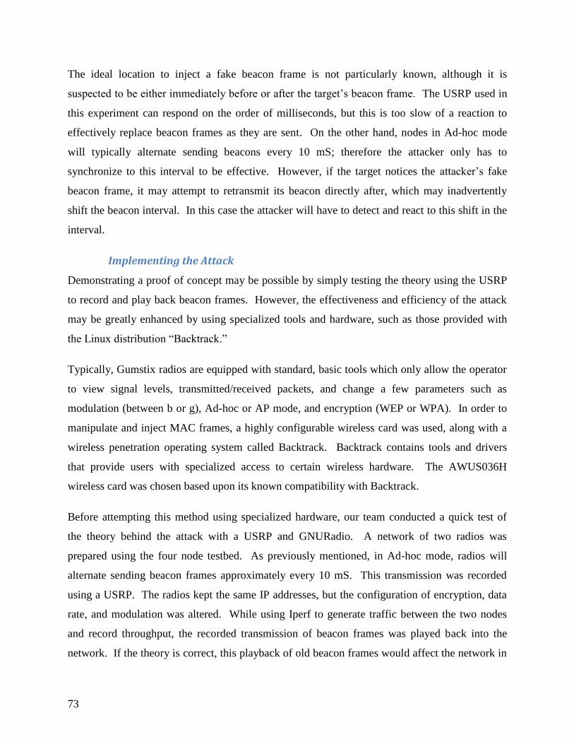
73

The ideal location to inject a fake beacon frame is not particularly known, although it is

suspected to be either immediately before or after the target’s beacon frame. The USRP used in

this experiment can respond on the order of milliseconds, but this is too slow of a reaction to

effectively replace beacon frames as they are sent. On the other hand, nodes in Ad-hoc mode

will typically alternate sending beacons every 10 mS; therefore the attacker only has to

synchronize to this interval to be effective. However, if the target notices the attacker’s fake

beacon frame, it may attempt to retransmit its beacon directly after, which may inadvertently

shift the beacon interval. In this case the attacker will have to detect and react to this shift in the

interval.

Implementing the Attack

Demonstrating a proof of concept may be possible by simply testing the theory using the USRP

to record and play back beacon frames. However, the effectiveness and efficiency of the attack

may be greatly enhanced by using specialized tools and hardware, such as those provided with

the Linux distribution “Backtrack.”

Typically, Gumstix radios are equipped with standard, basic tools which only allow the operator

to view signal levels, transmitted/received packets, and change a few parameters such as

modulation (between b or g), Ad-hoc or AP mode, and encryption (WEP or WPA). In order to

manipulate and inject MAC frames, a highly configurable wireless card was used, along with a

wireless penetration operating system called Backtrack. Backtrack contains tools and drivers

that provide users with specialized access to certain wireless hardware. The AWUS036H

wireless card was chosen based upon its known compatibility with Backtrack.

Before attempting this method using specialized hardware, our team conducted a quick test of

the theory behind the attack with a USRP and GNURadio. A network of two radios was

prepared using the four node testbed. As previously mentioned, in Ad-hoc mode, radios will

alternate sending beacon frames approximately every 10 mS. This transmission was recorded

using a USRP. The radios kept the same IP addresses, but the configuration of encryption, data

rate, and modulation was altered. While using Iperf to generate traffic between the two nodes

and record throughput, the recorded transmission of beacon frames was played back into the

network. If the theory is correct, this playback of old beacon frames would affect the network in

74

two ways: (1) the beacon frames may cause collisions in the transfer of packets, (2) the clients

will accept the recorded (false) beacon information and change their data rate, encryption and

modulation, and a subsequent drop in throughput should be observed.

A sophisticated attack could similarly be executed using tools found in Backtrack. The attack

begins with “Wireshark,” which captures beacon packets and uses the time stamps to specify the

beacon interval. The time-stamp, IP and MAC addresses are relayed to “aireplay,” a program

that can inject falsified beacon frames into the network. If successful, a script that can utilize

these programs will be able to implement the same beacon frame attack described above.

75

4 Results

Throughout the duration of the project, a variety of results and measurements were collected.

The team compiled several different types of data to verify the functionality of the testbed.

Before assembly, measurements were taken to characterize the performance of different testbed

components across the band. Once constructed, additional measurements were taken and known

PHY layer experiments were repeated on the testbed for validation and verification.

After the functionality of the testbed was characterized, three different types of PHY layer

jamming were implemented using the channel emulator mobility feature. Results from all of

these different measurements and experiments will be presented in the following chapter.

4.1 Channel Emulator: Testing and Validation

A number of different measurements were taken to validate and characterize the channel

emulator components and the system as a whole. S-parameters were collected for all of the

individual components as well as for the assembled testbed. Basic PHY layer jamming

techniques were performed using different RF hardware and then repeated on the testbed to

check performance. Channel emulator related results are below; starting with tests performed on

the individual components, followed by images of the assembled system and tests on the

complete emulator.

Hittite Attenuator

Results that describe the insertion loss and flatness of major attenuation states are shown below

in Figure 54. The measurement was taken on the network analyzer from DC to 8 GHz. Insertion

loss is shown in blue. Major attenuation states, including 0.5 dB, 1dB, 2 dB, 4 dB, 8 dB, and 16

dB, are shown in red. These states are adjusted to be relative to the insertion loss state of the

device.

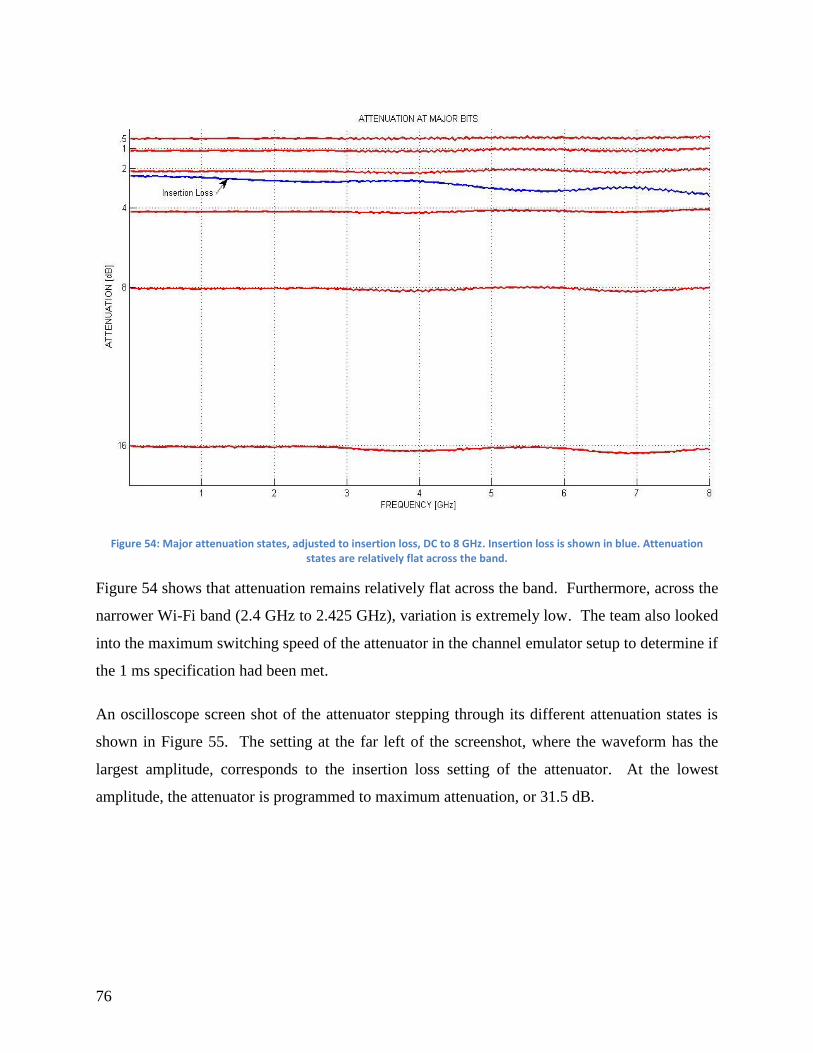
76

Figure 54: Major attenuation states, adjusted to insertion loss, DC to 8 GHz. Insertion loss is shown in blue. Attenuation states are relatively flat across the band.

Figure 54 shows that attenuation remains relatively flat across the band. Furthermore, across the

narrower Wi-Fi band (2.4 GHz to 2.425 GHz), variation is extremely low. The team also looked

into the maximum switching speed of the attenuator in the channel emulator setup to determine if

the 1 ms specification had been met.

An oscilloscope screen shot of the attenuator stepping through its different attenuation states is

shown in Figure 55. The setting at the far left of the screenshot, where the waveform has the

largest amplitude, corresponds to the insertion loss setting of the attenuator. At the lowest

amplitude, the attenuator is programmed to maximum attenuation, or 31.5 dB.

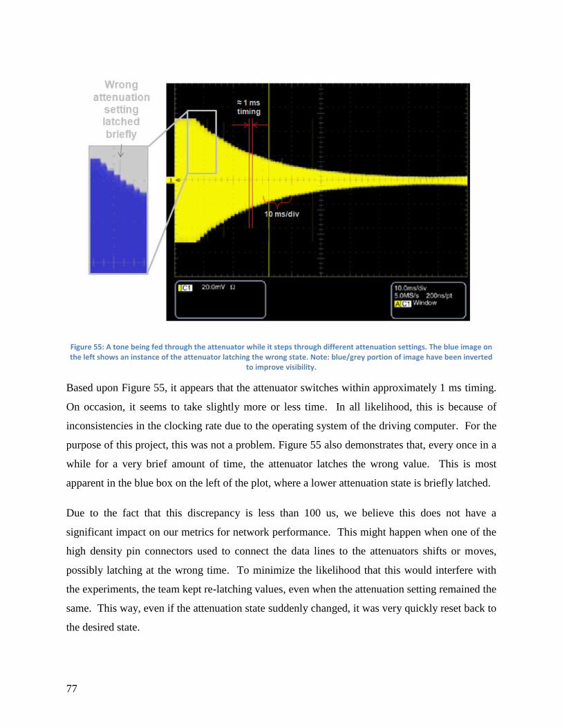
77

Figure 55: A tone being fed through the attenuator while it steps through different attenuation settings. The blue image on the left shows an instance of the attenuator latching the wrong state. Note: blue/grey portion of image have been inverted

to improve visibility.

Based upon Figure 55, it appears that the attenuator switches within approximately 1 ms timing.

On occasion, it seems to take slightly more or less time. In all likelihood, this is because of

inconsistencies in the clocking rate due to the operating system of the driving computer. For the

purpose of this project, this was not a problem. Figure 55 also demonstrates that, every once in a

while for a very brief amount of time, the attenuator latches the wrong value. This is most

apparent in the blue box on the left of the plot, where a lower attenuation state is briefly latched.

Due to the fact that this discrepancy is less than 100 us, we believe this does not have a

significant impact on our metrics for network performance. This might happen when one of the

high density pin connectors used to connect the data lines to the attenuators shifts or moves,

possibly latching at the wrong time. To minimize the likelihood that this would interfere with

the experiments, the team kept re-latching values, even when the attenuation setting remained the

same. This way, even if the attenuation state suddenly changed, it was very quickly reset back to

the desired state.

78

Krytar Coupler

Several qualities of the couplers were important to verify, including isolation between -3dB

ports, return loss looking into all three ports of interest, and the insertion loss of the device.

Measurements to characterize isolation between the two -3dB ports of the couplers were

conducted on the network analyzer. Isolation was measured across a 2 to 8 GHz band for two

different couplers. Results for the first coupler are shown in red and the second coupler is shown

in blue in Figure 56.

Figure 56: Isolation between -3dB ports of two different couplers. This measurement was taken from 2 to 8 GHz with the vector network analyzer.

The datasheet for the coupler specifies that isolation should greater than 18 dB. From Figure

55Figure 56: Isolation between -3dB ports of two different couplers. This measurement was

taken from 2 to 8 GHz with the vector network analyzer, it appears that the isolation between

ports is well above this. In fact, across the 2 GHz to 8 GHz band, the isolation is consistently

above 20 dB. In the Wi-Fi band, where the team did the majority of the experiments, the

isolation is greater than 30 dB.

79

Return loss was also measured on both -3dB ports and the sum port of the coupler. Results of

this measurement from 2 to 8 GHz are shown below in Figure 59. The red and blue lines are the

return loss at the two -3dB ports. The black line is the return loss measured at the sum port.

While the datasheet does not specify a return loss for any ports of the coupler, all three ports

seem to be above 15 dB. In the Wi-Fi band, return loss is greater than 25dB at all ports.

Figure 57: Coupler return loss, measured from 2 to 8 GHz. Return loss for each of the -3dB ports shown in red and blue. Return loss for sum port shown in black.

Coupler insertion loss was measured using the network analyzer for two different couplers. The

results for this measurement are shown in Figure 58. For each of the two couplers measured,

insertion loss was measured between the sum port and both of the -3dB ports. The first coupler

measured is shown in red, the second coupler measured is shown in blue.

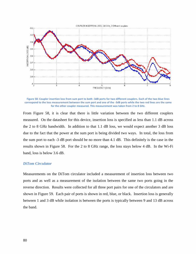
80

Figure 58: Coupler insertion loss from sum port to both -3dB ports for two different couplers. Each of the two blue lines correspond to the loss measurement between the sum port and one of the -3dB ports while the two red lines are the same

for the other coupler measured. This measurement was taken from 2 to 8 GHz.

From Figure 58, it is clear that there is little variation between the two different couplers

measured. On the datasheet for this device, insertion loss is specified as less than 1.1 dB across

the 2 to 8 GHz bandwidth. In addition to that 1.1 dB loss, we would expect another 3 dB loss

due to the fact that the power at the sum port is being divided two ways. In total, the loss from

the sum port to each -3 dB port should be no more than 4.1 dB. This definitely is the case in the

results shown in Figure 58. For the 2 to 8 GHz range, the loss stays below 4 dB. In the Wi-Fi

band, loss is below 3.6 dB.

DiTom Circulator

Measurements on the DiTom circulator included a measurement of insertion loss between two

ports and as well as a measurement of the isolation between the same two ports going in the

reverse direction. Results were collected for all three port pairs for one of the circulators and are

shown in Figure 59. Each pair of ports is shown in red, blue, or black. Insertion loss is generally

between 1 and 3 dB while isolation is between the ports is typically between 9 and 13 dB across

the band.

81

Figure 59: Circulator insertion loss (top) and isolation (bottom), measured from 2 to 8 GHz with network analyzer.

The insertion loss in the circulator appears to be consistently below 3 dB but not below the 1.5

dB specified on the datasheet. The datasheet also claims isolation provided is 10 dB minimum in

the 2 to 8 GHz range. This doesn’t seem to be the case in Figure 59, although in the Wi-Fi band,

isolation is no lower than 10 dB.

Figure 60: Return loss of DiTom circulator, measured from 2 to 8 GHz with network analyzer. Each different color represents one of the three different ports of the device.

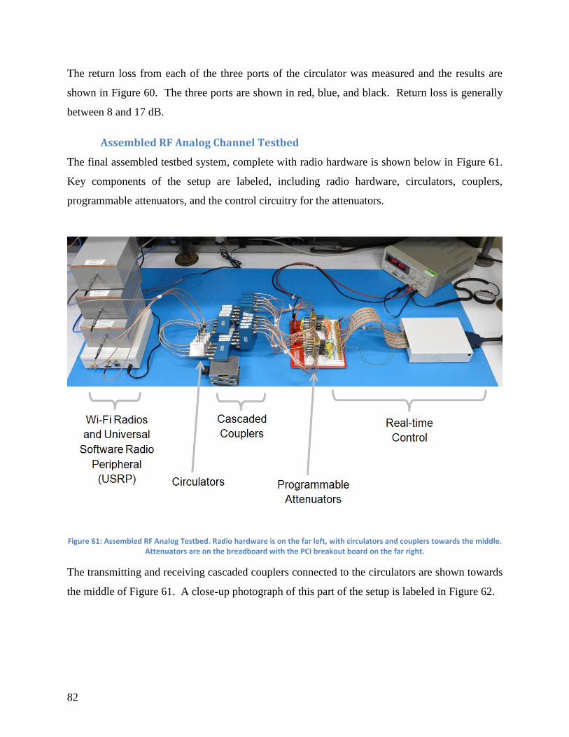
82

The return loss from each of the three ports of the circulator was measured and the results are

shown in Figure 60. The three ports are shown in red, blue, and black. Return loss is generally

between 8 and 17 dB.

Assembled RF Analog Channel Testbed

The final assembled testbed system, complete with radio hardware is shown below in Figure 61.

Key components of the setup are labeled, including radio hardware, circulators, couplers,

programmable attenuators, and the control circuitry for the attenuators.

Figure 61: Assembled RF Analog Testbed. Radio hardware is on the far left, with circulators and couplers towards the middle. Attenuators are on the breadboard with the PCI breakout board on the far right.

The transmitting and receiving cascaded couplers connected to the circulators are shown towards

the middle of Figure 61. A close-up photograph of this part of the setup is labeled in Figure 62.

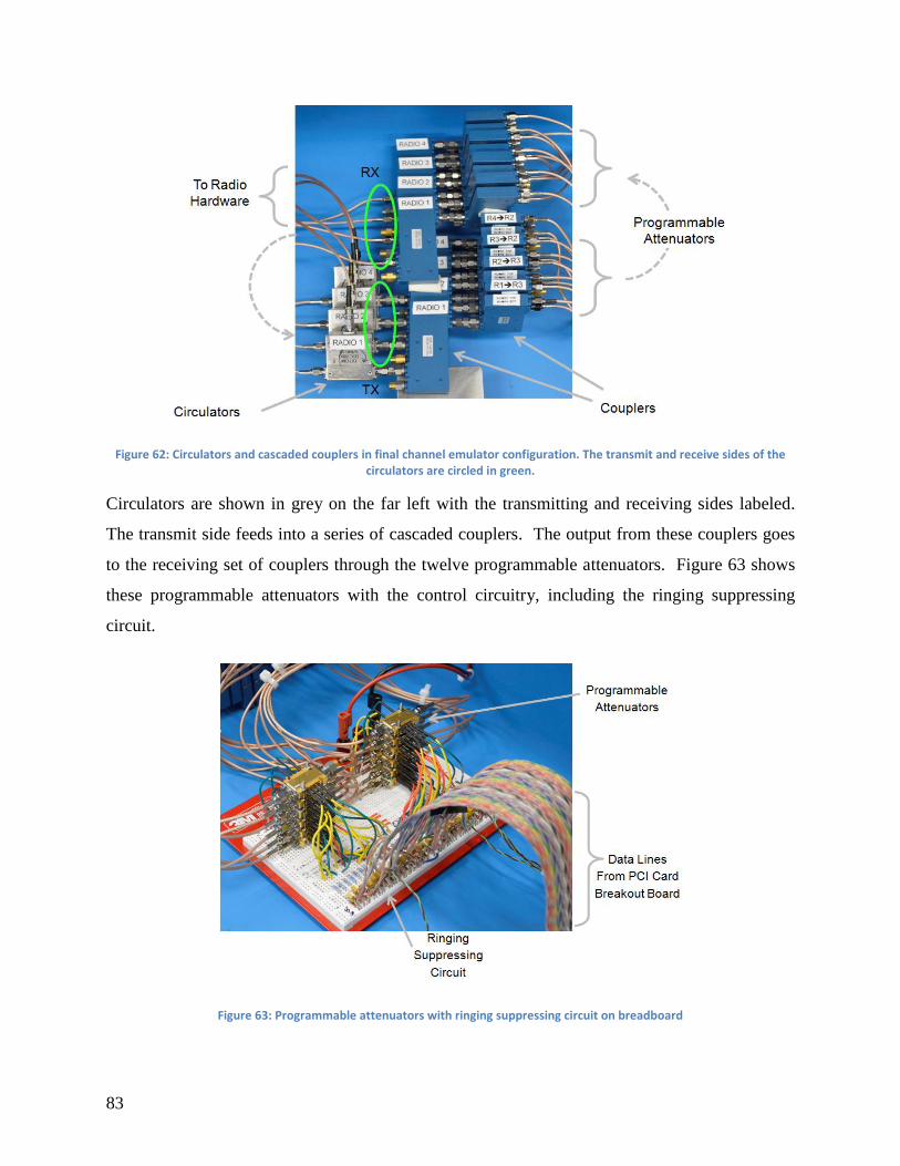
83

Figure 62: Circulators and cascaded couplers in final channel emulator configuration. The transmit and receive sides of the circulators are circled in green.

Circulators are shown in grey on the far left with the transmitting and receiving sides labeled.

The transmit side feeds into a series of cascaded couplers. The output from these couplers goes

to the receiving set of couplers through the twelve programmable attenuators. Figure 63 shows

these programmable attenuators with the control circuitry, including the ringing suppressing

circuit.

Figure 63: Programmable attenuators with ringing suppressing circuit on breadboard

84

The programmable attenuators are in two stacks of six, towards the left of Figure 63. The data

lines from the PCI card are in the bottom right of the image, each twisted with ground. The

breakout board is depicted in Figure 64.

Figure 64: SCB-68 NI breakout board closed (top) and open (bottom). Wires from this board are each twisted with a ground wire and connected to the attenuators on the breadboard.

The image in Figure 64 shows the breakout board, closed (top) and opened (bottom), for the NI

PCI card used to drive the attenuators.

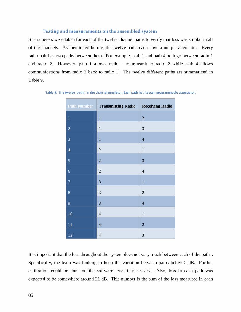
85

Testing and measurements on the assembled system

S parameters were taken for each of the twelve channel paths to verify that loss was similar in all

of the channels. As mentioned before, the twelve paths each have a unique attenuator. Every

radio pair has two paths between them. For example, path 1 and path 4 both go between radio 1

and radio 2. However, path 1 allows radio 1 to transmit to radio 2 while path 4 allows

communications from radio 2 back to radio 1. The twelve different paths are summarized in

Table 9.

Table 9: The twelve 'paths' in the channel emulator. Each path has its own programmable attenuator.

Path Number Transmitting Radio Receiving Radio

1 1 2

2 1 3

3 1 4

4 2 1

5 2 3

6 2 4

7 3 1

8 3 2

9 3 4

10 4 1

11 4 2

12 4 3

It is important that the loss throughout the system does not vary much between each of the paths.

Specifically, the team was looking to keep the variation between paths below 2 dB. Further

calibration could be done on the software level if necessary. Also, loss in each path was

expected to be somewhere around 21 dB. This number is the sum of the loss measured in each

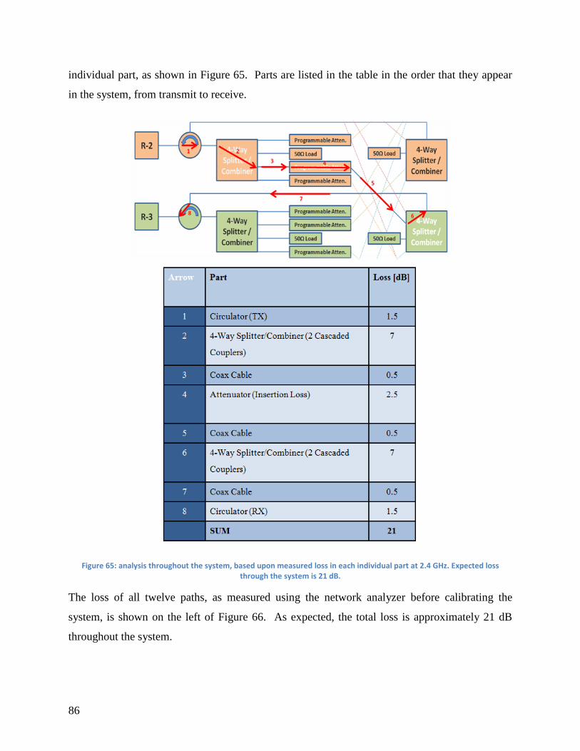
86

individual part, as shown in Figure 65. Parts are listed in the table in the order that they appear

in the system, from transmit to receive.

Figure 65: analysis throughout the system, based upon measured loss in each individual part at 2.4 GHz. Expected loss through the system is 21 dB.

The loss of all twelve paths, as measured using the network analyzer before calibrating the

system, is shown on the left of Figure 66. As expected, the total loss is approximately 21 dB

throughout the system.

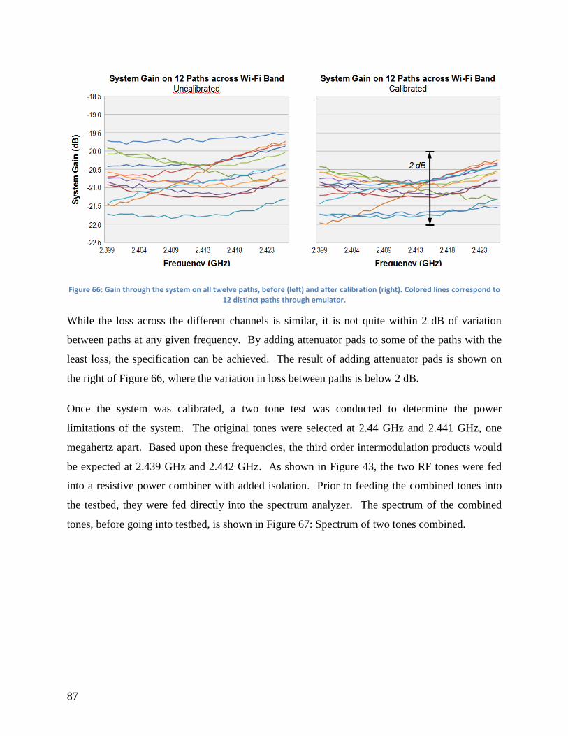
87

Figure 66: Gain through the system on all twelve paths, before (left) and after calibration (right). Colored lines correspond to 12 distinct paths through emulator.

While the loss across the different channels is similar, it is not quite within 2 dB of variation

between paths at any given frequency. By adding attenuator pads to some of the paths with the

least loss, the specification can be achieved. The result of adding attenuator pads is shown on

the right of Figure 66, where the variation in loss between paths is below 2 dB.

Once the system was calibrated, a two tone test was conducted to determine the power

limitations of the system. The original tones were selected at 2.44 GHz and 2.441 GHz, one

megahertz apart. Based upon these frequencies, the third order intermodulation products would

be expected at 2.439 GHz and 2.442 GHz. As shown in Figure 43, the two RF tones were fed

into a resistive power combiner with added isolation. Prior to feeding the combined tones into

the testbed, they were fed directly into the spectrum analyzer. The spectrum of the combined

tones, before going into testbed, is shown in Figure 67: Spectrum of two tones combined.

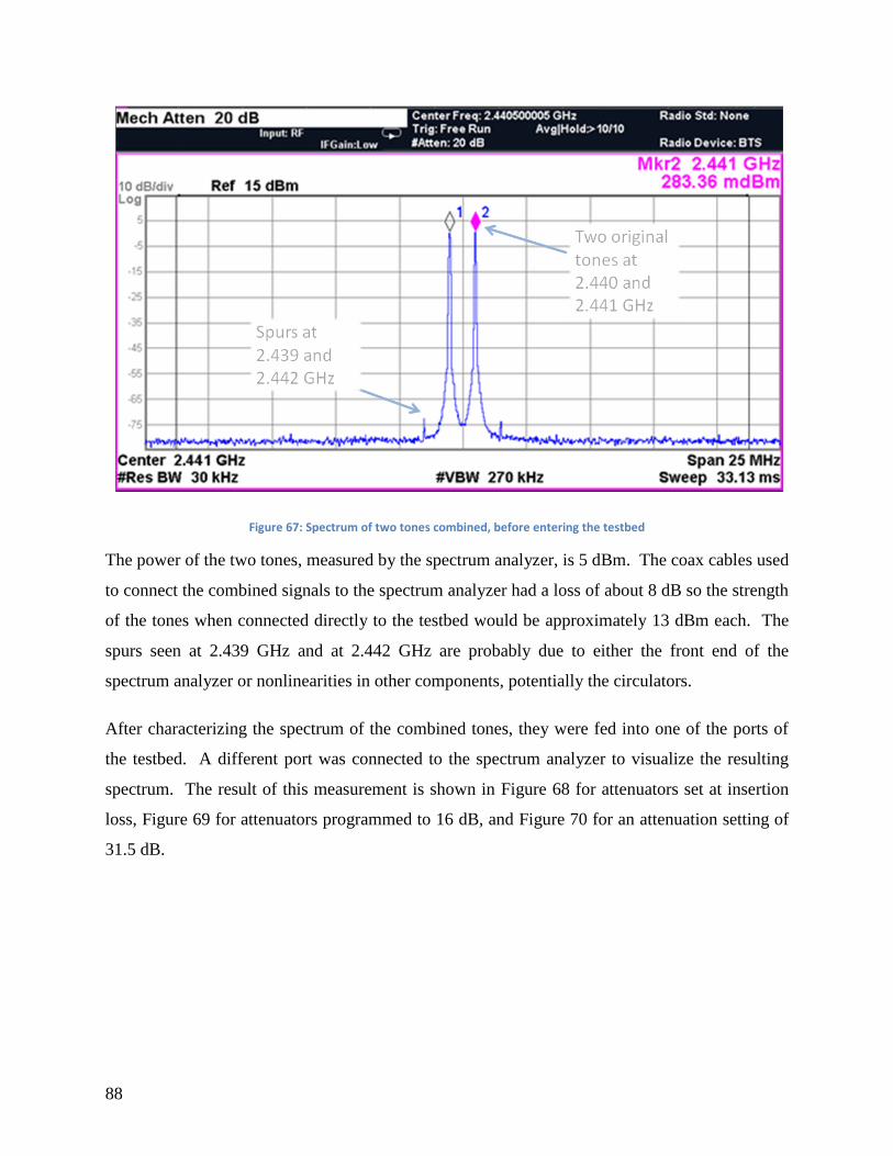
88

Figure 67: Spectrum of two tones combined, before entering the testbed

The power of the two tones, measured by the spectrum analyzer, is 5 dBm. The coax cables used

to connect the combined signals to the spectrum analyzer had a loss of about 8 dB so the strength

of the tones when connected directly to the testbed would be approximately 13 dBm each. The

spurs seen at 2.439 GHz and at 2.442 GHz are probably due to either the front end of the

spectrum analyzer or nonlinearities in other components, potentially the circulators.

After characterizing the spectrum of the combined tones, they were fed into one of the ports of

the testbed. A different port was connected to the spectrum analyzer to visualize the resulting

spectrum. The result of this measurement is shown in Figure 68 for attenuators set at insertion

loss, Figure 69 for attenuators programmed to 16 dB, and Figure 70 for an attenuation setting of

31.5 dB.

89

Figure 68: Two tones through the system, attenuators set to insertion loss

Figure 69: Two tones through the system, attenuators set to 16 dB setting

90

Figure 70: Two tones through the system, attenuators set to 31.5 dB setting

In this test, the power in the signal generators was turned up to the maximum allowable strength,

and we did not observe any spurs. In order to verify that this is a reasonable result, the team used

the third order input intercept point provided on the datasheet to back-calculate for the power

expected at the third order intercept products, assuming the attenuator is the primary source of

intermodulation distortion. Based upon this calculation, the team found that the power expected

at the third order intercept points would be well below the noise floor, so the measured results

make sense.

The purpose of this experiment was to verify that any intermodulation products were suitably

below the threshold for our experiment. Since the radios used in this experiment can operate at

an SNR as low as 20 dB, the team does not expect any problems. To better describe this system,

more powerful tones might be fed into the testbed so that the intermodulation products might be

observed above the noise floor. However, since we had limited time and the available signal

generators were turned to maximum power, we were unable to pursue this level of testing.

The team also repeated a published PHY layer DoS attack on a two radio network similar to the

one described in the literature [7]. Results of the repeated two radio network are shown in Figure

94, Figure 95, and Figure 96 in the Appendix. Once results similar to the paper were obtained on

91

the two radio network, the same tests were repeated on the four radio channel emulator to ensure

functionality. None of these tests use the mobility aspect of the channel emulator. These tests

confirmed that our testing parameters were acceptable measures of network operability. Results

of these experiments are below, including pulse, sweep, and digital jamming.

There were some differences between the two and four radio networks but these can be

explained due to the differences in equipment, hardware, and software. We begin with

comparing pulse jamming tests with the two radio testbed, and then the four radio testbed in

Figure 71.

Figure 71: Pulse Jamming tests: Throughput vs. Pulse length & period in Two Radio (A) testbed at 11Mbit/sec (DSSS), 9Mbit/sec (OFDM), and on the Four Radio testbed (B) at 11Mbit/sec (DSSS), 9Mbit/sec (OFDM).

The two radio testbed provides verification and validation of the procedure, equipment, and

analysis of the listed jamming techniques. Each experiment is a direct replication of peer-

reviewed research obtained from reputable sources [7], using similar software and hardware.

Shown in Figure 71, the pulse lengths (left column) are varied between 100 µS to 1000 µS, and

92

pulse periods are varied between 1 mS and 10 mS. If the pulse length and period are equal, the

jammer is continuous (bottom right corner).

When comparing Figure 71 (A) with (B) we notice that the results between the tests beds are

similar, although the four radio testbed shows an overall 7% increase in throughput compared

with the previous testbed. This is displayed clearly in Figure 73 which examines the differences

in performance observed between the two and four radio testbed. Sweep jamming results are

shown in Figure 72.

Figure 72: Sweep Jamming tests: Throughput vs. SJR & Sweep time in Two Radio testbed (A) at 11Mbit/sec (DSSS), 9Mbit/sec (OFDM), and on the Four Radio testbed (B) at 11Mbit/sec (DSSS), 9Mbit/sec (OFDM). Results are in Mbit/sec. Signal to

Jammer Ratio (SJR) and sweep time are varied.

Figure 72 shows the effects when introducing a single sine wave swept across the entire Wi-Fi

band (100 MHz) in 0.5 to 20 seconds. This is accomplished using the HP Synthesized Sweeper

listed in Table 8. Figure 72 lists sweep times (left column) along with the signal to jammer ratio

(SJR). The four radio testbed shows a slight decrease in jammer performance compared to the

two radio testbed. An SJR of 10 dB in the two radio testbed shows almost no effect on

throughput, while the four radio testbed shows 17% reduction in throughput.

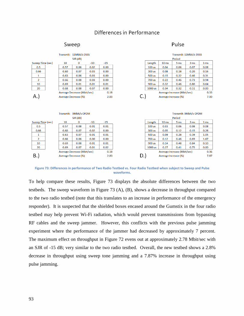
93

Figure 73: Differences in performance of Two Radio Testbed vs. Four Radio Testbed when subject to Sweep and Pulse waveforms.

To help compare these results, Figure 73 displays the absolute differences between the two

testbeds. The sweep waveform in Figure 73 (A), (B), shows a decrease in throughput compared

to the two radio testbed (note that this translates to an increase in performance of the emergency

responder). It is suspected that the shielded boxes encased around the Gumstix in the four radio

testbed may help prevent Wi-Fi radiation, which would prevent transmissions from bypassing

RF cables and the sweep jammer. However, this conflicts with the previous pulse jamming

experiment where the performance of the jammer had decreased by approximately 7 percent.

The maximum effect on throughput in Figure 72 evens out at approximately 2.78 Mbit/sec with

an SJR of -15 dB; very similar to the two radio testbed. Overall, the new testbed shows a 2.8%

decrease in throughput using sweep tone jamming and a 7.87% increase in throughput using

pulse jamming.

94

Digital jamming on the two radio testbed was implemented using MATLAB Simulink and its

UHD toolbox. Due to a loss of software during a computer crash, the digital jamming technique

was implemented on a readily available version of GNURadio. This may help to explain some

differences in the results, in particular the SJR at which throughput reaches zero, shown in

Figure 74.

Figure 74: Digital Jamming tests: Throughput vs. SJR on the Two Radio testbed using MATLAB (A) and Four Radio testbed using GNURadio (B) using 11 Mbit/sec DSSS and 9 Mbit/sec OFDM.

Figure 74 shows digital jamming (pseudo random DBPSK at 2.4 GHz) against DSSS (Blue) and

OFDM (Red). The previous testbed shows zero throughput at an SJR of 2 dB (Figure 74 (A),

circled in Red), while the new testbed shows zero throughput at an SJR of 8 dB (Figure 74 B,

circled in Red). When first attempting the experiment, we found that transmissions would cease

at an unexpected SJR of 20 dB. After altering excess bandwidth settings on GNURadio, this

point changed to 8 dB. This may suggest that the excess bandwidth or power produced using

GNURadio is enough to drop throughput at a much lower SJR than when using MATLAB.

95

Nearing the end of the project an opportunity arose that enabled us to test this theory. The

experiment was repeated using MATLAB with the emergency responder. Results are displayed

in Figure 75.

Figure 75: Digital Jamming tests (Corrected): Throughput vs. SJR on the Two Radio testbed using MATLAB (A) and Four Radio testbed using MATLAB (B) using 11 Mbit/sec DSSS and 9 Mbit/sec OFDM.

After repeating the Digital jamming test in Figure 74 using MATLAB with the emergency

responder in the four channel testbed, we found the results between the two testbeds to be within

10% error. A slight increase in the performance of the jammer is observed as throughput halts at

a higher SJR in Figure 75 (B) than (A). Additionally, the power spectrum density (PSD) was

recorded ~6 dB less when using MATLAB compared to GNURadio. This confirms our

hypothesis stated earlier that the increase in performance in Figure 74 (B) was a direct result of

the substitution of GNURadio for MATLAB.

According to work by Harjula et. al., [7], there should exist some difference in performance

against digital jamming between DSSS and OFDM, as OFDM resembles a digital-like signal and

96

would be more susceptible to digital jamming than DSSS, which slightly resembles noise. The

lack of separation between DSSS and OFDM suggests that the Gumstix Wi-Fi radios may be

changing modulation schemes. In other words, the Wi-Fi radio may be selecting whether to use

802.11b or 802.11g depending on signal conditions, even though they are strictly configured by

the user. We explore this question in Figure 76.

Figure 76: Spectrum of OFDM (9 Mbit/sec, 802.11g) signal (A) and with the addition of a Digital jammer (B). The graph in (A) shows a typical flat, OFDM signal modulation. The graph in (B) shows the OFDM modulation changing to a DSSS-like signal

when a Digital jammer is introduced.

This experiment examines the spectrum of Wi-Fi signals using the signal analyzer listed in Table

8 before and after a Digital jammer is introduced in the network. Each Wi-Fi radio is set to use

802.11g at 9 Mbit/s using the iwconfig utility. Figure 76 (A) shows a typical Wi-Fi transmission;

the spectrum is semi-flat at its peak, a characteristic of OFDM and 802.11g. A Digital jammer is

introduced with equal power (0 SJR), and begins to interfere with communication between the

two radios. What we notice is a drop in throughput and occasionally, the spectrum of the signal

changes to a round shape, a characteristic of 802.11b. Occasionally, ‘clipping’ effects may

appear when viewing the spectrum as in Figure 76 (B); this is likely an effect caused by the slow

sweep pattern of the signal analyzer. Our team made attempts to minimize this effect, but in the

interest of showing the best possible explanation some clipping was acceptable.

97

We propose two possible explanations; the jammer effectively breaks communication between

both nodes, and each node subsequently and repeatedly sends beacon packets (which look

similar to 802.11b signals). Or, the Gumstix radios are self-configuring their own modulation,

using 802.11b or 802.11g when it deems necessary. However, combined with the information

obtained from Figure 77, it is likely that the radio is self-configuring its modulation.

Figure 77: Spectrum of DSSS (11 Mbit/sec, 802.11b) signal (A) and with the addition of a Digital jammer (B). The graph in (A) shows a typical DSSS signal modulation. The graph in (B) shows the DSSS modulation changing to an OFDM-like signal when

a Digital jammer is introduced.

This experiment is similar to the previous except we first transmit data using 802.11b at 11

Mbit/sec (DSSS) (set using the iwconfig utility). Figure 77 (A) shows a typical 802.11b

spectrum. Then, we introduce a Digital jammer in Figure 77 (B). Notice how the spectrum

changes shape this time to a flat, OFDM shaped spectrum. It is worth noting that after taking

several samples, the flat-shaped spectrum samples were only a small percentage of the 802.11b

shaped samples. In other words, the radio primarily relies on 802.11b, but occasionally we can

see the 802.11g modulation being used. This behavior was observed only with the addition of an

interferer, suggesting that it may be switching modulation to increase performance against

interference. Again, these results imply that the differences noted in the testbed when compared

to previously published research (Figure 94, found the Appendix), are due to the self-configuring

adaptation of the Gumstix’ Wi-Fi radios when subject to interference.

98

4.2 Wi-Fi mobile jamming experiments

This section is primarily focused on the ability to accurately simulate distance between radio

nodes over time. Mobility is demonstrated by the results of the following experiments.

Additionally, we examined the differences between digital, pulse, and sweep jamming

techniques in equidistant, hidden, and distant node mobile scenarios. To further understand the

results, note the flow of traffic shown in Figure 78.

Figure 78: Flow of data in mobile experiments. All mobile data shown in graphs are transmitted in one direction by the prior node.

It is possible to transmit between every node, however this is difficult with Iperf as there is no

way to discern where the traffic originates. Therefore, we decided to use one direction of traffic

through each node. Radio 1 will transmit data to Radio 2 (Red), Radio 2 transmits to Radio 3

(Green), and Radio 3 transmits to Radio 1 (Blue). All nodes will use the same standard of color

throughout the following figures. Using this method the throughput between each radio link can

be measured. Note that the following Digital jamming experiments are shown using GNURadio

not MATLAB, and reflect the gain in power when using GNURadio, discussed in earlier in

Figure 74 and Figure 75.

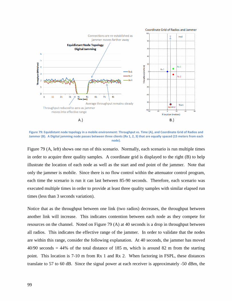
99

Figure 79: Equidistant node topology in a mobile environment: Throughput vs. Time (A), and Coordinate Grid of Radios and Jammer (B). A Digital jamming node passes between three clients (Rx 1, 2, 3) that are equally spaced (15 meters from each

node).

Figure 79 (A, left) shows one run of this scenario. Normally, each scenario is run multiple times

in order to acquire three quality samples. A coordinate grid is displayed to the right (B) to help

illustrate the location of each node as well as the start and end point of the jammer. Note that

only the jammer is mobile. Since there is no flow control within the attenuator control program,

each time the scenario is run it can last between 85-90 seconds. Therefore, each scenario was

executed multiple times in order to provide at least three quality samples with similar elapsed run

times (less than 3 seconds variation).

Notice that as the throughput between one link (two radios) decreases, the throughput between

another link will increase. This indicates contention between each node as they compete for

resources on the channel. Noted on Figure 79 (A) at 40 seconds is a drop in throughput between

all radios. This indicates the effective range of the jammer. In order to validate that the nodes

are within this range, consider the following explanation. At 40 seconds, the jammer has moved

40/90 seconds = 44% of the total distance of 185 m, which is around 82 m from the starting

point. This location is 7-10 m from Rx 1 and Rx 2. When factoring in FSPL, these distances

translate to 57 to 60 dB. Since the signal power at each receiver is approximately -50 dBm, the

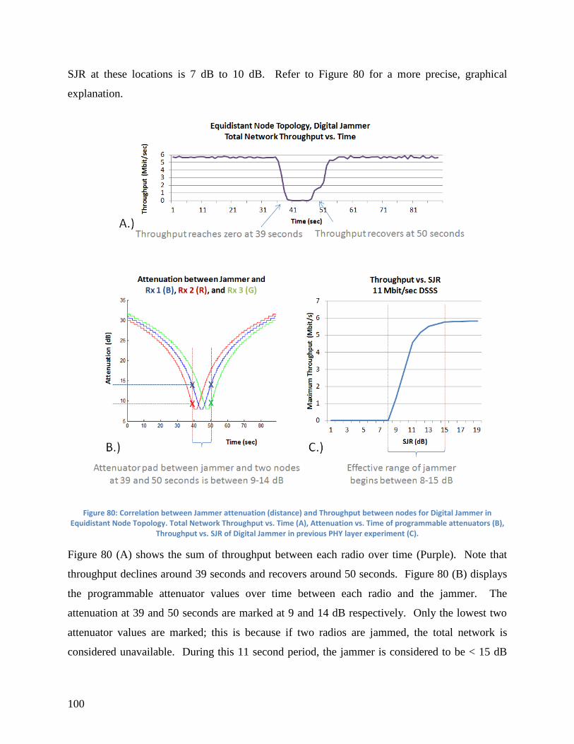
100

SJR at these locations is 7 dB to 10 dB. Refer to Figure 80 for a more precise, graphical

explanation.

Figure 80: Correlation between Jammer attenuation (distance) and Throughput between nodes for Digital Jammer in Equidistant Node Topology. Total Network Throughput vs. Time (A), Attenuation vs. Time of programmable attenuators (B),

Throughput vs. SJR of Digital Jammer in previous PHY layer experiment (C).

Figure 80 (A) shows the sum of throughput between each radio over time (Purple). Note that

throughput declines around 39 seconds and recovers around 50 seconds. Figure 80 (B) displays

the programmable attenuator values over time between each radio and the jammer. The

attenuation at 39 and 50 seconds are marked at 9 and 14 dB respectively. Only the lowest two

attenuator values are marked; this is because if two radios are jammed, the total network is

considered unavailable. During this 11 second period, the jammer is considered to be < 15 dB

101

from the radio nodes. According to previous PHY layer results in Figure 74, total throughput

during this period is expected to be from 0 to 5 Mbit/sec. When comparing these values to

Figure 80 (C), it is easy to see at 39 - 50 seconds the jammer has reached its effective range of 0-

15 dB, and throughput has ceased. Figure 81 displays the same Equidistant scenario with a pulse

jammer.

Figure 81: Equidistant node topology in a mobile environment: Throughput vs. Time (A), and Coordinate Grid of Radios and Jammer (B). A Pulse jamming node passes between three clients (Rx 1, 2, 3) that are equally spaced (15 meters from each

node).

The only variation in this experiment is the substitution for a Pulse jammer. The first data point

in Figure 81 (A) indicates high throughput from Rx 2 to Rx 3 (Green). When starting the

experiment, the first node will attempt to transmit while no other clients are on the network.

This contention free period allows high throughput, but is short-lived. In Figure 81 (A)

throughput decreases in the following order: Rx 2, Rx 1, Rx 3. This has a correlation to the

proximity of the jammer as it reaches these nodes in the same order. Nodes recover in a similar

pattern as the jammer leaves the vicinity with Rx 1 receiving the first transmission, although one

would expect Rx 2 to recover first.

102

To show an effective drop in network throughput the pulse jammer had been modified to

transmit approximately 75% of the time. The exact value in Mbit/sec was not previously

recorded in the PHY layer experiments; however the expected value is between 1.0 - 3.8

Mbit/sec at 0 SJR. In Figure 82 we examine the correlation between the total network

throughput and the jammer’s effective range.

Figure 82: Correlation between Jammer attenuation (distance) and Throughput between nodes for Pulse Jammer in Equidistant Node Topology. Total Network Throughput vs. Time (A), Attenuation vs. Time of programmable attenuators (B),

Throughput vs. Pulse Length vs. Pulse Period of Pulse Jammer in previous PHY layer experiment (C).

In terms of throughput over time the pulse jammer in Figure 82 (A) shows similar behavior to

the Digital jammer, although throughput (Teal) never totally reaches zero. Noticeable declines

in throughput are marked starting at 39 seconds, ending at 50 seconds. Figure 82 (B) indicates

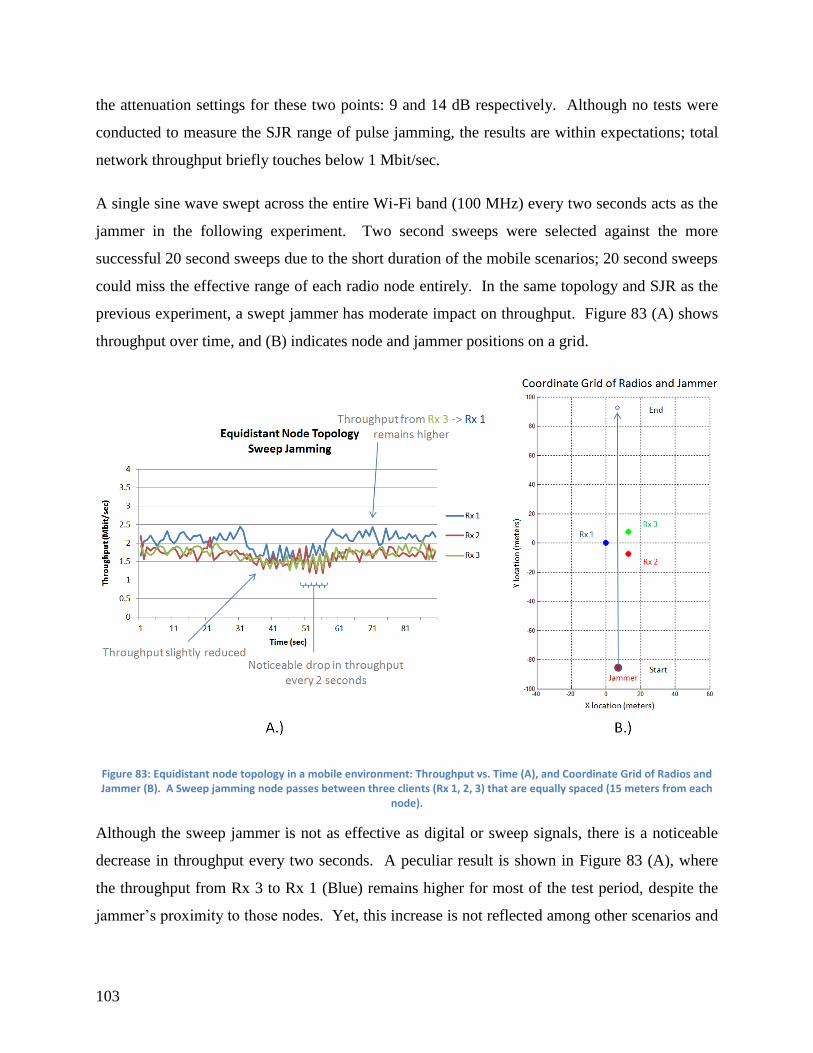
103

the attenuation settings for these two points: 9 and 14 dB respectively. Although no tests were

conducted to measure the SJR range of pulse jamming, the results are within expectations; total

network throughput briefly touches below 1 Mbit/sec.

A single sine wave swept across the entire Wi-Fi band (100 MHz) every two seconds acts as the

jammer in the following experiment. Two second sweeps were selected against the more

successful 20 second sweeps due to the short duration of the mobile scenarios; 20 second sweeps

could miss the effective range of each radio node entirely. In the same topology and SJR as the

previous experiment, a swept jammer has moderate impact on throughput. Figure 83 (A) shows

throughput over time, and (B) indicates node and jammer positions on a grid.

Figure 83: Equidistant node topology in a mobile environment: Throughput vs. Time (A), and Coordinate Grid of Radios and Jammer (B). A Sweep jamming node passes between three clients (Rx 1, 2, 3) that are equally spaced (15 meters from each

node).

Although the sweep jammer is not as effective as digital or sweep signals, there is a noticeable

decrease in throughput every two seconds. A peculiar result is shown in Figure 83 (A), where

the throughput from Rx 3 to Rx 1 (Blue) remains higher for most of the test period, despite the

jammer’s proximity to those nodes. Yet, this increase is not reflected among other scenarios and

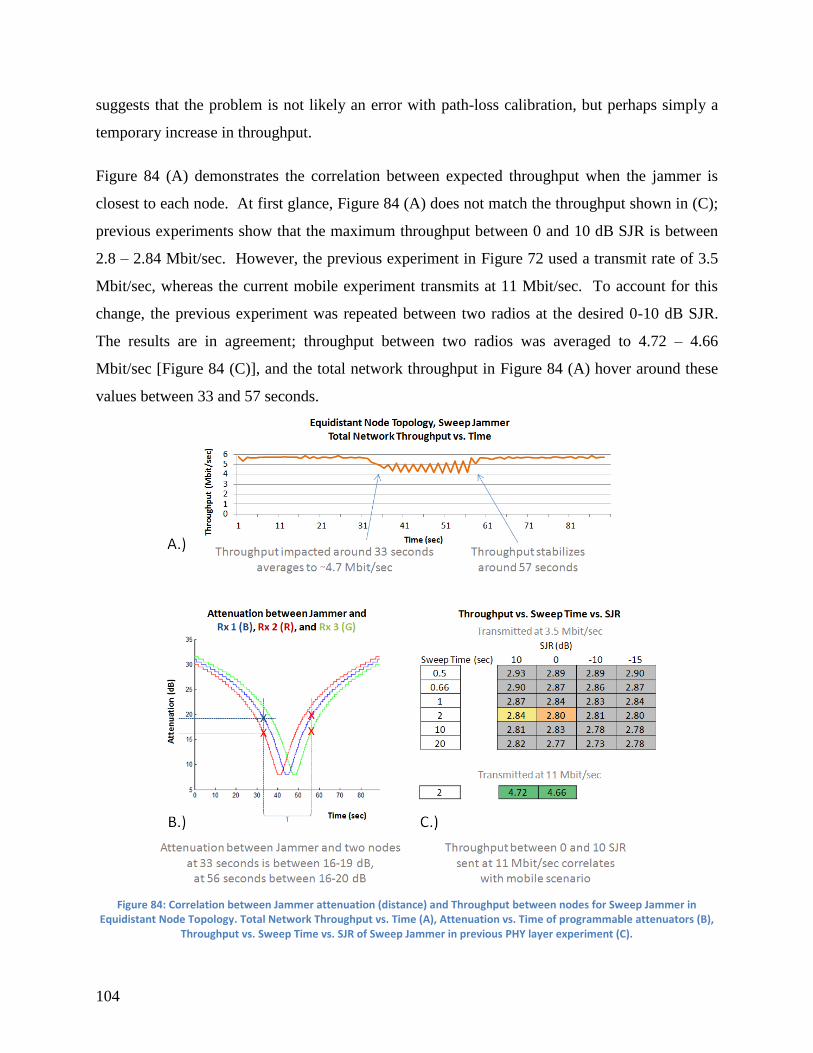
104

suggests that the problem is not likely an error with path-loss calibration, but perhaps simply a

temporary increase in throughput.

Figure 84 (A) demonstrates the correlation between expected throughput when the jammer is

closest to each node. At first glance, Figure 84 (A) does not match the throughput shown in (C);

previous experiments show that the maximum throughput between 0 and 10 dB SJR is between

2.8 – 2.84 Mbit/sec. However, the previous experiment in Figure 72 used a transmit rate of 3.5

Mbit/sec, whereas the current mobile experiment transmits at 11 Mbit/sec. To account for this

change, the previous experiment was repeated between two radios at the desired 0-10 dB SJR.

The results are in agreement; throughput between two radios was averaged to 4.72 – 4.66

Mbit/sec [Figure 84 (C)], and the total network throughput in Figure 84 (A) hover around these

values between 33 and 57 seconds.

Figure 84: Correlation between Jammer attenuation (distance) and Throughput between nodes for Sweep Jammer in Equidistant Node Topology. Total Network Throughput vs. Time (A), Attenuation vs. Time of programmable attenuators (B),

Throughput vs. Sweep Time vs. SJR of Sweep Jammer in previous PHY layer experiment (C).

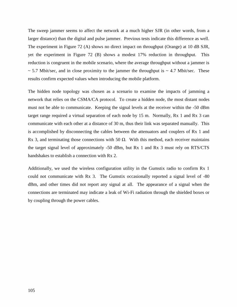
105

The sweep jammer seems to affect the network at a much higher SJR (in other words, from a

larger distance) than the digital and pulse jammer. Previous tests indicate this difference as well.

The experiment in Figure 72 (A) shows no direct impact on throughput (Orange) at 10 dB SJR,

yet the experiment in Figure 72 (B) shows a modest 17% reduction in throughput. This

reduction is congruent in the mobile scenario, where the average throughput without a jammer is

~ 5.7 Mbit/sec, and in close proximity to the jammer the throughput is ~ 4.7 Mbit/sec. These

results confirm expected values when introducing the mobile platform.

The hidden node topology was chosen as a scenario to examine the impacts of jamming a

network that relies on the CSMA/CA protocol. To create a hidden node, the most distant nodes

must not be able to communicate. Keeping the signal levels at the receiver within the -50 dBm

target range required a virtual separation of each node by 15 m. Normally, Rx 1 and Rx 3 can

communicate with each other at a distance of 30 m, thus their link was separated manually. This

is accomplished by disconnecting the cables between the attenuators and couplers of Rx 1 and

Rx 3, and terminating those connections with 50 Ω. With this method, each receiver maintains

the target signal level of approximately -50 dBm, but Rx 1 and Rx 3 must rely on RTS/CTS

handshakes to establish a connection with Rx 2.

Additionally, we used the wireless configuration utility in the Gumstix radio to confirm Rx 1

could not communicate with Rx 3. The Gumstix occasionally reported a signal level of -80

dBm, and other times did not report any signal at all. The appearance of a signal when the

connections are terminated may indicate a leak of Wi-Fi radiation through the shielded boxes or

by coupling through the power cables.

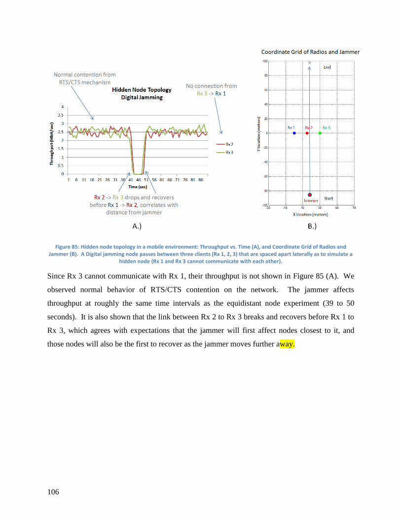
106

Figure 85: Hidden node topology in a mobile environment: Throughput vs. Time (A), and Coordinate Grid of Radios and Jammer (B). A Digital jamming node passes between three clients (Rx 1, 2, 3) that are spaced apart laterally as to simulate a

hidden node (Rx 1 and Rx 3 cannot communicate with each other).

Since Rx 3 cannot communicate with Rx 1, their throughput is not shown in Figure 85 (A). We

observed normal behavior of RTS/CTS contention on the network. The jammer affects

throughput at roughly the same time intervals as the equidistant node experiment (39 to 50

seconds). It is also shown that the link between Rx 2 to Rx 3 breaks and recovers before Rx 1 to

Rx 3, which agrees with expectations that the jammer will first affect nodes closest to it, and

those nodes will also be the first to recover as the jammer moves further away.

107

Figure 86: Hidden node topology in a mobile environment: Throughput vs. Time (A), and Coordinate Grid of Radios and Jammer (B). A Pulse jamming node passes between three clients (Rx 1, 2, 3) that are spaced apart laterally as to simulate a


This experiment exhibits a shorter jamming duration, with throughput recovering more quickly

than with digital jamming. As the jammer approaches around 36 seconds, there is a noticeable

separation in throughput between Rx 2 to Rx 3 (Green) compared to the link from Rx 1 to Rx 2

(Red). This effect is seen in all hidden node scenarios and shows that even though the jammer is

only 3 meters closer to Rx 3 than Rx 1, it appears to have an impact on the network.

108

Figure 87: Hidden node topology in a mobile environment: Throughput vs. Time (A), and Coordinate Grid of Radios and Jammer (B). A Sweep jamming node passes between three clients (Rx 1, 2, 3) that are spaced apart laterally as to simulate a


We observed an increased range of performance when using a Sweep waveform; notice the

periodic drop in throughput in Figure 87 (A) is evident beginning around 30 seconds, which is

around 10 seconds earlier (~20 m ahead), where the link is also slow to recover. The sweep

jammer may be able to disturb MAC layer protocols more effectively than other waveforms,

which would explain its ability to affect throughput at a greater distance.

Preparation for a distant node scenario is similar to the hidden node experiment in that the link

between the two furthest nodes is broken; in this case, Rx 3 to Rx 1. The connection between the

programmable attenuators and couplers between Rx 1 and Rx 3 were left untouched with a 50 Ω

termination from the hidden node experiment.

In Figure 88 (A) it is clear that the jammer affects Rx 3 (Green) within the first 10 seconds. The

throughput received at Rx 2 (Red) reaches only 5 Mbit/sec of the typical maximum 5.8 Mbit/sec.

This virtual ceiling may be due to the overhead of attempted retransmissions of Rx 2 while Rx 3

is unavailable, in combination with a longer distance (thus, smaller data rate). Figure 93

109

indicates a reduced maximum throughput between all hidden and distant node scenarios, which

seem to support this theory.

Figure 88: Distant node topology in a mobile environment: Throughput vs. Time (A), and Coordinate Grid of Radios and Jammer (B). A Digital jamming node passes between three clients (Rx 1, 2, 3); Rx 3 is isolated and can only communicate

with Rx 2 from a longer distance.

There is a noticeable loss in throughput between Rx 1 to Rx 2 (Red), and an increase in

throughput between Rx 2 to Rx 3 (Green). This is likely due to the sudden availability of Rx 3

as the jammer is not within effective range of any node, followed by a loss in throughput at node

Rx 2. As expected, the link between Rx 2 to Rx 3 recovers before the link between Rx 1 to Rx 2

(at approximately 61 seconds).

Figure 88 (A) shows that the maximum throughput achieved by Rx 2 to Rx 3 is less than the

throughput achieved by Rx 1 to Rx 2, which is also expected since throughput decreases with

distance. However, the results of the next experiment conflict with this theory; the data rate

between both links average out towards the end of the test, shown in Figure 89 (A).

110

Figure 89: Distant node topology in a mobile environment: Throughput vs. Time (A), and Coordinate Grid of Radios and Jammer (B). A Pulse jamming node passes between three clients (Rx 1, 2, 3); Rx 3 is isolated and can only communicate with

Rx 2 from a longer distance.

Figure 89 (A) shows different behavior from the beginning of the experiment. These differences

are subtle; refer to Figure 93 for a clearer comparison between jamming techniques. We

observed a similar contention point at 41 seconds, although it appears as though the signal from

Rx 1 to Rx 2 (Red) is strong enough to dominate the spectrum. At about 60 seconds, we notice

that the link from Rx 1 to Rx 2 breaks down, but quickly recovers while the link from Rx 2 to Rx

3 is delayed, unlike the digital jammer in Figure 88 (A). This may be due to the weakness of the

pulse jammer to effectively prevent Rx 1 from communicating with Rx 2.

Additionally, throughput averages out between both links to the same value of 2.5 Mbit/sec after

75 seconds, unlike Figure 88. The fact that both links can achieve equal throughput suggests that

Rx 3 is not far away enough to lose a contention for resources. The next experiment involves a

sweep jammer in the same distant node topology.

111

Figure 90: Distant node topology in a mobile environment: Throughput vs. Time (A), and Coordinate Grid of Radios and Jammer (B). A Sweep jamming node passes between three clients (Rx 1, 2, 3); Rx 3 is isolated and can only communicate

with Rx 2 from a longer distance.

The effectiveness of a Sweep jammer at these specifications is questionable (100 MHz sweep

range of a 22 MHz channel). However, we do notice some effect from the Sweep jammer at a

very early stage. This is in agreement with our experimental results, as the sweep jammer

achieves a 15% reduction in throughput from only 10 dB SJR, it is likely to have a smaller effect

from 15-20 dB SJR.

An interesting point of this graph is the reduction in throughput at the receiver of Rx 2, yet no

reduction at Rx 3. Even though the jammer reaches the same proximity to all nodes, it is not

powerful enough to decrease throughput beyond 2.5 Mbit/sec, and since Rx 3 is already limited

in throughput (from a distance), the jammer has little effect on this node. Compared to other

techniques, each jammer’s performance is varied, as shown in Figure 91.

112

Figure 91: Comparison of performance among different jamming techniques in a mobile, Equidistant node topology. Graph of Total Network Throughput vs. Time of Digital, Pulse, and Sweep jamming.

Digital jamming (Purple) clearly shows improved performance over the Pulse (Teal) and Sweep

(Orange) methods. Maximum throughput matches results from previous experiments: around

5.7-5.8 Mbit/sec average without presence of a jammer. Pulse jamming results also agree with

results taken from previous experiments: nearly 1 Mbit/sec at close range of the jammer. A

sweep tone with a range only across channel 1 of Wi-Fi 802.11b/g may show increased

performance and perhaps the ability to interfere with enough packets to cause a disconnection or

disassociation between nodes.

113

Figure 92: Comparison of performance among different jamming techniques in a mobile, Hidden node topology. Graph of Total Network Throughput vs. Time of Digital, Pulse, and Sweep jamming.

Total throughput in Figure 92 is approximately 5 Mbit/sec, compared to 5.8 Mbit/sec in the

Equidistant node topology. The reduction in throughput may be due to the added overhead when

relying on a middle node. The sweep jammer seems to have less of an effect, but a wider range

of variability; another indication of its ability to affect communications with high SJR, most

likely by affecting the MAC layer.

However, since the two radio testbed results of sweep tone jamming are similar to results

produced by Harjula et. al., indicating an effect with an SJR < 10 dB, the values shown in Figure

92 remain an undefined anomaly of the four radio testbed as it suggests a range of SJR > 10 dB.

114

Figure 93: Comparison of performance among different jamming techniques in a mobile, Distant node topology. Graph of Total Network Throughput vs. Time of Digital, Pulse, and Sweep jamming.

From Figure 93, we see a definitive separate in performance from sweep jamming, but the digital

and pulse techniques show a split in performance at two intervals. At 21 seconds and 73 seconds

the effectiveness of the digital and pulse jammers alternate, implying that a Pulse jammer is more

effective against distant nodes from greater than 10 meters, but a Digital jammer is more

effective at closer ranges.

Overall we observed mostly predictable behavior with a few discrepancies. It was predicted and

later verified that the mobile jammer would affect the radio nodes according to its effective range

derived from the PHY layer experiments. However, even though we used different software

(substituted GNURadio for MATLAB) in the digital jamming experiment, we did not expect

such a dramatic increase in effective range (6-7 dB). This was explained and confirmed in

Figure 74 and Figure 75 by the increase in bandwidth of signals produced by GNURadio as

opposed to MATLAB.

It was unexpected to see a slight increase in performance of sweep and digital jamming.

Although, these gains could be explained by the addition of shielded boxes and the placement of

copper tape along power cables in the four radio testbed (the previous two radio testbed had no

115

shielding over the Gumstix) which help to reduce Wi-Fi radiation and consequently prevent

signals from bypassing the jammer, but this does not explain the decreased performance of pulse

jamming.

4.2.1 MAC Layer Mobile Jamming

We began testing the theory that repeated beacons would have an impact on network throughput.

Approximately four seconds of typical beacon traffic between three nodes was captured using

GNURadio and the USRP. This data was then played back into a wireless card connected to a

computer with Linux: Backtrack. A tool called “horst” (Highly Optimized Radio Spectrum

Tool) confirmed that the packets being transmitted were legitimate. Additionally, we observed

the iwconfig utility on one single wireless node (unconnected to any network) which reported a

valid connection. This means that the process of recording and play-back of the wireless beacon

traffic was being correctly received.

Traffic was recorded when all three nodes were using WEP encryption and a 1 Mbit/s data rate.

Then, the network was modified to use no encryption and a 54 Mbit/s rate. We observed an

impact on throughput when this recording was played back into the network within a maximum

range of 15-20 dB SJR. However, we also transmitted pulsed noise designed to mimic the

wireless traffic but did not contain any useful information, and this had the same impact on

throughput. This means that the replayed beacons had the same impact as pulsed noise, and

suggest that the network is not affected by malicious beacon traffic.

On the contrary, it may be that the wireless nodes are rejecting these beacon packets as they are

not properly synced with their own beacons. Unfortunately, due to time constraints our team

was not able to completely explore the “reactive” portion of this experiment. We did find that

the Wireshark tool was not able to display management frames, and was not fast enough to

support reliable predictions of beacon traffic. In the future we would suggest aligning fake

beacon traffic to occur directly before or after the target’s beacon, at which time the target would

be more likely to accept the new information as it aligns with other beacons. This could be

implemented using UHD tools instead of GNURadio, which would offer a much faster response

time.

116

5 Conclusions and Future Work

The RF channel emulator designed, built, and tested in this project provided a suitable testing

platform for PHY layer jamming techniques on a mobile configuration of radios. Results from

testing and validation indicate that the testbed is functional and representative of a simplified RF

channel. In addition, results from the mobile PHY layer jamming experiments suggest that the

testbed is a viable platform for investigating jamming methods and techniques. Its mid-range

price tag achieves an economical balance between the high fidelity of hardware systems and the

repeatability of wireless channel emulators. The demonstration of the MAC layer attack was

unsuccessful; a repeated beacon signal did not seem to have an effect on network performance,

however this topic was not fully explored. Finally, while the testbed served the purposes and

scope of the project, the team has identified several improvements and alterations that could

increase accuracy and robustness. In this chapter, key conclusions will be described followed by

areas identified for additional work and development.

The tests on various components and the system as a whole indicated that the testbed designed

and built over the course of this project meets specifications and is fully functional. As

originally defined, key specifications for the testbed included attenuator switching speed less

than 1 ms, isolation greater than 20 dB between different paths, less than 45 dB loss through the

system, and no greater than 2 dB of variation in loss between those paths. As shown in the

results and discussion chapter, these specifications have been met.

In general, the testbed performed to specification based upon testing. It also performed well in

the validation testing done. In order to verify the functionality of the testbed, the team repeated

some stationary PHY layer experiments from a publication by Harjula e.al [Citation!] and

compared results. When results were compared with this published research, the team findings

contained an acceptable amount of error which could otherwise be explained by the substitution

of equipment and software. This served as a validation of the testbed, confirmed testing

procedure, and provided a benchmark for future mobile scenarios.

Our research into the performance and effects of various jamming techniques in a mobile

environment produced expected results; in most scenarios, digital jamming remains the most

effective against 802.11 receivers, compared to pulse and sweep jamming. Yet, these findings

117

are preliminary. Additional research using wireless cards that offer enhanced control and

flexibility (for instance the ability to definitively control modulation, data rate, transmit power,

and MAC layer controls) would allow for selective tests that target specific layers of the 802.11

protocol and could help to answer how each technique affects communications while moving.

While the team did not ultimately have enough time for any conclusive testing on the MAC layer

beacon frame attack, some preliminary testing was completed. The ‘reactive’ portion of the

technique was found to be challenging due to timing limitations, so beacons were instead

replicated without precise timing. The team found that replicating a client’s beacon frame using

false encryption and data rates did not severely affect network performance. A noticeable drop

in throughput was observed, but this is likely correlated to collisions from transmitting beacon

packets. It is possible that other nodes on the network are rejecting these false packets. Future

work in this area could implement a truly reactive beacon to confirm this theory.

Although the channel emulator met testing requirements for this project, there are several steps

that could be taken to improve its utility as a long term test asset. For example, although the

testbed is designed to support testing from 2 to 8 GHz, it is only calibrated for the Wi-Fi band.

Extending calibration over the entire band would make the testbed useful for a wider variety of

testing scenarios. An even larger bandwidth could be supported if the 30 MHz to 3 GHz parts

are added to the system as discussed in the methodology. Some enhancements might also be

added that could improve the range of mobile situations that can be represented on the testbed.

Currently, the testbed supports changing geometries where each node starts and ends at a

specified location and moves between those two locations during the simulation in a straight line

at a constant rate over a specified run time. A more complicated scenario might involve motion

beyond just a straight line. More sophisticated MATLAB code would enable this type of

experiment. A GUI which prompts users for information regarding node placement and then

generates corresponding graphic depicting the moving nodes might also improve the usability of

the testbed.

In addition to increasing the number of testing scenarios supported by the testbed, system

durability and robustness could be improved with further work. One potential area for

improvement involves the attenuator driving mechanism. In the current setup, the attenuators are

118

driven by an NI PCI card connected to a breadboard through a breakout board. An FPGA might

offer cleaner signals and more flexibility. The breadboard itself is not the best long term setup.

Replacing that with a more permanent structure with soldered connections might reduce any

problems due to the temporary nature of the high density pin connectors.

In summary, the team constructed a functional, four node, 2 – 8 GHz channel emulator calibrated

over the Wi-Fi band. This channel emulator was used to test a series of mobile jamming

techniques in three different scenarios. The team found that digital jamming shows an increased

ability to negatively affect network performance when compared with pulse and sweep

techniques, except in distant node topologies where pulse jamming displays better performance

at a distance greater than 10 meters.

Our increased reliance on wireless communications, especially in crowded public safety bands,

underlies the importance of spectrum reallocation for use by emergency responders during a

crisis. The ability to utilize a calibrated, wireless, mobile test environment is critical to those

who wish to alleviate the problem of congested networks. We hope that continued development

of flexible test platforms, such as the channel emulator described in this report, will contribute to

effective re-establishment of communications by emergency responders and authorized

personnel in the event of a natural disaster.

119

6 References

[1] The Guardian, "Tsunami report criticises relief effort," 5 10 2005. [Online]. Available:

http://www.guardian.co.uk/world/2005/oct/05/internationalaidanddevelopment.tsunami2004

. [Accessed 2 10 2012].

[2] T. W. House, "The Federal Reponse to Hurricane Katrina: Lessons Learned," 2006.

[3] Satellite Today, "Proactive Measures Needed When it Comes to Communications," 3 10

2005. [Online]. Available: http://www.satellitetoday.com/via/features/Proactive-Measures-

Needed-When-It-Comes-To-Communications_278.html. [Accessed 2 10 2012].

[4] A. M. Townsend and M. L. Moss, "Telecommunications Infrastructure in Disasters," New

York University: Center for Catasrophe Preparedness and Response, 2005.

[5] A. Bogan, "DHS Official Says Cell Phone Emergency Service Failed During Eastern

Quake," ExecutiveGov, 29 Nov 2011. [Online]. Available:

www.executivegov.com/2011/11/dhs-official-says-cell-phone-emergency-service-failed-

during-eastern-quake/. [Accessed 3 September 2012].

[6] F. C. Commission, "Public Safety/Private Partnership," Public Safety and Homeland

Security Bureau, [Online]. Available: transition.fcc.gov/pshs/public-safety-spectrum/700-

MHz/partnership.html. [Accessed 3 September 2012].

[7] I. Harjula, J. Pinola and J. Prokkola, "Performance of IEEE 802.11 Based WLAN Devices

Under Various Jamming Signals," VTT Technical Research Centre of Finland, Oulu, 2011.

[8] R. Vaidya, C. Yadav, J. Kunkumath and P. Yadati, "Network Congestion Control:

Mechanisms for Congestion Avoidance and Recovery," Juniper Networks, Bangalore, 2011.

[9] P. Hart, L. Heyse and A. Boin, "New Trends in Crisis Management Practice and Crisis

Management Research: Setting the Agenda," Journal of Contingencies and Crisis

Management, vol. 9, no. 4, p. 182, 2001.

[10] T. W. Coombs, Ongoing Crisis Communication, Thousand Oaks: SAGE Publications, Inc.,

2012.

[11] R. Miller, "Hurricane Katrina: Communications & Infrastructure Impacts," 2006. [Online].

Available:

www.carlisle.army.mil/DIME/documents/Hurricane%20Katrina%20Communications%20

&%20Infrastructure%20Impacts.pdf. [Accessed 3 9 2012].

120

[12] A. Kwasinski, "Effects of Notable Natural Disasters from 2005 to 2011 on

Telecommunications Infrastructure," University of Texas at Austin, Austin, 2011.

[13] R. C. Johnson, S. A. William and A. G. Klein, Software Receiver Design, Cambridge, UK:

Cambridge University Press, 2011.

[14] W. Stallings, Data and Computer Communications, Upper Saddle River, NJ: Prentice Hall,

2011.

[15] ADC Telecommunications Inc., "Modern Technology vs. HFC Ingress Noise," 1 March

2001. [Online]. Available: www.adc.com/us/en/Library/Literature/100327EC.pdf.

[16] P. De, S. Sharma and T. Chiueh, "Design considerations for a multihop wireless network

testbed," Communications Magazine, IEEE, pp. 102-109, 2005.

[17] T. Krop, M. Hollick, P. S. Mogre and R. Steinmetz, "A survey on real world and emulation

testbeds for mobile ad hoc networks," in Testbeds and REsearch Infrastructures for the

Development of Networks and Communities, Barcelona, 2006.

[18] S. Sanghani, T. Brown, S. Bhandare and S. Doshi, "EWANT: the emulated wireless ad hoc

network testbed," in Wireless Communications and Networking, New Orleans, 2003.

[19] K. Bialkowski and M. Portmann, "Design of testbed for wireless mesh networks," in

Antennas and Propagation Society International Symposium, Toronto, 2010.

[20] T. Clancy and B. Walker, "MeshTest: laboratory-based wireless testbed for large

topologies," in TridentCom 2007, Lake Buena, 2007.

[21] Rutgers University, "ORBIT - Wireless Network Testbed," 2012. [Online]. Available:

www.winlab.rutgers.edu/docs/focus/ORBIT.html.

[22] JFW Industries, "RF Matrix Switch Application Note," [Online]. Available:

http://www.jfwindustries.com/catalog/RF_Matrix_Switch_App_Note-111-1.html.

[23] G. Judd, D. D. Stancil and P. Steenkiste, "FPGA-Based Channel Simulator for a Wireless

Network Emulator," in Vehicular Technology Conference, Barcelona, 2009.

[24] Elektrobit, [Online]. Available: https://www.elektrobit.com/file.php?id=3038. [Accessed 20

September 2012].

[25] W. A. Arbaugh, N. Shankar and Y. J. Wan, "Your 802.11 Wireless Network has No

Clothes*," Department of Computer Science, University of Maryland, 2001.

[26] IEEE, "The IEEE Standards Association - 802.11i-2004," 2004. [Online]. Available:

121

http://standards.ieee.org/getieee802/download/802.11i-2004.pdf. [Accessed 23 8 2012].

[27] W. Chou, "Architecture Lecture Notes," 2004. [Online]. Available:

http://www4.ncsu.edu/~chou/course/LectureNotes/architecture.htm.

[28] K. Pahlavan and P. Krishnamurth, Principles of Wireless Networks, Prentice Hall, 2002.

[29] Agilent, "RF Testing of WLAN Products - Application Note 1380-1," 2007.

[30] J. Fakatselis and M. Belkerdid, "Processing Gain for Direct Sequence Spread Spectrum

Communication Systems and PRISMTM," Harris Semiconductor, 1996.

[31] R. A. Poisel, Modern Communications Jamming: Principles and Techniques, Norwood:

Artech House, 2011.

[32] Wi-Fi Alliance, "WiFi CERTIFIED n: Longer-Range, Faster-Throughput, Multimedia-

Grade WiFi Networks," 2009.

[33] J. DiMascio, "Jammers Causing Interference in Iraq," InsideDefense.com, 2006.

[34] National Instruments, "Two-Tone Third-Order Intermodulation Distortion Measurement,"

National Instruments, 15 March 2010. [Online]. Available: http://www.ni.com/white-

paper/4384/en. [Accessed 31 August 2012].

[35] E. Bayraktaroglu, C. King, X. Liu, G. Noubir, R. Rajaraman and B. Thapa, "Performance of

IEEE 802.11 under Jamming," 2010.

[36] P. Romano, "The Range vs. Rate Dilemma of WLANs," EE Times, 2004.

[37] B. Walker, I. Vo, M. Beecher and C. Clancy, "A demonstration of the MeshTest wireless

testbed," in TridentCom, Washington, DC, 2009.

[38] D. Raychaudhuri, I. Seskar, M. Ott, S. Ganu, K. Ramachandran, H. Kremo, R. Siracusa, H.

Liu and M. Singh, "Overview of the ORBIT radio grid testbed for evaluation of next-

generation wireless network protocols," in Wireless Communications and Networking

Conferance, 2005 IEEE, 2005.

[39] National Severe Storms Laboratory, "Questions and Answers about Lightning," 20 July

2009. [Online]. Available: http://www.nssl.noaa.gov/primer/lightning/ltg_climatology.html.

[40] National Instruments, "Testing Wireless Receivers with Recorded RF Spectrum," 2012.

[Online]. Available: image from http://zone.ni.com/devzone/cda/pub/p/id/197.

[41] Agilent Technologies, "Cascaded Noise Analysis," 2012. [Online]. Available:

122

http://edocs.soco.agilent.com/display/sv201001/Advanced+Spectrasys.

[42] M. Debbah, "Short Introduction to OFDM," Mobile Communications Group, 2004.

[43] "Gumstix," 2012. [Online]. Available: www.gumstix.com.

[44] R. C. Johnson, W. Sethares and A. G. Klein, Software Receiver Design, Cambridge, UK:

Cambridge University Press, 2011.

[45] D. M. Pozar, Microwave and RF Design of Wireless Systems, New York: John Wiley and

Sons, Inc., 2001.

[46] R. B. Ertel, P. Cadieri, K. W. Sowerby, T. S. Rappaport and J. H. Reed, "Overview of

Spatial Channel Models for Antenna Array Communication Systems," Personal

Communications, IEEE, vol. 5, no. 1, pp. 10-22, 1998.

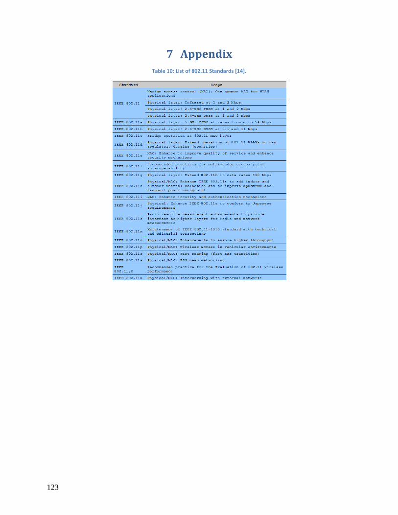
123

7 Appendix

Table 10: List of 802.11 Standards [14].

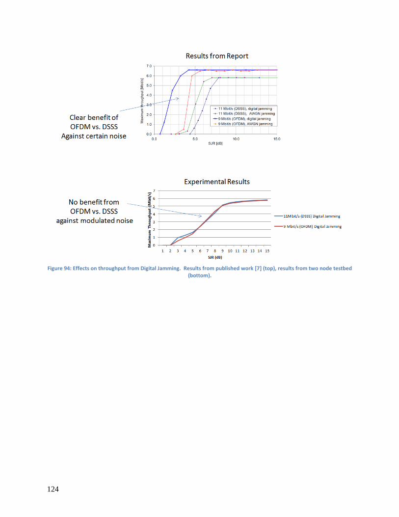
124

Figure 94: Effects on throughput from Digital Jamming. Results from published work [7] (top), results from two node testbed (bottom).

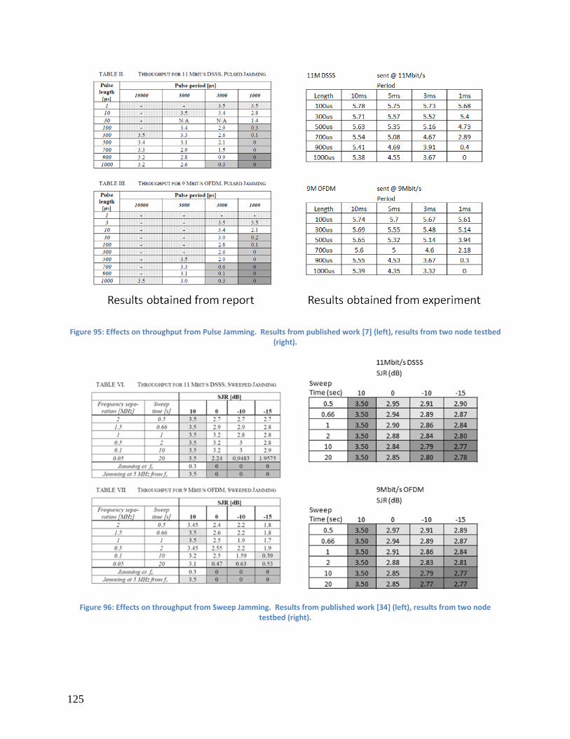
125

Figure 95: Effects on throughput from Pulse Jamming. Results from published work [7] (left), results from two node testbed (right).

Figure 96: Effects on throughput from Sweep Jamming. Results from published work [34] (left), results from two node testbed (right).

126

MATLAB Code: Calculate Programmable Attenuator Values

function [ attenuation_values ] = calc_att(start_vector,...

stop_vector, duration_s )

%CALC_ATT This function consumes a start_vector(4,1) with imaginary number

%components where the real part is the x location and the imaginary part is

%the y location. Stop vector is the same. Duration is the number of ms the

%experiment is meant to be run.

duration_ms = (1.6667*duration_s)*1000;

% figure out timing

num_ms = round(duration_ms);

time_vector = 0:1:(num_ms); %[ms]

time_vector = rot90(fliplr(time_vector));

att_pad_dB = 50.5;%SUBJECT TO CHANGE, this is the value of the additional

% attenuator pads in the system

delta = stop_vector - start_vector; %[meters]

velocity = delta./num_ms; %[meters/ms]

freq = 2.4; %[GHz]

position = ones(num_ms+1,4); %initialize

for a = 1:1:4

position(:,a) = rot90( real(velocity(a))*time_vector +real(start_vector(a))...

+ j* ( imag (velocity(a))*time_vector +imag(start_vector(a))));

end

distance = ones(num_ms+1, 6);

mult = [2 3 4 3 4 4; 1 1 1 2 2 3];

for b = 1:1:(num_ms+1) %rows-- num_ms

for c = 1:1:6 %columns-- specifies which column of mult to use

radioa = mult(1,c);

radiob = mult(2,c);

distance(b,c) = abs( position(b, radioa) - position( b, radiob) );

end

end

distance;

%attenuation_values = ones(num_ms, 6); %initialize

attenuation_values6 = 20*log10(distance/1000) + 20*log10(freq) + 94.45;

attenuation_values = ones(num_ms+1, 12);

%fill matrix

attenuation_values(:,1:3) = attenuation_values6(:,1:3);

attenuation_values(:,4) = attenuation_values6(:,1);

attenuation_values(:,5:6) = attenuation_values6(:,4:5);


127






attenuation_values = round((attenuation_values-att_pad_dB)*2)/2;

%Plotting the changing geometry and attenuation settings:

figure

subplot(1,2,2)

hold on

grid on

x = 0:1:1667;

plot(x,(attenuation_values(:,3)), 'b')

plot(x,(attenuation_values(:,6)), 'r')

plot(x,(attenuation_values(:,9)), 'g')

plot(x,(attenuation_values(:,1)), 'c')

plot(x,(attenuation_values(:,2)), 'k')

plot(x,(attenuation_values(:,5)), 'm')

title('Att. setting btwn jammer & radios 1(b) 2(r) and 3(g)')

ylabel('Attenuation between nodes [dB]');

xlabel('Time [s]');

set(gca, 'XTick', 0:187.4668:1668)

set(gca, 'XTickLabel', '0','10','20','30', '40', '50',...

'60', '70', '80', '90')

xlim([0 1667]);

hold off

subplot(1,2,1)

grid on

xlabel('X Location [meters]');

ylabel('Y Location [meters]');

title('Radio1 (b) Radio2 (r) Radio 3 (g) Jammer (moving)')

set(gca, 'YTick', -100:20:100)

set(gca, 'YTickLabel', '-100','-80','-60','-40','-20','0','20', '40', '60', '80' '100')

% hidden node

% xlim([-30 70])

% set(gca, 'XTick', -30:20:70)

% set(gca, 'XTickLabel', '-30','-10','10','30','50','70')

% equidistant & distant node

xlim([-40 60])

set(gca, 'XTick', -40:20:60)

set(gca, 'XTickLabel', '-40','-20','0','20','40','60')

hold on

scatter(7, 95, 1, 'y')

128

scatter(7, -95, 1, 'y')

hold on

scatter(real(position(:,1)),imag(position(:,1)), 100, 'b', 'filled')

hold on

scatter(real(position(:,2)),imag(position(:,2)), 100, 'r', 'filled');

hold on

scatter(real(position(:,3)),imag(position(:,3)), 100, 'g', 'filled');

comet(real(position(:,4)),imag(position(:,4)))

end

MATLAB Code: Generate ASCII Characters

function [] = gen_ascii3( attenuation_values )

%GEN_ASCII2 This function generates a matrix of ones and zeros to be sent

%to 12 attenuators and writes to a txt file named 'writefile.txt'

num_ms = length(attenuation_values(:,1));

% structure output matrix q

% each att value takes up 24 rows of a four column matrix.Att val switches

% every ms so:

q = ones((24*num_ms),15);

% initialize attenuation matrix, columns: C,R,L,S(12). Each attenuation

% matrix sets one set of values for all twelve attenuators

matrix = ones(24,15);

for n = 1:2:23

matrix(n,1)=0;

end

matrix(1:20,3) = 0;

matrix(3:4,2) = 0;

%This loop sets up the matrix for each value and puts it into q at the

%appropriate location

for i = 1:1:num_ms

%intitialize att bits

attenuation_bits = ones(12,12);

for j = 1:1:12 %this loop sets the attenuation bits,goes down x axis

a = round(attenuation_values(i,j)*2);

binary_rep = dec2bin(a,6);

%binary_rep = str2num(dec2bin( round(attenuation_values(i,j)*2) , 6 ))

for k = 1:1:6 %goes down the y axis of matrix filling in

l = 7-k;

b = not(str2num(binary_rep(l)));

attenuation_bits( ((2*k)-1):(2*k), j )= b;

end

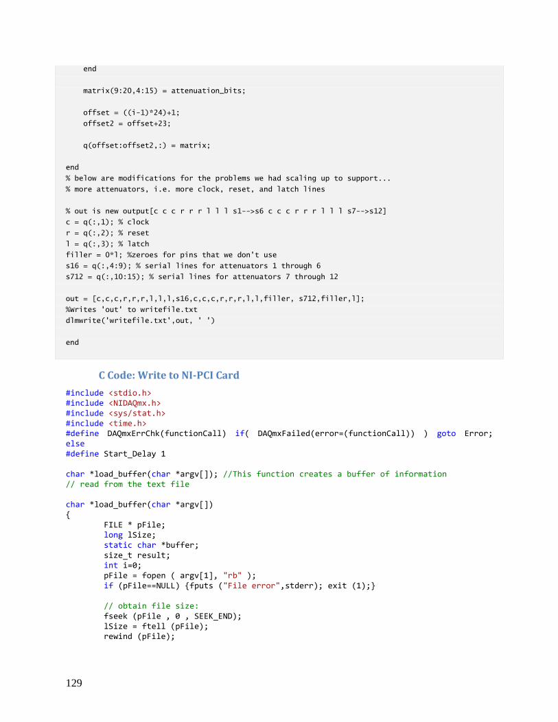
129

end

matrix(9:20,4:15) = attenuation_bits;

offset = ((i-1)*24)+1;

offset2 = offset+23;

q(offset:offset2,:) = matrix;

end

% below are modifications for the problems we had scaling up to support...

% more attenuators, i.e. more clock, reset, and latch lines

% out is new output[c c c r r r l l l s1-->s6 c c c r r r l l l s7-->s12]

c = q(:,1); % clock

r = q(:,2); % reset

l = q(:,3); % latch

filler = 0*l; %zeroes for pins that we don't use

s16 = q(:,4:9); % serial lines for attenuators 1 through 6

s712 = q(:,10:15); % serial lines for attenuators 7 through 12

out = [c,c,c,r,r,r,l,l,l,s16,c,c,c,r,r,r,l,l,filler, s712,filler,l];

%Writes 'out' to writefile.txt

dlmwrite('writefile.txt',out, ' ')

end

C Code: Write to NI-PCI Card

#include <stdio.h> #include <NIDAQmx.h> #include <sys/stat.h> #include <time.h> #define DAQmxErrChk(functionCall) if( DAQmxFailed(error=(functionCall)) ) goto Error; else #define Start_Delay 1 char *load_buffer(char *argv[]); //This function creates a buffer of information // read from the text file char *load_buffer(char *argv[]) FILE * pFile; long lSize; static char *buffer; size_t result; int i=0; pFile = fopen ( argv[1], "rb" ); if (pFile==NULL) fputs ("File error",stderr); exit (1); // obtain file size: fseek (pFile , 0 , SEEK_END); lSize = ftell (pFile); rewind (pFile);

130

// allocate memory to contain the whole file: buffer = (char*) malloc (sizeof(char)*lSize); if (buffer == NULL) fputs ("Memory error",stderr); exit (2); // copy the file into the buffer: result = fread (buffer,1,lSize,pFile); if (result != lSize) fputs ("Reading error",stderr); exit (3); /* the whole file is now loaded in the memory buffer. */ return buffer; int main(int argc, char *argv[]) // loops through the different lines of data writing them // to the card one line at a time // To use this program, type: // ./WriteDigChan_jeff file2write.txt -r // include -r if you want to write the file to the card on repeat int32 error=0; TaskHandle taskHandle=0; char errBuff[2048]='\0'; char Devstr[32] ; int i; int option_index = 0; char str1[]="Dev2/port0/line0:31"; strncpy(Devstr, str1, 32); char *buf = load_buffer(argv); sleep(Start_Delay); DAQmxErrChk (DAQmxCreateTask("",&taskHandle)); DAQmxErrChk (DAQmxCreateDOChan(taskHandle,Devstr,"",DAQmx_Val_ChanForAllLines)); DAQmxErrChk (DAQmxStartTask(taskHandle)); /*********************************************/ // DAQmx Write Code /*********************************************/ uInt8 output[32]; do char* ptr = &buf[0]; int temp_buffer[32]; while(*ptr != '\0') for (i=0;i<=31;i++) temp_buffer[i]=(int)(*ptr)-48; ptr++; ptr++; output[i]=(uInt8)temp_buffer[i]; // printf("%i ", output[i]); //printf("\n"); DAQmxErrChk (DAQmxWriteDigitalLines(taskHandle,1,1,10.0,DAQmx_Val_GroupByChannel,output,NULL,NULL)); int z; for (z=0;z<1000;z++)z=z; // seems to suppress clock delay problems while(argc==3 && strcmp(argv[2],"-r") == 0);

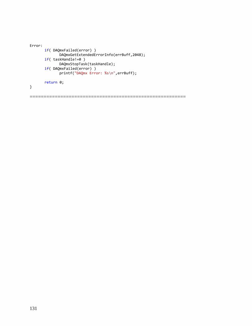
131

Error: if( DAQmxFailed(error) ) DAQmxGetExtendedErrorInfo(errBuff,2048); if( taskHandle!=0 ) DAQmxStopTask(taskHandle); if( DAQmxFailed(error) ) printf("DAQmx Error: %s\n",errBuff); return 0;

========================================================

132

Datasheet: Krytar Coupler

133

134

135

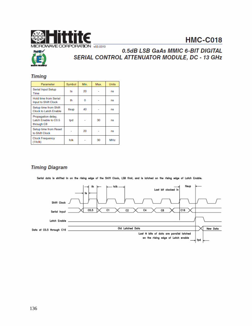
136

137

138

139

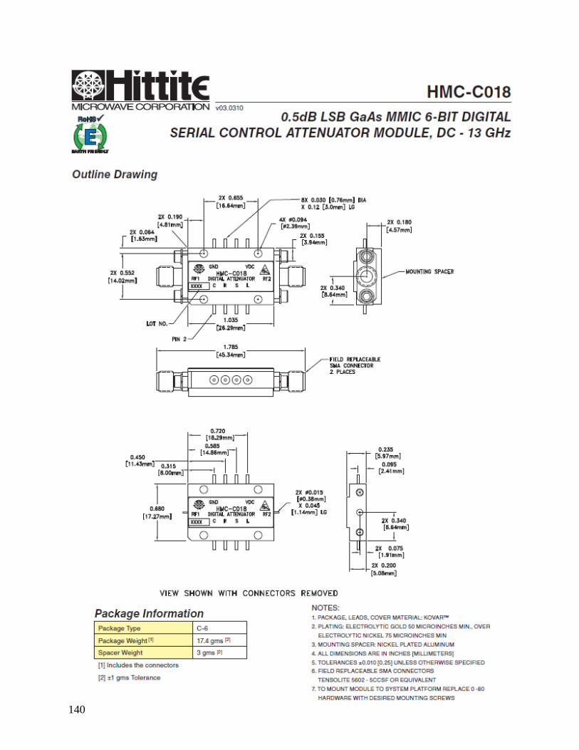
140

141

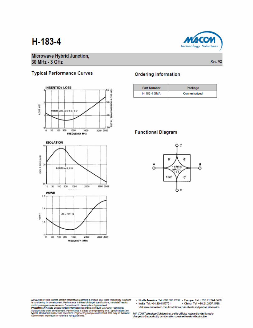
142

Documents

Wi-Fi Denial of Service Attack on Wired Analog RF … · Wi-Fi Denial of Service Attack on Wired Analog RF ... and a software defined radio called a Universal Software Radio Peripheral