FINAL REPORT

Wide Area Augmentation System Research and Development

Frank van Graas, Ph.D. Principal Investigator

February 2004

Avionics Engineering Center School of Electrical Engineering and Computer Science

Russ College of Engineering and Technology Ohio University

Athens, Ohio

Prepared under: Federal Aviation Administration Cooperative Agreement 01-G-016

2

TABLE OF CONTENTS Page LIST OF FIGURES 3 LIST OF TABLES 4 EXECUTIVE SUMMARY 5 1.0 INTRODUCTION 6 2.0 CODE NOISE AND MULTIPATH MONITOR 7 3.0 GEOSTATIONARY SATELLITE MULTIPATH ERROR

CHARACTERIZATION 12

3.1 Flight Test Processing 13 3.2 Douglas Dakota DC-3 Flight Test Results 15 3.3 Piper Saratoga Flight Test Results 22 4.0 PROTOTYPE DUAL-FREQUENCY INTEGRATED MULTIPATH-

LIMITING ANTENNA 25

4.1 Dual-Frequency High-Zenith Antenna (HZA) 27 4.2 Dual-Frequency Dipole-Array Multipath-Limiting Antenna

(MLA) 29

5.0 GPS ANTENNA PHASE AND GROUP DELAYS 31 5.1 Antenna Calibration Requirements 33 5.2 Importance of Group Delays for WAAS and LAAS 34 5.3 Measurement of Antenna Group Delay 35 5.3.1 Sensitivity of antenna range group delay to phase

measurement noise 35

5.3.2 Comparison of antenna range and CMC-derived group delays

35

5.4 Calibration Methodology 38 5.5 Compact Antenna Range Measurements 40 5.6 Case Study: High-Zenith Antenna Calibration 41 6.0 SUMMARY OF RESEARCH RESULTS 45 7.0 REFERENCES 46

3

LIST OF FIGURES Page Figure 2-1. CNMP Monitor Principles 7 Figure 2-2. Example Multipath Threat Model 10 Figure 3-1. Double Difference Geometry 14 Figure 3-2. Ohio University’s DC-3 Research Aircraft (N7AP) 15 Figure 3-3. Aircraft Ground Track for the Flight Test on September

26, 2001 16

Figure 3-4. Satellite Skyplot for the Flight Test on September 26, 2001 17 Figure 3-5. CMC for PRN 29; Aircraft (top); Ground (bottom) 17 Figure 3-6. CMC for PRN 122 (AOR-W); Aircraft (top); Ground

(bottom) 18

Figure 3-7. DC-3 Aircraft Antenna Installation 19 Figure 3-8. PR (top) and AD (bottom) Double Differences for PRNs

20 and 29 20

Figure 3-9. PR (top) and AD (bottom) Double Differences for PRNs 29 and 122 (GEO)

20

Figure 3-10. Ohio University’s Piper Saratoga Research Aircraft (N8238C)

22

Figure 3-11. Aircraft Ground Track for the Flight Test on September 13, 2002

23

Figure 3-12. CMC Residuals for PRN 25 (Elevation ~76 degrees) 23 Figure 3-13. CMC Residuals for PRN 14 (Elevation ~45 degrees) 24 Figure 4-1. Dual-Frequency High-Zenith Antenna (from [4]) 28 Figure 4-2. High-Zenith Antenna D/U Performance at L1 (red, top

curve), L2 (blue, middle curve), and Design Goal (black, constant line at 20 dB)

28

Figure 4-3. Dipole Array Elements (from [4]) 29 Figure 4-4. Dipole Array MLA D/U Performance at L1 (red, top

curve), L2 (blue, middle curve), and Design Goal (black, constant line at 20 dB)

30

Figure 5-1. Example of LAAS Smoothed Pseudorange in the Presence of Phase Delays

34

Figure 5-2. CMC Processing Retains the Group Delay Signature 37 Figure 5-3. Antenna Range Measurement Geometry 38 Figure 5-4. Compact Radar Measurement Range 40 Figure 5-5. High-Zenith Antenna on the Compact Radar

Measurement Range 41

Figure 5-6. Compact Range Measurement Geometry 41 Figure 5-7. Ground Multipath D/U for High Zenith and PinWheel

Antennas 42

Figure 5-8. HZA Phase and Group Delays as a Function of Polarization

43

Figure 5-9. Installed High-Zenith (left) and PinWheel (right) Antennas

43

Figure 5-10. CMC Results for High-Zenith and PinWheel Antennas 44

4

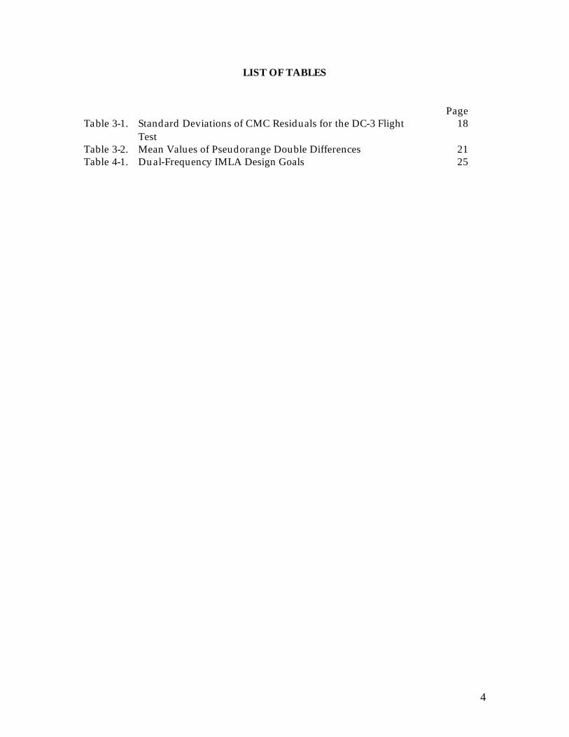
LIST OF TABLES Page Table 3-1. Standard Deviations of CMC Residuals for the DC-3 Flight

Test 18

Table 3-2. Mean Values of Pseudorange Double Differences 21 Table 4-1. Dual-Frequency IMLA Design Goals 25

5

EXECUTIVE SUMMARY In support of the development of the Wide Area Augmentation System (WAAS), three projects were performed under Aviation Cooperative Agreement 01-G-016. The first project involved participation in the WAAS Integrity Performance Panel (WIPP), which included the development of the dual-frequency Code Noise and MultiPath (CNMP) monitor, review of integrity documentation, as well as the analysis of specific integrity monitors. The second project was focused on the characterization and reduction of Geostationary Satellite (GEO) multipath error. The third project involved the development of a dual-frequency Integrated Multipath-Limiting Antenna (IMLA) for WAAS Reference Sites (WRS) to improve the accuracy of the pseudorange measurement data. Major findings of the research are summarized below:

1) A dual-frequency Code Noise and MultiPath (CNMP) monitor was developed to significantly reduce multipath error at the WAAS Reference Sites (WRS).

2) Based on ground and flight test evaluations, Narrow-Band Geostationary Satellite (GEO) multipath and noise ranging errors can be as small as 0.3 m (95%) if a multipath-limiting High-Zenith Antenna (HZA) is used.

3) A dual-frequency Integrated Multipath-Limiting Antenna (IMLA) was prototyped and determined to be feasible for WAAS applications.

4) A new method was developed for the measurement and evaluation of GPS antenna phase and group delays.

6

1.0 INTRODUCTION In support of the development of the Wide Area Augmentation System (WAAS), three projects were performed under Aviation Cooperative Agreement 01-G-016. The first project involved participation in the WAAS Integrity Performance Panel (WIPP), which included the development of the Code Noise and MultiPath (CNMP) monitor, review of integrity documentation, as well as the analysis of specific integrity monitors. The second project was focused on the characterization and reduction of Geostationary Satellite (GEO) multipath error. The third project involved the prototyping of a dual-frequency Integrated Multipath-Limiting Antenna (IMLA) for WAAS Reference Sites (WRS) to improve the accuracy of the pseudorange measurement data. The need for the CNMP monitor originated from the WIPP meetings, where data collection results showed relatively large multipath errors that negatively affected the performance of the differential corrections. The CNMP monitor is documented in Section 2.0. To improve the utility of the Inmarsat, narrow-band Geostationary Satellites (GEOs), a project was initiated to characterize and reduce the multipath error on the GEO signals as received at the WRS. Section 3.0 details the characterization methodology, which includes both ground and flight tests. Design, prototyping and test results of a dual-frequency, Integrated Multipath-Limiting Antenna (IMLA) for potential use in the WRS are presented in Section 4.0. Section 5.0 contains a description of a new methodology to measure and correct for GPS antenna phase and group delays.

7

2.0 CODE NOISE AND MULTIPATH MONITOR A new method was developed to reduce the code noise and multipath error on the pseudorange measurements at the WRS. This method uses the real-time code-minus-carrier observable that is available from dual-frequency GPS receivers. The principles of the CNMP monitor are shown in Figure 2-1.

Figure 2-1. CNMP Monitor Principles

The real-time code-minus-carrier (CMC) corrected for changes in the ionospheric delay and phase wrap-up is used to estimate the CMC bias. This bias is not known at the beginning of a satellite track. As more measurements become available, the estimate of the bias converges to the true value of the CMC bias. As a result, the difference between the real-time CMC and the CMC bias is a good estimate of the combination of pseudorange noise and multipath error. This estimate is then removed from the pseudorange measurements, which results in a more accurate measurement. In the following derivation, the term “carrier” is replaced by the more appropriate term “Accumulated Doppler.” The equation for the Accumulated Doppler for the Right-Hand Circularly-Polarized (RHCP) Link 1 (L1) frequency at 1575.42 MHz, as received by a RHCP antenna, is given by:

True CMCB

Real-Time Code-Minus-Carrier (CMC) (corrected for ionosphere and phase wrap-up)

Estimated CMC bias (CMCB)

8

min NoiseIntegerN

sin Doppler dAccumulate for offsetClock tm/sin light of speed GPSc

min sight of lineon error orbit of Projectionmin delay icTropospherT

radiansin angleazimuth Satellite

min L of Wavelength

min delay cIonospheriImin range Geometric R

:where

)t(N)t(tc

)t()t(T)t(2

)t(I)t(R)t(AD

AD

P

11L

1L

i,1L,AD1Li,1Li,1L,AD

i,Pii1L

i,1Lii,1L

=η==∆

=

=ε=∆

=ψ

=λ

=∆

=

η+λ+∆+

+ε+∆+ψπ

λ+∆−=

(2-1)

See Section 5.0 for a detailed description of the azimuth-dependent phase correction in Equation (2-1). The equation for the Pseudorange (PR) is given by:

sin ePseudorang for offsetClock t:where

)t()t(tc)t()t(T)t(I)t(R)t(PR

PR

i,1L,PRi,1L,PRi,Pii,1Lii,1L

=∆

η+∆+ε+∆+∆+=

(2-2)

The Code-minus-carrier, CMC, observable is given by:

( ))t()t(

N)t(t)t(tc

)t(2

)t(I2)t(AD)t(PR)t(CMC

i,1L,ADi,1L,PR

1Li,1Li,1L,ADi,1L,PR

i1L

i,1Li,1Li,1Li,1L

η−η+

+λ−∆−∆+

+ψπ

λ−∆=−=

(2-3)

In Equation (2-3), the ionospheric delay is approximated as follows. Consider the first-order expression for the ionospheric delay:

Hzin frequency L GPS fCountElectron TotalTEC

: where

f

A

cf

TEC 3.40I

11L

21L

21L

1L

==

==∆

(2-4)

Next, combine the equations for the ionopheric delays at L1 and L2 as follows:

9

( )

( ) ( )1L2L1Liono1L2L22L

21L

22L

1L

22L

22L

21L

1L22L

22L

21L

21L

22L

21L

22L

21L

1L2L

22L

2L21L

1L

IIcIIff

fI

f

ffI

f

ff

f

A

ff

AfAfII

fAI and

fAI

∆−∆=∆−∆−

=∆

−∆=

−=

−=∆−∆

=∆=∆

(2-5)

To obtain the difference between the ionospheric delays for L1 and L2 at time t, the ADs for L1 and L2 are differenced:

( ))t(b

)t(2

)t(I)t(I)t(AD)t(AD

2L,1L,AD2L,1L,AD

2L1L1L2L2L1L

η++

+ψπ

λ−λ+∆−∆=−

(2-6)

Note that the bias, b, consists of a combination of interfrequency biases and integer wavelengths of L1 and L2. This bias will be assumed constant. The estimate of the ionospheric delay at L1 can now be written as follows:

−ψ

π

λ−λ−−=∆ 2L,1L,AD

2L1L2L1L1Liono1L b)t(

2)t(AD)t(ADc)t(I (2-7)

In the CMC observable given in Equation (2-3), the satellite and receiver clock offset variations cancel between the PR and AD measurements, but a constant bias will remain due to group and phase delay differences. This bias will also be assumed constant. Therefore, the systematic error due to ionosphere and phase wrap-up in the estimate of the CMC is given by:

( )

( )

( ) )t(b)t(2

023613.0)t(AD)t(AD091456.3

)t(b)t(2

)1c2(c2

)t(AD)t(ADc2

)t(2

)t(b

)t(2

)t(AD)t(ADc2)t(CMC

ii,2Li,1L

i1L1Liono2L1Liono

i,2Li,1L1Liono

i1L

i2L1L

i,2Li,1L1Lionoi,1L

+ψπ

−−≈

+ψπ

λ+−λ+

+−=

ψπ

λ−+

+

ψ

π

λ−λ−−=∆

(2-8)

10

The term provided by Equation (2-8), except for the bias, b(t), is subtracted from the CMC Equation (2-3) to enable the observation of remaining errors caused by noise, multipath, and changes in group and phase delays (see Section 5.0). For a RHCP antenna, the phase wrap-up term grows to 1.2 cm for a satellite that changes by 180 degrees in azimuth. After dropping the L1 subscript, the CMC algorithm is initialized as follows:

0)t(CMC :estimate CMC time-Real)t(AD)t(PR)t(CMCB :bias CMC Estimated

1i

111i=

−= (2-9)

After initialization, the estimate of the CMC bias and the real-time CMC estimate are updated as follows:

( )

)Tt(CMC)t(CMCIestimate thein updates of number the isN

updatesbetween time the is T:where

)t(CMCB)t(I)t(AD)t(PR)t(CMC

)t(I)Tt(CMCB)t(AD)t(PRN1)Tt(CMCB)t(CMCB

iii

iiiii

iiiiii

−∆−∆=∆δ==

−∆δ−−=

∆δ−−−−+−=

(2-10)

The CMC estimated is subtracted from the pseudorange measurement to obtain a more accurate measurement that has been corrected for multipath and noise. A bound on CMCB is required for integrity. This bound on the real-time estimate of CMCB will be a function of time. The initial value is set according to the worst possible multipath in combination with code/carrier noise at the beginning of a satellite track. For example, the multipath threat model for a rising satellite could be considered to consist of a quarter-wave with an amplitude of 10 meters, starting at the maximum amplitude. Furthermore, the worst-case frequency of this multipath waveform could be set at 1/(20 minutes), or 0.000833 Hz. The multipath threat model is illustrated in Figure 2-2.

Figure 2-2. Example Multipath Threat Model

10 m

5 minutes

11

In addition to multipath, the bound on CMCB must also account for ionospheric smoothing effects (receiver tracking loops), changing hardware biases between L1 and L2; code and carrier noise, and carrier multipath. If after a 5-minute track, the CMC observable does not vary, then it would be known that multipath is not present and the bound can be lowered. On the other hand, if the CMC observable does change significantly, the bound remains at a high level until more data becomes available. If the resulting bound is too conservative, then an a priori estimate could be used from previous measurements at the same satellite elevation and azimuth angles. Care must be taken that when the environment changes (e.g. snow), or when new satellites become available, that CMCB is properly bounded. In WAAS, the probability associated with the bound on CMCB for a particular receiver/antenna combination within a WRS is on the order of 10-3. This probability can be verified from field test data. Additional details on the CNMP monitor as it applies to the WAAS can be found in [1].

12

3.0 GEOSTATIONARY SATELLITE MULTIPATH ERROR CHARACTERIZATION

To improve the utility of the Inmarsat, narrow-band Geostationary Satellites (GEOs), a project was initiated to characterize and reduce the multipath error on the GEO signals as received at the WRSs. To measure the pseudorange noise levels, traditional code-minus-carrier (CMC) processing is performed to evaluate the noise levels on a per satellite basis. A second technique was developed to enable to measurement of multipath biases that can potentially exist on the ground-based GEO measurements. A constant GEO ground multipath error cannot be observed at a single ground antenna location. Multipath from multiple ground antennas could be compared, but that would only provide the differences between the antennas instead of the actual values for each antenna. The second technique is to measure the GEO pseudoranges in the aircraft, where multipath error is small and changing, and then observe the GEO multipath error at the ground receivers by forming double differences with respect to a GPS satellite with low multipath error. The double differences are formed using the known ground antenna locations and the aircraft truth trajectory obtained from post-processed dual-frequency GPS position data. This technique is capable of determining GEO multipath bias error to a level on the order of 0.1 m. The next section describes the flight test processing. This is followed by two sections with flight test descriptions and results from both Douglas Dakota DC-3 and Piper Saratoga aircraft.

13

3.1 Flight Test Processing The flight test processing methodology consists of three steps: 1. Code-minus-carrier (CMC) to evaluate GEO and GPS ranging performance for

each satellite; 2. L1 Carrier Double Differences between GEO and GPS satellites to characterize

residual errors (i.e. tropospheric and ionospheric spatial decorrelation, and satellite orbit errors)

3. L1 Pseudorange Double Differences between GEO and GPS satellites to characterize GEO ground multipath (assumes that aircraft multipath is small and non-constant during a flight test).

The CMC processing is discussed in detail in Section 2.0. The Double Difference (DD) processing is illustrated in Figure 3-1. First, single differences (SDs) are formed between ground and aircraft for both accumulated Doppler and pseudorange measurements:

i,Ai,Gi,PR

i,Ai,Gi,ADPRPRSD

ADADSD

−=

−= (3-1)

The satellite clock offset error cancels in the SD, while several other error sources mostly cancel if the aircraft is within a few miles of the ground receiver. These error sources are tropospheric delays, ionospheric delays, and satellite orbit errors. Items that remain in the SDs are clock differences between the ground and airborne receivers, noise, and multipath error. Note that the AD SD also contains a bias due to the wavelength ambiguity. To remove the clock differences between ground and airborne receivers, SDs are differenced between two satellites to obtain DDs:

j,PRi,PRj,i,PR

j,ADi,ADj,i,ADSDSDDD

SDSDDD

−=

−= (3-2)

The noise and multipath error on the AD DDs is on the order of centimeters, such that after removal of the initial bias from the AD DDs, remaining errors show the size of the combined effect of tropospheric, ionospheric and satellite orbit error spatial decorrelation. These errors should be below 0.1 m under standard atmospheric conditions and typical satellite orbit errors. By observing that the residual errors in the AD DDs are small, it can be concluded that the PR DDs will contain similar, small spatial decorrelation errors.

14

Figure 3-1. Double Difference Geometry

After confirming with the AD DDs that the spatial decorrelation errors are small, the GEO ground bias errors can be measured from a DD between the GEO and a GPS satellite.

Aircraft (from truth Reference system)

Ground (known)

SV 2

SV 1

RA,1

RG,2

RG,1

RA,2

15

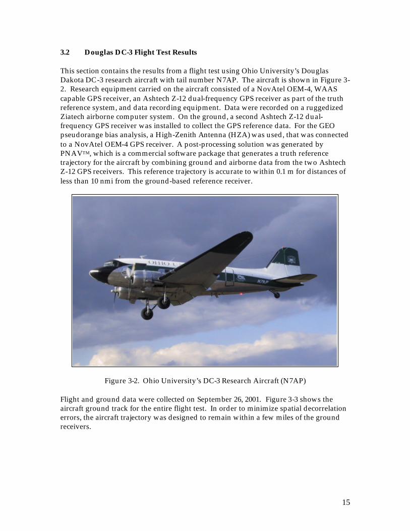
3.2 Douglas DC-3 Flight Test Results This section contains the results from a flight test using Ohio University’s Douglas Dakota DC-3 research aircraft with tail number N7AP. The aircraft is shown in Figure 3-2. Research equipment carried on the aircraft consisted of a NovAtel OEM-4, WAAS capable GPS receiver, an Ashtech Z-12 dual-frequency GPS receiver as part of the truth reference system, and data recording equipment. Data were recorded on a ruggedized Ziatech airborne computer system. On the ground, a second Ashtech Z-12 dual-frequency GPS receiver was installed to collect the GPS reference data. For the GEO pseudorange bias analysis, a High-Zenith Antenna (HZA) was used, that was connected to a NovAtel OEM-4 GPS receiver. A post-processing solution was generated by PNAVTM, which is a commercial software package that generates a truth reference trajectory for the aircraft by combining ground and airborne data from the two Ashtech Z-12 GPS receivers. This reference trajectory is accurate to within 0.1 m for distances of less than 10 nmi from the ground-based reference receiver.

Figure 3-2. Ohio University’s DC-3 Research Aircraft (N7AP)

Flight and ground data were collected on September 26, 2001. Figure 3-3 shows the aircraft ground track for the entire flight test. In order to minimize spatial decorrelation errors, the aircraft trajectory was designed to remain within a few miles of the ground receivers.

16

Figure 3-3. Aircraft Ground Track for the Flight Test on September 26, 2001

Figure 3-4 shows the satellite skyplot, which shows the azimuth and elevation angles of the satellites that were available during the flight test. The Pseudorandom Noise (PRN) numbers are indicated at the start of each satellite track. For data analysis, only satellites above a 30-degree elevation angle were used, since the High-Zenith Antenna (HZA) tracks satellites between 30 and 90 degrees in elevation. The Atlantic Ocean Region West (AOR-W) Geostationary satellite PRN is 122. PRN 122 has an elevation angle of approximately 36 degrees.

-82.3 -82.25 -82.2 -82.15 -82.1 -82.05 -82 39.1

39.15

39.2

39.25

39.3

39.35

Longitude

Latitude

17

Figure 3-4. Satellite Skyplot for the Flight Test on September 26, 2001

Ionospheric divergence is removed from the GPS satellites through the dual-frequency AD measurements. For the GEO, only the L1 frequency is available. Therefore, the GEO ionospheric divergence is removed by subtracting a parabolic fit to the CMC residuals. Figure 3-5 shows both the aircraft and ground CMC results for PRN 29.

Figure 3-5. CMC for PRN 29; Aircraft (top); Ground (bottom)

3.32 3.325 3.33 3.335 3.34 3.345

x 105

-3

-2

-1

0

1

2

3AIR: L1 Code-Carrier for SV29 OEM4 Std = 0.13127

3.32 3.325 3.33 3.335 3.34 3.345

x 105

-3

-2

-1

0

1

2

3GND: L1 Code-Carrier for SV29 Std = 0.032327

PRN 22

PRN 20

PRN 1

PRN 122

PRN 25

PRN 29

PRN 6 PRN 14

PRN 3 PRN 13

Time in seconds

18

PRN 122 CMC results are shown in Figure 3-6.

Figure 3-6. CMC for PRN 122 (AOR-W); Aircraft (top); Ground (bottom)

Table 3-1 shows the standard deviations of the CMC residuals for both the ground and aircraft measurements. Carrier smoothing with a 100-s time constant was applied to the pseudorange measurements.

Table 3-1. Standard Deviations of CMC Residuals for the DC-3 Flight Test PRN 1 PRN 20 PRN 22 PRN 25 PRN 29 PRN 122 Aircraft 0.20 m 0.13 m 0.17 m 0.13 m 0.13 m 0.22 m Ground 0.04 m 0.05 m 0.03 m 0.04 m 0.03 m 0.15 m

Due to the narrow bandwidth of 2 MHz compared to the 16-MHz bandwidth used in the GPS receiver for the GPS satellites, the thermal noise power contribution for the GEO is 8 times higher than that of the GPS satellites. This results in a higher noise level by approximately a factor of 3 for the GEO measurements. On the ground, additional noise is contributed by multipath, resulting in an overall noise level for the GEO of 0.15 m (1-sigma). The noise in the aircraft data is much larger than expected and became the subject of a detailed investigation [2]. Additional pseudorange error was found to be caused by two Very-High Frequency (VHF) antennas close to the GPS reception antenna on the DC-3, as shown in Figure 3-7.

3.32 3.325 3.33 3.335 3.34 3.345

x 105

-3

-2

-1

0

1

2

3AIR: L1 Code-Carrier for SV122 OEM4 Std = 0.22052

3.32 3.325 3.33 3.335 3.34 3.345

x 105

-3

-2

-1

0

1

2

3GND: L1 Code-Carrier for SV122 Std = 0.15295

Time in seconds

19

Figure 3-7. DC-3 Aircraft Antenna Installation

It was found that the VHF antennas have little impact on the accuracy of the accumulated Doppler measurements, but they can introduce meter-level errors on the pseudorange measurements. The mechanism for these errors is similar to antenna group delay errors discussed in Section 5.0. To verify that the pseudorange errors are dominated by the VHF antennas, a second flight test was scheduled on a smaller aircraft that does not have top-mounted VHF antennas, see Section 3.3. Next, double differences (DDs) were calculated for GPS satellite pairs as well as GPS-GEO satellite pairs. Figure 3-8 shows the DD results for PRNs 20 and 29, while Figure 3-9 shows the results for PRNs 29 and 122 (GEO).

ç GPS Antenna

ç Second VHF Antenna

ç Forward VHF Antenna

20

Figure 3-8. PR (top) and AD (bottom) Double Differences for PRNs 20 and 29

Figure 3-9. PR (top) and AD (bottom) Double Differences for PRNs 29 and 122 (GEO)

Table 3-2 summarizes the mean values of the PR DDs for selected satellites that were tracked above 30-degrees elevation angle throughout the 36-minute flight segment.

0 500 1000 1500 2000 2500-3

-2

-1

0

1

2

3Code DD SV20 vs SV29 Mean = -0.03743

Run time in s

met

ers

0 500 1000 1500 2000 2500-3

-2

-1

0

1

2

3Carrier DD SV20 vs SV29

Run time in s

met

ers

0 500 1000 1500 2000 2500-5

0

5Code DD SV29 vs SV122 Mean = 0.50479

Run time in s

met

ers

0 500 1000 1500 2000 2500-5

0

5Carrier DD SV29 vs SV122

Run time in s

met

ers

21

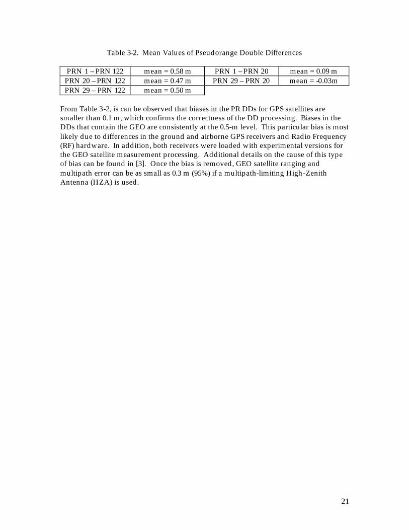
Table 3-2. Mean Values of Pseudorange Double Differences

PRN 1 – PRN 122 mean = 0.58 m PRN 1 – PRN 20 mean = 0.09 m PRN 20 – PRN 122 mean = 0.47 m PRN 29 – PRN 20 mean = -0.03m PRN 29 – PRN 122 mean = 0.50 m

From Table 3-2, is can be observed that biases in the PR DDs for GPS satellites are smaller than 0.1 m, which confirms the correctness of the DD processing. Biases in the DDs that contain the GEO are consistently at the 0.5-m level. This particular bias is most likely due to differences in the ground and airborne GPS receivers and Radio Frequency (RF) hardware. In addition, both receivers were loaded with experimental versions for the GEO satellite measurement processing. Additional details on the cause of this type of bias can be found in [3]. Once the bias is removed, GEO satellite ranging and multipath error can be as small as 0.3 m (95%) if a multipath-limiting High-Zenith Antenna (HZA) is used.

22

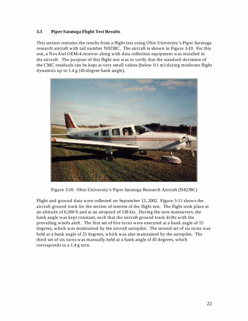
3.3 Piper Saratoga Flight Test Results This section contains the results from a flight test using Ohio University’s Piper Saratoga research aircraft with tail number N8238C. The aircraft is shown in Figure 3-10. For this test, a NovAtel OEM-4 receiver along with data collection equipment was installed in the aircraft. The purpose of this flight test was to verify that the standard deviation of the CMC residuals can be kept at very small values (below 0.1 m) during moderate flight dynamics up to 1.4 g (45-degree bank angle).

Figure 3-10. Ohio University’s Piper Saratoga Research Aircraft (N8238C)

Flight and ground data were collected on September 13, 2002. Figure 3-11 shows the aircraft ground track for the section of interest of the flight test. The flight took place at an altitude of 6,500 ft and at an airspeed of 138 kts. During the turn maneuvers, the bank angle was kept constant, such that the aircraft ground track drifts with the prevailing winds aloft. The first set of five turns were executed at a bank angle of 15 degrees, which was maintained by the aircraft autopilot. The second set of six turns was held at a bank angle of 25 degrees, which was also maintained by the autopilot. The third set of six turns was manually held at a bank angle of 45 degrees, which corresponds to a 1.4 g turn.

23

Figure 3-11. Aircraft Ground Track for the Flight Test on September 13, 2002

Figure 3-12 shows CMC residuals for PRN 25, which was at an elevation angle of approximately 76 degrees. This satellite was at the highest elevation angle, which ensures continuous tracking even when the aircraft bank angle reaches 45 degrees. The standard deviation of the smoothed CMC for PRN 25 is 0.03 m.

Figure 3-12. CMC Residuals for PRN 25 (Elevation ~76 degrees)

10 12 14 16 18 20 22 24 26 28 30-60

-58

-56

-54

-52

-50

-48

-46

-44

-42

-40Horizontal Position - Flight Segment: toga3.raw

East in km

Nor

th in

km

0

200

400 PRN 25 Aircraft Heading

Heading in degrees

-2

0

2 Raw L1 Code-Carrier OEM4 std = 0.23 m

in meters

0 5 10 15 20

25 30 35 40 -0.2

0

0.2 Smoothed (Tau = 100 s) L1 Code-Carrier OEM4 std = 0.03 m

in meters

Run Time in minutes (Start = 500300 s)

24

Figure 3-13 shows CMC residuals for PRN 14, which was at an elevation angle of approximately 45 degrees with respect to the local horizon. During the 45-degree turns, the satellite elevation angle with respect to the aircraft goes as low as 0 degrees, but the data do not show any significant errors during this portion of the flight. The standard deviation of the smoothed CMC for PRN 14 is 0.04 m.

Figure 3-13. CMC Residuals for PRN 14 (Elevation ~45 degrees)

From the results presented in figures 3-12 and 3-13 it can be concluded that the CMC residuals are at the cm-level, which confirms that airborne PR measurements can be made with accuracies better than 0.1 m.

0

200

400 PRN 14 Aircraft Heading

Heading in degrees

-2

0

2 Raw L1 Code-Carrier OEM4 std = 0.27 m

in meters

0 5 10 15 20 25

30

35

40 -0.2

0

0.2 Smoothed (Tau = 100 s) L1 Code-Carrier OEM4 std = 0.04 m

in meters

Run Time in minutes (Start = 500300 s)

25

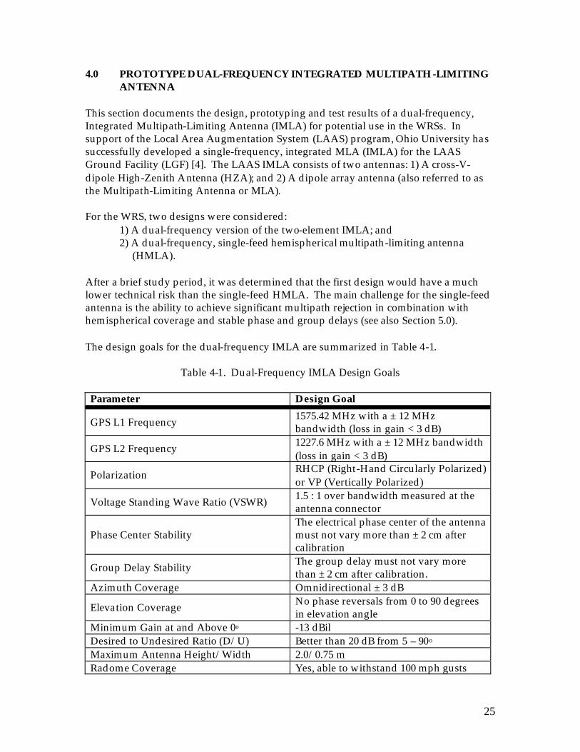
4.0 PROTOTYPE DUAL-FREQUENCY INTEGRATED MULTIPATH-LIMITING ANTENNA

This section documents the design, prototyping and test results of a dual-frequency, Integrated Multipath-Limiting Antenna (IMLA) for potential use in the WRSs. In support of the Local Area Augmentation System (LAAS) program, Ohio University has successfully developed a single-frequency, integrated MLA (IMLA) for the LAAS Ground Facility (LGF) [4]. The LAAS IMLA consists of two antennas: 1) A cross-V-dipole High-Zenith Antenna (HZA); and 2) A dipole array antenna (also referred to as the Multipath-Limiting Antenna or MLA). For the WRS, two designs were considered:

1) A dual-frequency version of the two-element IMLA; and 2) A dual-frequency, single-feed hemispherical multipath-limiting antenna

(HMLA). After a brief study period, it was determined that the first design would have a much lower technical risk than the single-feed HMLA. The main challenge for the single-feed antenna is the ability to achieve significant multipath rejection in combination with hemispherical coverage and stable phase and group delays (see also Section 5.0). The design goals for the dual-frequency IMLA are summarized in Table 4-1.

Table 4-1. Dual-Frequency IMLA Design Goals Parameter Design Goal

GPS L1 Frequency 1575.42 MHz with a ± 12 MHz bandwidth (loss in gain < 3 dB)

GPS L2 Frequency 1227.6 MHz with a ± 12 MHz bandwidth (loss in gain < 3 dB)

Polarization RHCP (Right-Hand Circularly Polarized) or VP (Vertically Polarized)

Voltage Standing Wave Ratio (VSWR) 1.5 : 1 over bandwidth measured at the antenna connector

Phase Center Stability The electrical phase center of the antenna must not vary more than ± 2 cm after calibration

Group Delay Stability The group delay must not vary more than ± 2 cm after calibration.

Azimuth Coverage Omnidirectional ± 3 dB

Elevation Coverage No phase reversals from 0 to 90 degrees in elevation angle

Minimum Gain at and Above 0o -13 dBil Desired to Undesired Ratio (D/U) Better than 20 dB from 5 – 90o Maximum Antenna Height/Width 2.0/0.75 m Radome Coverage Yes, able to withstand 100 mph gusts

26

It is noted that for L1 both pseudorange (PR) and accumulated Doppler (AD) measurements are important, while for L2, the primary emphasis is on AD measurement performance. L1 PR measurements are the basis for the differential correction generation, while AD measurements on L1 and L2 are used for ionospheric corrections as well as for the CNMP algorithm (see Section 2.0). A key design parameter for the antenna is the Desired–to-Undesired Ratio (D/U), which is the gain ratio between opposite elevation angles. The D/U provides the ratio of the direct (desired) to the multipath (undesired) signal considering a flat ground plane below the antenna. If no other obstacles are present, then the D/U is sufficient to characterize the performance of the installed antenna. If the D/U is better than 20 dB, PR multipath errors due to ground reflections will be less than 1.5 m. In practice, multipath errors will be much smaller than 1.5 m, as the height above ground of the antenna can also be limited. For example, if the height above ground is less than 1 m, then the ground-induced multipath error will be less than 0.2 m. AD errors are limited to approximately 3 mm for D/U better than 20 dB. Sections 4.1 and 4.2 describe the design and performance of the dual-frequency HZA and MLA, respectively. Efforts to further the development and field testing of the dual frequency IMLA are continuing under a separate Aviation Research Co-Operative Agreement 98-G-023.

27

4.1 Dual-Frequency High-Zenith Antenna (HZA) The dual-frequency HZA implements a combination of antenna technologies including [4]:

a) A flat, conductive, reflecting counterpoise oriented orthogonal to the vertical axis of the antenna;

b) A shaped concave reflector electrically connected to the counterpoise, which electrically and mechanically connects to a Cross-V-Dipole element;

c) A vertically oriented, quarter wave, Radio Frequency (RF) choke which aids in the suppression of the surface wave which exists on the surface of the microwave absorbing material; and

d) A beam-forming shaped piece of RF absorbing material with a precisely known and controlled carbon fill factor. This “Shaped Absorber” provides controlled positive angle radiation through use of its shaped inside contour as well as a shaped outside contour to control the broadside and negative angle portions of the radiation pattern.

The HZA is enclosed in a fiberglass radome with associated aluminum plate/hub for mounting and environmental protection. The HZA is shown in Figure 4-1 without the fiberglass radome. The HZA has an integral Low Noise Amplifier (LNA) used to amplify low level GPS signals and a 90º power hybrid combiner (for the Cross-V-Dipole Feed) which is connected to combine the Cross-V-Dipoles in the RHCP sense. The symmetrical Cross-V-Dipole radiating element helps maintain close to equal vertically and horizontally polarized RHCP orthogonal components. The Cross-V-Dipole exhibits a very stable and accurate phase center as well a minimal group delay due to its electrical symmetry and large operational bandwidth. Since the HZA was designed for a large bandwidth, it was determined that a recent version of this antenna would be sufficient to receive both the L1 and L2 frequencies. Therefore, modifications to the antenna consisted of a change in the pre-filter to enable reception of both L1 and L2 GPS signals. Figure 4-2 shows the D/U ratios for both the L1 and L2 frequencies. From this figure, it is found that the HZA meets the D/U design goal of 20 dB or better.

28

Figure 4-1. Dual-Frequency High-Zenith Antenna (from [4])

Figure 4-2. High-Zenith Antenna D/U Performance at L1 (red, top curve), L2 (blue,

middle curve), and Design Goal (black, constant line at 20 dB)

é Top-view showing the Cross-V-Dipole antenna. ç Side-view showing the RF absorber and combiner/amplifier network.

120 140 160 180 200 220 240 0

5

10

15

20

25

30

35

40

45

50 Measured D/U: L1 (red) L2 (blue) Design Goal (black)

Elevation Angle (zenith = 180o)

D/U (dB)

29

4.2 Dual-Frequency Dipole Array Multipath-Limiting Antenna (MLA) The design of the dual-frequency dipole array antenna was significantly more complex than that of the HZA. Initial design trade-offs were completed in September of 2001. The procurement for the fabrication of the antenna was awarded in October of 2001. dB-Systems, Inc. delivered the first prototype dual-frequency MLA to Ohio University in February of 2002. Initial testing revealed the need for design iterations to enable detailed testing of the array in an indoor antenna range. After two design iterations, the modified antenna was delivered to Ohio University in May of 2003. At this point, the L2 performance had been improved and the L1 and L2 outputs were separated to enable testing of L1 and L2 individually. In order to maximize the gain at L2, the same dipole array elements were used for both L1 and L2. The MLA array consists of 14 cylindrical, vertically stacked, co-linear, dipole elements [4]. Inter-element coupling of vertically polarized, co-linear dipoles is small, which aids in the forming and maintaining of a precisely controlled vertical pattern. Also, the broadband response of the large diameter cylindrical dipoles provides an antenna array which exhibits very large bandwidth. This large bandwidth yields minimal group delay variation over the operational frequency band. The group delay is also maintained as a function of azimuth due to the constant phase and bandwidth symmetry of the dipole element. This azimuth pattern phase symmetry provides phase variations of less than 10 electrical degrees over a typical 360º azimuth pattern. A close-up of five dipole array elements is shown in Figure 4-3. Also shown in this figure are the feeds that connect to each of the elements in four points, separated by 90 degrees in azimuth. When the L2 feeds are also connected, each element is fed by a total of eight connections. The L1 and L2 feeds are combined in separate distribution networks. The outputs of the L1 and L2 distribution networks are combined in a single combiner, which is connected to a wide-band, low-noise amplifier.

Figure 4-3. Dipole Array Elements (from [4])

30

The D/U performance for both the L1 and L2 frequencies is shown in Figure 4-4. From this figure, it is found that the MLA meets the D/U design goal of 20 dB or better.

Figure 4-4. Dipole Array MLA D/U Performance at L1 (red, top curve), L2 (blue,

middle curve), and Design Goal (black, constant line at 20 dB)

0 5 10 15 20 25 30 35 40 0

5

10

15

20

25

30

35

40

45

50 Measured D/U: L1 (red) L2 (blue) Design Goal (black)

Elevation Angle in degrees

D/U (dB)

31

5.0 GPS ANTENNA PHASE AND GROUP DELAYS The term antenna phase center and antenna phase center corrections are in widespread use in the GPS community [5-7]. The intent of a phase center correction is to compensate for the difference between the actual “point” where the satellite signals enter the antenna and a fixed reference point on the antenna. Phase center corrections are usually provided as a function of elevation angle [7], and can only be used to correct the GPS receiver Accumulated Doppler (AD) measurements. According to the International Institute of Electrical and Electronics Engineers (IEEE), the term phase center is defined as [6, 8]:

“The location of a point associated with an antenna such that, if it is taken as the center of a sphere whose radius extends into the far-field, the phase of a given field component over the surface of the radiation sphere is essentially constant, at least over that portion of the surface where the radiation is significant. Note: Some antennas do not have a unique phase center.”

According to this definition, the term phase center is only appropriate if the location of the phase center is constant and unique. For antennas that exhibit phase variations as a function of elevation and/or azimuth angles, it is seldom possible to solve for the antenna phase center, or centers, as defined above. Furthermore, if the antenna phase response is a function of frequency, then group delay variations that affect the pseudorange (PR) measurements also become significant. To compensate for both phase and group delay variations as a function of elevation and azimuth angles, a new methodology to calibrate and correct PR and AD measurements is introduced in this section. In general, antennas exhibit unequal phase and group delays. The phase delay in seconds is given by:

[s] )(

)(phase ωωφ

=ωτ (5-1)

Accumulated Doppler (AD) measurements represent continuous wave (CW) measurements, and are therefore subjected to the antenna phase delay. The group delay is a measure of the time delay that is experienced by a narrow-band signal packet. If the group delay is constant over the GPS signal bandwidth, then the pseudorange measurements are subjected to the antenna group delay, which is given by:

[s] d

)(d)(group ω

ωφ=ωτ (5-2)

Both phase and group delays can be expressed in terms of meters through multiplication by the speed of light:

32

[m] d

)(dc)( and ,

)(c)( groupphase ω

ωφ=ωτ

ωωφ

=ωτ (5-3)

If the phase is not a function of frequency, or φ(ω1) = φ(ω2), then the numerator of the group delay equation, dφ(ω), is zero, which means that the group delay is zero. In other words, if the change in phase is not a function of frequency, then the group delay is zero. A circularly-polarized antenna has a phase pattern that is a function of azimuth angle. The measured phase will increase by exactly 360 degrees for each 360-degree rotation in azimuth angle ψ(t). The phase added to the AD measurement as a function of azimuth angle in radians is given by:

[rad] )t()t(rotation ψ=φ (5-4) Since the phase increase is the same for all frequencies, the group delay is zero. This causes the GPS AD and PR measurements to become non-coherent. The phase increase is caused by:

1. Antenna rotation that occurs when the vehicle to which the antenna is mounted changes heading;

2. Rotation of the satellite around a stationary antenna due to the satellite orbit. The first rotation is common to all satellites and; therefore, mostly affects the clock solution of the GPS receiver. The second rotation is different for each satellite and therefore must be corrected for high-accuracy, stand-alone applications. In differential applications, this rotation is common to the reference and user antennas. Note that for a linearly-polarized antenna, such as the dipole array multipath-limiting antenna (MLA), the antenna phase pattern is the same for all azimuth directions. As a result, the measurements from the MLA must be adjusted by adding in the rotation correction to avoid differential errors, since the user antenna is circularly-polarized.

33

5.1 Antenna Calibration Requirements This section details the information that is required to correct GPS antenna phase and group delays. The methodology used to determine the calibration curves for phase and group delays must consider the following:

a) Single frequency calibration: The calibration technique should be valid for single frequency antennas, such as those used in the Local Area Augmentation System (LAAS) Ground Facility (LGF).

b) Calibration must be a function of elevation and azimuth angles. c) Corrections must be made for phase and group delays: Group delay corrections

imply that measurements are taken at multiple frequencies surrounding the L1 and L2 frequencies.

d) The corrections must provide an absolute reference with respect to the Aperture Reference Point (ARP). The ARP is related to the antenna mount, such that the ARP can be surveyed before the antenna is installed. Also, it is important that dual frequency antennas are calibrated separately at L1 and L2, such that absolute corrections are available for both the L1 and L2 frequencies.

e) Phase delay calibration must be accurate to within a few mm: This level of accuracy is required for survey-type applications and for satellite monitoring applications.

f) Group delay calibration must be accurate to within 1 cm: This level of accuracy is required to limit deterministic bias errors to a few cm. This is of particular importance for the LAAS integrity design [9].

g) To evaluate and model installed antenna performance, antenna polarization and multipath desired-to-undesired ratio (D/U) are also needed: Antenna polarization may affect the phase and/or group delay corrections. The D/U is important for the evaluation of field data with respect to phase and group delays.

34

5.2 Importance of Group Delays for WAAS and LAAS Both the Local-Area Augmentation System (LAAS) and the Wide-Area Augmentation System (WAAS) use Pseudorange-based differential corrections. In the LAAS, the smoothing time constant of the PR measurements is set at 100 s. Therefore, as long as the phase delay correction correlation time is much larger than 100 s, the effect on the differential corrections is negligible, and the group delay variations dominate the accuracy of the differential corrections. Figure 5-1 illustrates the limited effect that an uncorrected phase delay has on the accuracy of the smoothed PR. Even though the phase delay varies from 0 to 0.7 m, the smoothed PR error is less than 2 cm, which is not visible due to the PR noise level.

Figure 5-1. Example of LAAS Smoothed Pseudorange in the Presence of Phase Delays

For WAAS, both phase and group delay corrections are important since the smoothing time constant for the PR measurements can be much longer than 100 s. Furthermore, both L1 and L2 accumulated Doppler (AD) measurements are used to reduce the PR correction error (see Section 2.0).

0 1000 2000 3000 4000 5000 6000 7000 8000 -5

0

5 Raw Pseudorange in m

0 1000 2000 3000 4000 5000 6000 7000 8000 -1 -0.5

0 0.5

1 Phase Delay in m

0 1000 2000 3000 4000 5000 6000 7000 8000 -1 -0.5

0 0.5

1 Smoothed Pseudorange in m

Time in seconds

35

5.3 Measurement of Antenna Group Delay Several methods are available to measure antenna group delays, including:

1) Indoor or outdoor antenna range measurements at multiple frequencies 2) Indoor or outdoor measurements using a GPS signal generator 3) Absolute outdoor measurements using GPS satellite signals 4) Relative outdoor measurements using GPS satellite signals and a reference

antenna The first method is the most straightforward method to measure antenna group delays, since it enables the isolation of antenna group delay from other error sources, such as GPS receiver thermal noise and multipath. Since the other three methods rely on the GPS signal itself, it is not easily possible to separate the group delay from other error sources. Furthermore, antenna range measurements provide group delays for different signal polarizations, true gain patterns, and ground multipath D/U ratios. 5.3.1 Sensitivity of antenna range group delay to phase measurement noise To measure group delays using an antenna range, the following approximation is used:

f4)()(

c2

)()(c

d)(d

c)(group ∆πω∆−ωφ−ω∆+ωφ

=ω∆

ω∆−ωφ−ω∆+ωφ≈

ωωφ

=ωτ (5-5)

For GPS, 2∆f can be set to the signal bandwidth of 20 MHz, such that the group delay is approximated by:

( ))MHz 42.1565(2 and )MHz 42.1585(2 :where

[m] )()(15)(

12

121Lgroup

π=ωπ=ω

ωφ−ωφ≈ωτ (5-6)

To calculate the group delay with noise levels below 1 cm (1 sigma), the required phase measurement noise is given by (assuming that the noise on the two phase measurements is independent):

o)1Lgroup()1()2( 027.0

215180

=σπ

=σ=σ ωτωφωφ (5-7)

Therefore, the antenna range phase noise and stability must be better than 0.027O (1-sigma) in order to measure group delays with 1-sigma noise levels below 1 cm. 5.3.2 Comparison of antenna range and CMC-derived group delays If outdoor measurements using GPS satellite signals are used, then code-minus-carrier (CMC) processing is the most direct method to calculate antenna group delays. Once the antenna phase delays are known, then the difference between phase and group

36

delays would also be contained in the CMC residual. If antenna range and CMC residuals are compared, the following differences must be taken into account:

1. Chamber phase noise: Group delay noise should be kept below 1 cm (1-sigma); 2. GPS receiver thermal noise: Typically on the order of 5-10 cm (1-sigma) for a 100-

s smoothing time constant; 3. GPS receiver errors: Typically less than a few cm (see Section 3.3), but care must

be taken to verify and confirm that the GPS receiver is functioning at this level of performance;

4. Antenna range survey error: Precise survey of the rotation center of the antenna under test relative to the Aperture Reference Point (ARP) must be maintained at the mm-level;

5. Mean values are reduced in the CMC processing: The average value for each corrected CMC is subtracted (see Section 2.0 and below);

6. Satellite antenna phase and group delays: If the satellite phase and group delays are not equal, then the difference will be contained in the CMC residuals. The exact size of this error is not known at this time, but it should be at the cm-level based on CMC observations for small reception antennas;

7. Multipath: Three types of multipath should be considered: a. Ground multipath, which is significant for antennas with D/U below 10

dB resulting in multipath errors on the order of several meters. Mitigating factors are the ability to model ground multipath based on the antenna multipath D/U, gain pattern, polarization, and installation geometry. Also, the multipath fading frequency as a function of elevation angle is typically much larger than the group delay variation as a function of elevation angle;

b. Hardware multipath: For example, a cable with mismatched impedances at both ends can introduce hardware errors that are not equal for different satellites [10]. This type of error can be kept well below 1 cm for most installations;

c. Near-field effects: For large antenna apertures with significant gain to the ground or nearby obstacles, multipath reflections/diffractions may not be accurately modeled as plane waves. Although near-field effects have not been found to be significant to date, it should be an area for future investigations.

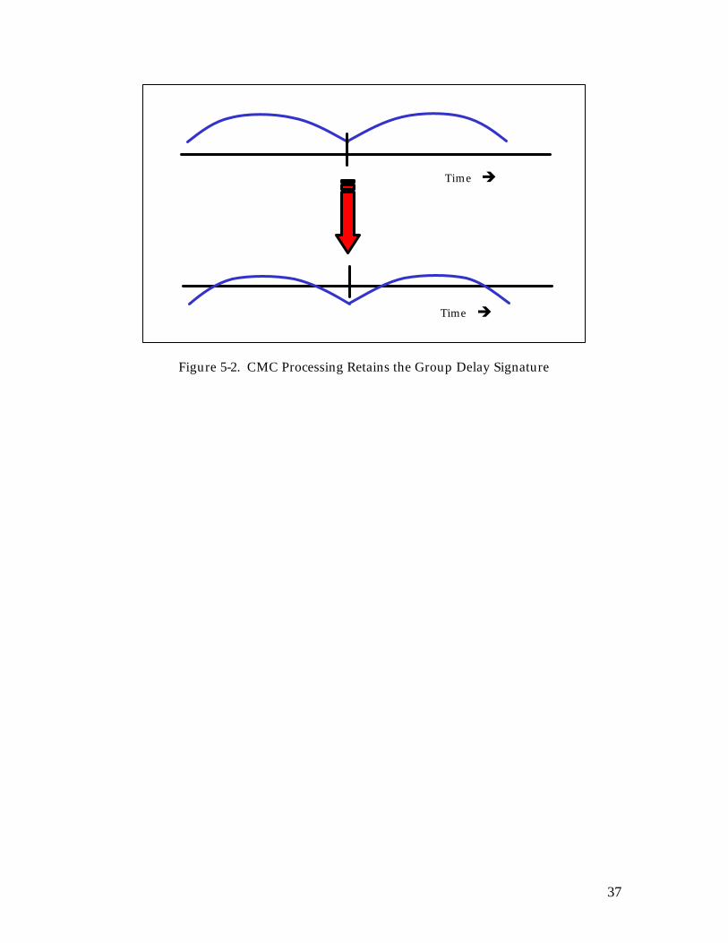
Item 5, mean value reduction in CMC processing, is further illustrated in Figure 5-2. Although the average bias is removed for each satellite track, the CMC residual still retains the signature of antenna group delay variations once the CMC is corrected for antenna phase delay variations. In the CMC processing, it is therefore important that satellite tracks are taken over entire satellite passes to avoid passes that remove the group delay signature.

37

Figure 5-2. CMC Processing Retains the Group Delay Signature

Time è

Time è

38

5.4 Calibration Methodology To obtain phase and group delay calibration curves as a function of elevation and azimuth angles, the following procedure is followed [11]:

1. Obtain antenna range measurements as a function of elevation and azimuth angles at multiple frequencies surrounding the L1 (and L2) frequency band. Collect both phase and amplitude responses for horizontal and vertical polarizations.

2. From the antenna range measurements derive antenna gain curves, D/U curves, and calculate both phase and group delay calibration curves for different polarizations with respect to the Aperture Reference Point (ARP).

3. Collect field data to verify that no other significant error sources are present (see Section 5.3)

4. Process the field data using the following observables: Code-minus-Carrier (CMC), and double difference processing of accumulated Doppler (AD) measurements against a survey antenna.

5. Comparison of antenna range and field data results for consistency. On the antenna range, the antenna is usually not rotated around the ARP, such that a correction is required to translate the measurements to the ARP. Consider the geometry depicted in Figure 5-3.

Figure 5-3. Antenna Range Measurement Geometry

Consider that the antenna has a fixed phase center located at a distance, d, above the antenna rotation point. It is also given that the antenna is rotated at a distance, drot,

Phase Measurement

φmeas ARP

θel

d ∆φ

drot

ç Antenna under test

39

above the ARP. The phase measurement as a function of elevation angle at a fixed azimuth angle is then given by:

λπ

=

θ+ψφ=ψθφ2k :where

)sin()d(k)(),( elref0refelmeas (5-8)

The initial phase, φ0, represents a constant phase due to measurement equipment, cables, free space propagation and propagation within the antenna. The initial phase for a particular azimuth angle can be measured by setting the elevation angle to zero degrees. Note that when the phase center is above the rotation point, the phase center will move toward the wave front as the elevation angle increases, which causes an increase in the measured phase (positive Doppler frequency as the phase center moves closer to the radiation source). The measured phase is translated to the ARP using the following equation:

)sin()d(k)(),(),( elrot0elmeaselARP θ+ψφ−ψθφ=ψθφ (5-9) Group delay calibration curves are derived from the phase calibration curves obtained at different frequencies as given by Equation (5-5). If the phase center location is not constant, then an additional phase term will be measured as a function of elevation angle. Also, it is possible that the measured phase is a function of azimuth angle. One method to obtain the phase and group delay calibration curves is to measure all elevation angles from 0 to 360 degrees for several azimuth angles (e.g. 0, 45, 90, and 135 degrees). For each full elevation rotation, two azimuth angles are obtained: ψ and ψ+180O. Next, two options are available:

1. Adjust each azimuth cut by a constant phase to match the measured phase for the reference azimuth at an elevation angle of 90 degrees; or

2. Measure the phase as a function of all azimuth angles for a constant elevation angle of zero degrees and use this response to find the initial phase for each azimuth angle with respect to the reference azimuth.

The second method always provides absolute phase and group delay corrections, but requires a precise measurement cut at zero-degree elevation. For antennas with an “undefined” pattern at 90-degree elevation (e.g. a vertically-polarized dipole-array antenna), this is the only practical method to obtain calibration curves that are a function of both elevation and azimuth angles. For antennas that have a good pattern behavior at 90-degree elevation (e.g. HZA or most survey-quality antennas), the first method is often easier to use, since it does not require the additional azimuth cut.

40

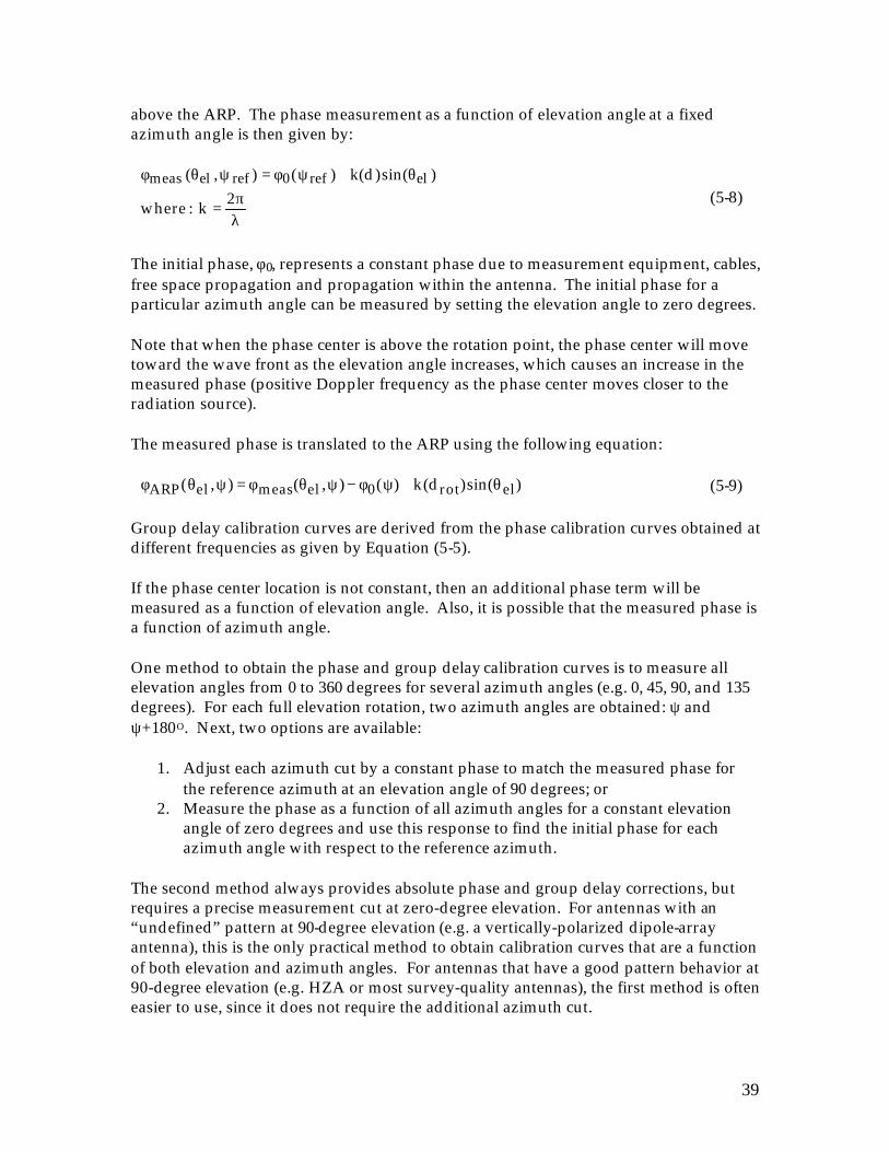
5.5 Compact Antenna Range Measurements One antenna range that is capable of providing the required measurements for the antenna phase and group calibration curves is the Compact Radar Measurement Range at Ohio State University’s ElectroScience Laboratory (ESL). Figure 5-4 shows a picture of the antenna range.

Figure 5-4. Compact Radar Measurement Range

Key features of this antenna range are as follows. The large reflector is used to create far-field conditions at the location of the antenna under test. The edges of the reflector are rolled, which provides a test area for 8-ft targets. The transmitter is pulsed and the receiver is gated, which eliminates multipath errors from the building structure. Furthermore, radar absorbing materials are mounted on the inside of the range to efficiently dissipate unwanted energy and standing wave reflections. The resulting measurement phase noise is on the order of 0.01O.

Electro-Science Laboratory The Ohio State University

Antenna under test

Rolled-Edge Reflector

Transmit Horn

Antenna

Antenna support structure and computer-controlled

turn-table

41

5.6 Case Study: High-Zenith Antenna Calibration This section provides preliminary data for a prototype High-Zenith Antenna (HZA) as described in Section 4.1 [11]. Figure 5-5 shows a picture of the antenna as mounted on the Compact Radar Measurement Range. The measurement geometry is depicted in Figure 5-6. Two azimuth cuts were taken to obtain antenna azimuth performance in the four cardinal directions.

Figure 5-5. High-Zenith Antenna on the Compact Radar Measurement Range

Figure 5-6. Compact Range Measurement Geometry

360o rotation in elevation angle

Two azimuth cuts (rotate antenna by 90o)

TOP VIEW

42

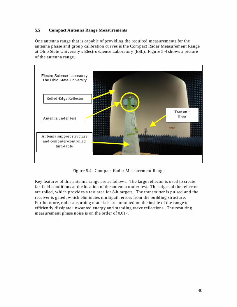
To verify the ground multipath rejection performance, the multipath D/U was calculated and is shown in Figure 5-7. Also shown in this figure is the D/U performance for the NovAtel PinWheel antenna. Note that even though the D/U performance for the HZA is better than 20 dB at low-elevation angles, the gain of the HZA is much lower than that of the PinWheel antenna at elevation angles below 30 degrees. Because of this, the HZA is not used for elevation angles below 30 degrees.

Figure 5-7. Ground Multipath D/U for High Zenith and PinWheel Antennas

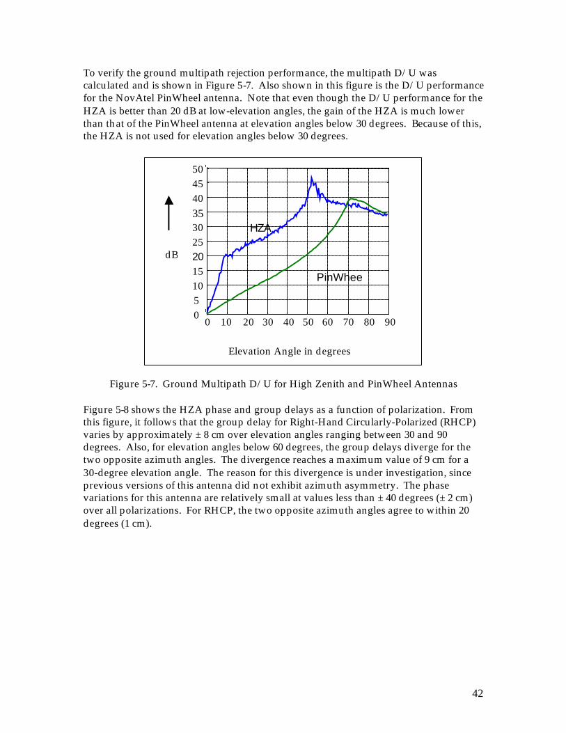
Figure 5-8 shows the HZA phase and group delays as a function of polarization. From this figure, it follows that the group delay for Right-Hand Circularly-Polarized (RHCP) varies by approximately ± 8 cm over elevation angles ranging between 30 and 90 degrees. Also, for elevation angles below 60 degrees, the group delays diverge for the two opposite azimuth angles. The divergence reaches a maximum value of 9 cm for a 30-degree elevation angle. The reason for this divergence is under investigation, since previous versions of this antenna did not exhibit azimuth asymmetry. The phase variations for this antenna are relatively small at values less than ± 40 degrees (± 2 cm) over all polarizations. For RHCP, the two opposite azimuth angles agree to within 20 degrees (1 cm).

0 10 20 30 40 50 60 70 80 90 0 5 10 15 20 25 30 35 40 45 50

dB

Elevation Angle in degrees

PinWheel

HZA

43

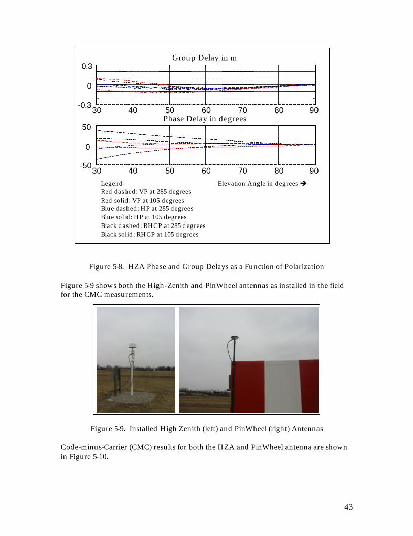
Figure 5-8. HZA Phase and Group Delays as a Function of Polarization Figure 5-9 shows both the High-Zenith and PinWheel antennas as installed in the field for the CMC measurements.

Figure 5-9. Installed High Zenith (left) and PinWheel (right) Antennas

Code-minus-Carrier (CMC) results for both the HZA and PinWheel antenna are shown in Figure 5-10.

-0.3 30 40 50 60 70 80 90

0

0.3

30 40 50 60 70 80 90 -50

0

50

Group Delay in m

Phase Delay in degrees

Elevation Angle in degrees è Legend: Red dashed: VP at 285 degrees Red solid: VP at 105 degrees Blue dashed: HP at 285 degrees Blue solid: HP at 105 degrees Black dashed: RHCP at 285 degrees Black solid: RHCP at 105 degrees

44

Figure 5-10. CMC Results for High-Zenith and PinWheel Antennas

The CMC results for the PinWheel antenna shown on the right-hand side of Figure 5-10 verify the CMC processing and its ability to measure differences between phase and group delays at the cm-level. The CMC results for the HZA show less noise than that obtained for the PinWheel antenna, which was expected due to its better D/U performance in combination with sufficient gain for elevation angles above 30 degrees. The lower plots show the CMC binned and averaged by elevation angle bins of 1-degree each. The HZA shows a variation that is within ± 8 cm. This level of variation is similar to the antenna range data. The actual values, however, are not in agreement for the different elevation angles. The reason for this is under investigation, but several mechanisms for disagreement between antenna range and CMC results were identified in Section 5.3.2. Currently, the most likely reason is that the antenna was not precisely surveyed when it was rotated inside the antenna range. It can be concluded from this case study that the proposed calibration method is feasible based on the results of the antenna range and field data results. The performance of this method is consistent with the calibration requirements listed in Section 5.1.

30 40 50 60 70 80 90 Elevation angle in degrees

-0.5

-0.3

-0.1 0

0.1

0.3

0.5

30 40 50 60 70 80 90 Elevation angle in degrees

CMC for HZA in m (raw) CMC for PinWheel in m (raw)

Binned by elevation angle Binned by elevation angle

-0.5

-0.3

-0.1 0

0.1

0.3

0.5

-0.5

-0.3

-0.1 0

0.1

0.3

0.5 -0.5

-0.3

-0.1 0

0.1

0.3

0.5

45

6.0 SUMMARY OF RESEARCH RESULTS Major findings of the research are summarized below: 1) A dual-frequency Code Noise and MultiPath (CNMP) monitor was developed to

significantly reduce multipath error at the WAAS Reference Sites (WRS). 2) Based on ground and flight test evaluations, Narrow-Band Geostationary Satellite

(GEO) multipath and noise ranging errors can be as small as 0.3 m (95%) if a multipath-limiting High-Zenith Antenna (HZA) is used.

3) A dual-frequency Integrated Multipath-Limiting Antenna (IMLA) was prototyped and determined to be feasible for WAAS applications.

4) A new method was developed for the measurement and evaluation of GPS antenna phase and group delays.

46

7.0 REFERENCES 1. Shallberg, K., Shloss, P., Altshuler, E. and L. Tahmazyan, “WAAS Measurement

Processing, Reducing the Effects of Multipath,” Proceedings of the 14th International Technical Meeting of the Satellite Division of The Institute of Navigation, September 2001, Salt Lake City, Utah.

2. Skidmore, T. A., van Graas, F. and L. Marti, “Characterization of the DC-3 In-Flight GPS Antenna Performance,” Proceedings of the 16th International Technical Meeting of the Satellite Division of The Institute of Navigation, September 2003, Portland, Oregon.

3. Phelts, R.E., Walter, T., Akos, D., Enge P., Shallberg, K. and T. Morrissey, “Range Biases on the WAAS Geostationary Satellites,” Proceedings of the Institute of Navigation National Technical Meeting, January 2004, San Diego, CA.

4. Thornberg, D. B., Thornberg, D. S., DiBenedetto, M. F., Braasch, M. S., van Graas, F. and C. Bartone, “LAAS Integrated Multipath-Limiting Antenna,” Navigation: Journal of The Institute of Navigation, Vol. 50, No. 2, 2003.

5. Wübbena, G. and M. Schmitz, “Automated Absolute Field Calibration of GPS Antennas in Real-Time,” Proceedings of the 13th International Technical Meeting of the Satellite Division of The Institute of Navigation, September 2000, Salt Lake City, Utah.

6. Lopez, A. R., “Calibration of LAAS Reference Antennas,” Proceedings of the 14th International Technical Meeting of the Satellite Division of The Institute of Navigation, September 2001, Salt Lake City, Utah.

7. Mader, G. L., “GPS Antenna Calibration at the National Geodetic Survey,” GPS Solutions, Vol. 3, No. 1, 1999.

8. IEEE Standard 100-1996, “The IEEE Standard Dictionary of Electrical and Electronics Terms,” sixth edition, 1996.

9. Sayim, I. and B. Pervan, “LAAS Ranging Error Overbound for Non-Zero Mean and Non-Gaussian Multipath Error Distributions, Proceedings of the Annual Meeting of The Institute of Navigation, June 2003, Albuquerque, New Mexico.

10. Keith. J. P., “Multipath Errors Induced by Electronic Components in Receiver Hardware,” Proceedings of National Technical Meeting of The Institute of Navigation, January 2000, San Diego, CA.

11. Van Graas, F., Bartone, C. and T. Arthur, “GPS Antenna Phase and Group Delay Corrections,” Proceedings of the Institute of Navigation National Technical Meeting, 26-28 January 2004, San Diego, CA.