Wild-Bootstrapped Variance Ratio Test for Autocorrelation in the

Munich Personal RePEc Archive

Wild-Bootstrapped Variance Ratio Test

for Autocorrelation in the Presence of

Heteroskedasticity

Jeong, Jinook and Kang, Byunguk

Yonsei University

December 2006

Online at https://mpra.ub.uni-muenchen.de/9791/

MPRA Paper No. 9791, posted 04 Aug 2008 05:56 UTC

1

Wild-Bootstrapped Variance Ratio Test for

Autocorrelation in the Presence of Heteroskedasticity

by

Jinook Jeong1

School of Economics

Yonsei University

and

Byunguk Kang

School of Economics

Yonsei University

April 2008

Abstract

The Breusch-Godfrey’s LM test is one of the most popular tests for

autocorrelation. However, it has been shown that the LM test may be erroneous when

there exist heteroskedastic errors in regression model. Some remedies recently have

been proposed by Godfrey and Tremayne (2005) and Shim et al. (2006). This paper

suggests wild-bootstrapped variance ratio test for autocorrelation in the presence of

heteroskedasticity. We show through a Monte Carlo simulation that our wild-

bootstrapped VR test has better small sample properties and is robust to the structure of

heteroskedasticity.

Keywords: variance-ratio test, Breusch-Godfrey’s LM test, autocorrelation,

heteroskedasticity, wild bootstrap

JEL classifications: C12, C15

Acknowledgement: We are grateful for the helpful comments from Tae H. Kim, Dong

H. Kim and the participants of NAIS conference at Yonsei University. The authors are

members of ‘Brain Korea 21’ Research Group of Yonsei University.

1 Corresponding author: Professor Jinook Jeong, School of Economics, Yonsei University,

Seoul, Korea; Tel.: +82-2-2123-2493; e-mail address: [email protected]

2

I. Introduction

Breusch-Godfrey’s LM test (B-G LM test hereafter) is one of the most popular

tests for autocorrelation in regression models, as it is simple and is unrestricted by the

dynamics of error term.2 Recently, it has been shown that B-G LM test may be

misleading in the presence of variance break. Hyun et al. (2006) present a Monte

Carlo result where the empirical size of B-G LM test is distorted with a variance break.

Shim et al. (2006) propose a modified LM test and a modified variance-ratio (VR) test

to remedy B-G LM test in the presence of a variance break. However, the remedies by

Shim et al. (2006) are not free of limitations. First, their modified LM test would not

be valid with a more general form of heteroskedasticity but a variance break. For

example, a multiplicative heteroskedasticity, which is a more practical structure of

heteroskedasticity, may not be properly dealt with by their modified LM test. For

another example, their modified LM test may not be valid with ‘multiple’ variance

breaks. Second, the finite sample properties of the tests suggested by Shim et al.

(2006) may not be as good as the asymptotic properties, as the test statistics are

basically two-step estimators. Since the first-stage estimates are error-ridden, the

second-stage estimates could suffer from the cumulative errors.

We suggest a refined VR test using wild bootstrap as the remedy for various

types of heteroskedasticity. Wild bootstrap has been originally suggested by Härdle

and Mammen (1990) and been widely used to deal with heteroskedasticity.3 For

example, Godfrey and Tremayne (2005) apply wild bootstrap for B-G LM test under

heteroskedasticity. They show the empirical size and power of B-G LM test are

improved with wild bootstrap. One interesting feature of their method is the use of

2 Breusch (1978) and Godfrey (1978)

3 For example, see Mammen (1993), Davidson and Flachaire (2001), and Flachaire (2003)

among others.

3

heteroskedasticity-consistent covariance estimates in computing the LM statistic.

They first correct the covariance for heteroskedasticity and then apply wild bootstrap to

the heteroskedasticity-corrected LM statistic. We will show that wild bootstrap of our

VR test statistic does not need such pre-correction. Without using heteroskedasticity-

consistent covariance estimates, our wild-bootstrapped VR test has better power than

Godfrey-Tremayne’s LM test in finite samples. We also show through Monte Carlo

simulations that our wild-bootstrapped VR test is accurate in the presence of general

form of heteroskedasticity, and its finite sample property is significantly better than

previously proposed tests even in the presence of a variance break.

II. Model

We consider the following linear regression model:

, 1, 2,...,t t t

y X u t Tβ′= + = (1)

where t

X is 1k × vector, ( ) 0t

E u = and ( ) 0t s

E u u = for t s≠ . Our concern is

whether t

u is serially independent. The standard LM test by Breusch and Pagan

works well for the autocorrelation test if t

u is homoskedastic. However, the standard

B-G LM test may not be valid if t

u is not homoskedastic. Hyun et al. (2006)

consider a variance break case as follows.

t t tu σ η= (2)

2 2 2

1 21[ ] 1[ ]t t T t Tσ σ τ σ τ= ≤ + >

where t

η is (0,1)IID and break timing, τ is between 0 and 1. In this model,

variance of t

u , 2

tσ is given by 2

1σ for t Tτ≤ and changes into 2

2σ after Tτ .

Hyun et al. (2006) report that the empirical size of B-G LM test is distorted and that the

magnitude of distortion depends on the degree of break, break timing, and the lag length

(p) of the error term.

4

For this problem with variance break, Shim et al. (2006) suggest two tests, the

modified LM test based on feasible generalized least squares (FGLS) and the modified

variance-ratio (VR) test. The FGLS-based LM test procedure is as follows.

i) Estimate the break point by quasi-maximum likelihood estimation by Bai et

al. (1998) or the least squares method by Bai (1993).

ii) According to the estimated break, estimate σ1 and σ2 from the subsamples.

iii) Using the estimated variances, apply FGLS to estimate the FGLS residuals.

iv) Compute the LM statistic using the FGLS residuals, and apply the

asymptotic χ2(p) distribution for the test.

It is noted that the FGLS-based LM test is not robust to the structure of

heteroskedasticity. If the number of break points is not known a priori, or if other

forms of heteroskedasticity than variance break exist in the data, the FGLS-based LM

test would be invalid.

On the other hand, the modified VR test employs the VR test by Lo and

MacKinley (1988, 1989). The VR test is originally designed for serial correlation in a

time series variable. It examines if the variance of ‘q-period return’ is exactly q times

higher than the variance of ‘one-period return.’ If it is, that implies there is no

evidence of serial correlation. Lo and MacKinley (1988) also propose a

heteroskedasticity-robust form of VR test, using White’s correction. Shim et al. (2006)

modify the heteroskedasticity-robust VR test for a regression model. The modified VR

test is robust to the structure of heteroskedasticity, but its finite sample properties need

to be scrutinized as it depends on an asymptotic correction. As we will show later

through a Monte Carlo simulation, the modified VR test over-rejects the true null

hypothesis of no autocorrelation in small samples and shows low power in small

5

samples.

The test designed by Godfrey and Tremayne (2005) does not have the small

sample problems of Shim et al. (2006). They employ heteroskedasticity-consistent

covariance matrix estimates (HCCME) to get heteroskedasticity-robust LM statistic and

use wild bootstrap to estimate the empirical distribution of the statistic, because finite

distribution of this LM statistic is quite different from its asymptotic distribution. The

test shows empirical sizes that are very close to pre-specified type I error even in small

sample. The empirical powers of this test, however, are not very good. Especially,

when the lag length is misspecified, the test shows poor powers in small samples.

Besides the above variance break setup, we consider a more general form of

heteroskedasticity case. Let us define the error term as:

t t tu ε η= (3)

where t

η ’s are white noise, and tε is a heteroskedastic factor creating various types of

heteroskedasticity. For example, if tε is a binary variable, it results in a variance

break. If tε is a function of a pre-determined variable, it results in multiplicative

heteroskedasticity. We will show later that the original LM test would fail in the

presence of heteroskedasticity such as (3), and that the wild-bootstrap VR test can

provide a remedy for LM test.

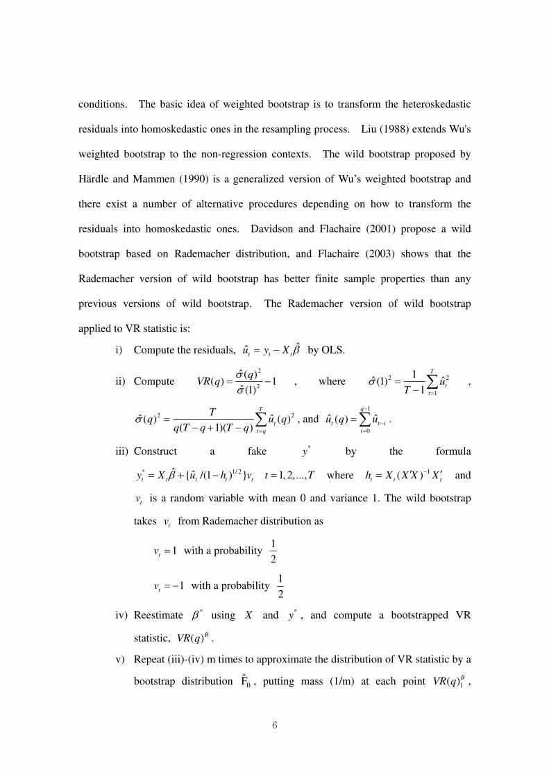
III. Wild-bootstrapped VR Test

A number of bootstrap procedures have been proposed for heteroskedastic

models.4 Wu (1986) proposes so-called ‘weighted bootstrap’ for heteroskedastic data

and shows that the variance estimate by weighted bootstrap is consistent under mild

4 For a review, see Jeong and Maddala (1993).

6

conditions. The basic idea of weighted bootstrap is to transform the heteroskedastic

residuals into homoskedastic ones in the resampling process. Liu (1988) extends Wu's

weighted bootstrap to the non-regression contexts. The wild bootstrap proposed by

Härdle and Mammen (1990) is a generalized version of Wu’s weighted bootstrap and

there exist a number of alternative procedures depending on how to transform the

residuals into homoskedastic ones. Davidson and Flachaire (2001) propose a wild

bootstrap based on Rademacher distribution, and Flachaire (2003) shows that the

Rademacher version of wild bootstrap has better finite sample properties than any

previous versions of wild bootstrap. The Rademacher version of wild bootstrap

applied to VR statistic is:

i) Compute the residuals, ˆˆt t t

u y X β= − by OLS.

ii) Compute 2

2

ˆ ( )( ) 1

ˆ (1)

qVR q

σσ

= − , where 2 2

1

1ˆ ˆ(1)

1

T

t

t

uT

σ=

=− ∑ ,

2 2ˆ ˆ( ) ( )( 1)( )

T

t

t q

Tq u q

q T q T qσ

=

=− + − ∑ , and

1

0

ˆ ˆ( )q

t t i

i

u q u−

−=

=∑ .

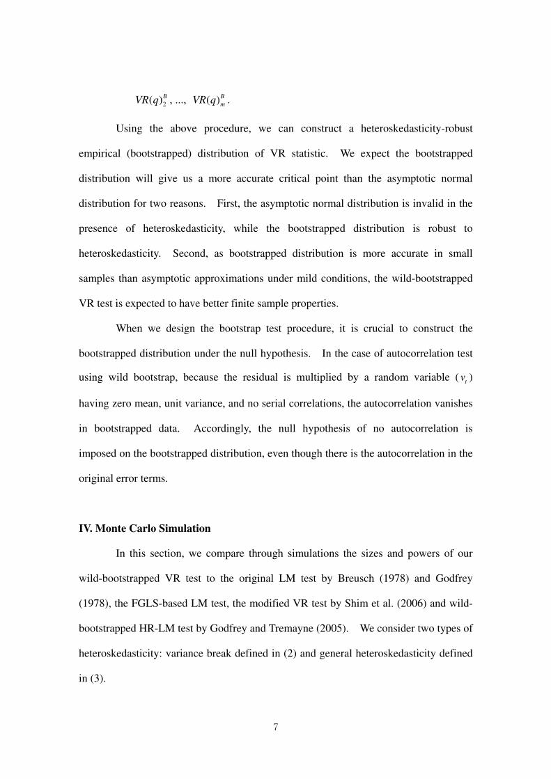
iii) Construct a fake *y by the formula

* 1/ 2ˆ ˆ{ /(1 ) } 1, 2,...,t t t t t

y X u h v t Tβ= + − = where 1( )t t t

h X X X X−′ ′= and

tv is a random variable with mean 0 and variance 1. The wild bootstrap

takes t

v from Rademacher distribution as

1t

v = with a probability 1

2

1t

v = − with a probability 1

2

iv) Reestimate *β using X and *y , and compute a bootstrapped VR

statistic, ( )BVR q .

v) Repeat (iii)-(iv) m times to approximate the distribution of VR statistic by a

bootstrap distribution BF̂ , putting mass (1/m) at each point 1( )BVR q ,

7

2( )BVR q , ..., ( )B

mVR q .

Using the above procedure, we can construct a heteroskedasticity-robust

empirical (bootstrapped) distribution of VR statistic. We expect the bootstrapped

distribution will give us a more accurate critical point than the asymptotic normal

distribution for two reasons. First, the asymptotic normal distribution is invalid in the

presence of heteroskedasticity, while the bootstrapped distribution is robust to

heteroskedasticity. Second, as bootstrapped distribution is more accurate in small

samples than asymptotic approximations under mild conditions, the wild-bootstrapped

VR test is expected to have better finite sample properties.

When we design the bootstrap test procedure, it is crucial to construct the

bootstrapped distribution under the null hypothesis. In the case of autocorrelation test

using wild bootstrap, because the residual is multiplied by a random variable ( tv )

having zero mean, unit variance, and no serial correlations, the autocorrelation vanishes

in bootstrapped data. Accordingly, the null hypothesis of no autocorrelation is

imposed on the bootstrapped distribution, even though there is the autocorrelation in the

original error terms.

IV. Monte Carlo Simulation

In this section, we compare through simulations the sizes and powers of our

wild-bootstrapped VR test to the original LM test by Breusch (1978) and Godfrey

(1978), the FGLS-based LM test, the modified VR test by Shim et al. (2006) and wild-

bootstrapped HR-LM test by Godfrey and Tremayne (2005). We consider two types of

heteroskedasticity: variance break defined in (2) and general heteroskedasticity defined

in (3).

8

1. Variance Break Case

First, let us examine the empirical sizes of the tests. We generate the error

terms t

u ’s to have variance break but no autocorrelation by (2). The fundamental

error terms, t

η ’s are generated from independent N(0,1) and we fix 1 1σ = and handle

the variance shift using 2σ . Two cases can be considered about 2σ : decreasing

variance ( 12 σσ < ) and increasing variance ( 12 σσ > ). For brevity of presentation, we

present the results from decreasing variance case.5 We take (0.25, 0.4, 0.6, 0.8, 1) as

2σ . Various break timings (τ) are considered from 0.05 to 0.95. t

y ’s are generated by

0 1 1 2 2 1,2, ,t t t t

y X X u t Tβ β β= + + + = K (4)

where 0 1 2 1β β β= = = and 1tX , 2t

X follow (0,1)IIN with 1 2cov( , ) 0t t

X X = . We

examine three sample sizes: T=20, T=50, and T=100. Three different lag lengths (p)

of the autoregressive serial correlation are employed: p=1, p=4, and p=8. The nominal

size is set to 5%. The number of simulations is 1000, and the number of bootstrap

resamples is 1,000.

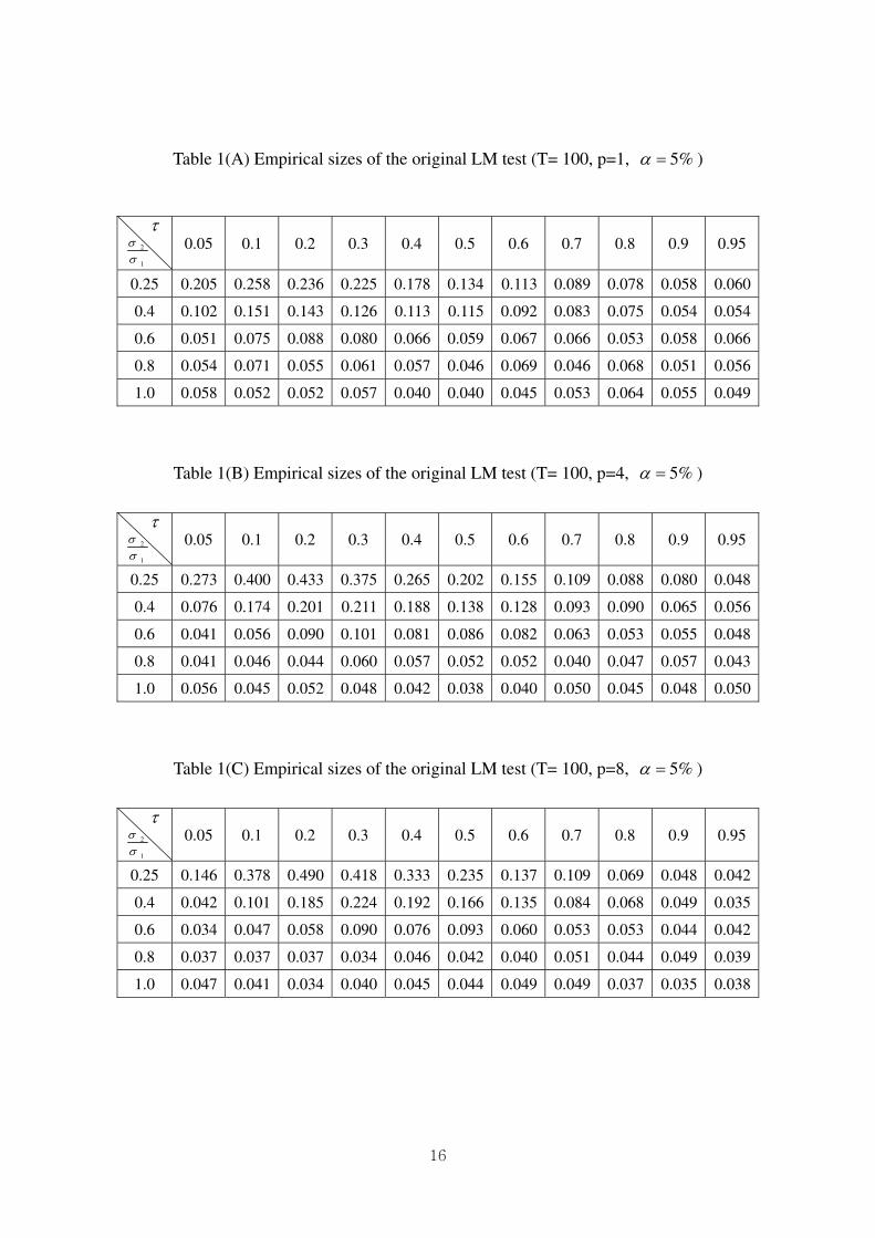
Table 1(A)-(C) confirm the findings of Hyun et al. (2006). Table 1(A) shows

the empirical sizes of B-G LM test in the above setup for p=1, Table 1(B) for p=4, and

Table 1(C) for p=8, respectively. For Tables 1(A)-(C), the sample size is set at T=100.

As shown in the Tables, the empirical sizes of the original LM test are severely distorted

in the presence of variance break. The size distortion becomes more severe as the

variance reduction ratio after the break ( )12 /σσ= intensifies. The size distortion also

depends on the location (τ) of the break as Hyun et al. (2006) show.

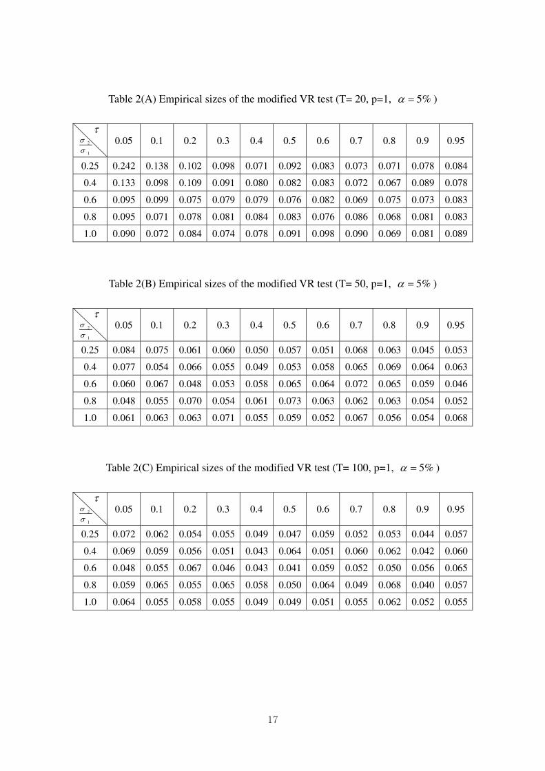
Table 2(A)-(C) show the results of the modified VR test (p=1 and T=20, 50,

100 respectively). When the sample size is as large as 100, Table 2(C) reaffirms the

5 There exist no qualitative differences in increasing variance case. The simulation results are

available from authors upon request.

9

findings of Shim et al. (2006). The empirical sizes are significantly more accurate than

the original LM test in Table 1(C). For example, when τ=0.2 and σ2=0.25, the size of

the modified VR test is 5.4% in Table 2(C) while the size of the original LM test is

23.6% in Table 1(A). When the sample size becomes smaller, however, the empirical

sizes of the modified VR test become inaccurate. When T=50, the empirical sizes in

Table 2(B) show tendency for over-rejection, sometimes as high as 8.4%. When T=20,

the modified VR test seriously over-rejects the null hypothesis as shown in Table 2(A).

In many cases, the empirical sizes are higher than 10%. This is not surprising

considering the VR test uses an asymptotic standard normal distribution, and uses an

asymptotic correction to deal with heteroskedasticity. We will show later that the wild-

bootstrapped tests have significantly better small sample properties than the modified

VR test.

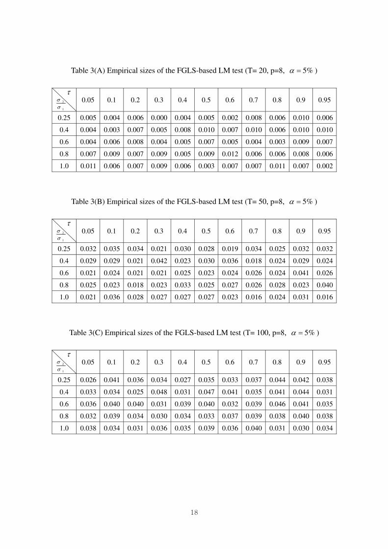
The FGLS-based LM test works better than the modified VR test in this

variance break case. It is natural for FGLS-based LM test to outperform the modified

VR test. The FGLS procedure specifically reflects the variance break pattern in the

first stage, while the modified VR test corrects heteroskedasticity in a general way.

However, the FGLS-based LM test show weak performance when the sample size is

small and the lag length is large. Table 3(A)-(C) show the empirical sizes of FGLS-

based LM test for p=8, and T=20, 50, and 100, respectively. We can see the sizes are

inaccurate especially when T=20 and p=8. We will show later that the two wild-

bootstrapped tests have accurate sizes even when the lag length is as high as p=8.

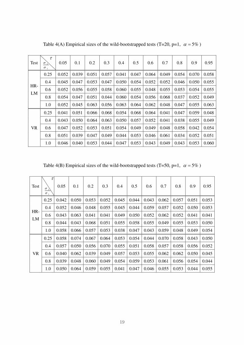
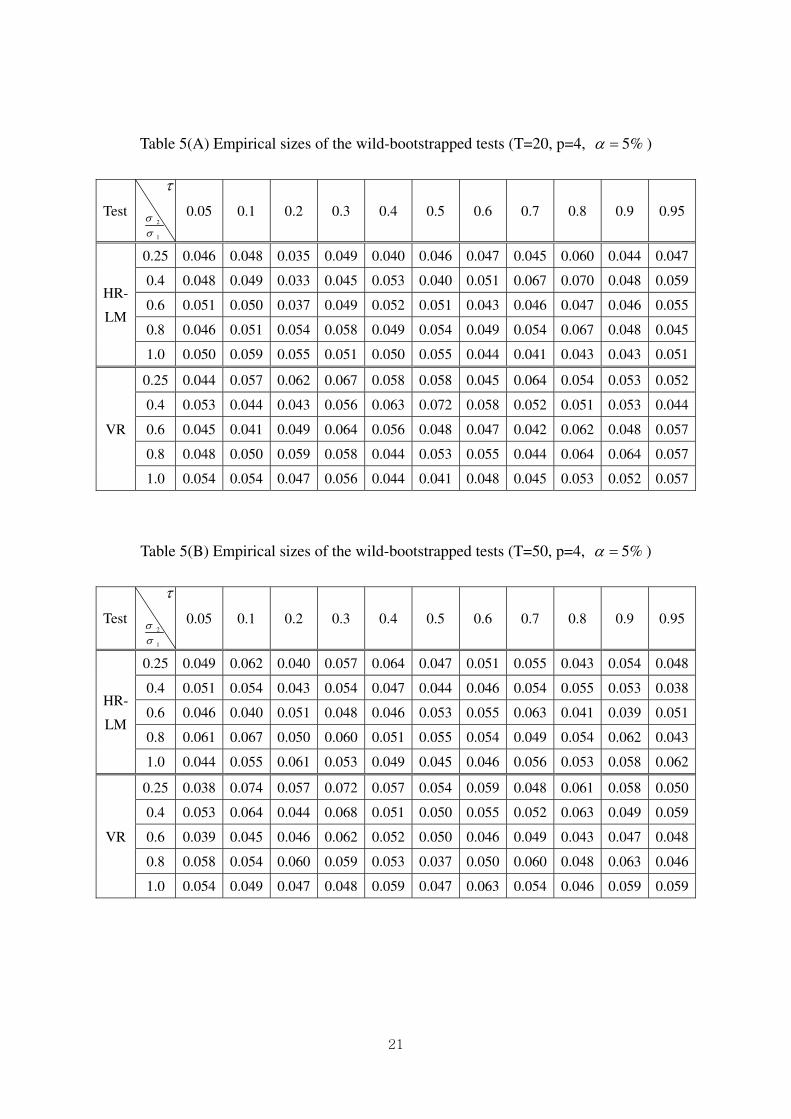
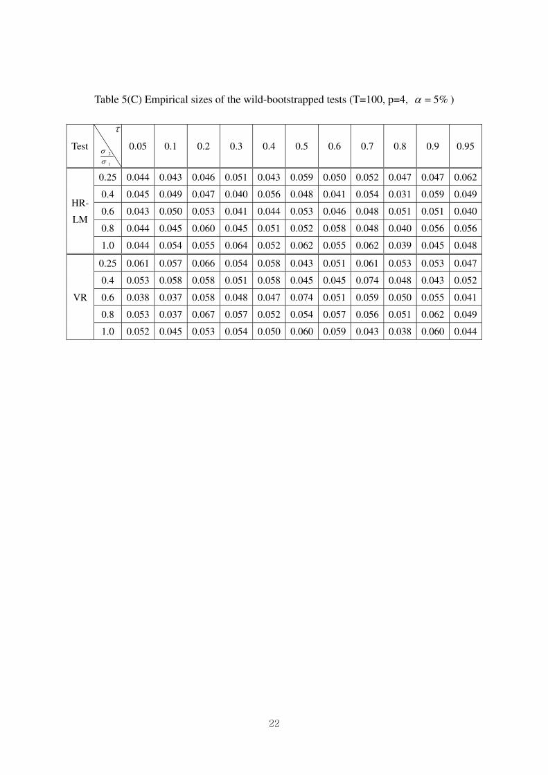
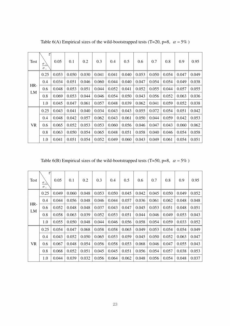
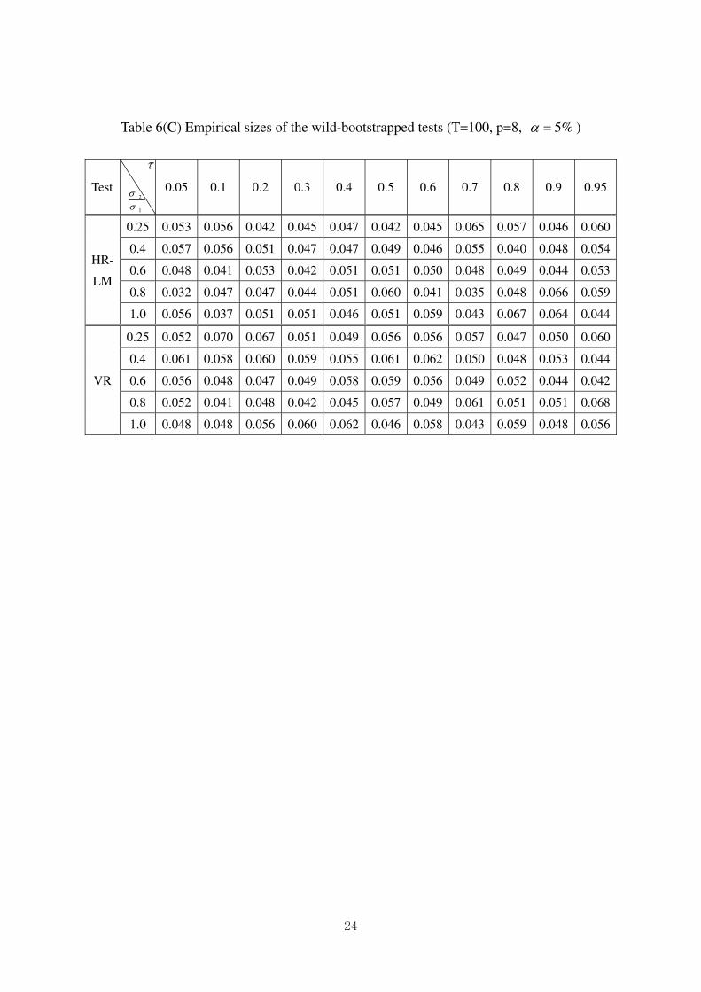
On the other hand, the two wild-bootstrapped tests, our proposed wild-

bootstrapped VR test and the wild-bootstrapped HR-LM test by Godfrey and Tremayne

(2005) have very accurate empirical sizes in the presence of variance break. Tables 4-

10

9 show the empirical sizes of the two tests. Table 4(A)-(C) are for the cases of p=1,

Tables 5(A)-(C) are for p=4, and Tables 6(A)-(C) are for p=8. As shown in the Tables,

the empirical sizes of the wild-bootstrap tests are all close to the nominal size. Even

when the sample size is as small as 20 and the lag length is as high as 8, Table 6(A)

shows that the empirical sizes of the tests are quite accurate. From the Tables 4-6, it is

clear that the wild-bootstrapped tests are robust to the degree of heteroskedasticity

(variance reduction rate), sample size, and the length of lag.

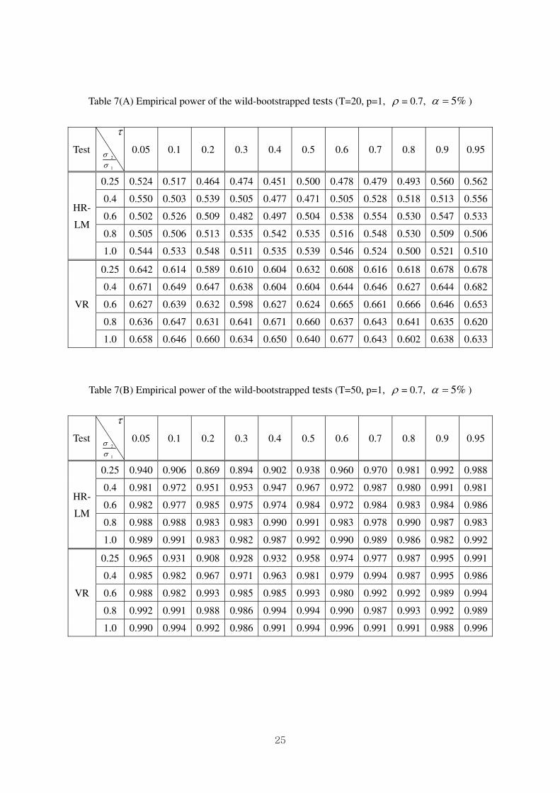
Let us now examine the powers of alternative tests. To consider the power, we

impose autocorrelation as well as heteroskedasticity on error term in the following way:

1t t t tu uρ σ η−= + (5)

2 2 2

1 21[ ] 1[ ]t t T t Tσ σ τ σ τ= ≤ + >

It is noted that the error term now follows AR(1) process and its variance has a

break at Tτ . In the simulation, we use 0.7 for the value of ρ . All the other

parameters are the same as before.

Tables 7-9 present the empirical powers of the two wild-bootstrapped tests.

We only present the results of the wild-bootstrapped tests because the other two tests

fail to control the size in our simulation. Tables 7(A)-(B) are for the cases of lag

length, p=1, Tables 8(A)-(B) are for p=4, and Tables 9(A)-(B) are for the cases of p=8.6

First, we notice from the Tables 7-9 that the empirical powers of the wild-bootstrapped

tests are robust to heteroskedasticity. No matter how high the variance reduction rate

( )12 /σσ= is, the empirical powers are almost the same as the homoskedasticity case of

1/ 12 =σσ . This implies that the wild-bootstrapped tests have resolved the problem of

6 We don’t present the cases of T=100 because the powers of T=100 are very close to 1 in

almost every case. The results are available from the authors upon request.

11

the original LM test: size distortion and power reduction due to heteroskedasticity.

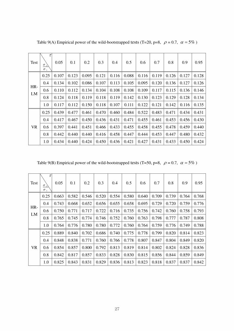
Second, we observe from Table 7-9 that our wild-bootstrapped VR test has

superior small sample properties to the wild-bootstrapped HR-LM test by Godfrey and

Tremayne (2005) in all cases. The wild-bootstrapped VR test show significantly

higher powers and is more robust to the structure of lag length than wild-bootstrapped

HR-LM test. Both the tests show worse power as lag length grows, which is natural

considering we impose AR(1) structure in the simulations. However, even when the

lag length is misspecified, the powers of our wild-bootstrapped VR test are considerably

higher than the wild-bootstrapped HR-LM test. For example, as seen in Tables 9(A),

the powers of the wild-bootstrapped VR (around 0.450 on average) are almost four

times higher than the powers of the wild-bootstrapped HR-LM test (around 0.120 on

average), in the case of p=8 and T=20.

2. General Heteroskedasticity Case

Now, let us consider a more general form of heteroskedasticity than variance

break. All the other parameters of the simulation are the same as variance break case

in the earlier section except for t

u . The error term now is defined by (3), where t

η ’s

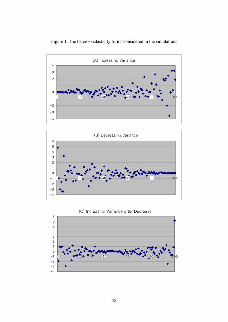
follow (0,1)IIN . To create heteroskedasticity, a random variable tε is drawn from

(0,1)IIN and sorted by three different rules. First, we sort tε ’s by the absolute

values of tε , to create continuously increasing heteroskedasticity. Second, we sort

tε

by the negative of the absolute value, to create continuously decreasing

heteroskedasticity. Last, we sort tε by its raw value, to create heteroskedasticity with

an increase after a decrease. Three forms of heteroskedasticity generated by the rules

are shown in Figure 1(A)-(C).

12

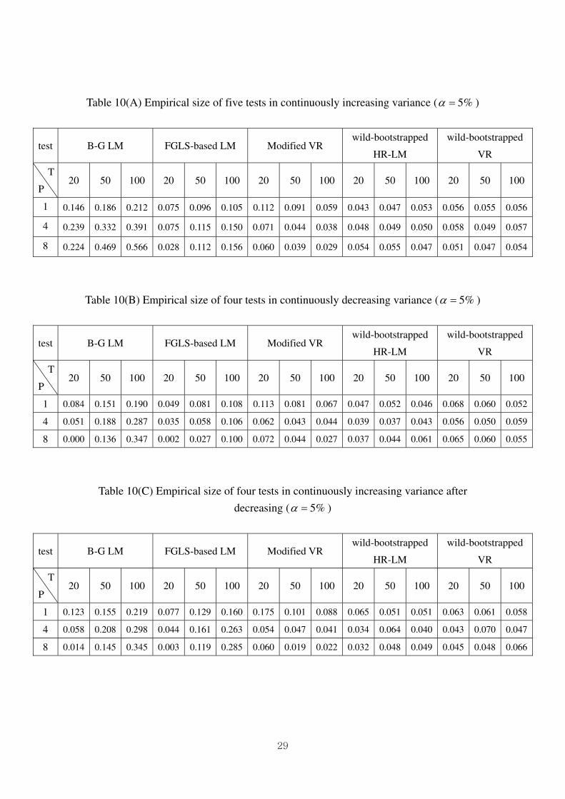
Table 10(A)-(C) show the empirical sizes of the alternative tests in each case of

continuous heteroskedasticity: increasing variances, decreasing variances, and

increasing after decreasing, respectively. As seen in Tables 10(A)-(C), the wild-

bootstrapped VR test and the wild-bootstrapped HR-LM test control the size quite

successfully. The two tests show stable empirical sizes respectively from 0.043 to 0.070

and from 0.032 to 0.065. On the other hand, the original LM test, the FGLS-based LM

test, and the modified VR test all tend to over-reject the true null hypothesis in most

cases and under-reject the null in the cases of small sample and large lag length.7

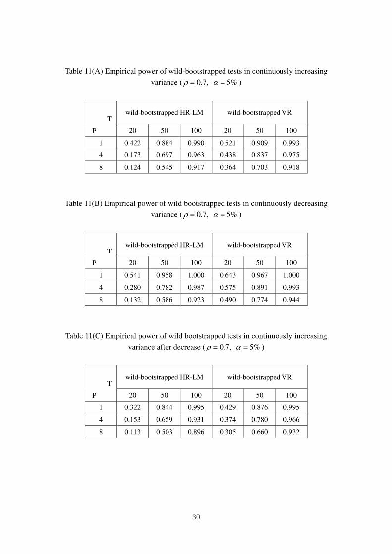
Table 11(A)-(C) show the empirical powers of the two wild-bootstrapped tests.

Considering the sizes of the other tests are considerably distorted, we only present the

empirical powers of the wild-bootstrapped VR test and the wild-bootstrapped HR-LM

test. To compute powers, we impose autocorrelation as well as heteroskedasticity on

the error term in the following way:

tttt uu ηερ += −1 (6)

Note that the error term now follows AR(1) process and its variance has a

continuous heteroskedasticity factor. In the simulation, we set ρ = 0.7. All the other

parameters are the same as before.

We observe from Table 11(A)-(C) that the empirical powers of the two tests in

general heteroskedasticity case show similar patterns to the ones in variance break case.

The wild-bootstrapped VR test always shows significantly higher power and is much

more robust to misspecification of lag length than the wild-bootstrapped HR-LM test by

Godfrey and Tremayne (2005). For example, as seen in Tables 11(B), the power of the

wild-bootstrapped VR is 0.490, almost four times higher than the one of the wild-

7 But the empirical sizes of the modified VR test become much more accurate in larger samples

than T=500. The results are available from the authors upon request.

13

bootstrapped HR-LM test, 0.132, in the case of p=8 and T=20.

VI. Conclusion

We propose a wild-bootstrapped VR test for autocorrelation in the presence of

heteroskedasticity. We also compare the finite sample properties of the test to the

existing tests, such as the original Breusch-Godfrey’s LM test, the FGLS-based LM test

by Shim et al. (2006), the modified VR test by Shim et al. (2006) and the wild-

bootstrapped HR-LM test by Godfrey and Tremayne (2005). The Monte Carlo

simulation shows that the wild-bootstrapped VR test outperforms the existing tests both

in size and power.

14

References

Bai, J., 1993. Least squares estimation of a shift in linear processes, Journal of Time

Series Analysis 15, 453-472

Bai, J., R. Lumsdaine, and J. Stock, 1998. “Testing for and dating common breaks in

multivariate time series,” Review of Economic studies 65, 395-432

Breusch, T., 1978. “Testing for autocorrelation in dynamic linear models,” Australian

Economic Papers 17, 334-335.

Cribari-Neto, F. and S. G. Zarkos, 2003. “Improved weighted bootstrap,” working paper.

Davidson, R. and E. Flachaire, 2001. “The wild bootstrap, tamed at last,” working paper

IER#1000, Queen’s University.

Flachaire, E., 2003. “Bootstrapping heteroskedastic regression models: wild bootstrap

vs. pairs bootstrap,” working paper.

Godfrey, L., 1978. “Testing against general autoregressive and moving average error

models when the regressors include lagged dependent variables,” Econometrica 46,

1293-1302.

Godfrey, L. and A.R. Tremayne, 2005. “The wild bootstrap and heteroskedasticity-

robust tests for serial correlation in dynamic regression models,” Computational

Statistics & Data Analysis 49, 377-395

Härdle, W. and E. Mammen, 1990. “Bootstrap methods in nonparametric regression,”

CORE Discussion Paper No. 9049.

Hyun, J.-H., T.-H. Kim, and J. Jeong, 2006. “The effect of a variance-shift on the

Breusch-Godfrey’s LM test,” working paper, Yonsei University.

Jeong, J., and G.S. Maddala, 1993. “A perspective on application of bootstrap methods

in econometrics,” In: Maddala, G.S., Rao, C.R., Vinod, H.D.(Eds.), Handbook of

Statistics: Econometrics, 11, 573-610.

Liu, R., 1988. “Bootstrap procedures under some non i.i.d. models,” Annals of

Statistics 16, 1696-1708.

15

Lo, A.W., and A.G. MacKinlay, 1988. “Stock market prices do not follow random

walks: evidence from a simple specification test,” Review of Financial Studies 1,

41-66.

Lo, A.W., and A.G. MacKinlay, 1989. “The size and power of the variance ratio test in

finite samples,” Journal of Econometrics 40, 203-238.

Mammen, E., 1993. “Bootstrap and wild bootstrap for high dimensional linear models,”

Annals of Statistics 21, 255-285.

Shim, E.-Y., H.-H. Moon, and T.-H. Kim, 2006. “Autocorrelation tests robust to a

structural break in variance,” working paper, Yonsei University.

Wu, C.F.J., 1986. “Jackknife, bootstrap and other resampling methods in Regression

analysis,” Annals of Statistics 14, 1261-1295.

16

Table 1(A) Empirical sizes of the original LM test (T= 100, p=1, 5%α = )

τ

2

1

σσ

0.05 0.1 0.2 0.3 0.4 0.5 0.6 0.7 0.8 0.9 0.95

0.25 0.205 0.258 0.236 0.225 0.178 0.134 0.113 0.089 0.078 0.058 0.060

0.4 0.102 0.151 0.143 0.126 0.113 0.115 0.092 0.083 0.075 0.054 0.054

0.6 0.051 0.075 0.088 0.080 0.066 0.059 0.067 0.066 0.053 0.058 0.066

0.8 0.054 0.071 0.055 0.061 0.057 0.046 0.069 0.046 0.068 0.051 0.056

1.0 0.058 0.052 0.052 0.057 0.040 0.040 0.045 0.053 0.064 0.055 0.049

Table 1(B) Empirical sizes of the original LM test (T= 100, p=4, 5%α = )

τ

2

1

σσ

0.05 0.1 0.2 0.3 0.4 0.5 0.6 0.7 0.8 0.9 0.95

0.25 0.273 0.400 0.433 0.375 0.265 0.202 0.155 0.109 0.088 0.080 0.048

0.4 0.076 0.174 0.201 0.211 0.188 0.138 0.128 0.093 0.090 0.065 0.056

0.6 0.041 0.056 0.090 0.101 0.081 0.086 0.082 0.063 0.053 0.055 0.048

0.8 0.041 0.046 0.044 0.060 0.057 0.052 0.052 0.040 0.047 0.057 0.043

1.0 0.056 0.045 0.052 0.048 0.042 0.038 0.040 0.050 0.045 0.048 0.050

Table 1(C) Empirical sizes of the original LM test (T= 100, p=8, 5%α = )

τ

2

1

σσ

0.05 0.1 0.2 0.3 0.4 0.5 0.6 0.7 0.8 0.9 0.95

0.25 0.146 0.378 0.490 0.418 0.333 0.235 0.137 0.109 0.069 0.048 0.042

0.4 0.042 0.101 0.185 0.224 0.192 0.166 0.135 0.084 0.068 0.049 0.035

0.6 0.034 0.047 0.058 0.090 0.076 0.093 0.060 0.053 0.053 0.044 0.042

0.8 0.037 0.037 0.037 0.034 0.046 0.042 0.040 0.051 0.044 0.049 0.039

1.0 0.047 0.041 0.034 0.040 0.045 0.044 0.049 0.049 0.037 0.035 0.038

17

Table 2(A) Empirical sizes of the modified VR test (T= 20, p=1, 5%α = )

τ

2

1

σσ

0.05 0.1 0.2 0.3 0.4 0.5 0.6 0.7 0.8 0.9 0.95

0.25 0.242 0.138 0.102 0.098 0.071 0.092 0.083 0.073 0.071 0.078 0.084

0.4 0.133 0.098 0.109 0.091 0.080 0.082 0.083 0.072 0.067 0.089 0.078

0.6 0.095 0.099 0.075 0.079 0.079 0.076 0.082 0.069 0.075 0.073 0.083

0.8 0.095 0.071 0.078 0.081 0.084 0.083 0.076 0.086 0.068 0.081 0.083

1.0 0.090 0.072 0.084 0.074 0.078 0.091 0.098 0.090 0.069 0.081 0.089

Table 2(B) Empirical sizes of the modified VR test (T= 50, p=1, 5%α = )

τ

2

1

σσ

0.05 0.1 0.2 0.3 0.4 0.5 0.6 0.7 0.8 0.9 0.95

0.25 0.084 0.075 0.061 0.060 0.050 0.057 0.051 0.068 0.063 0.045 0.053

0.4 0.077 0.054 0.066 0.055 0.049 0.053 0.058 0.065 0.069 0.064 0.063

0.6 0.060 0.067 0.048 0.053 0.058 0.065 0.064 0.072 0.065 0.059 0.046

0.8 0.048 0.055 0.070 0.054 0.061 0.073 0.063 0.062 0.063 0.054 0.052

1.0 0.061 0.063 0.063 0.071 0.055 0.059 0.052 0.067 0.056 0.054 0.068

Table 2(C) Empirical sizes of the modified VR test (T= 100, p=1, 5%α = )

τ

2

1

σσ

0.05 0.1 0.2 0.3 0.4 0.5 0.6 0.7 0.8 0.9 0.95

0.25 0.072 0.062 0.054 0.055 0.049 0.047 0.059 0.052 0.053 0.044 0.057

0.4 0.069 0.059 0.056 0.051 0.043 0.064 0.051 0.060 0.062 0.042 0.060

0.6 0.048 0.055 0.067 0.046 0.043 0.041 0.059 0.052 0.050 0.056 0.065

0.8 0.059 0.065 0.055 0.065 0.058 0.050 0.064 0.049 0.068 0.040 0.057

1.0 0.064 0.055 0.058 0.055 0.049 0.049 0.051 0.055 0.062 0.052 0.055

18

Table 3(A) Empirical sizes of the FGLS-based LM test (T= 20, p=8, 5%α = )

τ

2

1

σσ

0.05 0.1 0.2 0.3 0.4 0.5 0.6 0.7 0.8 0.9 0.95

0.25 0.005 0.004 0.006 0.000 0.004 0.005 0.002 0.008 0.006 0.010 0.006

0.4 0.004 0.003 0.007 0.005 0.008 0.010 0.007 0.010 0.006 0.010 0.010

0.6 0.004 0.006 0.008 0.004 0.005 0.007 0.005 0.004 0.003 0.009 0.007

0.8 0.007 0.009 0.007 0.009 0.005 0.009 0.012 0.006 0.006 0.008 0.006

1.0 0.011 0.006 0.007 0.009 0.006 0.003 0.007 0.007 0.011 0.007 0.002

Table 3(B) Empirical sizes of the FGLS-based LM test (T= 50, p=8, 5%α = )

τ

2

1

σσ

0.05 0.1 0.2 0.3 0.4 0.5 0.6 0.7 0.8 0.9 0.95

0.25 0.032 0.035 0.034 0.021 0.030 0.028 0.019 0.034 0.025 0.032 0.032

0.4 0.029 0.029 0.021 0.042 0.023 0.030 0.036 0.018 0.024 0.029 0.024

0.6 0.021 0.024 0.021 0.021 0.025 0.023 0.024 0.026 0.024 0.041 0.026

0.8 0.025 0.023 0.018 0.023 0.033 0.025 0.027 0.026 0.028 0.023 0.040

1.0 0.021 0.036 0.028 0.027 0.027 0.027 0.023 0.016 0.024 0.031 0.016

Table 3(C) Empirical sizes of the FGLS-based LM test (T= 100, p=8, 5%α = )

τ

2

1

σσ

0.05 0.1 0.2 0.3 0.4 0.5 0.6 0.7 0.8 0.9 0.95

0.25 0.026 0.041 0.036 0.034 0.027 0.035 0.033 0.037 0.044 0.042 0.038

0.4 0.033 0.034 0.025 0.048 0.031 0.047 0.041 0.035 0.041 0.044 0.031

0.6 0.036 0.040 0.040 0.031 0.039 0.040 0.032 0.039 0.046 0.041 0.035

0.8 0.032 0.039 0.034 0.030 0.034 0.033 0.037 0.039 0.038 0.040 0.038

1.0 0.038 0.034 0.031 0.036 0.035 0.039 0.036 0.040 0.031 0.030 0.034

19

Table 4(A) Empirical sizes of the wild-bootstrapped tests (T=20, p=1, 5%α = )

Test τ

2

1

σσ

0.05 0.1 0.2 0.3 0.4 0.5 0.6 0.7 0.8 0.9 0.95

HR-

LM

0.25 0.052 0.039 0.051 0.057 0.041 0.047 0.064 0.049 0.054 0.070 0.058

0.4 0.045 0.047 0.053 0.047 0.050 0.054 0.052 0.052 0.046 0.050 0.055

0.6 0.052 0.056 0.055 0.058 0.060 0.055 0.048 0.055 0.053 0.054 0.055

0.8 0.054 0.047 0.051 0.044 0.060 0.054 0.056 0.068 0.037 0.052 0.049

1.0 0.052 0.045 0.063 0.056 0.063 0.064 0.062 0.048 0.047 0.055 0.063

VR

0.25 0.041 0.051 0.066 0.068 0.054 0.068 0.064 0.041 0.047 0.059 0.048

0.4 0.043 0.050 0.064 0.063 0.050 0.057 0.052 0.041 0.038 0.055 0.049

0.6 0.047 0.052 0.053 0.051 0.054 0.049 0.049 0.048 0.058 0.042 0.054

0.8 0.051 0.039 0.047 0.049 0.044 0.053 0.046 0.061 0.034 0.052 0.051

1.0 0.046 0.040 0.053 0.044 0.047 0.053 0.043 0.049 0.043 0.053 0.060

Table 4(B) Empirical sizes of the wild-bootstrapped tests (T=50, p=1, 5%α = )

Test

τ 2

1

σσ

0.05 0.1 0.2 0.3 0.4 0.5 0.6 0.7 0.8 0.9 0.95

HR-

LM

0.25 0.042 0.050 0.053 0.052 0.045 0.044 0.043 0.062 0.057 0.051 0.053

0.4 0.052 0.046 0.048 0.055 0.045 0.044 0.059 0.057 0.052 0.050 0.053

0.6 0.043 0.063 0.041 0.041 0.049 0.050 0.052 0.062 0.052 0.041 0.041

0.8 0.044 0.043 0.068 0.051 0.055 0.058 0.055 0.049 0.055 0.053 0.050

1.0 0.058 0.066 0.057 0.053 0.038 0.047 0.043 0.059 0.048 0.049 0.054

VR

0.25 0.058 0.074 0.067 0.064 0.053 0.054 0.044 0.070 0.058 0.043 0.050

0.4 0.057 0.050 0.056 0.070 0.055 0.051 0.058 0.057 0.058 0.056 0.052

0.6 0.040 0.062 0.039 0.049 0.057 0.053 0.055 0.062 0.062 0.050 0.045

0.8 0.039 0.048 0.060 0.049 0.054 0.059 0.053 0.061 0.056 0.054 0.044

1.0 0.050 0.064 0.059 0.055 0.041 0.047 0.046 0.055 0.053 0.044 0.055

20

Table 4(C) Empirical sizes of the wild-bootstrapped tests (T=100, p=1, 5%α = )

Test

τ 2

1

σσ

0.05 0.1 0.2 0.3 0.4 0.5 0.6 0.7 0.8 0.9 0.95

HR-

LM

0.25 0.037 0.052 0.055 0.052 0.050 0.041 0.056 0.052 0.046 0.048 0.053

0.4 0.060 0.057 0.056 0.048 0.047 0.058 0.049 0.062 0.058 0.044 0.049

0.6 0.045 0.054 0.056 0.041 0.039 0.038 0.058 0.057 0.044 0.053 0.060

0.8 0.055 0.066 0.052 0.056 0.051 0.050 0.059 0.041 0.063 0.043 0.055

1.0 0.053 0.050 0.051 0.052 0.041 0.052 0.042 0.056 0.061 0.053 0.050

VR

0.25 0.046 0.054 0.060 0.062 0.053 0.046 0.056 0.049 0.046 0.048 0.053

0.4 0.059 0.062 0.062 0.054 0.044 0.065 0.055 0.063 0.060 0.041 0.056

0.6 0.046 0.054 0.059 0.047 0.041 0.044 0.058 0.054 0.053 0.056 0.058

0.8 0.052 0.064 0.053 0.056 0.053 0.049 0.063 0.046 0.059 0.041 0.050

1.0 0.056 0.051 0.047 0.053 0.042 0.052 0.049 0.051 0.062 0.050 0.048

21


Test

τ 2

1

σσ

0.05 0.1 0.2 0.3 0.4 0.5 0.6 0.7 0.8 0.9 0.95

HR-

LM

0.25 0.046 0.048 0.035 0.049 0.040 0.046 0.047 0.045 0.060 0.044 0.047

0.4 0.048 0.049 0.033 0.045 0.053 0.040 0.051 0.067 0.070 0.048 0.059

0.6 0.051 0.050 0.037 0.049 0.052 0.051 0.043 0.046 0.047 0.046 0.055

0.8 0.046 0.051 0.054 0.058 0.049 0.054 0.049 0.054 0.067 0.048 0.045

1.0 0.050 0.059 0.055 0.051 0.050 0.055 0.044 0.041 0.043 0.043 0.051

VR

0.25 0.044 0.057 0.062 0.067 0.058 0.058 0.045 0.064 0.054 0.053 0.052

0.4 0.053 0.044 0.043 0.056 0.063 0.072 0.058 0.052 0.051 0.053 0.044

0.6 0.045 0.041 0.049 0.064 0.056 0.048 0.047 0.042 0.062 0.048 0.057

0.8 0.048 0.050 0.059 0.058 0.044 0.053 0.055 0.044 0.064 0.064 0.057

1.0 0.054 0.054 0.047 0.056 0.044 0.041 0.048 0.045 0.053 0.052 0.057


Test

τ 2

1

σσ

0.05 0.1 0.2 0.3 0.4 0.5 0.6 0.7 0.8 0.9 0.95

HR-

LM

0.25 0.049 0.062 0.040 0.057 0.064 0.047 0.051 0.055 0.043 0.054 0.048

0.4 0.051 0.054 0.043 0.054 0.047 0.044 0.046 0.054 0.055 0.053 0.038

0.6 0.046 0.040 0.051 0.048 0.046 0.053 0.055 0.063 0.041 0.039 0.051

0.8 0.061 0.067 0.050 0.060 0.051 0.055 0.054 0.049 0.054 0.062 0.043

1.0 0.044 0.055 0.061 0.053 0.049 0.045 0.046 0.056 0.053 0.058 0.062

VR

0.25 0.038 0.074 0.057 0.072 0.057 0.054 0.059 0.048 0.061 0.058 0.050

0.4 0.053 0.064 0.044 0.068 0.051 0.050 0.055 0.052 0.063 0.049 0.059

0.6 0.039 0.045 0.046 0.062 0.052 0.050 0.046 0.049 0.043 0.047 0.048

0.8 0.058 0.054 0.060 0.059 0.053 0.037 0.050 0.060 0.048 0.063 0.046

1.0 0.054 0.049 0.047 0.048 0.059 0.047 0.063 0.054 0.046 0.059 0.059

22


Test

τ 2

1

σσ

0.05 0.1 0.2 0.3 0.4 0.5 0.6 0.7 0.8 0.9 0.95

HR-

LM

0.25 0.044 0.043 0.046 0.051 0.043 0.059 0.050 0.052 0.047 0.047 0.062

0.4 0.045 0.049 0.047 0.040 0.056 0.048 0.041 0.054 0.031 0.059 0.049

0.6 0.043 0.050 0.053 0.041 0.044 0.053 0.046 0.048 0.051 0.051 0.040

0.8 0.044 0.045 0.060 0.045 0.051 0.052 0.058 0.048 0.040 0.056 0.056

1.0 0.044 0.054 0.055 0.064 0.052 0.062 0.055 0.062 0.039 0.045 0.048

VR

0.25 0.061 0.057 0.066 0.054 0.058 0.043 0.051 0.061 0.053 0.053 0.047

0.4 0.053 0.058 0.058 0.051 0.058 0.045 0.045 0.074 0.048 0.043 0.052

0.6 0.038 0.037 0.058 0.048 0.047 0.074 0.051 0.059 0.050 0.055 0.041

0.8 0.053 0.037 0.067 0.057 0.052 0.054 0.057 0.056 0.051 0.062 0.049

1.0 0.052 0.045 0.053 0.054 0.050 0.060 0.059 0.043 0.038 0.060 0.044

23


Test

τ 2

1

σσ

0.05 0.1 0.2 0.3 0.4 0.5 0.6 0.7 0.8 0.9 0.95

HR-

LM

0.25 0.053 0.050 0.030 0.041 0.041 0.040 0.053 0.050 0.054 0.047 0.049

0.4 0.034 0.051 0.046 0.060 0.044 0.040 0.047 0.054 0.054 0.049 0.038

0.6 0.048 0.053 0.051 0.044 0.052 0.041 0.052 0.055 0.044 0.057 0.055

0.8 0.069 0.053 0.044 0.046 0.054 0.050 0.043 0.056 0.052 0.063 0.036

1.0 0.045 0.047 0.061 0.057 0.048 0.039 0.062 0.041 0.059 0.052 0.038

VR

0.25 0.043 0.041 0.040 0.034 0.043 0.043 0.055 0.072 0.054 0.051 0.042

0.4 0.048 0.042 0.057 0.062 0.043 0.061 0.050 0.044 0.059 0.042 0.053

0.6 0.065 0.052 0.053 0.053 0.060 0.056 0.046 0.047 0.043 0.060 0.062

0.8 0.063 0.050 0.054 0.065 0.048 0.051 0.058 0.040 0.046 0.054 0.058

1.0 0.041 0.051 0.054 0.052 0.049 0.060 0.043 0.049 0.061 0.054 0.051


Test

τ 2

1

σσ

0.05 0.1 0.2 0.3 0.4 0.5 0.6 0.7 0.8 0.9 0.95

HR-

LM

0.25 0.049 0.060 0.048 0.053 0.050 0.045 0.042 0.045 0.050 0.049 0.052

0.4 0.044 0.056 0.048 0.046 0.044 0.057 0.036 0.061 0.062 0.048 0.048

0.6 0.052 0.048 0.048 0.037 0.043 0.047 0.045 0.053 0.051 0.048 0.051

0.8 0.058 0.063 0.039 0.052 0.053 0.051 0.044 0.046 0.049 0.053 0.043

1.0 0.055 0.050 0.048 0.044 0.046 0.056 0.058 0.054 0.059 0.033 0.052

VR

0.25 0.054 0.047 0.068 0.058 0.058 0.065 0.049 0.053 0.054 0.054 0.049

0.4 0.043 0.052 0.050 0.065 0.053 0.059 0.045 0.050 0.052 0.063 0.047

0.6 0.067 0.048 0.054 0.056 0.058 0.053 0.068 0.046 0.047 0.055 0.043

0.8 0.068 0.052 0.051 0.045 0.045 0.051 0.056 0.054 0.057 0.038 0.053

1.0 0.044 0.039 0.032 0.056 0.064 0.062 0.048 0.056 0.054 0.048 0.037

24


Test

τ 2

1

σσ

0.05 0.1 0.2 0.3 0.4 0.5 0.6 0.7 0.8 0.9 0.95

HR-

LM

0.25 0.053 0.056 0.042 0.045 0.047 0.042 0.045 0.065 0.057 0.046 0.060

0.4 0.057 0.056 0.051 0.047 0.047 0.049 0.046 0.055 0.040 0.048 0.054

0.6 0.048 0.041 0.053 0.042 0.051 0.051 0.050 0.048 0.049 0.044 0.053

0.8 0.032 0.047 0.047 0.044 0.051 0.060 0.041 0.035 0.048 0.066 0.059

1.0 0.056 0.037 0.051 0.051 0.046 0.051 0.059 0.043 0.067 0.064 0.044

VR

0.25 0.052 0.070 0.067 0.051 0.049 0.056 0.056 0.057 0.047 0.050 0.060

0.4 0.061 0.058 0.060 0.059 0.055 0.061 0.062 0.050 0.048 0.053 0.044

0.6 0.056 0.048 0.047 0.049 0.058 0.059 0.056 0.049 0.052 0.044 0.042

0.8 0.052 0.041 0.048 0.042 0.045 0.057 0.049 0.061 0.051 0.051 0.068

1.0 0.048 0.048 0.056 0.060 0.062 0.046 0.058 0.043 0.059 0.048 0.056

25

Table 7(A) Empirical power of the wild-bootstrapped tests (T=20, p=1, ρ = 0.7, 5%α = )

Test

τ 2

1

σσ

0.05 0.1 0.2 0.3 0.4 0.5 0.6 0.7 0.8 0.9 0.95

HR-

LM

0.25 0.524 0.517 0.464 0.474 0.451 0.500 0.478 0.479 0.493 0.560 0.562

0.4 0.550 0.503 0.539 0.505 0.477 0.471 0.505 0.528 0.518 0.513 0.556

0.6 0.502 0.526 0.509 0.482 0.497 0.504 0.538 0.554 0.530 0.547 0.533

0.8 0.505 0.506 0.513 0.535 0.542 0.535 0.516 0.548 0.530 0.509 0.506

1.0 0.544 0.533 0.548 0.511 0.535 0.539 0.546 0.524 0.500 0.521 0.510

VR

0.25 0.642 0.614 0.589 0.610 0.604 0.632 0.608 0.616 0.618 0.678 0.678

0.4 0.671 0.649 0.647 0.638 0.604 0.604 0.644 0.646 0.627 0.644 0.682

0.6 0.627 0.639 0.632 0.598 0.627 0.624 0.665 0.661 0.666 0.646 0.653

0.8 0.636 0.647 0.631 0.641 0.671 0.660 0.637 0.643 0.641 0.635 0.620

1.0 0.658 0.646 0.660 0.634 0.650 0.640 0.677 0.643 0.602 0.638 0.633

Table 7(B) Empirical power of the wild-bootstrapped tests (T=50, p=1, ρ = 0.7, 5%α = )

Test

τ 2

1

σσ

0.05 0.1 0.2 0.3 0.4 0.5 0.6 0.7 0.8 0.9 0.95

HR-

LM

0.25 0.940 0.906 0.869 0.894 0.902 0.938 0.960 0.970 0.981 0.992 0.988

0.4 0.981 0.972 0.951 0.953 0.947 0.967 0.972 0.987 0.980 0.991 0.981

0.6 0.982 0.977 0.985 0.975 0.974 0.984 0.972 0.984 0.983 0.984 0.986

0.8 0.988 0.988 0.983 0.983 0.990 0.991 0.983 0.978 0.990 0.987 0.983

1.0 0.989 0.991 0.983 0.982 0.987 0.992 0.990 0.989 0.986 0.982 0.992

VR

0.25 0.965 0.931 0.908 0.928 0.932 0.958 0.974 0.977 0.987 0.995 0.991

0.4 0.985 0.982 0.967 0.971 0.963 0.981 0.979 0.994 0.987 0.995 0.986

0.6 0.988 0.982 0.993 0.985 0.985 0.993 0.980 0.992 0.992 0.989 0.994

0.8 0.992 0.991 0.988 0.986 0.994 0.994 0.990 0.987 0.993 0.992 0.989

1.0 0.990 0.994 0.992 0.986 0.991 0.994 0.996 0.991 0.991 0.988 0.996

26


Test

τ 2

1

σσ

0.05 0.1 0.2 0.3 0.4 0.5 0.6 0.7 0.8 0.9 0.95

HR-

LM

0.25 0.241 0.195 0.213 0.201 0.205 0.210 0.214 0.238 0.222 0.237 0.243

0.4 0.218 0.222 0.207 0.208 0.209 0.217 0.218 0.240 0.234 0.263 0.235

0.6 0.207 0.228 0.206 0.206 0.202 0.229 0.226 0.251 0.254 0.221 0.238

0.8 0.216 0.214 0.222 0.212 0.219 0.234 0.216 0.229 0.224 0.222 0.211

1.0 0.239 0.217 0.238 0.224 0.214 0.200 0.206 0.232 0.237 0.213 0.227

VR

0.25 0.498 0.595 0.561 0.480 0.571 0.542 0.534 0.562 0.560 0.538 0.519

0.4 0.484 0.561 0.539 0.502 0.541 0.523 0.540 0.559 0.559 0.530 0.529

0.6 0.540 0.541 0.526 0.489 0.522 0.550 0.533 0.548 0.556 0.513 0.545

0.8 0.540 0.520 0.521 0.515 0.502 0.524 0.514 0.539 0.526 0.534 0.514

1.0 0.515 0.499 0.543 0.493 0.529 0.529 0.512 0.520 0.542 0.519 0.538


Test

τ 2

1

σσ

0.05 0.1 0.2 0.3 0.4 0.5 0.6 0.7 0.8 0.9 0.95

HR-

LM

0.25 0.843 0.798 0.706 0.707 0.725 0.764 0.823 0.857 0.899 0.921 0.914

0.4 0.889 0.858 0.818 0.801 0.817 0.830 0.862 0.885 0.901 0.908 0.931

0.6 0.902 0.926 0.872 0.898 0.891 0.902 0.896 0.904 0.909 0.920 0.931

0.8 0.911 0.894 0.913 0.908 0.911 0.902 0.903 0.911 0.903 0.914 0.921

1.0 0.913 0.904 0.920 0.917 0.900 0.906 0.918 0.897 0.921 0.912 0.932

VR

0.25 0.956 0.884 0.828 0.844 0.864 0.902 0.912 0.933 0.957 0.957 0.952

0.4 0.962 0.942 0.901 0.900 0.916 0.914 0.930 0.945 0.952 0.955 0.953

0.6 0.957 0.961 0.940 0.954 0.950 0.936 0.949 0.949 0.955 0.950 0.957

0.8 0.965 0.948 0.953 0.948 0.959 0.949 0.947 0.947 0.961 0.959 0.952

1.0 0.942 0.951 0.947 0.960 0.945 0.948 0.954 0.947 0.963 0.949 0.959

27


Test

τ 2

1

σσ

0.05 0.1 0.2 0.3 0.4 0.5 0.6 0.7 0.8 0.9 0.95

HR-

LM

0.25 0.107 0.123 0.095 0.121 0.116 0.088 0.116 0.119 0.126 0.127 0.128

0.4 0.134 0.102 0.086 0.107 0.113 0.105 0.095 0.120 0.136 0.127 0.126

0.6 0.110 0.112 0.134 0.104 0.108 0.108 0.109 0.117 0.115 0.136 0.146

0.8 0.124 0.118 0.119 0.118 0.119 0.142 0.130 0.123 0.129 0.128 0.134

1.0 0.117 0.112 0.150 0.118 0.107 0.111 0.122 0.121 0.142 0.116 0.135

VR

0.25 0.439 0.477 0.461 0.470 0.460 0.484 0.522 0.483 0.471 0.434 0.431

0.4 0.417 0.467 0.450 0.436 0.431 0.471 0.455 0.461 0.453 0.456 0.430

0.6 0.397 0.441 0.451 0.466 0.433 0.455 0.458 0.455 0.478 0.459 0.440

0.8 0.442 0.440 0.440 0.416 0.458 0.447 0.444 0.453 0.447 0.480 0.432

1.0 0.434 0.440 0.424 0.450 0.436 0.421 0.427 0.431 0.433 0.450 0.424


Test

τ 2

1

σσ

0.05 0.1 0.2 0.3 0.4 0.5 0.6 0.7 0.8 0.9 0.95

HR-

LM

0.25 0.663 0.582 0.546 0.520 0.554 0.580 0.640 0.709 0.739 0.764 0.768

0.4 0.743 0.668 0.652 0.656 0.655 0.658 0.695 0.729 0.720 0.759 0.776

0.6 0.750 0.771 0.717 0.722 0.716 0.735 0.756 0.742 0.760 0.758 0.793

0.8 0.765 0.745 0.774 0.746 0.752 0.760 0.763 0.798 0.777 0.787 0.808

1.0 0.764 0.776 0.780 0.780 0.772 0.760 0.764 0.759 0.776 0.749 0.788

VR

0.25 0.889 0.840 0.702 0.686 0.740 0.775 0.778 0.799 0.820 0.814 0.823

0.4 0.848 0.838 0.771 0.760 0.766 0.778 0.807 0.847 0.804 0.849 0.820

0.6 0.854 0.857 0.800 0.792 0.813 0.819 0.814 0.802 0.824 0.828 0.836

0.8 0.842 0.817 0.857 0.833 0.828 0.830 0.815 0.856 0.844 0.859 0.849

1.0 0.825 0.843 0.831 0.829 0.836 0.813 0.823 0.818 0.837 0.837 0.842

28

Figure 1. The heteroskedasticity forms considered in the simulations

-4

-3

-2

-1

0

1

2

3

4

0 20 40 60 80 100

(A) Increasing Variance

-4

-3

-2

-1

0

1

2

3

4

5

6

0 20 40 60 80 100

(B) Decreasing Variance

-4

-3

-2

-1

0

1

2

3

4

5

6

7

0 20 40 60 80 100

(C) Increasing Variance after Decrease

29

Table 10(A) Empirical size of five tests in continuously increasing variance ( 5%α = )

test B-G LM FGLS-based LM Modified VR wild-bootstrapped

HR-LM

wild-bootstrapped

VR

T

P 20 50 100 20 50 100 20 50 100 20 50 100 20 50 100

1 0.146 0.186 0.212 0.075 0.096 0.105 0.112 0.091 0.059 0.043 0.047 0.053 0.056 0.055 0.056

4 0.239 0.332 0.391 0.075 0.115 0.150 0.071 0.044 0.038 0.048 0.049 0.050 0.058 0.049 0.057

8 0.224 0.469 0.566 0.028 0.112 0.156 0.060 0.039 0.029 0.054 0.055 0.047 0.051 0.047 0.054

Table 10(B) Empirical size of four tests in continuously decreasing variance ( 5%α = )


HR-LM

wild-bootstrapped

VR

T

P 20 50 100 20 50 100 20 50 100 20 50 100 20 50 100

1 0.084 0.151 0.190 0.049 0.081 0.108 0.113 0.081 0.067 0.047 0.052 0.046 0.068 0.060 0.052

4 0.051 0.188 0.287 0.035 0.058 0.106 0.062 0.043 0.044 0.039 0.037 0.043 0.056 0.050 0.059

8 0.000 0.136 0.347 0.002 0.027 0.100 0.072 0.044 0.027 0.037 0.044 0.061 0.065 0.060 0.055

Table 10(C) Empirical size of four tests in continuously increasing variance after

decreasing ( 5%α = )


HR-LM

wild-bootstrapped

VR

T

P 20 50 100 20 50 100 20 50 100 20 50 100 20 50 100

1 0.123 0.155 0.219 0.077 0.129 0.160 0.175 0.101 0.088 0.065 0.051 0.051 0.063 0.061 0.058

4 0.058 0.208 0.298 0.044 0.161 0.263 0.054 0.047 0.041 0.034 0.064 0.040 0.043 0.070 0.047

8 0.014 0.145 0.345 0.003 0.119 0.285 0.060 0.019 0.022 0.032 0.048 0.049 0.045 0.048 0.066

30

Table 11(A) Empirical power of wild-bootstrapped tests in continuously increasing

variance ( ρ = 0.7, 5%α = )

T

P

wild-bootstrapped HR-LM wild-bootstrapped VR

20 50 100 20 50 100

1 0.422 0.884 0.990 0.521 0.909 0.993

4 0.173 0.697 0.963 0.438 0.837 0.975

8 0.124 0.545 0.917 0.364 0.703 0.918

Table 11(B) Empirical power of wild bootstrapped tests in continuously decreasing

variance ( ρ = 0.7, 5%α = )

T

P


20 50 100 20 50 100

1 0.541 0.958 1.000 0.643 0.967 1.000

4 0.280 0.782 0.987 0.575 0.891 0.993

8 0.132 0.586 0.923 0.490 0.774 0.944

Table 11(C) Empirical power of wild bootstrapped tests in continuously increasing

variance after decrease ( ρ = 0.7, 5%α = )

T

P


20 50 100 20 50 100

1 0.322 0.844 0.995 0.429 0.876 0.995

4 0.153 0.659 0.931 0.374 0.780 0.966

8 0.113 0.503 0.896 0.305 0.660 0.932

Documents

Wild-Bootstrapped Variance Ratio Test for Autocorrelation in the