1

Wind Sea and Swell Waves in the Nordic Seas

Alvaro Semedo1,2 Escola Naval-CINAV, Lisbon, Portugal.

Roberto Vettor

Centre for Marine Technology and Engineering (CENTEC), Instituto Superior Técnico, University of Lisbon, Lisbon, Portugal.

Øyvind Breivik

European Centre for Medium-Range Weather Forecasts, Reading, United Kingdom

Andreas Sterl Royal Netherlands Meteorological Institute (KNMI), De Bilt, Netherlands

Magnar Reistad

Norwegian Meteorological Institute, Oslo, Norway

Carlos Guedes Soares Centre for Marine Technology and Engineering (CENTEC),

Instituto Superior Técnico, University of Lisbon, Lisbon, Portugal. 1. Introduction

The waves at the ocean surface are the most obvious air-sea interaction phenomena at the interface between the atmosphere and the ocean. These wind waves (henceforth simple called waves) account for most of the energy carried by all waves at the ocean surface (Kinsman 1965), and have a significant impact on coastal infrastructures, ship design and routing, coastal erosion and sediment transport, and are an important element in storm surges and flooding events. Two types of ocean waves can be identified at the ocean surface: wind sea and swell. Wind sea waves are waves under the influence of local winds. As waves propagate from their generation area, or when their phase speed is higher than the local wind speed, they are called swell. Swell waves can propagate thousands of kilometers across entire ocean basins (Snodgrass et al. 1966; Alves 2006).

The significant wave height (SWH) and the mean wave period (MWP) are the most common parameters used to characterize sea states. But these parameters provide a limited description of the wave field, since they are calculated by integrating the wave

1 Corresponding author address: Alvaro Semedo, Escola Naval-CINAV, Base Naval de Lisboa, Alfeite, 2810-001 Almada, Portugal. E-mail: milho.semedo@marinha.pt 2 Also affiliated with: Centre for Marine Technology and Engineering (CENTEC), Instituto Superior Técnico, University of Lisbon, Lisbon, Portugal, and to Department of Earth Sciences, Uppsala University, Sweden.

2

spectra, and two wave fields with the same SWH and MWP may still be different in detail. A mixed sea state of wind sea and swell waves can have the same SWH and MWP as a more young sea state with a strong prevalence of wind seas almost without swell (Holthuijsen 2007, Semedo et al. 2011). For this reason a more detailed investigation and qualitative analysis of the wave field is needed to correctly define the wave characteristics of a certain area. The way to pursuit this analysis is by studying the wind sea and swell parameters separately [SWH and MWP, but also mean wave direction (MWD)].

Several recent studies have looked at the qualitative separation of ocean surface waves has been the focus of several recent climatological studies (Chen et al. 2002, Gulev and Gregorieva 2006, Semedo et al. 2011, Jiang and Chen 2013). Some other studies, following an air sea interaction perspective (Smedman et al. 2009, Högström et al. 2009, Semedo et al. 2009) have also looked at the wind sea and swell separation of the ocean surface. The reason for this interest from the air-sea interaction community lies mostly on the fact that waves have an impact on the lower atmosphere, and that the air-sea coupling is different depending on the wave regime. Waves modulate the exchange of momentum, heat, and mass across the air-sea interface and this modulation is different, depending on the prevalence of one type of waves: wind sea or swell (Högstrom et al. 2009, Semedo et al. 2009).

The goal of the present study is to present a climatology of wind sea and swell characteristics in the Nordic Seas (North Sea, Norwegian Sea, and Barents Sea), based on the high resolution Norwegian Reanalysis at 10 km (NORA10; Reistad et al. 2011), following a similar methodology as Semedo et al (2011). The NORA 10 is a dynamically downscaled version of the ERA-40 reanalysis (Uppala et al. 2005), which comprises atmospheric and wave parameters. The regional distribution of the wind sea and swell SWH and MWD parameters from NORA10, and how they combine in the total SWH and MWP, are presented. 2. Data and analysis methodology a. NORA10

The NORA 10 is a 3-hourly atmospheric and wave high resolution regional reanalysis, produced with the dynamic downscaling of the European Centre for Medium-Range Weather Forecasts (ECMWF) ERA-40 reanalysis. The ERA-40 covers a period from September 1957 to August 2002. Although the NORA 10 is continuously being extended after 2002 using operation analyses from the ECMWF as boundary and initial conditions, here we use only the NORA10 period coincident with ERA-40 (1958-2001), for homogeneity purposes but also to allow some degree of comparison with the results in Semedo et al. (2011).

The NORA10 atmospheric reanalysis was produced with the hydrostatic High-Resolution Limited Area Model (HIRLAM; Undén et al. 2002) at 10-11 km resolution (HIRLAM10), with 40 vertical levels, denser at the surface. The NORA10 model domain was set up as a rotated spherical grid, with a false South Pole (Reistad et al. 2011, their Figure 1).

The wave component of the NORA10 was produced by forcing the wave model WAM (cycle 4; WAMDI Group 1988; Komen et al. 1994) with HIRLAM10 winds on the same domain as the atmospheric model domain. An inner wave model domain was nested into a larger 50 km resolution domain that generated swell boundary conditions. The outer domain was forced with ERA-40 winds. Ice coverage information was passed

3

to the wave model from HIRLAM10 three times per month. Both outer and inner domains were integrated with the bottom friction mode on. Further details and results on NORA 10 can be seen in Reistad et al. (2011) and Aarnes (2011). b. Wave parameters and spectral separation

The wave model WAM outputs two-dimensional wave energy spectra 𝐹(𝑓,𝜃) at each grid point by integrating the so called wave energy balance equation, where 𝑓 and 𝜃 are the wave frequency and propagating direction, respectively. From the wave energy spectra several integrated wave parameters can be obtained. Here SWH, and MWD (mean wave direction) from the total (𝐻𝑠, 𝜃𝑚), wind sea (𝐻𝑠𝑤,𝜃𝑚𝑤) and swell (𝐻𝑠𝑠, 𝜃𝑚𝑠 ) wave fields, respectively, are used. Besides the wave fields the NORA10 10 m wind speed (𝑈10) and direction (𝜑) are also used. The SWH (Munk 1944) is defined as 𝑆𝑊𝐻 = 𝐻𝑠 = 4.04�𝑚0, where 𝑚0 is the zeroth spectral moment defined as 𝑚0 = ∬𝑓0 𝐹(𝑓,𝜃)𝑑𝑓𝑑𝜃, (1) and the MWD is defined as 𝜃𝑚 = atan (𝑆𝐹 𝐶𝐹)⁄ , where 𝑆𝐹 = ∬ sin (𝜃)𝐹(𝑓,𝜃)𝑑𝑓𝑑𝜃 and (2a) 𝐶𝐹 = ∬ cos (𝜃)𝐹(𝑓,𝜃)𝑑𝑓𝑑𝜃. (2b)

In the wave model WAM the wind sea and swell parameters are obtained by integrating the high and low frequency parts of the wave spectra, respectively. The spectral partitioning is obtained through a separation frequency 𝑓, with a correspondent wave phase speed defined as �̂� = 33.6 × 𝑢∗cos (𝜃 − 𝜑) (3) where 𝑢∗ is the friction velocity. See Bidlot (2001) and Semedo et al (2011) for further details on the wind sea and swell separation scheme. 3. The Nordic Seas wind sea and swell climates

The wind and wave parameters were processed for seasonal means: December-January-February (DJF), March-April-May (MAM), June-July-August (JJA), and September-October-November (SON). In spite of some mentions in the text to the intermediate seasons MAM and SON, we will only look at the DJF and JJA seasons (Boreal winter and summer, respectively).

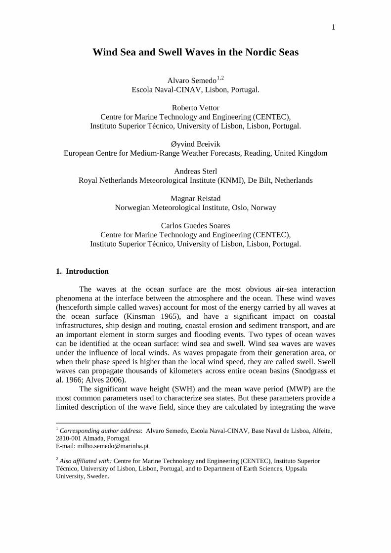
Figure 1 shows the seasonal maps of the DJF and JJA 𝑈10 and 𝜑 (arrows) climatological means are shown. During the winter the mean 10 m-wind speed is higher than 11 m.s-1 in almost all the Nordic Seas, including in the North Sea, and higher than 12 m.s-1 in an area south of Iceland. In the summer the climatological mean 𝑈10 is lower (less than 7 m.s-1 in most of the area), with a maximum (around 9 m.s-1) also south of Iceland. The Norwegian Sea is the preferred track of the extratropical storms in the North Atlantic (Chang et al. 2002; Bengtsson et al. 2006), as can be seen in the southern areas of the domain. South of Iceland the 10 m-winds blow from southwest, as part of

4

the North Atlantic Westerlies, slightly turning counter-clockwise as they enter the Norwegian Sea, both in DJF and JJA. The convergence of the Westerlies with the Polar Easterlies can be seen in both seasons, taking place slightly farther North in JJA. Mesoscale features can be seen in the Barents Sea in both seasons, and along the

a)

b)

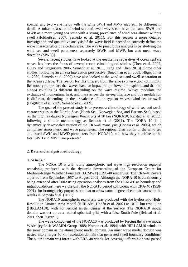
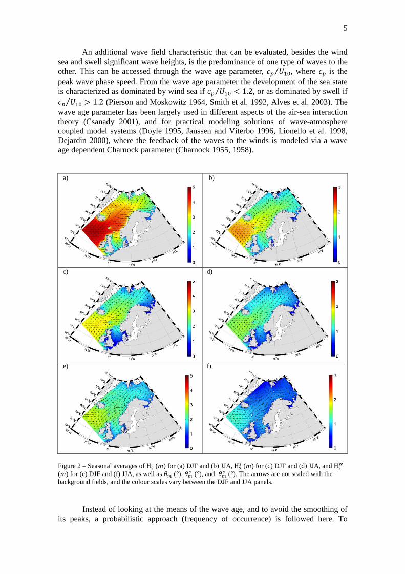
Figure 1 – Seasonal averages of U10 (𝑚 𝑠−1) and 𝜑 (°) for (a) DJF and (b) JJA. The arrows are not scaled with the background fields. western coast of Norway in JJA (most probably sea breezes). A slight increase in the 𝑈10 in the Nordic Seas in DJF and JJA is noticeable when compared to ERA-40 (see Semedo et al 2011), as expected from the validation of the NORA10 shown in Reistad et al. (2011). The seasonal maps of the 𝐻𝑠,𝐻𝑠𝑠, and 𝐻𝑠𝑤 (as well as of 𝜃𝑚,𝜃𝑚𝑤, and 𝜃𝑚𝑠 , represented as arrows) climatological means for DJF and JJA can be seen in Figure 2. While in the open ocean 𝐻𝑠𝑠 is considerably higher than 𝐻𝑠𝑤, as shown by Semedo et al. (2011) and Jiang and Chen (2013), that is not necessarily the case in smaller and constrained areas like marginal seas, where the fetches are limited and swell waves might not have space to propagate away from their generation area. In the Boreal winter the mean 𝐻𝑠𝑠 and 𝐻𝑠𝑤 are relatively comparable, with swell waves propagating into the Norwegian Sea, away from the 𝐻𝑠 climatological maximum south of Iceland. In both seasons, south of Iceland, 𝐻𝑠𝑠 is slightly higher than 𝐻𝑠𝑤 (about 3 m and 2.5 m, in DJF, and 1.5 m and 1 m, in JJA, respectively). That does not happen in the North Sea, where swells are higher than wind sea waves in the winter (1 m and less, and around 2m, respectively), and have about the same mean height in the summer (close to 1 m). In that marginal sea, due to its shape and to the sheltering effect of Great Britain, the 𝐻𝑠𝑠 mean, in DJF to JJA is almost the same, regardless of the differences in the open ocean and in the Norwegian Sea, and swell waves are actually slightly higher in the summer. In the northern part of the Norwegian Sea and in the Barents Sea the mean 𝐻𝑠𝑠 is also practically the same in both seasons. That is not the case for the mean 𝐻𝑠𝑤. Swells are slightly higher than wind seas in DJF in the north part of the Norwegian Sea (around 2.5 and 2.1, respectively), but lower in most parts of the Barents Sea in the same season, also due to a sheltering effect. In JJA the 𝐻𝑠𝑠 mean is higher than 𝐻𝑠𝑤 in that area. As can be seen the sheltering effect and the orientation of the fetch, compared to the coast lines and to the mean wind direction, are very important in defining the swell and wind sea waves climate. This is different to the open ocean, where fetches are most of the times “infinite”, waves can propagate freely, and the mean 𝐻𝑠𝑠 is always higher than the mean 𝐻𝑠𝑤 (Semedo et al. 2011, Jiang and Chen 2013).

5

An additional wave field characteristic that can be evaluated, besides the wind sea and swell significant wave heights, is the predominance of one type of waves to the other. This can be accessed through the wave age parameter, 𝑐𝑝 𝑈10⁄ , where 𝑐𝑝 is the peak wave phase speed. From the wave age parameter the development of the sea state is characterized as dominated by wind sea if 𝑐𝑝 𝑈10⁄ < 1.2, or as dominated by swell if 𝑐𝑝 𝑈10⁄ > 1.2 (Pierson and Moskowitz 1964, Smith et al. 1992, Alves et al. 2003). The wave age parameter has been largely used in different aspects of the air-sea interaction theory (Csanady 2001), and for practical modeling solutions of wave-atmosphere coupled model systems (Doyle 1995, Janssen and Viterbo 1996, Lionello et al. 1998, Dejardin 2000), where the feedback of the waves to the winds is modeled via a wave age dependent Charnock parameter (Charnock 1955, 1958).

a)

b)

c)

d)

e)

f)

Figure 2 – Seasonal averages of Hs (𝑚) for (a) DJF and (b) JJA, Hss (𝑚) for (c) DJF and (d) JJA, and Hs

w (𝑚) for (e) DJF and (f) JJA, as well as 𝜃𝑚 (°), 𝜃𝑚𝑠 (°), and 𝜃𝑚𝑠 (°). The arrows are not scaled with the background fields, and the colour scales vary between the DJF and JJA panels.

Instead of looking at the means of the wave age, and to avoid the smoothing of its peaks, a probabilistic approach (frequency of occurrence) is followed here. To

6

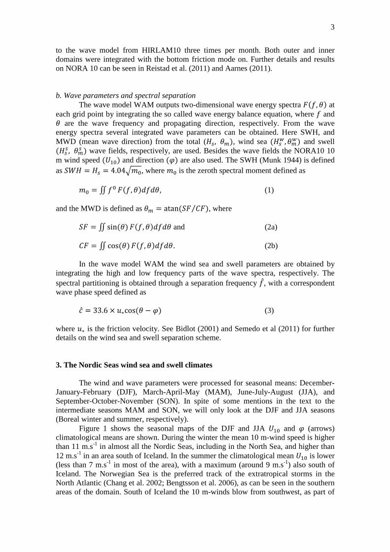
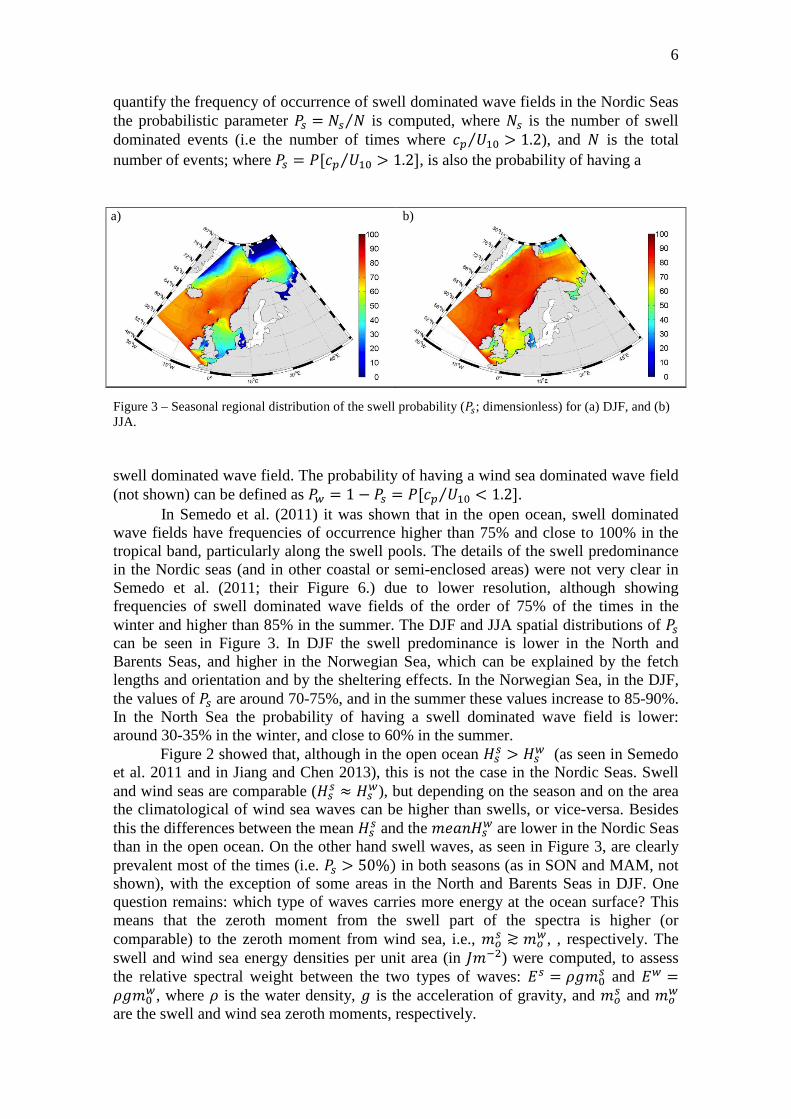
quantify the frequency of occurrence of swell dominated wave fields in the Nordic Seas the probabilistic parameter 𝑃𝑠 = 𝑁𝑠 𝑁⁄ is computed, where 𝑁𝑠 is the number of swell dominated events (i.e the number of times where 𝑐𝑝 𝑈10⁄ > 1.2), and 𝑁 is the total number of events; where 𝑃𝑠 = 𝑃[𝑐𝑝 𝑈10⁄ > 1.2], is also the probability of having a

a)

b)

Figure 3 – Seasonal regional distribution of the swell probability (𝑃𝑠; dimensionless) for (a) DJF, and (b) JJA. swell dominated wave field. The probability of having a wind sea dominated wave field (not shown) can be defined as 𝑃𝑤 = 1 − 𝑃𝑠 = 𝑃[𝑐𝑝 𝑈10⁄ < 1.2].

In Semedo et al. (2011) it was shown that in the open ocean, swell dominated wave fields have frequencies of occurrence higher than 75% and close to 100% in the tropical band, particularly along the swell pools. The details of the swell predominance in the Nordic seas (and in other coastal or semi-enclosed areas) were not very clear in Semedo et al. (2011; their Figure 6.) due to lower resolution, although showing frequencies of swell dominated wave fields of the order of 75% of the times in the winter and higher than 85% in the summer. The DJF and JJA spatial distributions of 𝑃𝑠 can be seen in Figure 3. In DJF the swell predominance is lower in the North and Barents Seas, and higher in the Norwegian Sea, which can be explained by the fetch lengths and orientation and by the sheltering effects. In the Norwegian Sea, in the DJF, the values of 𝑃𝑠 are around 70-75%, and in the summer these values increase to 85-90%. In the North Sea the probability of having a swell dominated wave field is lower: around 30-35% in the winter, and close to 60% in the summer.

Figure 2 showed that, although in the open ocean 𝐻𝑠𝑠 > 𝐻𝑠𝑤 (as seen in Semedo et al. 2011 and in Jiang and Chen 2013), this is not the case in the Nordic Seas. Swell and wind seas are comparable (𝐻𝑠𝑠 ≈ 𝐻𝑠𝑤), but depending on the season and on the area the climatological of wind sea waves can be higher than swells, or vice-versa. Besides this the differences between the mean 𝐻𝑠𝑠 and the 𝑚𝑒𝑎𝑛𝐻𝑠𝑤 are lower in the Nordic Seas than in the open ocean. On the other hand swell waves, as seen in Figure 3, are clearly prevalent most of the times (i.e. 𝑃𝑠 > 50%) in both seasons (as in SON and MAM, not shown), with the exception of some areas in the North and Barents Seas in DJF. One question remains: which type of waves carries more energy at the ocean surface? This means that the zeroth moment from the swell part of the spectra is higher (or comparable) to the zeroth moment from wind sea, i.e., 𝑚𝑜

𝑠 ≳ 𝑚𝑜𝑤, , respectively. The

swell and wind sea energy densities per unit area (in 𝐽𝑚−2) were computed, to assess the relative spectral weight between the two types of waves: 𝐸𝑠 = 𝜌𝑔𝑚0

𝑠 and 𝐸𝑤 =𝜌𝑔𝑚0

𝑤, where 𝜌 is the water density, 𝑔 is the acceleration of gravity, and 𝑚𝑜𝑠 and 𝑚𝑜

𝑤 are the swell and wind sea zeroth moments, respectively.

7

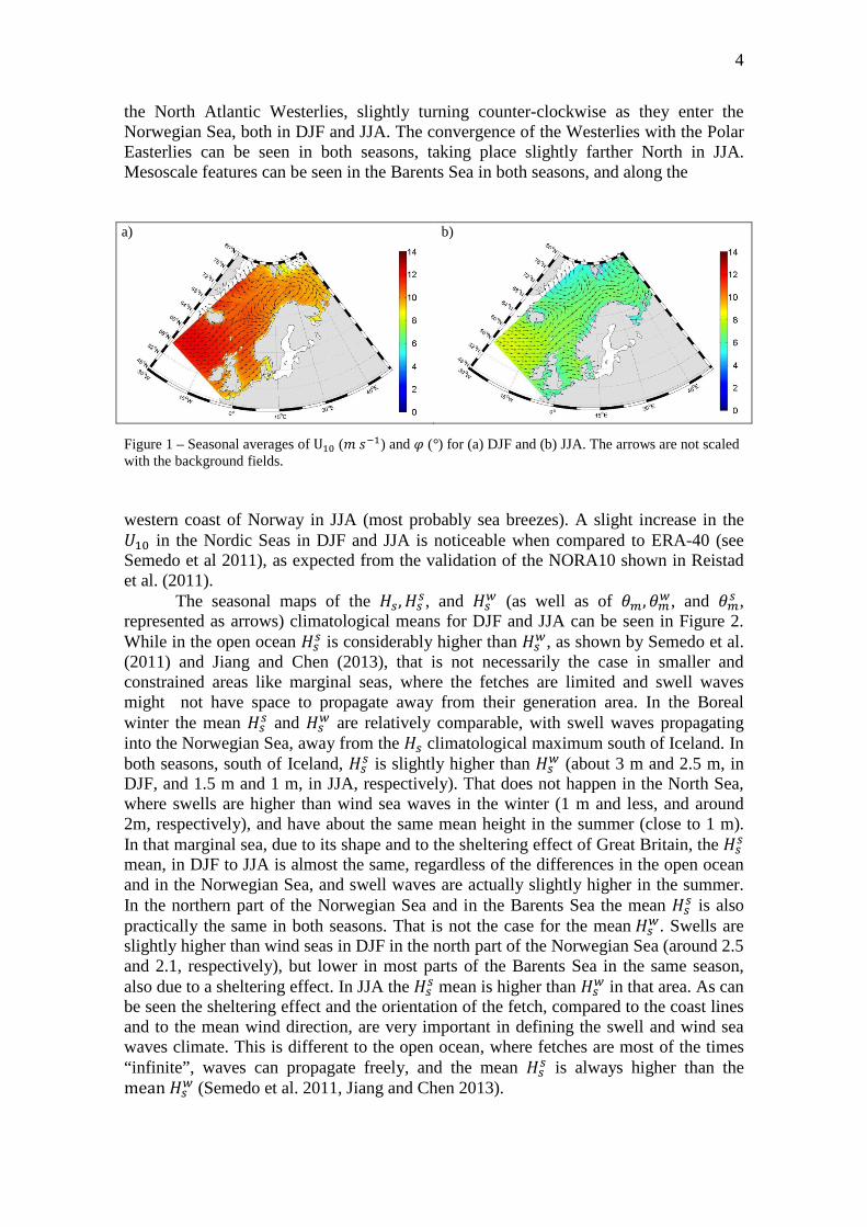
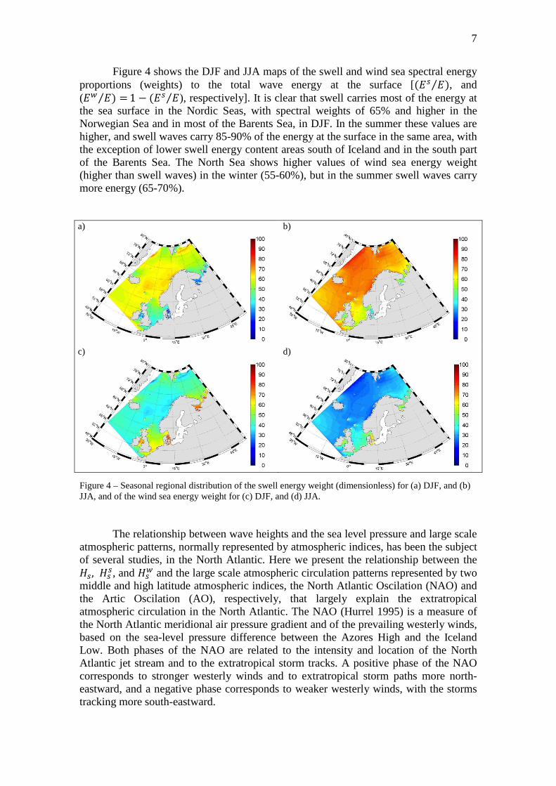
Figure 4 shows the DJF and JJA maps of the swell and wind sea spectral energy proportions (weights) to the total wave energy at the surface [(𝐸𝑠 𝐸⁄ ), and (𝐸𝑤 𝐸) =⁄ 1 − (𝐸𝑠 𝐸⁄ ), respectively]. It is clear that swell carries most of the energy at the sea surface in the Nordic Seas, with spectral weights of 65% and higher in the Norwegian Sea and in most of the Barents Sea, in DJF. In the summer these values are higher, and swell waves carry 85-90% of the energy at the surface in the same area, with the exception of lower swell energy content areas south of Iceland and in the south part of the Barents Sea. The North Sea shows higher values of wind sea energy weight (higher than swell waves) in the winter (55-60%), but in the summer swell waves carry more energy (65-70%). a)

b)

c)

d)

Figure 4 – Seasonal regional distribution of the swell energy weight (dimensionless) for (a) DJF, and (b) JJA, and of the wind sea energy weight for (c) DJF, and (d) JJA. The relationship between wave heights and the sea level pressure and large scale atmospheric patterns, normally represented by atmospheric indices, has been the subject of several studies, in the North Atlantic. Here we present the relationship between the 𝐻𝑠, 𝐻𝑠𝑠, and 𝐻𝑠𝑤 and the large scale atmospheric circulation patterns represented by two middle and high latitude atmospheric indices, the North Atlantic Oscilation (NAO) and the Artic Oscilation (AO), respectively, that largely explain the extratropical atmospheric circulation in the North Atlantic. The NAO (Hurrel 1995) is a measure of the North Atlantic meridional air pressure gradient and of the prevailing westerly winds, based on the sea-level pressure difference between the Azores High and the Iceland Low. Both phases of the NAO are related to the intensity and location of the North Atlantic jet stream and to the extratropical storm tracks. A positive phase of the NAO corresponds to stronger westerly winds and to extratropical storm paths more north-eastward, and a negative phase corresponds to weaker westerly winds, with the storms tracking more south-eastward.

8

The AO (or NAM – Northern Annular Mode) represents the opposing pattern of pressure between the Arctic Ocean and the northern middle latitudes. When the atmospheric pressure is low in the Arctic, it tends to be high in the northern middle latitudes (northern Europe and North America); if the atmospheric pressure is high in the middle latitudes it is often low in the Arctic. When pressure is low in the Arctic and high in middle latitudes, the AO is in its positive phase, and if the pattern is reversed the AO is said to be in its negative phase. The AO has an important effect on the weather in the high latitudes of the Northern Hemisphere: an AO in a positive is represents stronger westerlies and ocean storms tracking north; the pattern reverses when the AO is in a negative phase, and the stormy weather occurs in the more temperate regions of Europe and United States. a)

b)

c)

d)

e)

f)

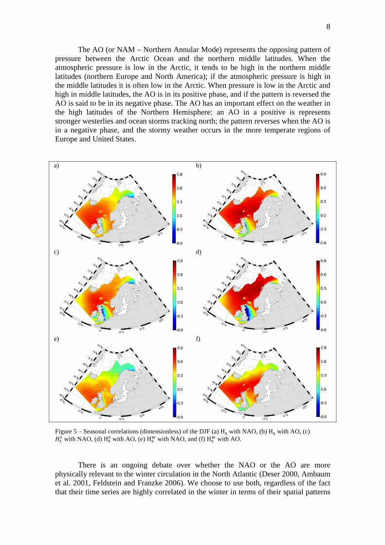
Figure 5 – Seasonal correlations (dimensionless) of the DJF (a) Hs with NAO, (b) Hs with AO, (c) 𝐻𝑠𝑠 with NAO, (d) Hs

s with AO, (e) Hsw with NAO, and (f) Hs

w with AO.

There is an ongoing debate over whether the NAO or the AO are more physically relevant to the winter circulation in the North Atlantic (Deser 2000, Ambaum et al. 2001, Feldstein and Franzke 2006). We choose to use both, regardless of the fact that their time series are highly correlated in the winter in terms of their spatial patterns

9

and their temporal evolution, because of the relation of the AO with higher latitude sea level pressure patterns, compared to the NAO. Wallace (2000) suggests that the NAO may be regarded as distinct from the AO only if the NAO is defined with a local station-based index, rather than from time-dependent projections on to a hemispheric field. Here we use the NAO index based on the normalized pressure difference between the Azores (Ponta Delgada) and Iceland (Reykjavik).

Figure 5 shows the DJF correlation coefficient maps (𝑟-correlation coefficient) between 𝐻𝑠,𝐻𝑠𝑠, and 𝐻𝑠𝑤 and the NAO and AO indices. The correlation values between 𝐻𝑠 and the NAO are high (𝑟 ≈ 0.8) near the west coast of Ireland, and relatively high (𝑟 ≳ 0.7) in a large area of the Norwegian Sea, but lower in the North Sea (𝑟 ≲ 0.5,

a)

b)

c)

d)

e)

f)

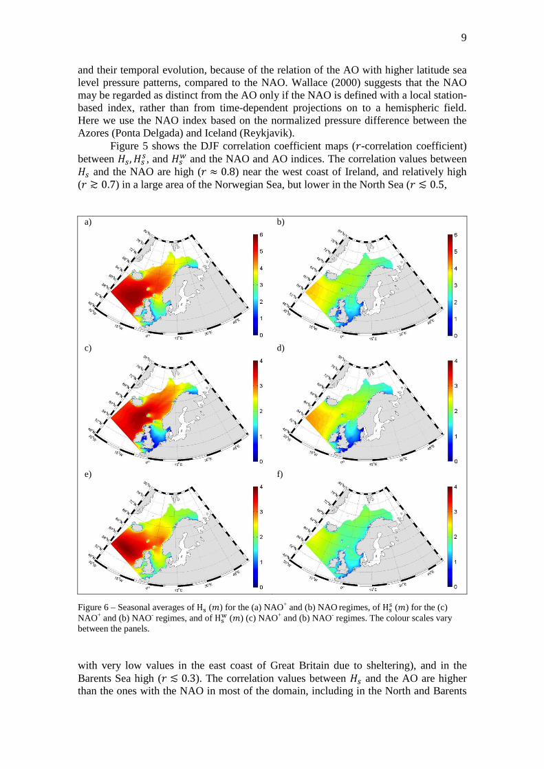
Figure 6 – Seasonal averages of Hs (𝑚) for the (a) NAO+ and (b) NAO regimes, of Hss (𝑚) for the (c)

NAO+ and (b) NAO- regimes, and of Hsw (𝑚) (c) NAO+ and (b) NAO- regimes. The colour scales vary

between the panels.

with very low values in the east coast of Great Britain due to sheltering), and in the Barents Sea high (𝑟 ≲ 0.3). The correlation values between 𝐻𝑠 and the AO are higher than the ones with the NAO in most of the domain, including in the North and Barents

10

Seas), and has a different pattern, with a large area of high correlation (𝑟 ≈ 0.9) between Iceland, Norway and Scotland.

The correlation between 𝐻𝑠𝑠, and 𝐻𝑠𝑤 and the NAO in DJF are relatively low (higher for 𝐻𝑠𝑠, with 𝑟 ≲ 0.65, with a strong sheltering effect in the North Sea, and with the higher correlation values for 𝐻𝑠𝑤 south of Iceland, 𝑟 ≲ 0.55, where the Westerlies blow strongest in DJF (see Figure 1 above). The higher correlation values of the swell wave heights in the north part of the Norwegian Sea and in the Barents Seas, along with the sheltering effect in the North Sea, can be seen as an indicator of waves generated more south that propagated north-westward. The correlation values between 𝐻𝑠𝑠, and 𝐻𝑠𝑤 and the AO are higher compared with the ones with the NAO. The high correlation values cover a larger area, in the case of swell wave heights (𝑟 ≈ 0.8 − 0.9), a great part of the Norwegian and Barents Seas.

a)

b)

c)

d)

e)

f)

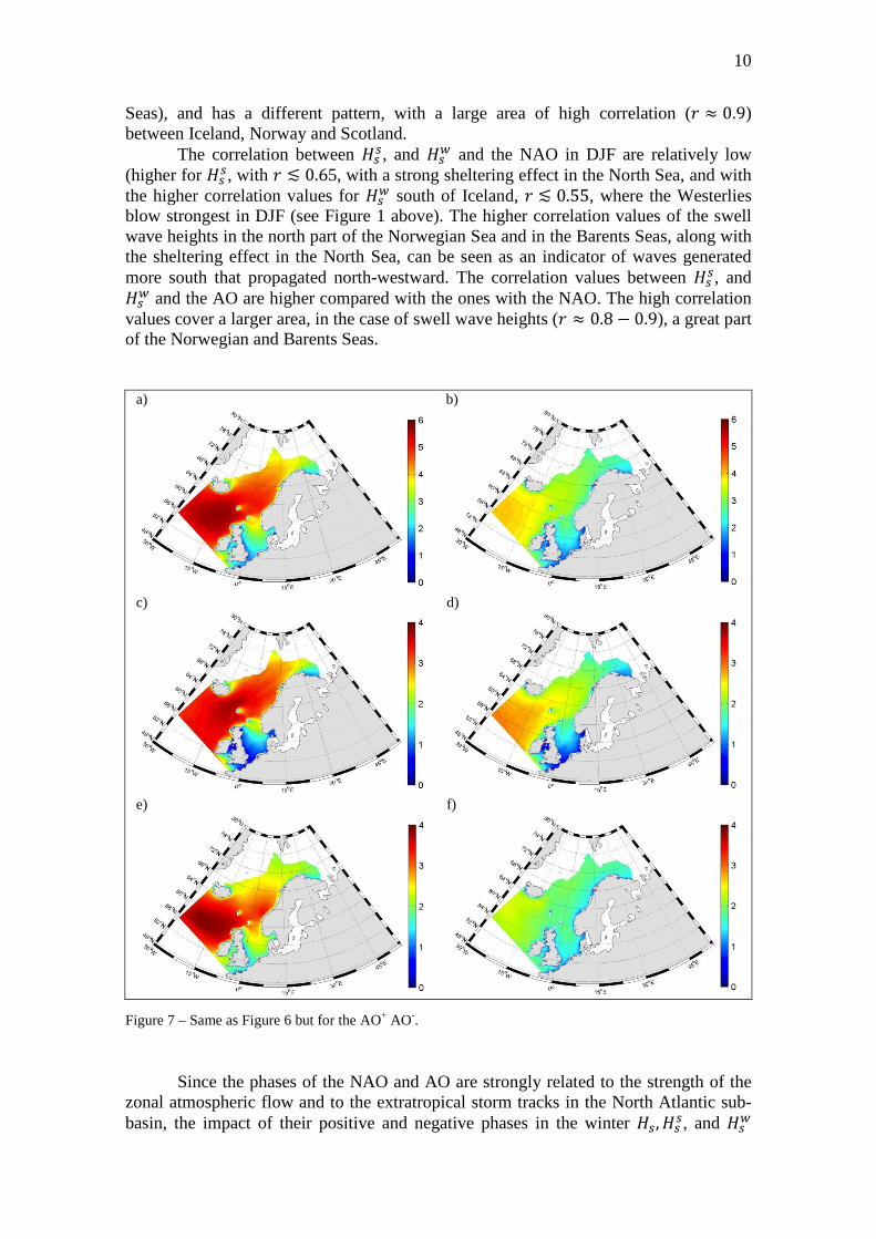
Figure 7 – Same as Figure 6 but for the AO+ AO-.

Since the phases of the NAO and AO are strongly related to the strength of the zonal atmospheric flow and to the extratropical storm tracks in the North Atlantic sub-basin, the impact of their positive and negative phases in the winter 𝐻𝑠,𝐻𝑠𝑠, and 𝐻𝑠𝑤

11

climates was investigated. The positive and negative phases of the atmospheric indices are hereafter designated as NAO+ and AO+, and NAO– and AO–, respectively. The seasonal maps of the DJF 𝐻𝑠,𝐻𝑠𝑠, and 𝐻𝑠𝑤 climatological means, separated for the NAO+ and NAO– (AO+ and AO–) regimes are shown in Figure 6 (Figure 7). The differences between the effects of the positive and negative regimes of the two indices on the wave heights in the North Atlantic are striking. The NAO+ and AO+ 𝐻𝑠,𝐻𝑠𝑠, and 𝐻𝑠𝑤 DJF means have a similar pattern, with the latter exhibiting a slight northward displacement of the climatological maxima. These patterns are also similar to the “total” means shown in Figure 2 above, with the wave height maxima in the NAO+ and AO+ regimes (for 𝐻𝑠,𝐻𝑠𝑠, and 𝐻𝑠𝑤) being more spatially constrained. The differences reside on the magnitudes of the wave heights in NAO+ and AO+ regimes compared to the total means, being ~1 m higher for 𝐻𝑠 and 𝐻𝑠𝑠, at the maxima, and more than 1 m for 𝐻𝑠𝑤. The swell dominance of the wave field (𝑃𝑠 pattern) for the NAO+ and AO+ (not shown) is now lower, as is the mean wind speed (also not shown) showing a higher predominance of locally generated waves. The 𝐻𝑠,𝐻𝑠𝑠, and 𝐻𝑠𝑤 DJF means for the negative phase show also similar patterns and magnitudes (between the NAO– and the AO– regimes), although the climatological maxima (partly outside the domain) seem to be more to the west for the NAO– regime DJF means. When compared to the NAO+ and AO+ regimes the magnitudes of the negative phase 𝐻𝑠 and 𝐻𝑠𝑠 DJF means are lower (~1.5-2 m for 𝐻𝑠, and ~1 m for 𝐻𝑠𝑠). The differences between the 𝐻𝑠𝑤 DJF means (positive and negative phases) are higher, with considerably lower locally generated wave heights (~2 m lower, representing a 50% decrease or more in most areas). The differences between the NAO– and AO– 𝐻𝑠, 𝐻𝑠𝑠, and 𝐻𝑠𝑤 seasonal means are also clear (higher, in percentage, than the differences in the NAO+ and AO+ regimes), with the negative phase seasonal mean wave heights being considerably lower. 4. Concluding remarks A qualitative analysis of the wave field in the Nordic Seas, based on the study of the wind sea and swell climatological characteristics, has been presented. The influence of the large scale atmospheric circulation patterns, represented by two atmospheric indices, the NAO and the AO, on the wind sea and swell regional climates has also been investigated. The high resolution regional wave reanalysis NORA10 allowed a better description of the wind sea and swell characteristics, compared to the previous study from Semedo et al. (2010), which was based on the ERA-40 reanalysis. It has been shown that the wind sea and swell characteristics in the Nordic Seas are different from the open ocean, where the mean 𝐻𝑠𝑠 is clearly higher than the mean 𝐻𝑠𝑤. This is not the case in the Nordic Seas, mainly in the North and Barents Sea, due to the sheltering effect and to the orientation of the fetch in relation to the coast lines and to the mean wind direction. In the winter, in some areas, the mean 𝐻𝑠𝑤 can be higher than the mean 𝐻𝑠𝑠. In spite of this, swell waves are clearly more prevalent in the area, and carry most of the energy at the ocean surface, although less than in the open ocean.

The impact of the storm tracks and of the strength of the zonal flow, here represented by the atmospheric indices NAO and AO, on the wind sea and swell wave heights is clear. These two indices are clearly correlated with the wave heights in the Nordic Seas, with the AO explaining more of the wave heights variability in higher latitudes. During the positive phase of the NAO or AO the mean 𝐻𝑠𝑤 is about the same or even higher than the mean 𝐻𝑠𝑠 in most of the Nordic Seas, particularly in the North

12

and Barents Seas. When storms track more south, and the NAO and AO are in their negative phase that is not completely the case: the mean 𝐻𝑠𝑠 now clearly higher than the mean 𝐻𝑠𝑤 in the Norwegian Sea, but in the sheltered North and Barents Seas the wind sea waves are still higher. Acknowledgements The Norwegian Deepwater Programme (NDP) financed the construction of the NORA10 hindcast archive.

REFERENCES Alves, J.H.G.M, M.L. Banner, and I.R. Young, 2003: Revisiting the Pierson-Moskowitz Asymptotic Limits for Fully Developed Wind Waves. J. Phys. Oceanogr., 33, 1301-1323. Alves, J. H.G.M., 2006: Numerical Modeling of Ocean Swell Contributions to the Global Wind-Wave Climate. Ocean Model., 11, 98-122. Ambaum, M.H.P., B.J. Hoskins, and D.B. Stephenson, 2001: Arctic Oscillation or North Atlantic Oscillation? J. Climate, 14, 3495-3507. Aarnes, O.J., Ø. Breivik & M. Reistad, 2012. Wave Extremes in the Northeast Atlantic. J. Climate, 25, 1529–1543. Bengtsson, L., K. Hodges, and E. Roeckner, 2006: Storm tracks and climate change, J. Climate, 19, 3518-3543. Bidlot, J.-R., 2001: ECMWF wave model products. ECMWF Newsletter, No.91, ECMWF, Reading, United Kingdom, 9–15. Chang, E.K.M., S. Lee, and K.L. Swanson, 2002: Storm Track Dynamics. J Climate, 15, 2163-2183. Charnock, H., 1955: Wind Stress on a Water Surface. Q. J. R. Meteorol. Soc., 81, 639-640. Charnock, H., 1958: A Note on Empirical Wind-Wave Formulae. Q. J. R. Meteorol. Soc., 84, 443-447. Chen, G., B. Chapron, R. Ezraty, and D. Vandemark, 2002: A Global View of Swell and Wind Sea Climate in the Ocean by Satellite Altimeter and Scatterometer. J. Atmos. Oceanic Technol., 19, 1849-1859. Csanady, G.T. 2001: Air-Sea Interaction: Laws and Mechanisms. Cambridge, UK: Cambridge Univ. Press, 237 pp. Desjardin, S. J. Mailhot, R. Lalbeharry, 2000: Examination of the Impact of a Coupled Atmospheric and Ocean wave System. Part I: Atmospheric aspects. – J. Phys.Oceanogr. 30, 385–401.

13

Deser, C., 2000: On the Teleconnectivity of the “Arctic Oscillation”. Geophys. Res. Lett., 27, 779-782. Doyle, J.D., 1995: Coupled ocean wave/atmosphere mesoscale model simulations of cyclogenesis. Tellus, 47A, 766–788. Feldstein, Steven B., Christian Franzke, 2006: Are the North Atlantic Oscillation and the Northern Annular Mode Distinguishable? J. Atmos. Sci., 63, 2915-2930. Gulev, S.K., and V. Grigorieva, 2006: Variability of the Winter Wind Waves and Swell in the North Atlantic and North Pacific as Revealed by the Voluntary Observing Ship Data. J. Climate, 19, 5667-5685. Hurrell, J.W., 1995: Decadal trends in the North Atlantic Oscillation and Relationships to Regional Temperature and Precipitation. Science, 269, 676-679. Hoögström, U., A. Smedman, E. Sahlée, W.M. Drennan, K.K. Kahma, H. Pettersson, and F. Zhang, 2009: The Atmospheric Boundary Layer During Swell: A Field Study and Interpretation of the Turbulent Kinetic Energy Budget for High Wave Ages. J. Atmos. Sci., 66, 2764–2779. Holthuijsen, L. H., 2007: Waves in Oceanic and Coastal Waters. Cambridge University Press, 387 pp. Janssen, P.A.E.M., P. Viterbo, 1996: Ocean waves and the atmospheric climate. – J. Climate 9, 1269–1287. Jiang, H., G. Chen, 2013: A Global View on the Swell and Wind Sea Climate by the Jason-1 Mission: A Revisit. J. Atmos. Oceanic Technol., 30, 1833-1841. Lionello, P., P. Malguzzi, A. Buzzi, 1998: Coupling between the Atmospheric Circulation and the Ocean Wave Field: An Idealized Case. J. Phys. Ocean. 28, 161–177. Komen, G.J., L. Cavaleri, M. Donelan, K. Hasselmann, S. Hasselmann and P.A.E.M. Janssen, 1994: Dynamics and Modelling of Ocean Waves. Cambridge Univ. Press, Cambridge, UK, 560 pages. Kinsman, B., 1965: Wind Waves. Prentice-Hall, Englewood Cliffs, NJ, p. 676. Munk, W. H., 1944: Proposed Uniform Procedure for Observing Waves and Interpreting Instrument Records. Scripps Institution of Oceanography, Wave Project Rep. 26, 22 pp. Pierson, W. J., and L. Moskowitz, 1964: A Proposed Spectral Form for Fully Developed Wind Seas Based on the Similarity Theory of S. A. Kitaigorodskii. J. Geophys. Res., 69, 5181–5190.

14

Reistad,M.,O. Breivik, H.Haakenstad, O. J. Aarnes & B. R. Furevik, 2011. A high-resolution hindcast of wind and waves for the North Sea, the Norwegian Sea and the Barents Sea. J. Geophys. Res., 116, C05019. Semedo, A., Ø. Sætra, A. Rutgersson, K. Kahma, and H. Pettersson, 2009: Wave-Induced Wind in the Marine Boundary Layer. J. Atmos. Sci., 66, 2256–2271. Semedo, A.,,K. Sušelj, A. Rutgersson, A. Sterl, 2011: A Global view on the wind sea and swell climate and variability from ERA-40. J. Climate, 24, 5, 1461-1479 Smith, S. D., and Coauthors, 1992: Sea surface wind stress and drag coefficients: The HEXOS results. Bound.-Layer Meteor., 60, 109–142. Snodgrass, F.E., Groves, G.W., Hasselmann, K.F., Miller, G.R., Munk, W.H., Powers, W.M. 1966: Propagation of swell across the Pacific. Philos. Trans. R. Soc. London A259, 431–497. Undén, P., & Coauthors, 2002. HIRLAM-5 scientific documentation. HIRLAM-5 Project, SMHI Tech. Rep. S-601 76, 144 pp. Uppala, S. M., & Coauthors, 2005. The ERA-40 Re-Analysis. Quart. J. Roy. Meteor. Soc., 131, 2961–3012. Wallace, J. M., 2000: North Atlantic Oscillation/Annular Mode: Two paradigms–one phenomenon. Quart. J. Roy. Meteor. Soc., 126, 791–805. WAMDI Group, 1988: The WAM model – A third generation ocean wave prediction model. J. Phys. Oceanogr., 18, 1775–1810. Weisse, R. and H. Günther, 2007: Wave climate and long-term changes for the Southern North Sea obtained from a high-resolution hindcast 1958-2002, Ocean Dynamics, 57, 161-172.