Embed Size (px)
Citation preview
WIND TUNNEL BLOCKAGE CORRECTIONS:
A COMPUTATIONAL STUDY
by
DEEPAK SAHINI, B.Tech.
A THESIS
IN
MECHANICAL ENGINEERING
Submitted to the Graduate Faculty of Texas Tech University in
Partial Fulfillment of the Requirements for
the Degree of
MASTER OF SCIENCE
IN
MECHANICAL ENGINEERING
Approved
Chairperson of the Committee
Accepted
Dean of the Graduate School
August, 2004

AC^KNOWLI'DGMENTS
1 consider this as a pri\ilege to thank the people who have made this thesis
possible.
1 would like to sincerely thank my advisor. Dr. Siva Parameswaran for his
support, encouragement, and assistance during my work. He, constantly monitored my
progress and provided me \\ ith a great deal of ideas throughout my thesis work.
I thank Dr. Darryl L. James and Dr. Padmanabhan Seshaiyer for serving on my
committee. I appreciate the help and assistance from my colleagues. Dr. Senthooran
Sivapalan and Dr. Dong Dae Lee. I thank the Department of Mechanical Engineering for
the excellent CFD lab facility. I also appreciate the services rendered by the Texas Tech
Library for providing assistance with the necessary literature.
Now, I take the opportunity and pride of thanking my father Balagangadhar Tilak
Sahini, mother Jayalakshmi Sahini and my sister Shilpa Rekha Sahini, without whose
support and motivation this achievement of mine, would not have been possible. Last but
not least, I thank my roommates and friends, Venkata Suman Mowa, Seethapathi Rao
Latchireddi, Sandeep Singh Thakur, Anil Kumar Chandolu, Ravi Sekhar Gunda, Niranjan
Das Mettu, Pavan Chintapanti, Ram Prashant Nellore and Kishore Kumar Gali for their
valuable suggestions, encouragement and cooperation during all times.
11
lABLE OF CONTENTS
.ACKNOWLEDGMENTS ii
ABSTRACT v
LIST OF TABLES vi
LIST OF FIGURES vii
NOMENCL.-\TURE xii
CH.APTER
1 INTRODUCTION 1
2 BACKGROUND WORK AND LITERATURE REVIEW 5
2.1 Wmd timnel Testing and Blockage Corrections 5
2.1.1 An Introduction to Wind Tunnel and its General Layout 5
2.1.2 Wind Tunnel Blockage Corrections 8
2.1.3 Basic Mechanism associated with Blockage Effects 9
2.1.4 Role of CFD in Wind Turmel Blockage Corrections 11
2.2 Literature Review 12
2.2.1 Review of work on Experimental determination of Blockage Correction 12
2.2.2 Review of work on Computational determination of
Blockage Correction 16
3 COMPUTATIONAL METHODOLOGY 21
3.1 Assumptions 22
3.2 Computational Setup and Solution Procedure 22
HI
3.2.1 Domain layout Considerations 22
3.2.2 Mesh General ion 27
3.2.3 Boundary and Initial Conditions 39
3.2.4 Turbulence Models and Numerical Methods 45
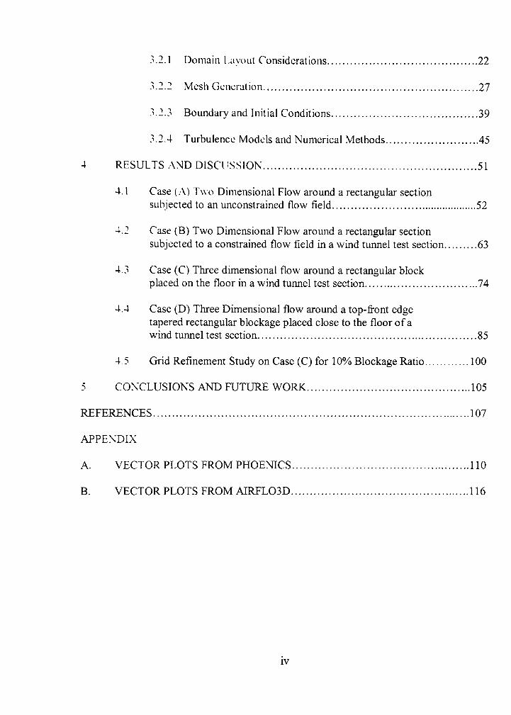
4 RESULTS .\ND DISCUSSION 51
4.1 Case (.\) T\\o Dimensional Flow around a rectangular section subjected to an unconstrained flow field 52
4.2 Case (B) Two Dimensional Flow around a rectangular section subjected to a constrained flow field in a wind tunnel test section 63
4.3 Case (C) Three dimensional flow around a rectangular block placed on the floor in a wind tunnel test section 74
4.4 Case (D) Three Dimensional flow around a top-front edge tapered rectangular blockage placed close to the floor of a wind tunnel test section 85
4.5 Grid Refinement Study on Case (C) for 10% Blockage Ratio 100
5 CONCLUSIONS AND FUTURE WORK 105
REFERENCES 107
APPENDIX
A. VECTOR PLOTS FROM PHOENICS 110
B. VECTOR PLOTS FROM AIRFL03D 116
IV
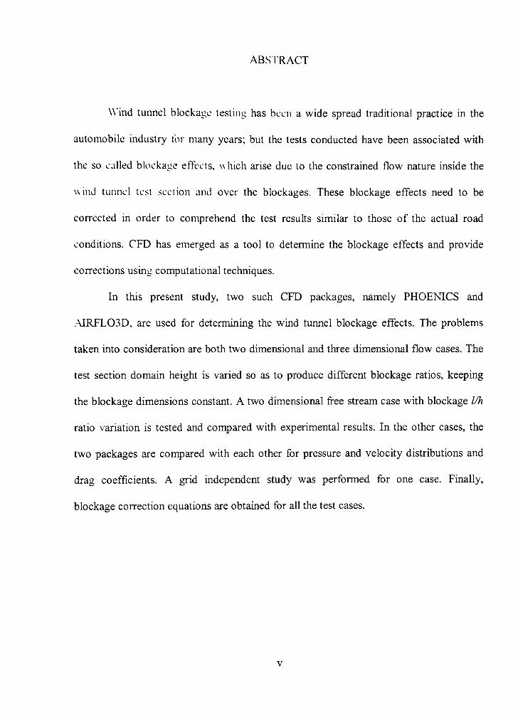
ABSfRACT
Wind tunnel blockage testing has been a wide spread traditional practice in the
automobile industry for many years; but the tests conducted have been associated with
the so called blockage effects, w hich arise due to the constrained flow nature inside the
wind tunnel test section and over the blockages. These blockage effects need to be
corrected in order to comprehend the test results similar to those of the actual road
conditions. CFD has emerged as a tool to determine the blockage effects and provide
corrections using computational techniques.
In this present study, two such CFD packages, namely PHOENICS and
.AIRFL03D, are used for determining the wind tunnel blockage effects. The problems
taken into consideration are both two dimensional and three dimensional flow cases. The
test section domain height is varied so as to produce different blockage ratios, keeping
the blockage dimensions constant. A two dimensional free stream case with blockage l/h
ratio variation is tested and compared with experimental results. In the other cases, the
two packages are compared with each other for pressure and velocity distributions and
drag coefficients. A grid independent study was performed for one case. Finally,
blockage correction equations are obtained for all the test cases.
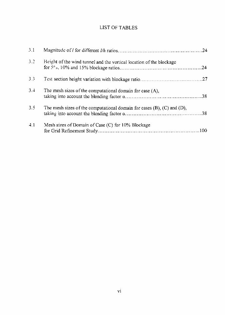
LIST OF TABLES
3.1 Magnitude of/ for different l/h ratios 24
3.2 Height ofthe wind tunnel and the vertical location ofthe blockage
for5\, . 10% and 15% blockage ratios 24
3.3 Test section height variation with blockage ratio 27
3.4 The mesh sizes ofthe computational domain for case (A), taking into account the blending factor a 38
3.5 The mesh sizes ofthe computational domain for cases (B), (C) and (D), taking into account the blending factor a 38
4.1 Mesh sizes of Domain of Case (C) for 10% Blockage for Grid Refmement Study 100
VI
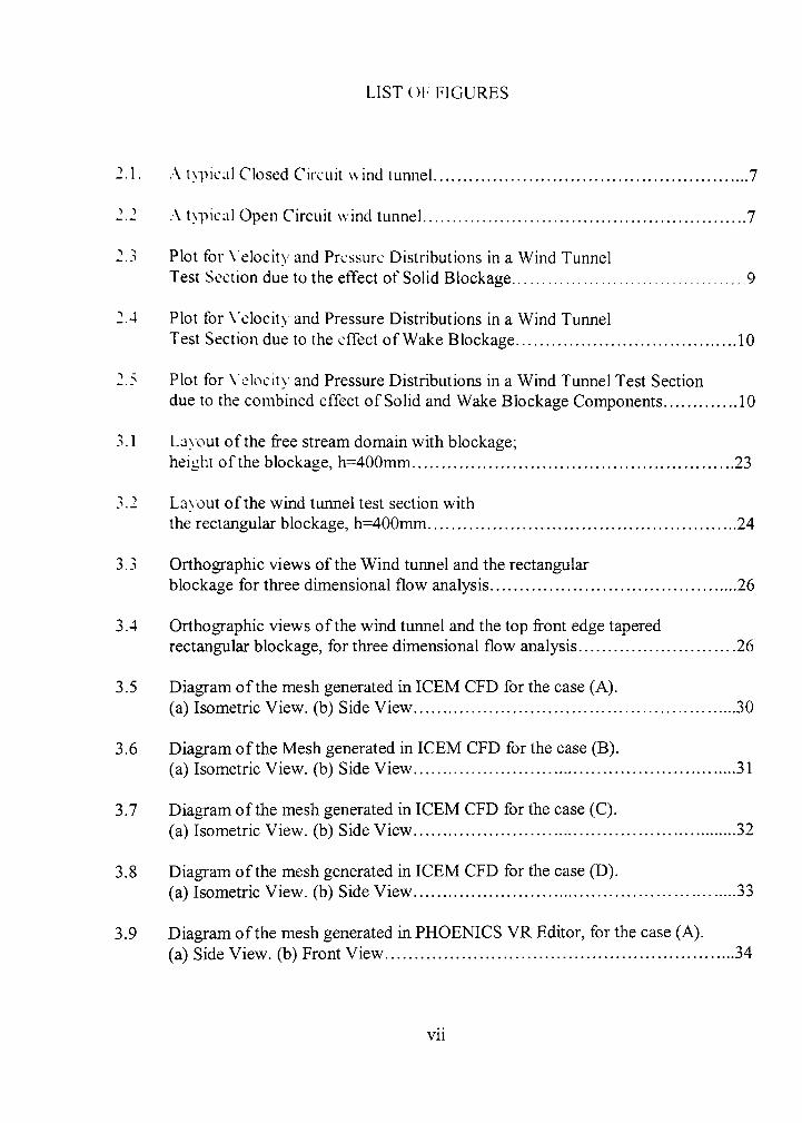
LIST Of FIGURES
2.1. .\ t\pical Closed Circuit wind tunnel 7
2.2 .\ typical Open Circuit wind tunnel 7
2.3 Plot for \elocity and Pressure Distributions in a Wind Tunnel Test Section due to the effect of Solid Blockage 9
2.4 Plot for X'elocity and Pressure Distributions in a Wind Tunnel Test Section due to the effect of Wake Blockage 10
2.5 Plot for X'elocity and Pressure Distributions in a Wind Tunnel Test Section due to the combined effect of Solid and Wake Blockage Components 10
3.1 Layout ofthe free stream domain with blockage; height of the blockage, h=400mm 23
3.2 Layout ofthe wind tunnel test section with the rectangular blockage, h=400nim 24
3.3 Orthographic views ofthe Wind tunnel and the rectangular blockage for three dimensional flow analysis 26
3.4 Orthographic views ofthe wind tunnel and the top front edge tapered rectangular blockage, for three dimensional flow analysis 26
3.5 Diagram ofthe mesh generated in ICEM CFD for the case (A). (a) Isometric View, (b) Side View 30
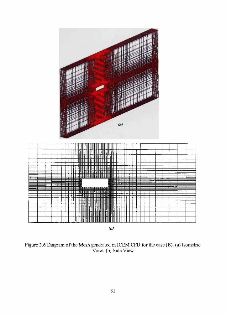
3.6 Diagram ofthe Mesh generated in ICEM CFD for the case (B). (a) Isometric View, (b) Side View 31
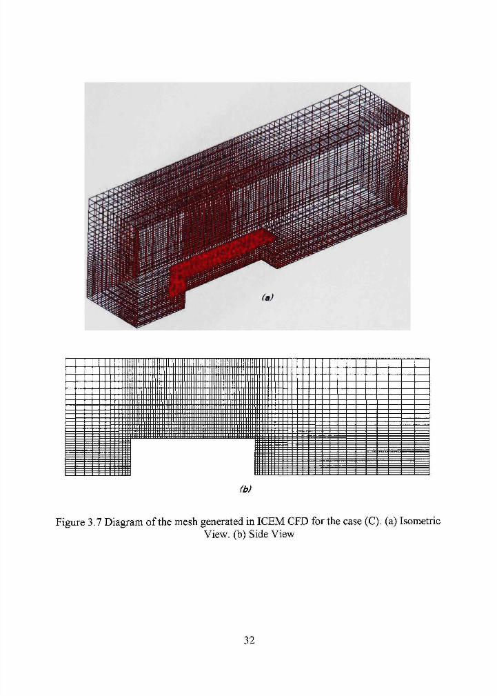
3.7 Diagram ofthe mesh generated in ICEM CFD for the case (C). (a) Isometric View, (b) Side View 32
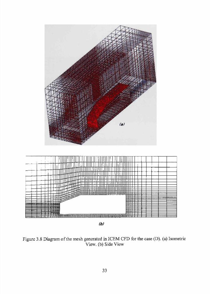
3.8 Diagram ofthe mesh generated in ICEM CFD for the case (D). (a) Isometric View, (b) Side View 33
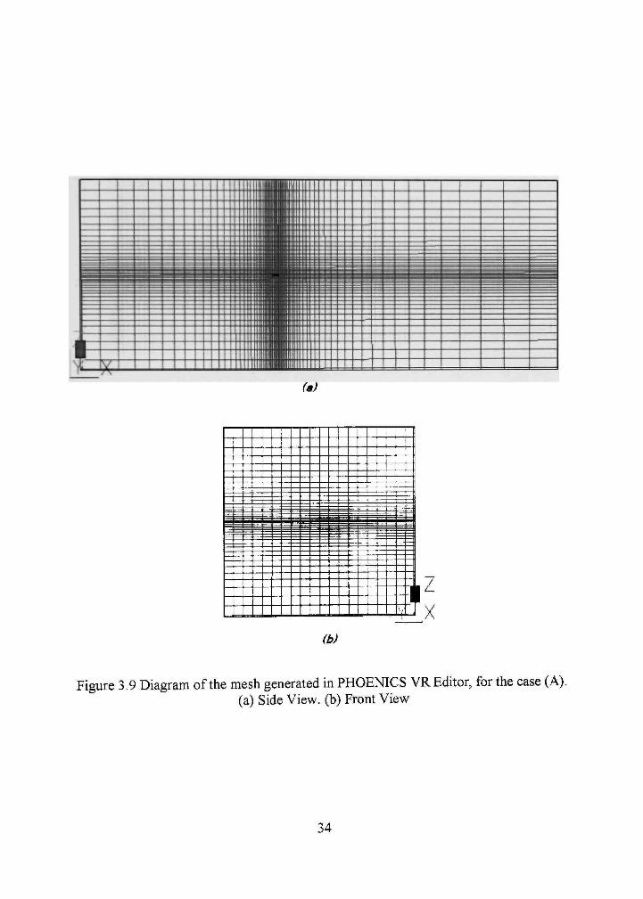
3.9 Diagram ofthe mesh generated in PHOENICS VR Editor, for the case (A). (a) Side View, (b) Front View 34
vu
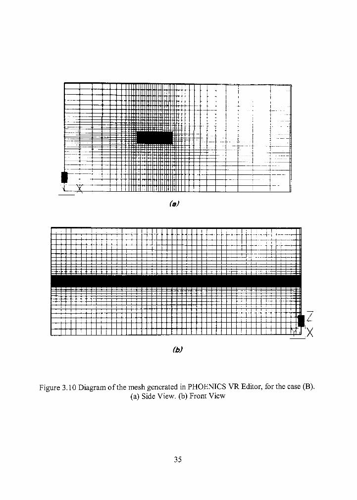
3.10 Diagram ofthe mesh generated in PHOENICS VR Editor, for the case (B). (a) Side \'lew . (b) Front View 35
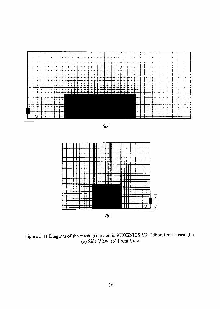
3.11 Diagram ofthe mesh generated in PHOENICS VR Editor, for the case (C). (a) Side N'iew. (b) Front View 36
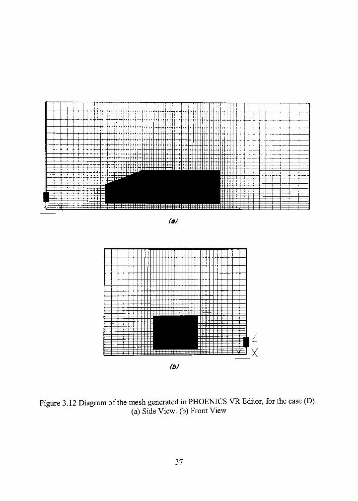
3.12 Diagram ofthe mesh generated in PHOENICS VR Editor, for the case (D). (a) Side X'iew. (b) Front View 37
3 13 Boundary conditions used in ICEM CFD for flow in case (A). (a) Side \iew. (b) Front View 39
3.14 Boundary conditions used in ICEM CFD for flow in case (B). (a) Side \'iew. (b) Front View 40
3.15 Boundary conditions used in PHOENICS for flow in cases (A) and (B). (a) Side \'iew. (b) Front View 41
3.16 Boundary conditions used in ICEM CFD for flow in case (C). (a) Side View, (b) Front View 42
3.17 Boundary conditions used in PHOENICS for flow in case (C). (a) Side View, (b) Front View 43
3.18 Boundary conditions used in ICEM CFD for flow in case (D). (a) Side View, (b) Front View 44
3.19 Boundary conditions used in PHOENICS for flow ia case (D). (a) Side View, (b) Front View 45
4.1 Line along which the Pressure and Velocity Distributions
are obtained in Two Dimensional case 52
4.2 Plot for Pressure Signature using PHOENICS data for Case (A) 54
4.3 Plot for Velocity Profile using PHOENICS data for Case (A) 55
4.4 Plot for Drag variation with l/h ratio using Experimental data for Case (A) 57
4.5 Plot for Drag variation with l/h ratio using PHOENICS data for Case (A) 58
4.6 Plot for Drag variation with l/h ratio using AIRFL03D data for Case (A) 59
4.7 Plot for Drag Correction using PHOENICS data for Case (A) 60
Vll l
4.S Plot for Drag Correction using A1RFL03D data for Case (A) 61
4.9 Plot for Pressure Signature using PHOENICS data for Case (B) 65
4.10 Plot for Velocity Profile using PHOENICS data for Case (B) 66
4.11 Plot for Pressure Signature using A1RFL03D data for Case (B) 67
4.12 Plot for Velocity Profile using A1RFL03D data for Case (B) 68
4.13 Plot for Drag Coefficient \ ariation with blockage ratio using PHOENICS data..71
4.14 Plot for Drag Coefficient variation with blockage ratio using AIRFL03D data..72
4.15 Plot for Drag Correction using AIRFL03D and PHOENICS data for Case (B)..73
4.16 Line along which the Pressure and Velocity Distributions
are obtained in case of Three Dimensional rectangular block 74
4.17 Plot for Pressure Signature using PHOENICS data for Case (C) 77
4.18 Plot for X'elocity Profile using PHOENICS data for Case (C) 78
4 19 Plot for Pressure Signature using AIRFL03D data for Case (C) 79
4.20 Plot for Velocity Profile using AIRFL03D data for Case (C) 80
4.21 Plot for Drag Coefficient varying with Blockage Ratio using PHOENICS data..83
4.22 Plot for Drag Coefficient varying with Blockage Ratio using AIRFL03D data..84
4.23 Lines along which the Pressure and Velocity Distributions are obtained in case of Three Dimensional top-edge tapered block 85
4.24 Plot for Pressure Signature at the top ofthe blockage, using PHOENICS data for Case (D) 88
4.25 Plot for Velocity Profile at the top ofthe blockage, using PHOENICS data for Case (D) 89
4.26 Plot for Pressure Signature at the top ofthe blockage, using AIRFL03D data for Case (D) 90
IX
4.27 Plot tor Velocity Profile at the top ofthe blockage, using AIRFL03D data for Case (D) ? 91
4.28 Plot for Pressure Signature at the bottom ofthe blockage, using PHOENICS data forC\ise(D) 93
4.20 Plot for \ elocity Profile at the bottom ofthe blockage, using PHOENICS data tor Case (D) 94
4.30 Plot for Pressure Signature at the bottom ofthe blockage, using .A1RFL03D data for Case (D) 95
4.31 Plot for X'elocity Profile at the bottom ofthe blockage, using AIRFL03D data for Case (D) 96
4.32 Plot for Drag Coefficient variation with Blockage Ratio using PHOENICS data 98
4.33 Plot for Drag Coefficient variation with Blockage Ratio using AIRFL03D data 99
4.34 Plot for variation of Pressure Signature with Mesh Refinement using PHOENICS Data 101
4.35 Plot for variation of Velocity Profile with Mesh Refmement using PHOENICS Data 102
4.36 Plot for variation of Pressure Signature with Mesh Refinement using AIRFL03D Data 103
4.37 Plot for variation of Velocity Profile with Mesh Refinement
using AIRFL03D Data 104
A. 1 Two dimensional rectangular block; 5% Blockage ratio 110
A.2 Two dimensional rectangular block; 10%) Blockage ratio I l l
A.3 Two dimensional rectangular block; 15% Blockage ratio I l l
A.4 Three dimensional rectangular block; 5% Blockage ratio 112
A.5 Three dimensional rectangular block; 10% Blockage ratio 113
A.6 Three dimensional rectangular block; 15% Blockage ratio 113
.\.7 Three dimensional top-front edge tapered block; 5% Blockage ratio 114
.A,.8 Three dimensional top-front edge tapered block; 5% Blockage ratio 115
.\.9 Three dimensional top-front edge tapered block; 15% Blockage ratio 115
B.l Two dimensional rectangular block; 5"/(i Blockage ratio 116
B.2 Two dimensional rectangular block; 10% Blockage ratio 117
B.3 Two dimensional rectangular block; 15% Blockage ratio 117
B.4 Three dimensional rectangular block; 5% Blockage ratio 118
B.5 Three dimensional rectangular block; 10%) Blockage ratio 119
B.6 Three dimensional rectangular block; 15% Blockage ratio 119
B.7 Three dimensional rectangular block; 15% Blockage ratio 120
B.8 Three dimensional top-front edge tapered block; 10% Blockage ratio 121
B.9 Three dimensional top-front edge tapered block; 15% Blockage ratio 121
XI

NOMENCLATURE
.-1 Projected area of cross section
--!,„ Area of cross section of blockage
-i, Area of cross section of wind tunnel
Ci, C:. Cfi Model constants of K-e model
Cjj,C(j Drag coefficient
C , Corrected drag coefficient
AC^ Change in drag coefficient
Cp Pressiu-e coefficient
Dfyg Distance between the NEP and the base of vehicle windshield
h Height ofthe blockage placed in the wind tunnel
H Height ofthe wind tunnel / the height ofthe free stream domain considered
k Distance from the nozzle exit point to the blockage
K Kinetic Energy ofthe fluid
/ Length ofthe blockage placed in the wind tunnel
L Length ofthe wind tunnel
NEP Nozzle exit point
P Mean pressure
Pi Instantaneous pressure
P/, Production of turbulence kinetic energy
q Reference dynamic pressure
xii
(/ Corrected reference dynamic pressure
t Time
u Inlet \elocitv
Instantaneous velocity in i' direction
Fluctuating \elocity in i'' direction
U- Xlean \ elocity in i'" direction
r. Magnitude of \ elocity at the edge
V^ Magnitude of reference velocity
w Width ofthe blockage placed in the wind tunnel
]]' W'idthof the wind timnel
A'. Y,Z Cartesian coordinates
Vn Yap correction
a Blending factor
8 Dissipation ofthe fluid
^ Blockage ratio in a two dimensional wind tunnel
// Dynamic viscosity
V, Eddy viscosity
p Density of fluid
I// Blockage correction factor
(^^ SoUd blockage correction factor
i//^ Wake blockage correction factor
xiii
¥, Blockage factor based on \ehicle frontal velocity profile
.X Shape factor
Z Mesh si/e
xiv
CHAPTl'R 1
INTRODUCTION
.-Xerodyiiamics is the physics of motion of gases. The study of this field had
gained significance with the ad\ent ofthe aircraft. Its primary concern was to determine
the flow of air around the body (airplane), predict the forces and moments acting on it
and to minimize the aerod\Tiamic drag; thus, increasing the performance of flight. Soon
after this, aerodynamics was extended to automobiles, stmctures, and environmental
studies. Of these, aerodynamics applied to automobiles has gained popularity very
quickly as a result ofthe development in the motor industry.
In the Early stages of vehicle research, the main concentration was on design and
improvement of the components, aesthetics and spatial manipulation. The desire for
higher driving speed vehicles for faster modes of road transportation was the main reason
for applying aerodynamics in the field of transportation technology. It was because of
the fact that, at high speeds, the performance of the engine also depended on the
aerodynamic drag caused by the air flow around the vehicle; thus this new branch of
vehicle aerodynamics has emerged. The initial development stressed on reducing the
aerodynamic drag. This has fascinated aerodynamicists, vehicle designers, and stylists to
bring about novel designs and test various body shapes. This has revolutionized the
development of vehicle technology. Further, the field was extended to flow of air through
the body and flow process within the machinery.

Xlany similarities exist between the primary purposes of research in aerodynamics
of motor vehicles and that of aircraft, such as lowering aerodynamic drag and balancing
of tbrces and moments for directional stability. However, they differ in many significant
aspects. The analysis of aeiod\namic eflbcts on automobiles are mostly done
experimentally, unlike those on aircrafts that are, to a great extent, proposed theoretically,
followed b\ experimentation on scaled models in wind tunnels. The evolution ofthe car-
shape is the result of aerodynamic developments carried out by car makers in their
specific purpose wind tunnels. On the other hand, aerodynamic development of road
vehicles invohes high expenditure.
The capital required for setting up of testing facilities, such as wind tunnels and
climatic tunnels pro\ed to be very high. The experiments conducted were not time
effectix e. The quaUty and the reliability ofthe results intended, increased the demand for
the quality of the wind tunnel and thereby increased the developmental costs steeply.
Results published in literature, when properly apphed, would have eliminated wind
tunnel testing to some extent; but lower drag coefficients could have been achieved only
at the expense of high cost, time, and painstaking process of preparing the fiiU-scale
model and then conducting tests on it. Scaled model test results were subjected to
numerous doubts associated with realistic simulation of Reynolds number, surface and
underbody details, engine cooling and passenger compartment flows, tunnel wall
boundary layer and model support interference effects and effects of flow-intmsive
probes. On top of all these, the basic and most important wind tunnel experimental

I'actors that are needed to be taken care of, are the blockage effects. These blockage
effects account for drag variation compared to the actual road testing.
In order to overcome some ofthe problems associated with wind tunnel testing,
experts and researchers initiated the development of flow simulations using computers, in
the early se\'enties. Many mathematical techniques and models have been developed so
far to provide better and cfTicient algorithms related to the flow simulations.
Computational Fluid Dynamics (CFD) has emerged as one such tool in aerodynamic
development of motor vehicles. Recent advances in computing techniques have proved to
haxe reduced the cost and time of analysis, considerably. The following are the
ad\ antages of using CFD over wind turmels:
1. Can be cheap and quick, due to the high computation speeds of modem computer
2. Detailed information in both space and time is obtained
3. Empirical input need not be used
4. Xo scahng effects are required
5. Analysis can be done on wide range of shapes
6. It can be used for vaUdating the wind tunnel test results
Tremendous research has been done experimentally to determine the blockage
effects of the blockage placed in the wind tunnel test section by the Motor Industry
Research Association (MIRA), College of Aeronautics (CoA), National Research
Council of Canada (NRCC), and many others. The experimental results have been
documented by the SAE International. The aim of this present work is, to undertake test
cases of simple blockages placed in a virtual wind tunnel test section, created using CAD
modeling software. Initially, a simple two dimensional rectangular block under
unconstrained free stream condition is considered and drag behavior curve for different
///) (LengthHeight) ratios is determined, in order to gain confidence of the CFD
experiments being performed in the present study. The computational results are
compared with those ofthe experimental characteristics and drag correction equation is
detemiined.
The computational study is extended to simple two dimensional and three
dimensional blockages subjected to constrained flow inside wind tunnel test sections. The
blockage ratio is varied, keeping the same blockage dimensions and increasing the height
ofthe wind turmel test section. The flow parameter profiles and the drag created by the
blockage for different blockage ratios are determined using the CFD codes, AIRFL03D,
and PHOENICS. The blockage correction equations are determined. These blockage
correction equations can be applied for other cases and the corrected aerodynamic
coefficients can be determined. A grid independent study has been performed to
determine the effect of computational grid size on the flow parameters.
CHAPII:R2
BACKGROUND AND LITERATURE REVlllW
In this Chapter, a brief rev iew of the general working and configuration of a
simple wind tunnel, the associated blockage effects, and the work done by many
researchers in the past related to the study, are provided. The literature review includes
the recent advances made in the methods adopted for the determination of blockage
efTects in wind tunnels using experimental and numerical procedures.
2.1 Wind Tunnel Testing and Blockage Corrections
In this section, the basic fLinctioning of a wind tunnel is discussed. A brief
description about the various components and the stmcture ofthe wind tunnel is given.
Along \\ ith this, the fluid mechanics involved in the wind tunnel blockage effects and the
role of CFD in determining the blockage corrections, is also described.
2.1.1 An Introduction to Wind Turmel and its General Layout
A Wind Turmel is a research tool developed to assist with studying the effects of
air moving over, or around sohd objects (1). Air is blown or sucked through a duct
equipped with a viewing port and instmmentation, where models or geometrical shapes
are mounted for study (1). The effect of wind on other vehicles, e.g., automobiles, and on
stationary objects, such as buildings and bridges may also be studied in wind tunnels (2).
Wind turmels may be classified based on different categories. But, based on a broader
classification, i.e., according to the tyjie of air guidance, they can be sub-divides into
closed-circuit and open-circuit wind tunnels. Properties like velocity, pressure, and
temperature are also taken care of while constructing a wind tunnel. The quality ofthe
tminel can be described by the range ofthe Reynolds number and Mach number that can
be tested, along w ith the turbulence levels and the testing equipment. Quantities generally
given are, the maximum speed in the test section, the si/e of the test section, and the
pow er ofthe motor (4).
A wind tunnel mainly consists of three components required for basic fLinctioning.
These components are: Test section, nozzle and settler chamber, and fan and drive. Flow
straighteners, comer vanes, honeycomb layers for reduced turbulence, air exchangers and
difflisers are some other features that can be installed for improving the flow conditions.
The test section is where, the model is placed and held with appropriate stmts. The
section is generally rectangular. The longitudinal dimension is about twice the maximum
dimension ofthe section, or, a little more than that (4). The fan is installed depending on
its requirement to blow air through the nozzle into the test section, and then to the
collector, or to suck air from the nozzle though the test section into the collector. Air
flowing through the nozzle into the test section possesses a certain velocity profile and
this can be altered using the above mentioned additional features. This air flows over the
blockage inserted in the test section, from where pressure, velocity, and other parameters
can be measured using appropriate instmmentation. The overall size of a wind tunnel is
determined, above all, by the dimensions ofthe test section. The ratio ofthe frontal area
ofthe blockage, to the cross-section area ofthe wind tunnel is called the blockage ratio. It
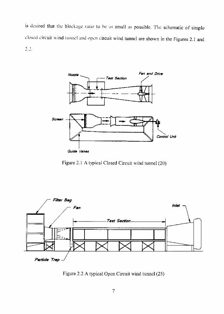
is desired that the blockage ratio to be as small as possible. The schematic of simple
closed circuit w ind tunnel and open circuit wind tunnel are shown in the Figures 2.1 and
" ) • )
Nozzle Fan »nd Drive
Screen
Guide Vanes
Control Unit
Figure 2.1 A typical Closed Circuit wind tunnel (20)
FiJter Bag
Fan
-Test Section-
Inlet
M M M M Partide Trap
Figure 2.2 A typical Open Circuit wind turmel (25)
2.1.2 Wind Tunnel Blockage Corrections
Since the w ind tunnel test section is of a confined volume, the aerodynamic
measurements obtained from the wind tunnel tests, do not resemble to that of those
obtained in infinitely spaced boundaries, such as the case of a vehicle moving on a plane
road. Various techniques are used to study the actual airflow around the geometry, and
compare it with theoretical results, which must also take into account the Reynolds
number and Mach number tor the regime of operation (1). One ofthe most important
factors to be taken care of is the boundary corrections at the walls. It is important to have
corrections for the boimdary effects, if the wind tunnel is to provide a more accurate
measure of on-road situation, where, there is no constraint to the flow above or along the
sides ofthe vehicle (3).
Limitation may not be posed on the utility ofthe wind tunnel as a developmental
tool because ofthe lack of a standard boundary correction procedure. It is because; the
differences measured between configurations that are used to guide design, are usually
insensiti\'e to boundary interference. But, a proven correction method should lead to an
improvement in the absolute accuracy of wind tunnel measurements (3). Moreover, the
fuel consumption of a vehicle depends on the drag, to some extent, and the accuracy in
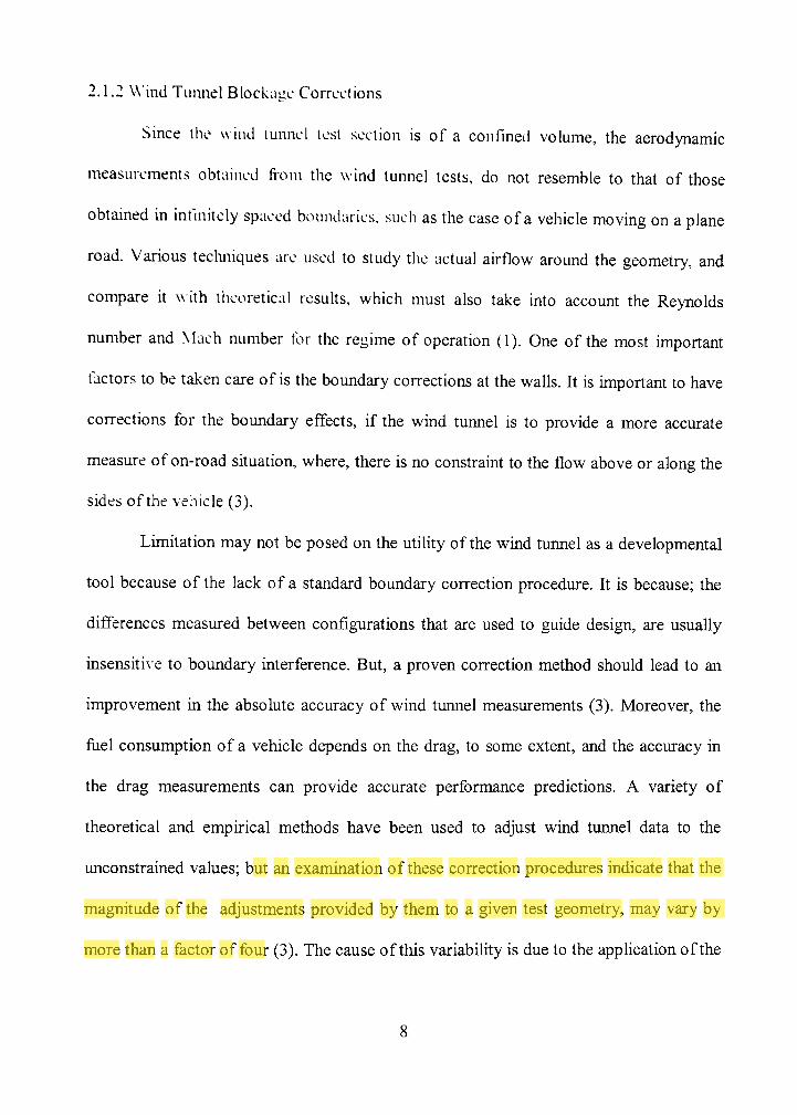
the drag measurements can provide accurate performance predictions. A variety of
theoretical and empirical methods have been used to adjust wind tunnel data to the
unconstrained values; but an examination of these correction procedures indicate that the
magnitude of the adjustments provided by them to a given test geometry, may vary by
more than a factor of four (3). The cause of this variability is due to the application ofthe
conections cun-entiv' used for aulomotives, ranging from those based on streamlined
aeronautical configurations, to those developed for geometries that have significant
regions of tlovv separation.
2.1.3 Basic Mechanism associated with Blockage Effects
The effect of the blockage can be categorized into three components. Solid
blockage, and wake blockage which cause flow speed to increase near the body
(blockage), and boundary induced wake related increment in wind axis drag. Sohd
blockage is the blockage, which is the characteristic ofthe blockage volume and the wake
bubble created next to it. The flow speed in this region of the wind tunnel test section
increases relativ ely with respect to the free stream velocity. The pressure decreases with
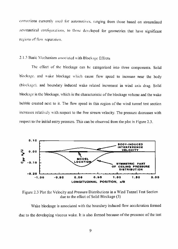
respect to the initial entry pressure. This can be observed from the plot in Figure 2.3.
0 . 1 0
^ 0 . 0 0
O - 0 . 1 0
0 . 2 0 1 1 1 ! ' JL.
BODY-INDUCED IMTERFERENCE
VELOCITY
SYMMETRIC PART OF CEIUNQ PRESSURE
DISTRIBUTION - A H W i A - ^ B h H J- ^^•^^^^^^
- 1 . 0 0 - 0 . 5 0 0 . 0 0 O.SO 1 . 0 0 LONGITUDINAL POSITION, x/B
1 . 5 0 2 . 0 0
Figure 2.3 Plot for Velocity and Pressure Distributions in a Wind Timnel Test Section
due to the effect of SoUd Blockage (3)
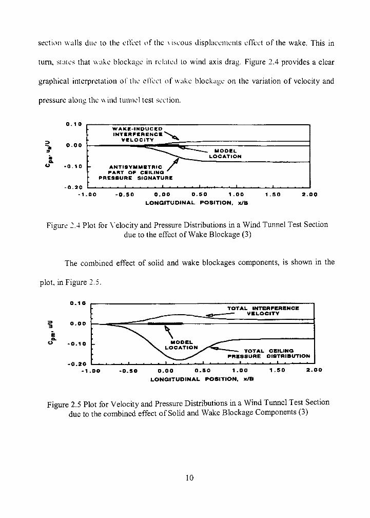
Wake blockage is associated with the boundary induced flow acceleration formed
due to the developing viscous wake. It is also formed because ofthe presence ofthe test
section walls due to the effect ofthe viscous displacements effect ofthe wake. This in
tiun, states that w ake blockage in related to wind axis drag. Figure 2.4 provides a clear
graphical inteipretation ofthe effect of wake blockage on the variation of velocity and
pressure along the w ind tunnel test section.
0 . 1 0
0 . 0 0
• 0 . 1 0
- 0 . 2 0
WAKE-INDUCED INTERFERENCE
VELOCITY
ANTISYMMBTR PART OF CEILING
PRESSURE SIGNATURE
MODEL LOCATION
' 1 . 0 0 - 0 . 5 0 0 . 0 0 0 . 5 0 1 . 0 0
LONGITUDINAL POSITION, x/B 1 . 5 0 2 . 0 0
Figure 2.4 Plot for X'elocity and Pressure Distributions in a Wind Turmel Test Section due to the effect of Wake Blockage (3)
The combined effect of solid and wake blockages components, is shown in the
plot, in Figure 2.5.
0 . 1 0
0 . 0 0
- 0 . 1 0
- 0 . 2 0
TOTAL INTERFERENCE VELOCITY
TOTAL CEILING PRESSURE DISTRIBUTION
• 1 . 0 0 - 0 . 5 0 O.OO O.BO 1 . 0 0
LONGITUDINAL POSIT ION. x/B
1 . 5 0 2 . 0 0
Figure 2.5 Plot for Velocity and Pressure Distributions in a Wind Tunnel Test Section due to the combined effect of Solid and Wake Blockage Components (3)
10
The pressure gradient produced due to the wake source that acts on the model
volume, is the reason for the wake-induced drag increment. It has been found that the
wake-induced drag increment is proportional to the square ofthe viscous drag coefficient
and independent of pressure gradient or the volume ofthe model.
2.1.4 Role of CFD in Wind Tunnel Blockage Corrections
WTien Computational methods were applied, the testing process became easier
and faster. CFD, a flow analysis tool, allowed the usage of larger models in a wind
tunnel, which reduced experimental error and problems associated with scaling (16). The
drawbacks, such as loss of coefficient of free jet and the unimpeded sound radiation were
completely eliminated. Wind tunnel testing had been a very tedious process. The
aerodynamic measurements obtained in a wind tunnel were appropriate only to that
particular wind timnel. The test results differed from the results of some other wind
timnel for the same bluff body. If the obstmction had been more appreciable in one turmel
compared to the other and in such cases, the data was not comparable.
Earher, Computational Fluid Dynamics (CFD) methods were used to simulate for
conditions under free stream. This was the easiest way for analyzing air flow around
bodies numerically. But these computational resufts, now, are generally used to compare
the experimental data, which may be biased by wall temperature. Either of the results,
computational, as well as the experimental, needs to be corrected. Though this involves
additional cost and time, the comparison of the results could lead to a more accurate
analysis ofthe flow of air over various blockages in a wind turmel.
11

Numerical modeling has so far been done by adopting many techniques, and in
combination of many types of software which involve solid modeling, grid generation,
solving, and post-processing the results. Though the computational results cannot
completely replace the experimental results, attempts have been made by many
researchers to attain accuracy to maximum extent. For this, experimentations have been
carried out on simple w ind tunnel blockages, and varying wall interference conditions.
Manv researchers have successfully generated computer codes for increasing
computational efficiency, reducing computational cost and time, and maintaining stability
of the computational techniques used. A huge content of documented works has been
provided, out of which relevant information will be discussed in the literature review.
2.2 Literature Review
Till now, significant work has been done, to have a better understanding about the
blockage corrections apphed to wind tunnels. Research has been done to determine
blockage correction equations both experimentally and computationally. This section
provides a brief review of some contributions done in this research field, so far.
2.2.1 Review of Work on Experimental determination of Blockage Correction Equation
Maskell (6), in his experiments, derived correction equations applied to flat plates
stalled at the test section centers. His theory is based on the principle of momentum
balance. His procedure did not take into account, the sohd blockage effects; but only
those effects caused due to flow separation. However, the base pressure was not known
12
under zero-blockage, and was assumed to be uniform. The blockage correction, he
proposed for bluff bodies, might be looked up al as a velocity increment. It was because,
there would be no drag increment present, as a flat plate has no volume. Maskell's
correction is based on the assumption that,
c^ = ; (2-1)
The blockage equation dev eloped by Makell to determine the blockage correction
for thin plates is.
W = j : ^ = l + (K^o^- (2.2) Cn„ A...
Thom (6), has provided the estimation of blockage correction for streamlined and
attached-flow bodies in closed-test-section wind turmels of various cross-sectional
shapes. While, Herriot (8) conducted the same experimentation to cover a range of
aeronautical body and wing shapes, and provided with tabulation of the appropriate
constants. Thom and Herriot suggested that an addictive wake-induced incremental drag
adjustment was to be appUed before the dynamic pressure correction (3).
Ramamurthy and Ng (9), have conducted wind tunnel experiments with an object
placed in series, and found that the drag was same as that obtained for a single object at
identical blockage levels. In their experiments, Ramamurthy and Ng have proposed
blockage correction equations for two-dimensional rectangular and triangular prisms for
different blockage ratios. This has facilitated the evaluation of interference effects of a
number of objects placed in series, just with experiments conducted on a single object.
Ranga Raju and Vijaya Singh (5), based on the works done by Maskell (6), Ramamurthy
13
and Ng (9) from the experiments that they conducted, found that the base pressure was
independent ofplate height, plate thickness, and the Reynolds Number, if it is greater that
10"\ But, it vai'ied with varying blockage ratios. They proposed blockage correction
equation for objects submerged in boundary layer.
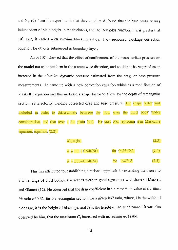
.\vvbi (10), showed that the elTect of confinement ofthe mean surface pressure on
the model not to be uniform in the stream wise direction, and could not be regarded as an
increase in the ctTective dynamic pressure estimated from the drag, or base pressure
measurements. He came up w ith a new correction equation which is a modification of
Maskell's equation and this included a shape factor to allow for the depth of rectangular
section, satisfactorily yielding corrected drag and base pressure. The shape factor was
included in order to differentiate between the flow over the bluff body under
consideration, and that over a flat plate (11). He used KD, replacing (pin Maskell's
equation, equation (2.2).
K^=<PA. (2.3)
A = 1.11 + 0.94(1/h). for 0<l/h<0.5 (2.4)
A = l.ll-0.14(//;?). for \<l/h<5 (2.5)
This has attributed to, establishing a rational approach for extending the theory to
a wide range of bluff bodies. His results were in good agreement with those of Maskell
and Glauert (12). He observed that the drag coefficient had a maximum value at a critical
l/h ratio of 0.62, for the rectangular section, for a given h/H ratio, where, / is the width of
blockage, h is the height of blockage, and H is the height ofthe wind tunnel. It was also
observed by him, that the maximum Q increased with increasing h/H ratio.
14
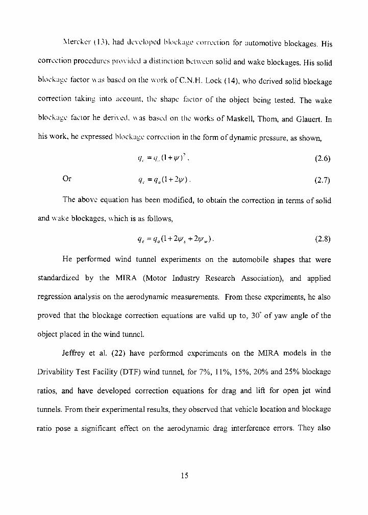
Mercker (13), had developed blockage correction for automotive blockages. His
correction procedures prov ided a distinction between solid and wake blockages. His solid
blockage factor was based on the work of C.N.H. Lock (14), who derived solid blockage
correction taking into account, the shape factor of the object being tested. The wake
blockage factor he derived, was based on the works of Maskell, Thom, and Glauert. In
his work, he expressed blockage correction in the form of dynamic pressure, as shown,
q^.=q„(\ + il/)\ (2.6)
Or q,=q,(\ + 2ii/). (2.7)
The above equation has been modified, to obtain the correction in terms of soUd
and wake blockages, which is as follows,
q^=q^(l + 2iy^+2ii/J. (2.8)
He performed wind tunnel experiments on the automobile shapes that were
standardized by the MIRA (Motor Industry Research Association), and apphed
regression analysis on the aerodynamic measurements. From these experiments, he also
proved that the blockage correction equations are vahd up to, 30° of yaw angle of the
object placed in the wind tunnel.
Jeffrey et al. (22) have performed experiments on the MIRA models in the
Drivability Test Facility (DTF) wind tunnel, for 7%, 11%, 15%, 20% and 25% blockage
ratios, and have developed correction equations for drag and lift for open jet wind
tunnels. From their experimental results, they observed that vehicle location and blockage
ratio pose a significant effect on the aerodynamic drag interference errors. They also
15
predicted that the interference error in lift measurements, increased with increase in the
vehicle size.
2.2.2 Rev icw of Work on Computational determination of Blockage Correction Equation
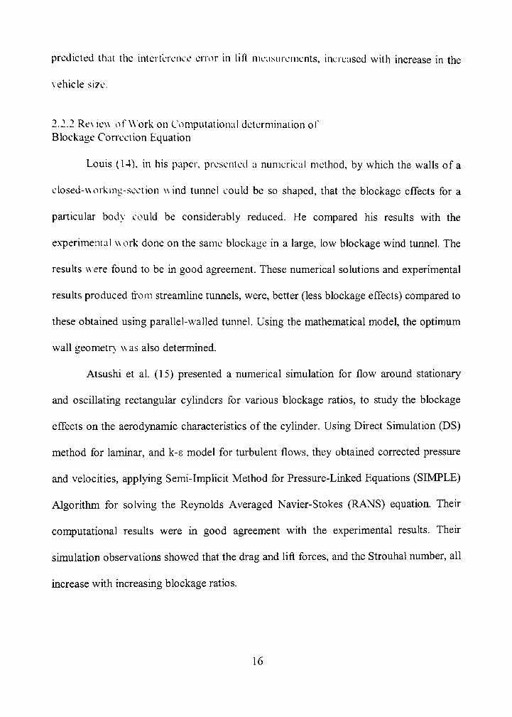
Louis (14), in his paper, presented a numerical method, by which the walls of a
closed-working-section wind tunnel could be so shaped, that the blockage effects for a
particular body could be considerably reduced. He compared his results with the
experimental work done on the same blockage in a large, low blockage wind turmel. The
results w ere found to be in good agreement. These numerical solutions and experimental
results produced from streamline turmels, were, better (less blockage effects) compared to
these obtained using parallel-walled tunnel. Using the mathematical model, the optimum
wall geometry w as also determined.
Atsushi et al. (15) presented a numerical simulation for flow around stationary
and oscillating rectangular cylinders for various blockage ratios, to study the blockage
effects on the aerodynamic characteristics of the cylinder. Using Direct Simulation (DS)
method for laminar, and k-s model for turbulent flows, they obtained corrected pressure
and velocities, applying Semi-ImpUcit Method for Pressure-Linked Equations (SIMPLE)
Algorithm for solving the Reynolds Averaged Navier-Stokes (RANS) equation. Then-
computational results were in good agreement with the experimental results. Their
simulation observations showed that the drag and lift forces, and the Strouhal number, all
increase with increasing blockage ratios.
16
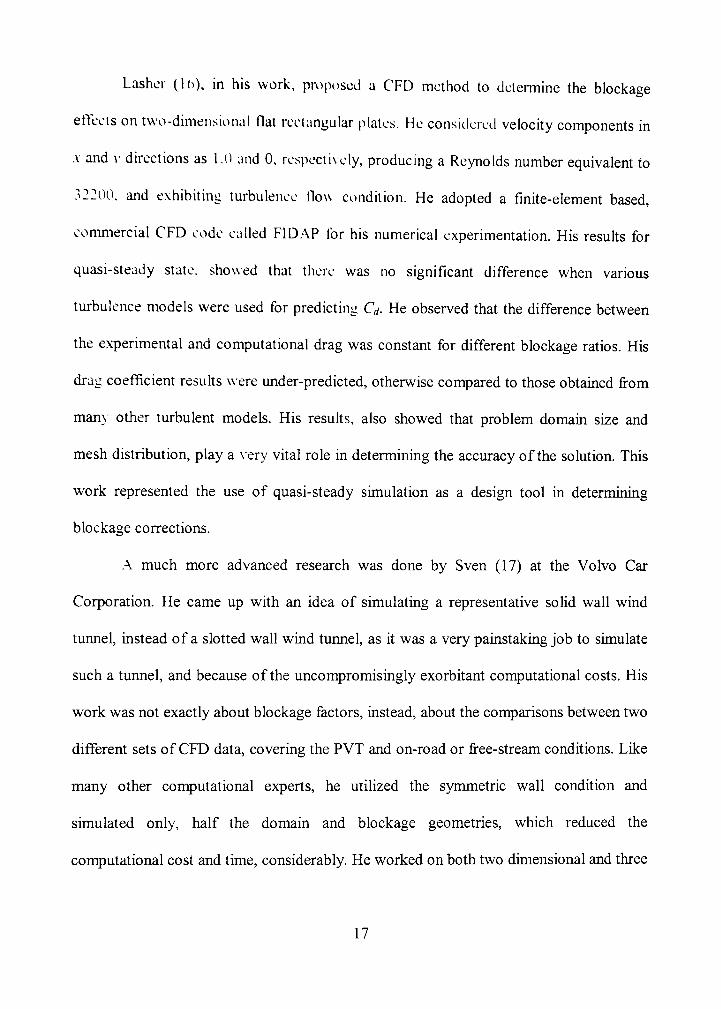
Lasher (l()), in his work, proposed a CFD method to determine the blockage
effects on two-dimensional flat rectangular plates. He considered velocity components in
.V and V directions as 1.0 and 0. respectively, producing a Reynolds number equivalent to
32200, and exhibiting turbulence flow condition. He adopted a finite-element based,
commercial CFD code called FID.XP for his numerical experimentation. His results for
quasi-steady state, showed that there was no significant difference when various
turbulence models were used for predicting C^. He observed that the difference between
the experimental and computational drag was constant for different blockage ratios. His
drag coefficient results were under-predicted, otherwise compared to those obtained from
many other turbulent models. His results, also showed that problem domain size and
mesh distribution, play a very vital role in determining the accuracy ofthe solution. This
work represented the use of quasi-steady simulation as a design tool in determining
blockage corrections.
A much more advanced research was done by Sven (17) at the Volvo Car
Corporation. He came up with an idea of simulating a representative solid wall wind
tunnel, instead of a slotted wall wind tunnel, as it was a very painstaking job to simulate
such a turmel, and because ofthe uncompromisingly exorbitant computational costs. His
work was not exactly about blockage factors, instead, about the comparisons between two
different sets of CFD data, covering the PVT and on-road or free-stream conditions. Like
many other computational experts, he utilized the symmetric wall condition and
simulated only, half the domain and blockage geometries, which reduced the
computational cost and time, considerably. He worked on both two dimensional and three
17
dimensional simulations. His tw o dimensional analysis was done as a parametric study of
wind tunnel blockage against various blockage geometric variables. Using blending
technique, like the weighting coordinates in every point, he made it possible, to test
numerous amounts of configurations w ith less meshing effort. The equation he used is,
X = a X ^^-oc) X • (2.9) nivi mcs/i nwsh I nwsh 2
For his three dimensional simulation, he used a research geometry, called Volvo
Research .-Xerodyiiamic Knowledge (VRAK) car body, second-order discretization
scheme called .X1.A.RS, standard k-s turbulence model, wall functions, and StarCD solver.
His results showed that, in case of two dimensional simulations, none ofthe parameters
tested, were significant for low blockage ratios; i.e., for blockage ratios less than 5%).
However, drag improvements are possible only at low blockage ratios. On the other hand,
the results from the three dimensional simulations, indicated a variation in wake stmcture
for X'olvo wind tunnel and free-stream conditions. Finally, he inferred that, "what's
working for one geometry may not work for another" (17).
One of the most recent works on CFD study on blockage corrections in wind
tunnels was done by Yen et al. (18). They have modeled different blockage effects in a
Climatic Wind Tunnel (CXVT) using four basic vehicle shapes, a sedan, SUV, pickup
tmck, and a minivan. Their approach was to take into account, two different nozzle-cross-
sectional areas, which differed due to the change in the nozzle height. For all the flow
simulations, they used Star-CD v.3150, a commercial CFD package from Computational
Dynamics, Inc. The flow solution domain was discretized by creating a hexahedral mesh
using ICEMCFD Engineering, Hexa software. The simulation matrix was solved using
18
the same M.XRS scheme and Suga nonlinear turbulence model. They considered domain
sizes on the CFD models varying from, 0.7*lO'' cells for an on-road simulation to,
3.4*10^ cells tor a CWT simulation. In the case of on-road situation, blockage ratio of 2%)
was considered, in order to reduce false (numerical) blockage effects. For determining the
velocitv corrections, they used the simulated Rout's (19) experimental method of
correlating the vehicle frontal velocity profiles, of a test data gathered from on-road
situation and CWT simulation. This approach resulted in a specific velocity correction
method for tests done in CWT. From this unified correlation and by applying linear
regression, \'en et al, obtained blockage factor of the form,
^.,.™„..w.wn = 0.9412C, ^JD^, + 0.9129. (2.10)
Regarding blockage corrections by vehicle upper surface centerline pressure
traces, they used a method described by Hucho (20). Hucho determined experimentally,
blockage correction factor by plotting surface static pressure coefficient measurements
from wind tunnel test, against those obtained from road tests. Applying boundary layer
theory, they corrected the surface pressure trace to an effective velocity trace, along the
vehicle surface. This was obtained by using the expression for edge surface velocity
magnitude.
f = V^^^- (2.11) o
From the results obtained from the linear regression ofthe surface pressure traces,
for both test cases, they obtained the blockage correction factor,
11/ .^ ^ =0.6740C,^[A~/D^.+0.9623. (2.12) Y V, Surface?ressure ^-^ ' ^^cl^.J / wis
19
Hence, their studv had revealed a different blockage effect in the flow field of an
automobile vary with vehicle body contour, geometry blockage ratios, and the blockage
position from the nozzle exit point (NEP).
.\t General Motors Coiporation, X'ang et al. (21), in their work, stated that the
variation ofthe blockage ctTect is attributed to the change in wind tunnel height. They
found that, due to smaller w ind tunnel heights, the blockage increased for some vehicle
models and there by increased drag. As found from their CFD study, the sum of the
corrections and the residual was not, in all cases, equal to the difference in drag
coefficient due to roimd-of errors. By changing the cross-sectional area of the virtual
wind turmel (CFD simulation), the pressure gradient effects for a given experimental
v\ ind tunnel w ere captured by CFD analysis.
AC, (Expt) = AC,(CFD). (2.13)
C,=C,(Expt)-AC,(CFD). (2.14)
20
CHAP IER3
COMPUTATIONAL METHODOLOGY
The main focus of this study is, to determine the blockage corrections for different
blockages placed in the w ind tunnel test section, using CTD methods and schemes. This
chapter mainly concentrated on the methodology followed in achieving the final goal of
this thesis. .\ detailed review ofthe various assumptions, tools, and methods used in this
research w ork, is giv en in this chapter.
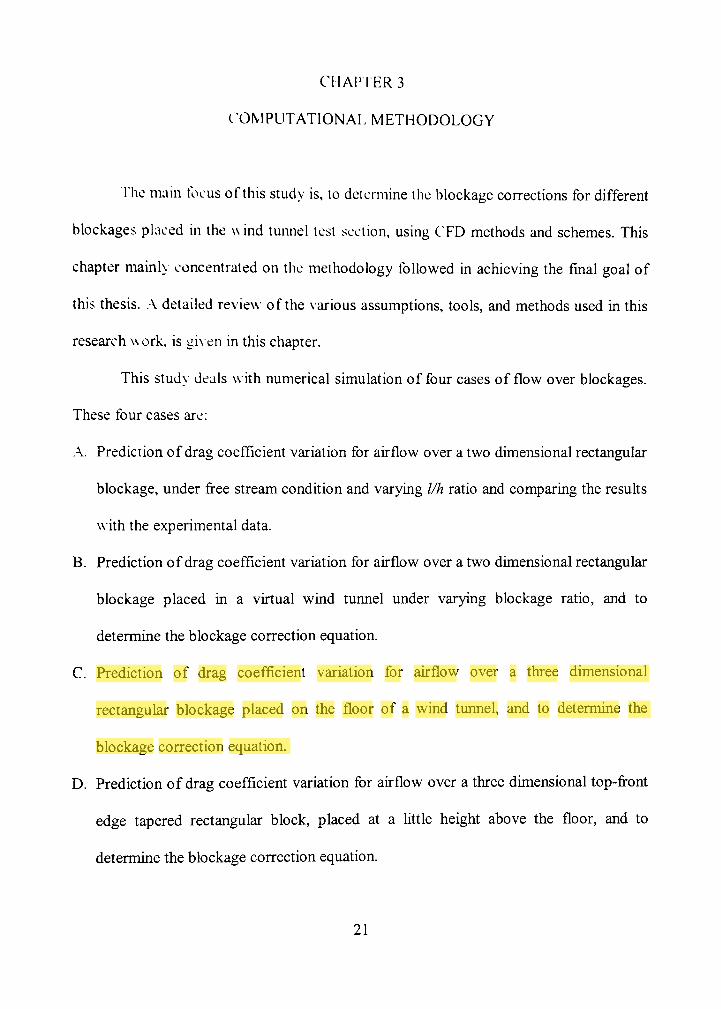
This study deals with numerical simulation of four cases of flow over blockages.
These four cases are:
.\. Prediction of drag coefficient variation for airflow over a two dimensional rectangular
blockage, under free stream condition and varying l/h ratio and comparing the results
w ith the experimental data.
B. Prediction of drag coefficient variation for airflow over a two dimensional rectangular
blockage placed in a virtual wind tunnel under varying blockage ratio, and to
determine the blockage correction equation.
C. Prediction of drag coefficient variation for airflow over a three dimensional
rectangular blockage placed on the floor of a wind turmel, and to determine the
blockage correction equation.
D. Prediction of drag coefficient variation for airflow over a three dimensional top-front
edge tapered rectangular block, placed at a little height above the floor, and to
determine the blockage correction equation.
21
3.1 .XssLiniptigns
WTiile following the methodology, many assumptions have been taken into
account. These assumptions that are considered for running the numerical simulations are
that, in the flow analysis, temperature variations and heat transfer are neglected.
Compressibility etTccts are not accounted for. Blockages are tested only at zero angle of
attack. The efTects of gravity are not considered. Flow over blockages under steady state
only, is taken into consideration. .A, uniform profile Inlet airflow velocity of Im/sec is
assumed in all the cases, irrespectixe of the variation of the Reynolds number. While
determining the drag coefficient, the effect of only the pressure drag is considered.
3.2 Computational Setup and Solution Procedure
The details ofthe test section dimensions, blockage dimensions and their location
in the testing domain are discussed. The modeling of the test section domains and the
blockages, is done using Pro/E Wildfire ofthe PTC Inc. The modeling is done taking into
account, all the dimensions in millimeters.
3.2.1 Domain Layout Considerations
In order to reduce the difficulties in the analysis two dimensional flow cases, three
dimensional models are created, in which the third dimension, which is the projected
thickness of the two dimensional sketch, has no effect on the two dimensional flow
analysis for drag, according to Ramamurthy and Ng (9). The blockages used in the wind
22
tunnel test section are rectangular, in case of two dimensional testing. The blockage ratio
in the two dimensional case is defined as the ratio ofthe height ofthe blockage to the
height ofthe test section or the domain.
H (3.1)
For the free stream flow condition, \% blockage ratio is considered so that, the
efTect ofthe walls on the flow over the blockage is very negligible. The dimensions ofthe
computational setup are provided in detail, in the Figures 3.1 and 3.2.
Velocity. V=1000mm/sec Free Streem Domain
H=99h
Figure 3.1 Layout ofthe free stream domain with blockage; height ofthe blockage, h=400mm
In the above case, the l/h ratio is varied and hence the length of the blockage
changes with it. The following table, Table 3.1, illustrates the variation.
23
able 3.1 Magnitude of I for different l/h ratios
l/h Ratio
/ in mm
0,7
280
1,2
480
2.0
800
25
1000
3.0
1200
6.0
2400
Ve/odty. V=I000mmyse€ Wind Tunnel Test Section
H
Figure 3.2 Layout ofthe wind tunnel test section with the rectangular blockage, h=400mm
The rectangular blockage has constant dimensions. So, the height of the wind
tunnel is decreased with increasing blockage ratio. The blockage is seen to that, it is
always located in the midway ofthe total height ofthe test section. Table 3.2 depicts
magnitudes ofthe height ofthe test section and the vertical location ofthe blockage, with
varying blockage ratio.
Table 3.2 Height ofthe wind tunnel and the vertical location ofthe blockage for 5%), 10% and 15%) blockage ratios
Blockage Ratio %
H (x*h) m m
K (x*h) m m
5
6800 (17h)
3200 (8h)
10
3600 (9h)
1600 (4h)
15
2800 (7h)
1200 (3h)
24
The three dimensional model created, is a rectangular solid-wall wind tunnel test
section. The test section and Uie blockage dimensions have been taken with reference to
the automobile model dimensions suggested by the MIRA and experimental data
provided by the SAE in the reference (3). The blockage ratio in the three dimensional
flow analysis is defined as the ratio ofthe projected cross sectional area ofthe blockage,
to the cross sectional area ofthe w ind tunnel test section. This is denoted by the equation,
<P,D = Us I Section / o .^\
w*h
W*H
The height of the test section in the three dimensional case is also varied with,
change in the blockage ratio. So, the initial height ofthe test section and the dimensions
of the blockages are taken as standard, at 15%) blockage ratio. Then, keeping the
dimensions of the blockage constant, the height of the wind tunnel test section is
increased proportionally, for 10%) and 5% blockage ratios.
In the present research, the blockage geometries considered are rectangular
cuboid and a rectangular block with top-front edge tapered. Both the geometries are
created to have their maximum projected dimensions to be equal. The simple rectangular
blockage is positioned on the floor ofthe wind tunnel test section. XVhereas, the blockage
with top front edge tapered, is positioned at a certain height above the floor. In both the
cased, the positions ofthe blockages with respect to the floor are unaltered, irrespective
of the changes in the test section height. The actual layout of the blockages and their
location in the wind tunnel test section, are as shown in the Figure 3.3 and 3.4.
25
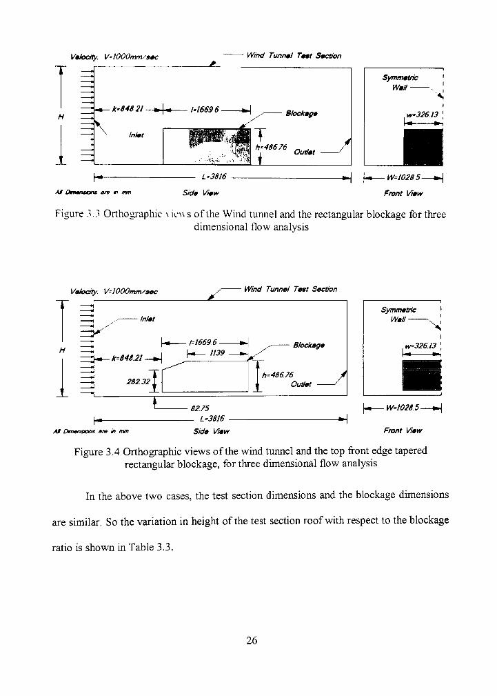
V'eJodty. V^JOOOmm^sec Wind Tunnel Teal Section
= \
1^84821 • I'1669 6- Blockage
Inlet
•y ' ^ ^
T h'48676
J Outlet J L'38l6
AM Ounansans are m mm Side View
W=I0285-
Front View
Figure 3.3 Orthographic v iew s ofthe Wind tunnel and the rectangular blockage for three dimensional flow analysis
Velodty. V=1000mmysec
H
_!_
^ Wind Tunnel Test Section
Inlet
1=16696-
. k=8482I
282.32
1139 Blockage
l \ r
I h=48676 Outlet J
Symmetric Wall-
X , w-326.13
At Dmensions are in mm
82.75 - L=3816 -
Side View H
W=1028.5
Front View
Figure 3.4 Orthographic views ofthe wind tunnel and the top front edge tapered rectangular blockage, for three dimensional flow analysis
In the above two cases, the test section dimensions and the blockage dimensions
are similar. So the variation in height ofthe test section roof with respect to the blockage
ratio is shown in Table 3.3.
26
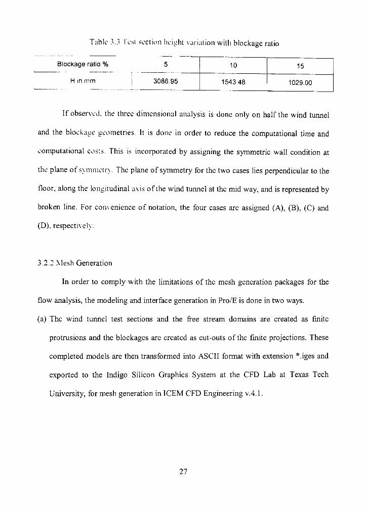
Table 3.3 lest section height variation with blockage ratio
Blockage ratio %
H in mm
5
3086.95
10
1543.48
15
1029.00
If observed, the three dimensional analysis is done only on half the wind tunnel
and the blockage geometries. It is done in order to reduce the computational time and
computational costs. This is incoiporated by assigning the symmetric wall condition at
the plane of synimetrv. The plane of symmetry for the two cases hes perpendicular to the
floor, along the longitudinal axis ofthe wind turmel at the mid way, and is represented by
broken line. For convenience of notation, the four cases are assigned (A), (B), (C) and
(D), respectively.
3,2,2 Mesh Generation
In order to comply with the hmitations of the mesh generation packages for the
flow analysis, the modeling and interface generation in Pro/E is done in two ways.
(a) The wind tunnel test sections and the free stream domains are created as finite
protmsions and the blockages are created as cut-outs ofthe fmite projections. These
completed models are then transformed into ASCII format with extension *.iges and
exported to the Indigo Silicon Graphics System at the CFD Lab at Texas Tech
University, for mesh generation in ICEM CFD Engineering v.4.1.
27
(b) The blockages are created as finite protrusions and then transformed into ASCII
format with extension *.stl and exported to PHOENICS v.3.5 flow analysis software
for mesh generation.
The ICIAI Cf'D Engineering package is exclusive mesh generation software
developed bv .\NSYS. Inc. It is a meshing tool developed for CFD purposes, as CFD
apphcations require computational domain for analysis. ICEM CFD possesses the ability
to generate a wide variety of mesh elements. In the present work, the mesh generation is
done with hexahedral grid using ICEM CFD Hexa tool. This package also facilitates
assigning of the boundary conditions to the walls of the computational domain and the
blockage.
PHOENICS is flow analysis software developed by CHAM Ltd. The domain
creation, mesh generation, assignment of the boundary conditions, flow model, solver
end time and the number of iterations, is done in the pre-processor called VR Editor. Due
to the limitations ofthe package, symmetric wall conditions were not apphed for analysis
done in PHOENICS. So, the analysis had to be done on the whole model in cases (C) and
(D). For cases (A) and (B), the thickness ofthe domain has been taken as lOh in order to
comply with the symmetric wall condition.
The mesh is generated with uniform cell spacing at the vicinity ofthe blockage.
But, a geometrically increasing cell size is considered, as the cell position moves away
from the blockage. This also saves computational time and cost. The mesh generated
using ICEM CFD for the four cases, taking a single blockage of each case, are shown in
the Figures 3.5, 3.6, 3.7 and 3.8. The mesh generated using the VR Editor in PHOENICS,
28
are shown in Figures 3.9, 3.10, 3.11 and 3.12. The mesh has been generated for various
blockages using Blending Technique, by which the mesh sizes of intermediate blockages
are determined using the equation (2.9). This method helps achieve a smooth transition of
the mesh sizes for test domains from lower blockage ratios to higher and vice versa. In
order for the blending technique to be implemented, the mesh sizes ofthe two blockage
ratios are to be known. The blending factor for the case (A) are taken as, 0.8, 0.4, 0.2 and
0.1. Taking the meshl and mesh2 as the first and last mesh sizes, the intermediate mesh
sizes are determined using the above blending factors, respectively. For the remaining
cases, the blending factor is taken as 0.8.
29
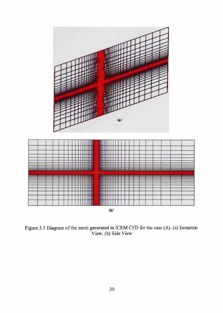
Figure 3.5 Diagram ofthe mesh generated in ICEM CFD for the case (A), (a) Isometric View, (b) Side View
30
• • • • • ^ H ^^M ^^H ^^^H ^•IH ^^^^B
^^^H i^^^l ^^H ^^1 ^ •
^ ^ i ^ B i ^ ^^•••••H
^ _
^^^ ^ ^ H
^H • 1
B •
= ^
^^s ^^B ^^1 • i • B •
H
==
^^ ^ H HI • • • •
III llllll
llllllll
^s ^H ^1 • • • I 1
H • • • • H B III
I • 1 • • s
llllllllllllll
HI Ml 1 1 1 I • • a III
llllllllllllll
II
1 iii
iiiiii
iii
1 m
ill
1 IIIIIIIIIIII
ill IIIII IIIII IIIII lilll IIIII mil • • • 1 1 •iiii :::!!
lllllil llllllll IIIII IIIII IIIII llllll mill llllll llllll
!!!:!!
llllllll lllllli llllllll llllllll llllllll II II II l l l l l l i
1II II n i l II
11 i l l : II
lllllli llllll llllll llllllll llllllll llllllll llllllll
llllllll
II llllll lllllli
IIIIIIIIIIII IIIIIIIIIIII lllllllll IIII lllllllll IIII lllllllll l i i i
II III!
lllllllll:;;!:
• nil
1 1 ll
llllllllllll
lltt
lllllllllll
IIII II II l l l l l l l l l l l l l l l l l l l l • I I I I I II l l l l l l l l l l l l l l l l l l l l I I I I I ! II IIII 1 II II II I I I I
IIIII 1 IIIII
l l l l l l i IIIII IIIII IIIII IIIII
III II II
• • • llllllll 1 • • • llllllll 1 • • •
I I I II l l l l l l i III 1 1 IIIII II 1 1 III 1 I I I 1 I II
1 1 1 1 II II
11 II II 1 1 1
III
llllll
llllll
lll
llllllll
lllllll
llllllll
lllllll
• • 1 I 1 1 1 1
llllllll
lllllll III
lllll
llllllllll
• ^m
III
=
I • • • nn • • - •
III
^
^s ^ B ^ 1
• B • • •
• • • • m I^H
• —
III
^
— ^M ^ H
• B • • •
• • • • • ^^m
IIII
^ s
^^ ^ H ^M • B • •
• • • • i ^
^ ^ 1 ^H ^H • III •
• ^ ^g • • ^ ^ H
^m ^^^ ^ ^ ^=
^ = ^ ^ H ^ ^ H ^ H ^H ^M n •
• • ^ ^ ^ ^ 1 imm • • • i ^^^im
^ —
=
^^^H ^ ^ ^ 1
^•1 ^ H ^M ^M •
• • ^ • i ^^B ^^^g ^ ^ ^ H
^ • • H l
• i ^ ^ ^^^H • ^ 1 ^^1 ^H ^H •
• •i ^
HHH ^^Hl ^^^^g ^^^^m
^^^^m\ • M ^ ^
^ 1 •i^i ^ H B •
(tj
Figure 3.6 Diagram ofthe Mesh generated in ICEM CFD for the case (B). (a) Isometric View, (b) Side View
31
(b)
Figure 3.7 Diagram ofthe mesh generated in ICEM CFD for the case (C). (a) Isometric View, (b) Side View
32
(b)
Figure 3.8 Diagram ofthe mesh generated in ICEM CFD for the case (D). (a) Isometric View, (b) Side View
33
1 1 \
wmmm
\ \^ ; V 1
HIM
IIIII
llllll m
il lllil
1 III
! llllll m
il 1)11 1
Ml)
nil 1
mil
IIIII h-IM
11111111111 I I I I 111
llllllllBIH llilllllil: II III
• • • • l l l l l l i 1 III • • • l l l l l l l l 1 III
fftfft 1 t u 1 r ii
t ti
I I 1II •t 11
>i> , 1 1 ••
I I I I 1 I I I III 1 : 1 l i l l I I I ! 1 . I l l
IIII 1 n i l IIII 1 I I I IIII 1 I I I mil, m llllll:..nil!
II tt ft" ft XL
m i l l
i'lH
• • •
(a)
(b)
Figure 3.9 Diagram ofthe mesh generated in PHOENICS VR Editor, for the case (A). (a) Side View, (b) Front View
34
" =
( fe
1
E ±:: l:f:-: • I F ! T T T
II • T ,n L... : 1
_ X L_L i .ALL...
r"T"~
:::::|::::i.. _::;-iiiilB 4 " "
...|,± Ej
•
—
___ 1
t ' 1 t ' t
v^ - -T f j r
1 1
1 1 (aj
(b)
\
1 ' ' 1 i i i
I I I 1 1 1 i l l
1
' I 1 1 i
I I I I M M M M
II 1 1 1 M
1 !
i_^
I I I
1 1 1 1 1
1
I 1 1
1 1
1 1
1
1
1 ! i ! • I
' 1 ' i l l !
^'nx j__i._i_i^ < 1 1 1 : 1 1
l l l l l i l
1 , [•"
tc
111| |i 1111IIII h 11II1 |44tH - T T ' " ••'! T • I I I I 1 1 . . - - . : : • -+H—M ' ' 1 1 1 1—'—H
T r ' I 1 ' ' 1 !
:i : : : ::::
. 1 — , — } — j — ' — ' • — 1 — 1 — 1 — 1 — 1 — 1 — ?
— I l l 1 , , 1 1 i , i
- • ' • 1 1 I I I
: : : : : i z X
Figure 3.10 Diagram ofthe mesh generated in PHOENICS VR Editor, for the case (B). (a) Side View, (b) Front View
35
(a)
•IIII H
1
T
m (b)
X
Figure 3,11 Diagram ofthe mesh generated in PHOENICS VR Editor, for the case (C). (a) Side View, (b) Front View
36
(a)
:x
= mr:
(b)
Figure 3.12 Diagram ofthe mesh generated in PHOENICS VR Editor, for the case (D). (a) Side View, (b) Front View
37
The mesh si/es ofthe domains of all the four cases are tabulated in Table 3.4 and 3.5, as
follows.
Table 3.4 The mesh si/es ofthe computational domain for case (A), taking into account the blending factor a
Blending factor a
l/h
Cacc(A) ' ICEMCFD ^a-c (A) PHOENICS
Mesh sizes
0.7
45700 56280
0.8
1.2
48100 57960
0.4
2
51940 61320
0.2
2.5
54340 63000
0.1
3
55640 63840
6
56740 64680
Table 3 5 The mesh sizes ofthe computational domain for cases (B), (C) and (D), taking into account the blending factor a
Blending factor a
Blockage ratio%
Case(B)
Case (C)
Case (D)
ICEMCFD PHOENICS
ICEMCFD PHOENICS
ICEMCFD PHOENICS
5
0.8
10 15
Mesh sizes
46980 111300
81400 156000
54140 106560
37680 84820
65470 109200
41040 82510
35360 78200
61480 97500
37770 74000
38
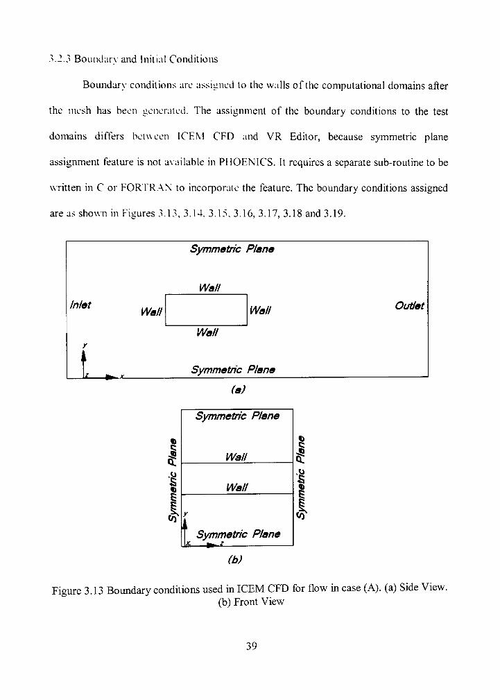
3.2.3 Boundarv and Initial Conditions
Boundary conditions are assigned to the walls ofthe computational domains after
the mesh has been generated. The assignment of the boundary conditions to the test
domains dilTers between ICEM CFD and VR Editor, because symmetric plane
assignment feature is not av ailablc in PHOENICS. It requires a separate sub-routine to be
written in C or FORTR.A,N to incorporate the feature. The boundary conditions assigned
are as shown in Figures 3.13, 3.14. 3.15, 3.16, 3.17, 3.18 and 3.19.
Symmetric Plane
Wall
Inlet Wall Wall
Wall y
1^ Symmetric Plane
(a)
Outlet
(b)
Figure 3.13 Boundary conditions used in ICEM CFD for flow in case (A), (a) Side View. (b) Front View
39
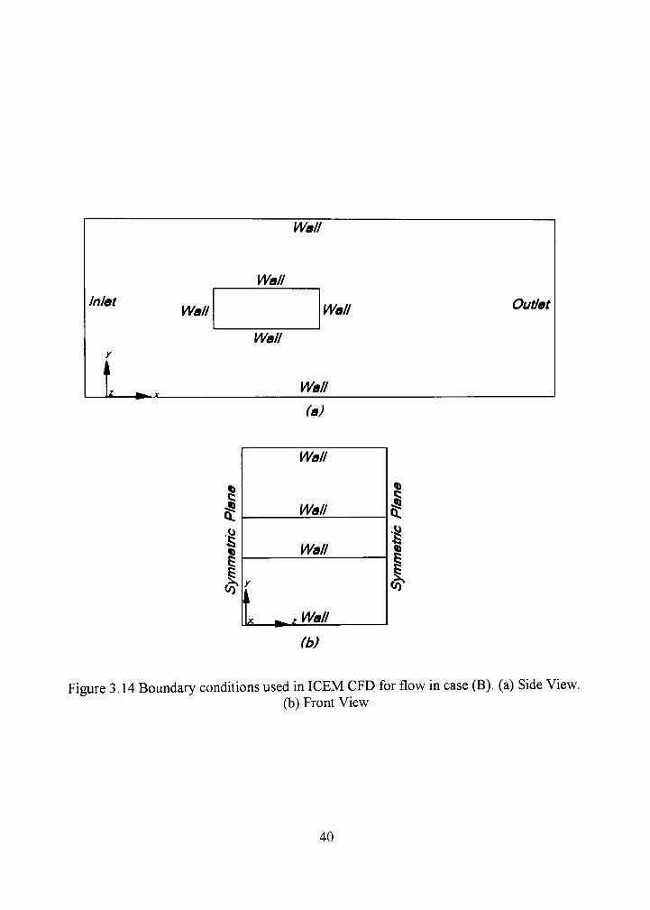
Inlet
y i I — ^ - j ^
Wall
Wall
Wall
Wall
Wall
Wall
Outlet
(a)
(b)
Figure 3.14 Boundary conditions used in ICEM CFD for flow in case (B). (a) Side View. (b) Front View
40
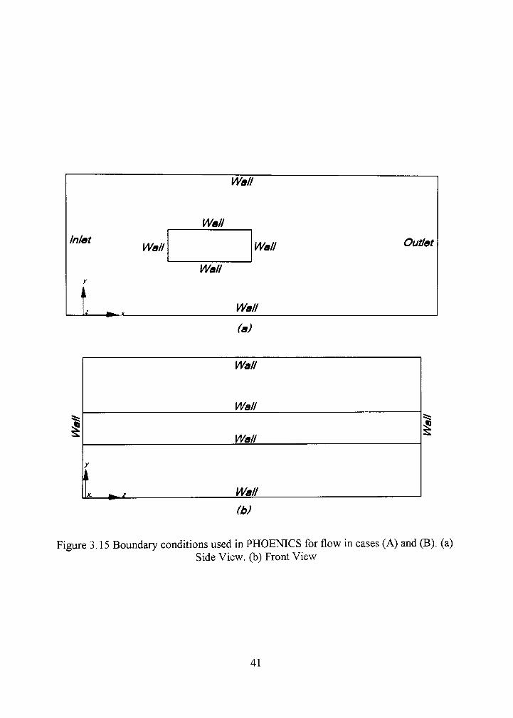
Inlet
y
l
Wall
^ r
Wall
Wall
Wall
Wall
Wall
(a)
Outlet
(b)
Figure 3.15 Boundary conditions used in PHOENICS for flow in cases (A) and (B). (a) Side View, (b) Front View
41
Inlet
y
t Wall - ^ - j c —
Wall
Wall
Wall
Wall Wall
Outlet
(a)
I
Wall
\ Wsl, """ i£ toJZ 1
1 " S
ymm
etric
Pla
ne
(b)
Figure 3.16 Boundary conditions used in ICEM CFD for flow in case (C). (a) Side View. (b) Front View
42
Inlet
V
I \ Wall Wall
Wall
Wall
Wall Wall
Outlet
(a)
Wal
l
y
i X.
Wall """ ^f 1
Wall
Wall
Wall
Wal
l
Wall
(b)
Figure 3.17 Boundary conditions used in PHOENICS for flow in case (C). (a) Side View. (b) Front View
43
Inlet
y
t — ^ - x —
Wall
Wall
Wall
Wall
Wall Wall
Wall
Outlet
(a)
Wall
i Wall
L ^ . Wall
Wall
Wall
I
I (b)
Figure 3.18 Boundary conditions used in ICEM CFD for flow in case (D). (a) Side View. (b) Front View
44
Inlet
y
i i— — ^ ^ x —
Wall
Wall
Wall
Wall
Wall Wall
Wall
Outlet
(a)
1
I ^ ^
Wall
Wall
Wall
Wall Wall
1
Wall
(b)
Figure 3.19 Boundary conditions used in PHOENICS for flow in case (D). (a) Side View. (b) Front View
45
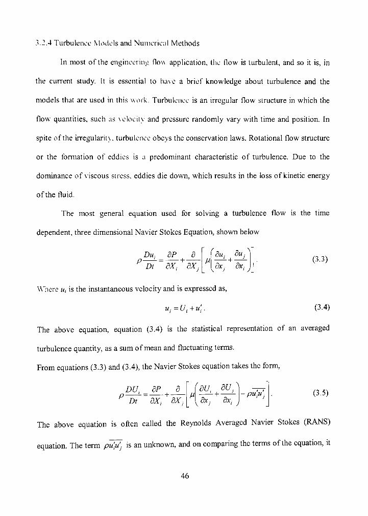
3.2.4 Turbulence Models and Numerical Methods
In most ofthe engineering flow application, the flow is turbulent, and so it is, in
the current study. It is essential to have a brief knowledge about turbulence and the
models that are used in this work. Turbulence is an irregular flow structure in which the
flow quantities, such as velocity and pressure randomly vary with time and position. In
spite ofthe irregularitv, turbulence obeys the conservation laws. Rotational flow structure
or the fomiation of eddies is a predominant characteristic of turbulence. Due to the
dominance of viscous stress, eddies die down, which results in the loss of kinetic energy
ofthe fluid.
The most general equation used for solving a turbulence flow is the time
dependent, three dimensional Navier Stokes Equation, shown below
DM,. dP d p—•- = +
Dt dX, dX,
M ''du, du.^ —'--\-—-dxj dx-
(3.3)
Where M, is the instantaneous velocity and is expressed as,
u. = U- + u'.. (3.4)
The above equation, equation (3.4) is the statistical representation of an averaged
turbulence quantity, as a sum of mean and fluctuating terms.
From equations (3.3) and (3.4), the Navier Stokes equation takes the form.
DU, dP d p - = + ^ Dt 5X. dX;
M ' + ^ 8xj dx,
•puy. (3.5)
The above equation is often called the Reynolds Averaged Navier Stokes (RANS)
equation. The term p z ^ is an unknown, and on comparing the terms ofthe equation, it
46
was found to be turbulence stresses. These stresses were later called Reynolds stresses,
named after the person w ho proposed the equation. Due to the presence ofthe stress term,
the R.\NS equation is not closed. In order to obtain a closure problem for the above
equation, several models have been proposed to express the stress in terms of dependent
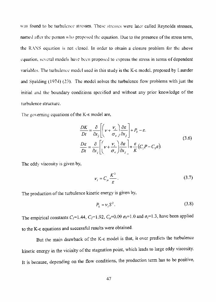
variables. The turbulence model used in this study is the K-e model, proposed by Launder
and Spalding (1974) (23). The model solves the turbulence flow problems with just the
initial and the boundary conditions specified and without any prior knowledge of the
turbulence structure.
The go\eming equations ofthe K-s model are,
DK _ d Dt dXj
Ds _ d
Dt dx,
v + -V,
V.
ds
E J dX;
ds
+ P,-s.
dx, +Uc,p-c,s).
The edd\ viscosity is given by.
^t=C^ K'
(3.6)
(3.7)
The production ofthe turbulence kinetic energy is given by,
P,=y<s\ (3.8)
The empirical constants C;=1.44, C2-1.92, Q=0.09 <TA=1.0 and a,=1.3, have been applied
to the K-s equations and successful resufts were obtained.
But the main drawback ofthe K-s model is that, it over predicts the tiirbulence
kinetic energy in the vicinity ofthe stagnation point, which leads to large eddy viscosity.
It is because, depending on the flow conditions, the production term has to be positive,
47
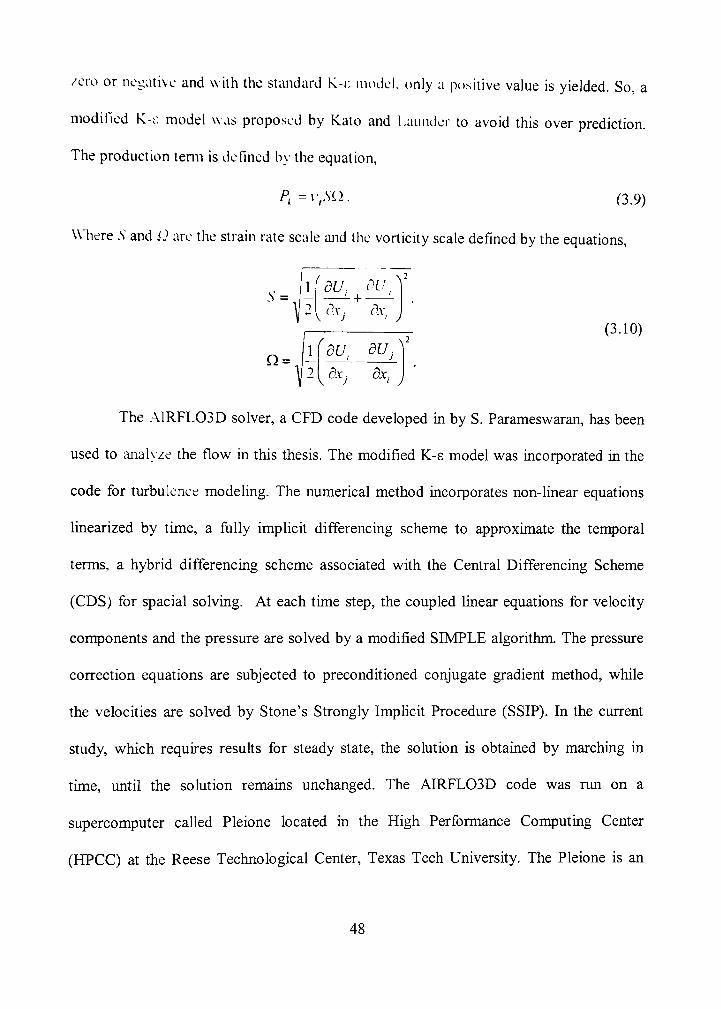
zero or negative and w ith the standard K-t; model, only a positive value is yielded. So, a
modified K-i: model was proposed by Kato and Launder to avoid this over prediction.
The production temi is defined by the equation,
^*=>V^'ii- (3.9)
Where .V and <2 are the strain rate scale and the vorticity scale defined by the equations.
V ^ • •; ^-v-
Q = j ' i
(3.10)
dU, dUj
The .\1RFL03D solver, a CFD code developed in by S. Parameswaran, has been
used to anah ze the flow in this thesis. The modified K-s model was incorporated in the
code for turbulence modeling. The numerical method incorporates non-linear equations
linearized by time, a fiilly implicit differencing scheme to approximate the temporal
terms, a hybrid differencing scheme associated with the Central Differencing Scheme
(CDS) for spacial solving. At each time step, the coupled linear equations for velocity
components and the pressure are solved by a modified SIMPLE algorithm. The pressure
correction equations are subjected to preconditioned conjugate gradient method, while
the velocities are solved by Stone's Strongly Implicit Procedure (SSIP). In the current
study, which requires results for steady state, the solution is obtained by marching in
time, until the solution remains unchanged. The AIRFL03D code was run on a
supercomputer called Pleione located in the High Performance Computing Center
(HPCC) at the Reese Technological Center, Texas Tech University. The Pleione is an
48
SGI Onvx2 system with 5()-3()() MH/ processors, and 56 GB of shared RAM. The
programming language used is the FORTRAN 90 GL.
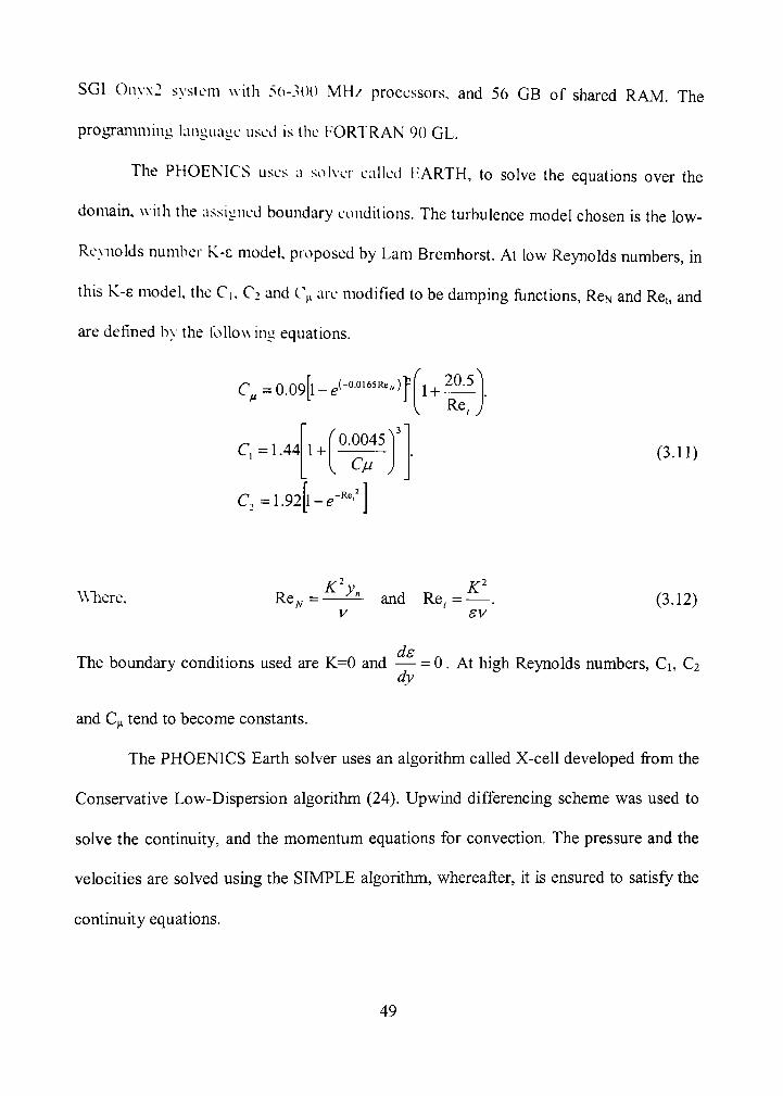
The PHOENICS uses a solver called 1;ARTH, to solve the equations over the
domain, w ith the assigned boundary conditions. The turbulence model chosen is the low-
Reviiolds number K-s model, proposed by Lam Bremhorst. At low Reynolds numbers, in
this K-E model, the Ci, C: and C\, are modified to be damping fimctions, RCN and Ret, and
are defined b\ the follow ing equations.
C^=0.09[l-e(-°°'"'' '-'f ^, 20.5^ 1 +
V Re ' J
C, =1.44 1 + ^0.0045^'
Cp
C =1.92 [ l - . - '
(3.11)
Where. Re;,= ^'y. and Re, =
ds
K'
sv (3.12)
The boundary conditions used are K=0 and — = 0. At high Reynolds numbers, Ci, C2 dy
and C^ tend to become constants.
The PHOENICS Earth solver uses an algorithm called X-cell developed from the
Conservative Low-Dispersion algorithm (24). Upwind differencing scheme was used to
solve the continuity, and the momentum equations for convection. The pressure and the
velocities are solved using the SIMPLE algorithm, whereafter, it is ensured to satisfy the
continuity equations.
49
The solutions obtained fi-om the solvers are post-processed to interpret the data
into useful graphical formats. The data is also used for calculating the drag coefficients
for the four cases. The definition for drag coefficient used in both the cases is same and is
represented bv the following equation.
Co=T^^^- (3.13)
- I M-',„"
Wliere, FD is the drag force acting on the body due to the pressure acting on the body,
produced as a result ofthe flow, and V is the velocity of air in the direction of flow. A
detailed analysis ofthe data obtained from the solvers will be present in the next chapter.
50
CHAPTER 4
RI'SULTS AND DISCUSSIONS
The computational methodologv in the chapter 3 is used to determine the flow
anah SIS for the four cases mentioned in the same chapter. The results obtained from this
computational anahsis are compared and blockage correction equations are proposed.
The computational results obtained from case (A) are compared with those in the
reference (26). Due to imavailability of the wind tunnel experimental results for cases
(B). (C) and (D), the results obtained from PHOENICS are used to provide the blockage
correction equations for the results obtained from AIRFL03D.
The data obtained from the AIRFL03D and the PHOENICS Earth solvers are
analyzed after Post-processing in ENSIGHT and GUI Post-processor in PHOENICS,
respectively. The number of iterations used for each case is 2000. A detailed description
ofthe results obtained from each test case is presented in this chapter.
The results in each case include the pressure signatures and velocity profiles
plotted along the Une passing the longitudinal dimension (i.e., the direction of flow) of
the domain and touching the upper surface ofthe blockages placed in the domain. For the
cases (C) and (D), the data sets for the plots are obtained about the longitudinal plane of
symmetry. The other plots include the drag coefficient and drag correction plots. The
following sections deal the results case by case. The pressure signature is the pressure
coefficient, which is determined by the equation (4.1).
51
S = - i ""•'• (4.1)
4.1 Case (A) Two Dimensional Flow around a rectangular section subjected to an unconstrained flow field
The computational domain, with the blockage, as shown in Figure 3.1 and the grid
structure as in Figure 3.5. indicate clearly that the computational domain is symmetric
along a horizontal line passing through the middle ofthe rectangular blockage. Since a
verticalh symmetric velocity profile (constant velocity of 1000 mm/sec) has been
applied, the flow pattern also has to be symmetric, vertically. Results have been obtained
both in PHOEMCS and AIRFL03D, only along the upper horizontal line of the
rectangular blockage, due to the symmetric flow condition, i.e., along the line AB in
Figure 4 1.
A B
Figure 4.1 Line along which the Pressure and Velocity Distributions are obtained in Two Dimensional case
52
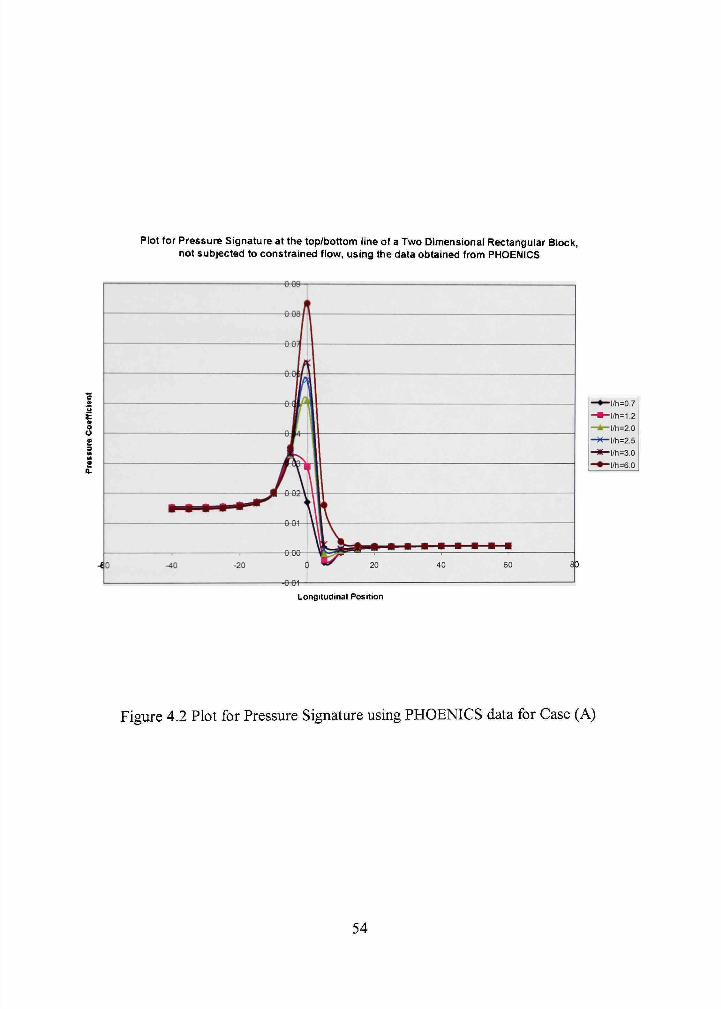
It can be observed from the pressure signature plot of Figure 4.2, that the pressure
away form the blockage is not effected. It remains almost constant over a considerable
distance from the test domain entrance. There is a sudden increase in the pressure at a
little distance in front ofthe blockage; but it decreases as it approaches the edge ofthe
blockage. Past the blockage, there is fiuther decrease in the pressure and reaches below
zero pressure. With a little increase past zero pressure, the pressure past the blockage
tends to be constant till the exit ofthe test domain.
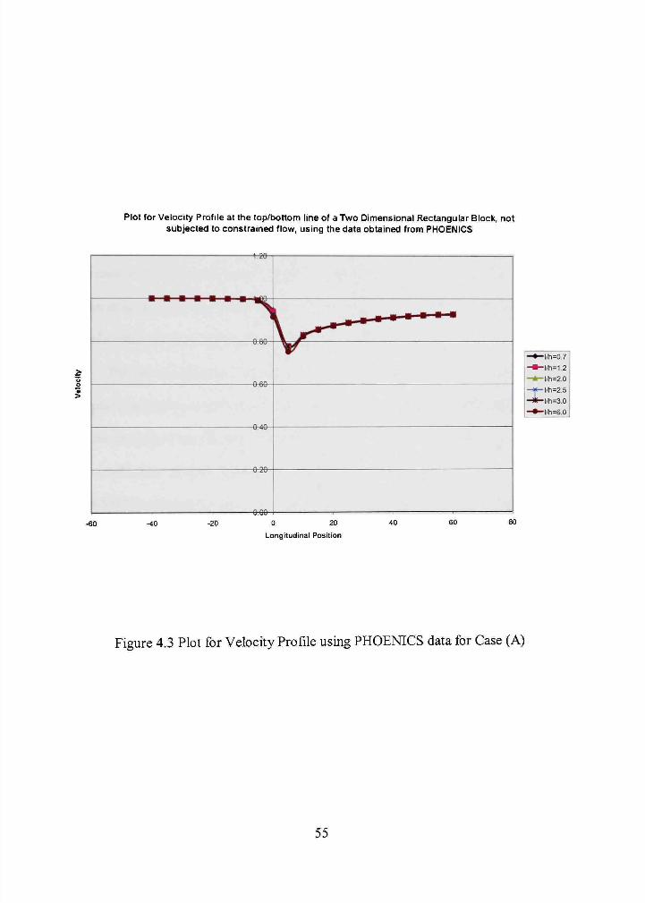
The velocity also remains constant at the entrance ofthe test domain to almost up
to the front end of the rectangular blockage. It decreases further, past the blockage and
with a shght increase, again tends to remain constant till the domain exit. It can also
foimd that the velocity profile has a very little variation with the change in the l/h ratio, in
the vicinity ofthe blockage. The variations can be clearly observed in the velocity profile
plot from Figure 4.3.
53
Plot for Pressure Signature at the top/bottom line of a Two Dimensional Rectangular Block, not subjected to constrained flow, using the data obtained from PHOENICS
-Wl=0,7
-l/h=1,2
-l/h =2,0
- I * =2.6
-l/h=3,0
-l/h=6,0
Longitudinal Position
Figure 4.2 Plot for Pressure Signature using PHOENICS data for Case (A)
54
Plot for Velocity Profile at the top/bottom line of a Two Dimensional Rectangular Block, not subjected to constrained flow, using the data obtained from PHOENICS
-6:69-
-6:46-
-6:26-
0.00
-l/h =0,7
-l/h=1,2
-|/h=2.0
-l/h=2.5
-l/h =3,0
-l/h =6,0
.60 0 20
Longitudinal Position
Figure 4.3 Plot for Velocity Profile using PHOENICS data for Case (A)
55
The sudden rise in the pressure can be attributed to the high pressure, due to
stagnation in front of the blockage and the change in the velocity direction. The
inconsiderable variation in the velocity can be atiributed to the reason that, the wall
conditions are too far from the blockage to elTect. The sudden drop in the velocity beyond
the blockage is due to the formation of wake bubble at the rear of the blockage. The
effect of wake extends till the domain exit. This might possibly be the reason for the
ditTerence in the inlet and outlet velocity magnitudes. The same reason holds for the
sudden drop and rise of pressure beyond the blockage It can also be seen that the wake
does not effect the flow much, above or below the blockage.
The plot for variation of drag coefficient with varying l/h ratio is also plotted. The
drag plot obtained from PHOENICS data shows a gradual decrease in the drag coefficient
with the increase in the l/h ratio. The variation is very little compared to the experimental
drag coefficient, plotted against l/h. AIRFL03D yields higher results compared to,
PHOENTCS and experimental data. It also shows a considerable drag variation. Figures
4.4, 4.5, and 4.6 show the drag coefficient variations for the data from the three sources.
The drag correction for the computational results can be obtained from a plot
drawn for computational drag against experimental drag. Linear regression is applied to
the data points in the plot and the linear equation obtained from it is the blockage
correction equation. The plots for the blockage correction can be seen in Figures 4.7 and
4.8.
56
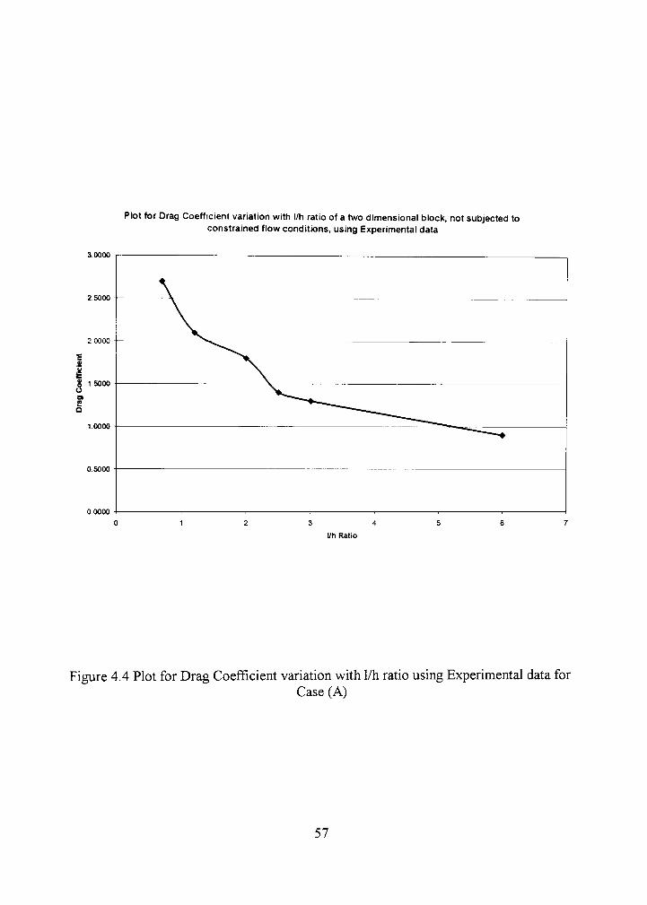
Plot for Drag Coefficient variation with l/h ratio of a two dimensional block, not subjected to constrained flow conditions, using Experimental data
•E
1.5000
S
a
0.0000
Figure 4.4 Plot for Drag Coefficient variafion with l/h rafio using Experimental data for Case (A)
57
PkJt for Drag Coefficient variation with l/h ratio of a two dimensional block, not subjected to constrained flow conditions, using PHOENICS data
1 2600
l/h Ratio
Figure 4.5 Plot for Drag coefficient variation with l/h rafio using PHOENICS data for Case (A)
58
Plot for Drag Coefficient variation with l/h ratio of a two dimensional block, not subjected to constrained flow conditions, using AIRFL03D data
2.5000
Figure 4.6 Plot for Drag Coefficient variation with l/h ratio using AIRFL03D data for Case (A)
59
Plot for Blockage Correction Equation using PHOENICS data and Experimental Data
1 4000
00000
1,0000 1,5000 2,0000
Experimental Drag Coefficient
2,5000
Figure 4.7 Plot for Drag Correction using PHOENICS data for Case (A)
60
Plot for Blockage Correction Equation using AIRFL03D data and Experimental Data
3,0000
2 5000
1 2.0000
E 1.5000 Q Q
< 1 0000
-
•
« • ^ -
y=0,2419x + 1,7533
• -*
0.0000 1,0000 1,5000 2,0000
Experimental Drag Coefficient
3,0000
Figure 4.8 Plot for Drag Correction using AIRFL03D data for Case (A)
61
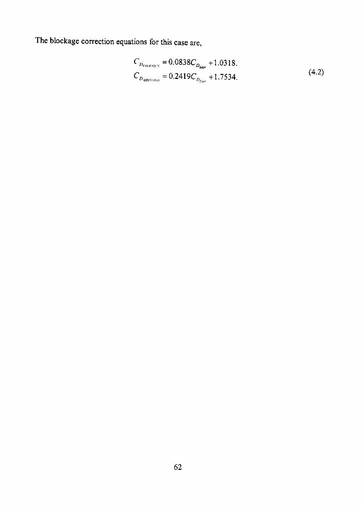
The blockage correction equations for this case are,
^'W«.,.=0-0838C^^,+1.0318.
<^o..,„.,„=0-2419Q, +1.7534. " " ^
62
i l CaseXB}Jfvv;oJDimerisioriaJ I low around a rectangular section subjected to a constrained flow field in a wind
Iunnci test section
The computational domain in this case also, is vertically symmetric. A Constant
velocitv profile is applied at the inlet. This produces a vertically symmetric flow structure
around the blockage. For this reason, the pressure signature and the velocity profile are
plotted for the data acquired along a line drawn longitudinally in the flow direction,
verticalh' positioned on top ofthe rectangular blockage, i.e., along line AB in Figure 4.1.
Results hav e been obtained from both PHOENICS and AIRFL03D.
From the plot for pressure signature using PHOENICS data, one can see a gradual
increase in the positiv e pressure from the test section entrance, up to approximately one-
third blockage length, ahead of the blockage. Thereafter, the pressure takes a rapid
increase till the starting edge of the blockage. Beyond this point, it steeply falls down
below zero pressure mark, through a short distance on the blockage. Then an increase in
the pressure is seen, which stabilizes along the surface ofthe blockage and a little beyond
the blockage. Past that point, the pressure further increases and then stabilizes at zero
pressure way up to the exit of the test section. An insignificant variation in pressure is
seen for varying blockage ratios; but along the surface ofthe blockage and a little beyond
it, the magnitude of pressure decreases with increasing blockage ratio. The same
explanation does not hold good for the data obtained from AIRFL03D.
According to AIRFL03D, the pressure at the test section entrance is
approximately at zero mark. This pressure as detected in PHOENICS increases up to a
distance, approximately one-third the blockage length ahead of the blockage. Then the
63
pressure stcepiv drops beyond this up to a point a little beyond the blockage starting
point. Then the pressure again increases along the blockage surface, but does not remain
stable. Be>ond the end point ofthe blockage, the pressure drops again in the wake region
and suddenh increases beyond the wake region. The pressure beyond this gradually
decreases and stabilizes at the test section exit. A considerable variation can be seen in
the pressure signature can be seen w ith the change in the blockage ratio. All along the
longitudinal distance considered, at any point, the pressure signature magnitude decreases
w ith increase in the blockage ratio. The variations in pressure signature can be clearly
seen in Figures 4.9 and 4.11.
From the plot in Figure 4.10, the velocity profile from PHOENICS data, it can be
seen that the v elocity magnitude decreases gradually up to a point in front of the
blockage. A little distance beyond the starting point ofthe blockage, a minute increase in
the \ elocitv is seen; but beyond this point, it decreases again along the blockage length,
with a little increase, in the wake region beyond the blockage. Past the wake, the velocity
gradually increases and stabihzes fmally at the exit. There is not much variation seen in
the V elocity with varying blockage ratio. On the other hand, in case ofthe velocity profile
obtained from AIRFL03D, Figure 4.12, there is a constant decrease in the velocity till
the starting point of the blockage. The velocity then, suddenly increases and the trend
continues along the blockage and into the wake region, where the velocity is highest in
magnitude. Beyond the wake region, the velocity drops suddenly and with a gradual
increase, it stabilizes as the exit ofthe test section approaches.
64
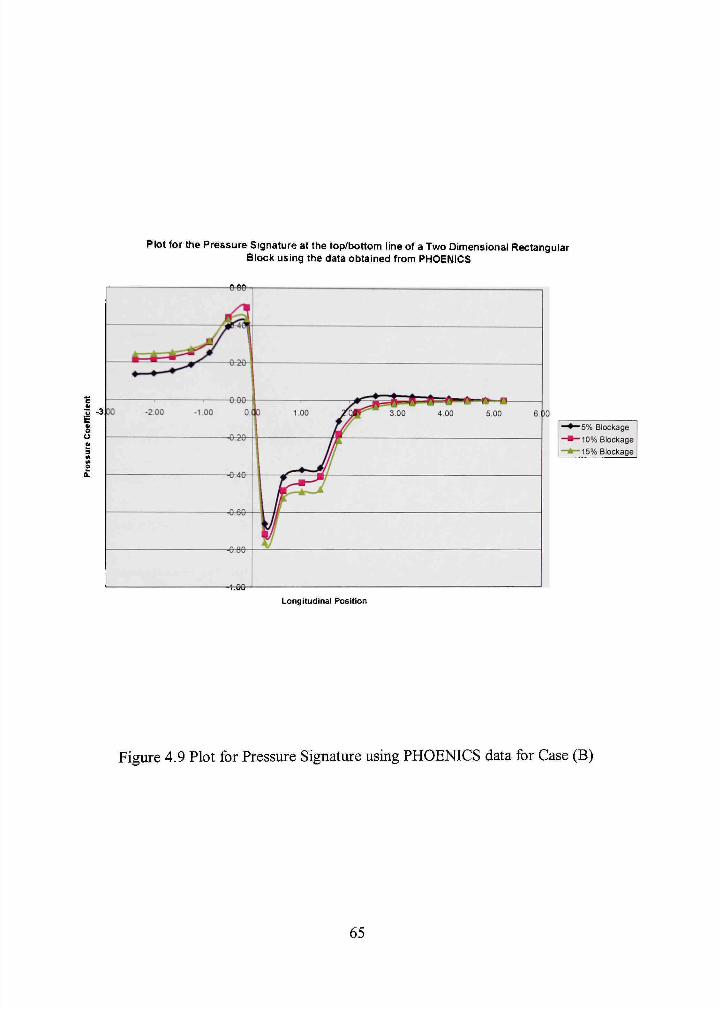
Plot for the Pressure Signature at the top/bottom line of a Two Dimensional Rectangular Block using the data obtained from PHOENICS
- 3 :
-tTflfr
Longitudinal Position
- 5 % Blockage
-10% BloGl<age
-15%Blocl<age
Figure 4.9 Plot for Pressure Signature using PHOENICS data for Case (B)
65
Plot for the Velocity Profile at the top/bottom line of a Two Dimensional Rectangular Block using the data obtained from PHOENICS
-3.00 -2.00 0,00 1,00 2,00
Longitudinal Position
3,00 4,00 5.00
• 5 % Blockage
-10% Blockage
-15% Blockage
Figure 4.10 Plot for Velocity Profile using PHOENICS data for Case (B)
66
Plot for the Pressure Signature at the top/bottom line of a Two Dimensional Rectangular Block using the data obtained from AIRFL03D
-3 DO
o U
-4-6fr
Longitudinal Position
-5% Blockage -10% Blockage -15% Blockage
Figure 4.11 Plot for Pressure Signature using AIRFL03D data for Case (B)
67
Plot for the Velocity Profile at the top/bottom line of a Two Dimensional Rectangular Block using the data obtained from AIRFL03D
-1-se-
0 60
-6-46-
- « ^ S -
0 00 -3,00 -2 00 -1,00 0,00 1,00 2,00 3,00 4,00
Longitudinal Position
-5% Blockage
-10% Blockage
-l5%iBlockage
5,00 6,00
Figure 4.12 Plot for Velocity Profile using AIRFL03D data for Case (B)
68
The increase in pressure in front ofthe blockage, is caused due to the stagnation
ot flow at the front ofthe blockage. The formation of stagnation point causes an increase
in the pressure in its v icinity, gradually decreasing to attain normal value, away from the
point. The steep decrease in pressure, immediately after that, is caused due to the sudden
change in direction of flow and the increase in velocity at the front edge ofthe blockage.
Beyond this point, the pressure is not much effected by the change in flow, due to which,
a gradual increase and subsequent stabilization of pressure is seen, as predicted by
PHOENTCS. But bevond the blockage, in the vicinity of the wake, AIRFL03D has
predicted a sudden dip in pressure, which shows that the pressure is effected by the
sudden decrease in velocity in the wake region. This might be attributed the Kato and
Launder K-s model, used in AIRFL03D code.
The velocity vector plot for this case (See Appendix), shows that the flow
separation occurs at the top ofthe block and reattaches at a point around the midway of
the blockage. PHOENICS does not produce a wake bubble at the top of the blockage.
This might be because the K-s model with wall conditions was not able to predict it. The
Kato and Launder model used in AIRFL03D has, predicted the wake as indicated in (27).
It can also be seen that the K-s model used in PHOENICS, shows the effect of the wake
even at the test section exit, which is not the same with AIRFL03D. The wake is
confined to a very small region behind the blockage and the flow past the wake tends to
get normal.
The drag coefficients are plotted for different blockage ratios. Drag coefficients
obtained from both PHOENICS and AIRFL03D are plotted for variation with Blockage
69
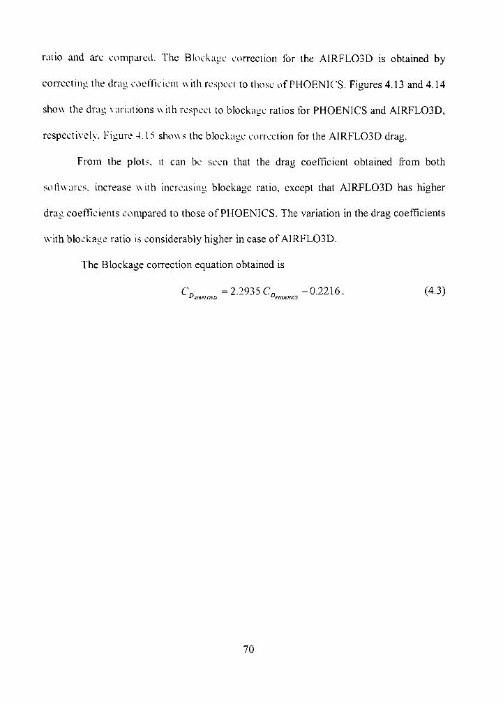
ratio and arc compared. The Blockage correction for the AIRFL03D is obtained by
correcting the drag coefficient with respect to those of PHOENICS. Figures 4.13 and 4.14
show the drag v ariations w ith respect to blockage ratios for PHOENICS and AIRFL03D,
respectivelv. Figure 4.15 shows the blockage correction for the AIRFL03D drag.
From the plots, it can be seen that the drag coefficient obtained from both
sotlwarcs. increase with increasing blockage ratio, except that AIRFL03D has higher
drag coefTicients compared to those of PHOENICS. The variation in the drag coefficients
w ith blockage ratio is considerably higher in case of AIRFL03D.
The Blockage correction equation obtained is
C„ = 2.2935 C„ -0.2216. (4.3)
70
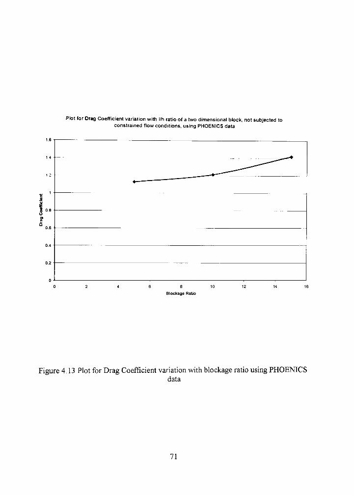
Ptot for Drag Coefficient variation with l/h ratio of a two dimensional block, not subjected to constrained flow conditions, using PHOENICS data
Blockage Ratio
Figure 4.13 Plot for Drag Coefficient variation with blockage rafio using PHOENICS data
71
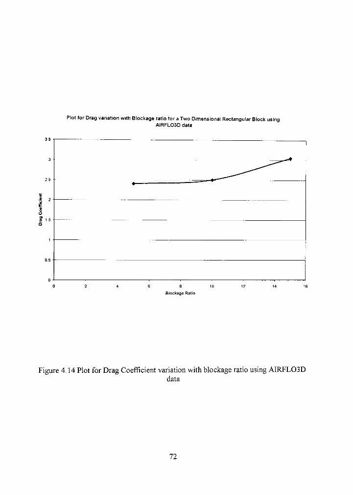
Plot for Drag variation with Blockage ratio for a Two Dimensional Rectangular Block using AIRFL03D data
a 10 Blockage Ratio
Figure 4.14 Plot for Drag Coefficient variafion with blockage rafio using AIRFL03D data
72
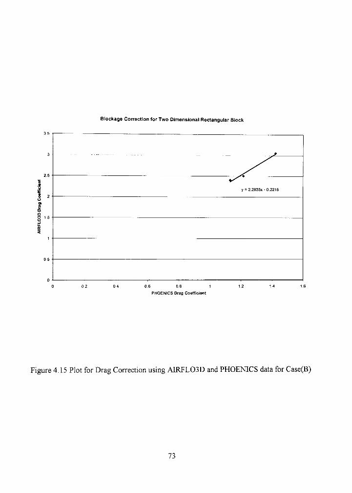
Blockage Correction for Two Dimensional Rectangular Block
y = 2.2935x-0,2216
5 Q a S '' _i u. <
02 04 0,6 0,8 1 PHOENICS Drag Coefficient
Figure 4.15 Plot for Drag Correction using AIRFL03D and PHOENICS data for Case(B)
73
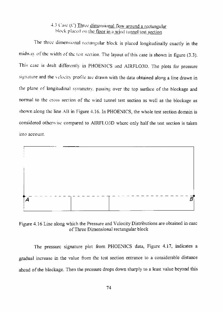
4.3 Case (C) Three cfirnensional flow around a rectangular block placed on the floor in ajwjnd tunnel test section
The three dimensional rectangular block is placed longitudinally exactly in the
midwav ofthe width ofthe test section. The layout of this case is shown in figure (3.3).
This case is dealt differently in PHOENICS and A1RFL03D. The plots for pressure
signature and the velocitv profile are drawn with the data obtained along a line drawn in
the plane of longitudinal svinmetry. passing over the top surface ofthe blockage and
normal to the cross section ofthe wind tunnel test section as well as the blockage as
shown along the line .AB in Figure 4.16. In PHOENICS, the whole test section domain is
considered otherwise compared to AIRFL03D where only half the test section is taken
into account.
B
Figure 4.16 Line along which the Pressure and Velocity Distributions are obtained in case of Three Dimensional rectangular block
The pressure signature plot from PHOENICS data. Figure 4.17, indicates a
gradual increase in the value from the test section entrance to a considerable distance
ahead ofthe blockage. Then the pressure drops down sharply to a least value beyond this
74
point until a point just after the front wall of the blockage is reached. From this, the
pressure again rises to an intermediate level and partially stabilizes over the blockage
surtace. The pressure is found to decrease again a little at the end ofthe blockage, but
increases in the w ake region. The pressure past the wake is found to gradually tending to
stabilize. For the three blockage ratios, beyond the front wall of the blockage, the
pressure is found to decrease w ith increasing blockage ratio, except at the exit, that the
three cases end up at zero pressure.
.\s in the case of .\IRFL03D, refer Figure 4.19, the pattern of the pressure
signature matches v\ith that of the PHOENICS and that the pressure decreases with
increasing blockage ratio. But the difference between the two is that, beyond the wake
region the difference in pressure magnitude is seen to exist till the test section exit point.
If one looks at the \elocity profile for both PHOENICS and AIRFL03D, they
match V er\ w ell in most of the regions. The velocity is found to gradually decrease in
magnitude through the entrance to the vicinity of the stagnation point. But at the front
edge region, a hump in the velocity profile is seen followed by a considerable reduction
in magnitude which ahnost dies down to zero in the midway ofthe blockage length. The
velocity then rises gradually beyond that. With the little change in course ofthe profile at
the wake region, the velocity tends to attain the initial velocity conditions at exit.
The velocity profile is found to have not effected by the change in the blockage
ratio in case of AIRFL03D. In case of PHOENICS, the velocity is found to decrease with
increasing blockage ratio, in the regions just beyond the front face ofthe blockage and
beyond the rear face ofthe blockage. Figures 4.18 and 4.20 depict the velocity profiles.
75
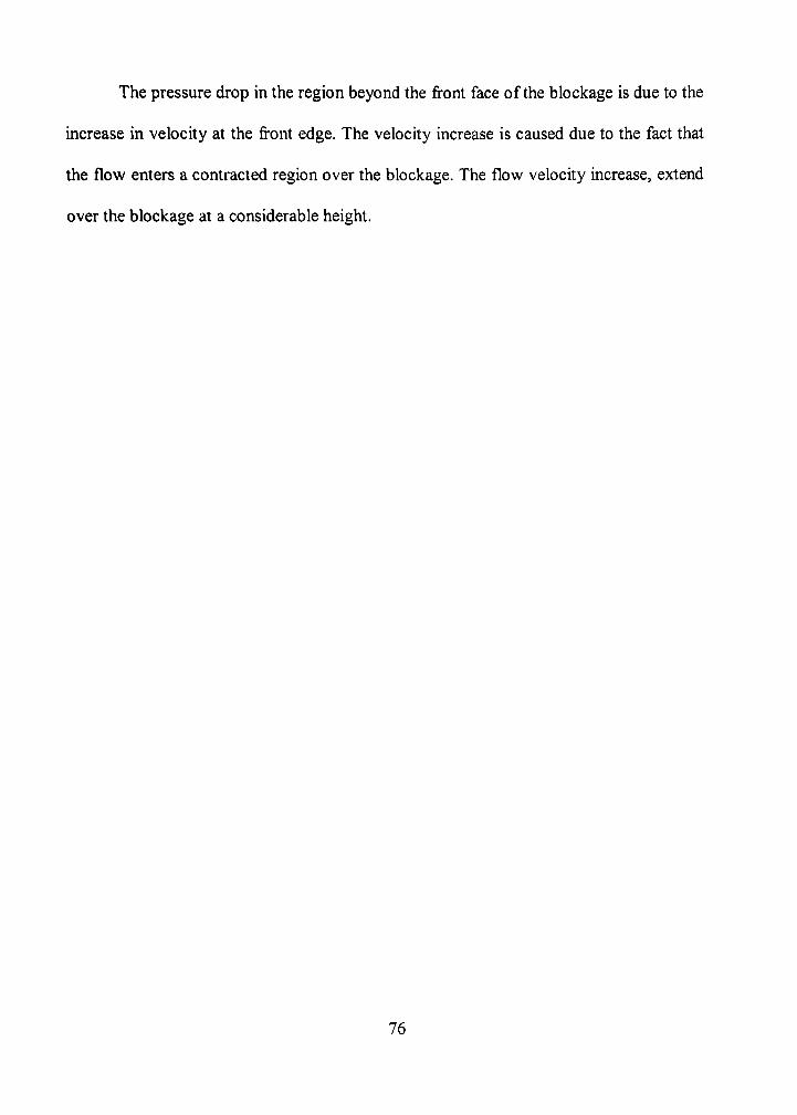
The pressiu-e drop in the region beyond the front face ofthe blockage is due to the
increase in velocity at the front edge. The velocity increase is caused due to the fact that
the flow enters a contracted region over the blockage. The flow velocity increase, extend
over the blockage at a considerable height.
76
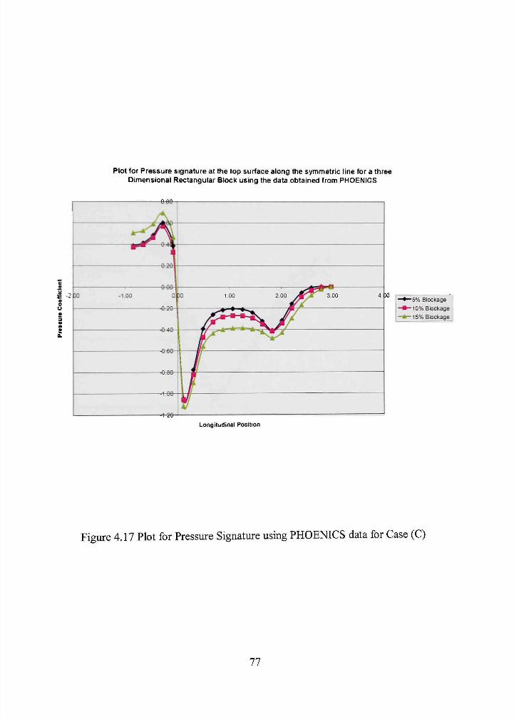
Plot for Pressure signature at the top surface along the symmetric line for a three Dimensional Rectangular Block using the data obtained from PHOENICS
-6^*
-5%) Blockage -10% Blockage -15% Blockage
Longitudinal Position
Figure 4.17 Plot for Pressure Signature using PHOENICS data for Case (C)
77
Ptot for Velocity Profile at the top surface along the symmetric line for a Three Dimensional Rectangular Block using the data obtained from PHOENICS
-«e-
u
« >
-2.00 -1.00
- 5 % Blockage
-10% Blockage
-15% Blockage
0.00 1,00
Longitudinal Position
Figure 4.18 Plot for Velocity Profile using PHOENICS data for Case (C)
78
- : 50
Plot for Pressure Signature at the top surface along the symmetric line for a three Dimensional Rectangular Block using the data obtained from A1RFL03D
4,10
-5% Blockage -10% Blockage -15% Blockage
Longitudinal Position
Figure 4.19 Plot for Pressure Signature using AIRFL03D data for Case (C)
79
Plot for Velocity Profile at the top surface along the symmetric line for a three Dimensional Rectangular Block using the data obtained from AIRFL03D
-2,00 -1,00 0,00 1,00
Longitudinal Position
-5% Blockage
-10% Blockage
-15% Blockage
Figure 4.20 Plot for Velocity Profile using AIRFL03D data for Case (C)
80
The reduction in the flow velocity just over the blockage may be due to the
formation of boundiu-y laver at the top surface. In PHOENICS, the separation of this
boundarv laver occurs farther on the blockage surface (rear end of the blockage)
compared to the case in .•\1RFL03D. As a result, an early rise in flow velocity on the
blockage is observed in .•\1RFL03D. The Kato and Launder model, which avoids over-
prediction ofthe kinetic energy, which in turn is the energy due to the velocity ofthe
fluid particles, should be the reason for the early rise in the velocity from minimum. The
low Re>iiolds number K-e model used in PHOENICS does not over-predict the results as
in the ordinar\ K-s model. But it provides a more realistic flow structure.
The pressure signature is observed to take a small dip again at the rear end ofthe
blockage. This can be attributed to the flow separation that occurs at the region in case of
PHOEMCS. The same type of dip is observed in AIRFL03D much earlier, to which the
explanation is as above.
The faint dip in the velocity magnitude at the rear edge of the blockage is
because; the region beyond this is the vicinity of the wake bubble. Beyond the wake
bubble, the velocity tends to pick, which is caused due to the effect of previous velocity
increase at the front edge. This can be seen in the velocity vector plot provided in the
Appendix.
The drag coefficients are plotted for different blockage ratios. Drag coefficients
obtained from both PHOENICS and AIRFL03D are plotted for variation with Blockage
ratio and are compared. The Blockage correction for the AIRFL03D is obtained by
correcting the drag coefficient with respect to those of PHOENICS. Figures 4.21 and 4.22
81
show the drag variations with respect to blockage ratios for PHOENICS and AIRFL03D,
respectively. From the plots, it can be seen that the drag coefficient obtained from both
softwares, increase with increasing blockage ratio, except that AIRFL03D has higher
drag coefficients compared to those of PHOENICS. The variation in the drag coefficients
with blockage ratio is considerably higher in case of AIRFL03D.
The Blockage correction equations are taken as quadratic fit for the drag
coefficients plotted against blockage ratio. The equations are in the form
C. =0.0012 '^AIKFLOID
U.^' vA-v
+ 0.0269 u vAy
+ 1.511. (4.4)
Cr = 0.0016 ^A.^'
\^wj -0.0241
'A^
vAy + 1.098. (4.5)
From the above equations, it can be seen that the drag variation with blockage
ratio is almost linear.
82
Ptot for Drag variation with Blockage ratio for a Three Dimensional Rectangular Block using PHOENICS data
0,6
y = 0.0016x -0,0241x+ 1,096
8
Blockage Ratio
10
Figure 4.21 Plot for Drag Coefficient varying with Blockage Ratio using PHOENICS
data
83
Ptot for Drag variation with Blockage ratio for a Three Dimensional Rectangular Block using A1RFL03D data
0 5
8 10
Blockage Ratio
14 16
Figure 4.22 Plot for Drag Coefficient varying with Blockage Ratio using AIRFL03D
data
84
4.4 Case_(D) Three Dimensional flow around a top-front edg e tapereci rectanajlarlilockaue placed close to the floor
of a wind tunnel test section
In this case, the blockage is located at a certain height above the wind tunnel test
section floor. The flow is asvmmetric vertically which is not the same situation as in
cases (.V) and (B). So the pressure signatures and velocity profiles along the upper as well
as the lower surtaces ofthe blockage are needed to be analyzed. The lines along which
the plots are drawn are placed along the plane of longitudinal symmetry and normal to
the cross sectional area ofthe test section.
A
C
B
D.
Figure 4.23 Lines along which the Pressure and Velocity Distributions are obtained in case of Three Dimensional top-edge tapered block
The pressure signature along the top ofthe blockage is analyzed first i.e., line AB
in Figure 4.23. In this case, the trend in the pressure signature profiles obtained from both
PHOENICS and AIRFL03D is same. But in front ofthe blockage front end, the pressure
rise in PHOENICS is observed to be more than that in AIRFL03D. Even the drop in
pressure beyond that point above the slant surface is more compared to that in
85
AIRFL03D. The signature above the flat surface of the blockage is observed to be
stabilizing a little. But bevoiul the rear end of the blockage, there is a dip in the pressure
and a gradual rise, attaining a stabilized state at the test section exit. The pressure at the
test section exit is found to be zero, iirespective of the blockage ratio, in the case of
PHOENICS, But there is a considerable difference in the pressure signature with
variation in blockage ratio in case of .•\IRFL03D. The pressure is observed to decrease
with increase in the blockage ratio. From the test section entrance to the blockage front
end. the pressure variation w ith blockage is not observed to as significant extent. Figures
4.24 and 4.26 depict the variations in pressure signature.
The V elocitv profiles for PHOENICS and AIRFL03D differ to as certain extent.
.\ccording to the PHOENTCS data. Figure 4.25, a velocity drop is seen in the vicinity of
the stagnation point at the blockage front end. Beyond that, an increase is seen in velocity
up to the intersection ofthe slanted surface and the top horizontal surface ofthe blockage.
Then again, velocity decreases gradually till the blockage rear end. Then a sudden
decrease in the velocity in the wake region, followed by stabilization of flow at the test
section exit, is observed.
The flow model is more detailed in AIRFL03D, Figure 4.27. The velocity drops
down up to the front end ofthe blockage. Past this point, due to an increase in the flow
velocity at the front edge, there is a corresponding increase in the flow above this point.
But again, due to the formation ofthe boundary layer on the slant surface, velocity drop
in the region occurs. At the point of intersection of the slant surface and the horizontal
plane at the top, velocity increases, due to the change in flow direction at the point and
86
tlovv contraction bevond it. However the flow contraction is observed to be gradual,
which does not elTect much, the increasing trend ofthe velocity, till the rear end ofthe
blockage is reached. But at the v icinity ofthe wake bubble, the velocity drops down and
before the exit is reached, the flow tends to stabilize.
87
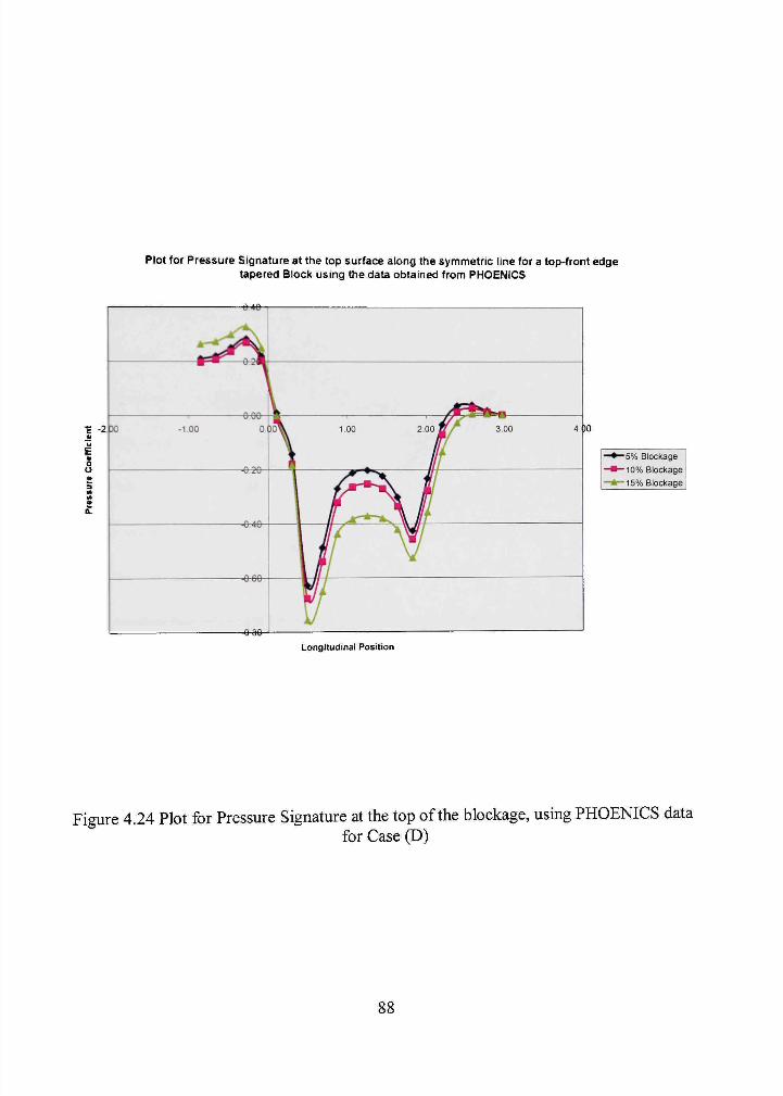
Plot for Pressure Signature at the top surface along the symmetric line for a top-front edge tapered Block using the data obtained from PHOENICS
-2 30
-5% Blockage
-10% Blockage
-15% Blockage
Longitudinal Position
Figure 4.24 Plot for Pressure Signature at the top ofthe blockage, using PHOENICS data for Case (D)
88
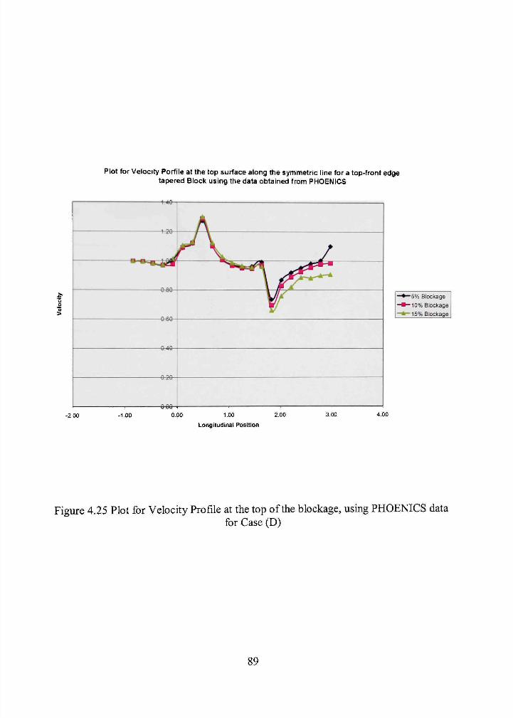
Plot for Velocity Porfile at the top surface along the symmetric line for a top-front edge tapered Block using the data obtained from PHOENICS
O
>
-5% Blockage
-10% Blockage
-15%) Blockage
-2 00 -1,00 0,00 1.00
Longitudinal Position
2,00
Figure 4.25 Plot for Velocity Profile at the top ofthe blockage, using PHOENICS data for Case (D)
89
Plot for Pressure Signature at the top surface along the symmetric line for a top-front edge tapered Block using the data obtained from AIRFL03D
• 50
Longitudinal Position
3 )0
-5% Blockage
-10%> Blockage
-I5%i Blockage
Figure 4.26 Plot for Pressure Signature at the top ofthe blockage, using AIRFL03D data for Case (D)
90
Plot for Velocity Profile at the top surface along the symmetric line for a top-front edge tapered Block using the data obtained from AIRFL03D
- 5 % Blockage
-10% Blockage
-15% Blockage
-1.50 -0,50 0,00 0,50 1,00
Longitudinal Position
Figure 4.27 Plot for Velocity Profile at the top ofthe blockage, using AIRFL03D data for Case (D)
91
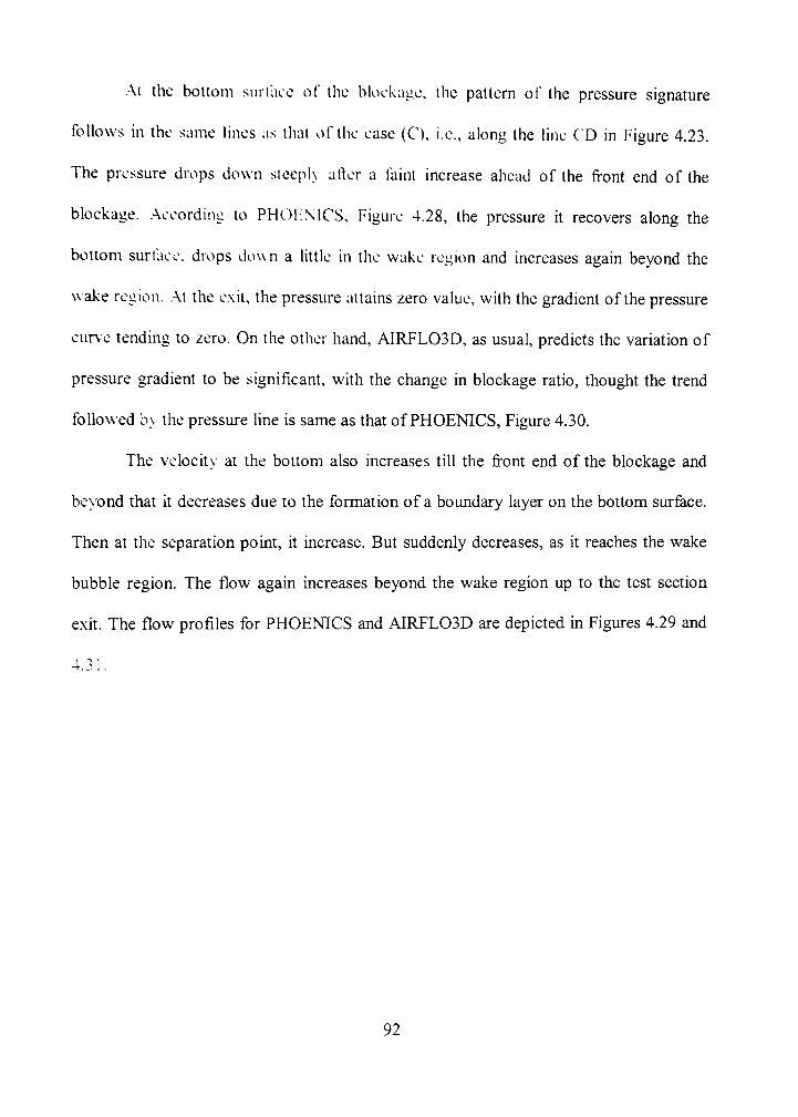
.•\t the bottom surface of the blockage, the pattern of the pressure signature
follows in the same lines as that ofthe case (C), i.e., along the line CD in Figure 4.23.
The pressure drops down steepiv after a faint increase ahead of the front end of the
blockage. According to P H 0 1 : N I C S , Figure 4.28, the pressure it recovers along the
bottom surtace, drops down a little in the wake region and increases again beyond the
w ake region. .\t the exit, the pressure attains zero value, with the gradient ofthe pressure
cur\e tending to zero. On the other hand, A1RFL03D, as usual, predicts the variation of
pressure gradient to be significant, with the change in blockage ratio, thought the trend
followed b\ the pressure line is same as that of PHOENICS, Figure 4.30.
The velocitv at the bottom also increases till the front end of the blockage and
bevond that it decreases due to the formation of a boimdary layer on the bottom surface.
Then at the separation point, it increase. But suddenly decreases, as it reaches the wake
bubble region. The flow again increases beyond the wake region up to the test section
exit. The flow profiles for PHOENICS and AIRFL03D are depicted in Figures 4.29 and
4.31.
92
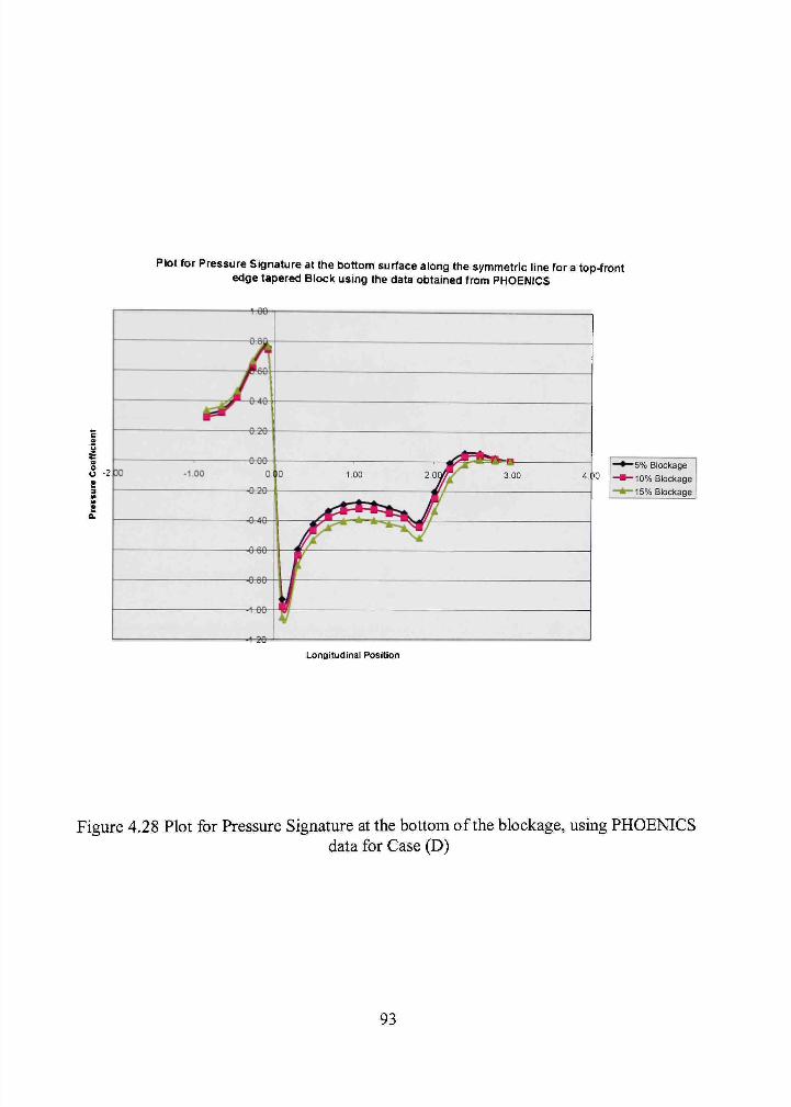
Plot for Pressure Signature at the bottom surface along the symmetric line for a top-front edge tapered Block using the data obtained from PHOENICS
(3 -2 X -5% Blockage -10% Blockage -15% Blockage
Longitudinal Position
Figure 4.28 Plot for Pressure Signature at the bottom ofthe blockage, using PHOENICS data for Case (D)
93
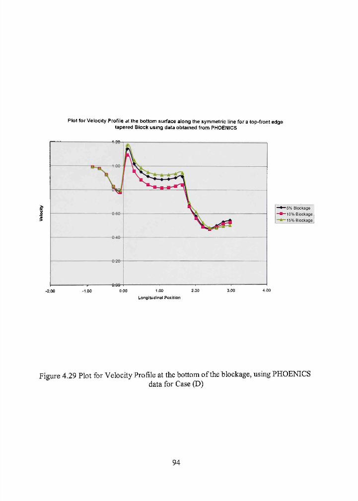
Ptot for Velocity Profile at the bottom surface along the symmetric line for a top-front edge tapered Block using data obtained from PHOENICS
•5% Blockage
-10% Blockage
-15% Blockage
-1.00 0,00 1,00 2,00
Longitudinal Position
4,00
Figure 4.29 Plot for Velocity Profile at the bottom ofthe blockage, using PHOENICS data for Case (D)
94
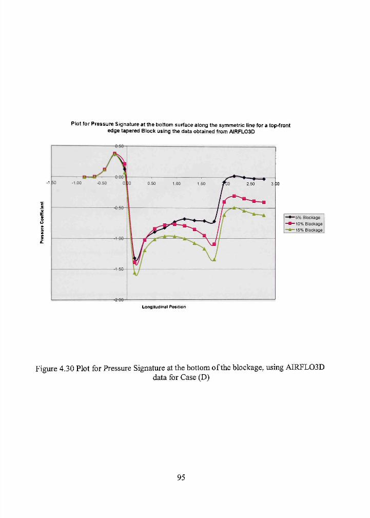
•1 50
Plot for Pressure Signature at the bottom surface along the symmetric line for a top-front edge tapered Block using the data obtained from AIRFL03D
-2-9&
Longitudinal Position
3 )0
-5% Blockage
-10% Blockage
-15% Blockage
Figure 4.30 Plot for Pressure Signature at the bottom ofthe blockage, using AIRFL03D data for Case (D)
95
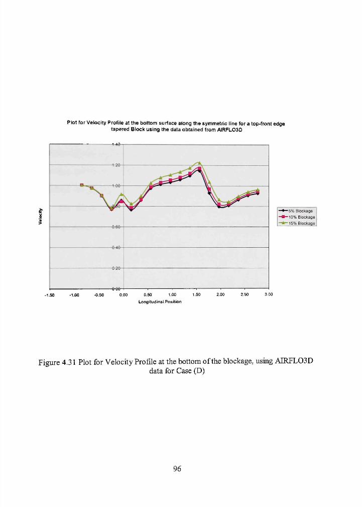
Ptot for Velocity Profile at the bottom surface along the symmetric line for a top-front edge tapered Block using the data obtained from AIRFL03D
1 40
-*6e-
0 40
-6^6-
• ^—5% Blockage
- •—10% Blockage
-t.~-15% Blockage
-1.50 -1.00 0.50 1,00
Longitudinal Position
2,00
Figure 4.31 Plot for Velocity Profile at the bottom ofthe blockage, using AIRFL03D data for Case (D)
96
The drag coefTicients are plotted for different blockage ratios. Drag coefficients
obtained from both PHOI-NICS and A1RFL03D are plotted for variation with Blockage
ratio and are compared. The Blockage correction for AIRFL03D is obtained by
correcting the drag coetTicient w ith respect to those of PHOENICS. The Figures 4.32 and
4.33 show the drag variations with respect to blockage ratios for PHOENICS and
.\1RFL03D, respectivel\. From the plots, it can be seen that the drag coefficient obtained
from both softwares, increase w ith increasing blockage ratio, except that AIRFL03D has
higher drag coefticients compared to those of PHOENICS. The variation in the drag
coetTicients v\ith blockage ratio is considerably higher in case of AIRFL03D.
The Blockage correction equations are taken as quadratic fit for the drag
coefficients plotted against blockage ratio. The equations are in the form
Cr, =0.0048 'Ay V^^wy
0.0214 'A^
v^wy + 1.091 (4.6)
C„ = 0.0003 '^PHOENICS
u ^' /^J
+ 0.0157 'A^
v^H-y + 0.5698. (4.7)
From the above equations, it can be seen that the drag variation with blockage
ratio is almost linear.
97
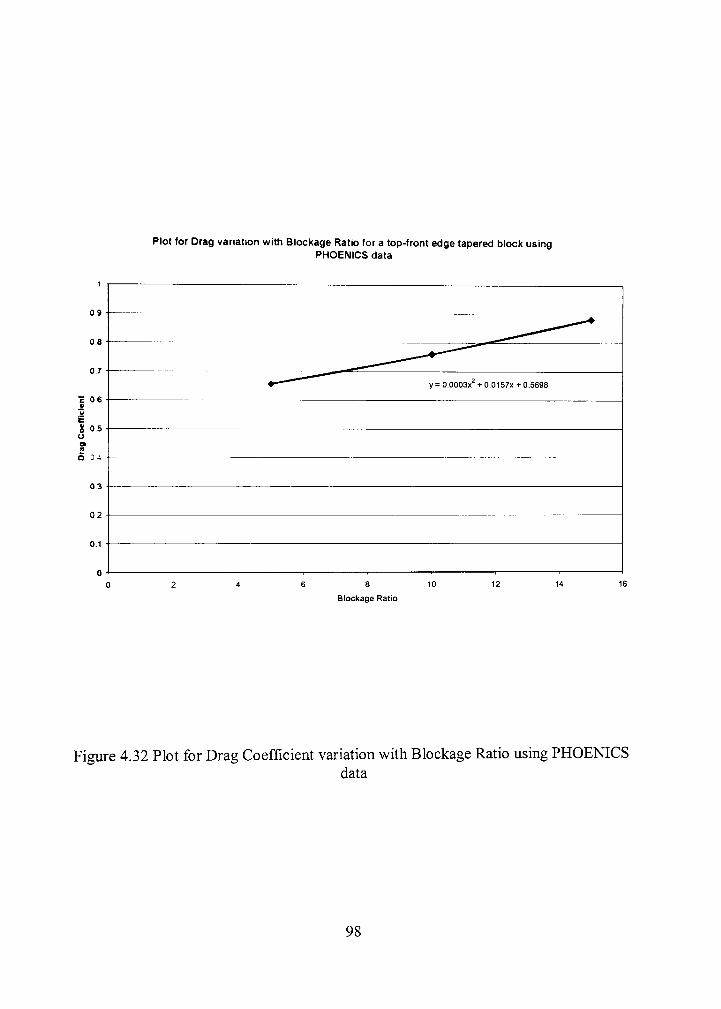
0 9 —
0,7
c 0 6
£ g 05 o o n O 04 —
0.3
0 2
Plot for Drag variation with Blockage Ratio for a top-front edge tapered block using PHOENICS data
y= O.OOOax + 0,0157x + 0,5698
12
Blockage Ratio
Figure 4.32 Plot for Drag Coefficient variation with Blockage Ratio using PHOENICS data
98
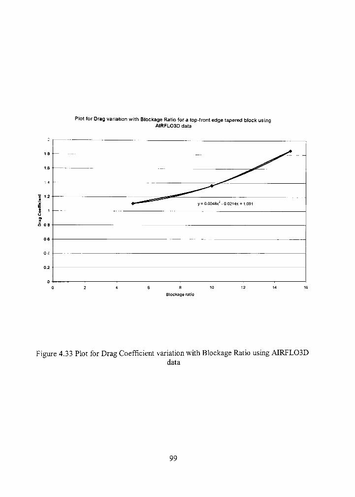
18
1.2
Plot for Drag variation with Blockage Ratio for a top-front edge tapered block using AIRFL03D data
y = 0,0048x - 0,0214x + 1,091
0.2
8
Blockage ratio
Figure 4.33 Plot for Drag Coefficient variation with Blockage Ratio using AIRFL03D data
99
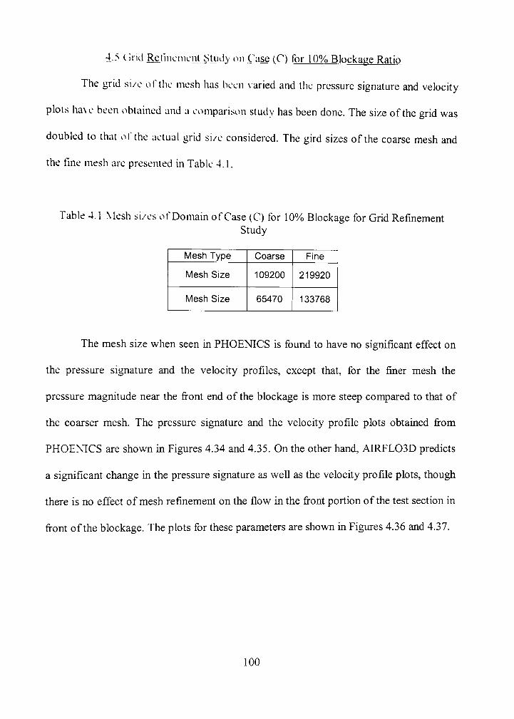
4.5 Crid Rennement Study on Qise (C) for 10% Blockaue Ratio
The grid si/e ofthe mesh has been varied and the pressure signature and velocity
plots have been obtained and a comparison study has been done. The size ofthe grid was
doubled to that ofthe actual grid si/e considered. The gird sizes ofthe coarse mesh and
the fine mesh are presented in Table 4.1.
Table 4.1 Mesh si/es of Domain of Case (C) for 10% Blockage for Grid Refinement Study
Mesh Type
Mesh Size
Mesh Size
Coarse
109200
65470
Fine
219920
133768
The mesh size when seen in PHOENICS is found to have no significant effect on
the pressure signature and the velocity profiles, except that, for the finer mesh the
pressure magnitude near the front end of the blockage is more steep compared to that of
the coarser mesh. The pressure signature and the velocity profile plots obtained from
PHOENTCS are shown in Figures 4.34 and 4.35. On the other hand, AIRFL03D predicts
a significant change in the pressure signature as well as the velocity profile plots, though
there is no effect of mesh refmement on the flow in the front portion ofthe test section in
front ofthe blockage. The plots for these parameters are shown in Figures 4.36 and 4.37.
100
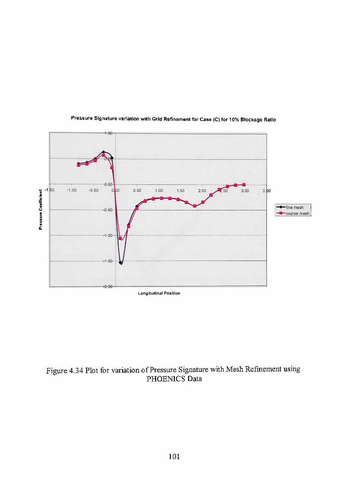
Pressure Signature variation with Grid Refinement for Case (C) for 10% Blockage Ratio
- -1 50
"fine mesh -coarse mesh
Longitudinal Position
Figure 4.34 Plot for variation of Pressure Signature with Mesh Refmement using PHOENICS Data
101
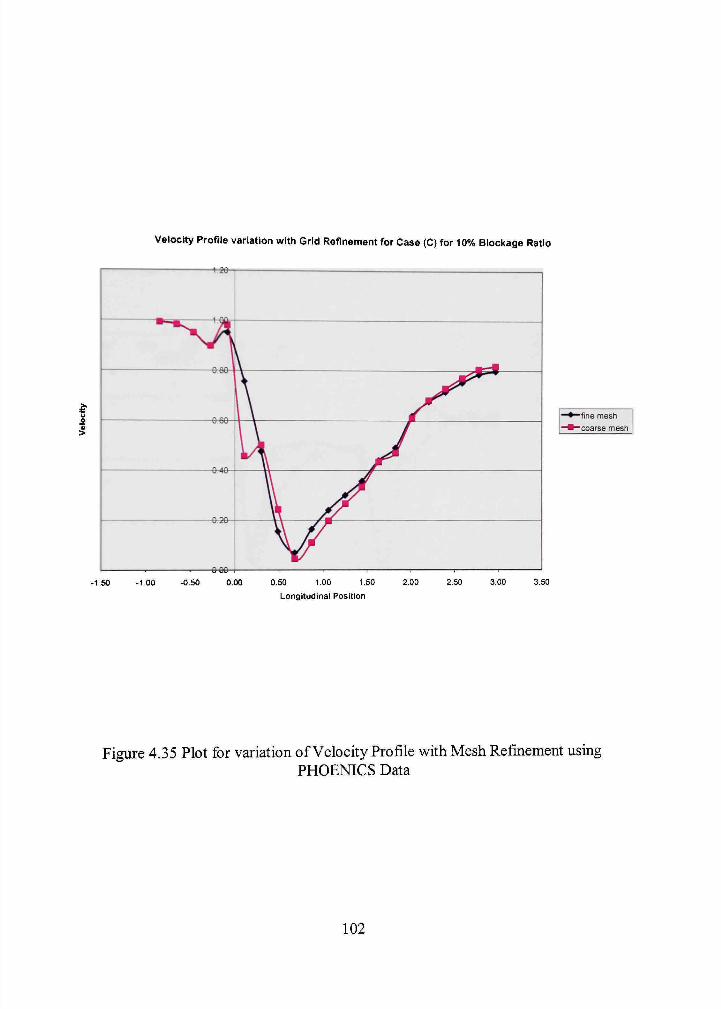
u O
>
Velocity Profile variation with Grid Refinement for Case (C) for 10% Blockage Ratio
•fine mesh
-coarse mesh
-1.50 -1.00 -0,50 0,00 0,50 1.00 1,50
Longitudinal Position
2,00 2,50 3,00 3,50
Figure 4.35 Plot for variation of Velocity Profile with Mesh Refmement using PHOENICS Data
102
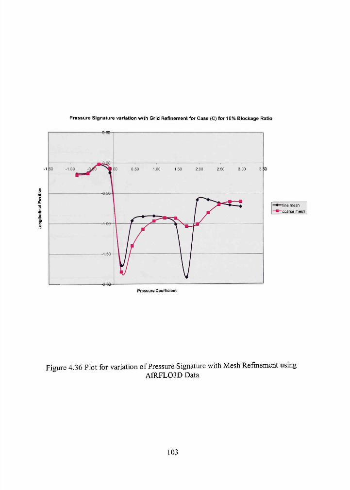
Pressure Signature variation with Grid Refinement for Case (C) for 10% Blockage Ratio
e-56-
-1 50 00 0,50 1,00 1,50 2,00 2.50 3 00 3 50
-200
Pressure Coefficient
-fine mesh
-coarse mesh
Figure 4.36 Plot for variation of Pressure Signature with Mesh Refmement using AIRFL03D Data
103
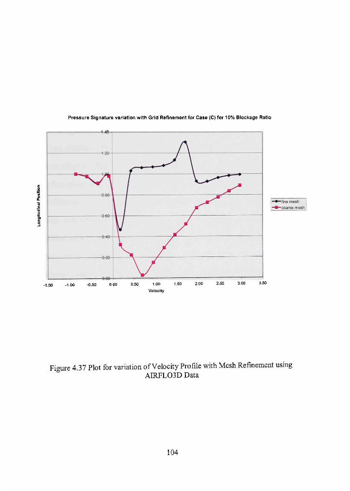
Pressure Signature variation with Grid Refinement for Case (C) for 10% Blockage Ratio
-Mfr
-fine mesh -coarse mesh
-1,50 -1.00 -0.50 0.00 0,50 1,00 1,50 Velocity
2,00 2,50 3,00 3,50
Figure 4.37 Plot for variation of Velocity Profile with Mesh Refmement using AIRFL03D Data
104
CHAPTER 5
C^ONCLLISIONS AND FUTURE WORK
CFD flow simulations have successfully been performed using PHOENICS and
.\1RFL03D for different blockages placed in wind tunnel test sections. The effects of
wind tunnel blockages on the pressure and velocity distributions along the flow direction
have been predicted. The blockage effects due to varying test section height have been
found to efTect the flow parameters, significantly. Blockage corrections from the drag
correction equations have been proposed for the data obtained from PHOENICS and
.\IRFL03D for both tw o dimensional and three dimensional cases. The drag coefficient
variation w ith blockage / /; ratio, in case of a two dimensional unconstrained flow,
reasonably agree w ith the experimental results. The AIRFL03D drag predictions are seen
to have \ielded higher values compared to PHOENICS and the experimental drag
coefficients. AIRFL03D is also found to show significant variations in the drag
coefficients compared to PHOENICS. The blockage correction equations obtained,
pro\ide a good correlation for drag coefficient and the test section height. The velocity
vector plots provide as good source for differentiating the turbulence models used in
PHOENTCS and AIRFL03D. The grid independent study performed predicted a
neghgible influence of mesh size on the results obtained by PHOENICS but the results
obtained from AIRFL03D have a significant effect due to mesh refinement.
Further study is necessary for determining the reason for higher drag predictions
in AIRFL03D. The computational experiments conducted in this work can be extended
105

to a wide range of blockage geometries. As a part of future work, similar type of
experiments if conducted on the blockage geometries used by MIRA, would provide a
strong basis for future development in the study of blockage effects involved in wind
tuimel testing on automobiles. The study can also be extended to determine the
dependence of blockage effects on mesh shape, unsteady conditions and different
velocity profiles.
106
REFERENCES
1. Anonv mous, Wikimedia Foundation, Inc., Wikipedia. "Wind Tunnel," Retrieved March I"', 2()(U, from http://en.wikipcdia.org/wiki/WindJunnel
2. .\nonvnious, Infoplease. Information Please, Fact Monster, and the Information Please Almanac Copvright <-i 2()()() 2004 Pearson Education, publishing as Infoplease. AN ind Tunnel," Accessed March 17, 2004, from http:''wWW .infoplease.com ced sci/A0852448.html
3. "Closed-Tesi-Section Wind Tunnel Blockage Corrections for Road Vehicles." SAE International. SP-1176
4. Filippone, .A... (1999-2004), "Advanced Topics in Aerodynamics." Accessed .March 17, 2004. from http://aerodyn.org/WindTurmel/wind_tunnel.html
5. Rangaraju, K.G. and Singh, V "Blockage effects on Drag of Sharp-edged Bodies." Journal of Industrial Aerodynamics (1975).
6. .Maskell, E.C. "A theory of the Blockage effect on Bluff Bodies and Stalled Wings in a closed Wind l:^xnne\." ARC R&M 3400, Nov 1968.
7. Thom, A. "Blockage correction in a closed high speed turmel." ARC R&M 2033, \o\- 1943.
8. Herriot, J.C. "Blockage correction for three dimensional flow closed throat Witid tunnel with consideration ofthe effect of compressibility." NACA R 995, 1950.
9. Ramamurthy, A.S. and Ng, CP. "Effect of Blockage on Steady Force CoefTicients."' Journal of Engineering Mechanics. Div., Proc. A.S.C.E., P9(1973) 755-772.
10. Awbi, H.W. 'The investigation of wind tunnel wall interference on bluff body models." Ph.D Thesis, Trent Polytechnic, Nottingham, August 1974.
11. Awbi, H.W. "Wind-Tunnel-Wall Constraint on Two-Dimensional Rectangular-Section Frisms."' Journal of Industrial Aerodynamics, 3 (1978) 285-306.
12. Glauert, H. "Wind tunnel interference on wings, bodies and airscrews." ARC, R+M 1566,1933.
107
13. Mercker, E. "A Blockage Correction for Automotive Testing in a Wind Tunnel with Closed Test Section." Journal oj Wind Eni^iiiccrin^ and Industrial Aerodynamics. :: (['•)Sb) \49-\67.
14. Louis. G.S, "A Streamline Wind-Tunnel Working Section for Testing at High Blockage Ratios." Journal of Wind Enginccriiiii (I'ld Industrial Aerodynamics 9 (DSl) 23-31.
L">. Okajima, A., Yi, D., Saliuda, A.. Nakaiio. f "Numerical study of blockage effects on aerodynamic characteristics of an oscillating rectangular cylinder." Journal of Wind En^.:inccrini: and Indusfrial Aerodynamics. 67&68 (]997) 91-102.
16. William, C.L. "Computation of two-dimensional blocked flow normal to a flat plate." Journal of Wind Engineering and Industrial Aerodynamics, 89 (2001) 493-513.
17. Perzon, S. "On Blockage Effects in Wind Tunnels - A CFD Study" Society of Automobile Engineers. Inc.. 2001-01-0705.
18. Yen, J.C, Martindale. W.R, Duell, E.G, Amette, S.A. "Determining Blockage Correction in CUmatic Wind Tunnel, using CFD." SAE International, 2003-01-0936.
19. Rout, R.K "Unique Correlation Technique for Real-World flow simulation in the v\ind tunnel." Society of Automobile Engineers, Paper 980033.
20. ed. Hucho, W.H. "Aerodynamics of Road Vehicles." 1 ' English Edition, Butterworths, Cambridge, 1987.
21. Yang, Z., Schenkel, M., Fadler, G.J. "Corrections for the Pressure Gradient Effect on Vehicle Aerodynamic Drag." SAE International, 2003-01-0935.
22. Jeffrey, H., Bill, M., Stephen, A. (Jacobs Sverdrup), Jack, W., Stan, W. (Ford Motor Company). "Development of Lift and Drag Corrections for Open Jet Wind Tunnel Tests for an Extended Range of Vehicle Shapes." SAE International, 2003-01-0934.
23. Launder, B.E and Spalding, D.B. "The Numerical Computation of Turbulent Flows." (1974), Computational Mechanics and Engineering, 3, 269-289.
24. Spalding, D.B. and Zhubrin, S.V., " X-Cell: A new algorithm for fluid-flow simulation in PHOENICS." Lectures at PHOENCIS Used Conference, April 1996, Tokyo, Japan. Accessed May 25, 2004, from http ://www. simuserve. com/phoenics/d_po lis/d_enc/x-cell. htm# 1.2
108
25. Anonymous, "Environmental Wind Tunnel," Cold Regions Research and Engineering Laboratory. Accessed April 17, 2004 from http://www.crrel.usace.army.mil/ierd/windtun/ewtspecs.htm
26. White, F.M. "Fluid Mechanics." 4* Edition, Mc Graw Hill College Div., 1998.
27. Senthooran, S., "A Computational Model to calculate the Flow Induced Pressure Fluctuations on a Bluff Body." 2002, PhD. Thesis Dissertation, Texas Tech University.
28. Kays, W.M., Craford, M.E., Convective Heat and Mass Transfer, 3'"' Edition, 1993, Mc Graw Hill International Editions, Mechanical Engineering Series.
109
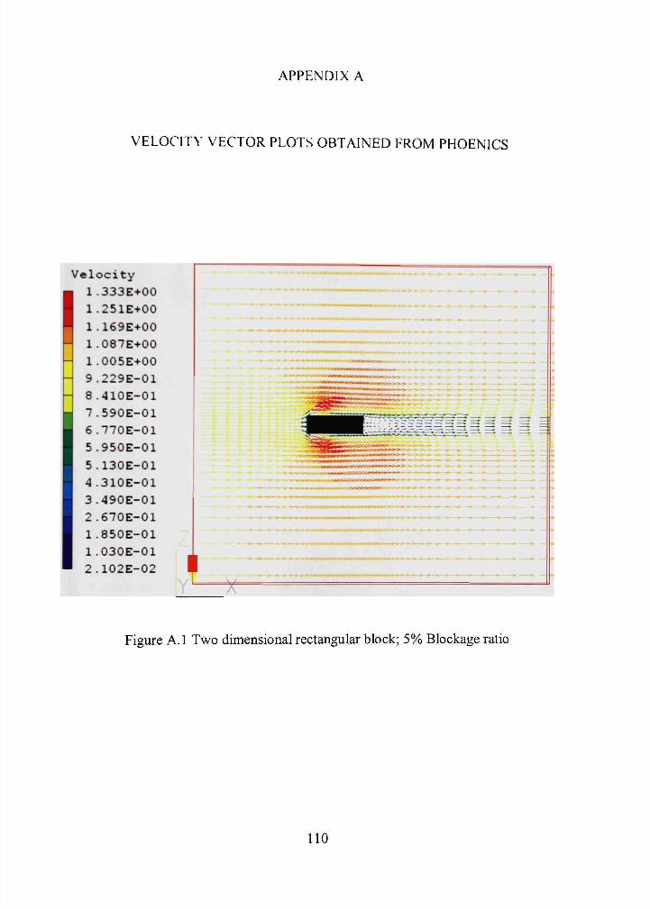
APPENDIX A
VELOCITY VECTOR PLOTS OBTAINED FROM PHOENICS
1 1 1 1 9
Velocity
I I .333E+00 1 .251E+00 1,169E+00 ,087E+00 ,005E+00 ,229E-01
8.410E-01 7.590E-01 6.770E-01 5.950E-01 5.130E-01 4.310E-01 3.490E-01 2.670E-01 1.850E-01 1.030E-01 2.102E-02
Figure A.l Two dimensional rectangular block; 5% Blockage ratio
110
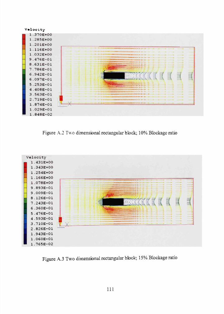
v e l o c i t y • 1.370E+00
1 1 .285E+00
1 1.201E>00 • 1 . 116E-t-00
- 1.032E+00
- 9.476E-01
- 8.631E-01
7 786E-01
6 ,942E-01
6 .097E-01
5 .253E-01
•1 ,408E-01
3 S63E-01
2,719E-01 1
1.874E-01 :'
1 029E-01
1 .848E-02
i • 4.;
™ .--
• * • * * * - — -
7^^.'.'.'....: '
'^fe^.;" ""^"" -—"- '"T-
^ -"*—' -
-- .,., » ,_. _ •'V — —
^ S 3 lill
llil
Figure .\.2 Two dimensional rectangular block; 10% Blockage ratio
Velocity
I I ,431E+00
1.343E+00
1.254E+00
1 .166E+00
1 .078E+00
9 .893E-01
9.009E-01
8.126E-01
7.243E-01
6 .360E-01
5 .476E-01
4 .593E-01
3 .710E-01
2.826E-01
1 .943E-01
1.060E-01
1 .765E-02
i X •'•.•».*"»g.»»a^
Figure A.3 Two dunensional rectangular block; 15% Blockage ratio
111
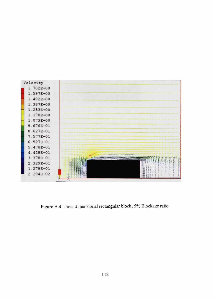
i 1
1
1
1
1
9
Velocity
I I.702E+00
1.597E+00
_ 1.492E+00
387E+00
283E+00
178E+00
073E+00
676E-01
8 .627E-01
7.577E-01
6.527E-01
5.478E-01
4.428E-01
3 .378E-01
2 .329E-01
1.279E-01
2.294E-02
Figure A.4 Three dimensional rectangular block; 5% Blockage ratio
112
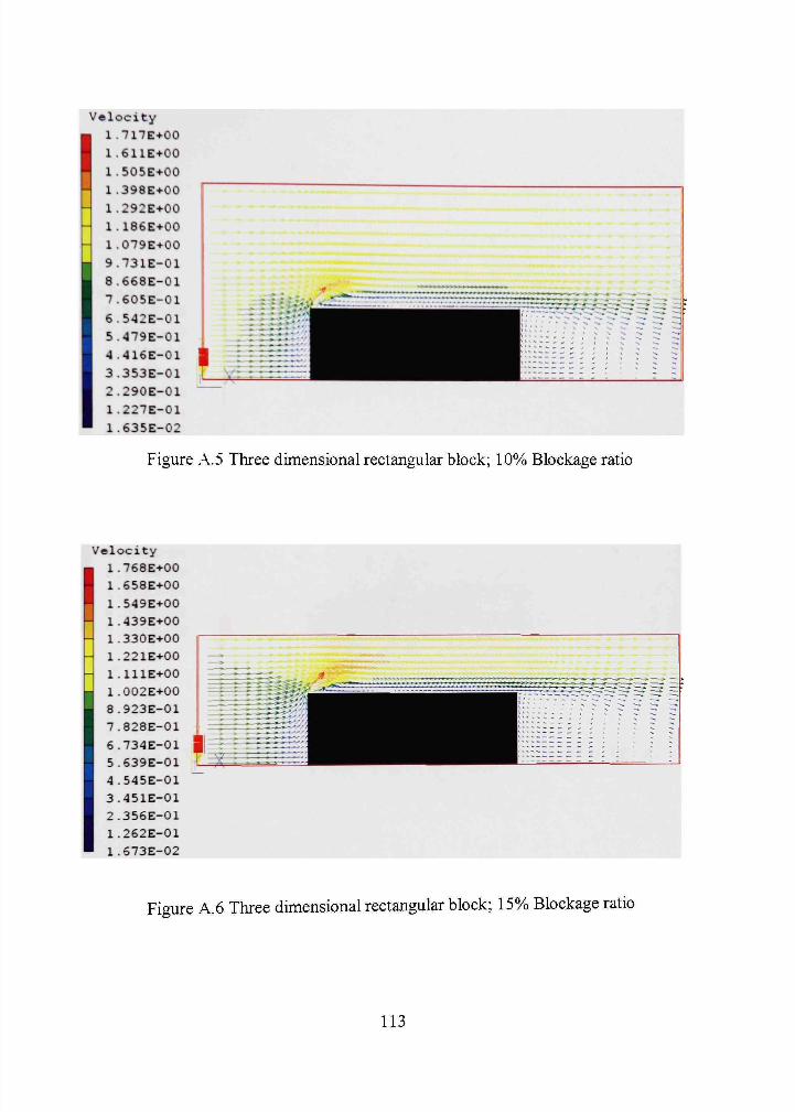
Velocity
I I.717E+00
1.611E+00
1.505E+00
1.398E+00
292E+00
186E+00
1.079E+00
9,731E-C1
,668E-01
,605E-01
542E-01
,479E-01
,416E-01
.353E-01
2.290E-01
1.227E-01
1 .635E-02
I X^
Figure .\.5 Three dimensional rectangular block; 10%) Blockage ratio
Velocity
I I.768E+00
1 .658E+00
1.549E+00
1.439E+00
1.330E+00
1.221E+00
1.lllE+00
1.002E+00
8.923E-01
7.828E-01
6.734E-01
5.639E-01
4.545E-01
3.451E-01
2.356E-01
1.262E-01
1.673E-02
Figure A.6 Three dimensional rectangular block; 15% Blockage ratio
113
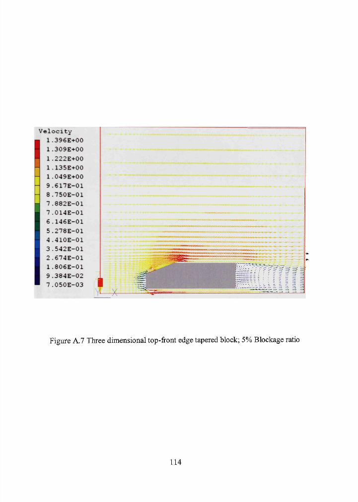
Velocity
I I .396E+00
1 .309E+00
1 .222E+00
1 .135E-t-00
1.049E+00
9.617E-01
8.750E-01
7.882E-01
7.014E-01
6.146E-01
5.278E-01
4.410E-01
3.542E-01
2.674E-01
1.806E-01
9.384E-02
7.050E-03
Figure A.7 Three dimensional top-front edge tapered block; 5% Blockage ratio
114
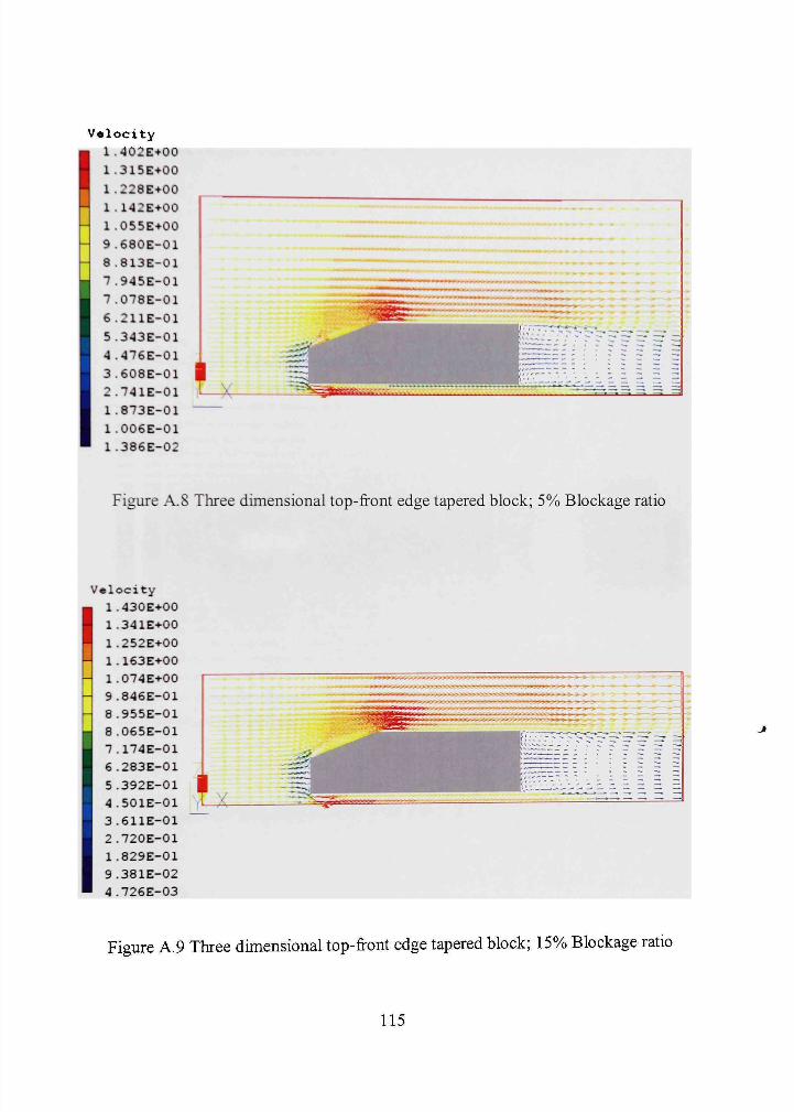
Vel
I 1 1 1 1 - 1
- 1
- 9
- 8
7
7
6
5
4
3
2
1
1
1
ocity
402E+00 315E+00
228E+00
142E+00
055E+00
680E-01
813E-01
945E-01
.078E-01
.211E-01
.343E-01
.476E-01
.608E-01
,741E-01
,873E-01
,006E-01
.386E-02
Figure A.S Three dimensional top-front edge tapered block; 5% Blockage ratio
I e l o c i t y 1.430E+00
1.341E+00
1.252E+00
1.163E+00
1.074E+00
9.846E-01
8.955E-01
8.065E-01
7.174E-01
6.283E-01
5.392E-01
4.501E-01
3.611E-01
2.720E-01
1.829E-01
9.381E-02
4.726E-03
—* * >--
Figure A.9 Three dimensional top-front edge tapered block; 15% Blockage ratio
115
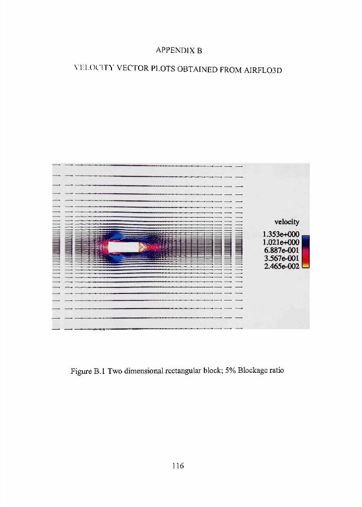
APPENDIX B
\ 1:1 OCITY VECTOR PLOTS OBTAINED FROM AIRFL03D
velocity
L353e+000 1.021e-f<X)0 6.887e-001 3.567e-001 2.465e-002 I
Figure B.l Two dimensional rectangular block; 5% Blockage ratio
116
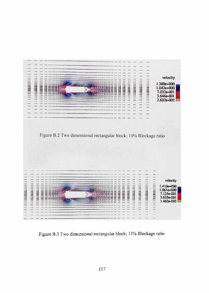
Figure B.2 Two dimensional rectangular block; 10% Blockage ratio
velocity
1.410e4O00 1.061e4<300 7.125e-001 3.635e-001 1.462e-002 I
Figure B.3 Two dimensional rectangular block; 15% Blockage ratio
117
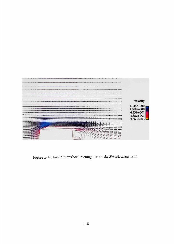
simil,.' J ' ^ 11 i i 3 s =i =? = ^^^M
velocity
1.344e+000 L009e+000 6.739e-001 3.387e-001 3.563e-003 !
Figure B.4 Three dimensional rectangular block; 5% Blockage ratio
118
velocity
1.352e-KK)0 1.016e4<K)0 6.799C-001 3.441e-001 8.242e-003 I
^^
Fiaure B.5 Three dimensional rectangular block; 10% Blockage ratio
velocity
1.399e+000 l.OSOe+OOO 7.017e-001 3J32e-001 4.657e-003 I
Figure B.6 Three dimensional rectangular block; 15% Blockage ratio
119
velodty
1.390e+O00 1.048e-K)00 7.069e-001 3.655e-001 2.408e-002 I
Figure B.7 Three dimensional top-front edge tapered block; 5% Blockage ratio
120
—• —• velocity
L406e-K)00 1.060e-K)00 7.147e-001 3.691e-001 2.351e-002 H
Figure B.S Three dimensional top-front edge tapered block; 10% Blockage ratio
—; —• velocity
1.459e+000 1.097e+000 7.3476-001 3.726e-001 ].046e-002 J
Figure B.9 Three dimensional top-front edge tapered block; 15% Blockage ratio
121
PERMISSION TO COPY
In presenting tbis tliesis in partial fulfillment of the requfrements for a master's
degree at Texas Tech Universit>' or Texas Tech University Health Sciences Center, I
agree that the Librar>- and m>' major department shall make it freely available for
research purposes. Permission to copy this thesis for scholarly purposes may be
granted b>' the Dfrector of the Library or my major professor. It is understood that any
copying or publication of this thesis for financial gain shall not be allowed without my
further wTitten permission and that any user may be liable for copyright infringement.
Agree (Permission is granted.)
Student-'jignaiure Date
Disagree (Permission is not granted.)
Student Signature Date