Window Dressing in Mutual Funds - Georgia State Universityfncvaa/Windowdressing RFS_FINAL.pdf · Wang,andChongXiaofortheirhelpfulcommentsandconstructivesuggestions ... (Carhart et

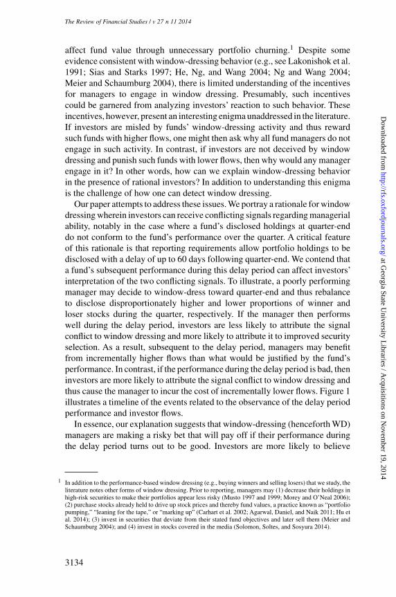
[18:05 9/10/2014 RFS-hhu045.tex] Page: 3133 3133–3170

Window Dressing in Mutual Funds

Vikas AgarwalRobinson College of Business, Georgia State University

Gerald D. GayRobinson College of Business, Georgia State University

Leng LingBunting College of Business, Georgia College & State University

We provide a rationale for window dressing wherein investors respond to conflicting signalsof managerial ability inferred from a fund’s performance and disclosed portfolio holdings.We contend that window dressers make a risky bet on their performance during a reportingdelay period, which affects investors’ interpretation of the conflicting signals and hencetheir capital allocations. Conditional on good (bad) performance, window dressers benefit(suffer) from higher (lower) investor flows compared with non–window dressers. Windowdressers also show poor past performance, possess little skill, and incur high portfolioturnover and trade costs, characteristics which in turn result in worse future performance.(JEL G11, G23)

An alleged agency problem in the mutual fund industry involves managersaltering or distorting their portfolios in an attempt to mislead investors abouttheir true ability by disclosing disproportionately higher (lower) holdings instocks that have done well (poorly) over a reporting period. This practice,commonly referred to as window dressing, has the potential to adversely

Vikas Agarwal acknowledges research support from the Centre for Financial Research (CFR) at the Universityof Cologne and from Georgia State University. Leng Ling acknowledges research grant support from GeorgiaCollege & State University. We thank Ranadeb Chaudhuri, Mark Chen, Conrad Ciccotello, Gjergji Cici, K. J.Martijn Cremers, Elroy Dimson, Jesse Ellis, Wayne Ferson, Jason Greene, Zhishan Guo, Zoran Ivkovic, MarcinKacperczyk, Jayant Kale, Aneel Keswani, Omesh Kini, Bing Liang, Reza Mahani, Ernst Maug, David Musto,Tiago Pinheiro, Chip Ryan, Thomas Schneeweis, Clemens Sialm, Vijay Singal, Tao Shu, Daniel Urban, QinghaiWang, and Chong Xiao for their helpful comments and constructive suggestions. We benefited from the commentsreceived at presentations at the Bank of Canada, Cass Business School, the Financial Intermediation ResearchSociety (FIRS) 2012 Conference, the Financial Management Association 2012 Conference, the Midwest FinanceAssociation 2013 Conference, the Southern FinanceAssociation 2012 Conference, the University ofAlabama, theUniversity of Cambridge, the University of Georgia, the University of Mannheim, the University of MassachusettsAmherst, and Wuhan University. We acknowledge the research assistance of Sujuan Ma, Jinfei Sheng, and HaibeiZhao and thank Linlin Ma and Yuehua Tang for sharing some of the data used in the empirical analysis. Weare grateful to Gang Hu, Paul Irvine, and Kumar Venkataraman for their help with the Abel Noser data andcomputation of trade costs. Finally, we wish to thank the editor (Laura Starks) and the referee for many valuablecomments and suggestions. Supplementary data can be found on The Review of Financial Studies web site. Sendcorrespondence to Leng Ling, Georgia College & State University (GCSU), Bunting College of Business, Suite414, Milledgeville, GA 31061; telephone: (478) 445-2587. E-mail: [email protected].

© The Author 2014. Published by Oxford University Press on behalf of The Society for Financial Studies.All rights reserved. For Permissions, please e-mail: [email protected]:10.1093/rfs/hhu045 Advance Access publication July 15, 2014

at Georgia State U

niversity Libraries / A

cquisitions on Novem

ber 19, 2014http://rfs.oxfordjournals.org/

Dow

nloaded from

http://rfs.oxfordjournals.org/

[18:05 9/10/2014 RFS-hhu045.tex] Page: 3134 3133–3170

The Review of Financial Studies / v 27 n 11 2014

affect fund value through unnecessary portfolio churning.1 Despite someevidence consistent with window-dressing behavior (e.g., see Lakonishok et al.1991; Sias and Starks 1997; He, Ng, and Wang 2004; Ng and Wang 2004;Meier and Schaumburg 2004), there is limited understanding of the incentivesfor managers to engage in window dressing. Presumably, such incentivescould be garnered from analyzing investors’ reaction to such behavior. Theseincentives, however, present an interesting enigma unaddressed in the literature.If investors are misled by funds’ window-dressing activity and thus rewardsuch funds with higher flows, one might then ask why all fund managers do notengage in such activity. In contrast, if investors are not deceived by windowdressing and punish such funds with lower flows, then why would any managerengage in it? In other words, how can we explain window-dressing behaviorin the presence of rational investors? In addition to understanding this enigmais the challenge of how one can detect window dressing.

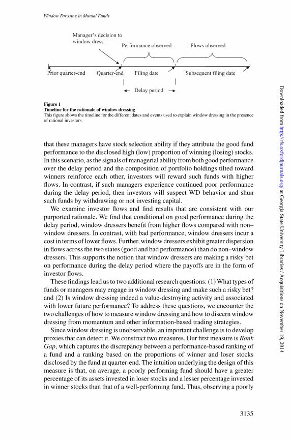
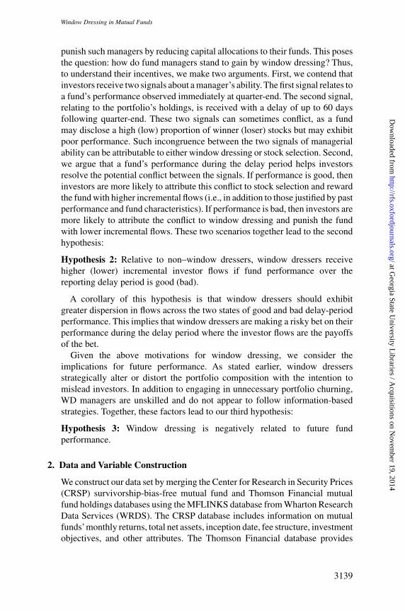
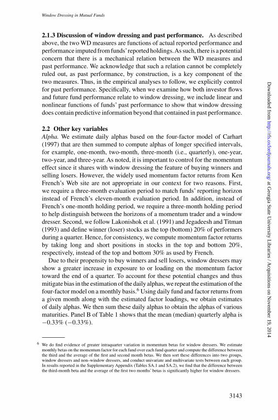
Our paper attempts to address these issues. We portray a rationale for windowdressing wherein investors can receive conflicting signals regarding managerialability, notably in the case where a fund’s disclosed holdings at quarter-enddo not conform to the fund’s performance over the quarter. A critical featureof this rationale is that reporting requirements allow portfolio holdings to bedisclosed with a delay of up to 60 days following quarter-end. We contend thata fund’s subsequent performance during this delay period can affect investors’interpretation of the two conflicting signals. To illustrate, a poorly performingmanager may decide to window-dress toward quarter-end and thus rebalanceto disclose disproportionately higher and lower proportions of winner andloser stocks during the quarter, respectively. If the manager then performswell during the delay period, investors are less likely to attribute the signalconflict to window dressing and more likely to attribute it to improved securityselection. As a result, subsequent to the delay period, managers may benefitfrom incrementally higher flows than what would be justified by the fund’sperformance. In contrast, if the performance during the delay period is bad, theninvestors are more likely to attribute the signal conflict to window dressing andthus cause the manager to incur the cost of incrementally lower flows. Figure 1illustrates a timeline of the events related to the observance of the delay periodperformance and investor flows.

In essence, our explanation suggests that window-dressing (henceforth WD)managers are making a risky bet that will pay off if their performance duringthe delay period turns out to be good. Investors are more likely to believe

1 In addition to the performance-based window dressing (e.g., buying winners and selling losers) that we study, theliterature notes other forms of window dressing. Prior to reporting, managers may (1) decrease their holdings inhigh-risk securities to make their portfolios appear less risky (Musto 1997 and 1999; Morey and O’Neal 2006);(2) purchase stocks already held to drive up stock prices and thereby fund values, a practice known as “portfoliopumping,” “leaning for the tape,” or “marking up” (Carhart et al. 2002; Agarwal, Daniel, and Naik 2011; Hu etal. 2014); (3) invest in securities that deviate from their stated fund objectives and later sell them (Meier andSchaumburg 2004); and (4) invest in stocks covered in the media (Solomon, Soltes, and Sosyura 2014).

3134

at Georgia State U




Dow

nloaded from


[18:05 9/10/2014 RFS-hhu045.tex] Page: 3135 3133–3170


Prior quarter-end Quarter-end Filing date Subsequent filing date

Performance observed

Manager’s decision to window dress

Flows observed

Delay period

Figure 1Timeline for the rationale of window dressingThis figure shows the timeline for the different dates and events used to explain window dressing in the presenceof rational investors.

that these managers have stock selection ability if they attribute the good fundperformance to the disclosed high (low) proportion of winning (losing) stocks.In this scenario, as the signals of managerial ability from both good performanceover the delay period and the composition of portfolio holdings tilted towardwinners reinforce each other, investors will reward such funds with higherflows. In contrast, if such managers experience continued poor performanceduring the delay period, then investors will suspect WD behavior and shunsuch funds by withdrawing or not investing capital.

We examine investor flows and find results that are consistent with ourpurported rationale. We find that conditional on good performance during thedelay period, window dressers benefit from higher flows compared with non–window dressers. In contrast, with bad performance, window dressers incur acost in terms of lower flows. Further, window dressers exhibit greater dispersionin flows across the two states (good and bad performance) than do non–windowdressers. This supports the notion that window dressers are making a risky beton performance during the delay period where the payoffs are in the form ofinvestor flows.

These findings lead us to two additional research questions: (1) What types offunds or managers may engage in window dressing and make such a risky bet?and (2) Is window dressing indeed a value-destroying activity and associatedwith lower future performance? To address these questions, we encounter thetwo challenges of how to measure window dressing and how to discern windowdressing from momentum and other information-based trading strategies.

Since window dressing is unobservable, an important challenge is to developproxies that can detect it. We construct two measures. Our first measure is RankGap, which captures the discrepancy between a performance-based ranking ofa fund and a ranking based on the proportions of winner and loser stocksdisclosed by the fund at quarter-end. The intuition underlying the design of thismeasure is that, on average, a poorly performing fund should have a greaterpercentage of its assets invested in loser stocks and a lesser percentage investedin winner stocks than that of a well-performing fund. Thus, observing a poorly

3135

at Georgia State U




Dow

nloaded from


[18:05 9/10/2014 RFS-hhu045.tex] Page: 3136 3133–3170


performing fund with a high percentage of disclosed holdings in winners anda low percentage in losers would suggest a greater likelihood of WD behavior.Since Rank Gap is based on ranking a fund’s performance as well as its winnerand loser proportions relative to other funds, it can be viewed as a relativemeasure.

Our second measure is Backward Holding Return Gap (BHRG), an absolutemeasure that compares the hypothetical return of a fund’s reported holdings withthe fund’s actual return. This measure is motivated by the work of Kacperczyk,Sialm, and Zheng (2008) (henceforth KSZ), who compare a fund’s actualperformance with the performance of the fund’s prior quarter-end portfolio,assuming it to be held throughout the current quarter. They refer to the differencebetween the two returns as “return gap” and attribute it to manager skill. Sincewe are studying WD behavior, we use instead the current quarter-end portfolioand assume that a manager held it from the beginning of the current quarter. Theintuition is that a WD manager upon observing winner and loser stocks towardthe quarter-end will tilt portfolio holdings toward winner stocks and away fromloser stocks to give investors a false impression of stock selection ability. Wethus compute BHRG as the difference between (a) the return imputed fromthe reported quarter-end portfolio (assuming that the manager held this sameportfolio at the beginning of the quarter) after adjusting for trade costs andexpenses; and (b) the fund’s actual quarterly return.2

Using our measures, we investigate (a) the characteristics of funds andmanagers that engage in window dressing, and (b) the effects of windowdressing on future performance. We find that WD behavior is associated withmanagers having poor performance and lacking skill, which perhaps justifieswhy certain managers choose to engage in the risky bet associated withwindow dressing. Interestingly, this finding resonates well with the literaturedocumenting a positive association between career concerns of managers andtheir risk-taking behavior (see Khorana 1996; Brown, Harlow, and Starks1996; Chevalier and Ellison 1997). We also find that WD managers engagein excessive turnover of stocks in both their WD-related and other trading.Using Abel Noser institutional transaction data, we show that window dressingresults in significantly higher levels of trade costs. Further, separating windowdressers’ trade costs into explicit and implicit components, we find the implicitcomponent to be particularly higher, consistent with window dressers havingan urgency to trade (buy winners and sell losers) near quarter-ends.

Given that WD managers appear to be unskilled, follow non-information-based trading strategies, and incur high levels of trade costs, we conjecturethat their future performance should be poor on average. Controlling for

2 To help demonstrate the distinction between our BHRG measure and KSZ’s return gap measure, we provide anumerical illustration in the Supplementary Appendix (available on the RFS Web site) that shows how BHRGhelps identify a WD manager while the return gap measure helps identify a skilled manager.

3136

at Georgia State U




Dow

nloaded from

http://rfs.oxfordjournals.org/lookup/suppl/doi:10.1093/rfs/hhu045/-/DC1


[18:05 9/10/2014 RFS-hhu045.tex] Page: 3137 3133–3170


past performance, we find that both short-term and long-term future fundperformance is negatively related to window dressing.

Our findings that window dressing is associated with poor past performanceas well as lower future performance show that the BHRG and Rank Gapmeasures are capturing window dressing rather than momentum trading. Tohelp further make this distinction, we conduct two seasonality tests. We firstexamine the intraquarter variation in a fund’s exposure to recent winners withthe intuition that the exposure for momentum traders should be uniformlydistributed due to the monthly rebalancing or updating of winners inherent inthe strategy. In contrast, for window dressers the exposure should increase in thethird month of the quarter due to the purchase of winners toward quarter-end.In the second test, we examine the intraquarter variation in WD behavior forDecember versus other fiscal quarter month-ends. There are two reasons for thistest. First, the literature on tournaments and the flow-performance relation (e.g.,Brown, Harlow, and Starks 1996; Chevalier and Ellison 1997; Sirri and Tufano1998; Huang, Wei, and Yan 2007) suggests that many investors evaluate fundson a calendar-year basis, which may provide greater incentives to window-dressin December. Second, window dressers may disguise their behavior by sellinglosing stocks in December and thus pooling themselves with tax-loss sellers.Therefore, window dressing should be more pronounced in December whilemomentum trading should be more uniformly distributed over the year. Thefindings from these tests further corroborate that our measures are capturingwindow dressing and not momentum trading.

Our paper also builds on a broader literature that studies the effects ofportfolio disclosure on the investment decisions of money managers (Musto1997, 1999); the consequences of portfolio disclosure, such as free riding andfront-running (Wermers 2001; Frank et al. 2004; Brown and Schwarz 2011;Verbeek and Wang 2013); the determinants of portfolio disclosure and itseffect on performance and flows (Ge and Zheng 2006); the motivation behindinstitutions seeking confidentiality for their 13F filings (Aragon, Hertzel, andShi 2013; Agarwal et al. 2013); and the effect of mandatory portfolio disclosureon stock liquidity and on the performance of disclosing mutual funds (Agarwalet al. Forthcoming).

1. Related Literature and Testable Hypotheses

1.1 Related literatureOne strand of related literature studies the relation between the turn-of-the-yeareffect and window dressing by institutional investors. Haugen and Lakonishok(1988) and Ritter and Chopra (1989) argue that window dressing can potentiallyexplain the January effect. Sias and Starks (1997), Poterba and Weisbenner(2001), and Chen and Singal (2004) attempt to disentangle tax-loss sellingand WD explanations for the turn-of-the-year effect and provide evidence insupport of tax-loss selling. Starks, Yong, and Zheng (2006) sharpen tests in

3137

at Georgia State U




Dow

nloaded from


[18:05 9/10/2014 RFS-hhu045.tex] Page: 3138 3133–3170


these prior studies by studying municipal bond closed-end funds to providefurther support for tax-loss selling driving the January effect.

Another strand of literature studies the trading behavior of institutions aroundquarter-ends to find evidence suggestive of window dressing. Lakonishok et al.(1991) examine the quarterly equity holdings of pension funds and showthat they sell more losers in the fourth quarter of the year. Similarly, He,Ng, and Wang (2004) show that institutions who invest on behalf of clientssell more poorly performing stocks during the fourth quarter. Moreover, thistrading behavior is more pronounced for institutions whose portfolios haveunderperformed. Ng and Wang (2004) find that institutions sell more extremelosing small stocks in the fourth quarter. Meier and Schaumburg (2004) proposeshape tests for alternative trading patterns and find evidence consistent withwindow dressing in equity mutual funds.

Finally, in a more recent study, G. Hu et al. (2014) analyze the equitytransactions of institutions (e.g., mutual fund families and plan sponsors) thatreport to Abel Noser. Although their main focus is on portfolio pumping, theyalso study the practice of buying winners and selling losers at calendar quarter-ends and conclude that window dressing is not a widespread phenomenon.While their finding may at first appear contrary to ours, it is important to notethat we contend that only some funds appear to engage in WD behavior. Further,there are several factors that can help reconcile the findings of the two studies.First, our analysis is at the individual fund level rather than at the mutual fundfamily level, and excludes index funds and nonequity funds. Moreover, ourempirical design enables us to shed light on specific fund characteristics thatprovide incentives to window-dress. Second, we believe that it is difficult toascertain window dressing from institutional trade data. Thus, we use a fund’sdisclosed portfolio holdings and performance to develop direct measures of thepropensity to window-dress. Third, we examine funds’ WD behavior at fiscalquarter-ends to coincide with the timing of funds’ portfolio disclosures insteadof using calendar quarter-ends as in G. Hu et al. (2014).

1.2 HypothesesWe posit that managers having low skill and achieving poor performance earlierduring a quarter (e.g., during the first two months) are more likely to window-dress. The rationale is that these managers choose to window-dress as a lastresort when they have performed poorly and/or have limited skill, and thereforehave little expectation that they will perform better in the future. This leads toour first hypothesis:

Hypothesis 1: Window dressing is negatively related to fund performanceduring the first two months of a quarter and to manager skill.

A critical issue missing from the literature relates to the incentives ofmanagers to engage in window dressing. If investors believe managers misleadby strategically changing their portfolios prior to quarter-ends, investors should

3138

at Georgia State U




Dow

nloaded from


[18:05 9/10/2014 RFS-hhu045.tex] Page: 3139 3133–3170


punish such managers by reducing capital allocations to their funds. This posesthe question: how do fund managers stand to gain by window dressing? Thus,to understand their incentives, we make two arguments. First, we contend thatinvestors receive two signals about a manager’s ability. The first signal relates toa fund’s performance observed immediately at quarter-end. The second signal,relating to the portfolio’s holdings, is received with a delay of up to 60 daysfollowing quarter-end. These two signals can sometimes conflict, as a fundmay disclose a high (low) proportion of winner (loser) stocks but may exhibitpoor performance. Such incongruence between the two signals of managerialability can be attributable to either window dressing or stock selection. Second,we argue that a fund’s performance during the delay period helps investorsresolve the potential conflict between the signals. If performance is good, theninvestors are more likely to attribute this conflict to stock selection and rewardthe fund with higher incremental flows (i.e., in addition to those justified by pastperformance and fund characteristics). If performance is bad, then investors aremore likely to attribute the conflict to window dressing and punish the fundwith lower incremental flows. These two scenarios together lead to the secondhypothesis:

Hypothesis 2: Relative to non–window dressers, window dressers receivehigher (lower) incremental investor flows if fund performance over thereporting delay period is good (bad).

A corollary of this hypothesis is that window dressers should exhibitgreater dispersion in flows across the two states of good and bad delay-periodperformance. This implies that window dressers are making a risky bet on theirperformance during the delay period where the investor flows are the payoffsof the bet.

Given the above motivations for window dressing, we consider theimplications for future performance. As stated earlier, window dressersstrategically alter or distort the portfolio composition with the intention tomislead investors. In addition to engaging in unnecessary portfolio churning,WD managers are unskilled and do not appear to follow information-basedstrategies. Together, these factors lead to our third hypothesis:

Hypothesis 3: Window dressing is negatively related to future fundperformance.

2. Data and Variable Construction

We construct our data set by merging the Center for Research in Security Prices(CRSP) survivorship-bias-free mutual fund and Thomson Financial mutualfund holdings databases using the MFLINKS database from Wharton ResearchData Services (WRDS). The CRSP database includes information on mutualfunds’monthly returns, total net assets, inception date, fee structure, investmentobjectives, and other attributes. The Thomson Financial database provides

3139

at Georgia State U




Dow

nloaded from


[18:05 9/10/2014 RFS-hhu045.tex] Page: 3140 3133–3170


quarterly or semiannual holdings of mutual funds in our sample.3 As our focus ison U.S. equity funds, we exclude balanced, bond, international, money market,and sector funds. Since the CRSP database provides information at the share-class level, we aggregate data at the fund level by weighting each share classby its total net assets to obtain value-weighted averages of monthly returns andannual expense ratios. Our final sample comprises 59,060 quarterly reportsfrom 2,623 equity funds that span the period September 1998 to December2008.4

2.1 Measures of window dressingWe develop two measures of window dressing that are based on reported fundholdings and returns. More specifically, we propose both a relative and anabsolute measure that capture the inconsistency between a fund’s reportedperformance based on net asset values and performance imputed from itsdisclosed holdings.

2.1.1 Rank Gap Relative measure of window dressing. At the end of eachfund’s fiscal quarter, we create quintiles of all domestic stocks in the CRSPstockdatabase by sorting stocks in descending order according to their returns overthe past three months. The first (fifth) quintile consists of stocks that achievethe highest (lowest) returns. Then, using each fund’s reported holdings, weidentify stocks that belong to different quintiles and calculate the proportionsof the fund’s assets invested in the first and fifth quintiles. In the spirit ofLakonishok et al. (1991) and Jegadeesh and Titman (1993), we refer to thesetwo extreme quintiles as winner and loser proportions, respectively.

Next, for each fiscal quarter that has at least 100 funds reporting holdings, werank the funds in three ways. For the first ranking, we sort funds in descendingorder by their quarterly returns, with funds in the 1st percentile bin being thebest performing funds (and all assigned a rank equal to 1) and funds in the100th percentile bin being the worst (and assigned a rank equal to 100). For thesecond ranking, we sort funds in descending order according to their proportionof winner stock holdings and again assign ranks between 1 and 100, with fundsin the 1st (100th) percentile bin having the highest (lowest) winner proportion.For the third ranking, we sort funds in ascending order according to theirproportion of loser stock holdings and assign ranks similarly. Hence, funds in

3 Under the Securities Act of 1933, the Securities Exchange Act of 1934, and the Investment CompanyAct of 1940, mutual fund managers are required to periodically disclose their holdings. Following a 1985amendment, funds were required to submit annual and semiannual reports (N-CSR and N-CSRS, respectively);however, a large majority of managers voluntarily continued to disclose portfolio holdings on a quarterlybasis as was previously required. Effective May 10, 2004, the SEC requires investment companies todisclose as of the end of the first and the third fiscal quarters as well, on Form N-Q. For further detail, seehttp://www.sec.gov/rules/final/33-8393.htm#IB.

4 Although mutual fund holdings data are available since January 1980, our sample period starts in September1998, corresponding to when daily fund return data became available to estimate daily four-factor alphas.

3140

at Georgia State U




Dow

nloaded from

http://www.sec.gov/rules/final/33-8393.htm#IB


[18:05 9/10/2014 RFS-hhu045.tex] Page: 3141 3133–3170


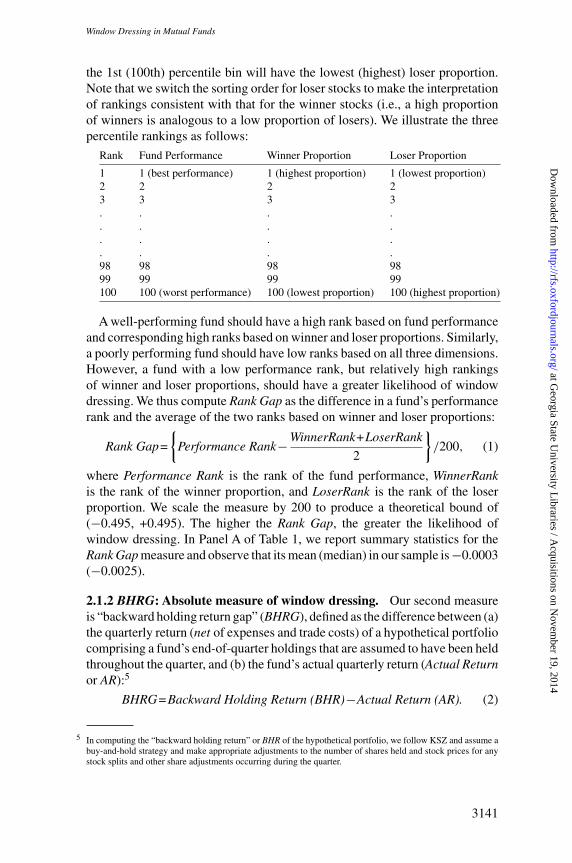
the 1st (100th) percentile bin will have the lowest (highest) loser proportion.Note that we switch the sorting order for loser stocks to make the interpretationof rankings consistent with that for the winner stocks (i.e., a high proportionof winners is analogous to a low proportion of losers). We illustrate the threepercentile rankings as follows:

Rank Fund Performance Winner Proportion Loser Proportion

1 1 (best performance) 1 (highest proportion) 1 (lowest proportion)2 2 2 23 3 3 3. . . .. . . .. . . .. . . .98 98 98 9899 99 99 99100 100 (worst performance) 100 (lowest proportion) 100 (highest proportion)

A well-performing fund should have a high rank based on fund performanceand corresponding high ranks based on winner and loser proportions. Similarly,a poorly performing fund should have low ranks based on all three dimensions.However, a fund with a low performance rank, but relatively high rankingsof winner and loser proportions, should have a greater likelihood of windowdressing. We thus compute Rank Gap as the difference in a fund’s performancerank and the average of the two ranks based on winner and loser proportions:

Rank Gap=

Performance Rank− WinnerRank+LoserRank

2

/200, (1)

where Performance Rank is the rank of the fund performance, WinnerRankis the rank of the winner proportion, and LoserRank is the rank of the loserproportion. We scale the measure by 200 to produce a theoretical bound of(−0.495, +0.495). The higher the Rank Gap, the greater the likelihood ofwindow dressing. In Panel A of Table 1, we report summary statistics for theRank Gap measure and observe that its mean (median) in our sample is −0.0003(−0.0025).

2.1.2 BHRG: Absolute measure of window dressing. Our second measureis “backward holding return gap” (BHRG), defined as the difference between (a)the quarterly return (net of expenses and trade costs) of a hypothetical portfoliocomprising a fund’s end-of-quarter holdings that are assumed to have been heldthroughout the quarter, and (b) the fund’s actual quarterly return (Actual Returnor AR):5

BHRG=Backward Holding Return (BHR)−Actual Return (AR). (2)

5 In computing the “backward holding return” or BHR of the hypothetical portfolio, we follow KSZ and assume abuy-and-hold strategy and make appropriate adjustments to the number of shares held and stock prices for anystock splits and other share adjustments occurring during the quarter.

3141

at Georgia State U




Dow

nloaded from


[18:05 9/10/2014 RFS-hhu045.tex] Page: 3142 3133–3170


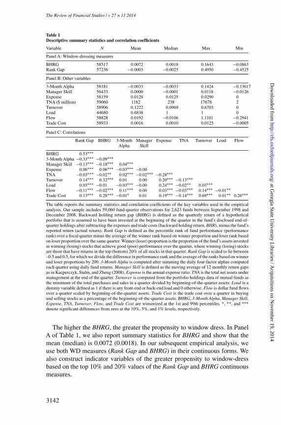
Table 1Descriptive summary statistics and correlation coefficients

Variable N Mean Median Max Min

Panel A: Window-dressing measures

BHRG 58517 0.0072 0.0018 0.1643 −0.0863Rank Gap 57236 −0.0003 −0.0025 0.4950 −0.4525

Panel B: Other variables

3-Month Alpha 58181 −0.0033 −0.0033 0.1424 −0.13617Manager Skill 56433 0.0000 −0.0001 0.0118 −0.0126Expense 58159 0.0128 0.0125 0.0290 0TNA ($ million) 59060 1182 238 17678 2Turnover 58906 0.1222 0.0969 0.6703 0Load 44680 0.6838 1 1 0Flow 58828 0.0192 −0.0106 1.1101 −0.2941Trade Cost 58933 0.0016 0.0010 0.0125 −0.0005

Panel C: Correlations

Rank Gap BHRG 3-Month Manager Expense TNA Turnover Load FlowAlpha Skill

BHRG 0.53∗∗∗3-Month Alpha −0.33∗∗∗ −0.09∗∗∗Manager Skill −0.13∗∗∗ −0.18∗∗∗ 0.04∗∗∗Expense 0.06∗∗∗ 0.06∗∗∗ −0.03∗∗∗ −0.00TNA −0.03∗∗∗ −0.02∗∗ 0.02∗∗∗ −0.02∗∗∗ −0.28∗∗∗Turnover 0.14∗∗∗ 0.32∗∗∗ 0.01 0.00 0.20∗∗∗ −0.13∗∗∗Load 0.03∗∗∗ −0.01 −0.03∗∗∗ −0.00 0.24∗∗∗ −0.02∗∗ 0.03∗∗∗Flow −0.11∗∗∗ −0.02∗∗∗ 0.11∗∗∗ 0.00 0.03∗∗∗ −0.03∗∗∗ 0.14∗∗∗ −0.01∗∗Trade Cost 0.13∗∗∗ 0.28∗∗∗ −0.01∗ 0.01 0.19∗∗∗ −0.14∗∗∗ 0.69∗∗∗ 0.01∗∗ 0.26∗∗∗

The table reports the summary statistics and correlation coefficients of the key variables used in the empiricalanalysis. Our sample includes 59,060 fund-quarter observations for 2,623 funds between September 1998 andDecember 2008. Backward holding return gap (BHRG) is defined as the quarterly return of a hypotheticalportfolio that is assumed to have been invested at the beginning of the quarter in the fund’s disclosed end-of-quarter holdings after subtracting the expenses and trade costs (backward holding return, BHR), minus the fund’sreported return (actual return). Rank Gap is defined as the percentile rank of fund performance (performancerank) over a fiscal quarter minus the average of the winner rank based on winner proportion and loser rank basedon loser proportion over the same quarter. Winner (loser) proportion is the proportion of the fund’s assets investedin winning (losing) stocks that achieve good (poor) performance over the quarter, where winning (losing) stocksare those that have returns in the top (bottom) 20% of all stocks in that quarter. Rank Gap is scaled to lie between–0.5 and 0.5, for which we divide the difference in performance rank and the average of the ranks based on winnerand loser proportions by 200. 3-Month Alpha is computed after summing the daily four-factor alphas computedeach quarter using daily fund returns. Manager Skill is defined as the moving average of 12 monthly return gapsas in Kacperczyk, Sialm, and Zheng (2008). Expense is the annual expense ratio. TNA is the total net assets undermanagement at the end of the quarter. Turnover is computed from the portfolio holdings data of mutual funds asthe minimum of the total purchases and sales in a quarter divided by beginning-of-the-quarter assets. Load is adummy variable defined as 1 if there is any front-end or back-end load and 0 otherwise. Flow is dollar fund flowsover a quarter scaled by beginning-of-the-quarter assets. Trade Cost is the trade cost over a quarter in buyingand selling stocks as a percentage of the beginning-of-the-quarter assets. BHRG, 3-Month Alpha, Manager Skill,Expense, TNA, Turnover, Flow, and Trade Cost are winsorized at the 1st and 99th percentiles. *, **, and ***denote significant differences from zero at the 10%, 5%, and 1% levels, respectively.

The higher the BHRG, the greater the propensity to window dress. In PanelA of Table 1, we also report summary statistics for BHRG and show that themean (median) is 0.0072 (0.0018). In our subsequent empirical analysis, weuse both WD measures (Rank Gap and BHRG) in their continuous forms. Wealso construct indicator variables of the greater propensity to window-dressbased on the top 10% and 20% values of the Rank Gap and BHRG continuousmeasures.

3142

at Georgia State U




Dow

nloaded from


[18:05 9/10/2014 RFS-hhu045.tex] Page: 3143 3133–3170


2.1.3 Discussion of window dressing and past performance. As describedabove, the two WD measures are functions of actual reported performance andperformance imputed from funds’reported holdings.As such, there is a potentialconcern that there is a mechanical relation between the WD measures andpast performance. We acknowledge that such a relation cannot be completelyruled out, as past performance, by construction, is a key component of thetwo measures. Thus, in the empirical analyses to follow, we explicitly controlfor past performance. Specifically, when we examine how both investor flowsand future fund performance relate to window dressing, we include linear andnonlinear functions of funds’ past performance to show that window dressingdoes contain predictive information beyond that contained in past performance.

2.2 Other key variablesAlpha. We estimate daily alphas based on the four-factor model of Carhart(1997) that are then summed to compute alphas of longer specified intervals,for example, one-month, two-month, three-month (i.e., quarterly), one-year,two-year, and three-year. As noted, it is important to control for the momentumeffect since it shares with window dressing the feature of buying winners andselling losers. However, the widely used momentum factor returns from KenFrench’s Web site are not appropriate in our context for two reasons. First,we require a three-month evaluation period to match funds’ reporting horizoninstead of French’s eleven-month evaluation period. In addition, instead ofFrench’s one-month holding period, we require a three-month holding periodto help distinguish between the horizons of a momentum trader and a windowdresser. Second, we follow Lakonishok et al. (1991) and Jegadeesh and Titman(1993) and define winner (loser) stocks as the top (bottom) 20% of performersduring a quarter. Hence, for consistency, we compute momentum factor returnsby taking long and short positions in stocks in the top and bottom 20%,respectively, instead of the top and bottom 30% as used by French.

Due to their propensity to buy winners and sell losers, window dressers mayshow a greater increase in exposure to or loading on the momentum factortoward the end of a quarter. To account for these potential changes and thusmitigate bias in the estimation of the daily alphas, we repeat the estimation of thefour-factor model on a monthly basis.6 Using daily fund and factor returns froma given month along with the estimated factor loadings, we obtain estimatesof daily alphas. We then sum these daily alphas to obtain the alphas of variousmaturities. Panel B of Table 1 shows that the mean (median) quarterly alpha is−0.33% (−0.33%).

6 We do find evidence of greater intraquarter variation in momentum betas for window dressers. We estimatemonthly betas on the momentum factor for each fund over each fund quarter and compute the difference betweenthe third and the average of the first and second month betas. We then sort these differences into two groups,window dressers and non–window dressers, and conduct univariate and multivariate tests between each group.In results reported in the Supplementary Appendix (Tables SA.1 and SA.2), we find that the difference betweenthe third-month beta and the average of the first two months’ betas is significantly higher for window dressers.

3143

at Georgia State U




Dow

nloaded from



[18:05 9/10/2014 RFS-hhu045.tex] Page: 3144 3133–3170


Flow. We calculate monthly net fund flows as[TNAt −TNAt−1 ·(1+rt )]/TNAt−1, where TNAt and TNAt−1 are the fund’s totalnet assets under management at the end of months t and t−1, respectively, andrt is the net-of-fee return during month t . Quarterly fund flows are computedby summing the dollar flows over the three months of the quarter and dividingby the total net assets at the beginning of the quarter. In Panel B of Table 1, weobserve that the mean (median) quarterly flow is 1.92% (−1.06%).

Trade Cost. We obtain information for computing trade costs from dailyinstitutional trades reported in the Abel Noser database during our sampleperiod. To compute a fund’s trade costs in a given fund quarter, we identify thefund’s buys and sells of each stock traded during the quarter by comparing itsbeginning and ending holdings. Then, for each stock bought or sold, we identifyin the Abel Noser database all institutions’ buys and sells of that stock duringthe same quarter.7 For each trade (keeping buys and sells separate) we computethe explicit trade cost per share by dividing the reported trade commission bythe number of shares in the transaction. We compute the implicit trade cost pershare for buys (sells) as the difference between the reported trade price (openprice) and the stock’s opening price (trade price) that day. The total trade costper share is computed as the sum of the explicit and implicit trade costs. Then,for all trades of the stock during the quarter, we compute separately for buysand sells the volume-weighted explicit, implicit, and total (unit) trade cost pershare. We repeat these calculations for each stock traded by the fund in thequarter.

We next link these unit trade costs to a fund’s buys and sells during thequarter and compute, for each trade, the explicit, implicit, and total trade costsby multiplying the unit trade costs by the trade size. We then sum the trade costsfor all trades by the fund during the quarter to obtain the total dollar trade costs,which we scale by the fund’s beginning-of-quarter TNA. We report in Panel Bof Table 1 that the mean (median) quarterly trade cost is 0.16% (0.10%).

Turnover. We compute a fund’s quarterly turnover ratio as the minimumof the dollar values of purchases and sales, divided by total net assets at thebeginning of the quarter. In Panel B of Table 1, we report the mean (median)quarterly portfolio turnover to be 12.2% (9.7%).

Manager Skill. For manager skill, we follow KSZ and use the 12-monthmoving average of the monthly return gap, which they show is positively relatedto future performance. In Panel B of Table 1, we report that the mean and medianmanager skill are both close to zero.

Style. We use the investment objective code (IOC) field from the ThomsonFinancial mutual fund holdings database to construct style dummies. Weexclude the four nonequity styles (international, municipal bonds, balanced,

7 We note that individual institutions are not identified in the Abel Noser database. Hence, we compute trade costsfor each stock based on the trades of all institutions during a given quarter of that stock.

3144

at Georgia State U




Dow

nloaded from


[18:05 9/10/2014 RFS-hhu045.tex] Page: 3145 3133–3170


and bonds & preferreds) and focus on the five active equity styles: aggressivegrowth, growth, growth & income, metals, and unclassified.8

Other variables used in the analysis include Size, defined as the log of a fund’sTNA; Expense, defined as a fund’s annual expense ratio; and Load, defined asan indicator variable having a value of 1 if a fund has a front-end or back-endload, and 0 otherwise.

2.3 CorrelationsPanel C of Table 1 provides the correlations between the key variables. Thetwo WD measures, Rank Gap and BHRG, have a strong positive correlation of0.53. In addition, we observe a negative correlation between both measures andquarterly alpha (−0.33 with Rank Gap, and −0.09 with BHRG). Further, thetwo measures are negatively correlated with manager skill (−0.13 and −0.18,respectively). Although these correlations are based on contemporaneousvalues and therefore do not necessarily imply causality, it is interesting thatthe signs of the correlations are consistent with our first hypothesis suggestingthat WD behavior is negatively related to past performance and manager skill.We also find that the WD measures are positively related to trade costs, expenseratio, and turnover, and negatively related to flows.

3. Window Dressing: Motivation and Attributes

3.1 Do investors respond to portfolio characteristics?In addition to information contained in past performance, there is growingevidence in the academic literature that investors use information based ondisclosed portfolio holdings to assess managerial ability.9 This evidence doesnot necessarily imply irrationality, since rational investors can use holdingsinformation as an ex ante measure of managerial ability in conjunction withpast performance, which is an ex post measure. If this is indeed the case theninvestor flows should respond to portfolio characteristics after controlling forpast performance. In the context of our study, these characteristics relate to theproportions of winners and losers in the disclosed portfolios. We examine therelation between fund flows and proportions of winners and losers, controllingfor past performance and other fund characteristics, and estimate the following

8 If a fund’s IOC is unclassified, we use the Lipper objective codes (EIEI, G, LCCE, LCGE, LCVE, MCCE,MCGE, MCVE, MLCE, MLGE, MLVE, SCCE, SCGE, SCVE), the Strategic Insight objective codes (AGG,GMC, GRI, GRO, ING, SCG), and Wiesenberger Fund Type codes (G, G-I, AGG, GCI, GRI, GRO, LTG, MCG,SCG) to identify whether the fund is an actively managed equity fund for inclusion in our sample.

9 See, for example, Grinblatt and Titman (1989, 1993); Grinblatt, Titman, and Wermers (1995); Daniel et al. (1997);Wermers (1999, 2000); Chen, Jegadeesh, and Wermers (2000); Gompers and Metrick (2001); Cohen, Coval, andPastor (2005); Kacperczyk, Sialm, and Zheng (2005, 2008); Sias, Starks, and Titman (2006); Alexander, Cici,and Gibson (2007); Jiang, Yao, and Yu (2007); Kacperczyk and Seru (2007); Cremers and Petajisto (2009); Bakeret al. (2010); Huang and Kale (2013).

3145

at Georgia State U




Dow

nloaded from


[18:05 9/10/2014 RFS-hhu045.tex] Page: 3146 3133–3170


regression:

Flowsi,t+1 =β0 +β1Winner Propi,t +β2Loser Propi,t +β3Alphai,t

+β4Manager Skilli,t−1 +β5Expensei,t +β6Sizei,t +β7Turnoveri,t +β8Loadi,t

+β9Trade Costi,t +Style dummies+Time dummies+ψi,t (3)

where F lowsi,t+1 is the quarterly percentage net flow for fund i in quarter t +1,Winner P ropi,t (Loser P ropi,t ) is the proportion of assets of fund i investedin the top (bottom) quintile of stocks in quarter t , Alphai,t is the alpha of fundi over quarter t,ψi,t is the error term, and all other variables are as definedin Section 2.2.10 We also estimate an alternative specification that allows fornonlinearity in the relation between flows and performance. Following Sirriand Tufano (1998), we use a piecewise linear specification where a fund’sperformance each quarter is classified in one of three performance groupsincluding the top and bottom quintiles and the middle 60%. Specifically, wereplace Alphai,t in Equation (3) with QtrAlphaT opi,t , QtrAlphaMidi,t ,and QtrAlphaBoti,t , defined as the top 20%, middle 60%, and bottom 20%performance quintiles for fund i in quarter t . In all of our empirical tests, wecluster standard errors by fund and include fixed effects for time and funds’investment styles.

Table 2 reports the results from the regression estimations. The findingssupport the notion that investors respond to portfolio characteristics over andabove a fund’s past performance. From Column 1 for the linear performancespecification, we observe a positive and significant estimated coefficient onthe winner proportion (coeff. = 0.0560, p-value = 0.000), and a negative andsignificant estimated coefficient on the loser proportion (coeff. = −0.0983,p-value = 0.000). It is important to note that the observed significant relationbetween fund flows and certain portfolio characteristics (i.e., winner and loserproportions) is in addition to the flows being driven by past performance (coeff.= 0.3353, p-value = 0.000), as has been documented in the extant literature(e.g., Chevalier and Ellison 1997; Sirri and Tufano 1998). We observe similarfindings in Column 2 where we allow for a nonlinear relation between flowsand performance. Finally, we observe a positive relation between fund flowsand manager skill, expense ratio, and trade costs and a negative relation withportfolio turnover and load.

3.2 Determinants of window dressingOur first hypothesis is that window dressing is associated with unskilledmanagers and funds performing poorly during the first two months of a quarter.We test this hypothesis using conditional double sorts on skill and performance

10 We use alphas rather than the actual (raw) returns because winner and loser proportions are likely to be highlycorrelated with actual returns.

3146

at Georgia State U




Dow

nloaded from


[18:05 9/10/2014 RFS-hhu045.tex] Page: 3147 3133–3170


Table 2Quarterly fund flows and proportion of winners and losers

Dependent variable: Flows during quarter t +1

Variables (1) (2)

WinnerPropt 0.0560∗∗∗ 0.0535∗∗∗0.000 0.000

LoserPropt −0.0983∗∗∗ −0.0958∗∗∗0.000 0.000

Quarter Alphat 0.3353∗∗∗0.000

QtrAlphaBott 0.0657∗∗∗0.000

QtrAlphaMidt 0.0329∗∗∗0.000

QtrAlphaTopt 0.1265∗∗∗0.000

Manager Skillt-1 1.6792∗∗∗ 1.6941∗∗∗0.000 0.000

Expenset 0.7939∗∗ 0.7390∗∗0.013 0.020

Sizet 0.0323 0.03900.651 0.583

Turnovert −0.0286∗ −0.02550.095 0.137

Loadt −0.0165∗∗∗ −0.0160∗∗∗0.000 0.000

Trade Costt 0.0375∗∗∗ 0.0376∗∗∗0.001 0.001

Constant −0.0390∗∗ −0.0624∗∗∗0.017 0.000

Time and Style dummies Yes YesObservations 29,467 29,467Adj. R2 0.0531 0.0539

This table reports the results of regressions using quarterly percentage net fund flows during the lead quarteras the dependent variable. Independent variables include WinnerProp and LoserProp, the proportion of funds’assets invested in the top and bottom return quintiles of stocks during a quarter, respectively. QtrAlphaTopt ,QtrAlphaMidt , and QtrAlphaBott are the top 20%, middle 60%, and bottom 20% performance quintiles for afund in quarter t as defined in Sirri and Tufano (1998). Size is the natural logarithm of total net assets (TNA)at quarter-end. Other variables are as defined in Table 1. Standard errors are adjusted for clustering at the fundlevel. p-values are reported below the estimated coefficients. *, **, and *** denote significant differences fromzero at the 10%, 5%, and 1% levels, respectively.

as well as multivariate regressions. An advantage of the sorting method is thatit does not impose linearity on the relation between window dressing and eitherskill or performance.

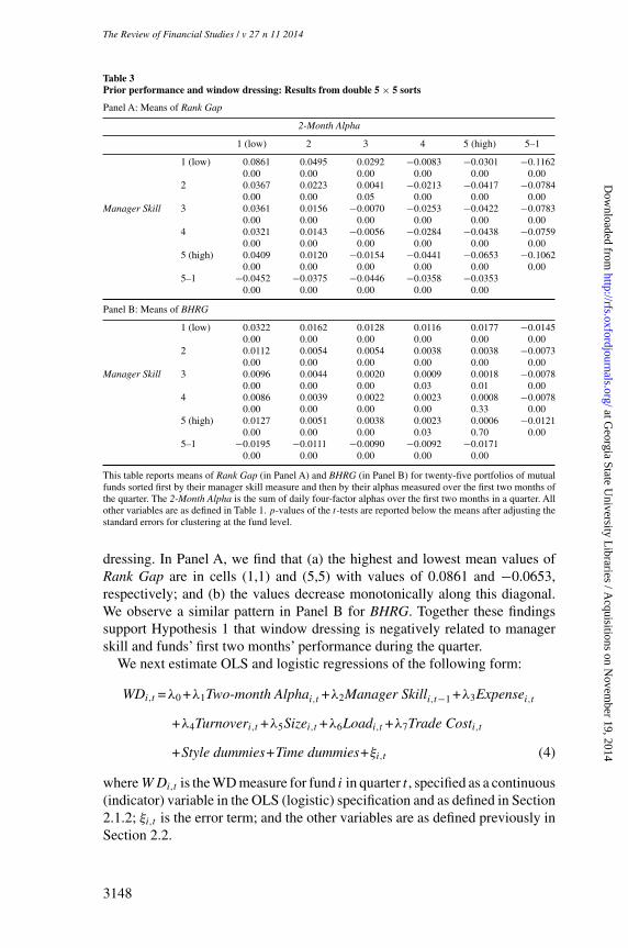
In Table 3, we present the results of our sorting analysis, where we firstsort funds into manager skill quintiles and then, within each skill quintile, sortfunds into performance (2-Month Alpha) quintiles. Panels A and B report theaverages of Rank Gap and BHRG for the twenty-five double-sorted portfolios.In both panels, controlling for managerial skill, as we move by rows from thelowest to highest performance quintile, the average WD measure is generallymonotonically decreasing. Similarly, controlling for performance, as we moveby columns from the lowest to highest skill quintile, the average WD measureagain is generally monotonically decreasing.Also, the (5–1) differences for boththe extreme performance and skill quintiles are all highly significant. Further,we can observe the interaction effects of skill and performance on window

3147

at Georgia State U




Dow

nloaded from


[18:05 9/10/2014 RFS-hhu045.tex] Page: 3148 3133–3170


Table 3Prior performance and window dressing: Results from double 5 × 5 sorts

Panel A: Means of Rank Gap

2-Month Alpha

1 (low) 2 3 4 5 (high) 5–1

1 (low) 0.0861 0.0495 0.0292 −0.0083 −0.0301 −0.11620.00 0.00 0.00 0.00 0.00 0.00

2 0.0367 0.0223 0.0041 −0.0213 −0.0417 −0.07840.00 0.00 0.05 0.00 0.00 0.00

Manager Skill 3 0.0361 0.0156 −0.0070 −0.0253 −0.0422 −0.07830.00 0.00 0.00 0.00 0.00 0.00

4 0.0321 0.0143 −0.0056 −0.0284 −0.0438 −0.07590.00 0.00 0.00 0.00 0.00 0.00

5 (high) 0.0409 0.0120 −0.0154 −0.0441 −0.0653 −0.10620.00 0.00 0.00 0.00 0.00 0.00

5–1 −0.0452 −0.0375 −0.0446 −0.0358 −0.03530.00 0.00 0.00 0.00 0.00

Panel B: Means of BHRG

1 (low) 0.0322 0.0162 0.0128 0.0116 0.0177 −0.01450.00 0.00 0.00 0.00 0.00 0.00

2 0.0112 0.0054 0.0054 0.0038 0.0038 −0.00730.00 0.00 0.00 0.00 0.00 0.00

Manager Skill 3 0.0096 0.0044 0.0020 0.0009 0.0018 −0.00780.00 0.00 0.00 0.03 0.01 0.00

4 0.0086 0.0039 0.0022 0.0023 0.0008 −0.00780.00 0.00 0.00 0.00 0.33 0.00

5 (high) 0.0127 0.0051 0.0038 0.0023 0.0006 −0.01210.00 0.00 0.00 0.03 0.70 0.00

5–1 −0.0195 −0.0111 −0.0090 −0.0092 −0.01710.00 0.00 0.00 0.00 0.00

This table reports means of Rank Gap (in Panel A) and BHRG (in Panel B) for twenty-five portfolios of mutualfunds sorted first by their manager skill measure and then by their alphas measured over the first two months ofthe quarter. The 2-Month Alpha is the sum of daily four-factor alphas over the first two months in a quarter. Allother variables are as defined in Table 1. p-values of the t-tests are reported below the means after adjusting thestandard errors for clustering at the fund level.

dressing. In Panel A, we find that (a) the highest and lowest mean values ofRank Gap are in cells (1,1) and (5,5) with values of 0.0861 and −0.0653,respectively; and (b) the values decrease monotonically along this diagonal.We observe a similar pattern in Panel B for BHRG. Together these findingssupport Hypothesis 1 that window dressing is negatively related to managerskill and funds’ first two months’ performance during the quarter.

We next estimate OLS and logistic regressions of the following form:

WDi,t =λ0 +λ1Two-month Alphai,t +λ2Manager Skilli,t−1 +λ3Expensei,t

+λ4Turnoveri,t +λ5Sizei,t +λ6Loadi,t +λ7Trade Costi,t

+Style dummies+Time dummies+ξi,t (4)

whereWDi,t is the WD measure for fund i in quarter t , specified as a continuous(indicator) variable in the OLS (logistic) specification and as defined in Section2.1.2; ξi,t is the error term; and the other variables are as defined previously inSection 2.2.

3148

at Georgia State U




Dow

nloaded from


[18:05 9/10/2014 RFS-hhu045.tex] Page: 3149 3133–3170


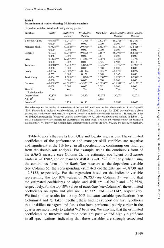
Table 4Determinants of window dressing: Multivariate analysis

Dependent variable: Window dressing during quarter t

Variables BHRG BHRG10% BHRG20% Rank Gap Rank Gap10% Rank Gap20%Dummy Dummy Dummy Dummy

2-Month Alphat −0.0902∗∗∗ −6.2419∗∗∗ −4.3338∗∗∗ −0.8738∗∗∗ −16.3321∗∗∗ −15.3831∗∗∗0.000 0.000 0.000 0.000 0.000 0.000

Manager Skillt-1 −0.7528∗∗∗ −39.3524∗∗∗ −29.6760∗∗∗ −2.3133∗∗∗ −39.1142∗∗∗ −33.5428∗∗∗0.000 0.000 0.000 0.000 0.000 0.000

Expenset 0.1033 76.2404∗∗∗ 49.8678∗∗∗ 0.4577 45.3936∗∗∗ 36.5311∗∗∗0.488 0.000 0.000 0.131 0.000 0.000

Sizet 0.1424∗∗∗ 12.2076∗∗∗ 11.3944∗∗∗ −0.0170 1.7436 1.47330.000 0.002 0.000 0.825 0.505 0.415

Turnovert 0.0688∗∗∗ 6.2330∗∗∗ 5.8776∗∗∗ 0.0735∗∗∗ 3.1782∗∗∗ 2.1908∗∗∗0.000 0.000 0.000 0.000 0.000 0.000

Loadt −0.0016 −0.3879∗∗∗ −0.1324 0.0051∗∗ −0.0709 0.02240.237 0.003 0.127 0.048 0.362 0.680

Trade Costt 0.0341∗∗∗ 1.6859∗∗∗ 1.8790∗∗∗ 0.0502∗∗∗ 1.0775∗∗∗ 0.9396∗∗∗0.000 0.000 0.000 0.000 0.000 0.000

Constant −0.0099∗∗∗ −4.5955∗∗∗ −3.3761∗∗∗ −0.0239∗∗∗ −3.6541∗∗∗ −2.5127∗∗∗0.008 0.000 0.000 0.002 0.000 0.000

Time & Yes Yes Yes Yes Yes YesStyle dummies

Observations 30,874 30,874 30,874 30,072 30,072 30,072Adj. R2 0.172 0.103Pseudo R2 0.178 0.136 0.0916 0.0677

This table reports the results of regressions of the two WD measures on fund characteristics. Rank Gap10%(20%) Dummy is an indicator variable defined as 1 if Rank Gap is in the top 10th (20th) percentile for a givenquarter, and 0 otherwise; and BHRG10% (20%) Dummy is an indicator variable defined as 1 if BHRG is in thetop 10th (20th) percentile for a given quarter, and 0 otherwise. All other variables are as defined in Tables 1, 2,and 3. Standard errors are adjusted for clustering at the fund level. p-values are reported below the estimatedcoefficients. *, **, and *** denote significant differences from zero at the 10%, 5%, and 1% levels, respectively.

Table 4 reports the results from OLS and logistic regressions. The estimatedcoefficients of the performance and manager skill variables are negativeand significant at the 1% level in all specifications, confirming our findingsfrom the double-sort analysis. For example, using the continuous form ofthe BHRG measure (see Column 2), the estimated coefficient on 2-monthAlpha is −0.0902, and on manager skill it is −0.7528. Similarly, when usingthe continuous form of the Rank Gap measure as the dependent variable(see Column 5), the corresponding estimated coefficients are −0.8738 and−2.3133, respectively. For the regression based on the indicator variablerepresenting the top 10% values of BHRG (see Column 3), we find thatthe estimated coefficients on alpha and skill are −6.2419 and −39.3524,respectively. For the top 10% values of Rank Gap (see Column 6), the estimatedcoefficients on alpha and skill are −16.3321 and −39.1142, respectively.We find similar results for the top 20% indicator variable specifications (seeColumns 4 and 7). Taken together, these findings support our first hypothesisthat unskilled managers and funds that have performed poorly earlier in thequarter are more likely to exhibit WD behavior. We also find that the estimatedcoefficients on turnover and trade costs are positive and highly significantin all specifications, indicating that these variables are strongly associated

3149

at Georgia State U




Dow

nloaded from


[18:05 9/10/2014 RFS-hhu045.tex] Page: 3150 3133–3170


with WD behavior. We further investigate these associations in the followingsections.

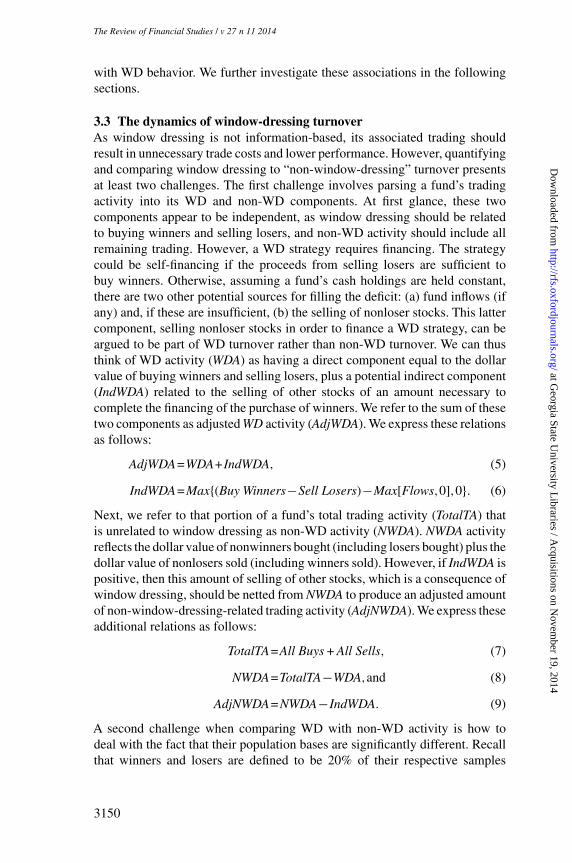
3.3 The dynamics of window-dressing turnoverAs window dressing is not information-based, its associated trading shouldresult in unnecessary trade costs and lower performance. However, quantifyingand comparing window dressing to “non-window-dressing” turnover presentsat least two challenges. The first challenge involves parsing a fund’s tradingactivity into its WD and non-WD components. At first glance, these twocomponents appear to be independent, as window dressing should be relatedto buying winners and selling losers, and non-WD activity should include allremaining trading. However, a WD strategy requires financing. The strategycould be self-financing if the proceeds from selling losers are sufficient tobuy winners. Otherwise, assuming a fund’s cash holdings are held constant,there are two other potential sources for filling the deficit: (a) fund inflows (ifany) and, if these are insufficient, (b) the selling of nonloser stocks. This lattercomponent, selling nonloser stocks in order to finance a WD strategy, can beargued to be part of WD turnover rather than non-WD turnover. We can thusthink of WD activity (WDA) as having a direct component equal to the dollarvalue of buying winners and selling losers, plus a potential indirect component(IndWDA) related to the selling of other stocks of an amount necessary tocomplete the financing of the purchase of winners. We refer to the sum of thesetwo components as adjusted WD activity (AdjWDA). We express these relationsas follows:

AdjWDA=WDA+IndWDA, (5)

IndWDA=Max(Buy Winners−Sell Losers)−Max[Flows,0],0. (6)

Next, we refer to that portion of a fund’s total trading activity (TotalTA) thatis unrelated to window dressing as non-WD activity (NWDA). NWDA activityreflects the dollar value of nonwinners bought (including losers bought) plus thedollar value of nonlosers sold (including winners sold). However, if IndWDA ispositive, then this amount of selling of other stocks, which is a consequence ofwindow dressing, should be netted from NWDA to produce an adjusted amountof non-window-dressing-related trading activity (AdjNWDA). We express theseadditional relations as follows:

TotalTA=All Buys + All Sells, (7)

NWDA=TotalTA−WDA,and (8)

AdjNWDA=NWDA−IndWDA. (9)

A second challenge when comparing WD with non-WD activity is how todeal with the fact that their population bases are significantly different. Recallthat winners and losers are defined to be 20% of their respective samples

3150

at Georgia State U




Dow

nloaded from


[18:05 9/10/2014 RFS-hhu045.tex] Page: 3151 3133–3170


while nonwinners and nonlosers constitute the other 80%. Thus, a fund isexpected to have, on average, activity in nonwinner and nonloser stocks thatis approximately four times as large as its activity in winner and loser stocks.To address this issue, for each fund quarter we compute the following fourturnover ratios, wherein the various trading activity measures are scaled by thefund’s TNA: WDA/TNA and NWDA/TNA, and AdjWDA/TNA and AdjNWDA/TNA. The first pair of ratios ignores the indirect WD effect, while the latter pairof ratios accounts for this effect. We posit that the portion of overall turnoverattributable to buying winners and selling losers should be relatively higherfor window dressers than for non–window dressers. To test this conjecture, wedivide the respective pairs of ratios to get WDA/NWDA and AdjWDA/AdjNWDAand argue that these ratios should be the highest for window dressers.

We report the findings in Table 5. In Panel A, we sort funds on BHRG andreport the averages of the turnover measures for each decile. We observe thatthe direct measure of WD activity (WDA) is the highest for funds in decile 10(19.1%). Moreover, we observe that the indirect WD activity turnover (IWDA)is also the highest in decile 10 (8.1%). This indirect activity is an economicallylarge component of turnover, and suggests that window dressers do not solelyrely on selling losers to buy winners, but also on selling substantial amounts ofother stocks. We also report averages for non-window-dressing-related turnover(see columns NWDA and AdjNWDA), which are significantly larger than thosefor WD-related turnover (by a factor of about four for the entire sample).We also observe that the non-WD-related turnover is the highest in decile 10,suggesting that window dressers also have a higher turnover in other stocks.Still, as indicated in the columnWDA/NWDA, where we take the ratio of windowdressing to non-window-dressing-related turnover, we observe that relative WDactivity remains the largest in decile 10. Thus, while window dressers appearto have higher rates of turnover reflecting their information-less trading, theyengage in even higher relative rates of turnover of winner and loser stocks.This effect is even more pronounced when we adjust for indirect WD activity,as shown in the last column. We find similar results in Panel B for sorts usingRank Gap.

3.4 Window dressing and trade costsThe above finding that window dressing is positively related to turnoversuggests that it should also be associated with higher trade costs. To investigatethe magnitude of these costs, we compute for each fund each quarter the tradecosts (explicit, implicit, and total) associated with the buying of winners, theselling of losers, and the sum of the two activities. We then sort funds into WDdeciles and compute averages of the various trade costs for each decile. Theseresults are presented in Panels A and B of Table 6 for BHRG and Rank Gap,respectively.

In each panel, the highest level of total trade costs is observed for funds inthe highest WD decile 10. Under column heading “Buy Winner + Sell Loser

3151

at Georgia State U




Dow

nloaded from


[18:05 9/10/2014 RFS-hhu045.tex] Page: 3152 3133–3170


Table 5Window-dressing trade activity

Panel A

BHRG decile WDA NWDA WDANWDA

IndWDA AdjWDA AdjNWDA AdjWDAAdjNWDA

1 (low) 0.074 0.380 0.198 0.010 0.086 0.368 0.2502 0.057 0.304 0.184 0.010 0.069 0.293 0.2423 0.047 0.256 0.185 0.008 0.056 0.247 0.2474 0.044 0.220 0.197 0.008 0.052 0.211 0.2665 0.045 0.217 0.208 0.010 0.055 0.207 0.2976 0.050 0.228 0.232 0.011 0.061 0.217 0.3377 0.065 0.259 0.267 0.015 0.080 0.243 0.3958 0.083 0.300 0.308 0.021 0.105 0.278 0.4769 0.112 0.347 0.356 0.031 0.144 0.315 0.56310 (high) 0.191 0.452 0.460 0.081 0.275 0.367 0.935

10–1 0.117 0.073 0.262 0.071 0.188 0.000 0.685

p-value 0.00 0.00 0.00 0.00 0.00 0.98 0.00

Panel B

Rank Gap decile WDA NWDA WDANWDA

IndWDA AdjWDA AdjNWDA AdjWDAAdjNWDA

1 (low) 0.079 0.343 0.231 0.016 0.097 0.326 0.3382 0.072 0.290 0.247 0.018 0.091 0.271 0.3783 0.070 0.278 0.248 0.017 0.088 0.260 0.3824 0.067 0.267 0.252 0.018 0.086 0.248 0.3905 0.066 0.262 0.249 0.018 0.085 0.244 0.3926 0.067 0.266 0.250 0.019 0.087 0.247 0.3877 0.066 0.276 0.240 0.016 0.083 0.259 0.3458 0.070 0.284 0.257 0.016 0.086 0.268 0.3639 0.082 0.313 0.275 0.020 0.104 0.291 0.40910 (high) 0.129 0.392 0.343 0.046 0.176 0.345 0.605

10–1 0.050 0.049 0.112 0.029 0.079 0.020 0.266

p-value 0.00 0.00 0.00 0.00 0.00 0.013 0.00

This table reports the means of components of WD trade activity for decile portfolios of mutual funds sorted bythe two WD measures (BHRG in Panel A and Rank Gap in Panel B) for each quarter. WDA is a direct componentof WD activity given by the dollar value of buying winners and selling losers. NWDA is non-WD activity givenby the dollar value of nonwinners bought (including losers bought) plus the dollar value of nonlosers sold(including winners sold). IndWDA refers to an indirect component of WD activity given by the sell value of otherstocks necessary to complete the financing of the purchase of winners. The sum of WDA and IndWDA is definedas adjusted WD activity (AdjWDA). AdjNWDA is defined as NWDA subtracted by IndWDA. All trade activityvariables are scaled by beginning-of-the-quarter assets. p-values of the t-tests of the differences for deciles 10and 1 are reported in the last row of the two panels after adjusting the standard errors for clustering at the fundlevel.

Cost,” the estimates are 14.4 and 10.3 basis points for BHRG and Rank Gap,respectively. We note that these are quarterly trade costs and relate only to thebuying of winners and selling of losers, and do not include the costs relatedto indirect WD activity. Also, when we examine the two components of tradecost, we find that higher implicit costs appear to drive these results more thanexplicit costs. Since the Abel Noser database does not provide the identitiesof the trading institutions, we cannot conclusively attribute the higher implicitcosts to the urgency of window dressers to trade (buy winners and sell losers)near quarter-ends. Nevertheless, if one assumes that there is a predominanceof window dressers in the aggregate trading of winners and losers, then thiscan be a possibility. Overall, this evidence suggests that window dressing isassociated with higher trade costs.

3152

at Georgia State U




Dow

nloaded from


[18:05 9/10/2014 RFS-hhu045.tex] Page: 3153 3133–3170


Table 6Window-dressing trade costs

Panel A

Buy winner cost Sell loser cost Buy winner + sell loser cost

BHRG decile Total Explicit Implicit Total Explicit Implicit Total Explicit Implicit

1 (low) 0.00035 0.00007 0.00027 0.00028 0.00006 0.00022 0.00063 0.00013 0.000492 0.00027 0.00005 0.00022 0.00020 0.00004 0.00016 0.00047 0.00009 0.000383 0.00021 0.00004 0.00017 0.00017 0.00003 0.00014 0.00038 0.00007 0.000314 0.00020 0.00003 0.00016 0.00015 0.00003 0.00012 0.00034 0.00006 0.000285 0.00021 0.00004 0.00018 0.00014 0.00003 0.00011 0.00035 0.00006 0.000296 0.00023 0.00004 0.00019 0.00014 0.00003 0.00012 0.00038 0.00007 0.000317 0.00030 0.00005 0.00025 0.00018 0.00003 0.00015 0.00048 0.00008 0.000408 0.00041 0.00007 0.00034 0.00023 0.00004 0.00019 0.00064 0.00010 0.000539 0.00058 0.00009 0.00049 0.00027 0.00004 0.00023 0.00085 0.00013 0.0007110 (high) 0.00113 0.00018 0.00095 0.00031 0.00005 0.00026 0.00144 0.00023 0.00120

10–1 0.00079 0.00011 0.00067 0.00003 −0.00001 0.00004 0.00081 0.00010 0.0007

p-value 0.00 0.00 0.00 0.04 0.00 0.00 0.00 0.00 0.00

Panel B

Rank Gapdecile

Buy winner cost Sell loser cost Buy winner + sell loser cost

Total Explicit Implicit Total Explicit Implicit Total Explicit Implicit

1 (low) 0.00040 0.00007 0.00032 0.00022 0.00004 0.00018 0.00062 0.00012 0.000502 0.00037 0.00007 0.00030 0.00017 0.00003 0.00014 0.00054 0.00010 0.000443 0.00037 0.00006 0.00030 0.00016 0.00003 0.00013 0.00052 0.00009 0.000434 0.00034 0.00006 0.00028 0.00016 0.00003 0.00013 0.00050 0.00009 0.000415 0.00033 0.00005 0.00027 0.00015 0.00003 0.00012 0.00048 0.00008 0.000406 0.00035 0.00006 0.00029 0.00019 0.00003 0.00015 0.00053 0.00009 0.000447 0.00030 0.00005 0.00025 0.00021 0.00004 0.00017 0.00051 0.00009 0.000428 0.00032 0.00005 0.00027 0.00023 0.00004 0.00019 0.00055 0.00009 0.000459 0.00039 0.00007 0.00032 0.00027 0.00005 0.00023 0.00066 0.00011 0.0005510 (high) 0.00071 0.00011 0.00059 0.00032 0.00005 0.00027 0.00103 0.00017 0.00086

10–1 0.00031 0.00004 0.00027 0.00010 0.00001 0.00009 0.00042 0.00005 0.00037

p-value 0.00 0.00 0.00 0.00 0.00 0.00 0.00 0.00 0.00

This table reports average trade costs associated with the buying of winners and selling of losers during a quarterfor decile portfolios of mutual funds sorted by the two WD measures (BHRG in Panel A and Rank Gap in PanelB) for each quarter. To compute funds’ trade costs in a given fund quarter, we first compute a fund’s buys andsells of each stock traded during the quarter by comparing the fund’s beginning- and end-of-quarter holdings. Wethen use the Abel Noser database to identify all institutions’ buys and sells of each stock in the same matchingquarter. For each trade (keeping buys and sells separate), we compute the explicit trade cost per share by dividingthe reported trade commission by the number of shares in the transaction. We also compute the implicit tradecost per share for buys (sells) as the difference between the reported transaction price (open price) and the stock’sopening price (transaction price) that day. The total trade cost per share is computed as the sum of the explicitand implicit trade costs. Then, for all trades of the stock during the quarter, we compute separately for buys andsells the volume-weighted explicit, implicit, and total trade costs per share. We repeat these calculations for eachstock traded by funds in the quarter. Following this, we then link these trade costs to a fund’s buys and sellsduring the quarter and compute for each trade the explicit, implicit, and total trade costs by multiplying the tradecosts per share by the trade size. We then sum the trade costs for all trades during quarter to obtain the total dollartrade costs, which we then scale by the funds’ beginning-of-quarter assets under management. p-values of thet-tests of the differences for deciles 10 and 1 are reported in the last row after adjusting the standard errors forclustering at the fund level.

4. Window Dressing versus Momentum Trading

While window dressing and momentum trading share similar traits in that bothinvolve buying winners and selling losers, our findings so far support that ourmeasures are capturing window dressing, as they are negatively correlated with

3153

at Georgia State U




Dow

nloaded from


[18:05 9/10/2014 RFS-hhu045.tex] Page: 3154 3133–3170


fund’s past performance and manager skill (Hypothesis 1). We conduct twotypes of seasonality tests, intraquarter and December, to distinguish betweenwindow dressing and information-motivated momentum trading.

4.1 Intraquarter testsWe examine the intraquarter exposure of a fund’s returns to its reported winnerstocks. For momentum traders, this exposure should be uniformly distributedacross months due to the monthly updating of winner stocks inherent in thestrategy. That is, a momentum trader should buy winners and sell losers on arolling basis. Consider, for example, a momentum trader who discloses holdingson the March quarterly cycle. Given the holding period of a typical momentumtrader, winners acquired in January, February, and March will have a stronglikelihood of still being held and thus reported at March end. For a windowdresser, winner stocks are only acquired periodically at fiscal quarter month-ends, for example, in March. Thus, window dressers’ exposure to winnersshould be systematically higher in the third month of a quarter.11

To test this conjecture, we estimate this exposure for each fund month bycomputing the correlation over the month between a fund’s daily returns and thedaily returns on the portfolio of recent winner stocks held by the fund. Recentwinners are determined over the three-month period ending each month andare updated on a monthly basis. To determine if winners are actually held by afund at month-end, we use the fund’s reported quarter-end holdings to proxyfor month-end holdings. We believe that any noise introduced by this proxyshould bias us against finding results consistent with our conjecture. We thenestimate the following regression:

Corri,t =α0 +α1WDi,t +α2WDi,t×I(FQEM)i,t +α3I(FQEM)i,t

+Style dummies+ηi,t (10)

where Corri,t is the correlation between daily fund returns and daily returnsof winner stocks held by the fund i in month t ; I (FQEM)i,t is an indicatorvariable that takes a value of 1 for fund i if month t is a fiscal quarter-endingmonth, and 0 otherwise; and ηi,t is the error term. For window dressers, unlikemomentum traders, the monthly correlation should increase systematicallyduring the month corresponding to the fiscal quarter-end, that is, α2 shouldbe greater than zero. From results in Table 7, we observe that the estimatedcoefficient α2 is positive and significant in all six specifications, except inmodel 1, where it is positive, but not significant.

4.2 December testsThe literature on tournaments and the flow-performance relation (e.g., seeBrown, Harlow, and Starks 1996; Chevalier and Ellison 1997; Sirri and Tufano

11 We thank Clemens Sialm for directing us to this conjecture.

3154

at Georgia State U




Dow

nloaded from


[18:05 9/10/2014 RFS-hhu045.tex] Page: 3155 3133–3170


Table 7Intraquarter variability in fund exposure to winner stocks

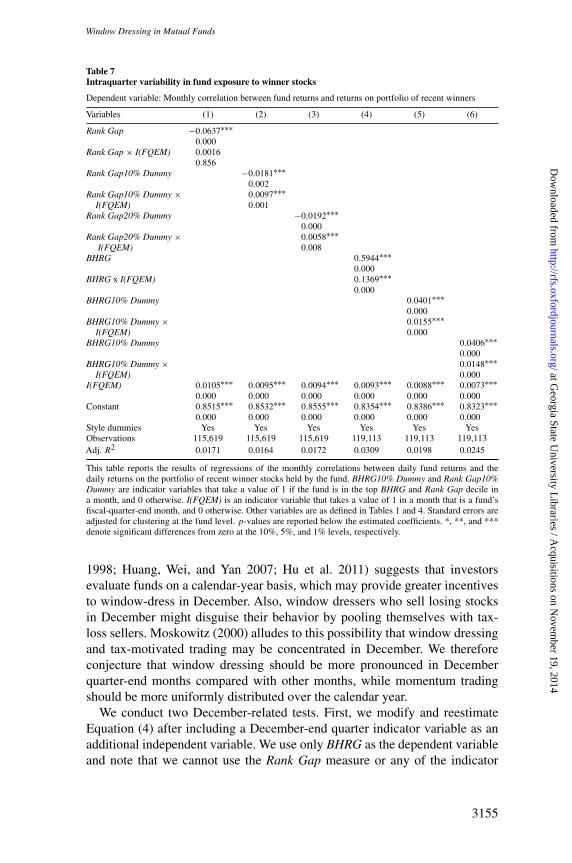
Dependent variable: Monthly correlation between fund returns and returns on portfolio of recent winners

Variables (1) (2) (3) (4) (5) (6)

Rank Gap −0.0637∗∗∗0.000

Rank Gap × I(FQEM) 0.00160.856

Rank Gap10% Dummy −0.0181∗∗∗0.002

Rank Gap10% Dummy × 0.0097∗∗∗I(FQEM) 0.001

Rank Gap20% Dummy −0.0192∗∗∗0.000

Rank Gap20% Dummy × 0.0058∗∗∗I(FQEM) 0.008

BHRG 0.5944∗∗∗0.000

BHRG x I(FQEM) 0.1369∗∗∗0.000

BHRG10% Dummy 0.0401∗∗∗0.000

BHRG10% Dummy × 0.0155∗∗∗I(FQEM) 0.000

BHRG10% Dummy 0.0406∗∗∗0.000

BHRG10% Dummy × 0.0148∗∗∗I(FQEM) 0.000

I(FQEM) 0.0105∗∗∗ 0.0095∗∗∗ 0.0094∗∗∗ 0.0093∗∗∗ 0.0088∗∗∗ 0.0073∗∗∗0.000 0.000 0.000 0.000 0.000 0.000

Constant 0.8515∗∗∗ 0.8532∗∗∗ 0.8555∗∗∗ 0.8354∗∗∗ 0.8386∗∗∗ 0.8323∗∗∗0.000 0.000 0.000 0.000 0.000 0.000

Style dummies Yes Yes Yes Yes Yes YesObservations 115,619 115,619 115,619 119,113 119,113 119,113Adj. R2 0.0171 0.0164 0.0172 0.0309 0.0198 0.0245

This table reports the results of regressions of the monthly correlations between daily fund returns and thedaily returns on the portfolio of recent winner stocks held by the fund. BHRG10% Dummy and Rank Gap10%Dummy are indicator variables that take a value of 1 if the fund is in the top BHRG and Rank Gap decile ina month, and 0 otherwise. I(FQEM) is an indicator variable that takes a value of 1 in a month that is a fund’sfiscal-quarter-end month, and 0 otherwise. Other variables are as defined in Tables 1 and 4. Standard errors areadjusted for clustering at the fund level. p-values are reported below the estimated coefficients. *, **, and ***denote significant differences from zero at the 10%, 5%, and 1% levels, respectively.

1998; Huang, Wei, and Yan 2007; Hu et al. 2011) suggests that investorsevaluate funds on a calendar-year basis, which may provide greater incentivesto window-dress in December. Also, window dressers who sell losing stocksin December might disguise their behavior by pooling themselves with tax-loss sellers. Moskowitz (2000) alludes to this possibility that window dressingand tax-motivated trading may be concentrated in December. We thereforeconjecture that window dressing should be more pronounced in Decemberquarter-end months compared with other months, while momentum tradingshould be more uniformly distributed over the calendar year.

We conduct two December-related tests. First, we modify and reestimateEquation (4) after including a December-end quarter indicator variable as anadditional independent variable. We use only BHRG as the dependent variableand note that we cannot use the Rank Gap measure or any of the indicator

3155

at Georgia State U




Dow

nloaded from


[18:05 9/10/2014 RFS-hhu045.tex] Page: 3156 3133–3170


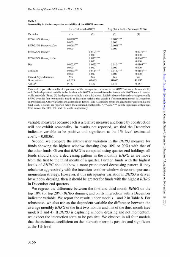
Table 8Seasonality in the intraquarter variability of the BHRG measure

1st – 3rd month BHRG Avg.(1st + 2nd) – 3rd month BHRG

Variables (1) (2) (3) (4)

BHRG10% Dummy 0.0128∗∗∗ 0.0095∗∗∗0.000 0.000

BHRG10% Dummy x Dec 0.0068∗∗∗ 0.0048∗∗∗0.000 0.000

BHRG20% Dummy 0.0104∗∗∗ 0.0076∗∗∗0.000 0.000

BHRG20% Dummy x Dec 0.0057∗∗∗ 0.0040∗∗∗0.000 0.000

Dec 0.0055∗∗∗ 0.0053∗∗∗ 0.0104∗∗∗ 0.0103∗∗∗0.000 0.000 0.000 0.000

Constant −0.0103∗∗∗ −0.0114∗∗∗ −0.0147∗∗∗ −0.0156∗∗∗0.000 0.000 0.000 0.000

Time & Style dummies Yes Yes Yes YesObservations 40,695 40,695 40,695 40,695Adj. R2 0.137 0.152 0.147 0.157

This table reports the results of regressions of the intraquarter variation in the BHRG measure. In models (1)and (2) the dependent variable is the third-month BHRG subtracted from the first-month BHRG in each quarter,while in models (3) and (4) the dependent variable is the third-month BHRG subtracted from the average monthlyBHRG over the first two months. Dec is an indicator variable that equals 1 if the reporting month is December,and 0 otherwise. Other variables are as defined in Tables 1 and 4. Standard errors are adjusted for clustering at thefund level. p-values are reported below the estimated coefficients. *, **, and *** denote significant differencesfrom zero at the 10%, 5%, and 1% levels, respectively.

variable measures because each is a relative measure and hence by constructionwill not exhibit seasonality. In results not reported, we find the Decemberindicator variable to be positive and significant at the 1% level (estimatedcoeff. = 0.0036).

Second, we compare the intraquarter variation in the BHRG measure forfunds showing the highest window dressing (top 10% or 20%) with that ofthe other funds. Given that BHRG is computed using quarter-end holdings, allfunds should show a decreasing pattern in the monthly BHRG as we movefrom the first to the third month of a quarter. Further, funds with the highestlevels of BHRG should show a more pronounced decreasing pattern if theyrebalance aggressively with the intention to either window-dress or to pursue amomentum strategy. However, if this intraquarter variation in BHRG is drivenby window dressing, then it should be greater for funds with the highest BHRGin December-end quarters.

We regress the difference between the first and third month BHRG on thetop 10% (or top 20%) BHRG dummy, and on its interaction with a Decemberindicator variable. We report the results under models 1 and 2 in Table 8. Forrobustness, we also use as the dependent variable the difference between theaverage monthly BHRG of the first two months and that of the third month (seemodels 3 and 4). If BHRG is capturing window dressing and not momentum,we expect the interaction term to be positive. We observe in all four modelsthat the estimated coefficient on the interaction term is positive and significantat the 1% level.

3156

at Georgia State U




Dow

nloaded from


[18:05 9/10/2014 RFS-hhu045.tex] Page: 3157 3133–3170


5. Investors’ Flow Response to Window Dressing

5.1 Discussion of rationale and empirical predictionsWe empirically examine how window dressing can exist in the presence ofrational investors. If investors can be misled by funds’ WD activity and resultin funds rewarded with higher flows, one should expect that all fund managerswill engage in such activity. In contrast, if investors are not deceived by windowdressing and punish such funds with lower flows, then one would expect thatno manager will engage in window dressing. This line of reasoning motivatesus to investigate how rational investors respond to window dressing.

As discussed earlier, fund managers may disclose portfolio holdings witha delay up to 60 days following the end of a quarter. At the end of thisdelay period, investors can observe the reported quarter-end portfolio holdingsand attribute any discrepancy with the fund’s quarterly performance to eitherwindow dressing or to an improvement in their security selection strategy.If a fund manager window-dresses, but then performs well during the delayperiod, the manager may receive the benefit of doubt from investors who mayattribute the good performance to security selection. As a result, this managerwill receive higher investor flows between the filing date and the subsequentfiling date compared with the managers who do not window-dress. However, ifthe WD manager fails to achieve good performance during the delay period, themanager is penalized with lower flows compared with non–window dressers.Figure 1 depicts the timeline showing the above sequence of events related toinvestor flows and performance.12

We test this conjecture by collecting data on funds’filing dates from N-Q andN-CSR filings that are electronically available in the SEC’s EDGAR databasegoing back to 1994. We compute investor flows between the filing date and thesubsequent filing date using a fund’s TNA on the two dates and return over theperiod, and scale by TNA as of the filing date.13 We divide these flows by thenumber of days between the two filing dates to compute average daily flow,which we then multiply by 90 to express on a quarterly basis. We estimate thefollowing regression:

QtrFlowi,t+1 =γ0 +γ1WD dummyi,t +γ2WD dummyi,t×GoodPerfi,t

+γ3GoodPerfi,t +γ4QtrAlphaTopi,t +γ5QtrAlphaMidi,t +γ6QtrAlphaBoti,t

+γ7Manager Skilli,t−1 +γ8Expensei,t +γ9Turnoveri,t +γ10Sizei,t +γ11Loadi,t

+γ12Trade Costi,t +Style dummies+Time dummies+ωi,t (11)

12 Some funds may decide to voluntarily disclose their portfolio holdings sooner than 60 days. Such a decision islikely to be strategic, as shown by Ge and Zheng (2006). Therefore, to the extent that early voluntary disclosurehas information, it should bias us against finding results using the performance during the entire 60-day delayperiod.

13 When TNA is not available for a particular date, we use the closest month-end figure adjusted for the returnsbetween that month end and the filing date.

3157

at Georgia State U




Dow

nloaded from


[18:05 9/10/2014 RFS-hhu045.tex] Page: 3158 3133–3170


whereQtrF lowi,t+1 represents the investor flows for fund i between the fund’sfiling date in quarter t+1 and its next quarter filing date, WDdummyi,t is anindicator variable that takes a value of 1 when the Rank Gap or BHRG measurefor fund i is either in the top 10% or in the top 20% of all funds in quarter t ,GoodPerfi,t is an indicator variable that equals 1 if the average daily return offund i over the delay period is positive and 0 otherwise, andQtrAlphaT opi,t ,QtrAlphaMidi,t , and QtrAlphaBoti,t are the top 20%, middle 60%, andbottom 20% performance quintiles for fund i in quarter t as defined in Sirri andTufano (1998). Note that in Equation (11) we use the indicator (rather than thecontinuous) forms of window dressing and performance so that we can comparethe levels of flows between window dressers and non–window dressers.

Our second hypothesis predicts that a manager benefits from windowdressing through higher incremental flows between the filing date and thenext quarter’s filing date if the manager performs well over the delay period.However, the manager incurs a cost in terms of lower incremental flows ifperformance is poor. Using the coefficient estimates from Equation (11), weillustrate in the following matrix the incremental flows for window dressersand non–window dressers corresponding to good and bad performance duringthe delay period.

Window dressers Non–window dressers Column diff.good performance γ1 +γ2 +γ3 γ3 γ1 +γ2bad performance γ1 0 γ1Row diff. γ2 +γ3 γ3

For good performance, the column difference in flows for window dressersand non–window dressers is (γ1 +γ2). The first prediction of our secondhypothesis is that this difference should be positive. In contrast, if performanceis bad, the column difference is simply γ1. The second prediction is that windowdressers will receive lower flows if they perform poorly, thus implying that γ1

should be negative. Together, these two predictions imply that window dressersare making a risky bet that performance during the delay period will be good.We test this by inspecting the row differences, which provide information onthe dispersion in payoffs between the two performance states (good and bad).If window dressers are indeed making a more risky bet, we expect γ2 +γ3>γ3,or γ2 to be positive.

5.2 Empirical resultsThe results from estimating Equation (11), reported in Table 9, are generallyconsistent with our arguments above. First, the estimated coefficient γ1 onthe WD Dummy is negative in the first four specifications, and significantat conventional levels in models 1, 3, and 4 (p-values of 0.001, 0.000, and0.002, respectively) and close to significant in model 2 (p-value of 0.109).This finding regarding the coefficient γ1 is consistent with the prediction thatwindow dressers attain lower flows when the delay period performance is poor.Second, the sum of the estimated coefficients on (a) the WD Dummy and (b) its

3158

at Georgia State U




Dow

nloaded from


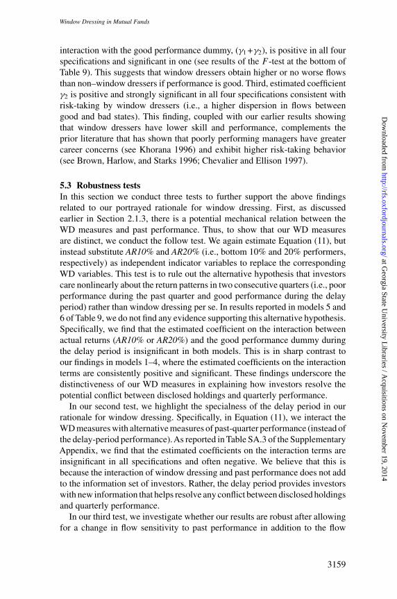
[18:05 9/10/2014 RFS-hhu045.tex] Page: 3159 3133–3170


interaction with the good performance dummy, (γ1 +γ2), is positive in all fourspecifications and significant in one (see results of the F -test at the bottom ofTable 9). This suggests that window dressers obtain higher or no worse flowsthan non–window dressers if performance is good. Third, estimated coefficientγ2 is positive and strongly significant in all four specifications consistent withrisk-taking by window dressers (i.e., a higher dispersion in flows betweengood and bad states). This finding, coupled with our earlier results showingthat window dressers have lower skill and performance, complements theprior literature that has shown that poorly performing managers have greatercareer concerns (see Khorana 1996) and exhibit higher risk-taking behavior(see Brown, Harlow, and Starks 1996; Chevalier and Ellison 1997).

5.3 Robustness testsIn this section we conduct three tests to further support the above findingsrelated to our portrayed rationale for window dressing. First, as discussedearlier in Section 2.1.3, there is a potential mechanical relation between theWD measures and past performance. Thus, to show that our WD measuresare distinct, we conduct the follow test. We again estimate Equation (11), butinstead substitute AR10% and AR20% (i.e., bottom 10% and 20% performers,respectively) as independent indicator variables to replace the correspondingWD variables. This test is to rule out the alternative hypothesis that investorscare nonlinearly about the return patterns in two consecutive quarters (i.e., poorperformance during the past quarter and good performance during the delayperiod) rather than window dressing per se. In results reported in models 5 and6 of Table 9, we do not find any evidence supporting this alternative hypothesis.Specifically, we find that the estimated coefficient on the interaction betweenactual returns (AR10% or AR20%) and the good performance dummy duringthe delay period is insignificant in both models. This is in sharp contrast toour findings in models 1–4, where the estimated coefficients on the interactionterms are consistently positive and significant. These findings underscore thedistinctiveness of our WD measures in explaining how investors resolve thepotential conflict between disclosed holdings and quarterly performance.

In our second test, we highlight the specialness of the delay period in ourrationale for window dressing. Specifically, in Equation (11), we interact theWD measures with alternative measures of past-quarter performance (instead ofthe delay-period performance).As reported in Table SA.3 of the SupplementaryAppendix, we find that the estimated coefficients on the interaction terms areinsignificant in all specifications and often negative. We believe that this isbecause the interaction of window dressing and past performance does not addto the information set of investors. Rather, the delay period provides investorswith new information that helps resolve any conflict between disclosed holdingsand quarterly performance.

In our third test, we investigate whether our results are robust after allowingfor a change in flow sensitivity to past performance in addition to the flow

3159

at Georgia State U




Dow

nloaded from




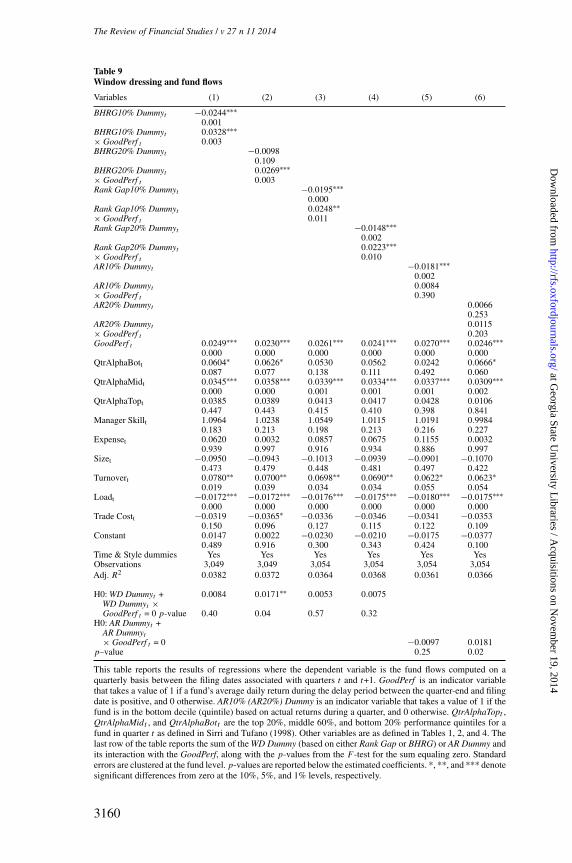
[18:05 9/10/2014 RFS-hhu045.tex] Page: 3160 3133–3170


Table 9Window dressing and fund flows

Variables (1) (2) (3) (4) (5) (6)

BHRG10% Dummyt −0.0244∗∗∗0.001

BHRG10% Dummyt 0.0328∗∗∗× GoodPerf t 0.003BHRG20% Dummyt −0.0098

0.109BHRG20% Dummyt 0.0269∗∗∗× GoodPerf t 0.003Rank Gap10% Dummyt −0.0195∗∗∗

0.000Rank Gap10% Dummyt 0.0248∗∗× GoodPerf t 0.011Rank Gap20% Dummyt −0.0148∗∗∗

0.002Rank Gap20% Dummyt 0.0223∗∗∗× GoodPerf t 0.010AR10% Dummyt −0.0181∗∗∗

0.002AR10% Dummyt 0.0084× GoodPerf t 0.390AR20% Dummyt 0.0066

0.253AR20% Dummyt 0.0115× GoodPerf t 0.203GoodPerf t 0.0249∗∗∗ 0.0230∗∗∗ 0.0261∗∗∗ 0.0241∗∗∗ 0.0270∗∗∗ 0.0246∗∗∗

0.000 0.000 0.000 0.000 0.000 0.000QtrAlphaBott 0.0604∗ 0.0626∗ 0.0530 0.0562 0.0242 0.0666∗

0.087 0.077 0.138 0.111 0.492 0.060QtrAlphaMidt 0.0345∗∗∗ 0.0358∗∗∗ 0.0339∗∗∗ 0.0334∗∗∗ 0.0337∗∗∗ 0.0309∗∗∗

0.000 0.000 0.001 0.001 0.001 0.002QtrAlphaTopt 0.0385 0.0389 0.0413 0.0417 0.0428 0.0106

0.447 0.443 0.415 0.410 0.398 0.841Manager Skillt 1.0964 1.0238 1.0549 1.0115 1.0191 0.9984

0.183 0.213 0.198 0.213 0.216 0.227Expenset 0.0620 0.0032 0.0857 0.0675 0.1155 0.0032

0.939 0.997 0.916 0.934 0.886 0.997Sizet −0.0950 −0.0943 −0.1013 −0.0939 −0.0901 −0.1070

0.473 0.479 0.448 0.481 0.497 0.422Turnovert 0.0780∗∗ 0.0700∗∗ 0.0698∗∗ 0.0690∗∗ 0.0622∗ 0.0623∗

0.019 0.039 0.034 0.034 0.055 0.054Loadt −0.0172∗∗∗ −0.0172∗∗∗ −0.0176∗∗∗ −0.0175∗∗∗ −0.0180∗∗∗ −0.0175∗∗∗

0.000 0.000 0.000 0.000 0.000 0.000Trade Costt −0.0319 −0.0365∗ −0.0336 −0.0346 −0.0341 −0.0353

0.150 0.096 0.127 0.115 0.122 0.109Constant 0.0147 0.0022 −0.0230 −0.0210 −0.0175 −0.0377

0.489 0.916 0.300 0.343 0.424 0.100Time & Style dummies Yes Yes Yes Yes Yes YesObservations 3,049 3,049 3,054 3,054 3,054 3,054Adj. R2 0.0382 0.0372 0.0364 0.0368 0.0361 0.0366

H0: WD Dummyt + 0.0084 0.0171∗∗ 0.0053 0.0075WD Dummyt ×GoodPerf t = 0 p-value 0.40 0.04 0.57 0.32

H0: AR Dummyt +AR Dummyt× GoodPerf t = 0 −0.0097 0.0181

p–value 0.25 0.02

This table reports the results of regressions where the dependent variable is the fund flows computed on aquarterly basis between the filing dates associated with quarters t and t+1. GoodPerf is an indicator variablethat takes a value of 1 if a fund’s average daily return during the delay period between the quarter-end and filingdate is positive, and 0 otherwise. AR10% (AR20%) Dummy is an indicator variable that takes a value of 1 if thefund is in the bottom decile (quintile) based on actual returns during a quarter, and 0 otherwise. QtrAlphaTopt ,QtrAlphaMidt , and QtrAlphaBott are the top 20%, middle 60%, and bottom 20% performance quintiles for afund in quarter t as defined in Sirri and Tufano (1998). Other variables are as defined in Tables 1, 2, and 4. Thelast row of the table reports the sum of the WD Dummy (based on either Rank Gap or BHRG) or AR Dummy andits interaction with the GoodPerf, along with the p-values from the F -test for the sum equaling zero. Standarderrors are clustered at the fund level. p-values are reported below the estimated coefficients. *, **, and *** denotesignificant differences from zero at the 10%, 5%, and 1% levels, respectively.

3160

at Georgia State U




Dow

nloaded from


[18:05 9/10/2014 RFS-hhu045.tex] Page: 3161 3133–3170


sensitivity to the delay-period performance. For this purpose, we modifyEquation (11) and include a three-way interaction term of WD Dummy, delayperiod performance, and past performance. In results reported in Table SA.4 ofthe SupplementaryAppendix, the estimated coefficient on the interaction term ispositive but insignificant in three of the four specifications, while insignificantlynegative in the other. This finding suggests that there is little evidence of anincrease in flow sensitivity to past performance due to window dressing. Moreimportantly, the estimated coefficient on the two-way interaction between WDDummy and delay-period performance continues to be positive and stronglysignificant in all four specifications. This shows that our main finding ofinvestors’ incremental flow response to window dressing and delay-periodperformance continues to hold.

Taken together, the results are consistent with our rationale for windowdressing. If fund performance during the delay period is good, investorsattribute the incongruence between holdings-based returns and actual returns toimproved security selection and reward the fund with higher flows. In contrast,if fund performance is bad, then investors attribute the incongruence to windowdressing and punish the fund with lower flows.

6. Window Dressing and Future Performance

Our above findings indicate that WD managers are generally value-destroyersdue to their excessive portfolio turnover and trade cost generation. Further,such managers appear to be unskilled and trade for noninformational reasons.As such we hypothesize that WD managers should exhibit, on average, poorfuture performance. To test this hypothesis, we analyze the future performanceof window dressers over the short term (i.e., the subsequent quarter) as wellas over the long term (i.e., one, two, and three years) after controlling for pastperformance (including poor past performance).

6.1 Future short-term performance6.1.1 Sorts analyses. We begin with a univariate analysis where funds aresorted each quarter into WD deciles. Using daily returns and trade information(as imputed from changes in holdings), we estimate funds’ quarterly alphasand total trade costs over the next quarter. For each decile, we compute andreport means of these variables in Table 10 (see Panel A for BHRG and PanelB for Rank Gap). For each WD measure, we observe that the alphas exhibit agenerally monotonically decreasing pattern as we move from the lowest to thehighest decile. This pattern suggests that greater window dressing is associatedwith lower subsequent performance. For the highest WD decile, next quarter’saverage alphas are −0.66% and −0.74% for BHRG and Rank Gap, respectively.Further, the differences in the mean alphas between the bottom and top deciles(10–1) are −0.63% and −0.57% for BHRG and Rank Gap, respectively, andboth are highly significant. We also observe that window dressers continue

3161

at Georgia State U




Dow

nloaded from




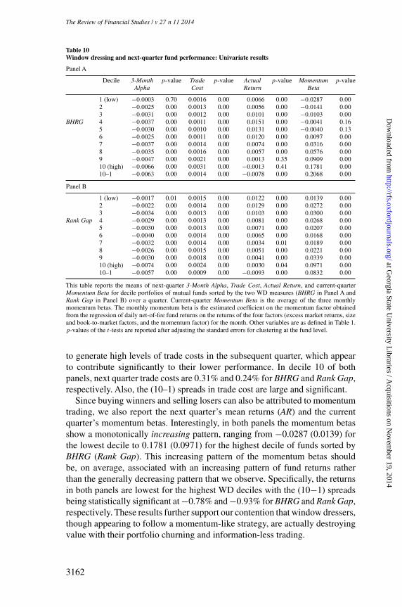
[18:05 9/10/2014 RFS-hhu045.tex] Page: 3162 3133–3170


Table 10Window dressing and next-quarter fund performance: Univariate results

Panel A

Decile 3-Month p-value Trade p-value Actual p-value Momentum p-valueAlpha Cost Return Beta

1 (low) −0.0003 0.70 0.0016 0.00 0.0066 0.00 −0.0287 0.002 −0.0025 0.00 0.0013 0.00 0.0056 0.00 −0.0141 0.003 −0.0031 0.00 0.0012 0.00 0.0101 0.00 −0.0103 0.00

BHRG 4 −0.0037 0.00 0.0011 0.00 0.0151 0.00 −0.0041 0.165 −0.0030 0.00 0.0010 0.00 0.0131 0.00 −0.0040 0.136 −0.0025 0.00 0.0011 0.00 0.0120 0.00 0.0097 0.007 −0.0037 0.00 0.0014 0.00 0.0074 0.00 0.0316 0.008 −0.0035 0.00 0.0016 0.00 0.0057 0.00 0.0576 0.009 −0.0047 0.00 0.0021 0.00 0.0013 0.35 0.0909 0.0010 (high) −0.0066 0.00 0.0031 0.00 −0.0013 0.41 0.1781 0.0010–1 −0.0063 0.00 0.0014 0.00 −0.0078 0.00 0.2068 0.00

Panel B

1 (low) −0.0017 0.01 0.0015 0.00 0.0122 0.00 0.0139 0.002 −0.0022 0.00 0.0014 0.00 0.0129 0.00 0.0272 0.003 −0.0034 0.00 0.0013 0.00 0.0103 0.00 0.0300 0.00

Rank Gap 4 −0.0029 0.00 0.0013 0.00 0.0081 0.00 0.0268 0.005 −0.0030 0.00 0.0013 0.00 0.0071 0.00 0.0207 0.006 −0.0040 0.00 0.0014 0.00 0.0065 0.00 0.0168 0.007 −0.0032 0.00 0.0014 0.00 0.0034 0.01 0.0189 0.008 −0.0026 0.00 0.0015 0.00 0.0051 0.00 0.0221 0.009 −0.0030 0.00 0.0018 0.00 0.0041 0.00 0.0339 0.0010 (high) −0.0074 0.00 0.0024 0.00 0.0030 0.04 0.0971 0.0010–1 −0.0057 0.00 0.0009 0.00 −0.0093 0.00 0.0832 0.00

This table reports the means of next-quarter 3-Month Alpha, Trade Cost, Actual Return, and current-quarterMomentum Beta for decile portfolios of mutual funds sorted by the two WD measures (BHRG in Panel A andRank Gap in Panel B) over a quarter. Current-quarter Momentum Beta is the average of the three monthlymomentum betas. The monthly momentum beta is the estimated coefficient on the momentum factor obtainedfrom the regression of daily net-of-fee fund returns on the returns of the four factors (excess market returns, sizeand book-to-market factors, and the momentum factor) for the month. Other variables are as defined in Table 1.p-values of the t-tests are reported after adjusting the standard errors for clustering at the fund level.

to generate high levels of trade costs in the subsequent quarter, which appearto contribute significantly to their lower performance. In decile 10 of bothpanels, next quarter trade costs are 0.31% and 0.24% for BHRG and Rank Gap,respectively. Also, the (10–1) spreads in trade cost are large and significant.

Since buying winners and selling losers can also be attributed to momentumtrading, we also report the next quarter’s mean returns (AR) and the currentquarter’s momentum betas. Interestingly, in both panels the momentum betasshow a monotonically increasing pattern, ranging from −0.0287 (0.0139) forthe lowest decile to 0.1781 (0.0971) for the highest decile of funds sorted byBHRG (Rank Gap). This increasing pattern of the momentum betas shouldbe, on average, associated with an increasing pattern of fund returns ratherthan the generally decreasing pattern that we observe. Specifically, the returnsin both panels are lowest for the highest WD deciles with the (10−1) spreadsbeing statistically significant at −0.78% and −0.93% for BHRG and Rank Gap,respectively. These results further support our contention that window dressers,though appearing to follow a momentum-like strategy, are actually destroyingvalue with their portfolio churning and information-less trading.

3162

at Georgia State U




Dow

nloaded from


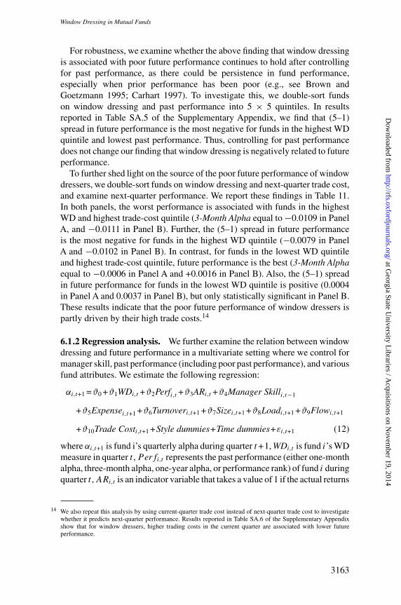
[18:05 9/10/2014 RFS-hhu045.tex] Page: 3163 3133–3170


For robustness, we examine whether the above finding that window dressingis associated with poor future performance continues to hold after controllingfor past performance, as there could be persistence in fund performance,especially when prior performance has been poor (e.g., see Brown andGoetzmann 1995; Carhart 1997). To investigate this, we double-sort fundson window dressing and past performance into 5 × 5 quintiles. In resultsreported in Table SA.5 of the Supplementary Appendix, we find that (5–1)spread in future performance is the most negative for funds in the highest WDquintile and lowest past performance. Thus, controlling for past performancedoes not change our finding that window dressing is negatively related to futureperformance.

To further shed light on the source of the poor future performance of windowdressers, we double-sort funds on window dressing and next-quarter trade cost,and examine next-quarter performance. We report these findings in Table 11.In both panels, the worst performance is associated with funds in the highestWD and highest trade-cost quintile (3-Month Alpha equal to −0.0109 in PanelA, and −0.0111 in Panel B). Further, the (5–1) spread in future performanceis the most negative for funds in the highest WD quintile (−0.0079 in PanelA and −0.0102 in Panel B). In contrast, for funds in the lowest WD quintileand highest trade-cost quintile, future performance is the best (3-Month Alphaequal to −0.0006 in Panel A and +0.0016 in Panel B). Also, the (5–1) spreadin future performance for funds in the lowest WD quintile is positive (0.0004in Panel A and 0.0037 in Panel B), but only statistically significant in Panel B.These results indicate that the poor future performance of window dressers ispartly driven by their high trade costs.14

6.1.2 Regression analysis. We further examine the relation between windowdressing and future performance in a multivariate setting where we control formanager skill, past performance (including poor past performance), and variousfund attributes. We estimate the following regression:

αi,t+1 =ϑ0 +ϑ1WDi,t +ϑ2Perfi,t +ϑ3ARi,t +ϑ4Manager Skilli,t−1

+ϑ5Expensei,t+1 +ϑ6Turnoveri,t+1 +ϑ7Sizei,t+1 +ϑ8Loadi,t+1 +ϑ9Flowi,t+1

+ϑ10Trade Costi,t+1 +Style dummies+Time dummies+εi,t+1 (12)

where αi,t+1 is fund i’s quarterly alpha during quarter t +1, WDi,t is fund i’s WDmeasure in quarter t ,Perfi,t represents the past performance (either one-monthalpha, three-month alpha, one-year alpha, or performance rank) of fund i duringquarter t ,ARi,t is an indicator variable that takes a value of 1 if the actual returns

14 We also repeat this analysis by using current-quarter trade cost instead of next-quarter trade cost to investigatewhether it predicts next-quarter performance. Results reported in Table SA.6 of the Supplementary Appendixshow that for window dressers, higher trading costs in the current quarter are associated with lower futureperformance.

3163

at Georgia State U




Dow

nloaded from





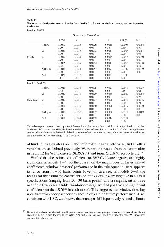
[18:05 9/10/2014 RFS-hhu045.tex] Page: 3164 3133–3170


Table 11Next-quarter fund performance: Results from double 5 × 5 sorts on window dressing and next-quartertrade costs

Panel A: BHRG

Next-quarter Trade Cost

1 (low) 2 3 4 5 (high) 5–1

1 (low) −0.0010 −0.0028 −0.0026 −0.0010 −0.0006 0.00040.29 0.00 0.00 0.28 0.60 0.79

2 −0.0029 −0.0036 −0.0033 −0.0041 −0.0028 0.00010.00 0.00 0.00 0.00 0.00 0.95

BHRG 3 −0.0007 −0.0022 −0.0025 −0.0029 −0.0048 −0.00400.20 0.00 0.00 0.00 0.00 0.00

4 −0.0015 −0.0029 −0.0042 −0.0047 −0.0033 −0.00180.03 0.00 0.00 0.00 0.00 0.12

5 (high) −0.0031 −0.0041 −0.0057 −0.0097 −0.0109 −0.00790.00 0.00 0.00 0.00 0.00 0.00

5–1 −0.0021 −0.0012 −0.0031 −0.0087 −0.01030.11 0.28 0.01 0.00 0.00

Panel B: Rank Gap

1 (low) −0.0021 −0.0038 −0.0035 −0.0021 0.0016 0.00370.32 0.00 0.00 0.02 0.15 0.01

2 −0.0023 −0.0040 −0.0029 −0.0039 −0.0027 −0.00040.00 0.00 0.00 0.00 0.01 0.78

Rank Gap 3 −0.0029 −0.0036 −0.0034 −0.0050 −0.0045 −0.00160.00 0.00 0.00 0.00 0.00 0.21

4 −0.0010 −0.0015 −0.0040 −0.0050 −0.0049 −0.00400.20 0.20 0.00 0.00 0.00 0.00

5 (high) −0.0009 −0.0028 −0.0047 −0.0066 −0.0111 −0.01020.23 0.00 0.00 0.00 0.00 0.00

5–1 0.0012 0.0009 −0.0012 −0.0044 −0.01270.31 0.38 0.26 0.00 0.00

This table reports means of next quarter 3-Month Alpha for twenty-five portfolios of mutual funds sorted firstby the two WD measures (BHRG in Panel A and Rank Gap in Panel B) and then by Trade Cost during the nextquarter. All variables are as defined in Table 1. p-values of the t-tests are reported below the means after adjustingthe standard errors for clustering at the fund level.

of fund i during quarter t are in the bottom decile and 0 otherwise, and all othervariables are as defined previously. We report the results from this estimationin Table 12 for WD measures BHRG10% and Rank Gap10%, respectively.15

We find that the estimated coefficients on BHRG10% are negative and highlysignificant in models 1−4. Further, based on the magnitudes of the estimatedcoefficients, window dressers’ performance in the subsequent quarter appearsto range from 40−60 basis points lower on average. In models 5−8, theresults for the estimated coefficients on Rank Gap10% are negative in all fourspecifications (ranging from 20−30 basis points) and are significant in threeout of the four cases. Unlike window dressing, we find positive and significantcoefficients on the AR10% in each model. This suggests that window dressingis distinct from poor past performance in explaining future performance. Also,consistent with KSZ, we observe that manager skill is positively related to future

15 Given that we have six alternative WD measures and four measures of past performance, for sake of brevity wepresent in Table 12 only the results for BHRG10% and Rank Gap10%. The findings for the other WD measuresare qualitatively similar.

3164

at Georgia State U




Dow

nloaded from


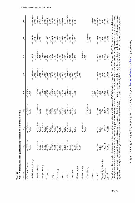
[18:05 9/10/2014 RFS-hhu045.tex] Page: 3165 3133–3170


Tabl

e12

Win

dow

dres

sing

and

next

-qua

rter

fund

perf

orm

ance

:M

ulti

vari

ate

resu

lts

Var

iabl

es(1

)(2

)(3

)(4

)(5

)(6

)(7

)(8

)

BH

RG

10%

Dum

my t

−0.0

052∗∗

∗−0.0

043∗∗

∗−0.0

058∗∗

∗−0.0

056∗∗

∗0.

000

0.00

00.

000

0.00

0R

ank

Gap

10%

Dum

my t

−0.0

028∗∗

∗−0.0

014

−0.0

018∗

−0.0

029∗∗

∗0.

002

0.11

50.

052

0.00

2A

R10

%D

umm

y t0.

0022

∗∗0.

0046

∗∗∗

0.00

31∗∗

∗0.

0027

∗∗0.

0029

∗∗∗

0.00

50∗∗

∗0.

0037

∗∗∗

0.00

25∗∗

0.02

70.

000

0.00

20.

011

0.00

40.

000

0.00

00.

018

Man

ager

Skill

t-1

0.27

43∗∗

0.23

43∗∗

0.27

92∗∗

0.28

85∗∗

∗0.

2440

∗∗0.

2916

∗∗∗

0.01

20.

027

0.01

20.

009

0.02

40.

008

Exp

ense

t+1

−0.0

031

−0.0

204

−0.0

726

−0.0

097

−0.0

340

−0.0

531

−0.1

066

−0.0

313

0.96

80.

778

0.30

90.

901

0.66

30.

476

0.14

70.

690

Size

t+1

0.03

17∗∗

0.03

11∗∗

0.00

590.

0246

∗0.

0202

0.02

09−0.0

024

0.02

040.

031

0.02

80.

673

0.09

70.

171

0.14

50.

862

0.17

0T

urno

ver t

+1

−0.0

022

−0.0

018

0.00

29−0.0

027

−0.0

038

−0.0

033

0.00

03−0.0

038

0.53

60.

610

0.39

90.

439

0.28

60.

344

0.93

30.

279

Loa

d t+

1−0.0

007

−0.0

006

−0.0

003

−0.0

007

−0.0

005

−0.0

004

−0.0

002

−0.0

006

0.18

50.

242

0.50

80.

201

0.33

00.

407

0.77

20.

311

Flow

t+1

0.04

60∗∗

∗0.

0435

∗∗∗

0.04

25∗∗

∗0.

0448

∗∗∗

0.04

49∗∗

∗0.

0425

∗∗∗

0.04

12∗∗

∗0.

0452

∗∗∗

0.00

00.

000

0.00

00.

000

0.00

00.

000

0.00

00.

000

Tra

deC

ost t+

1−0.0

023

−0.0

033

−0.0

059∗∗

−0.0

016

−0.0

033

−0.0

044∗

−0.0

066∗∗

∗−0.0

032

0.33

60.

167

0.01

50.

514

0.17

20.

073

0.00

70.

183

1-M

onth

Alp

hat

0.03

60∗∗

0.02

57∗

0.01

40.

093

3-M

onth

Alp

hat

0.08

11∗∗

∗0.

0766

∗∗∗

0.00

00.

000

1-Y

earA

lpha

t0.

0403

∗∗∗

0.03

92∗∗

∗0.

000

0.00

0Pe

rfR

ank t

−0.0

000

0.00

000.

437

0.88

0C

onst

ant

−0.0

024

−0.0

026

−0.0

011

−0.0

014

−0.0

014

−0.0

017

−0.0

004

−0.0

015

0.18

50.

130

0.53

20.

464

0.44

90.

344

0.81

30.

439

Tim

e&

Styl

edu

mm

ies

Yes

Yes

Yes

Yes

Yes

Yes

Yes

Yes

Obs

erva

tions

30,5

1229

,777

28,0

6929

,356

29,4

0828

,672

27,1

5529

,408

Adj

.R2

0.05

970.

0656

0.07

210.

0593

0.05

850.

0641

0.06

960.

0583

Thi

sta

ble

repo

rts

the

resu

ltsof

regr

essi

ons

ofth

e3-

Mon

thA

lpha

onth

etw

oW

Dm

easu

res

(BH

RG

10%

Dum

my

and

Ran

kG

ap10

%D

umm

y),A

R10

%D

umm

y,an

dva

riou

sfu

ndat

trib

utes

.T

hede

pend

ent

vari

able

is3-

Mon

thA

lpha

duri

ngth

ele

adin

gqu

arte

r.T

he1-

Mon

thA

lpha

and

1-Ye

arA

lpha

are

defin

edas

the

sum

offo

ur-f

acto

rda

ilyal

phas

over

the

quar

ter-

end

mon

th,

and

over

aye

arup

toth

equ

arte

r-en

d,re

spec

tivel

y.Pe

rfR

ank

isth

epe

rcen

tile

rank

ofa

fund

’squ

arte

rly

perf

orm

ance

.Oth

erva

riab

les

are

asde

fined

inTa

bles

1,4,

and

9.St

anda

rder

rors

are

adju

sted

forc

lust

erin

gat

the

fund

leve

l.p

-val

uesa

rere

port

edbe

low

the

estim

ated

coef

ficie

nts.

*,**

,and

***

deno

tesi

gnifi

cant

diff

eren

cesf

rom

zero

atth

e10

%,5

%,a

nd1%

leve

ls,r

espe

ctiv

ely.

3165

at Georgia State U




Dow

nloaded from


[18:05 9/10/2014 RFS-hhu045.tex] Page: 3166 3133–3170


performance. Together, the findings in this section support our third hypothesisthat window dressing is associated with lower future performance.

6.2 Long-term performanceWe sort funds each quarter into WD deciles, and compute the average one-,two-, and three-year alphas for each fund portfolio. The results, presented inTable 13, indicate a notable drop in fund performance in the highest WD deciles.To illustrate, for the BHRG-based results presented in Panel A, the one-, two-, and three-year alphas in decile 10 are −3.04%, −6.91%, and −11.36%,respectively. Further, the (10–1) decile differences are also all negative andhighly significant. Similar findings are observed in Panel B based on the RankGap measure.

To show that the above findings are distinct from poor past performance,we also sort funds on actual return (AR) and similarly compute the averagealphas over the next one, two, and three years. The results are reported in PanelC of Table 13.16 We find that the spreads in the future long-term alphas arealso negative and significant; however, the magnitude of the spreads is lessnegative than those reported in Panels A and B. We test this by conductinga difference-in-differences test based on (a) the spread between the extremedeciles of each WD measure, and (b) the spread between extreme AR deciles.As reported in Panel D, the difference-in-differences are significantly negative,indicating that the spreads between the extreme deciles of window dressingare more negative.17 We also analyze this issue in a multivariate setting byestimating the regression specification given in Equation (12) above, but usingas alternative dependent variables funds’ one-, two-, and three-year alphas. Inresults reported in Table SA.8 of the Supplementary Appendix, we continueto find that window dressing dominates poor past performance in explainingfuture long-term performance.

7. Concluding Remarks

We shed light on alleged window-dressing behavior of mutual fund managersusing a large sample of U.S. equity funds over the period September 1998to December 2008. We develop relative and absolute measures of windowdressing to capture the inconsistency between the information based onrealized fund returns and that based on disclosed portfolio holdings. Weconduct a battery of tests to show that these measures capture window-dressing behavior rather than momentum trading. Providing further support

16 Since window dressing is associated with poor past performance, we reverse the sorting order in Panel C suchthat the lowest (highest) AR decile in Panel C corresponds to the highest (lowest) WD decile in Panels A and B.

17 We also conduct a double-sort analysis where funds are sorted by window dressing and past performance (AR)into 5x5 quintiles. As reported in Table SA.7 of the Supplementary Appendix, we continue to find that windowdressing is negatively related to future long-term performance.

3166

at Georgia State U




Dow

nloaded from






[18:05 9/10/2014 RFS-hhu045.tex] Page: 3167 3133–3170


Table 13Window dressing and long-term fund performance: Univariate results

Panel A: BHRG

BHRG decile 1-Year Alpha 2-Year Alpha 3-Year Alpha

1 (low) −0.0094 −0.0189 −0.03252 −0.0116 −0.0221 −0.03533 −0.0103 −0.0207 −0.03264 −0.0121 −0.0233 −0.03585 −0.0115 −0.0231 −0.03416 −0.0115 −0.0254 −0.03727 −0.0131 −0.0258 −0.03778 −0.0162 −0.0327 −0.04929 −0.0194 −0.0401 −0.060710 (high) −0.0304 −0.0691 −0.113610–1 −0.0210 −0.0502 −0.0811p-value 0.00 0.00 0.00

Panel B: Rank Gap

Rank Gap decile 1-Year Alpha 2-Year Alpha 3-Year Alpha

1 (low) −0.0069 −0.0123 −0.02862 −0.0073 −0.0187 −0.03433 −0.0100 −0.0222 −0.03734 −0.0112 −0.0237 −0.03935 −0.0126 −0.0274 −0.04216 −0.0158 −0.0309 −0.04787 −0.0154 −0.0332 −0.05308 −0.0160 −0.0369 −0.05609 −0.0176 −0.0396 −0.061210 (high) −0.0332 −0.0601 −0.087310–1 −0.0263 −0.0477 −0.0587p-value 0.00 0.00 0.00

Panel C: AR

AR decile 1-Year Alpha 2-Year Alpha 3-Year Alpha

1 (high) −0.0076 −0.0143 −0.03232 −0.0089 −0.0221 −0.03923 −0.0089 −0.0234 −0.04124 −0.0125 −0.0264 −0.04405 −0.0121 −0.0280 −0.04736 −0.0141 −0.0287 −0.04737 −0.0149 −0.0311 −0.04878 −0.0183 −0.0358 −0.05419 −0.0221 −0.0442 −0.061210 (low) −0.0266 −0.0512 −0.067510–1 −0.0190 −0.0369 −0.0352p-value 0.00 0.00 0.00

Panel D: Difference-in-differences (10–1)

1-Year Alpha 2-Year Alpha 3-Year Alpha

BHRG – AR −0.0020 −0.0133 −0.0459p-value 0.59 0.03 0.00Rank Gap – AR −0.0073 −0.0108 −0.0235p-value 0.00 0.01 0.00

This table reports the means of long-term mutual fund performance subsequent to their WD activity for decileportfolios of mutual funds sorted by the two WD measures (BHRG in Panel A and Rank Gap in Panel B), andactual returns (AR in Panel C) for each quarter. The 1-Year Alpha is defined as the sum of four-factor daily alphasover the one year up to the quarter-end. The 2-Year Alpha is defined as the sum of four-factor daily alphas overthe two years up to the quarter-end. The 3-Year Alpha is defined as the sum of four-factor daily alphas over thethree years up to the quarter-end. p-values of the t-tests of the differences for deciles 10 and 1 are reported inthe last two rows of Panels A to C after adjusting the standard errors for clustering at the fund level. p-values ofthe t-tests of the difference-in-differences tests (between the 10–1 spreads in alphas for BHRG [or Rank Gap]versus those for AR) are reported in Panel D after adjusting the standard errors for clustering at the fund level.

3167

at Georgia State U




Dow

nloaded from


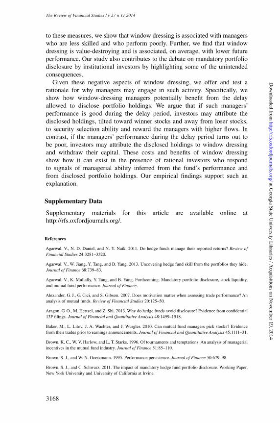
[18:05 9/10/2014 RFS-hhu045.tex] Page: 3168 3133–3170


to these measures, we show that window dressing is associated with managerswho are less skilled and who perform poorly. Further, we find that windowdressing is value-destroying and is associated, on average, with lower futureperformance. Our study also contributes to the debate on mandatory portfoliodisclosure by institutional investors by highlighting some of the unintendedconsequences.

Given these negative aspects of window dressing, we offer and test arationale for why managers may engage in such activity. Specifically, weshow how window-dressing managers potentially benefit from the delayallowed to disclose portfolio holdings. We argue that if such managers’performance is good during the delay period, investors may attribute thedisclosed holdings, tilted toward winner stocks and away from loser stocks,to security selection ability and reward the managers with higher flows. Incontrast, if the managers’ performance during the delay period turns out tobe poor, investors may attribute the disclosed holdings to window dressingand withdraw their capital. These costs and benefits of window dressingshow how it can exist in the presence of rational investors who respondto signals of managerial ability inferred from the fund’s performance andfrom disclosed portfolio holdings. Our empirical findings support such anexplanation.

Supplementary Data

Supplementary materials for this article are available online athttp://rfs.oxfordjournals.org/.

References

Agarwal, V., N. D. Daniel, and N. Y. Naik. 2011. Do hedge funds manage their reported returns? Review ofFinancial Studies 24:3281–3320.

Agarwal, V., W. Jiang, Y. Tang, and B. Yang. 2013. Uncovering hedge fund skill from the portfolios they hide.Journal of Finance 68:739–83.

Agarwal, V., K. Mullally, Y. Tang, and B. Yang. Forthcoming. Mandatory portfolio disclosure, stock liquidity,and mutual fund performance. Journal of Finance.

Alexander, G. J., G. Cici, and S. Gibson. 2007. Does motivation matter when assessing trade performance? Ananalysis of mutual funds. Review of Financial Studies 20:125–50.

Aragon, G. O., M. Hertzel, and Z. Shi. 2013. Why do hedge funds avoid disclosure? Evidence from confidential13F filings. Journal of Financial and Quantitative Analysis 48:1499–1518.

Baker, M., L. Litov, J. A. Wachter, and J. Wurgler. 2010. Can mutual fund managers pick stocks? Evidencefrom their trades prior to earnings announcements. Journal of Financial and Quantitative Analysis 45:1111–31.

Brown, K. C., W. V. Harlow, and L. T. Starks. 1996. Of tournaments and temptations: An analysis of managerialincentives in the mutual fund industry. Journal of Finance 51:85–110.

Brown, S. J., and W. N. Goetzmann. 1995. Performance persistence. Journal of Finance 50:679–98.

Brown, S. J., and C. Schwarz. 2011. The impact of mandatory hedge fund portfolio disclosure. Working Paper,New York University and University of California at Irvine.

3168

at Georgia State U




Dow

nloaded from



[18:05 9/10/2014 RFS-hhu045.tex] Page: 3169 3133–3170


Carhart, M. M. 1997. On persistence in mutual fund performance. Journal of Finance 52:57–82.

Carhart, M. M., R. Kaniel, D. K. Musto, and A. V. Reed. 2002. Leaning for the tape: Evidence of gaming behaviorin equity mutual funds. Journal of Finance 58:661–93.

Chen, H., N. Jegadeesh, and R. Wermers. 2000. The value of active mutual fund management: An examinationof the stockholdings and trades of fund managers. Journal of Financial and Quantitative Analysis 35:343–68.

Chen, H., and V. Singal. 2004.All things considered, taxes drive the January effect. Journal of Financial Research27:351–72.

Chevalier, J., and G. Ellison. 1997. Risk taking by mutual funds as a response to incentives. Journal of PoliticalEconomy 105:1167–1200.

Cohen, R. B., J. D. Coval, and L. Pastor. 2005. Judging fund managers by the company they keep. Journal ofFinance 60:1057–94.

Cremers, K. J. M., and A. Petajisto. 2009. How active is your fund manager? A new measure that predictsperformance. Review of Financial Studies 22:3329–65.

Daniel, K., M. Grinblatt, S. Titman, and R. Wermers. 1997. Measuring mutual fund performance withcharacteristic-based benchmarks. Journal of Finance 52:1035–58.

Frank, M. M., J. M. Poterba, D. A. Shackelford, and J. B. Shoven. 2004. Copycat funds: Information disclosureregulation and the returns to active management in the mutual fund industry. Journal of Law and Economics47:515–41.

Ge, W., and L. Zheng. 2006. The frequency of mutual fund portfolio disclosure. Working Paper, University ofWashington and University of California at Irvine.

Gompers, P. A., and A. Metrick. 2001. Institutional investors and equity prices. Quarterly Journal of Economics116:229–59.

Grinblatt, M., and S. Titman. 1989. Mutual fund performance:An analysis of quarterly portfolio holdings. Journalof Business 62:394–416.

———. 1993. Performance measurement without benchmarks: An examination of mutual fund returns. Journalof Business 66:47–68.

Grinblatt, M., S. Titman, and R. Wermers. 1995. Momentum investment strategies, portfolio performance, andherding: A study of mutual fund behavior. American Economic Review 85:1088–1105.

Haugen, R. A., and J. Lakonishok. 1988. The incredible January effect: The stock market’s unsolved mystery.Homewood, Illinois: Dow Jones-Irwin.

He, J., L. Ng, and Q. Wang. 2004. Quarterly trading patterns of financial institutions. Journal of Business77:493–509.

Hu, G., R. D. McLean, J. Pontiff, and Q. Wang. 2014. The year-end trading activities of institutional investors:Evidence from daily trades. Review of Financial Studies 27:1593–1614.

Hu, P., J. R. Kale, M. Pagani, and A. Subramanian. 2011. Fund flows, performance, managerial career concerns,and risk-taking. Management Science 57:628–46.

Huang, J., K. D. Wei, and H. Yan. 2007. Participation costs and the sensitivity of fund flows to past performance.Journal of Finance 62:1273–1311.

Huang, L., and J. R. Kale. 2013. Product market linkages, manager quality, and mutual fund performance. Reviewof Finance 17:1895–1946.

Ippolito, R. A. 1992. Consumer reaction to measures of poor quality: Evidence from the mutual fund industry.Journal of Law and Economics 35:45–70.

Jegadeesh, N., and S. Titman. 1993. Returns to buying winners and selling losers: Implications for stock marketefficiency. Journal of Finance 48:65–91.

3169

at Georgia State U




Dow

nloaded from


[18:05 9/10/2014 RFS-hhu045.tex] Page: 3170 3133–3170


Jiang, G. J., T. Yao, and T. Yu. 2007. Do mutual funds time the market? Evidence from portfolio holdings. Journalof Financial Economics 86:724–58.

Kacperczyk, M., and A. Seru. 2007. Fund manager use of public information: New evidence on managerial skills.Journal of Finance 62:485–528.

Kacperczyk, M., C. Sialm, and L. Zheng. 2005. On the industry concentration of actively managed equity funds.Journal of Finance 60:1983–2012.

———. 2008. Unobserved actions of mutual funds. Review of Financial Studies 21:2379–2416.

Khorana, A. 1996. Top management turnover: An empirical investigation of mutual fund managers. Journal ofFinancial Economics 40:403–27.

Lakonishok, J.,A. Shleifer, R. Thaler, and R. Vishny. 1991. Window dressing by pension fund managers. AmericanEconomic Review 81:227–31.

Meier, I., and E. Schaumburg. 2004. Do funds window dress? Evidence for U.S. domestic equity mutual funds.Working Paper, HEC Montreal and Kellogg School of Management.

Morey, M. R., and E. O’Neal. 2006. Window dressing in bond mutual funds. Journal of Financial Research29:325–47.

Moskowitz, T. J. 2000. Mutual fund performance: An empirical decomposition into stock-picking talent, style,transaction costs, and expenses: Discussion. Journal of Finance 55:1695–1703.

Musto, D. K. 1997. Portfolio disclosure and year-end price shift. Journal of Finance 52:1563–88.

———. 1999. Investment decisions depend on portfolio disclosures. Journal of Finance 54:935–52.

Ng, L., and Q. Wang. 2004. Institutional trading and the turn-of-the-year effect. Journal of Financial Economics74:343–66.

Poterba, J. M., and S. J. Weisbenner. 2001. Capital gains tax rules, tax-loss trading, and turn-of-the-year returns.Journal of Finance 56:353–68.

Ritter, J. R., and N. Chopra. 1989. Portfolio rebalancing and the turn-of-the-year effect. Journal of Finance44:149–66.

Sias, R. W. 2007. Causes and seasonality of momentum profits. Financial Analysts Journal 63:48–54.

Sias, R. W., and L. T. Starks. 1997. Institutions and individuals at the turn-of-the-year. Journal of Finance52:1543–62.

Sias, R. W., L. T. Starks, and S. Titman. 2006. Changes in institutional ownership and stock returns: Assessmentand methodology. Journal of Business 79:2869–2910.

Sirri, E. R., and P. Tufano. 1998. Costly search and mutual fund flows. Journal of Finance 53:1589–1622.

Solomon, D. H., E. F. Soltes, and D. Sosyura. 2014. Winners in the spotlight: Media coverage of fund holdingsas a driver of flows. Journal of Financial Economics 113:53–72.

Starks, L. T., L. Yong, and L. Zheng. 2006. Tax-loss selling and the January effect: Evidence from municipalbond closed-end funds. Journal of Finance 61:3049–67.

Verbeek, M., and Y. Wang. 2013. Better than the original? The relative success of copycat funds. Journal ofBanking & Finance 37:3454–71.

Wermers, R. 1999. Mutual fund herding and the impact on stock prices. Journal of Finance 54:581–622.

———. 2000. Mutual fund performance:An empirical decomposition into stock-picking talent, style, transactioncosts, and expenses. Journal of Finance 55:1655–95.

———. 2001. The potential effects of more frequent portfolio disclosure on mutual performance. InvestmentCompany Institute Perspective 7:1–12.

3170

at Georgia State U




Dow

nloaded from


Documents

Window Dressing in Mutual Funds - Georgia State Universityfncvaa/Windowdressing RFS_FINAL.pdf · Wang,andChongXiaofortheirhelpfulcommentsandconstructivesuggestions ... (Carhart et