Embed Size (px)
Citation preview
3.3 Optimizing Functions of Several Variables3.4 Lagrange Multipliers
Prof. Tesler
Math 20CWinter 2018
Prof. Tesler 3.3–3.4 Optimization Math 20C / Winter 2018 1 / 54
Optimizing y = f (x)
In Math 20A, we found the minimum and maximum of y = f (x) byusing derivatives.
First derivative:Solve for points where f ′(x) = 0.Each such point is called a critical point .
Second derivative:For each critical point x = a, check the sign of f ′′(a):
f ′′(a) > 0: The value y = f (a) is a local minimum.f ′′(a) < 0: The value y = f (a) is a local maximum.f ′′(a) = 0: The test is inconclusive.
Also may need to check points where f (x) is defined but thederivatives aren’t, as well as boundary points.
We will generalize this to functions z = f (x, y).
Prof. Tesler 3.3–3.4 Optimization Math 20C / Winter 2018 2 / 54
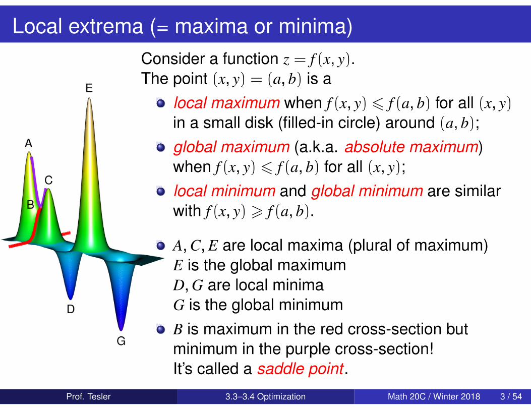
Local extrema (= maxima or minima)Consider a function z = f (x, y).The point (x, y) = (a, b) is a
local maximum when f (x, y) 6 f (a, b) for all (x, y)in a small disk (filled-in circle) around (a, b);global maximum (a.k.a. absolute maximum)when f (x, y) 6 f (a, b) for all (x, y);local minimum and global minimum are similarwith f (x, y) > f (a, b).
A, C, E are local maxima (plural of maximum)E is the global maximumD, G are local minimaG is the global minimumB is maximum in the red cross-section butminimum in the purple cross-section!It’s called a saddle point .
Prof. Tesler 3.3–3.4 Optimization Math 20C / Winter 2018 3 / 54
Critical points on a contour map
−3 −2 −1 0 1 2 3
−10
12
34
1
1
●P ●Q
●R
●
S
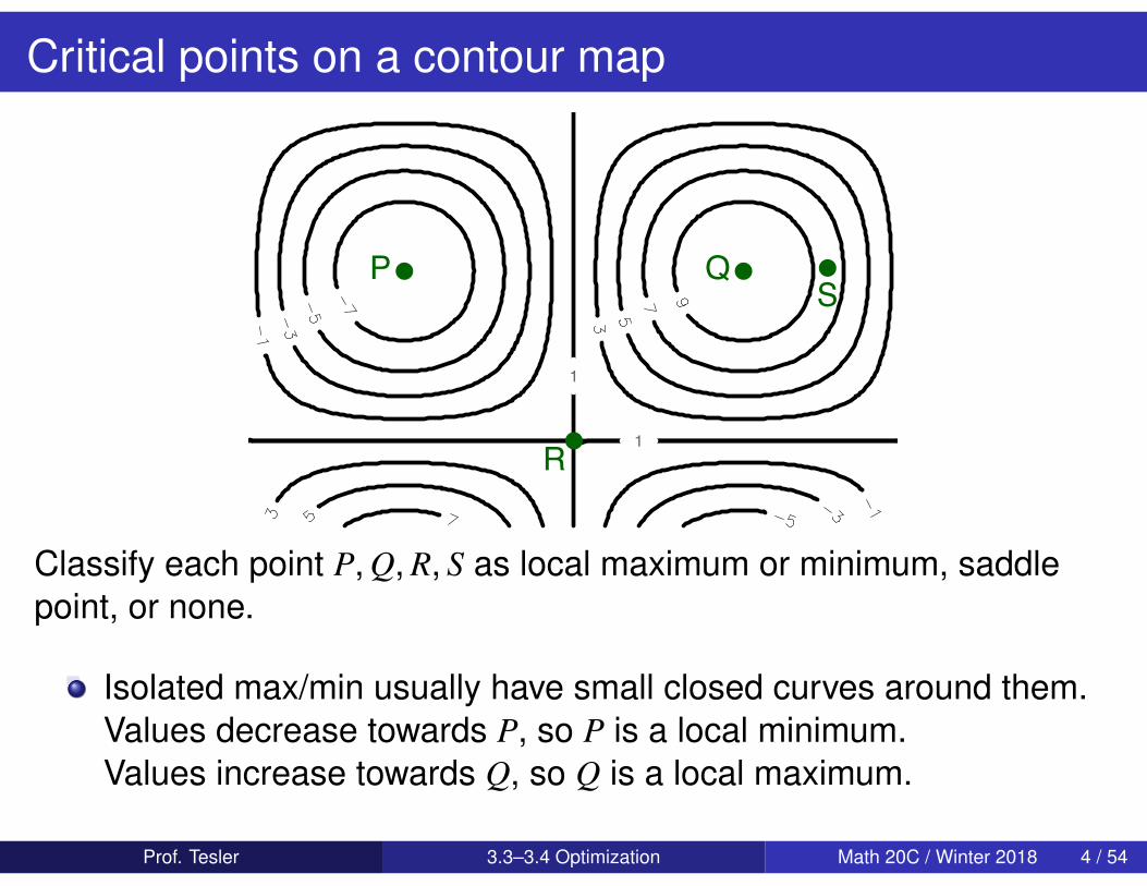
Classify each point P, Q, R, S as local maximum or minimum, saddlepoint, or none.
Isolated max/min usually have small closed curves around them.Values decrease towards P, so P is a local minimum.Values increase towards Q, so Q is a local maximum.
Prof. Tesler 3.3–3.4 Optimization Math 20C / Winter 2018 4 / 54
Critical points on a contour map
−3 −2 −1 0 1 2 3
−10
12
34
1
1
●P ●Q
●R
●
S
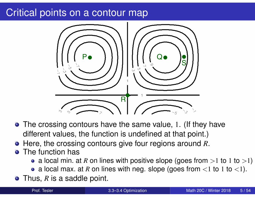
The crossing contours have the same value, 1. (If they havedifferent values, the function is undefined at that point.)Here, the crossing contours give four regions around R.The function has
a local min. at R on lines with positive slope (goes from >1 to 1 to >1)a local max. at R on lines with neg. slope (goes from <1 to 1 to <1).
Thus, R is a saddle point.Prof. Tesler 3.3–3.4 Optimization Math 20C / Winter 2018 5 / 54
Critical points on a contour map
−3 −2 −1 0 1 2 3
−10
12
34
1
1
●P ●Q
●R
●
S
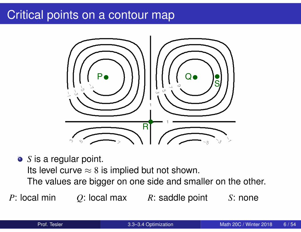
S is a regular point.Its level curve ≈ 8 is implied but not shown.The values are bigger on one side and smaller on the other.
P: local min Q: local max R: saddle point S: none
Prof. Tesler 3.3–3.4 Optimization Math 20C / Winter 2018 6 / 54
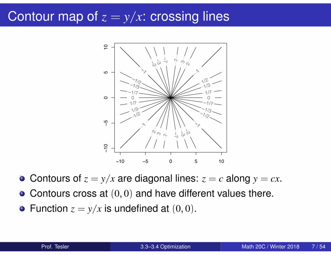
Contour map of z = y/x: crossing lines
−10 −5 0 5 10
−10
−50
51000
1
1 −1
−1 1
1 −1
−1
2
2−2
−2
1/2
1/2−1/2
−1/2
3
3
−3
−3
1/3
1/3 −1/3
−1/3
7
7
−7
−7
1/7
1/7 −1/7
−1/7
Contours of z = y/x are diagonal lines: z = c along y = cx.Contours cross at (0, 0) and have different values there.Function z = y/x is undefined at (0, 0).
Prof. Tesler 3.3–3.4 Optimization Math 20C / Winter 2018 7 / 54
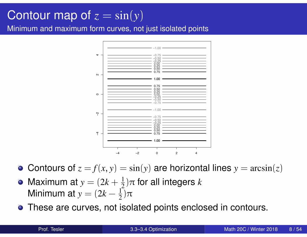
Contour map of z = sin(y)Minimum and maximum form curves, not just isolated points
−4 −2 0 2 4
−4−2
02
4
−1.00−1.00
−1.00−1.00
−0.75
−0.75
−0.75
−0.50
−0.50
−0.50
−0.25
−0.25
−0.25
0.00
0.00
0.00
0.25
0.25
0.25
0.50
0.50
0.50
0.75
0.75
0.75
1.001.00
1.001.00
Contours of z = f (x, y) = sin(y) are horizontal lines y = arcsin(z)
Maximum at y = (2k + 12)π for all integers k
Minimum at y = (2k − 12)π
These are curves, not isolated points enclosed in contours.
Prof. Tesler 3.3–3.4 Optimization Math 20C / Winter 2018 8 / 54
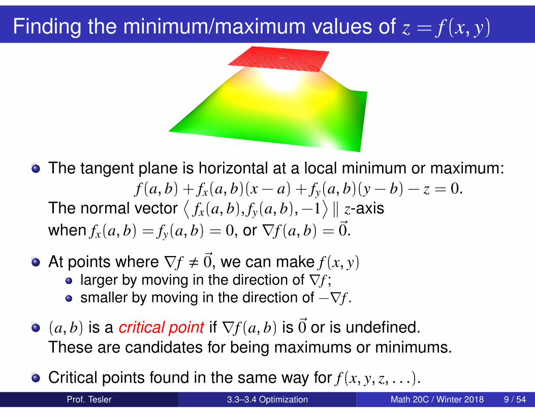
Finding the minimum/maximum values of z = f (x, y)
The tangent plane is horizontal at a local minimum or maximum:f (a, b) + fx(a, b)(x − a) + fy(a, b)(y − b) − z = 0.
The normal vector⟨
fx(a, b), fy(a, b),−1⟩‖ z-axis
when fx(a, b) = fy(a, b) = 0, or ∇f (a, b) = ~0.
At points where ∇f , ~0, we can make f (x, y)larger by moving in the direction of ∇f ;smaller by moving in the direction of −∇f .
(a, b) is a critical point if ∇f (a, b) is ~0 or is undefined.These are candidates for being maximums or minimums.
Critical points found in the same way for f (x, y, z, . . .).Prof. Tesler 3.3–3.4 Optimization Math 20C / Winter 2018 9 / 54
Critical points
Let f (x, y)= x2 − 2x + y2 − 4y + 15∇f = 〈2x − 2, 2y − 4〉
∇f = ~0 at x = 1, y = 2, so (1, 2) is a critical point.
Use (x − 1)2 = x2 − 2x + 1(y − 2)2 = y2 − 4y + 4
f (x, y)= (x − 1)2 + (y − 2)2 + 10
We “completed the squares”: x2 − ax = (x − a2)
2 − ( a2)
2
f (x, y) > 10 everywhere, with global minimum 10 at (x, y) = (1, 2).
Prof. Tesler 3.3–3.4 Optimization Math 20C / Winter 2018 10 / 54
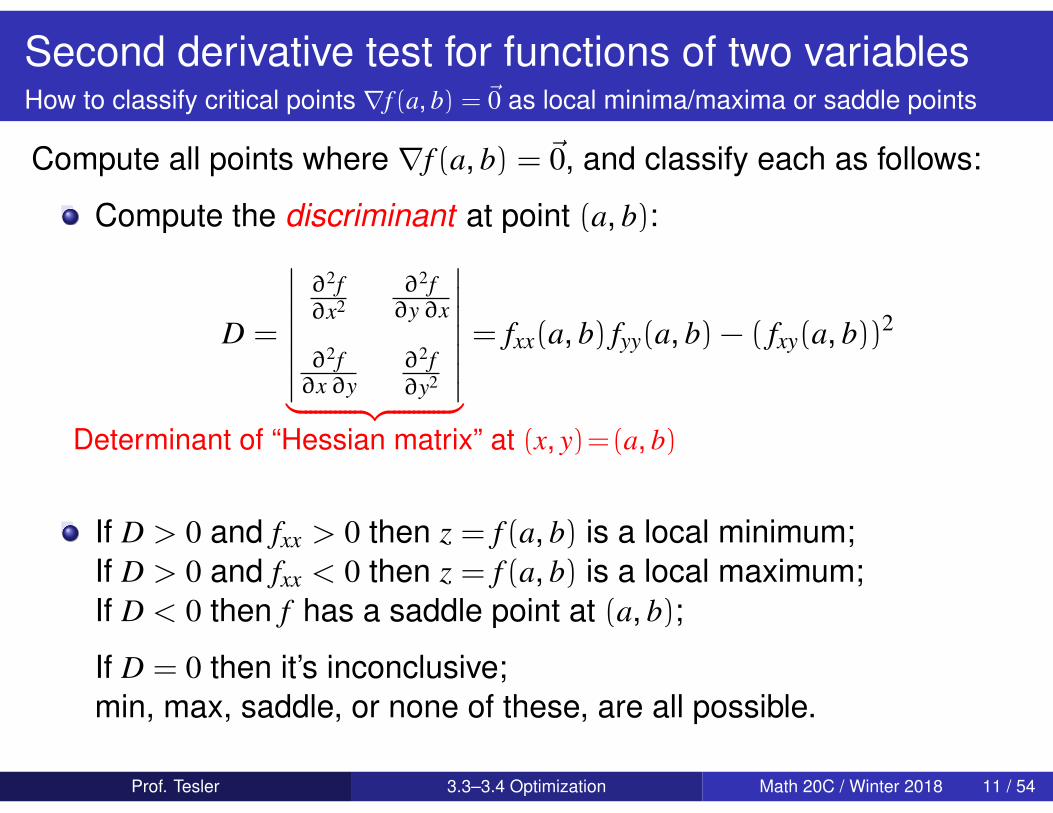
Second derivative test for functions of two variablesHow to classify critical points ∇f (a, b) = ~0 as local minima/maxima or saddle points
Compute all points where ∇f (a, b) = ~0, and classify each as follows:
Compute the discriminant at point (a, b):
D =
∣∣∣∣∣∣∣∂2f∂x2
∂2f∂y∂x
∂2f∂x∂y
∂2f∂y2
∣∣∣∣∣∣∣︸ ︷︷ ︸Determinant of “Hessian matrix” at (x, y)=(a, b)
= fxx(a, b) fyy(a, b) − ( fxy(a, b))2
If D > 0 and fxx > 0 then z = f (a, b) is a local minimum;If D > 0 and fxx < 0 then z = f (a, b) is a local maximum;If D < 0 then f has a saddle point at (a, b);
If D = 0 then it’s inconclusive;min, max, saddle, or none of these, are all possible.
Prof. Tesler 3.3–3.4 Optimization Math 20C / Winter 2018 11 / 54
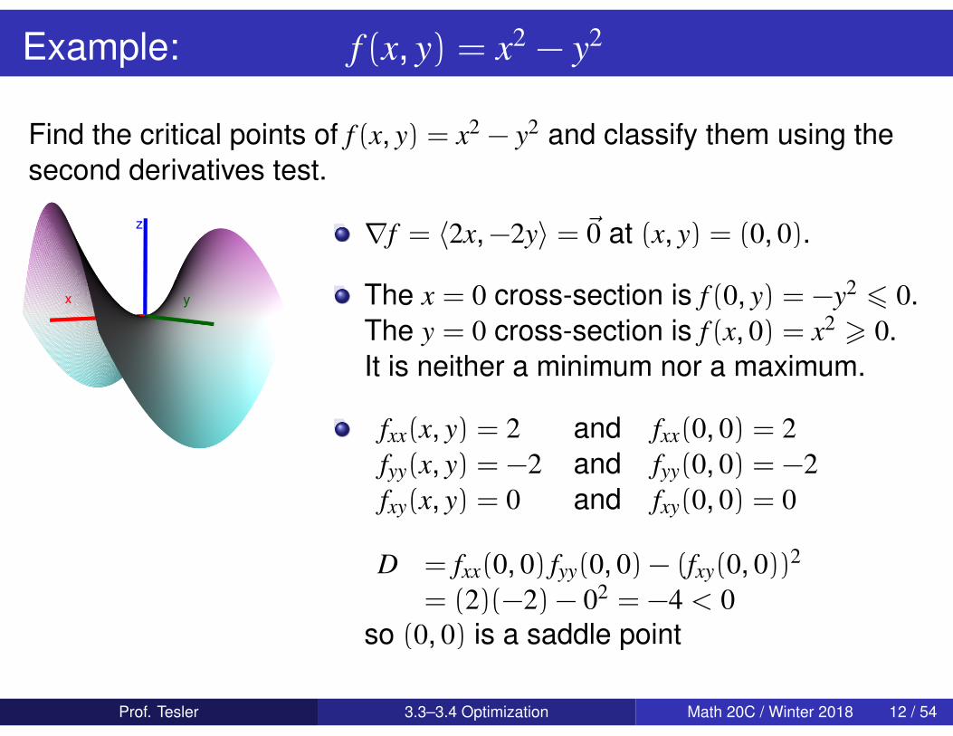
Example: f (x, y) = x2 − y2
Find the critical points of f (x, y) = x2 − y2 and classify them using thesecond derivatives test.
∇f = 〈2x,−2y〉 = ~0 at (x, y) = (0, 0).
The x = 0 cross-section is f (0, y) = −y2 6 0.The y = 0 cross-section is f (x, 0) = x2 > 0.It is neither a minimum nor a maximum.
fxx(x, y) = 2 and fxx(0, 0) = 2fyy(x, y) = −2 and fyy(0, 0) = −2fxy(x, y) = 0 and fxy(0, 0) = 0
D = fxx(0, 0) fyy(0, 0) − (fxy(0, 0))2
= (2)(−2) − 02 = −4 < 0so (0, 0) is a saddle point
Prof. Tesler 3.3–3.4 Optimization Math 20C / Winter 2018 12 / 54
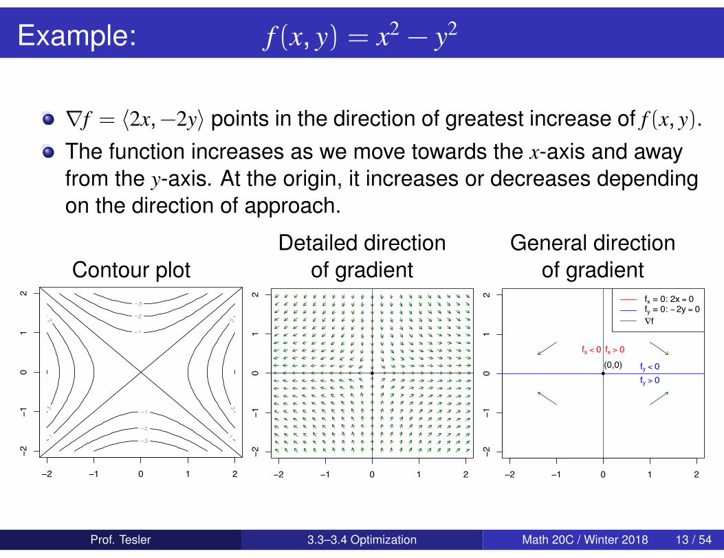
Example: f (x, y) = x2 − y2
∇f = 〈2x,−2y〉 points in the direction of greatest increase of f (x, y).The function increases as we move towards the x-axis and awayfrom the y-axis. At the origin, it increases or decreases dependingon the direction of approach.
Detailed direction General directionContour plot of gradient of gradient
−2 −1 0 1 2
−2−1
01
2
−2 −1 0 1 2
−2−1
01
2
!
−2 −1 0 1 2−2
−10
12
!
(0,0)fx > 0fx < 0
fy < 0fy > 0
fx = 0: 2x = 0fy = 0: !2y = 0"f
Prof. Tesler 3.3–3.4 Optimization Math 20C / Winter 2018 13 / 54
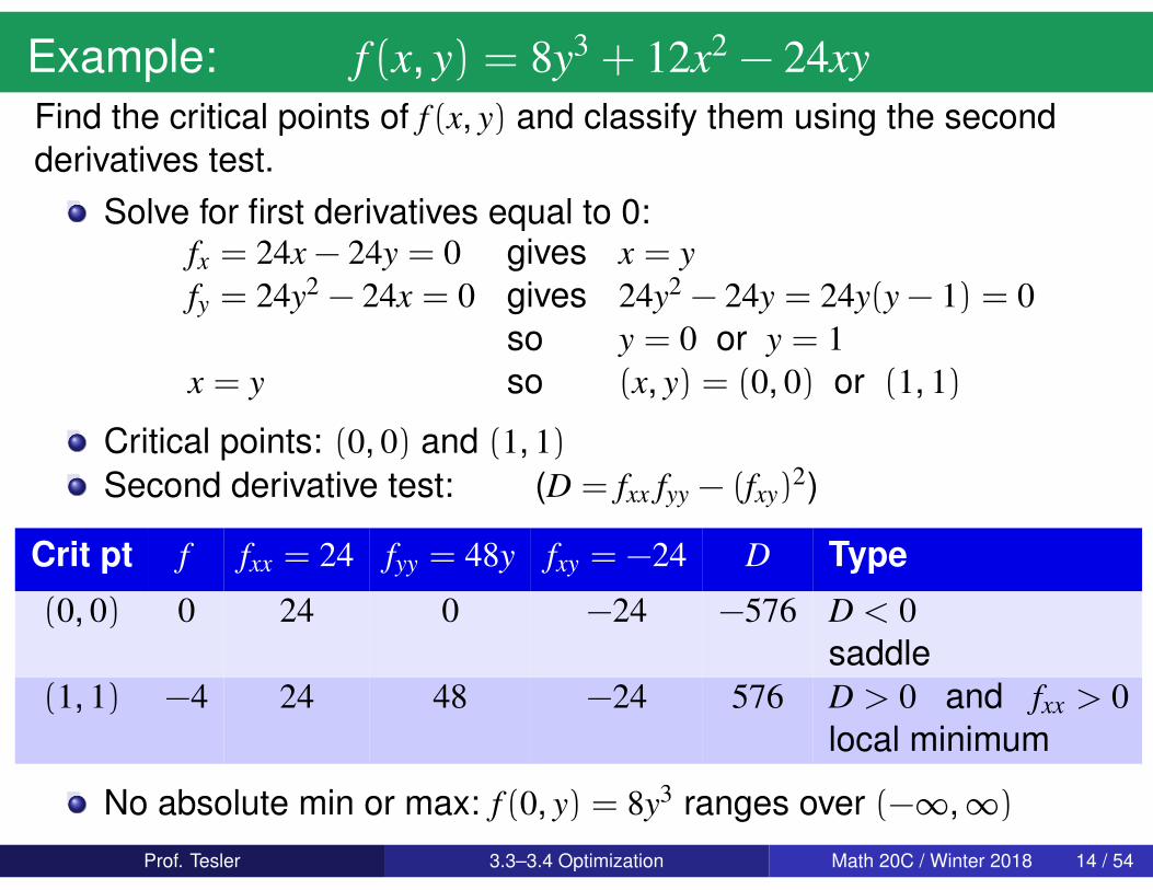
Example: f (x, y) = 8y3 + 12x2 − 24xyFind the critical points of f (x, y) and classify them using the secondderivatives test.
Solve for first derivatives equal to 0:fx = 24x − 24y = 0 gives x = yfy = 24y2 − 24x = 0 gives 24y2 − 24y = 24y(y − 1) = 0
so y = 0 or y = 1x = y so (x, y) = (0, 0) or (1, 1)
Critical points: (0, 0) and (1, 1)Second derivative test: (D = fxx fyy − (fxy)
2)
Crit pt f fxx = 24 fyy = 48y fxy = −24 D Type
(0, 0) 0 24 0 −24 −576 D < 0saddle
(1, 1) −4 24 48 −24 576 D > 0 and fxx > 0local minimum
No absolute min or max: f (0, y) = 8y3 ranges over (−∞,∞)
Prof. Tesler 3.3–3.4 Optimization Math 20C / Winter 2018 14 / 54
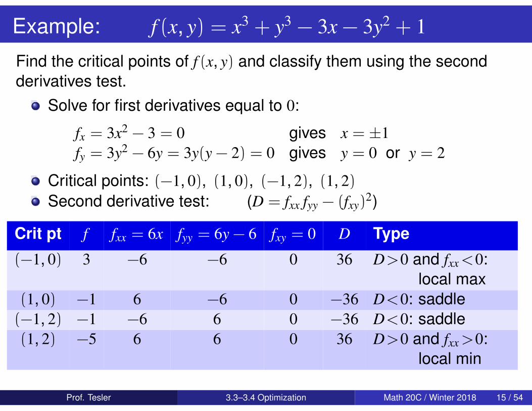
Example: f (x, y) = x3 + y3 − 3x − 3y2 + 1
Find the critical points of f (x, y) and classify them using the secondderivatives test.
Solve for first derivatives equal to 0:
fx = 3x2 − 3 = 0 gives x = ±1fy = 3y2 − 6y = 3y(y − 2) = 0 gives y = 0 or y = 2
Critical points: (−1, 0), (1, 0), (−1, 2), (1, 2)Second derivative test: (D = fxx fyy − (fxy)
2)
Crit pt f fxx = 6x fyy = 6y − 6 fxy = 0 D Type
(−1, 0) 3 −6 −6 0 36 D>0 and fxx<0:local max
(1, 0) −1 6 −6 0 −36 D<0: saddle(−1, 2) −1 −6 6 0 −36 D<0: saddle(1, 2) −5 6 6 0 36 D>0 and fxx>0:
local min
Prof. Tesler 3.3–3.4 Optimization Math 20C / Winter 2018 15 / 54
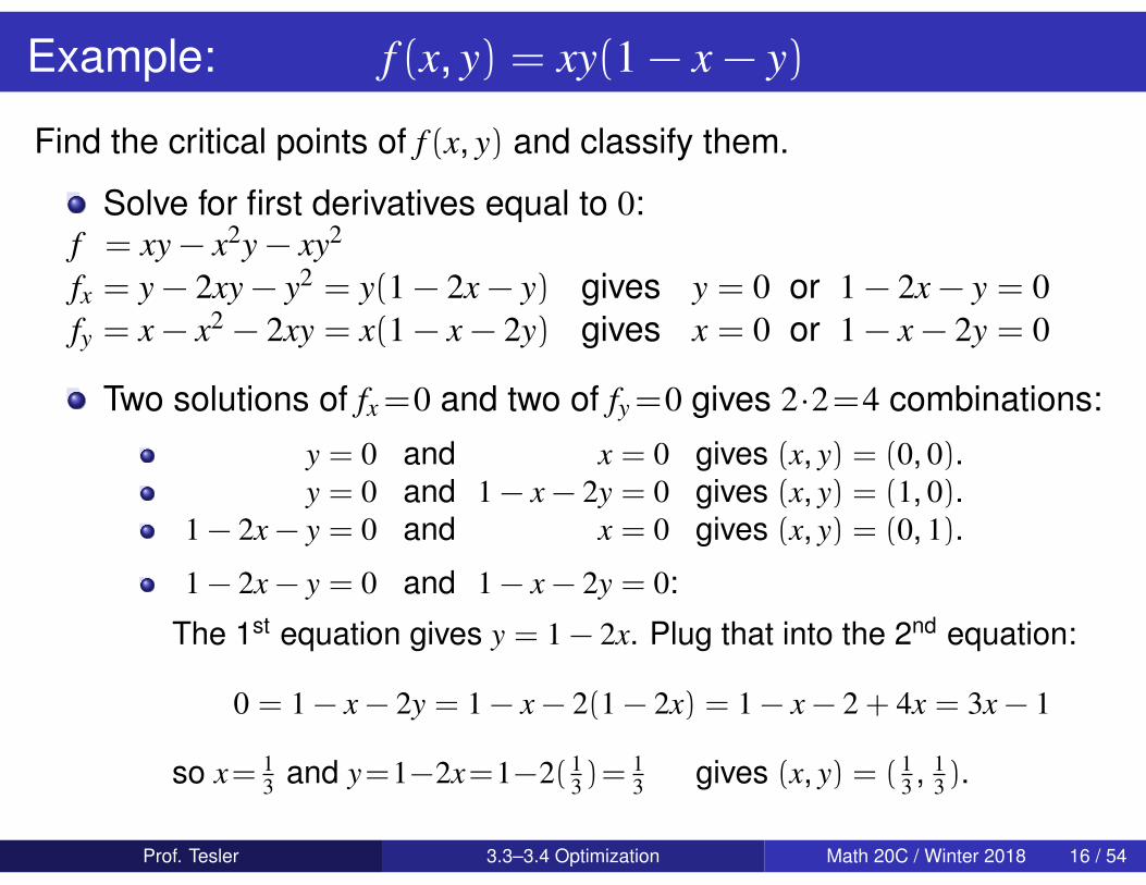
Example: f (x, y) = xy(1 − x − y)
Find the critical points of f (x, y) and classify them.
Solve for first derivatives equal to 0:f = xy − x2y − xy2
fx = y − 2xy − y2 = y(1 − 2x − y) gives y = 0 or 1 − 2x − y = 0fy = x − x2 − 2xy = x(1 − x − 2y) gives x = 0 or 1 − x − 2y = 0
Two solutions of fx=0 and two of fy=0 gives 2·2=4 combinations:
y = 0 and x = 0 gives (x, y) = (0, 0).y = 0 and 1 − x − 2y = 0 gives (x, y) = (1, 0).
1 − 2x − y = 0 and x = 0 gives (x, y) = (0, 1).
1 − 2x − y = 0 and 1 − x − 2y = 0:
The 1st equation gives y = 1 − 2x. Plug that into the 2nd equation:
0 = 1 − x − 2y = 1 − x − 2(1 − 2x) = 1 − x − 2 + 4x = 3x − 1
so x= 13 and y=1−2x=1−2( 1
3 )=13 gives (x, y) = ( 1
3 , 13 ).
Prof. Tesler 3.3–3.4 Optimization Math 20C / Winter 2018 16 / 54
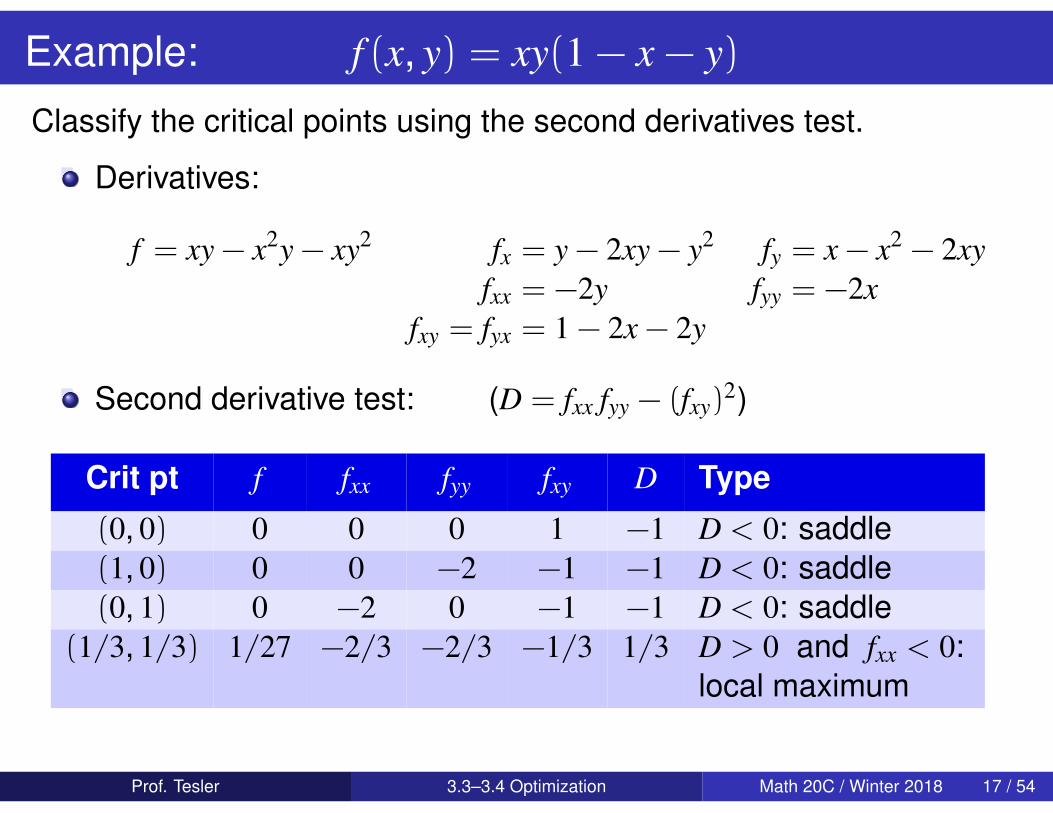
Example: f (x, y) = xy(1 − x − y)
Classify the critical points using the second derivatives test.
Derivatives:
f = xy − x2y − xy2 fx = y − 2xy − y2 fy = x − x2 − 2xyfxx = −2y fyy = −2x
fxy = fyx = 1 − 2x − 2y
Second derivative test: (D = fxx fyy − (fxy)2)
Crit pt f fxx fyy fxy D Type
(0, 0) 0 0 0 1 −1 D < 0: saddle(1, 0) 0 0 −2 −1 −1 D < 0: saddle(0, 1) 0 −2 0 −1 −1 D < 0: saddle
(1/3, 1/3) 1/27 −2/3 −2/3 −1/3 1/3 D > 0 and fxx < 0:local maximum
Prof. Tesler 3.3–3.4 Optimization Math 20C / Winter 2018 17 / 54
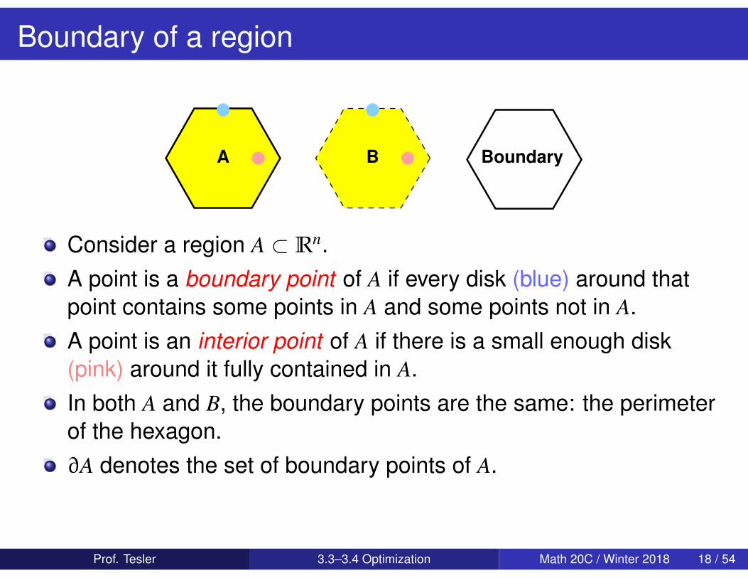
Boundary of a region
BoundaryA B
Consider a region A ⊂ Rn.A point is a boundary point of A if every disk (blue) around thatpoint contains some points in A and some points not in A.A point is an interior point of A if there is a small enough disk(pink) around it fully contained in A.In both A and B, the boundary points are the same: the perimeterof the hexagon.∂A denotes the set of boundary points of A.
Prof. Tesler 3.3–3.4 Optimization Math 20C / Winter 2018 18 / 54
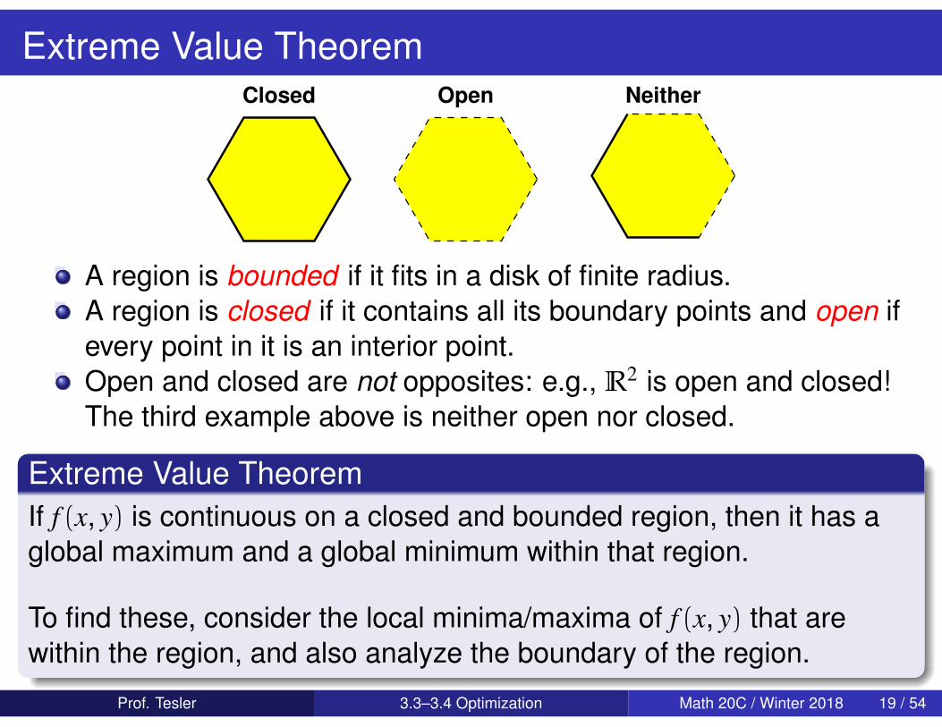
Extreme Value TheoremClosed Open Neither
A region is bounded if it fits in a disk of finite radius.A region is closed if it contains all its boundary points and open ifevery point in it is an interior point.Open and closed are not opposites: e.g., R2 is open and closed!The third example above is neither open nor closed.
Extreme Value TheoremIf f (x, y) is continuous on a closed and bounded region, then it has aglobal maximum and a global minimum within that region.
To find these, consider the local minima/maxima of f (x, y) that arewithin the region, and also analyze the boundary of the region.
Prof. Tesler 3.3–3.4 Optimization Math 20C / Winter 2018 19 / 54
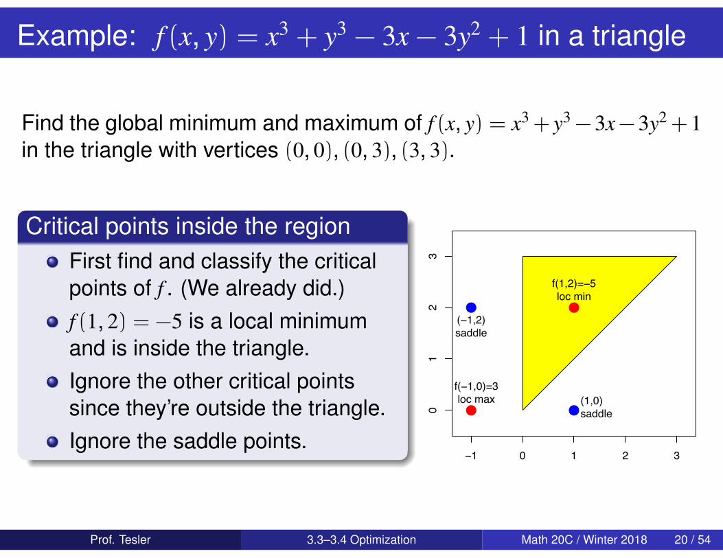
Example: f (x, y) = x3 + y3 − 3x − 3y2 + 1 in a triangle
Find the global minimum and maximum of f (x, y) = x3 + y3 − 3x− 3y2 + 1in the triangle with vertices (0, 0), (0, 3), (3, 3).
Critical points inside the regionFirst find and classify the criticalpoints of f . (We already did.)f (1, 2) = −5 is a local minimumand is inside the triangle.Ignore the other critical pointssince they’re outside the triangle.Ignore the saddle points.
−1 0 1 2 3
01
23
! !
! !
f(1,2)=−5loc min
(1,0)saddle
(−1,2)saddle
f(−1,0)=3loc max
Prof. Tesler 3.3–3.4 Optimization Math 20C / Winter 2018 20 / 54
Example: f (x, y) = x3 + y3 − 3x − 3y2 + 1 in a triangle
Find the global minimum and maximum of f (x, y) = x3 + y3 − 3x− 3y2 + 1in the triangle with vertices (0, 0), (0, 3), (3, 3).
−1 0 1 2 3 4
01
23
4
!
f(1,2)=−5loc min
!
! !
(0,0)
(0,3) (3,3)
Topy = 3
x ! 30 !
Diagonaly = x
x ! 30 !
Leftx = 0
y ! 30 !
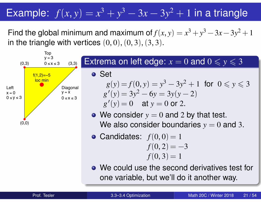
Extrema on left edge: x = 0 and 0 6 y 6 3Set
g(y)= f (0, y) = y3 − 3y2 + 1 for 0 6 y 6 3g ′(y)= 3y2 − 6y = 3y(y − 2)g ′(y)= 0 at y = 0 or 2.
We consider y = 0 and 2 by that test.We also consider boundaries y = 0 and 3.Candidates: f (0, 0)= 1
f (0, 2)= −3f (0, 3)= 1
We could use the second derivatives test forone variable, but we’ll do it another way.
Prof. Tesler 3.3–3.4 Optimization Math 20C / Winter 2018 21 / 54
Example: f (x, y) = x3 + y3 − 3x − 3y2 + 1 in a triangle
Find the global minimum and maximum of f (x, y) = x3 + y3 − 3x− 3y2 + 1in the triangle with vertices (0, 0), (0, 3), (3, 3).
−1 0 1 2 3 4
01
23
4
!
f(1,2)=−5loc min
!
! !
(0,0)
(0,3) (3,3)
Topy = 3
x ! 30 !
Diagonaly = x
x ! 30 !
Leftx = 0
y ! 30 !
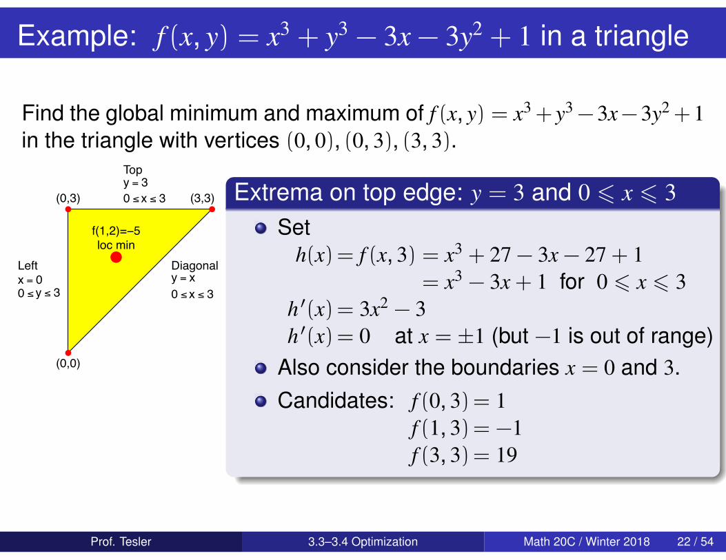
Extrema on top edge: y = 3 and 0 6 x 6 3Set
h(x)= f (x, 3) = x3 + 27 − 3x − 27 + 1= x3 − 3x + 1 for 0 6 x 6 3
h ′(x)= 3x2 − 3h ′(x)= 0 at x = ±1 (but −1 is out of range)
Also consider the boundaries x = 0 and 3.Candidates: f (0, 3)= 1
f (1, 3)= −1f (3, 3)= 19
Prof. Tesler 3.3–3.4 Optimization Math 20C / Winter 2018 22 / 54
Example: f (x, y) = x3 + y3 − 3x − 3y2 + 1 in a triangle
Find the global minimum and maximum of f (x, y) = x3 + y3 − 3x− 3y2 + 1in the triangle with vertices (0, 0), (0, 3), (3, 3).
−1 0 1 2 3 4
01
23
4
!
f(1,2)=−5loc min
!
! !
(0,0)
(0,3) (3,3)
Topy = 3
x ! 30 !
Diagonaly = x
x ! 30 !
Leftx = 0
y ! 30 !
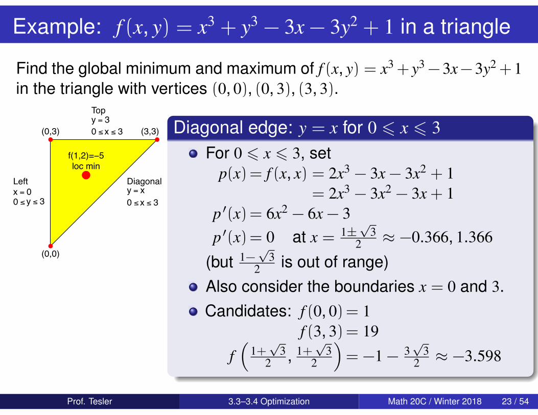
Diagonal edge: y = x for 0 6 x 6 3For 0 6 x 6 3, set
p(x)= f (x, x) = 2x3 − 3x − 3x2 + 1= 2x3 − 3x2 − 3x + 1
p ′(x)= 6x2 − 6x − 3p ′(x)= 0 at x = 1±
√3
2 ≈ −0.366, 1.366
(but 1−√
32 is out of range)
Also consider the boundaries x = 0 and 3.Candidates: f (0, 0)= 1
f (3, 3)= 19
f(
1+√
32 , 1+
√3
2
)= −1 − 3
√3
2 ≈ −3.598
Prof. Tesler 3.3–3.4 Optimization Math 20C / Winter 2018 23 / 54
Example: f (x, y) = x3 + y3 − 3x − 3y2 + 1 in a triangle
Find the global minimum and maximum of f (x, y) = x3 + y3 − 3x− 3y2 + 1in the triangle with vertices (0, 0), (0, 3), (3, 3).
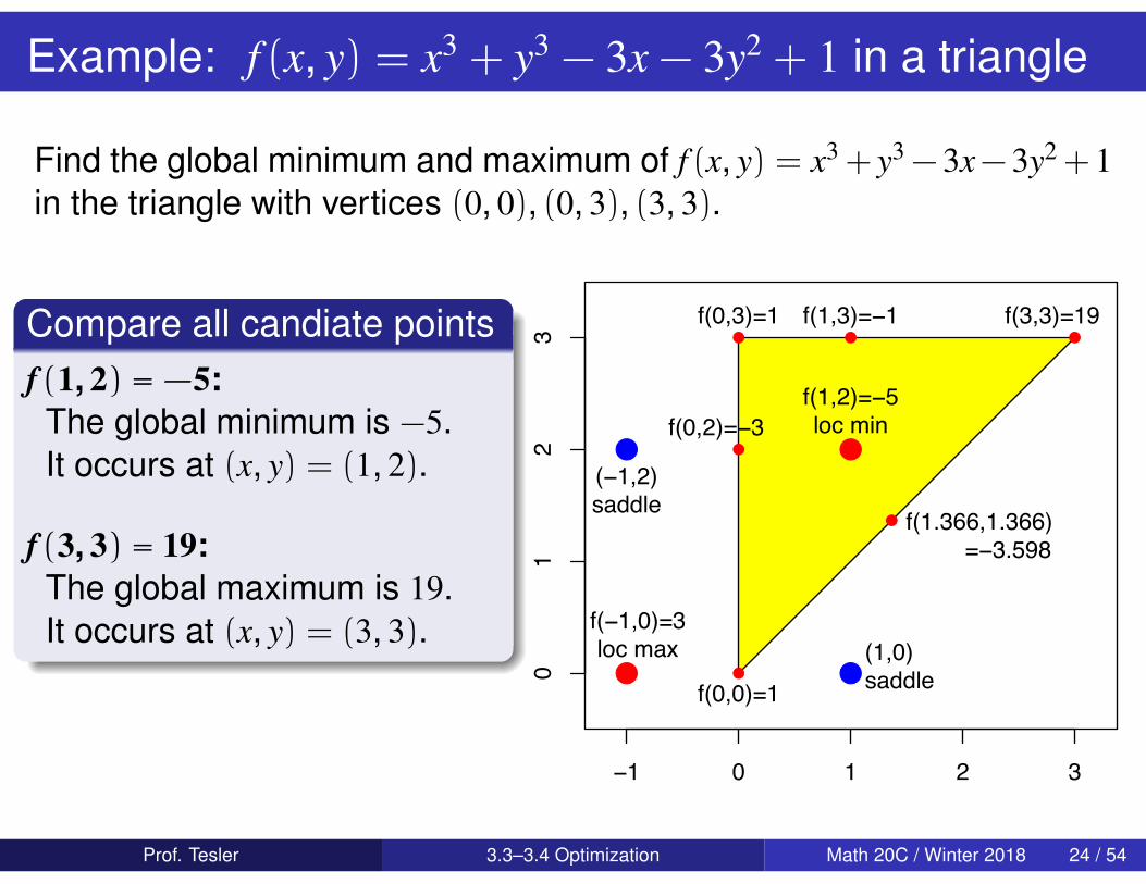
Compare all candiate pointsf(1, 2) = −5:The global minimum is −5.It occurs at (x, y) = (1, 2).
f(3, 3) = 19:The global maximum is 19.It occurs at (x, y) = (3, 3).
−1 0 1 2 3
01
23
! !
! !
f(1,2)=−5loc min
(1,0)saddle
(−1,2)saddle
f(−1,0)=3loc max
!
! !!
!
!
f(0,0)=1
f(0,2)=−3
f(0,3)=1 f(3,3)=19f(1,3)=−1
f(1.366,1.366) =−3.598
Prof. Tesler 3.3–3.4 Optimization Math 20C / Winter 2018 24 / 54
Extrema of f (x, y) = |xy|: ∇f isn’t defined everywhere
f=0
f(−1,−2)=2
f(−1,2)=2 f=0
f(1,−2)=2
f(1,2)=2
−2
2
1−1
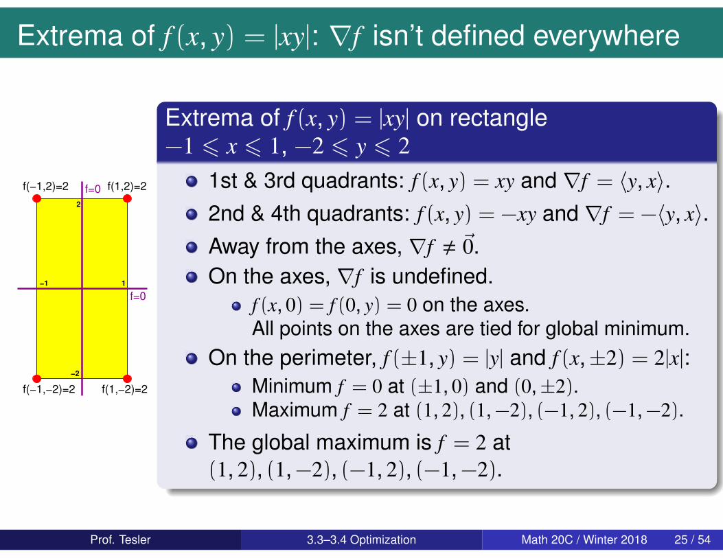
Extrema of f (x, y) = |xy| on rectangle−1 6 x 6 1, −2 6 y 6 2
1st & 3rd quadrants: f (x, y) = xy and ∇f = 〈y, x〉.2nd & 4th quadrants: f (x, y) = −xy and ∇f = −〈y, x〉.Away from the axes, ∇f , ~0.On the axes, ∇f is undefined.
f (x, 0) = f (0, y) = 0 on the axes.All points on the axes are tied for global minimum.
On the perimeter, f (±1, y) = |y| and f (x,±2) = 2|x|:Minimum f = 0 at (±1, 0) and (0,±2).Maximum f = 2 at (1, 2), (1,−2), (−1, 2), (−1,−2).
The global maximum is f = 2 at(1, 2), (1,−2), (−1, 2), (−1,−2).
Prof. Tesler 3.3–3.4 Optimization Math 20C / Winter 2018 25 / 54
Extrema of f (x, y) = |xy|: ∇f isn’t defined everywhere
f=0
f(−1,−2)=2
f(−1,2)=2 f=0
f(1,−2)=2
f(1,2)=2
−2
2
1−1
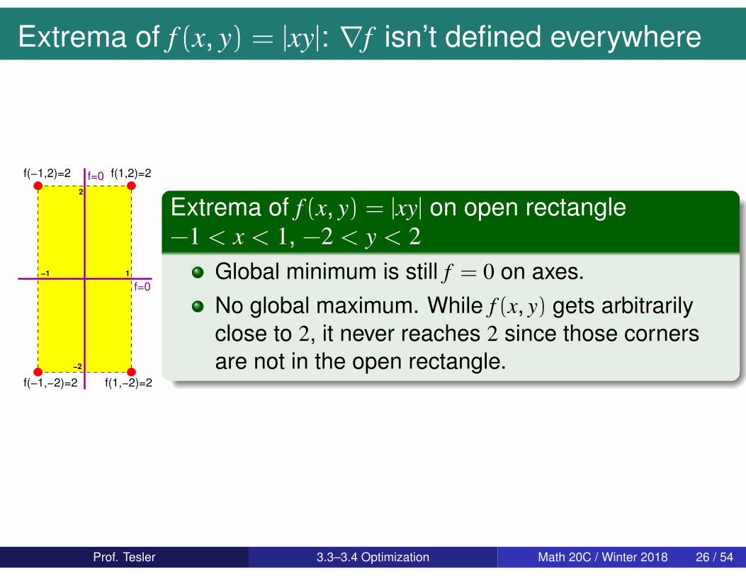
Extrema of f (x, y) = |xy| on open rectangle−1 < x < 1, −2 < y < 2
Global minimum is still f = 0 on axes.No global maximum. While f (x, y) gets arbitrarilyclose to 2, it never reaches 2 since those cornersare not in the open rectangle.
Prof. Tesler 3.3–3.4 Optimization Math 20C / Winter 2018 26 / 54
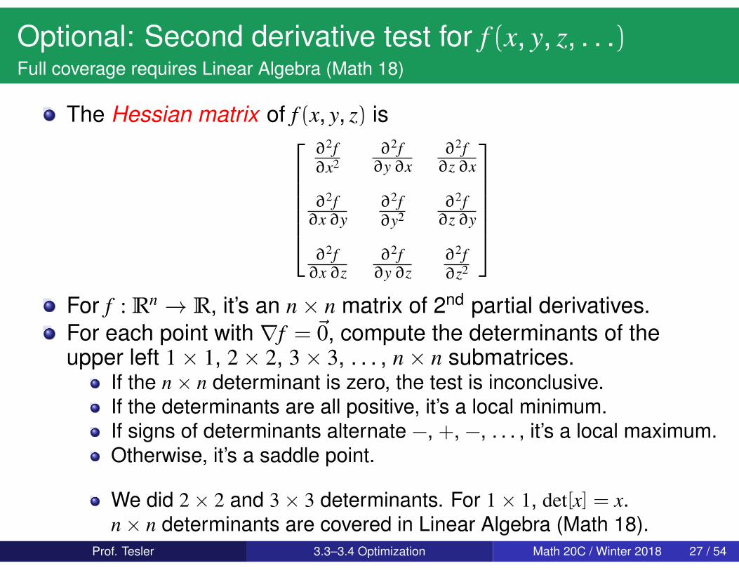
Optional: Second derivative test for f (x, y, z, . . .)Full coverage requires Linear Algebra (Math 18)
The Hessian matrix of f (x, y, z) is∂2f∂x2
∂2f∂y∂x
∂2f∂z∂x
∂2f∂x∂y
∂2f∂y2
∂2f∂z∂y
∂2f∂x∂z
∂2f∂y∂z
∂2f∂z2
For f : Rn → R, it’s an n× n matrix of 2nd partial derivatives.For each point with ∇f = ~0, compute the determinants of theupper left 1× 1, 2× 2, 3× 3, . . . , n× n submatrices.
If the n× n determinant is zero, the test is inconclusive.If the determinants are all positive, it’s a local minimum.If signs of determinants alternate −, +, −, . . . , it’s a local maximum.Otherwise, it’s a saddle point.
We did 2× 2 and 3× 3 determinants. For 1× 1, det[x] = x.n× n determinants are covered in Linear Algebra (Math 18).
Prof. Tesler 3.3–3.4 Optimization Math 20C / Winter 2018 27 / 54
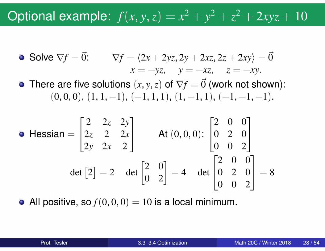
Optional example: f (x, y, z) = x2 + y2 + z2 + 2xyz + 10
Solve ∇f = ~0: ∇f = 〈2x + 2yz, 2y + 2xz, 2z + 2xy〉 = ~0x = −yz, y = −xz, z = −xy.
There are five solutions (x, y, z) of ∇f = ~0 (work not shown):(0, 0, 0), (1, 1,−1), (−1, 1, 1), (1,−1, 1), (−1,−1,−1).
Hessian =
2 2z 2y2z 2 2x2y 2x 2
At (0, 0, 0):
2 0 00 2 00 0 2
det[2]= 2 det
[2 00 2
]= 4 det
2 0 00 2 00 0 2
= 8
All positive, so f (0, 0, 0) = 10 is a local minimum.
Prof. Tesler 3.3–3.4 Optimization Math 20C / Winter 2018 28 / 54
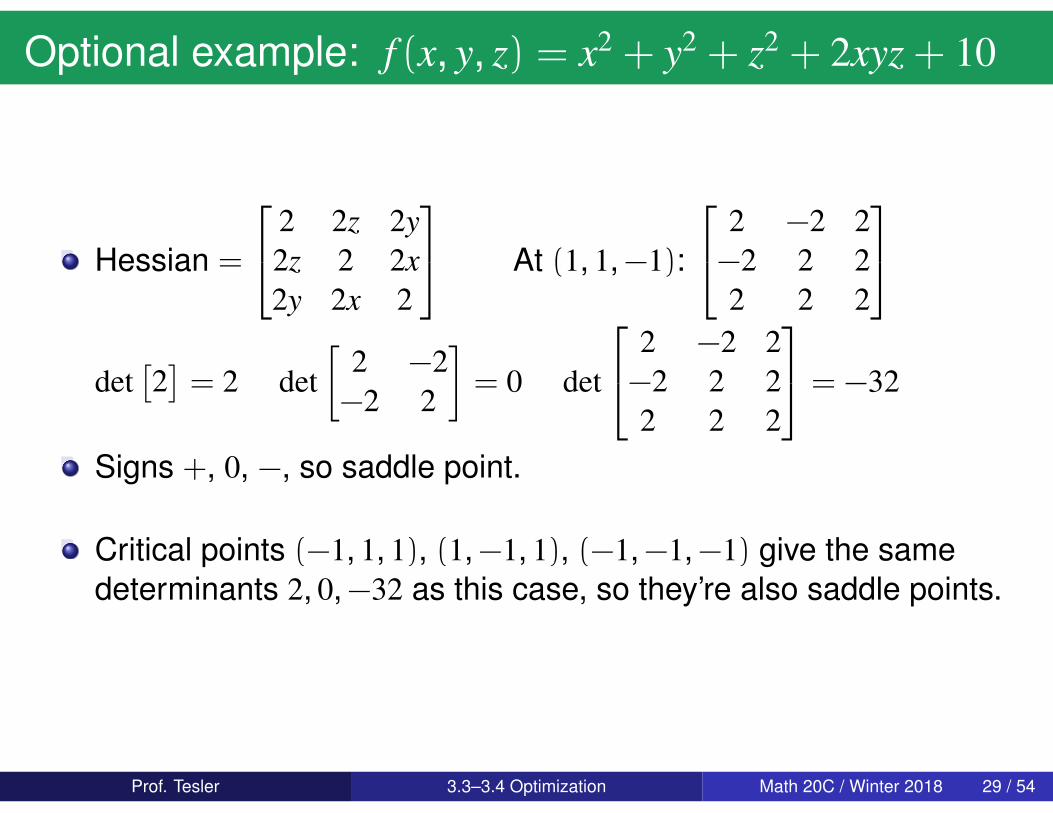
Optional example: f (x, y, z) = x2 + y2 + z2 + 2xyz + 10
Hessian =
2 2z 2y2z 2 2x2y 2x 2
At (1, 1,−1):
2 −2 2−2 2 22 2 2
det[2]= 2 det
[2 −2−2 2
]= 0 det
2 −2 2−2 2 22 2 2
= −32
Signs +, 0, −, so saddle point.
Critical points (−1, 1, 1), (1,−1, 1), (−1,−1,−1) give the samedeterminants 2, 0,−32 as this case, so they’re also saddle points.
Prof. Tesler 3.3–3.4 Optimization Math 20C / Winter 2018 29 / 54
Optimization with a constraint
−1.0 −0.5 0.0 0.5 1.0
−1.0
−0.5
0.0
0.5
1.0
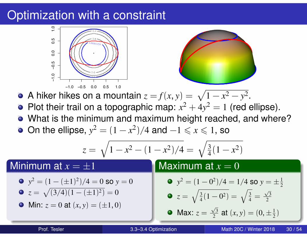
A hiker hikes on a mountain z = f (x, y) =√
1 − x2 − y2.Plot their trail on a topographic map: x2 + 4y2 = 1 (red ellipse).What is the minimum and maximum height reached, and where?On the ellipse, y2 = (1 − x2)/4 and −1 6 x 6 1, so
z =√
1 − x2 − (1 − x2)/4 =√
34(1 − x2)
Minimum at x = ±1y2 = (1 − (±1)2)/4 = 0 so y = 0z =
√(3/4)(1 − (±1)2) = 0
Min: z = 0 at (x, y) = (±1, 0)
Maximum at x = 0y2 = (1 − 02)/4 = 1/4 so y = ± 1
2
z =√
34 (1 − 02) =
√34 =
√3
2
Max: z =√
32 at (x, y) = (0,± 1
2 )
Prof. Tesler 3.3–3.4 Optimization Math 20C / Winter 2018 30 / 54
3.4. Lagrange Multipliers
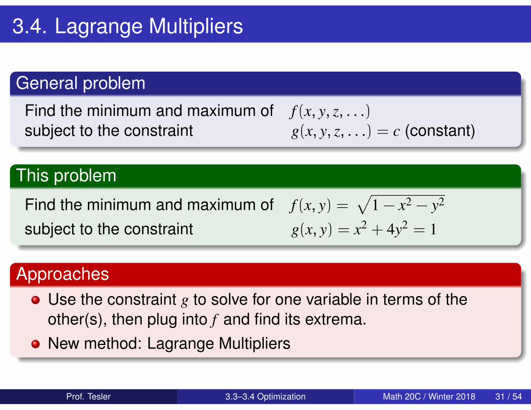
General problemFind the minimum and maximum of f (x, y, z, . . .)subject to the constraint g(x, y, z, . . .) = c (constant)
This problem
Find the minimum and maximum of f (x, y) =√
1 − x2 − y2
subject to the constraint g(x, y) = x2 + 4y2 = 1
ApproachesUse the constraint g to solve for one variable in terms of theother(s), then plug into f and find its extrema.New method: Lagrange Multipliers
Prof. Tesler 3.3–3.4 Optimization Math 20C / Winter 2018 31 / 54

Lagrange Multipliers
−1.0 −0.5 0.0 0.5 1.0
−1.0
−0.5
0.0
0.5
1.0
On the contour map, when the trail (g(x, y) = c, in red) crosses acontour of f (x, y), f is lower on one side and higher on the other.
The min/max of f (x, y) on the trail occurs when the trail is tangentto a contour of f (x, y)! The trail goes up to a max and then backdown, staying on the same side of the contour of f .
Recall ∇f ⊥ contours of f ∇g ⊥ contours of gSo contours of f and g are tangent when ∇f‖∇g, or ∇f = λ∇g forsome scalar λ (called a Lagrange Multiplier ).
Prof. Tesler 3.3–3.4 Optimization Math 20C / Winter 2018 32 / 54
Lagrange Multipliers for the ellipse path
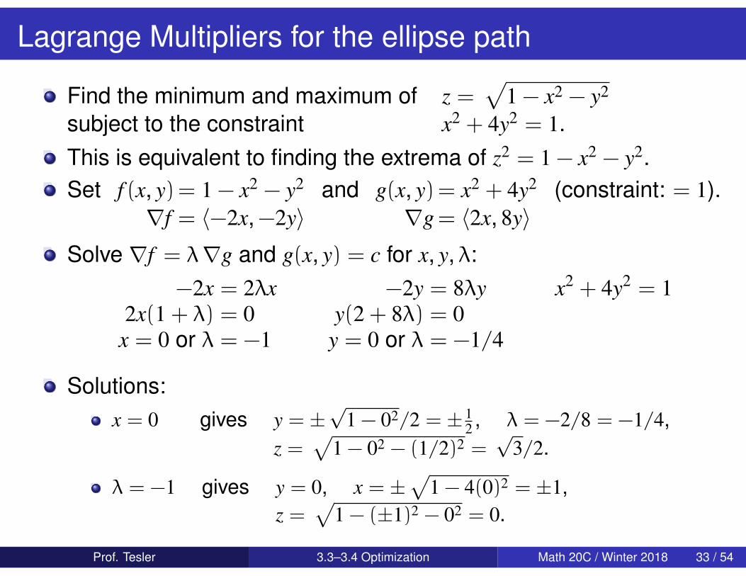
Find the minimum and maximum of z =√
1 − x2 − y2
subject to the constraint x2 + 4y2 = 1.This is equivalent to finding the extrema of z2 = 1 − x2 − y2.Set f (x, y)= 1 − x2 − y2
∇f = 〈−2x,−2y〉and g(x, y)= x2 + 4y2
∇g= 〈2x, 8y〉(constraint: = 1).
Solve ∇f = λ∇g and g(x, y) = c for x, y, λ:−2x = 2λx −2y = 8λy x2 + 4y2 = 1
2x(1 + λ) = 0 y(2 + 8λ) = 0x = 0 or λ = −1 y = 0 or λ = −1/4
Solutions:x = 0 gives y = ±
√1 − 02/2 = ± 1
2 , λ = −2/8 = −1/4,z =
√1 − 02 − (1/2)2 =
√3/2.
λ = −1 gives y = 0, x = ±√
1 − 4(0)2 = ±1,z =
√1 − (±1)2 − 02 = 0.
Prof. Tesler 3.3–3.4 Optimization Math 20C / Winter 2018 33 / 54
Lagrange Multipliers for the ellipse path
√1 − x2 − y2 is continuous along the closed path x2 + 4y2 = 1, so
z =√
32 at (x, y) = (0,± 1
2 ) are absolute maxima
z = 0 at (x, y) = (±1, 0) are absolute minima
λ is a tool to solve for the extremal points; its value isn’t important.
Prof. Tesler 3.3–3.4 Optimization Math 20C / Winter 2018 34 / 54
Lagrange Multipliers on Closed Region with Boundary
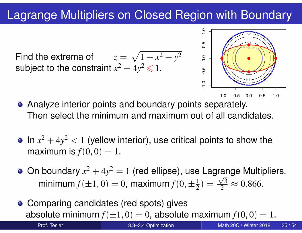
Find the extrema of z =√
1 − x2 − y2
subject to the constraint x2 + 4y2 6 1.
−1.0 −0.5 0.0 0.5 1.0
−1.0
−0.5
0.0
0.5
1.0
●
●
●
●●
Analyze interior points and boundary points separately.Then select the minimum and maximum out of all candidates.
In x2 + 4y2 < 1 (yellow interior), use critical points to show themaximum is f (0, 0) = 1.
On boundary x2 + 4y2 = 1 (red ellipse), use Lagrange Multipliers.minimum f (±1, 0) = 0, maximum f (0,± 1
2) =√
32 ≈ 0.866.
Comparing candidates (red spots) givesabsolute minimum f (±1, 0) = 0, absolute maximum f (0, 0) = 1.
Prof. Tesler 3.3–3.4 Optimization Math 20C / Winter 2018 35 / 54
Example: Rectangular boxMethod 1: Critical points
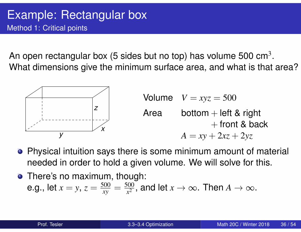
An open rectangular box (5 sides but no top) has volume 500 cm3.What dimensions give the minimum surface area, and what is that area?
y
z
x
Volume V = xyz = 500
Area bottom + left & right+ front & back
A = xy + 2xz + 2yz
Physical intuition says there is some minimum amount of materialneeded in order to hold a given volume. We will solve for this.There’s no maximum, though:e.g., let x = y, z = 500
xy = 500x2 , and let x→∞. Then A→∞.
Prof. Tesler 3.3–3.4 Optimization Math 20C / Winter 2018 36 / 54
Example: Rectangular boxMethod 1: Critical points
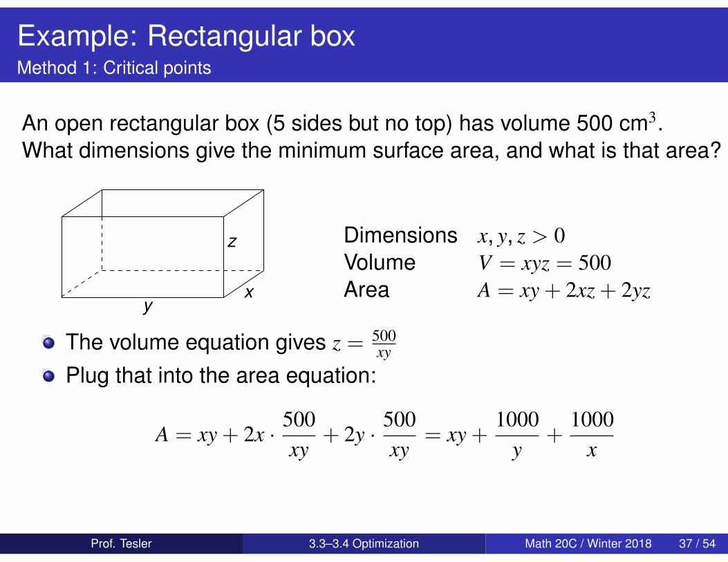
An open rectangular box (5 sides but no top) has volume 500 cm3.What dimensions give the minimum surface area, and what is that area?
y
z
x
Dimensions x, y, z > 0Volume V = xyz = 500Area A = xy + 2xz + 2yz
The volume equation gives z = 500xy
Plug that into the area equation:
A = xy + 2x · 500xy
+ 2y · 500xy
= xy +1000
y+
1000x
Prof. Tesler 3.3–3.4 Optimization Math 20C / Winter 2018 37 / 54
Example: Rectangular boxMethod 1: Critical points
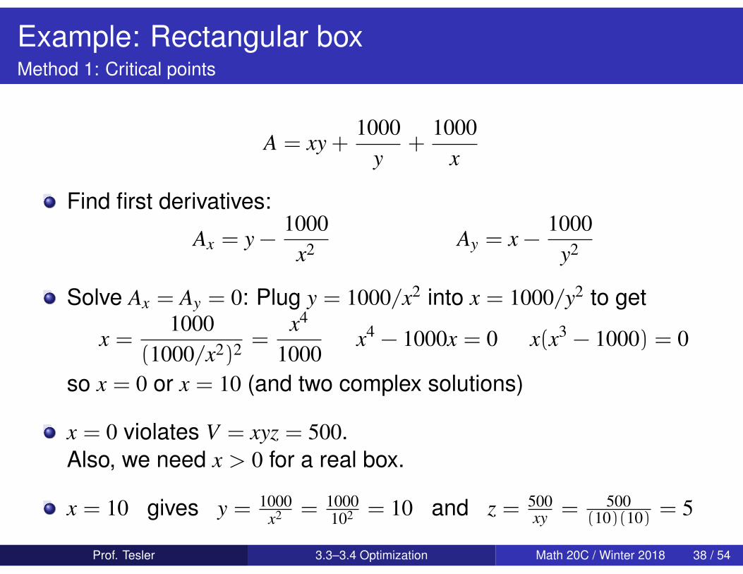
A = xy +1000
y+
1000x
Find first derivatives:
Ax = y −1000
x2 Ay = x −1000
y2
Solve Ax = Ay = 0: Plug y = 1000/x2 into x = 1000/y2 to get
x =1000
(1000/x2)2 =x4
1000x4 − 1000x = 0 x(x3 − 1000) = 0
so x = 0 or x = 10 (and two complex solutions)
x = 0 violates V = xyz = 500.Also, we need x > 0 for a real box.
x = 10 gives y = 1000x2 = 1000
102 = 10 and z = 500xy = 500
(10)(10) = 5
Prof. Tesler 3.3–3.4 Optimization Math 20C / Winter 2018 38 / 54
Example: Rectangular boxMethod 1: Critical points
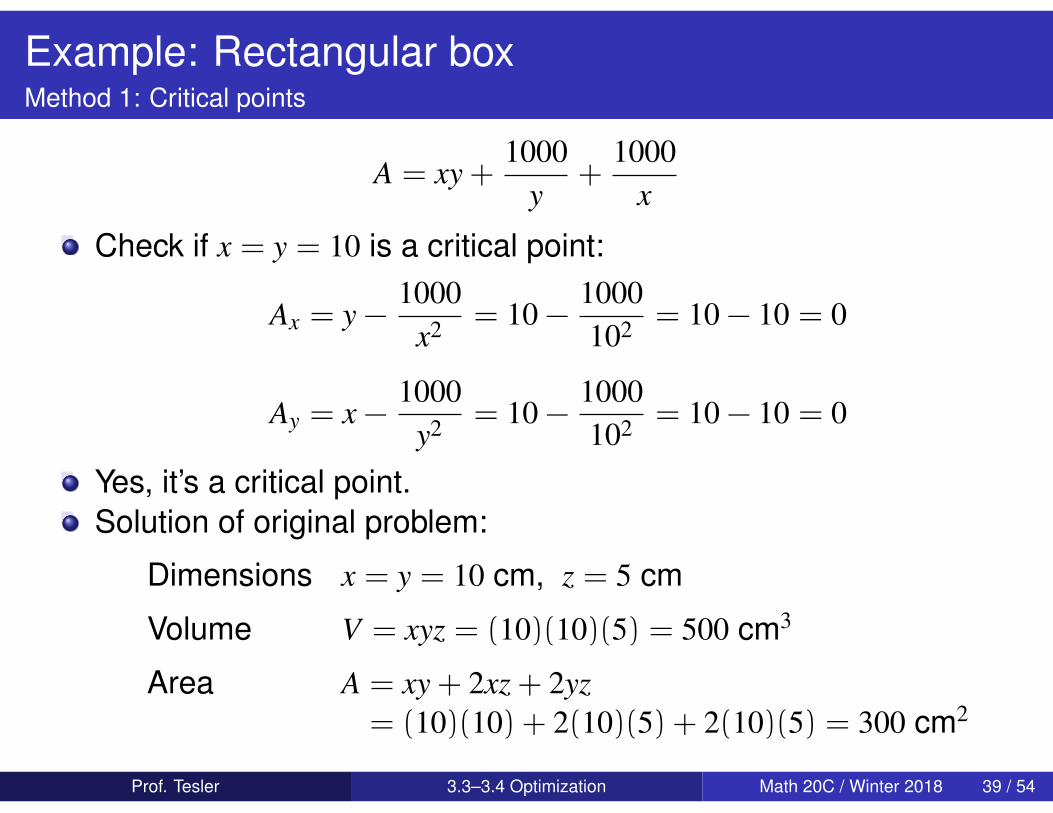
A = xy +1000
y+
1000x
Check if x = y = 10 is a critical point:
Ax = y −1000
x2 = 10 −1000102 = 10 − 10 = 0
Ay = x −1000
y2 = 10 −1000102 = 10 − 10 = 0
Yes, it’s a critical point.Solution of original problem:
Dimensions x = y = 10 cm, z = 5 cm
Volume V = xyz = (10)(10)(5) = 500 cm3
Area A = xy + 2xz + 2yz= (10)(10) + 2(10)(5) + 2(10)(5) = 300 cm2
Prof. Tesler 3.3–3.4 Optimization Math 20C / Winter 2018 39 / 54
Example: Rectangular boxMethod 1: Critical points
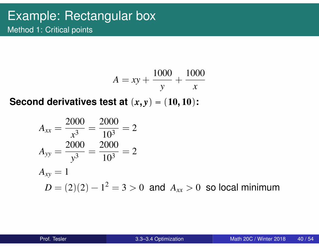
A = xy +1000
y+
1000x
Second derivatives test at (x, y) = (10, 10):
Axx =2000
x3 =2000103 = 2
Ayy =2000
y3 =2000103 = 2
Axy = 1
D = (2)(2) − 12 = 3 > 0 and Axx > 0 so local minimum
Prof. Tesler 3.3–3.4 Optimization Math 20C / Winter 2018 40 / 54
Example: Rectangular boxMethod 1: Critical points Using gradients instead of 2nd derivatives test
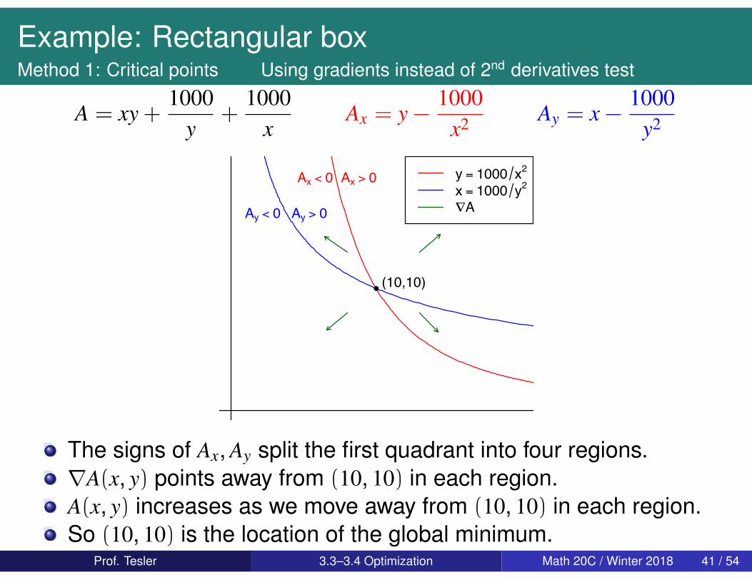
A = xy +1000
y+
1000x
Ax = y −1000
x2 Ay = x −1000
y2
!(10,10)
Ax < 0 Ax > 0
Ay > 0Ay < 0
y = 1000 x2x = 1000 y2!A
The signs of Ax, Ay split the first quadrant into four regions.∇A(x, y) points away from (10, 10) in each region.A(x, y) increases as we move away from (10, 10) in each region.So (10, 10) is the location of the global minimum.
Prof. Tesler 3.3–3.4 Optimization Math 20C / Winter 2018 41 / 54
Example: Rectangular boxMethod 2: Lagrange Multipliers
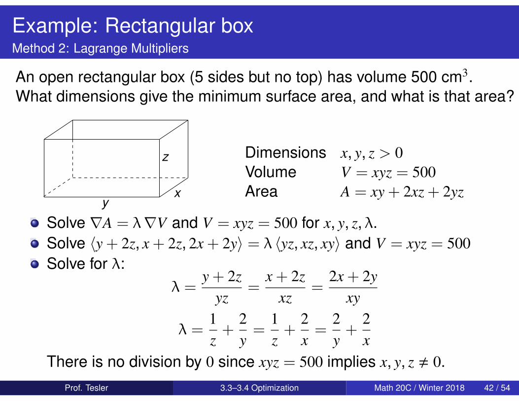
An open rectangular box (5 sides but no top) has volume 500 cm3.What dimensions give the minimum surface area, and what is that area?
y
z
x
Dimensions x, y, z > 0Volume V = xyz = 500Area A = xy + 2xz + 2yz
Solve ∇A = λ∇V and V = xyz = 500 for x, y, z, λ.Solve 〈y + 2z, x + 2z, 2x + 2y〉 = λ 〈yz, xz, xy〉 and V = xyz = 500Solve for λ:
λ =y + 2z
yz=
x + 2zxz
=2x + 2y
xy
λ =1z+
2y=
1z+
2x=
2y+
2x
There is no division by 0 since xyz = 500 implies x, y, z , 0.Prof. Tesler 3.3–3.4 Optimization Math 20C / Winter 2018 42 / 54
Example: Rectangular boxMethod 2: Lagrange Multipliers
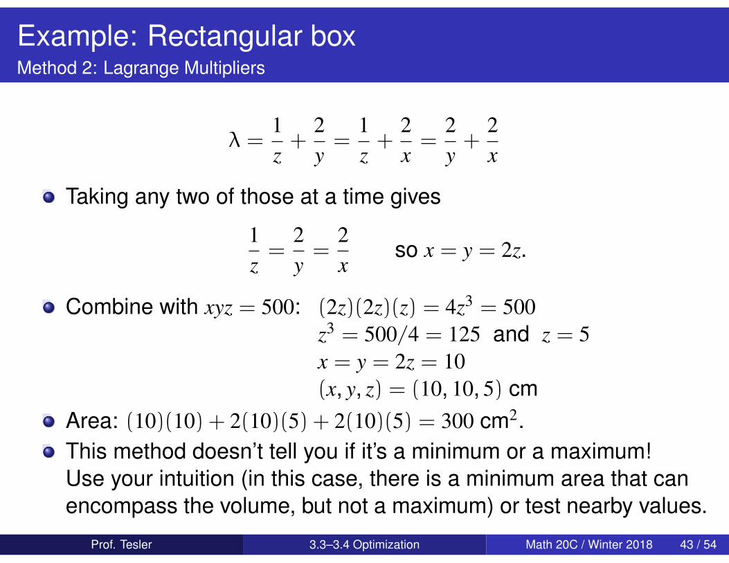
λ =1z+
2y=
1z+
2x=
2y+
2x
Taking any two of those at a time gives
1z=
2y=
2x
so x = y = 2z.
Combine with xyz = 500: (2z)(2z)(z) = 4z3 = 500z3 = 500/4 = 125 and z = 5x = y = 2z = 10(x, y, z) = (10, 10, 5) cm
Area: (10)(10) + 2(10)(5) + 2(10)(5) = 300 cm2.This method doesn’t tell you if it’s a minimum or a maximum!Use your intuition (in this case, there is a minimum area that canencompass the volume, but not a maximum) or test nearby values.
Prof. Tesler 3.3–3.4 Optimization Math 20C / Winter 2018 43 / 54
Example: Rectangular boxMethod 2: Lagrange Multipliers
This method doesn’t tell you if it’s a minimum or a maximum!Use your intuition (in this case, there is a minimum area that canencompass the volume, but not a maximum) or test nearby values.
Surface xyz = 500 (with x, y, z > 0) is not bounded, so ExtremeValue Theorem doesn’t apply. No guarantee there’s a globalmin/max in the region.
Only one candidate point, so we can’t compare candidates.
Pages 197–201 extend the 2nd derivatives test to constraintequations, but it uses Linear Algebra (Math 18).
Prof. Tesler 3.3–3.4 Optimization Math 20C / Winter 2018 44 / 54
Example: Function of 10 variables
Find 10 positive #’s whose sum is 1000 and whose product is maximized:
Maximize f (x1, . . . , x10) = x1 x2 . . . x10 ∇f =⟨
fx1
, . . . , fx10
⟩Subject to g(x1, . . . , x10) = x1 + · · ·+ x10 = 1000 ∇g = 〈1, . . . , 1〉
Solve ∇f = λ∇g: fx1
= · · · = fx10
= λ · 1x1 = · · · = x10
Combine with constraint g = x1 + · · ·+ x10 = 1000:10 x1 = 1000 so x1 = · · · = x10 = 100
The product is 10010 = 1020. This turns out to be the maximum.
Minimum: as any of the variables approach 0, the productapproaches 0, without reaching it. So, in the domainx1, . . . , x10 > 0, the minimum does not exist.
Prof. Tesler 3.3–3.4 Optimization Math 20C / Winter 2018 45 / 54
Closest point on a plane to the origin
x
z
y
O
P
Q
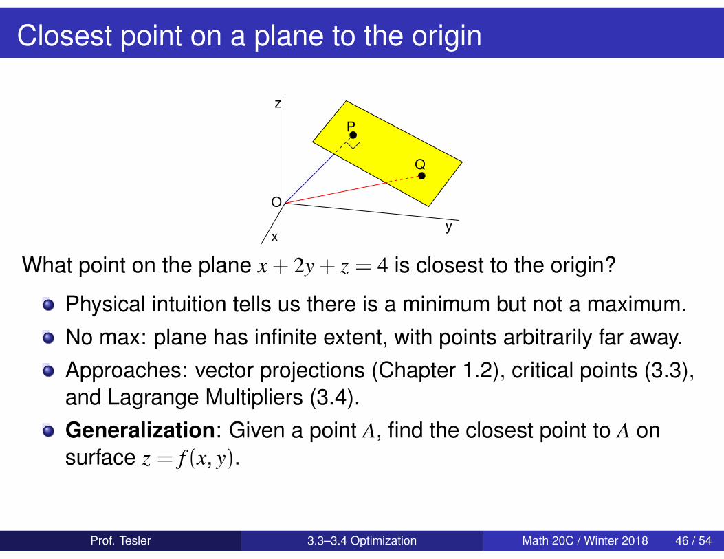
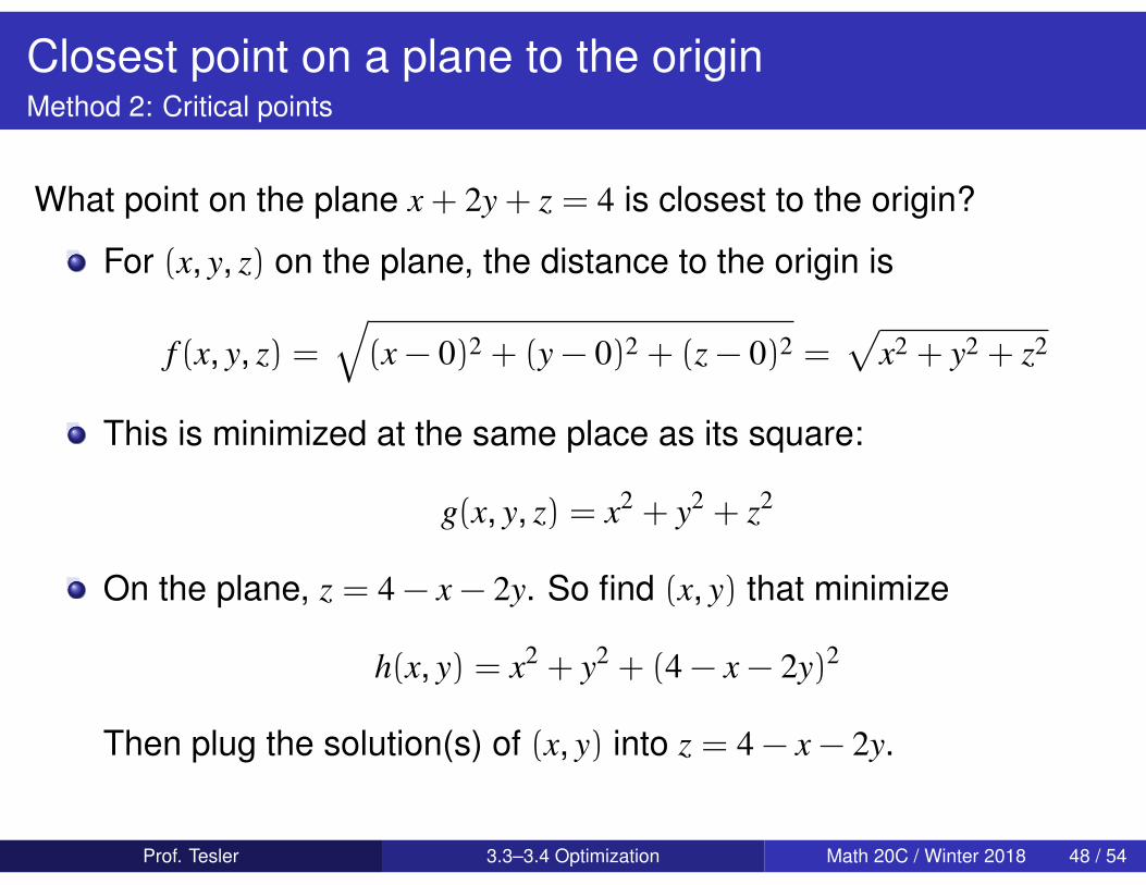
What point on the plane x + 2y + z = 4 is closest to the origin?
Physical intuition tells us there is a minimum but not a maximum.No max: plane has infinite extent, with points arbitrarily far away.Approaches: vector projections (Chapter 1.2), critical points (3.3),and Lagrange Multipliers (3.4).Generalization: Given a point A, find the closest point to A onsurface z = f (x, y).
Prof. Tesler 3.3–3.4 Optimization Math 20C / Winter 2018 46 / 54
Closest point on a plane to the originMethod 1: Projection
x
z
y
O
P
Q
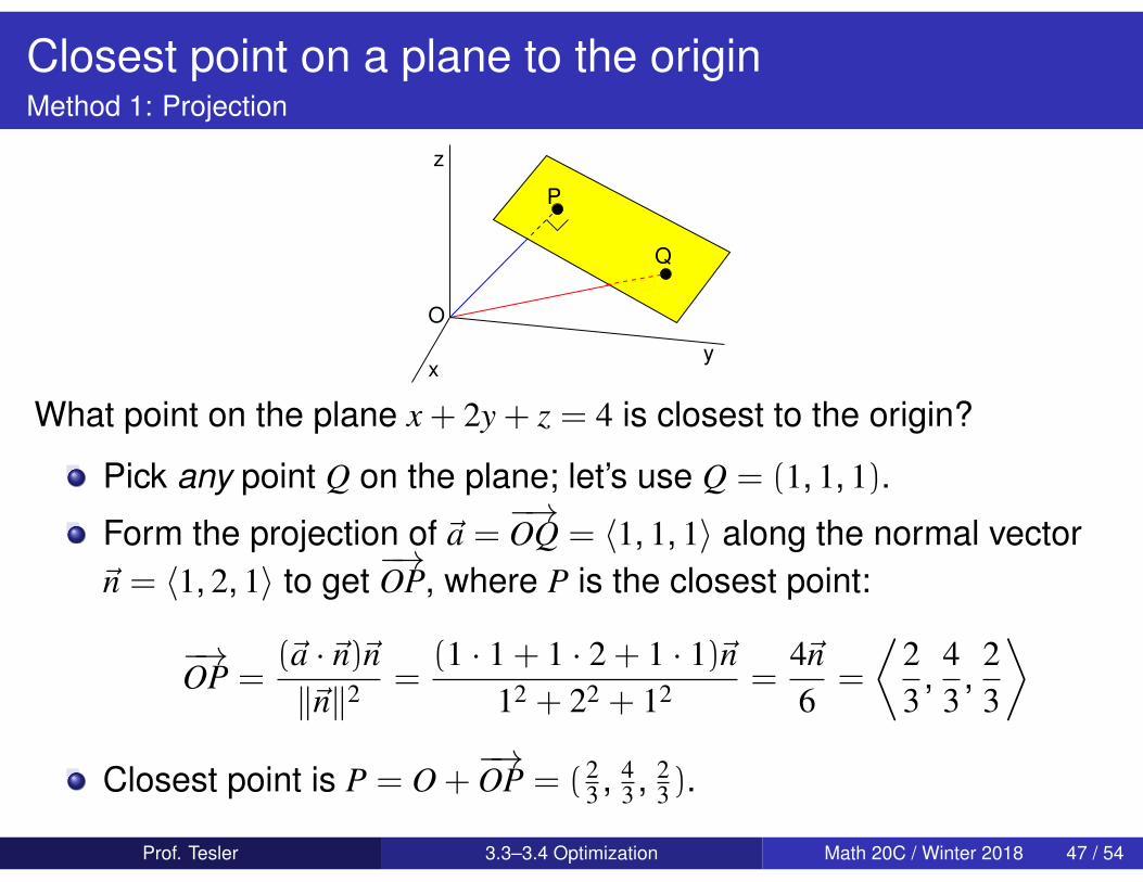
What point on the plane x + 2y + z = 4 is closest to the origin?
Pick any point Q on the plane; let’s use Q = (1, 1, 1).
Form the projection of ~a =−→OQ = 〈1, 1, 1〉 along the normal vector
~n = 〈1, 2, 1〉 to get−→OP, where P is the closest point:
−→OP =
(~a ·~n)~n‖~n‖2 =
(1 · 1 + 1 · 2 + 1 · 1)~n12 + 22 + 12 =
4~n6
=
⟨23
,43
,23
⟩Closest point is P = O +
−→OP = (2
3 , 43 , 2
3).
Prof. Tesler 3.3–3.4 Optimization Math 20C / Winter 2018 47 / 54
Closest point on a plane to the originMethod 2: Critical points
What point on the plane x + 2y + z = 4 is closest to the origin?
For (x, y, z) on the plane, the distance to the origin is
f (x, y, z) =√
(x − 0)2 + (y − 0)2 + (z − 0)2 =√
x2 + y2 + z2
This is minimized at the same place as its square:
g(x, y, z) = x2 + y2 + z2
On the plane, z = 4 − x − 2y. So find (x, y) that minimize
h(x, y) = x2 + y2 + (4 − x − 2y)2
Then plug the solution(s) of (x, y) into z = 4 − x − 2y.
Prof. Tesler 3.3–3.4 Optimization Math 20C / Winter 2018 48 / 54
Closest point on a plane to the originMethod 2: Critical points
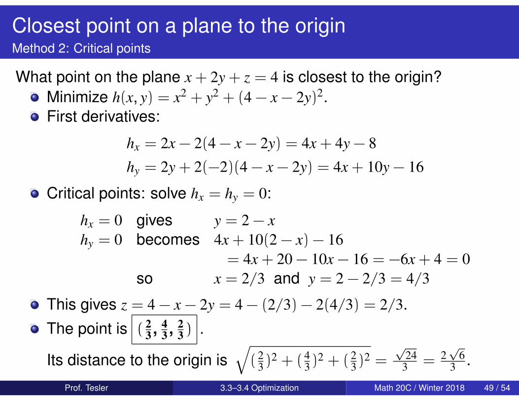
What point on the plane x + 2y + z = 4 is closest to the origin?Minimize h(x, y) = x2 + y2 + (4 − x − 2y)2.First derivatives:
hx = 2x − 2(4 − x − 2y) = 4x + 4y − 8
hy = 2y + 2(−2)(4 − x − 2y) = 4x + 10y − 16
Critical points: solve hx = hy = 0:
hx = 0 gives y = 2 − xhy = 0 becomes 4x + 10(2 − x) − 16
= 4x + 20 − 10x − 16 = −6x + 4 = 0so x = 2/3 and y = 2 − 2/3 = 4/3
This gives z = 4 − x − 2y = 4 − (2/3) − 2(4/3) = 2/3.
The point is ( 23 , 4
3 , 23) .
Its distance to the origin is√
( 23)
2 + ( 43)
2 + ( 23)
2 =√
243 = 2
√6
3 .
Prof. Tesler 3.3–3.4 Optimization Math 20C / Winter 2018 49 / 54
Closest point on a plane to the originMethod 2: Critical points
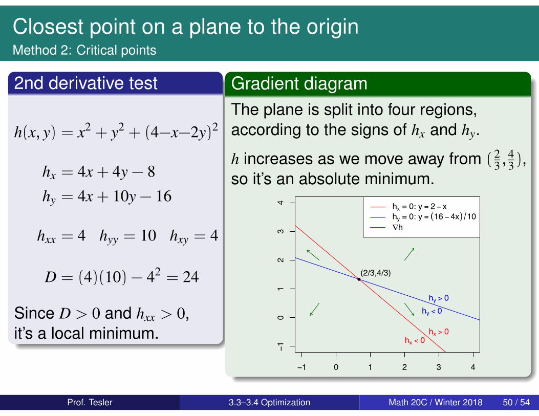
2nd derivative test
h(x, y) = x2 + y2 + (4−x−2y)2
hx = 4x + 4y − 8
hy = 4x + 10y − 16
hxx = 4 hyy = 10 hxy = 4
D = (4)(10) − 42 = 24
Since D > 0 and hxx > 0,it’s a local minimum.
Gradient diagramThe plane is split into four regions,according to the signs of hx and hy.
h increases as we move away from ( 23 , 4
3),so it’s an absolute minimum.
−1 0 1 2 3 4
−10
12
34
!
(2/3,4/3)
hx > 0hx < 0
hy > 0hy < 0
hx = 0: y = 2 ! xhy = 0: y = (16 ! 4x) 10"h
Prof. Tesler 3.3–3.4 Optimization Math 20C / Winter 2018 50 / 54

Closest point on a plane to the originMethod 3: Lagrange Multipliers
What point on the plane z = 4 − x − 2y is closest to the origin?
Rewrite this as a constraint function = constant: x + 2y + z = 4
Minimize f (x, y, z) = x2 + y2 + z2 (square of distance to origin)Subject to g(x, y, z) = x + 2y + z = 4 (constraint: on plane)
Solve ∇f = λ∇g and x + 2y + z = 4:〈2x, 2y, 2z〉 = λ 〈1, 2, 1〉 x + 2y + z = 4
2x = λ · 1 2y = λ · 2 2z = λ · 1
x = λ2 y = λ z = λ
2λ2 + 2λ+ λ
2 = 3λ = 4 so λ = 43
x = 23 y = 4
3 z = 23
The closest point is ( 23 , 4
3 , 23).
Its distance to the origin is√
( 23)
2 + ( 43)
2 + ( 23)
2 =√
249 = 2
√6
3 .
Prof. Tesler 3.3–3.4 Optimization Math 20C / Winter 2018 51 / 54
Closest point on a surface to a given point
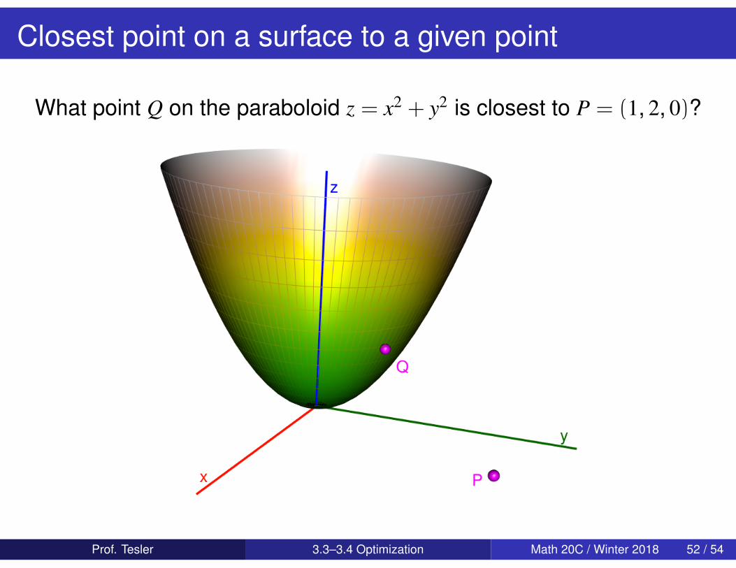
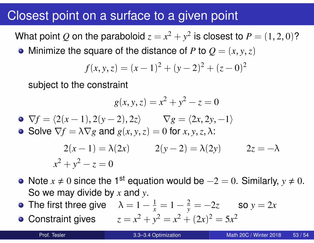
What point Q on the paraboloid z = x2 + y2 is closest to P = (1, 2, 0)?
Prof. Tesler 3.3–3.4 Optimization Math 20C / Winter 2018 52 / 54
Closest point on a surface to a given point
What point Q on the paraboloid z = x2 + y2 is closest to P = (1, 2, 0)?Minimize the square of the distance of P to Q = (x, y, z)
f (x, y, z) = (x − 1)2 + (y − 2)2 + (z − 0)2
subject to the constraint
g(x, y, z) = x2 + y2 − z = 0
∇f = 〈2(x − 1), 2(y − 2), 2z〉 ∇g = 〈2x, 2y,−1〉Solve ∇f = λ∇g and g(x, y, z) = 0 for x, y, z, λ:
2(x − 1) = λ(2x) 2(y − 2) = λ(2y) 2z = −λ
x2 + y2 − z = 0
Note x , 0 since the 1st equation would be −2 = 0. Similarly, y , 0.So we may divide by x and y.The first three give λ = 1 − 1
x = 1 − 2y = −2z so y = 2x
Constraint gives z = x2 + y2 = x2 + (2x)2 = 5x2
Prof. Tesler 3.3–3.4 Optimization Math 20C / Winter 2018 53 / 54
Closest point on a surface to a given point
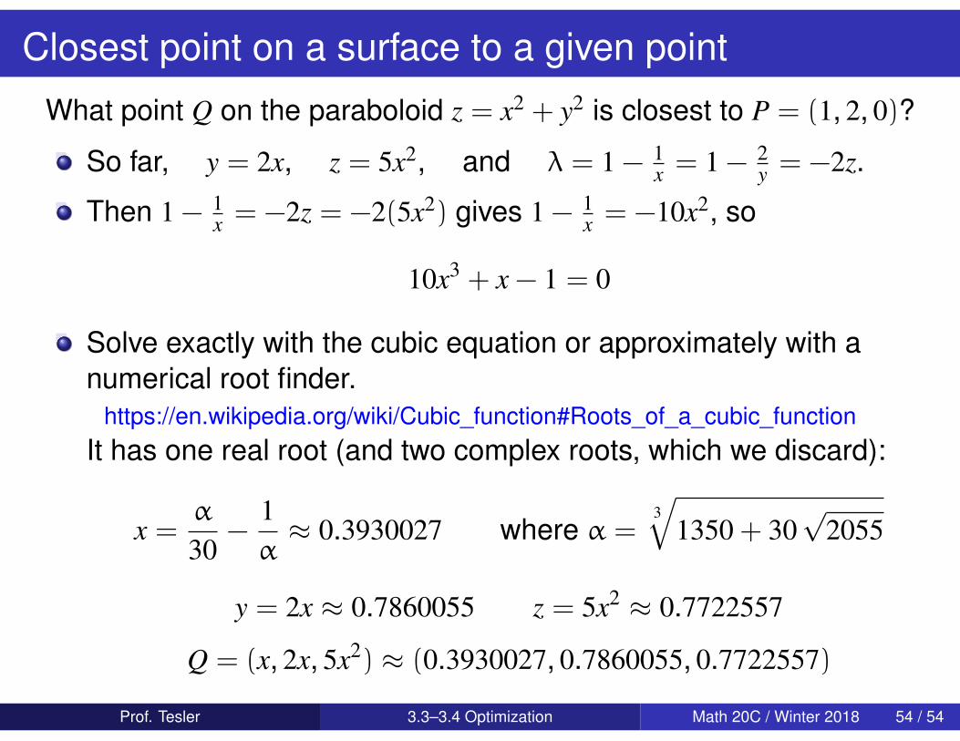
What point Q on the paraboloid z = x2 + y2 is closest to P = (1, 2, 0)?
So far, y = 2x, z = 5x2, and λ = 1 − 1x = 1 − 2
y = −2z.
Then 1 − 1x = −2z = −2(5x2) gives 1 − 1
x = −10x2, so
10x3 + x − 1 = 0
Solve exactly with the cubic equation or approximately with anumerical root finder.
https://en.wikipedia.org/wiki/Cubic_function#Roots_of_a_cubic_functionIt has one real root (and two complex roots, which we discard):
x =α
30−
1α≈ 0.3930027 where α =
3√
1350 + 30√
2055
y = 2x ≈ 0.7860055 z = 5x2 ≈ 0.7722557
Q = (x, 2x, 5x2) ≈ (0.3930027, 0.7860055, 0.7722557)
Prof. Tesler 3.3–3.4 Optimization Math 20C / Winter 2018 54 / 54