Embed Size (px)
Citation preview
WJ-25 DESIGN PRPOSAL
Proposal for the next generation of Single-Engine Turboprop aircraft
In Response to AIAA 2016-2017 Undergraduate Team Design Competition Request for Proposal
Team Leader: Zhang Yingao Team Member: Wen Mengyang & Wang Haonan
Faculty Advisor: Dr. Chih-Jen Sung

SIGNATURE PAGE
Design Team:
Zhang Yingao:
#762521
Wen Mengyang:
#774336
Wang Haonan:
#774661

Acknowledgements
The authors would like to thank the following individuals who were instrumental
in the success of this engine design:
Dr. Chih-Jen Sung for his tremendous help in completing this proposal.
Dr. Xin Hui for his comprehensive support and supervision
Dr. Xi Wang for his advice on off-design and transient performance
Our colleague Wang Xinyao for his assistance on combustion system design
Our senior Yang Shubo for his instructions on MATLAB
All the teachers, students and facilities who have aided.
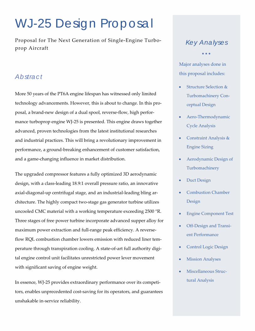
WJ-25 Design Proposal Proposal for The Next Generation of Single-Engine Turbo-prop Aircraft
Abstract
More 50 years of the PT6A engine lifespan has witnessed only limited
technology advancements. However, this is about to change. In this pro-
posal, a brand-new design of a dual spool, reverse-flow, high perfor-
mance turboprop engine WJ-25 is presented. This engine draws together
advanced, proven technologies from the latest institutional researches
and industrial practices. This will bring a revolutionary improvement in
performance, a ground-breaking enhancement of customer satisfaction,
and a game-changing influence in market distribution.
The upgraded compressor features a fully optimized 3D aerodynamic
design, with a class-leading 18.9:1 overall pressure ratio, an innovative
axial-diagonal-up centrifugal stage, and an industrial-leading bling ar-
chitecture. The highly compact two-stage gas generator turbine utilizes
uncooled CMC material with a working temperature exceeding 2500 °R.
Three stages of free power turbine incorporate advanced supper alloy for
maximum power extraction and full-range peak efficiency. A reverse-
flow RQL combustion chamber lowers emission with reduced liner tem-
perature through transpiration cooling. A state-of-art full authority digi-
tal engine control unit facilitates unrestricted power lever movement
with significant saving of engine weight.
In essence, WJ-25 provides extraordinary performance over its competi-
tors, enables unprecedented cost-saving for its operators, and guarantees
unshakable in-service reliability.
Key Analyses • • •
Major analyses done in
this proposal includes:
• Structure Selection &
Turbomachinery Con-
ceptual Design
• Aero-Thermodynamic
Cycle Analysis
• Constraint Analysis &
Engine Sizing
• Aerodynamic Design of
Turbomachinery
• Duct Design
• Combustion Chamber
Design
• Engine Component Test
• Off-Design and Transi-
ent Performance
• Control Logic Design
• Mission Analyses
• Miscellaneous Struc-
tural Analysis
Performance
Maximum speed 370KEAS
Cruise speed 337KTAS
Mission Fuel Burn 1410.233501 lb.
Cruise BSFC 0.415085047
Takeoff BSFC 0.443762418
Engine Weight No more than 543.4lb
Engine Diameter 19 Inch
Required Trade Studies
Engine Cycle Design Space Carpet Plots Page # 20
In-Depth Cycle Summary Page # 31
Final engine flow path (Page #) 89
Final cycle study using chosen cycle program (Page #) 79
Detailed stage-by-stage turbomachinery design information (page # for each
component)
HPT: 33, LPT: 40,
AC: 50, CC: 54
Detailed design of velocity triangles for first stage of each component (list
page #’s and component)
HPT: 39, LPT: 47
AC: 53, CC: 58
Table RFP-1 Compliance Matrix
Summary Data
Design MN 0
Design Altitude 0
Design Shaft Horsepower 2087.642072
Design BSFC 0.449675766
Design Overall Pressure Ratio 18.9
Design T4.1 2654.986132
Design Engine Pressure Ratio 18.9
Design Chargeable Cooling Flow (%@25) 0
Design Non-Chargeable Cooling Flow (%@25) 0
Design Adiabatic Efficiency for Each Turbine 0.907495807@HPT
0.808984908@FPT
Design Polytropic Efficiency for Each Compressor AC: 0.8676, CC: 0.8990
Design Shaft Power Loss 0.5%
Design HP/IP/LP/PT Shaft RPM 41093.59326@HP
21041. 2598@LP 1
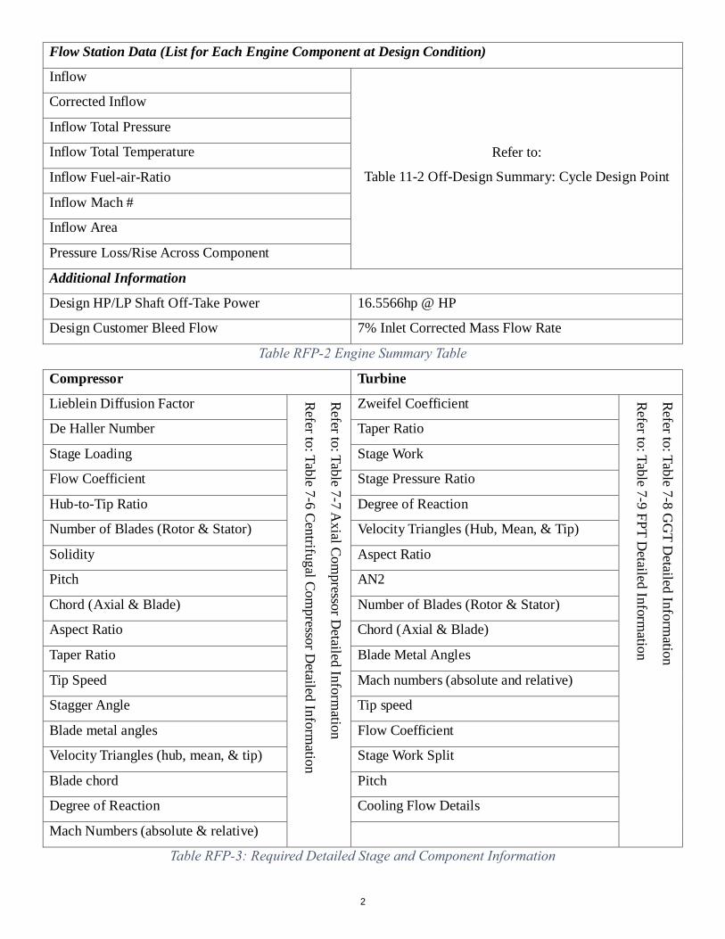
Flow Station Data (List for Each Engine Component at Design Condition)
Inflow
Refer to:
Table 11-2 Off-Design Summary: Cycle Design Point
Corrected Inflow
Inflow Total Pressure
Inflow Total Temperature
Inflow Fuel-air-Ratio
Inflow Mach #
Inflow Area
Pressure Loss/Rise Across Component
Additional Information
Design HP/LP Shaft Off-Take Power 16.5566hp @ HP
Design Customer Bleed Flow 7% Inlet Corrected Mass Flow Rate
Table RFP-2 Engine Summary Table
Compressor Turbine
Lieblein Diffusion Factor Refer to: Table 7-7 Axial Com
pressor Detailed Inform
ation
Refer to: Table 7-6 Centrifugal Compressor D
etailed Information
Zweifel Coefficient Refer to: Table 7-8 GG
T Detailed Inform
ation
Refer to: Table 7-9 FPT Detailed Inform
ation
De Haller Number Taper Ratio
Stage Loading Stage Work
Flow Coefficient Stage Pressure Ratio
Hub-to-Tip Ratio Degree of Reaction
Number of Blades (Rotor & Stator) Velocity Triangles (Hub, Mean, & Tip)
Solidity Aspect Ratio
Pitch AN2
Chord (Axial & Blade) Number of Blades (Rotor & Stator)
Aspect Ratio Chord (Axial & Blade)
Taper Ratio Blade Metal Angles
Tip Speed Mach numbers (absolute and relative)
Stagger Angle Tip speed
Blade metal angles Flow Coefficient
Velocity Triangles (hub, mean, & tip) Stage Work Split
Blade chord Pitch
Degree of Reaction Cooling Flow Details
Mach Numbers (absolute & relative)
Table RFP-3: Required Detailed Stage and Component Information
2
Table of Contents
1. Introduction ............................................................................................................................................................................... 8
1.1. Architecture of This Proposal ......................................................................................................................................... 8
1.2. Customer Requirements, Market Research & Potential Technology Advancements ............................................... 9
2. Nomenclature & Station Numbering ..................................................................................................................................... 10
2.1. Station Numbers ............................................................................................................................................................ 10
2.2. Nomenclature ................................................................................................................................................................ 11
3. Structure Selection & Turbomachinery Conceptual Design ................................................................................................ 11
4. Aero-Thermodynamic Cycle Analysis ................................................................................................................................... 13
4.1. Design Point Selection .................................................................................................................................................. 13
4.2. Input Setup ..................................................................................................................................................................... 13
4.2.1. Ambient Condition................................................................................................................................................. 13
4.2.2. Axial-Centrifugal Compressor .............................................................................................................................. 14
4.2.3. Combustion Chamber ........................................................................................................................................... 14
4.2.4. Turbines ................................................................................................................................................................. 15
4.2.5. Ducts ...................................................................................................................................................................... 16
4.2.6. Engine Fuel ........................................................................................................................................................... 18
4.2.7. Secondary Air System .......................................................................................................................................... 18
4.2.8. Mechanical Losses ............................................................................................................................................... 18
4.2.9. Station Mach Number ........................................................................................................................................... 18
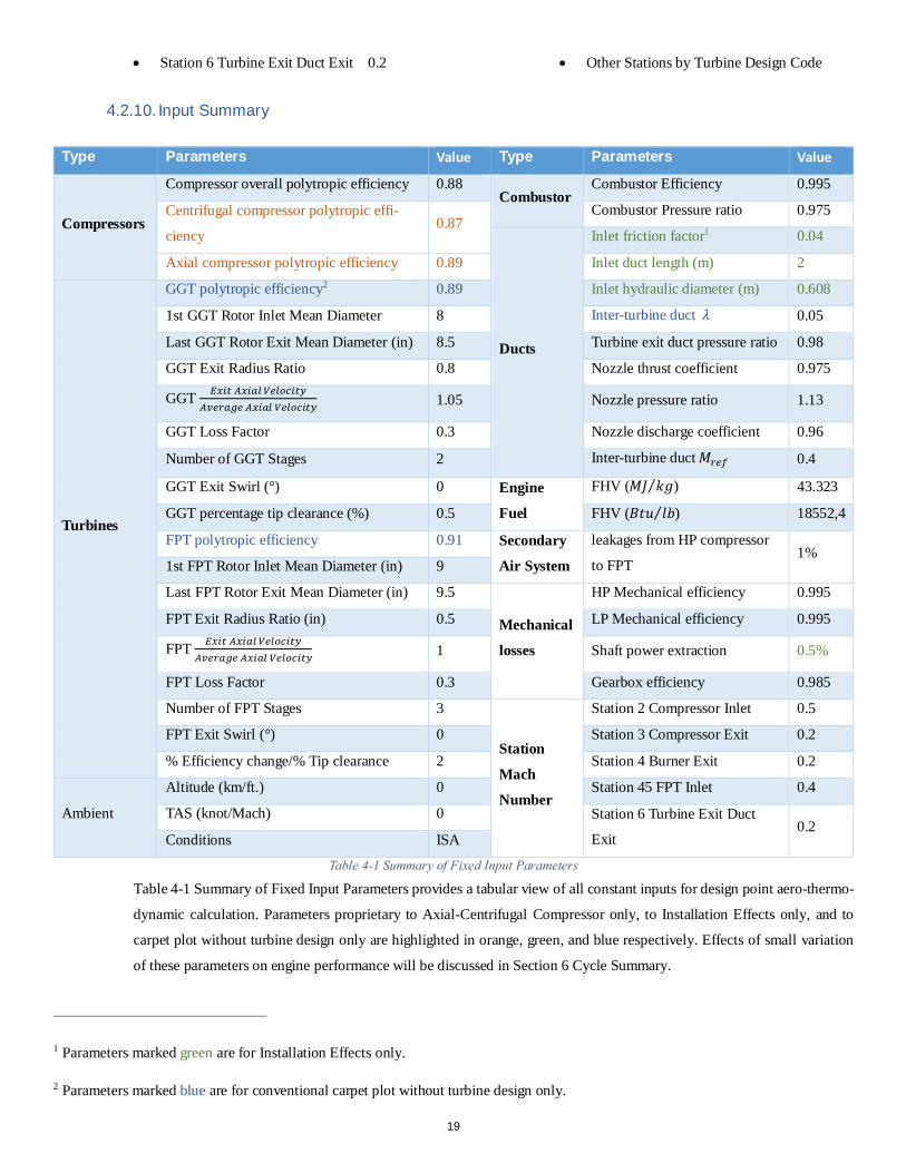
4.2.10. Input Summary ...................................................................................................................................................... 19
4.3. Carpet Plotting, Diagramming & Cycle Optimization .................................................................................................. 20
4.4. Summary of PR and COT Selections .......................................................................................................................... 25
3
5. Constraint Analysis & Engine Sizing ..................................................................................................................................... 25
5.1. Drag Polar Estimation ................................................................................................................................................... 25
5.2. Takeoff Constraints ....................................................................................................................................................... 26
5.3. Cruise Constraints ......................................................................................................................................................... 27
5.4. Maximum Speed Constraints ....................................................................................................................................... 27
5.5. Climb Rate & Service Ceiling Constraints ................................................................................................................... 27
5.6. Constraint Analysis Conclusion .................................................................................................................................... 28
5.7. Engine Sizing ................................................................................................................................................................. 29
6. Cycle Summary ...................................................................................................................................................................... 31
7. Aerodynamic Design of Turbomachinery ............................................................................................................................. 33
7.1. Gas Generator Turbine Design .................................................................................................................................... 33
7.1.1. GGT Preliminary Design ...................................................................................................................................... 33
7.1.2. GGT Design Space ............................................................................................................................................... 35
7.1.3. Manual Adjustment of Meridional Flow Path ...................................................................................................... 36
7.1.4. GGT S1 Optimization............................................................................................................................................ 36
7.1.5. GGT Blade Twist Factors ..................................................................................................................................... 37
7.1.6. GGT Streamline Analysis ..................................................................................................................................... 37
7.1.7. GGT Blade Profiling & 3D Design ....................................................................................................................... 39
7.2. Free Power Turbine Design.......................................................................................................................................... 40
7.2.1. FPT Preliminary Design........................................................................................................................................ 40
7.2.2. FPT Design Space ................................................................................................................................................ 43
7.2.3. Manual Adjustment of Meridional Flow Path ...................................................................................................... 43
7.2.4. FPT S1 Optimization............................................................................................................................................. 43
4
7.2.5. FPT Blade Twist Factors ...................................................................................................................................... 44
7.2.6. FPT Streamline Analysis ...................................................................................................................................... 45
7.2.7. FPT Blade Profiling & 3D Design ........................................................................................................................ 49
7.3. Pressure Ratio Separation Between Axial and Centrifugal Compressors ................................................................ 49
7.4. Axial Compressor Design ............................................................................................................................................. 50
7.4.1. Axial Compressor Preliminary Design................................................................................................................. 50
7.4.2. Axial Compressor Design Space ......................................................................................................................... 52
7.4.3. Axial Compressor Streamline Analysis ............................................................................................................... 53
7.4.4. Axial Compressor Profiling & 3D Design ............................................................................................................ 54
7.5. Centrifugal Compressor Design ................................................................................................................................... 54
7.5.1. Centrifugal Compressor Architecture .................................................................................................................. 54
7.5.2. Centrifugal Compressor Preliminary Design ...................................................................................................... 55
7.5.3. Centrifugal Compressor Design Space ............................................................................................................... 55
7.5.4. Centrifugal Compressor Streamline Analysis ..................................................................................................... 56
7.5.5. Centrifugal Compressor Profiling & 3D Design .................................................................................................. 58
7.6. Hand Calculation of Velocity Triangle .......................................................................................................................... 59
7.7. Detailed Component Information ................................................................................................................................. 60
8. Duct Design............................................................................................................................................................................. 64
8.1. Intake Design ................................................................................................................................................................. 64
8.1.1. Intake Sizing .......................................................................................................................................................... 64
8.1.2. Inlet Pressure Loss Estimation ............................................................................................................................ 66
8.1.3. Anti-Icing System .................................................................................................................................................. 67
8.2. Inter-Compressor and Inter-Turbine Duct ................................................................................................................... 68
5
9. Combustion Chamber Design ............................................................................................................................................... 68
9.1. Design Point Selection .................................................................................................................................................. 69
9.2. Pre-Diffuser Design ....................................................................................................................................................... 69
9.3. RQL Combustor Configuration ..................................................................................................................................... 70
9.4. Air Flow Distribution ...................................................................................................................................................... 71
9.4.1. Fuel Atomizing Flow ............................................................................................................................................. 71
9.4.2. Swirler Flow ........................................................................................................................................................... 71
9.4.3. Dome Cooling Flow .............................................................................................................................................. 72
9.4.4. Passage Air Flow, Dilution Flow and Liner Cooling Flow .................................................................................. 72
9.5. Combustion Chamber Sizing ........................................................................................................................................ 72
9.5.1. Reference Area Calculation ................................................................................................................................. 72
9.5.2. Dome and Passage Height .................................................................................................................................. 73
9.5.3. Number of Fuel Injectors and Length of Combustor .......................................................................................... 73
9.5.4. 3D Geometry of Combustion Chamber ............................................................................................................... 73
10. Engine Component Test ................................................................................................................................................... 73
10.1. Compressor Test ........................................................................................................................................................... 73
10.2. Turbine Test ................................................................................................................................................................... 74
10.3. Intake Map .................................................................................................................................................................... 75
10.4. Burner Lean Flame Out Limit ....................................................................................................................................... 75
11. Off-Design and Transient Performance ........................................................................................................................... 76
11.1. Steady-State Model Building and Verifications ........................................................................................................... 76
11.1.1. Steady-State Model Overview ............................................................................................................................. 76
11.1.2. Main Corrections and Modifications .................................................................................................................... 76
6
11.1.3. Steady-State Model Verification .......................................................................................................................... 78
11.1.4. Critical Off-Design Points ..................................................................................................................................... 78
11.2. Controller Design ........................................................................................................................................................... 81
11.2.1. Steady State Controller Design ........................................................................................................................... 81
11.2.2. Transient Controller Design ................................................................................................................................. 82
11.2.3. Control System Integration................................................................................................................................... 83
11.3. Transient Performance on Map .................................................................................................................................... 83
11.4. Mission Analyses ........................................................................................................................................................... 85
11.4.1. Mission Profile ....................................................................................................................................................... 85
11.4.2. Mission Analysis.................................................................................................................................................... 86
12. Miscellaneous Structural Issues ....................................................................................................................................... 88
12.1. Bearing Supports ........................................................................................................................................................... 88
12.2. Main Shaft Reduction Gearbox .................................................................................................................................... 89
12.3. Implementation of the Control Logic ............................................................................................................................ 89
13. 2D Engine Meridional Section View ................................................................................................................................. 89
14. References ......................................................................................................................................................................... 91
7
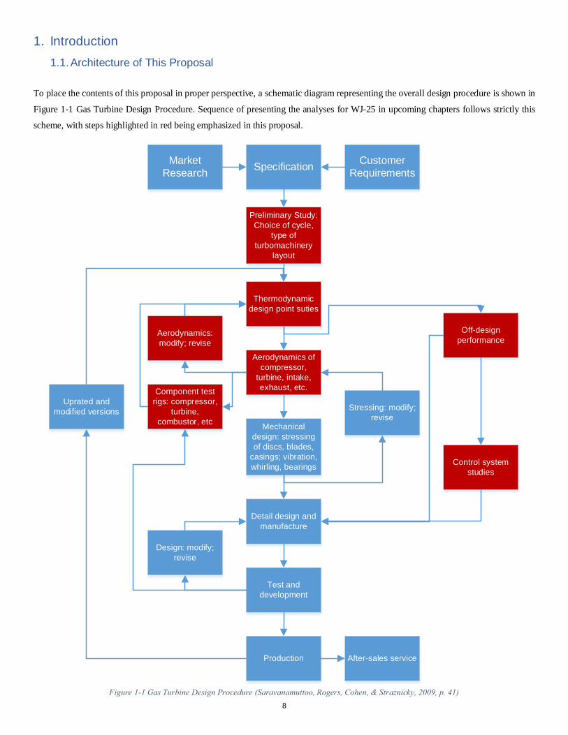
1. Introduction1.1. Architecture of This Proposal
To place the contents of this proposal in proper perspective, a schematic diagram representing the overall design procedure is shown in
Figure 1-1 Gas Turbine Design Procedure. Sequence of presenting the analyses for WJ-25 in upcoming chapters follows strictly this
scheme, with steps highlighted in red being emphasized in this proposal.
SpecificationMarket Research
Customer Requirements
Preliminary Study: Choice of cycle,
type of turbomachinery
layout
Thermodynamic design point suties
Aerodynamics of compressor,
turbine, intake, exhaust, etc.
Mechanical design: stressing of discs, blades,
casings; vibration, whirling, bearings
Off-design performance
Control system studies
Detail design and manufacture
Test and development
Production After-sales service
Stressing: modify; revise
Aerodynamics: modify; revise
Component test rigs: compressor,
turbine, combustor, etc
Design: modify; revise
Uprated and modified versions
Figure 1-1 Gas Turbine Design Procedure (Saravanamuttoo, Rogers, Cohen, & Straznicky, 2009, p. 41) 8
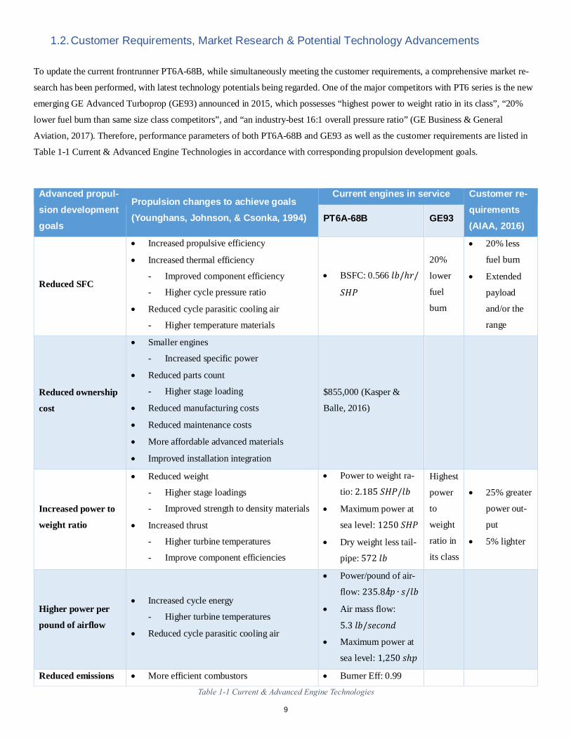
1.2. Customer Requirements, Market Research & Potential Technology Advancements
To update the current frontrunner PT6A-68B, while simultaneously meeting the customer requirements, a comprehensive market re-
search has been performed, with latest technology potentials being regarded. One of the major competitors with PT6 series is the new
emerging GE Advanced Turboprop (GE93) announced in 2015, which possesses “highest power to weight ratio in its class”, “20%
lower fuel burn than same size class competitors”, and “an industry-best 16:1 overall pressure ratio” (GE Business & General
Aviation, 2017). Therefore, performance parameters of both PT6A-68B and GE93 as well as the customer requirements are listed in
Table 1-1 Current & Advanced Engine Technologies in accordance with corresponding propulsion development goals.
Advanced propul-sion development goals
Propulsion changes to achieve goals (Younghans, Johnson, & Csonka, 1994)
Current engines in service Customer re-quirements (AIAA, 2016)
PT6A-68B GE93
Reduced SFC
• Increased propulsive efficiency
• Increased thermal efficiency
- Improved component efficiency
- Higher cycle pressure ratio
• Reduced cycle parasitic cooling air
- Higher temperature materials
• BSFC: 0.566 𝑙𝑙𝑙𝑙/ℎ𝑟𝑟/
𝑆𝑆𝑆𝑆𝑃𝑃
20%
lower
fuel
burn
• 20% less
fuel burn
• Extended
payload
and/or the
range
Reduced ownership
cost
• Smaller engines
- Increased specific power
• Reduced parts count
- Higher stage loading
• Reduced manufacturing costs
• Reduced maintenance costs
• More affordable advanced materials
• Improved installation integration
$855,000 (Kasper &
Balle, 2016)
Increased power to
weight ratio
• Reduced weight
- Higher stage loadings
- Improved strength to density materials
• Increased thrust
- Higher turbine temperatures
- Improve component efficiencies
• Power to weight ra-
tio: 2.185 𝑆𝑆𝑆𝑆𝑃𝑃/𝑙𝑙𝑙𝑙
• Maximum power at
sea level: 1250 𝑆𝑆𝑆𝑆𝑃𝑃
• Dry weight less tail-
pipe: 572 𝑙𝑙𝑙𝑙
Highest
power
to
weight
ratio in
its class
• 25% greater
power out-
put
• 5% lighter
Higher power per
pound of airflow
• Increased cycle energy
- Higher turbine temperatures
• Reduced cycle parasitic cooling air
• Power/pound of air-
flow: 235.8ℎ𝑝𝑝 ∙ 𝑠𝑠/𝑙𝑙𝑙𝑙
• Air mass flow:
5.3 𝑙𝑙𝑙𝑙/𝑠𝑠𝑠𝑠𝑠𝑠𝑠𝑠𝑠𝑠𝑠𝑠
• Maximum power at
sea level: 1,250 𝑠𝑠ℎ𝑝𝑝
Reduced emissions • More efficient combustors • Burner Eff: 0.99
Table 1-1 Current & Advanced Engine Technologies
9
After a quick scantling of technology emergence during re-
cent years, following features are incorporated into WJ-25:
• Ceramic-Matrix Composite in engine hot section
components. (Gardiner, 2015)
o Improved high-temp capability
o Reduced material density
• Carbon fiber reinforced polymer in engine casing
(Gardiner, 2015)
o Less component weight
o Increased material strength
o Better damping characteristics
• Axial-Diagonal-Up Centrifugal Compressor
• Bling and blisk stages
• RQL Combustor
• Transpiration combustor liner cooling
• Full authority digital engine control (FADEC)
The corresponding benefits of utilizing the above listed technologies are conspicuous when referring to Table 1-1 Current & Ad-
vanced Engine Technologies.
2. Nomenclature & Station Numbering
This section provides the standard of engine station numbering and nomenclature used for WJ-25. The general naming rule is adapted
from ARP 755A (SAE, 1974) with occasional reference towards AS681 Rev. E (SAE, 1989), ARP 1211A (SAE, 1974), ARP 1210A
(SAE, 1996), and ARP 1257 (SAE, 1989). Briefly, the basis of station numbering and engine nomenclature is described below, which
enables the reader to comprehend analyses throughout this proposal without referring to the standards listed above.
2.1. Station Numbers
1 Engine intake front flange, or leading edge
2 Axial compressor front face
24 Axial compressor exit face
25 Centrifugal compressor front face
3 Centrifugal compressor exit face
31 Compressor outlet diffuser exit/combustor inlet
4 Combustor exit plane
44 Gas generator turbine exit
45 Free power turbine nozzle guide vane leading edge
5 Free power turbine exit face
6 Turbine exit duct outlet face
8 Propelling nozzle throat
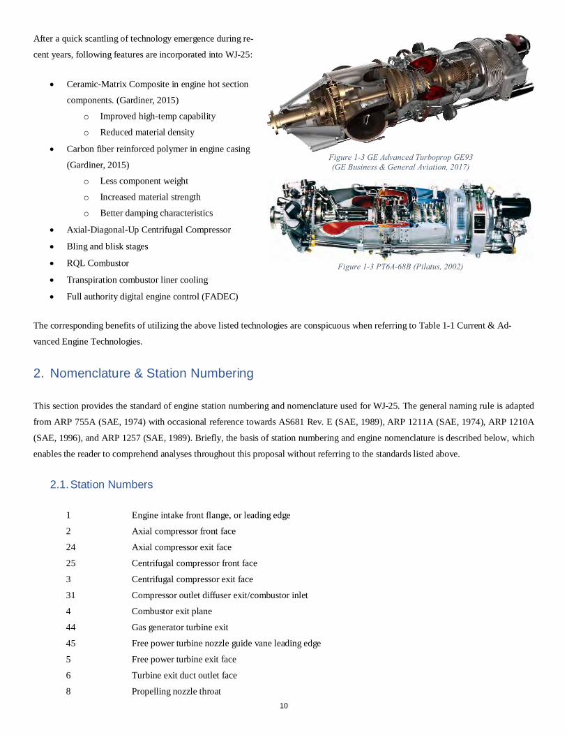
Figure 1-3 GE Advanced Turboprop GE93 (GE Business & General Aviation, 2017)
Figure 1-3 PT6A-68B (Pilatus, 2002)
10
2.2. Nomenclature
The symbols for mass flow, pressures and other quantities are defined as follows:
A Area
alt Altitude
amb Ambient
ax Axial
Bld Bleed
corr Corrected
C Constant value, coefficient
CFG Thrust coefficient
Cl Cooling
CMC Ceramic matrix composite
COT Combustor outlet temperature
d Diameter
dH Enthalpy difference
dp Design point
f Fuel
F Thrust
FAR Fuel-air-ratio
FPT Free power turbine
FHV Lower Heating Value of Fuel
GGT Gas Generator Turbine
H Enthalpy
HP High-pressure
HPT High pressure turbine
ISA International standard atmos-
phere
LDI Lean Direct Inject
LP Low-pressure
Lk Leakage
LPP Lean Premixed-Prevaporized
LPT Low-pressure turbine
MN Mach number
n Spool speed
NGV Nozzle guide vane (of turbine)
NOx Nitrogen Oxides
OTDF Overall temperature distribu-
tion factor
P Total pressure
PLA Pilot Lever Angle
PR Pressure ratio
PS Static pressure
prop Propulsion
PW Shaft power
R Gas constant
rel Relative
RQL Rich burn-quick mix-lean
burn
RFP Request for Proposal
RNI Reynolds number index
s Static
SD Shaft, delivered
SFC Specific fuel consumption
SiC Silicon Carbide
SLS See level static
SOT Stator outlet temperature
t Tip (blade)
t Time
T Total temperature
TAS True airspeed
TRQ Torque
U Blade (tip) velocity
V Velocity
VSV Variable Stator Vane
W Mass flow
XN Relative spool speed
3. Structure Selection & Turbomachinery Conceptual Design
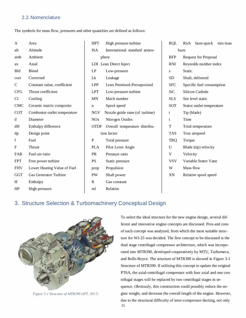
To select the ideal structure for the new engine design, several dif-
ferent and innovative engine concepts are discussed. Pros and cons
of each concept was analyzed, from which the most suitable struc-
ture for WJ-25 was decided. The first concept to be discussed is the
dual stage centrifugal compressor architecture, which was incorpo-
rated into MTR390, developed cooperatively by MTU, Turbomeca,
and Rolls-Royce. The structure of MTR390 is showed in Figure 3-1
Structure of MTR390. If utilizing this concept to update the original
PT6A, the axial-centrifugal compressor with four axial and one cen-
trifugal stages will be replaced by two centrifugal stages in se-
quence. Obviously, this construction could possibly reduce the en-
gine weight, and decrease the overall length of the engine. However,
due to the structural difficulty of inter-compressor ducting, not only Figure 3-1 Structure of MTR390 (IPT, 2017)
11
is it unusual to use more than two centrifugal stages in series, but the
highest PR achievable from two centrifugal stages is also limited to
15:1, since the pressure ratio of the second stage is likely designed
conservatively to compensate the extensive inter-stage flow turning
for avoiding massive separation (Walsh & Fletcher, 2004, p. 182).
A second possibility is the full-axial compressor architecture, which
is widely used in large turboprop engines, such as Europrop TP400.
The structure of Europrop TP400 is showed in Figure 3-2 Structure
of Europrop TP400. With all axial compressor stages, the overall
pressure ratio of the engine can reach a very high level, up to 25 or more. Higher overall pressure ratio enables higher cycle efficiency,
which in turn increases the aircraft flight range. However, to maintain a relatively satisfying compressor efficiency, more stages are
needed in a fully axial compression system in comparison with structural alternatives resembling PT6A. Due to the inverse relation-
ship between polytropic efficiency and stage loading (Glassman J. , 1992), stage work must be lowered to attain a higher polytropic
efficiency when a certain threshold for isentropic efficiency needs to be guaranteed. Thus, the disadvantage of increased engine weight
and length might be compromised by high overall PR. Additionally, axial compressors are predominantly favorable for turbomachin-
ery of mass flow rate larger than 10kg/s for aerospace applications (Walsh & Fletcher, 2004, p. 185). Small mass flow rate poses effi-
ciency challenges, such as the increased percentage tip clearance from the small blade size under constant manufacturing limits.
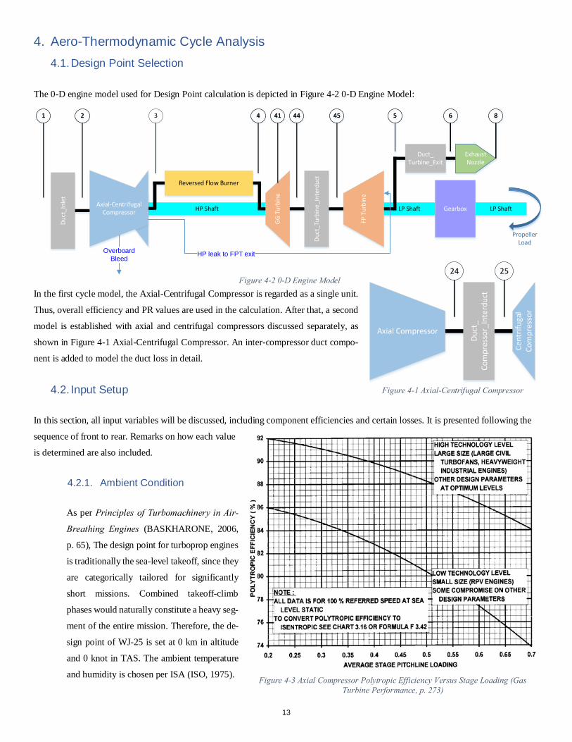
Coaxial contra-rotating is yet another concept proposed in the dis-
cussion. Contra-rotation is realized through a mechanism where two
mechanically independent rotors spin around a common axis, how-
ever, in opposite directions aiming for minimization of gyroscopic
effect. A typical structure of coaxial counterrotating turboprop en-
gine is Kuznetsov NK-62 shown in Figure 3-3 Structure of Kuz-
netsov NK-62 (Авиабаза, 2017). In coaxial counterrotating engines,
the propeller efficiency is increased by recovering tangential (rota-
tional) momentum from the leading propeller in its downstream
stage. Tangential velocity gradient in the downstream air doesn’t contribute to the thrust. Hence, conversion of airflow momentum
from tangential to axial increases both propeller efficiency and overall system effectiveness. But in engines of this kind, complex me-
chanical structure and sophisticated bearing systems are mandatory supplements for coaxial counterrotating spool configuration,
which are expensive in both fabrication and maintenance. Besides, the noise level of the engine is also dramatically increased by the
coaxial contra-rotating propeller. Therefore, synthesizing considerations on reliability and noise, the concept of NK-62 is not adopted.
After careful comparison and discussion, the original axial-centrifugal compressor with axial turbine and reverse-flow combustor
structure is finally chosen, whose feasibility has been validated in not only more than 30 years of PT6 development, but also in the
new emerging GE93 market disruptor. For WJ-25, this is the best combination for suitable overall pressure ratio, acceptable total
weight, and attainable technology readiness, regarding its mass flow rate, power level, and customer’s cost expectations.
Figure 3-3 Structure of Kuznetsov NK-62 (Авиабаза, 2017)
Figure 3-2 Structure of Europrop TP400 (Europrop, 2017)
12
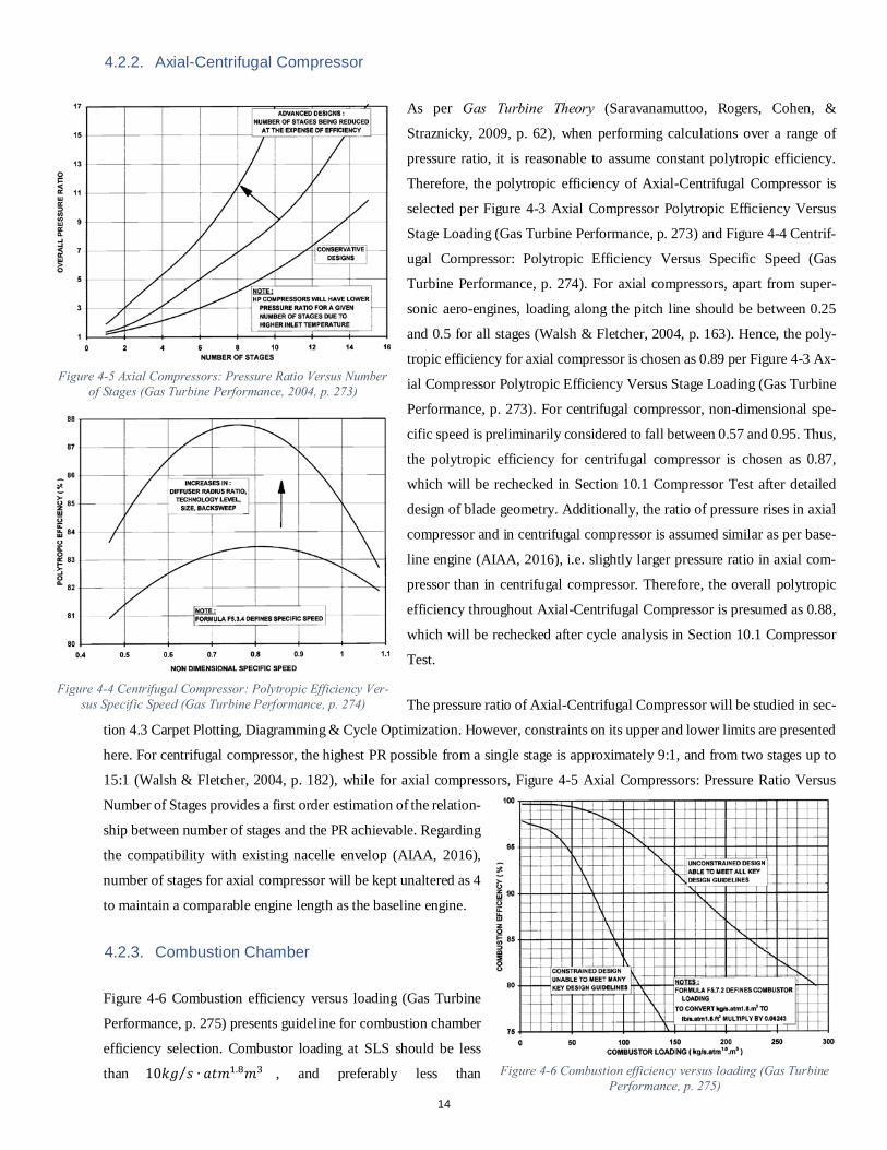
4. Aero-Thermodynamic Cycle Analysis4.1. Design Point Selection
The 0-D engine model used for Design Point calculation is depicted in Figure 4-2 0-D Engine Model:
In the first cycle model, the Axial-Centrifugal Compressor is regarded as a single unit.
Thus, overall efficiency and PR values are used in the calculation. After that, a second
model is established with axial and centrifugal compressors discussed separately, as
shown in Figure 4-1 Axial-Centrifugal Compressor. An inter-compressor duct compo-
nent is added to model the duct loss in detail.
4.2. Input Setup
In this section, all input variables will be discussed, including component efficiencies and certain losses. It is presented following the
sequence of front to rear. Remarks on how each value
is determined are also included.
4.2.1. Ambient Condition
As per Principles of Turbomachinery in Air-
Breathing Engines (BASKHARONE, 2006,
p. 65), The design point for turboprop engines
is traditionally the sea-level takeoff, since they
are categorically tailored for significantly
short missions. Combined takeoff-climb
phases would naturally constitute a heavy seg-
ment of the entire mission. Therefore, the de-
sign point of WJ-25 is set at 0 km in altitude
and 0 knot in TAS. The ambient temperature
and humidity is chosen per ISA (ISO, 1975).
HP Shaft
Duct
_Tur
bine
_Int
erdu
ct
Duct
_Inl
et
Exhaust Nozzle
Gearbox
Propeller Load
LP Shaft LP Shaft
Reversed Flow Burner
Axial-Centrifugal Compressor
GG T
urbi
ne
FP T
urbi
ne
Duct_Turbine_Exit
HP leak to FPT exit
321 4 41 44 45 5 6 821 4 41 44 45 5 6 8
OverboardBleed
Figure 4-2 0-D Engine Model
Figure 4-3 Axial Compressor Polytropic Efficiency Versus Stage Loading (Gas Turbine Performance, p. 273)
Figure 4-1 Axial-Centrifugal Compressor
Cent
rifug
alCo
mpr
esso
r
Axial Compressor
Duct
_Co
mpr
esso
r_In
terd
uct
2524
13
4.2.2. Axial-Centrifugal Compressor
As per Gas Turbine Theory (Saravanamuttoo, Rogers, Cohen, &
Straznicky, 2009, p. 62), when performing calculations over a range of
pressure ratio, it is reasonable to assume constant polytropic efficiency.
Therefore, the polytropic efficiency of Axial-Centrifugal Compressor is
selected per Figure 4-3 Axial Compressor Polytropic Efficiency Versus
Stage Loading (Gas Turbine Performance, p. 273) and Figure 4-4 Centrif-
ugal Compressor: Polytropic Efficiency Versus Specific Speed (Gas
Turbine Performance, p. 274). For axial compressors, apart from super-
sonic aero-engines, loading along the pitch line should be between 0.25
and 0.5 for all stages (Walsh & Fletcher, 2004, p. 163). Hence, the poly-
tropic efficiency for axial compressor is chosen as 0.89 per Figure 4-3 Ax-
ial Compressor Polytropic Efficiency Versus Stage Loading (Gas Turbine
Performance, p. 273). For centrifugal compressor, non-dimensional spe-
cific speed is preliminarily considered to fall between 0.57 and 0.95. Thus,
the polytropic efficiency for centrifugal compressor is chosen as 0.87,
which will be rechecked in Section 10.1 Compressor Test after detailed
design of blade geometry. Additionally, the ratio of pressure rises in axial
compressor and in centrifugal compressor is assumed similar as per base-
line engine (AIAA, 2016), i.e. slightly larger pressure ratio in axial com-
pressor than in centrifugal compressor. Therefore, the overall polytropic
efficiency throughout Axial-Centrifugal Compressor is presumed as 0.88,
which will be rechecked after cycle analysis in Section 10.1 Compressor
Test.
The pressure ratio of Axial-Centrifugal Compressor will be studied in sec-
tion 4.3 Carpet Plotting, Diagramming & Cycle Optimization. However, constraints on its upper and lower limits are presented
here. For centrifugal compressor, the highest PR possible from a single stage is approximately 9:1, and from two stages up to
15:1 (Walsh & Fletcher, 2004, p. 182), while for axial compressors, Figure 4-5 Axial Compressors: Pressure Ratio Versus
Number of Stages provides a first order estimation of the relation-
ship between number of stages and the PR achievable. Regarding
the compatibility with existing nacelle envelop (AIAA, 2016),
number of stages for axial compressor will be kept unaltered as 4
to maintain a comparable engine length as the baseline engine.
4.2.3. Combustion Chamber
Figure 4-6 Combustion efficiency versus loading (Gas Turbine
Performance, p. 275) presents guideline for combustion chamber
efficiency selection. Combustor loading at SLS should be less
than 10𝑘𝑘𝑘𝑘 𝑠𝑠 ∙ 𝑎𝑎𝑎𝑎𝑎𝑎1.8𝑎𝑎3⁄ , and preferably less than
Figure 4-4 Centrifugal Compressor: Polytropic Efficiency Ver-sus Specific Speed (Gas Turbine Performance, p. 274)
Figure 4-5 Axial Compressors: Pressure Ratio Versus Number of Stages (Gas Turbine Performance, 2004, p. 273)
Figure 4-6 Combustion efficiency versus loading (Gas Turbine Performance, p. 275)
14
5𝑘𝑘𝑘𝑘 𝑠𝑠 ∙ 𝑎𝑎𝑎𝑎𝑎𝑎1.8𝑎𝑎3⁄ (Walsh & Fletcher, 2004, p. 195). Therefore, combustion chamber efficiency is chosen as 0.995. The com-
bustor cold pressure loss is usually between 2 and 4% of total pressure at the design point, while fundamental loss around 0.05%
and 0.15% (Walsh & Fletcher, 2004, p. 194). Thus, combustor pressure ratio is chosen as 0.975, which counts for 4% of losses.
Combustor exit temperature is mainly restricted by the material of turbine stators and rotors. With new emergence of CMC,
this design incorporates CMC for all turbine nozzles, blades, and discs. The use of CMC in engine hot section greatly improves
COT, reduces weight, and eliminates the need for sophisticated turbine cooling. The SiC CMC with a highest working temper-
ature of 2400°𝐹𝐹/1316°𝐶𝐶 (Wood, 2013) has already been made into engine service by GE Aviation (Norris, 2015), while other
types of CMC with more aggressive high-temp capabilities are still under research and development. Additionally, a combustor
exit temperature profile parameter, OTDF, should be controlled to less than 50% and ideally less than 20% (Walsh & Fletcher,
2004, p. 198). Thus, to tolerate reasonable level of combustor outlet temperature unevenness, i.e. a no less than 20% OTDF,
the combustor exit temperature, i.e. COT, should be lower than the highest material capability to ease the design challenge of
combustor exit mixing, and will be studied in detail in section
4.3 Carpet Plotting, Diagramming & Cycle Optimization.
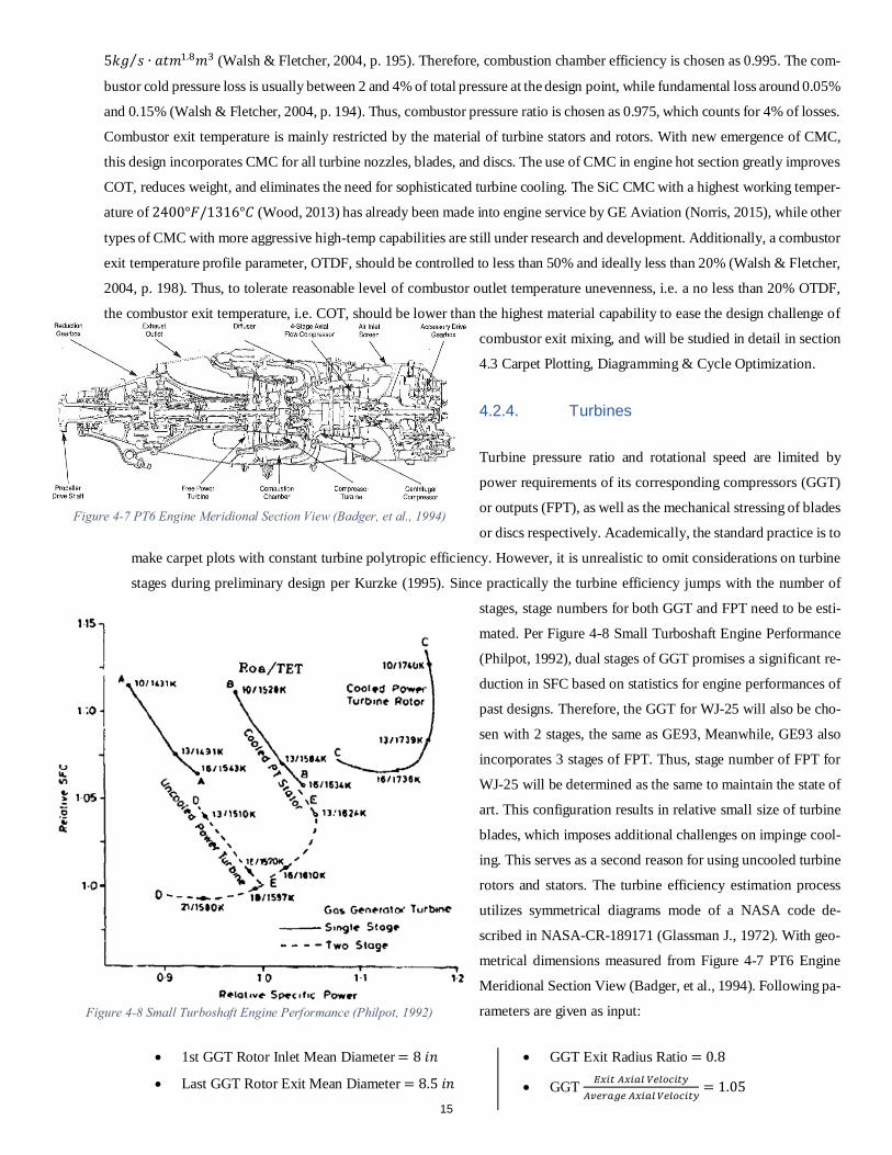
4.2.4. Turbines
Turbine pressure ratio and rotational speed are limited by
power requirements of its corresponding compressors (GGT)
or outputs (FPT), as well as the mechanical stressing of blades
or discs respectively. Academically, the standard practice is to
make carpet plots with constant turbine polytropic efficiency. However, it is unrealistic to omit considerations on turbine
stages during preliminary design per Kurzke (1995). Since practically the turbine efficiency jumps with the number of
stages, stage numbers for both GGT and FPT need to be esti-
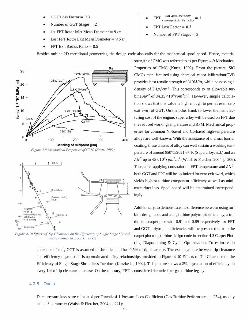
mated. Per Figure 4-8 Small Turboshaft Engine Performance
(Philpot, 1992), dual stages of GGT promises a significant re-
duction in SFC based on statistics for engine performances of
past designs. Therefore, the GGT for WJ-25 will also be cho-
sen with 2 stages, the same as GE93, Meanwhile, GE93 also
incorporates 3 stages of FPT. Thus, stage number of FPT for
WJ-25 will be determined as the same to maintain the state of
art. This configuration results in relative small size of turbine
blades, which imposes additional challenges on impinge cool-
ing. This serves as a second reason for using uncooled turbine
rotors and stators. The turbine efficiency estimation process
utilizes symmetrical diagrams mode of a NASA code de-
scribed in NASA-CR-189171 (Glassman J., 1972). With geo-
metrical dimensions measured from Figure 4-7 PT6 Engine
Meridional Section View (Badger, et al., 1994). Following pa-
rameters are given as input:
• 1st GGT Rotor Inlet Mean Diameter = 8 𝑖𝑖𝑠𝑠
• Last GGT Rotor Exit Mean Diameter = 8.5 𝑖𝑖𝑠𝑠
• GGT Exit Radius Ratio = 0.8
• GGT 𝐸𝐸𝐸𝐸𝐸𝐸𝐸𝐸 𝐴𝐴𝐸𝐸𝐸𝐸𝐴𝐴𝐴𝐴 𝑉𝑉𝑉𝑉𝐴𝐴𝑉𝑉𝑉𝑉𝐸𝐸𝐸𝐸𝑉𝑉𝐴𝐴𝐴𝐴𝑉𝑉𝐴𝐴𝐴𝐴𝐴𝐴𝑉𝑉 𝐴𝐴𝐸𝐸𝐸𝐸𝐴𝐴𝐴𝐴 𝑉𝑉𝑉𝑉𝐴𝐴𝑉𝑉𝑉𝑉𝐸𝐸𝐸𝐸𝑉𝑉
= 1.05
Figure 4-7 PT6 Engine Meridional Section View (Badger, et al., 1994)
Figure 4-8 Small Turboshaft Engine Performance (Philpot, 1992)
15
• GGT Loss Factor = 0.3
• Number of GGT Stages = 2
• 1st FPT Rotor Inlet Mean Diameter = 9 𝑖𝑖𝑠𝑠
• Last FPT Rotor Exit Mean Diameter = 9.5 𝑖𝑖𝑠𝑠
• FPT Exit Radius Ratio = 0.5
• FPT 𝐸𝐸𝐸𝐸𝐸𝐸𝐸𝐸 𝐴𝐴𝐸𝐸𝐸𝐸𝐴𝐴𝐴𝐴 𝑉𝑉𝑉𝑉𝐴𝐴𝑉𝑉𝑉𝑉𝐸𝐸𝐸𝐸𝑉𝑉𝐴𝐴𝐴𝐴𝑉𝑉𝐴𝐴𝐴𝐴𝐴𝐴𝑉𝑉 𝐴𝐴𝐸𝐸𝐸𝐸𝐴𝐴𝐴𝐴 𝑉𝑉𝑉𝑉𝐴𝐴𝑉𝑉𝑉𝑉𝐸𝐸𝐸𝐸𝑉𝑉
= 1
• FPT Loss Factor = 0.3
• Number of FPT Stages = 3
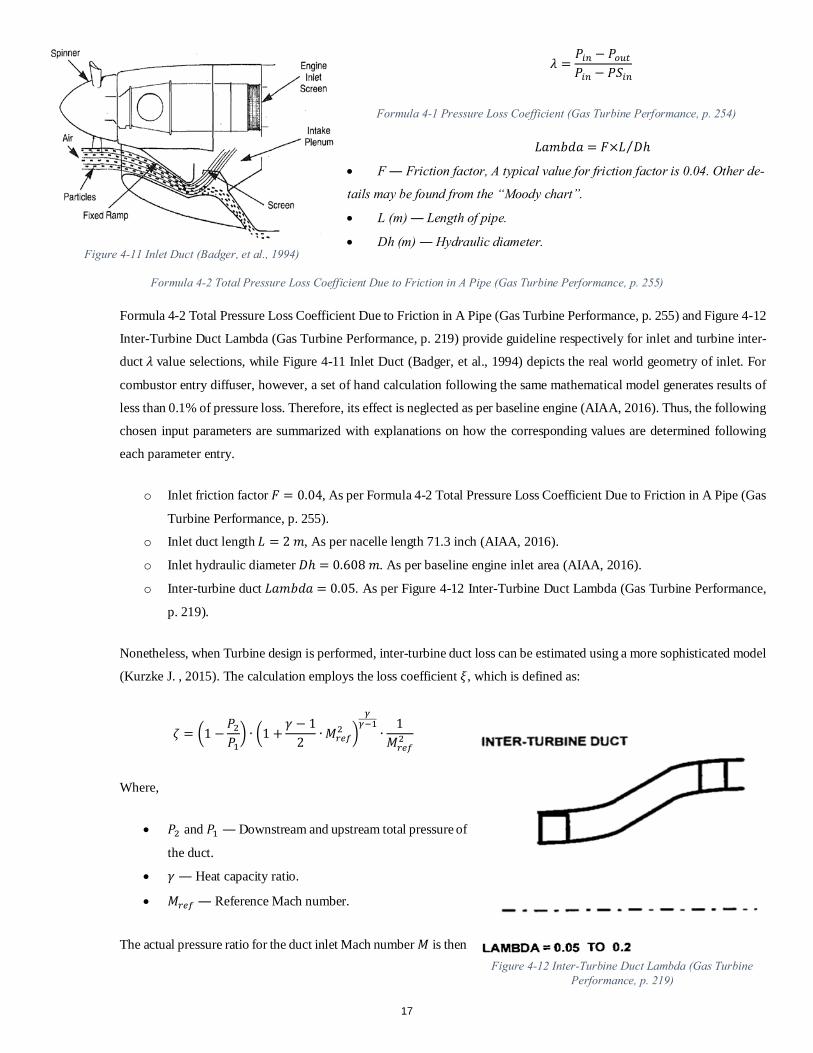
Besides turbine 2D meridional geometries, the design code also calls for the mechanical spool speed. Hence, material
strength of CMC was referred to as per Figure 4-9 Mechanical
Properties of CMC (Kurtz, 1992). From the picture, SiC
CMCs manufactured using chemical vapor infiltration(CVI)
provides best tensile strength of 310𝑀𝑀𝑃𝑃𝑎𝑎, while possessing a
density of 2.1𝑘𝑘 𝑠𝑠𝑎𝑎3⁄ . This corresponds to an allowable tur-
bine 𝐴𝐴𝑁𝑁2 of 84.35×10⁶𝑟𝑟𝑝𝑝𝑎𝑎2𝑎𝑎2. However, simple calcula-
tion shows that this value is high enough to permit even zero
exit swirl of GGT. On the other hand, to lower the manufac-
turing cost of the engine, super alloy will be used on FPT due
the reduced working temperature and RPM. Mechanical prop-
erties for common Ni-based and Co-based high-temperature
alloys are well-known. With the assistance of thermal barrier
coating, these classes of alloy can well sustain a working tem-
perature of around 850ºC/2021.67°R (Superalloy, n.d.) and an
𝐴𝐴𝑁𝑁2 up to 45×106𝑟𝑟𝑝𝑝𝑎𝑎2𝑎𝑎2 (Walsh & Fletcher, 2004, p. 206).
Thus, after applying constraint on FPT temperature and 𝐴𝐴𝑁𝑁2,
both GGT and FPT will be optimized for zero exit swirl, which
yields highest turbine component efficiency as well as mini-
mum duct loss. Spool speed will be determined correspond-
ingly.
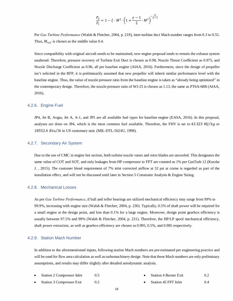
Additionally, to demonstrate the difference between using tur-
bine design code and using turbine polytropic efficiency, a tra-
ditional carpet plot with 0.91 and 0.89 respectively for FPT
and GGT polytropic efficiencies will be presented next to the
carpet plot uing turbine design code in section 4.3 Carpet Plot-
ting, Diagramming & Cycle Optimization. To estimate tip
clearance effects, GGT is assumed unshrouded and has 0.5% of tip clearance. The exchange rate between tip clearance
and efficiency degradation is approximated using relationships provided in Figure 4-10 Effects of Tip Clearance on the
Efficiency of Single Stage Shroudless Turbines (Kurzke J. , 1992). This picture shows a 2% degradation of efficiency on
every 1% of tip clearance increase. On the contrary, FPT is considered shrouded per gas turbine legacy.
4.2.5. Ducts
Duct pressure losses are calculated per Formula 4-1 Pressure Loss Coefficient (Gas Turbine Performance, p. 254), usually
called 𝜆𝜆 parameter (Walsh & Fletcher, 2004, p. 221):
Figure 4-10 Effects of Tip Clearance on the Efficiency of Single Stage Shroud-less Turbines (Kurzke J. , 1992)
Figure 4-9 Mechanical Properties of CMC (Kurtz, 1992)
16
𝜆𝜆 =𝑃𝑃𝐸𝐸𝑖𝑖 − 𝑃𝑃𝑉𝑉𝑜𝑜𝐸𝐸𝑃𝑃𝐸𝐸𝑖𝑖 − 𝑃𝑃𝑆𝑆𝐸𝐸𝑖𝑖
Formula 4-1 Pressure Loss Coefficient (Gas Turbine Performance, p. 254)
𝐿𝐿𝑎𝑎𝑎𝑎𝑙𝑙𝑠𝑠𝑎𝑎 = 𝐹𝐹×𝐿𝐿 𝐷𝐷ℎ⁄
• F ― Friction factor, A typical value for friction factor is 0.04. Other de-
tails may be found from the “Moody chart”.
• L (m) ― Length of pipe.
• Dh (m) ― Hydraulic diameter.
Formula 4-2 Total Pressure Loss Coefficient Due to Friction in A Pipe (Gas Turbine Performance, p. 255)
Formula 4-2 Total Pressure Loss Coefficient Due to Friction in A Pipe (Gas Turbine Performance, p. 255) and Figure 4-12
Inter-Turbine Duct Lambda (Gas Turbine Performance, p. 219) provide guideline respectively for inlet and turbine inter-
duct 𝜆𝜆 value selections, while Figure 4-11 Inlet Duct (Badger, et al., 1994) depicts the real world geometry of inlet. For
combustor entry diffuser, however, a set of hand calculation following the same mathematical model generates results of
less than 0.1% of pressure loss. Therefore, its effect is neglected as per baseline engine (AIAA, 2016). Thus, the following
chosen input parameters are summarized with explanations on how the corresponding values are determined following
each parameter entry.
o Inlet friction factor 𝐹𝐹 = 0.04, As per Formula 4-2 Total Pressure Loss Coefficient Due to Friction in A Pipe (Gas
Turbine Performance, p. 255).
o Inlet duct length 𝐿𝐿 = 2 𝑎𝑎, As per nacelle length 71.3 inch (AIAA, 2016).
o Inlet hydraulic diameter 𝐷𝐷ℎ = 0.608 𝑎𝑎. As per baseline engine inlet area (AIAA, 2016).
o Inter-turbine duct 𝐿𝐿𝑎𝑎𝑎𝑎𝑙𝑙𝑠𝑠𝑎𝑎 = 0.05. As per Figure 4-12 Inter-Turbine Duct Lambda (Gas Turbine Performance,
p. 219).
Nonetheless, when Turbine design is performed, inter-turbine duct loss can be estimated using a more sophisticated model
(Kurzke J. , 2015). The calculation employs the loss coefficient 𝜉𝜉, which is defined as:
𝜁𝜁 = �1 −𝑃𝑃2𝑃𝑃1� ∙ �1 +
𝛾𝛾 − 12 ∙ 𝑀𝑀𝐴𝐴𝑉𝑉𝑟𝑟
2 �𝛾𝛾
𝛾𝛾−1∙
1𝑀𝑀𝐴𝐴𝑉𝑉𝑟𝑟
2
Where,
• 𝑃𝑃2 and 𝑃𝑃1 ― Downstream and upstream total pressure of
the duct.
• 𝛾𝛾 ― Heat capacity ratio.
• 𝑀𝑀𝐴𝐴𝑉𝑉𝑟𝑟 ― Reference Mach number.
The actual pressure ratio for the duct inlet Mach number 𝑀𝑀 is then Figure 4-12 Inter-Turbine Duct Lambda (Gas Turbine
Performance, p. 219)
Figure 4-11 Inlet Duct (Badger, et al., 1994)
17
𝑃𝑃2𝑃𝑃1
= 1− 𝜉𝜉 ∙ 𝑀𝑀2 ∙ �1 +𝛾𝛾 − 1
2 ∙ 𝑀𝑀2�− 𝛾𝛾𝛾𝛾−1
Per Gas Turbine Performance (Walsh & Fletcher, 2004, p. 219), inter-turbine duct Mach number ranges from 0.3 to 0.55.
Thus, 𝑀𝑀𝐴𝐴𝑉𝑉𝑟𝑟 is chosen as the middle value 0.4.
Since compatibility with original aircraft needs to be maintained, new engine proposal tends to remain the exhaust system
unaltered. Therefore, pressure recovery of Turbine Exit Duct is chosen as 0.98, Nozzle Thrust Coefficient as 0.975, and
Nozzle Discharge Coefficient as 0.96, all per baseline engine (AIAA, 2016). Furthermore, since the design of propeller
isn’t solicited in the RFP, it is preliminarily assumed that new propeller will inherit similar performance level with the
baseline engine. Thus, the value of nozzle pressure ratio from the baseline engine is taken as “already being optimized” in
the contemporary design. Therefore, the nozzle pressure ratio of WJ-25 is chosen as 1.13, the same as PT6A-68B (AIAA,
2016).
4.2.6. Engine Fuel
JP4, Jet B, Avgas, Jet A, A-1, and JP5 are all available fuel types for baseline engine (EASA, 2016). In this proposal,
analyses are done on JP4, which is the most common fuel available. Therefore, the FHV is set to 43.323 𝑀𝑀𝑀𝑀 𝑘𝑘𝑘𝑘⁄ or
18552.4 𝐵𝐵𝑎𝑎𝐵𝐵 𝑙𝑙𝑙𝑙⁄ in US customary unit. (MIL-DTL-5624U, 1998).
4.2.7. Secondary Air System
Due to the use of CMC in engine hot section, both turbine nozzle vanes and rotor blades are uncooled. This designates the
same value of COT and SOT, and only leakages from HP compressor to FPT are counted as 1% per GasTurb 12 (Kurzke
J. , 2015). The customer bleed requirement of 7% inlet corrected airflow at 32 psi at cruise is regarded as part of the
installation effect, and will not be discussed until later in Section 5 Constraint Analysis & Engine Sizing.
4.2.8. Mechanical Losses
As per Gas Turbine Performance, if ball and roller bearings are utilized mechanical efficiency may range from 99% to
99.9%, increasing with engine size (Walsh & Fletcher, 2004, p. 230). Typically, 0.5% of shaft power will be required for
a small engine at the design point, and less than 0.1% for a large engine. Moreover, design point gearbox efficiency is
usually between 97.5% and 99% (Walsh & Fletcher, 2004, p. 231). Therefore, the HP/LP spool mechanical efficiency,
shaft power extraction, as well as gearbox efficiency are chosen as 0.995, 0.5%, and 0.985 respectively.
4.2.9. Station Mach Number
In addition to the aforementioned inputs, following station Mach numbers are pre-estimated per engineering practice and
will be used for flow area calculation as well as turbomachinery design. Note that these Mach numbers are only preliminary
assumptions, and results may differ slightly after detailed aerodynamic analysis.
• Station 2 Compressor Inlet 0.5
• Station 3 Compressor Exit 0.2
• Station 4 Burner Exit 0.2
• Station 45 FPT Inlet 0.4
18
• Station 6 Turbine Exit Duct Exit 0.2 • Other Stations by Turbine Design Code
4.2.10. Input Summary
Table 4-1 Summary of Fixed Input Parameters provides a tabular view of all constant inputs for design point aero-thermo-
dynamic calculation. Parameters proprietary to Axial-Centrifugal Compressor only, to Installation Effects only, and to
carpet plot without turbine design only are highlighted in orange, green, and blue respectively. Effects of small variation
of these parameters on engine performance will be discussed in Section 6 Cycle Summary.
1 Parameters marked green are for Installation Effects only.
2 Parameters marked blue are for conventional carpet plot without turbine design only.
Type Parameters Value Type Parameters Value
Compressors
Compressor overall polytropic efficiency 0.88 Combustor
Combustor Efficiency 0.995
Centrifugal compressor polytropic effi-
ciency 0.87
Combustor Pressure ratio 0.975
Ducts
Inlet friction factor1 0.04
Axial compressor polytropic efficiency 0.89 Inlet duct length (m) 2
Turbines
GGT polytropic efficiency2 0.89 Inlet hydraulic diameter (m) 0.608
1st GGT Rotor Inlet Mean Diameter 8 Inter-turbine duct 𝜆𝜆 0.05
Last GGT Rotor Exit Mean Diameter (in) 8.5 Turbine exit duct pressure ratio 0.98
GGT Exit Radius Ratio 0.8 Nozzle thrust coefficient 0.975
GGT 𝐸𝐸𝐸𝐸𝐸𝐸𝐸𝐸 𝐴𝐴𝐸𝐸𝐸𝐸𝐴𝐴𝐴𝐴 𝑉𝑉𝑉𝑉𝐴𝐴𝑉𝑉𝑉𝑉𝐸𝐸𝐸𝐸𝑉𝑉𝐴𝐴𝐴𝐴𝑉𝑉𝐴𝐴𝐴𝐴𝐴𝐴𝑉𝑉 𝐴𝐴𝐸𝐸𝐸𝐸𝐴𝐴𝐴𝐴 𝑉𝑉𝑉𝑉𝐴𝐴𝑉𝑉𝑉𝑉𝐸𝐸𝐸𝐸𝑉𝑉 1.05 Nozzle pressure ratio 1.13
GGT Loss Factor 0.3 Nozzle discharge coefficient 0.96
Number of GGT Stages 2 Inter-turbine duct 𝑀𝑀𝐴𝐴𝑉𝑉𝑟𝑟 0.4
GGT Exit Swirl (°) 0 Engine
Fuel
FHV (𝑀𝑀𝑀𝑀 𝑘𝑘𝑘𝑘⁄ ) 43.323
GGT percentage tip clearance (%) 0.5 FHV (𝐵𝐵𝑎𝑎𝐵𝐵 𝑙𝑙𝑙𝑙⁄ ) 18552,4
FPT polytropic efficiency 0.91 Secondary
Air System
leakages from HP compressor
to FPT 1%
1st FPT Rotor Inlet Mean Diameter (in) 9
Last FPT Rotor Exit Mean Diameter (in) 9.5
Mechanical
losses
HP Mechanical efficiency 0.995
FPT Exit Radius Ratio (in) 0.5 LP Mechanical efficiency 0.995
FPT 𝐸𝐸𝐸𝐸𝐸𝐸𝐸𝐸 𝐴𝐴𝐸𝐸𝐸𝐸𝐴𝐴𝐴𝐴 𝑉𝑉𝑉𝑉𝐴𝐴𝑉𝑉𝑉𝑉𝐸𝐸𝐸𝐸𝑉𝑉𝐴𝐴𝐴𝐴𝑉𝑉𝐴𝐴𝐴𝐴𝐴𝐴𝑉𝑉 𝐴𝐴𝐸𝐸𝐸𝐸𝐴𝐴𝐴𝐴 𝑉𝑉𝑉𝑉𝐴𝐴𝑉𝑉𝑉𝑉𝐸𝐸𝐸𝐸𝑉𝑉 1 Shaft power extraction 0.5%
FPT Loss Factor 0.3 Gearbox efficiency 0.985
Number of FPT Stages 3
Station
Mach
Number
Station 2 Compressor Inlet 0.5
FPT Exit Swirl (°) 0 Station 3 Compressor Exit 0.2
% Efficiency change/% Tip clearance 2 Station 4 Burner Exit 0.2
Ambient
Altitude (km/ft.) 0 Station 45 FPT Inlet 0.4
TAS (knot/Mach) 0 Station 6 Turbine Exit Duct
Exit 0.2
Conditions ISA
Table 4-1 Summary of Fixed Input Parameters
19
Parameters to be studied in following sections as well as their constraints include:
1. Overall PR Constraints: engine length and weight
2. Axial Compressor PR Per Figure 4-5 Axial Compressors: Pressure Ratio Versus Number of Stages
3. Centrifugal Compressor PR Constraints: no more than 9:1 for a single stage
4. T4, namely COT Constraints: OTDF larger than 20%
5. Inlet corrected mass flow rate To be calculated per power requirements in Section 5.7 Engine Sizing.
4.3. Carpet Plotting, Diagramming & Cycle Optimization
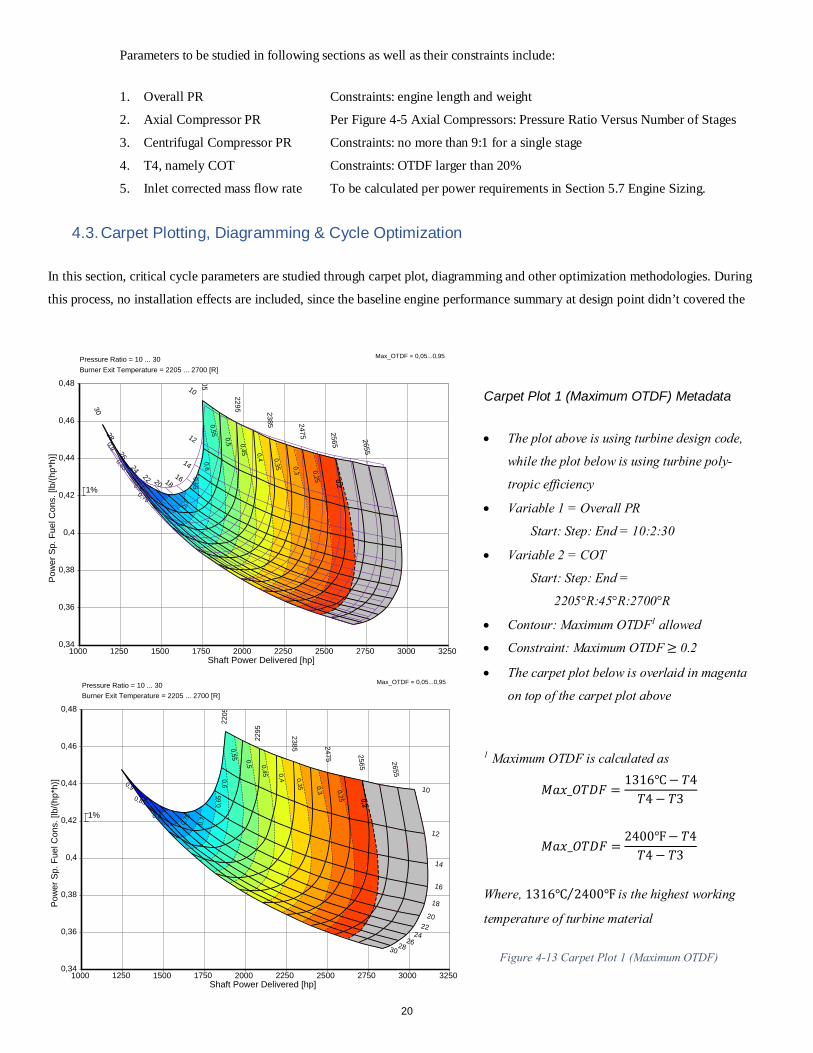
In this section, critical cycle parameters are studied through carpet plot, diagramming and other optimization methodologies. During
this process, no installation effects are included, since the baseline engine performance summary at design point didn’t covered the
Carpet Plot 1 (Maximum OTDF) Metadata
• The plot above is using turbine design code,
while the plot below is using turbine poly-
tropic efficiency
• Variable 1 = Overall PR
Start: Step: End = 10:2:30
• Variable 2 = COT
Start: Step: End =
2205°R:45°R:2700°R
• Contour: Maximum OTDF1 allowed
• Constraint: Maximum OTDF ≥ 0.2
• The carpet plot below is overlaid in magenta
on top of the carpet plot above
1 Maximum OTDF is calculated as
𝑀𝑀𝑎𝑎𝑀𝑀_𝑂𝑂𝑂𝑂𝐷𝐷𝐹𝐹 =1316℃− 𝑂𝑂4𝑂𝑂4− 𝑂𝑂3
𝑀𝑀𝑎𝑎𝑀𝑀_𝑂𝑂𝑂𝑂𝐷𝐷𝐹𝐹 =2400℉− 𝑂𝑂4𝑂𝑂4− 𝑂𝑂3
Where, 1316℃ 2400℉⁄ is the highest working
temperature of turbine material
Figure 4-13 Carpet Plot 1 (Maximum OTDF) 1000 1250 1500 1750 2000 2250 2500 2750 3000 3250
Shaft Power Delivered [hp]
0,34
0,36
0,38
0,4
0,42
0,44
0,46
0,48
Pow
er S
p. F
uel C
ons.
[lb/
(hp*
h)]
Pressure Ratio = 10 ... 30 Burner Exit Temperature = 2205 ... 2700 [R]
Max_OTDF = 0,05...0,95
0,1
0,15
0,2
0,25
0,3
0,35
0,4
0,45
0,5
0,550,6
0,65
0,7
0,750,8
0,85
0,9
0,2
2205
2295 2385 2475 2565 2655
10
12
14
16
18
2022
24262830
1%
1000 1250 1500 1750 2000 2250 2500 2750 3000 3250Shaft Power Delivered [hp]
0,34
0,36
0,38
0,4
0,42
0,44
0,46
0,48
Pow
er S
p. F
uel C
ons.
[lb/
(hp*
h)]
Pressure Ratio = 10 ... 30 Burner Exit Temperature = 2205 ... 2700 [R]
Max_OTDF = 0,05...0,95
0,1
0,15
0,2
0,25
0,3
0,35
0,4
0,45
0,5
0,550,6
0,65
0,7
0,75
0,8
0,85
0,9
0,2
05
2295 2385 2475 2565 2655
10
12
14161820
22
24
26
28
30
1%
20
airframe influences when provided in the RFP. Therefore, zero inlet loss, no power offtake, and absence of customer bleed are consid-
ered when carpet plotting for design point analysis, as were in the engine summary table from Request for Proposal (AIAA, 2016).
From Figure 4-13 Carpet Plot 1 (Maximum OTDF), it is easy to
detect the limiting effect of OTDF on COT. When acceptable
OTDF is necessary at all operating conditions of various engine
PRs, the highest COT usable is restricted to around
1425K/2565°R, which provides reasonable tolerance to manu-
facturing errors and engine deterioration. In the retrospect, Fig-
ure 4-15 Carpet Plot 2 (Thermal Efficiency) provides the insight
that, when pursuing higher engine thermal efficiency, designers
should push the operating point as much as possible to the top
right corner, where both elevated COT and increased PR are be-
ing indicated. Furthermore, this carplot plot also demonstrate
that GGT PR is more directly affected by the compressor PR
and less sensitive to COT, while FPT PR is a function of both
variables. Commonly, the PR upper limit of a highly loaded
single-stage turbine is around 4. Thus, the highest PRs on the
plot, around 4.2 and 11 for GGT and FPT respectively, are both
achievable from 2 stages of GGT and 3 stages of FPT.
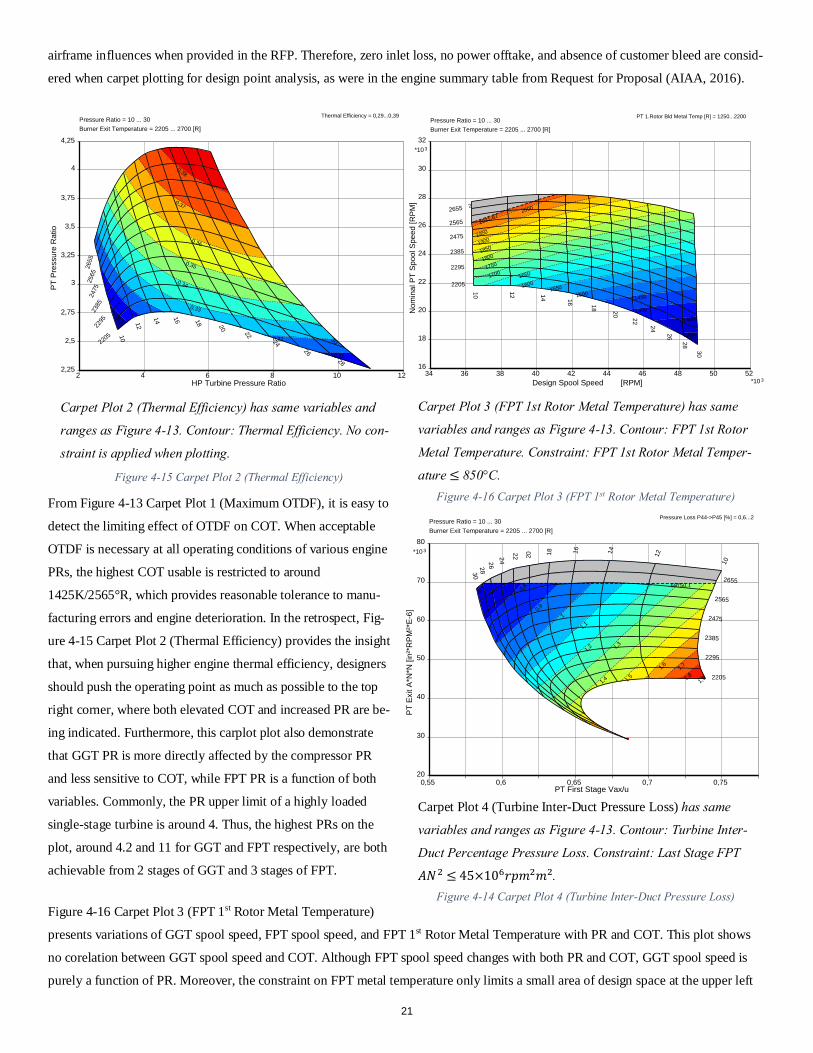
Figure 4-16 Carpet Plot 3 (FPT 1st Rotor Metal Temperature)
presents variations of GGT spool speed, FPT spool speed, and FPT 1st Rotor Metal Temperature with PR and COT. This plot shows
no corelation between GGT spool speed and COT. Although FPT spool speed changes with both PR and COT, GGT spool speed is
purely a function of PR. Moreover, the constraint on FPT metal temperature only limits a small area of design space at the upper left
Carpet Plot 2 (Thermal Efficiency) has same variables and
ranges as Figure 4-13. Contour: Thermal Efficiency. No con-
straint is applied when plotting.
Figure 4-15 Carpet Plot 2 (Thermal Efficiency)
2 4 6 8 10 12HP Turbine Pressure Ratio
2,25
2,5
2,75
3
3,25
3,5
3,75
4
4,25
PT P
ress
ure
Rat
io
Pressure Ratio = 10 ... 30 Burner Exit Temperature = 2205 ... 2700 [R]
Thermal Efficiency = 0,29...0,39
0,3
0,31
0,32
0,33
0,34
0,35
0,36
0,37
0,38
2205
2295
2385
2475
2565
2655
10
12
14 16 18 20 22
24
26
28
30
Carpet Plot 3 (FPT 1st Rotor Metal Temperature) has same
variables and ranges as Figure 4-13. Contour: FPT 1st Rotor
Metal Temperature. Constraint: FPT 1st Rotor Metal Temper-
ature ≤ 850°C. Figure 4-16 Carpet Plot 3 (FPT 1st Rotor Metal Temperature)
34 36 38 40 42 44 46 48 50 52*10 3Design Spool Speed [RPM]
16
18
20
22
24
26
28
30
32*10 3
Nom
inal
PT
Spoo
l Spe
ed [R
PM]
Pressure Ratio = 10 ... 30 Burner Exit Temperature = 2205 ... 2700 [R]
PT 1.Rotor Bld Metal Temp [R] = 1250...2200
1300
13501400
1450150015501600
165017001750
18001850
19001950
20002050
21002150
2021,67
2205
2295
2385
2475
2565
2655
10 12 14 16 18 20 22 24
26
28
30
Carpet Plot 4 (Turbine Inter-Duct Pressure Loss) has same
variables and ranges as Figure 4-13. Contour: Turbine Inter-
Duct Percentage Pressure Loss. Constraint: Last Stage FPT
𝐴𝐴𝑁𝑁2 ≤ 45×106𝑟𝑟𝑝𝑝𝑎𝑎2𝑎𝑎2.
0,55 0,6 0,65 0,7 0,75PT First Stage Vax/u
20
30
40
50
60
70
80*10 3
PT E
xit A
*N*N
[in²
*RPM
²*E-
6]
Pressure Ratio = 10 ... 30 Burner Exit Temperature = 2205 ... 2700 [R]
Pressure Loss P44->P45 [%] = 0,6...2
0,7 0,8
0,9
1
1,1
1,2 1,3
1,4 1,51,6 1,7
1,81,9
69750,1
2205
2295
2385
2475
2565
2655
10
1214161820
2224262830
Figure 4-14 Carpet Plot 4 (Turbine Inter-Duct Pressure Loss)
21
corner. On the other hand, Figure 4-14 Carpet Plot 4 (Turbine Inter-Duct Pressure Loss) demonstrates the relationship between, FPT
first stage flow coefficient, FPT last stage 𝐴𝐴𝑁𝑁2, inter-turbine duct pressure loss and PR, COT. FPT last stage 𝐴𝐴𝑁𝑁2 is purely a function
of FPT spool speed, while inter-turbine duct pressure loss is only related to duct Mach number. From the plot, both FPT first stage
flow coefficient (below 0.75) and inter-turbine duct pressure loss (below 2%) are satisfactory on all design spaces. Thus, no
constraints were applied to them. Nevertheless, the highest value for FPT last stage 𝐴𝐴𝑁𝑁2 approachs 50×106𝑟𝑟𝑝𝑝𝑎𝑎2𝑎𝑎2 on the high COT
end. Therefore, a constraint was put on to limit its blade stress.
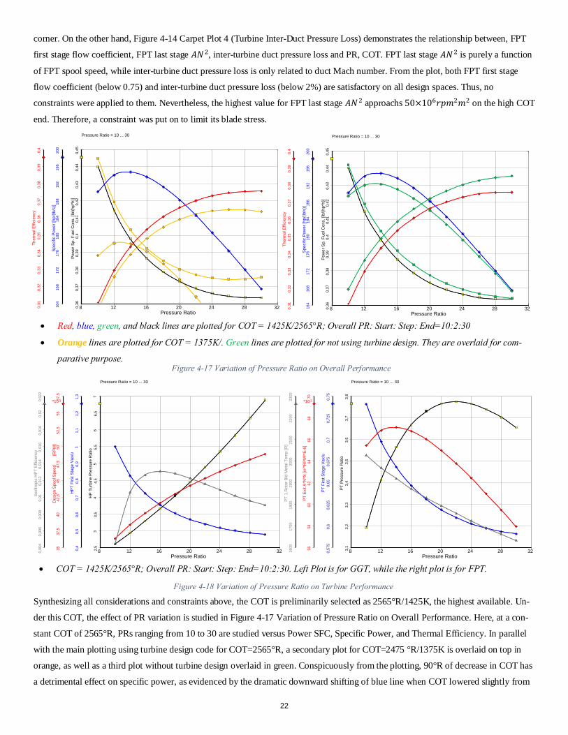
Synthesizing all considerations and constraints above, the COT is preliminarily selected as 2565°R/1425K, the highest available. Un-
der this COT, the effect of PR variation is studied in Figure 4-17 Variation of Pressure Ratio on Overall Performance. Here, at a con-
stant COT of 2565°R, PRs ranging from 10 to 30 are studied versus Power SFC, Specific Power, and Thermal Efficiency. In parallel
with the main plotting using turbine design code for COT=2565°R, a secondary plot for COT=2475 °R/1375K is overlaid on top in
orange, as well as a third plot without turbine design overlaid in green. Conspicuously from the plotting, 90°R of decrease in COT has
a detrimental effect on specific power, as evidenced by the dramatic downward shifting of blue line when COT lowered slightly from
Figure 4-17 Variation of Pressure Ratio on Overall Performance
• Red, blue, green, and black lines are plotted for COT = 1425K/2565°R; Overall PR: Start: Step: End=10:2:30
• Orange lines are plotted for COT = 1375K/. Green lines are plotted for not using turbine design. They are overlaid for com-
parative purpose.
8 12 16 20 24 28 32Pressure Ratio
0,36
0,37
0,38
0,39
0,4
0,41
0,42
0,43
0,44
0,45
Pow
er S
p. F
uel C
ons.
[lb/
(hp*
h)]
164
168
172
176
180
184
188
192
196
200
Spec
ific
Pow
er [h
p/(lb
/s)]
0,31
0,32
0,33
0,34
0,35
0,36
0,37
0,38
0,39
0,4
Ther
mal
Effi
cien
cy
Pressure Ratio = 10 ... 30
8 12 16 20 24 28 32Pressure Ratio
0,36
0,37
0,38
0,39
0,4
0,41
0,42
0,43
0,44
0,45
Pow
er S
p. F
uel C
ons.
[lb/
(hp*
h)]
164
168
172
176
180
184
188
192
196
200
Spec
ific
Pow
er [h
p/(lb
/s)]
0,31
0,32
0,33
0,34
0,35
0,36
0,37
0,38
0,39
0,4
Ther
mal
Effi
cien
cy
Pressure Ratio = 10 ... 30
8 12 16 20 24 28 32Pressure Ratio
2,5
33,
54
4,5
55,
56
6,5
7H
P Tu
rbin
e Pr
essu
re R
atio
0,4
0,5
0,6
0,7
0,8
0,9
11,
11,
21,
3H
PT F
irst S
tage
Vax
/u
3537
,540
42,5
4547
,550
52,5
5557
,5
*10 3
Des
ign
Spoo
l Spe
ed
[
RPM
]
0,90
40,
906
0,90
80,
910,
912
0,91
40,
916
0,91
80,
920,
922
Isen
tropi
c H
PT E
ffici
ency
Pressure Ratio = 10 ... 30
8 12 16 20 24 28 32Pressure Ratio
3,1
3,2
3,3
3,4
3,5
3,6
3,7
3,8
PT P
ress
ure
Rat
io
0,57
50,
60,
625
0,65
0,67
50,
70,
725
0,75
PT F
irst S
tage
Vax
/u
5658
6062
6466
6870
*10 3
PT E
xit A
*N*N
[in²
*RPM
²*E-
6]
1600
1700
1800
1900
2000
2100
2200
2300
PT 1
.Rot
or B
ld M
etal
Tem
p [R
]
Pressure Ratio = 10 ... 30
Figure 4-18 Variation of Pressure Ratio on Turbine Performance
• COT = 1425K/2565°R; Overall PR: Start: Step: End=10:2:30. Left Plot is for GGT, while the right plot is for FPT.
22
2565°R to 2475°R. Additionally, higher COT also gently improves SFC and Thermal Efficiency, since with increased cycle energy,
percentage loss decreases when absolute losses remain relatively unchanged.
Besides the study on engine overall performance, effect of overall PR on turbine performance is also plotted in Figure 4-18 Variation
of Pressure Ratio on Turbine Performance. Evidently from the diagram, flow coefficients for both GGT and FPT decrease with overall
PR, though only the spool speed and PR for GGT is positively correlated with it. For FPT, the higher the PR, the lower the blade metal
temperature. Although, the GGT isentropic efficiency reaches top as PR is around 16, this is the region where undesired FPT A𝑁𝑁2 is
encountered. Furthermore, the FPT PR approaches the highest at overall PR of around 22. However, plot on the turbine performance
does not provide insight into engine cycle. Thus, for determination of PR, Figure 4-17 Variation of Pressure Ratio on Overall Perfor-
mance needs to be again referred to.
A second phenomenon obvious from Figure 4-17 Variation of Pressure Ratio on Overall Performance is that optimum PR for SFC
deviates tremendously from optimum PR for Specific Power. Meanwhile, the usage of turbine design code significantly reduces the
optimum PR for minimum SFC, though the optimum PRs for max specific power remains similar for using and not using turbine de-
sign code. Therefore, Random Search Methods (Rao, 2009) is exploited for numerically solving the above-mentioned two optimum
PRs, and its computation results are presented in tabular form in Table 4-2 Optimum PRs for min SFC & max Specific Power.
Clearly, turbine design avoids the overestimated optimum PR of 32.7 for minimum SFC. However, for the turboprop/turboshaft en-
gines, unlike the transport and fighter applications, it is more difficult to focus on any one performance attribute as a design driver.
The pursuit of improved fuel consumption has rather more importance and low SFC may be a cardinal point requirement in roles
where long endurance is a major factor. But in most applications, endurance and low SFC are not critical issues. Thus, the design will
not necessarily be optimized around minimum SFC. (Philpot, 1992)
Therefore, flexibility is given to the designer when deciding the PR for turboprop engine under given COT. Final decision should be a
compromise between the two PRs listed in Table 4-2 Optimum PRs for min SFC & max Specific Power, which regards both reduction
in SFC and improvement in Specific Power. Again, customer requirement is referred to for generating the criteria for PR optimization.
As per RFP, candidate engines should have an improved fuel burn of at least 20% and should have a power output 25% greater than
the baseline (AIAA, 2016). This means the customer has a slightly higher emphasis on power than on SFC, and the degree of biasing
3 Results in this table are not reproducible because of the use of Random Search Methods.
Using Turbine Design Code Without Turbine Design
COT = 1425K/2565°R Optimum PR for
Minimum SFC
Optimum PR for
Max Specific Power
Optimum PR for
Minimum SFC
Optimum PR for
Max Specific Power
PR 29.3931 13.6592 32.6716 13.2511
Power SFC (𝒌𝒌𝒌𝒌 (𝒌𝒌𝒌𝒌 ∙ 𝒉𝒉)⁄ ) 0.221117 0.243523 0.221095 0.248473
Specific Power (𝒌𝒌𝒌𝒌 (𝒌𝒌𝒌𝒌 𝐬𝐬⁄ )⁄ ) 277.538 320.225 265.792 316.194
Power SFC (𝒍𝒍𝒍𝒍 (𝒉𝒉𝒉𝒉 ∙ 𝒉𝒉)⁄ ) 0.363513 0.400349 0.363478 0.408486
Specific Power (𝒉𝒉𝒉𝒉 𝒍𝒍𝒍𝒍 𝒔𝒔⁄⁄ ) 168.820 194.786 161.675 192.334
Table 4-2 Optimum PRs for min SFC & max Specific Power3
23
towards power enhancement over fuel burn lessening is approximately following the mathematical ratio of 25%: 20% = 5: 4. Conse-
quently, the following mathematical criteria is generated for performing final PR optimization:
𝑆𝑆𝐵𝐵𝑎𝑎%𝐸𝐸𝑖𝑖𝑖𝑖. = 25%×𝑆𝑆𝑝𝑝.𝑃𝑃𝑃𝑃𝑟𝑟𝑇𝑇𝐴𝐴.𝑃𝑃𝑃𝑃 − 𝑆𝑆𝑝𝑝.𝑃𝑃𝑃𝑃𝑟𝑟𝑂𝑂𝑖𝑖𝐸𝐸.𝑃𝑃𝑃𝑃𝑆𝑆𝑆𝑆𝑆𝑆
𝑆𝑆𝑝𝑝.𝑃𝑃𝑃𝑃𝑟𝑟𝑂𝑂𝑖𝑖𝐸𝐸.𝑃𝑃𝑃𝑃𝑆𝑆𝑆𝑆.𝑃𝑃𝑃𝑃𝑃𝑃 − 𝑆𝑆𝑝𝑝.𝑃𝑃𝑃𝑃𝑟𝑟𝑂𝑂𝑖𝑖𝐸𝐸.𝑃𝑃𝑃𝑃𝑆𝑆𝑆𝑆𝑆𝑆+ 20%×
𝑆𝑆𝐹𝐹𝐶𝐶𝑇𝑇𝐴𝐴.𝑃𝑃𝑃𝑃 − 𝑆𝑆𝐹𝐹𝐶𝐶𝑂𝑂𝑖𝑖𝐸𝐸.𝑃𝑃𝑃𝑃𝑆𝑆𝑆𝑆.𝑃𝑃𝑃𝑃𝑃𝑃
𝑆𝑆𝐹𝐹𝐶𝐶𝑂𝑂𝑖𝑖𝐸𝐸.𝑃𝑃𝑃𝑃𝑆𝑆𝑆𝑆𝑆𝑆 − 𝑆𝑆𝐹𝐹𝐶𝐶𝑂𝑂𝑖𝑖𝐸𝐸.𝑃𝑃𝑃𝑃𝑆𝑆𝑆𝑆.𝑃𝑃𝑃𝑃𝑃𝑃
Where,
• 𝑆𝑆𝐵𝐵𝑎𝑎%𝐸𝐸𝑖𝑖𝑖𝑖. ― Sum of percentage improvement.
• 𝑆𝑆𝑝𝑝.𝑃𝑃𝑃𝑃𝑟𝑟 ― Specific Power.
• 𝑂𝑂𝑘𝑘.𝑃𝑃𝑅𝑅 ― Target PR.
• 𝑂𝑂𝑝𝑝𝑎𝑎.𝑃𝑃𝑅𝑅𝑆𝑆𝑆𝑆𝑆𝑆 ― Optimum PR for Minimum SFC.
• 𝑂𝑂𝑝𝑝𝑎𝑎.𝑃𝑃𝑅𝑅𝑆𝑆𝑖𝑖.𝑃𝑃𝑃𝑃𝐴𝐴 ― Optimum PR for Max Specific Power.
• To achieve the optimum engine performance, 𝑆𝑆𝐵𝐵𝑎𝑎%𝐸𝐸𝑖𝑖𝑖𝑖. should be maximized.
COT = 1425K/2565°R
Result PR SFC Specific Power Thermal Efficiency
𝑺𝑺𝑺𝑺𝑺𝑺%𝒊𝒊𝑺𝑺𝒉𝒉.
Using Turbine
Design Code
Search Result 19.0718 0.22832𝑘𝑘𝑘𝑘 (𝑘𝑘𝑘𝑘 ∙ ℎ)⁄ 311.893𝑘𝑘𝑘𝑘 𝑘𝑘𝑘𝑘 ∙ 𝑠𝑠⁄
0.36394 0.336871 0.37536𝑙𝑙𝑙𝑙 (ℎ𝑝𝑝 ∙ ℎ)⁄ 189,717ℎ𝑝𝑝 (𝑙𝑙𝑙𝑙 𝑠𝑠⁄ )⁄
Exchange Rate +1 -0.68% -0.86% +0.69% -0.56%
-1 +0.80% +0.78% -0.80% -0.64%
Not performing
Turbine Design Search Result 19.7858
0.229855 𝑘𝑘𝑘𝑘 (𝑘𝑘𝑘𝑘 ∙ ℎ)⁄ 306.402 𝑘𝑘𝑘𝑘 𝑘𝑘𝑘𝑘 ∙ 𝑠𝑠⁄ 0.36152 0.337439
0.37788 𝑙𝑙𝑙𝑙 (ℎ𝑝𝑝 ∙ ℎ)⁄ 186.377 ℎ𝑝𝑝 (𝑙𝑙𝑙𝑙 𝑠𝑠⁄ )⁄
Table 4-3 Optimum PR for maximum 𝑺𝑺𝑺𝑺𝑺𝑺%𝒊𝒊𝑺𝑺𝒉𝒉
Figure 4-19 Sum of Percentage Improvement
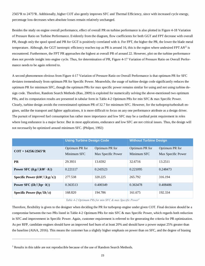
Figure 4-19 Metadata
• 𝑆𝑆𝐵𝐵𝑎𝑎%𝐸𝐸𝑖𝑖𝑖𝑖. is labeled as
Sum_of_Percent-
age_Improvement
along the vertical axis.
• COT = 1425K/2565°R
• Overall PR range is the
same as Figure 4-17.
• 𝑆𝑆𝐵𝐵𝑎𝑎%𝐸𝐸𝑖𝑖𝑖𝑖. for not using
turbine design code is
overlaid in dashed
green line on top.
8 12 16 20 24 28 32Pressure Ratio
-0,0
50
0,05
0,1
0,15
0,2
0,25
0,3
0,35
Sum
_of_
Perc
enta
ge_I
mpr
ovem
ent
0,36
0,38
0,4
0,42
0,44
0,46
0,48
0,5
0,52
Pow
er S
p. F
uel C
ons.
[lb/
(hp*
h)]
164
168
172
176
180
184
188
192
196
Spec
ific
Pow
er [h
p/(lb
/s)]
0,31
0,32
0,33
0,34
0,35
0,36
0,37
0,38
0,39
Ther
mal
Effi
cien
cy
Pressure Ratio = 10 ... 30
24
Next, the value of 𝑆𝑆𝐵𝐵𝑎𝑎%𝐸𝐸𝑖𝑖𝑖𝑖. is plotted in Figure 4-19 Sum of Percentage Improvement against Overall PR, where 𝑆𝑆𝐵𝐵𝑎𝑎%𝐸𝐸𝑖𝑖𝑖𝑖. is de-
tected to have a single peak on the interval of PR 10 to 30. Thus, Random Search Methods was again used for searching the PR for
maximum 𝑆𝑆𝐵𝐵𝑎𝑎%𝐸𝐸𝑖𝑖𝑖𝑖., whose result is demonstrated in Table 4-3 Optimum PR for maximum Sum%imp.
From the Table 4-3 Optimum PR for maximum Sum%imp, the result PR is 18.8. However, ±1 change in PR causes only around 1% of
change in corresponding Figure of Merits. Therefore, cycle PR is preliminarily chosen as 19, and may be altered within ±1 when this
number causes infinite decimal PRs for axial and centrifugal compressors when they are considered separately.
4.4. Summary of PR and COT Selections
In this section, following parameters are decided:
1. Overall PR = 19 ± 1
2. T4, namely COT = 1425𝐾𝐾/2565°𝑅𝑅
Parameters still need further studies includes: Axial & Centrifugal Compressor PR and Inlet corrected mass flow rate.
5. Constraint Analysis & Engine Sizing
To determine the inlet corrected mass flow rate of the engine, the power requirement of the aircraft need to be studied. Thus, charac-
teristics of the next generation of Single-Engine Turboprop aircraft from RFP is referred to, where aircraft performance will be trans-
lated into its power-plant specifications. In addition to the power requirement of 1600ℎ𝑝𝑝 at takeoff and 1300ℎ𝑝𝑝 at cruise (AIAA,
2016), engines are usually also sized to meet airplane performances in the following categories (Roskam, 1985, p. 89):
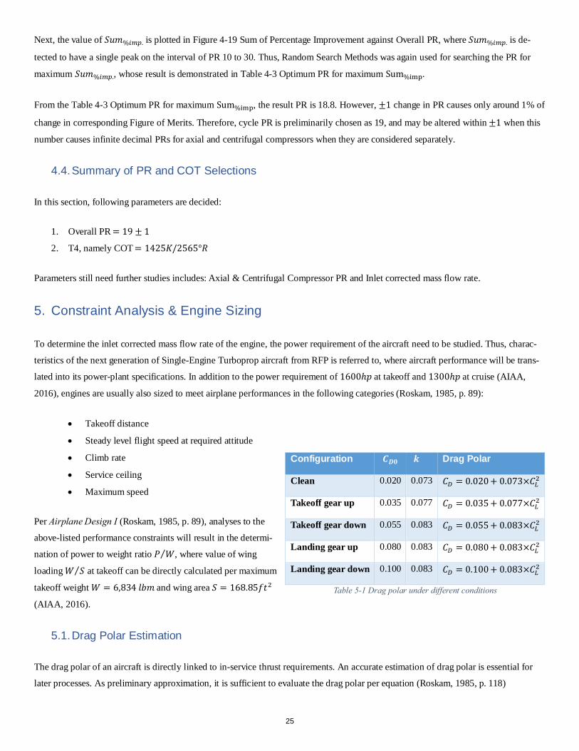
• Takeoff distance
• Steady level flight speed at required attitude
• Climb rate
• Service ceiling
• Maximum speed
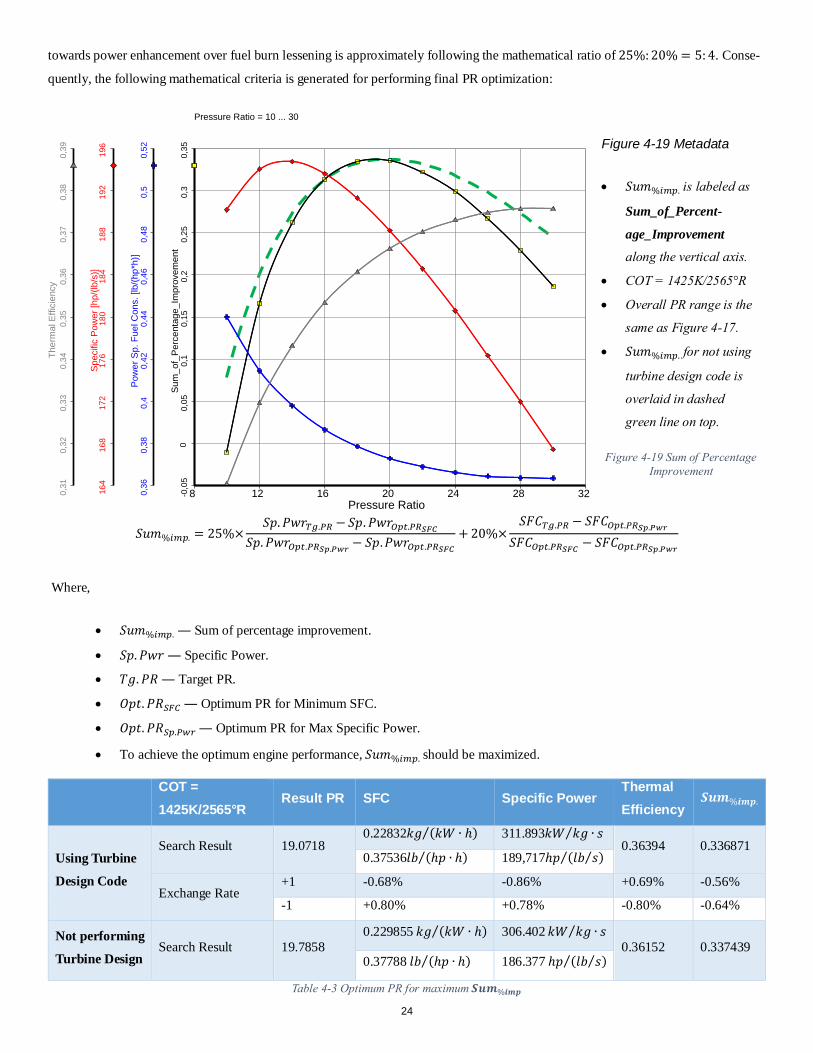
Per Airplane Design I (Roskam, 1985, p. 89), analyses to the
above-listed performance constraints will result in the determi-
nation of power to weight ratio 𝑃𝑃 𝑘𝑘⁄ , where value of wing
loading 𝑘𝑘 𝑆𝑆⁄ at takeoff can be directly calculated per maximum
takeoff weight 𝑘𝑘 = 6,834 𝑙𝑙𝑙𝑙𝑎𝑎 and wing area 𝑆𝑆 = 168.85𝑓𝑓𝑎𝑎2
(AIAA, 2016).
5.1. Drag Polar Estimation
The drag polar of an aircraft is directly linked to in-service thrust requirements. An accurate estimation of drag polar is essential for
later processes. As preliminary approximation, it is sufficient to evaluate the drag polar per equation (Roskam, 1985, p. 118)
Configuration 𝑪𝑪𝑫𝑫𝑫𝑫 𝒌𝒌 Drag Polar
Clean 0.020 0.073 𝐶𝐶𝐷𝐷 = 0.020 + 0.073×𝐶𝐶𝐿𝐿2
Takeoff gear up 0.035 0.077 𝐶𝐶𝐷𝐷 = 0.035 + 0.077×𝐶𝐶𝐿𝐿2
Takeoff gear down 0.055 0.083 𝐶𝐶𝐷𝐷 = 0.055 + 0.083×𝐶𝐶𝐿𝐿2
Landing gear up 0.080 0.083 𝐶𝐶𝐷𝐷 = 0.080 + 0.083×𝐶𝐶𝐿𝐿2
Landing gear down 0.100 0.083 𝐶𝐶𝐷𝐷 = 0.100 + 0.083×𝐶𝐶𝐿𝐿2
Table 5-1 Drag polar under different conditions
25
𝐶𝐶𝐷𝐷 = 𝐶𝐶𝐷𝐷0 + 𝑘𝑘×𝐶𝐶𝐿𝐿2
Where,
• 𝐶𝐶𝐷𝐷 ― Airplane drag polar
• 𝐶𝐶𝐷𝐷0 ― Zero-lift drag coefficient
• 𝐶𝐶𝐿𝐿 ― Lift coefficient
Using the methodologies demonstrated by Roskam (1985), the re-
sults of drag polar estimation under different conditions is pre-
sented in Table 5-1 Drag polar under different conditions.
5.2. Takeoff Constraints
Adapted from equation 3.9, Airplane Design (Roskam, 1985, p. 102), relationship between 𝑃𝑃 𝑘𝑘⁄ and 𝑘𝑘 𝑆𝑆⁄ during takeoff can be cor-
related through Formula 5-1 Takeoff Constraints.
�𝑃𝑃𝑘𝑘�
𝑇𝑇𝑂𝑂=
0.0376(𝑘𝑘 𝑆𝑆⁄ )𝑇𝑇𝑂𝑂𝜌𝜌×𝑆𝑆𝑇𝑇𝑂𝑂𝑇𝑇×𝑘𝑘 +
0.72𝐶𝐶𝐷𝐷0𝑘𝑘𝐶𝐶𝐿𝐿𝑚𝑚𝑚𝑚𝑚𝑚𝑇𝑇𝑇𝑇
+𝜇𝜇𝑇𝑇𝑘𝑘
Formula 5-1 Takeoff Constraints
Where,
• (𝑃𝑃 𝑘𝑘⁄ )𝑇𝑇𝑂𝑂 ― Takeoff power to weight ratio
• 𝑘𝑘 = 𝑙𝑙𝑖𝑖�𝜎𝜎𝑁𝑁𝐷𝐷𝑖𝑖2 𝑃𝑃𝑇𝑇𝑂𝑂⁄ �1/3, where
o For constant speed propellers, 𝑙𝑙𝑖𝑖 = 5.75 (Roskam, 1985,
p. 102)
o 𝑁𝑁 ― Number of engines; 𝐷𝐷𝑖𝑖 ― Diameter of propeller
o Term 𝑁𝑁𝐷𝐷𝑖𝑖2/𝑃𝑃𝑇𝑇𝑂𝑂 ― Propeller disk loading
o 𝜎𝜎 ― Relative density
• (𝑘𝑘 𝑆𝑆⁄ )𝑇𝑇𝑂𝑂 ― Takeoff wing loading
• 𝜌𝜌 ― Density of air
• 𝑆𝑆𝑇𝑇𝑂𝑂𝑇𝑇 ― Takeoff ground run distance
• 𝐶𝐶𝐷𝐷0 ― Zero-lift drag coefficient
• 𝜇𝜇𝑇𝑇 ― Ground friction coefficient
• 𝐶𝐶𝐿𝐿𝑚𝑚𝑚𝑚𝑚𝑚𝑇𝑇𝑇𝑇 ― Maximum takeoff lift coefficient
The results with inputs from Table 5-2 Takeoff Constraint Parameters In-
put are plotted in Figure 5-2 Takeoff Distance Constraints.
Inputs Values Comments 𝐥𝐥𝐩𝐩 5.75 (Roskam, 1985, p. 102)
𝐍𝐍 1 Single Engine
𝐍𝐍𝐃𝐃𝐩𝐩𝟐𝟐/𝐏𝐏𝐓𝐓𝐓𝐓 30hp ft2⁄ (Roskam, 1985, p. 102)
𝛔𝛔 1 ISA at SLS
𝛒𝛒 0.0765lb ft3⁄ 1.225kg m3⁄
𝐒𝐒𝐓𝐓𝐓𝐓𝐓𝐓 1600ft (Pilatus, 2002)
𝐂𝐂𝐃𝐃𝑫𝑫 0,02 Table 5-1
𝛍𝛍𝐓𝐓 0,025 (MIL-C-005011B, 1977)
𝐂𝐂𝐋𝐋𝐦𝐦𝐦𝐦𝐦𝐦𝐓𝐓𝐓𝐓 1.8 – 2.2 (Roskam, 1985, p. 107)
Table 5-2 Takeoff Constraint Parameters Input
Figure 5-1 Finding Appropriate 𝐼𝐼𝑃𝑃 (Roskam, 1985, p. 163)
0.018
0.019
0.02
0.021
0.022
0.023
0.024
0.025
10 30 50 70
Take
off p
ower
to w
eigh
t rat
io (h
p/lb
)
Takeoff Wing Loading (lb/ft^2)
Clmax=2.0 Clmax=1.8 Clmax=2.2
Figure 5-2 Takeoff Distance Constraints 26
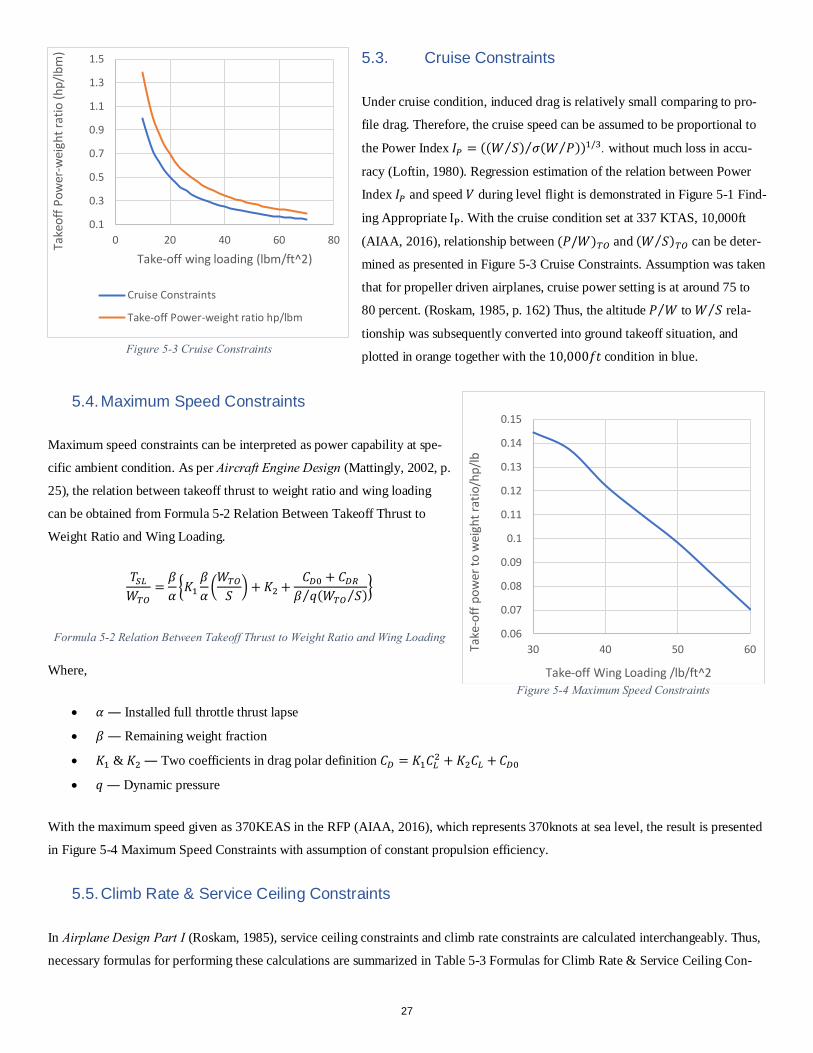
5.3. Cruise Constraints
Under cruise condition, induced drag is relatively small comparing to pro-
file drag. Therefore, the cruise speed can be assumed to be proportional to
the Power Index 𝐼𝐼𝑃𝑃 = ((𝑘𝑘 𝑆𝑆⁄ ) 𝜎𝜎(𝑘𝑘 𝑃𝑃⁄ )⁄ )1/3. without much loss in accu-
racy (Loftin, 1980). Regression estimation of the relation between Power
Index 𝐼𝐼𝑃𝑃 and speed 𝑉𝑉 during level flight is demonstrated in Figure 5-1 Find-
ing Appropriate IP. With the cruise condition set at 337 KTAS, 10,000ft
(AIAA, 2016), relationship between (𝑃𝑃/𝑘𝑘)𝑇𝑇𝑂𝑂 and (𝑘𝑘 𝑆𝑆⁄ )𝑇𝑇𝑂𝑂 can be deter-
mined as presented in Figure 5-3 Cruise Constraints. Assumption was taken
that for propeller driven airplanes, cruise power setting is at around 75 to
80 percent. (Roskam, 1985, p. 162) Thus, the altitude 𝑃𝑃 𝑘𝑘⁄ to 𝑘𝑘 𝑆𝑆⁄ rela-
tionship was subsequently converted into ground takeoff situation, and
plotted in orange together with the 10,000𝑓𝑓𝑎𝑎 condition in blue.
5.4. Maximum Speed Constraints
Maximum speed constraints can be interpreted as power capability at spe-
cific ambient condition. As per Aircraft Engine Design (Mattingly, 2002, p.
25), the relation between takeoff thrust to weight ratio and wing loading
can be obtained from Formula 5-2 Relation Between Takeoff Thrust to
Weight Ratio and Wing Loading.
𝑂𝑂𝑆𝑆𝐿𝐿𝑘𝑘𝑇𝑇𝑂𝑂
=𝛽𝛽𝛼𝛼 �𝐾𝐾1
𝛽𝛽𝛼𝛼 �
𝑘𝑘𝑇𝑇𝑂𝑂
𝑆𝑆 �+ 𝐾𝐾2 +𝐶𝐶𝐷𝐷0 + 𝐶𝐶𝐷𝐷𝑃𝑃
𝛽𝛽 𝑞𝑞(𝑘𝑘𝑇𝑇𝑂𝑂 𝑆𝑆⁄ )⁄ �
Formula 5-2 Relation Between Takeoff Thrust to Weight Ratio and Wing Loading
Where,
• 𝛼𝛼 ― Installed full throttle thrust lapse
• 𝛽𝛽 ― Remaining weight fraction
• 𝐾𝐾1 & 𝐾𝐾2 ― Two coefficients in drag polar definition 𝐶𝐶𝐷𝐷 = 𝐾𝐾1𝐶𝐶𝐿𝐿2 + 𝐾𝐾2𝐶𝐶𝐿𝐿 +𝐶𝐶𝐷𝐷0• 𝑞𝑞 ― Dynamic pressure
With the maximum speed given as 370KEAS in the RFP (AIAA, 2016), which represents 370knots at sea level, the result is presented
in Figure 5-4 Maximum Speed Constraints with assumption of constant propulsion efficiency.
5.5. Climb Rate & Service Ceiling Constraints
In Airplane Design Part I (Roskam, 1985), service ceiling constraints and climb rate constraints are calculated interchangeably. Thus,
necessary formulas for performing these calculations are summarized in Table 5-3 Formulas for Climb Rate & Service Ceiling Con-
0.1
0.3
0.5
0.7
0.9
1.1
1.3
1.5
0 20 40 60 80Take
off P
ower
-wei
ght r
atio
(hp/
lbm
)
Take-off wing loading (lbm/ft^2)
Cruise Constraints
Take-off Power-weight ratio hp/lbm
Figure 5-3 Cruise Constraints
0.06
0.07
0.08
0.09
0.1
0.11
0.12
0.13
0.14
0.15
30 40 50 60Take
-off
pow
er to
wei
ght r
atio
/hp/
lb
Take-off Wing Loading /lb/ft^2Figure 5-4 Maximum Speed Constraints
27
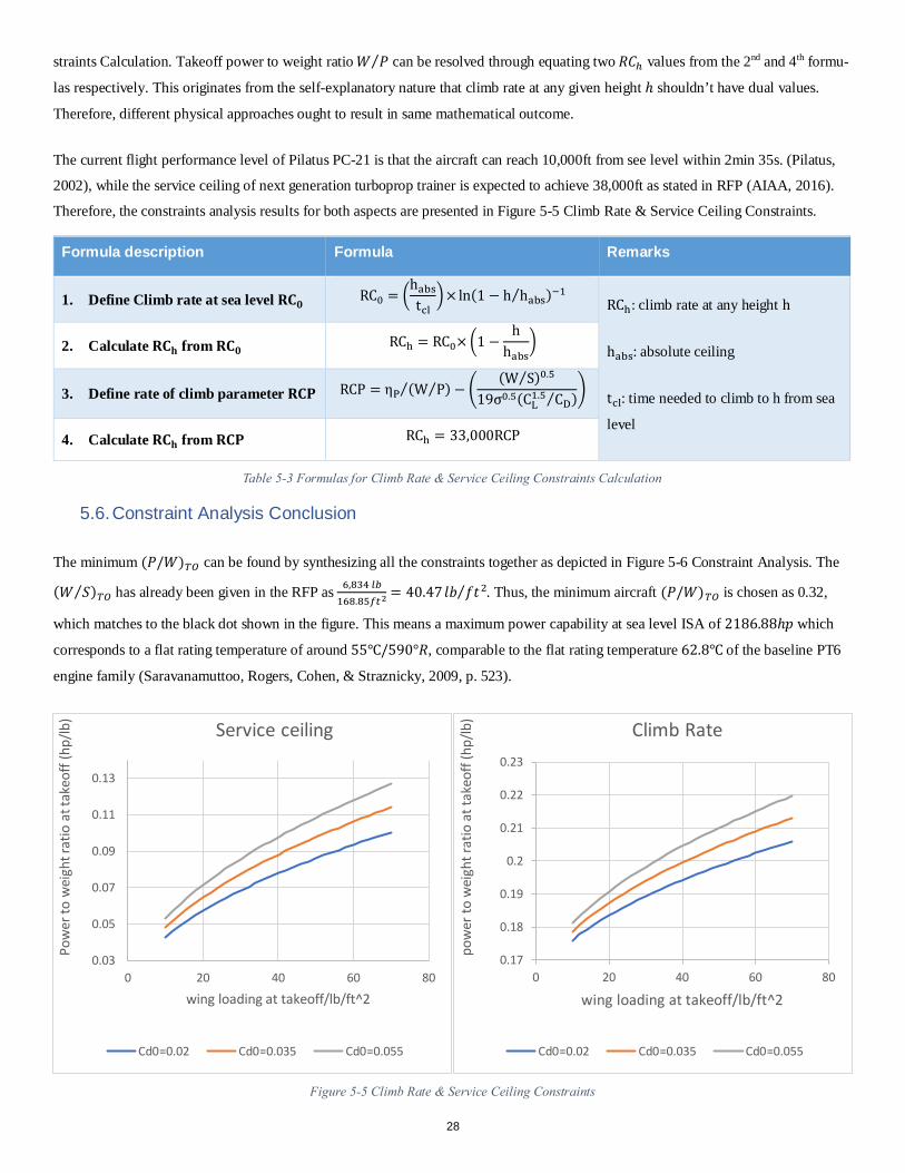
straints Calculation. Takeoff power to weight ratio 𝑘𝑘 𝑃𝑃⁄ can be resolved through equating two 𝑅𝑅𝐶𝐶ℎ values from the 2nd and 4th formu-
las respectively. This originates from the self-explanatory nature that climb rate at any given height ℎ shouldn’t have dual values.
Therefore, different physical approaches ought to result in same mathematical outcome.
The current flight performance level of Pilatus PC-21 is that the aircraft can reach 10,000ft from see level within 2min 35s. (Pilatus,
2002), while the service ceiling of next generation turboprop trainer is expected to achieve 38,000ft as stated in RFP (AIAA, 2016).
Therefore, the constraints analysis results for both aspects are presented in Figure 5-5 Climb Rate & Service Ceiling Constraints.
5.6. Constraint Analysis Conclusion
The minimum (𝑃𝑃/𝑘𝑘)𝑇𝑇𝑂𝑂 can be found by synthesizing all the constraints together as depicted in Figure 5-6 Constraint Analysis. The
(𝑘𝑘 𝑆𝑆⁄ )𝑇𝑇𝑂𝑂 has already been given in the RFP as 6,834 𝐴𝐴𝑙𝑙168.85𝑟𝑟𝐸𝐸2
= 40.47 𝑙𝑙𝑙𝑙 𝑓𝑓𝑎𝑎2⁄ . Thus, the minimum aircraft (𝑃𝑃/𝑘𝑘)𝑇𝑇𝑂𝑂 is chosen as 0.32,
which matches to the black dot shown in the figure. This means a maximum power capability at sea level ISA of 2186.88ℎ𝑝𝑝 which
corresponds to a flat rating temperature of around 55℃/590°𝑅𝑅, comparable to the flat rating temperature 62.8℃ of the baseline PT6
engine family (Saravanamuttoo, Rogers, Cohen, & Straznicky, 2009, p. 523).
Formula description Formula Remarks
1. Define Climb rate at sea level 𝐑𝐑𝐂𝐂𝑫𝑫 RC0 = �habstcl
�× ln(1 − h habs⁄ )−1 RCh: climb rate at any height h
habs: absolute ceiling
tcl: time needed to climb to h from sea
level
2. Calculate 𝐑𝐑𝐂𝐂𝐡𝐡 from 𝐑𝐑𝐂𝐂𝑫𝑫 RCh = RC0× �1 −h
habs�
3. Define rate of climb parameter 𝐑𝐑𝐂𝐂𝐏𝐏 RCP = ηP (W P⁄ )⁄ − �(W S⁄ )0.5
19σ0.5(CL1.5 CD⁄ )�
4. Calculate 𝐑𝐑𝐂𝐂𝐡𝐡 from 𝐑𝐑𝐂𝐂𝐏𝐏 RCh = 33,000RCP
Table 5-3 Formulas for Climb Rate & Service Ceiling Constraints Calculation
0.17
0.18
0.19
0.2
0.21
0.22
0.23
0 20 40 60 80
pow
er to
wei
ght r
atio
at t
akeo
ff (h
p/lb
)
wing loading at takeoff/lb/ft^2
Climb Rate
Cd0=0.02 Cd0=0.035 Cd0=0.055
0.03
0.05
0.07
0.09
0.11
0.13
0 20 40 60 80
Pow
er to
wei
ght r
atio
at t
akeo
ff (h
p/lb
)
wing loading at takeoff/lb/ft^2
Service ceiling
Cd0=0.02 Cd0=0.035 Cd0=0.055
Figure 5-5 Climb Rate & Service Ceiling Constraints
28
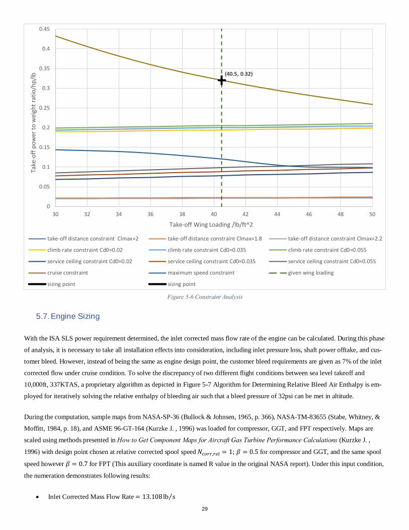
5.7. Engine Sizing
With the ISA SLS power requirement determined, the inlet corrected mass flow rate of the engine can be calculated. During this phase
of analysis, it is necessary to take all installation effects into consideration, including inlet pressure loss, shaft power offtake, and cus-
tomer bleed. However, instead of being the same as engine design point, the customer bleed requirements are given as 7% of the inlet
corrected flow under cruise condition. To solve the discrepancy of two different flight conditions between sea level takeoff and
10,000ft, 337KTAS, a proprietary algorithm as depicted in Figure 5-7 Algorithm for Determining Relative Bleed Air Enthalpy is em-
ployed for iteratively solving the relative enthalpy of bleeding air such that a bleed pressure of 32psi can be met in altitude.
During the computation, sample maps from NASA-SP-36 (Bullock & Johnsen, 1965, p. 366), NASA-TM-83655 (Stabe, Whitney, &
Moffitt, 1984, p. 18), and ASME 96-GT-164 (Kurzke J. , 1996) was loaded for compressor, GGT, and FPT respectively. Maps are
scaled using methods presented in How to Get Component Maps for Aircraft Gas Turbine Performance Calculations (Kurzke J. ,
1996) with design point chosen at relative corrected spool speed 𝑁𝑁𝑉𝑉𝑉𝑉𝐴𝐴𝐴𝐴,𝐴𝐴𝑉𝑉𝐴𝐴 = 1; 𝛽𝛽 = 0.5 for compressor and GGT, and the same spool
speed however 𝛽𝛽 = 0.7 for FPT (This auxiliary coordinate is named R value in the original NASA report). Under this input condition,
the numeration demonstrates following results:
• Inlet Corrected Mass Flow Rate = 13.108 lb s⁄
(40.5, 0.32)
0
0.05
0.1
0.15
0.2
0.25
0.3
0.35
0.4
0.45
30 32 34 36 38 40 42 44 46 48 50
Take
-off
pow
er to
wei
ght r
atio
/hp/
lb
Take-off Wing Loading /lb/ft^2
take-off distance constraint Clmax=2 take-off distance constraint Clmax=1.8 take-off distance constraint Clmax=2.2
climb rate constraint Cd0=0.02 climb rate constraint Cd0=0.035 climb rate constraint Cd0=0.055
service ceiling constraint Cd0=0.02 service ceiling constraint Cd0=0.035 service ceiling constraint Cd0=0.055
cruise constraint maximum speed constraint given wing loading
sizing point sizing point
Figure 5-6 Constraint Analysis
29
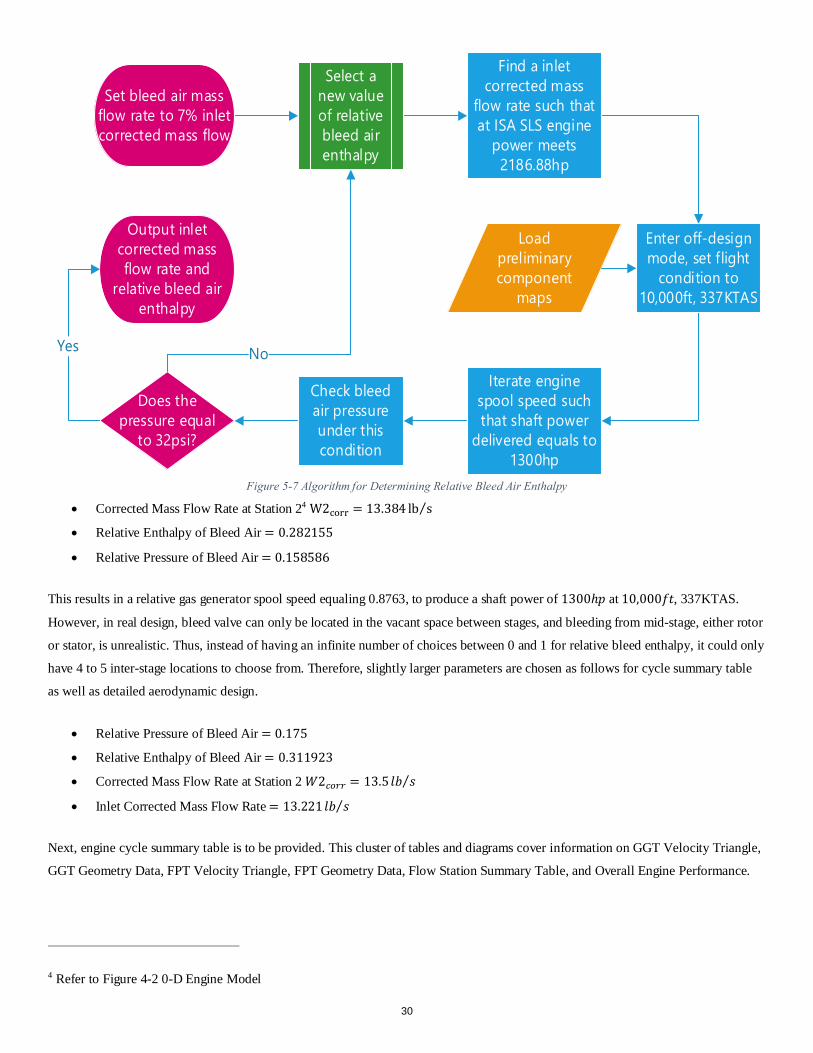
• Corrected Mass Flow Rate at Station 24 W2corr = 13.384 lb s⁄
• Relative Enthalpy of Bleed Air = 0.282155
• Relative Pressure of Bleed Air = 0.158586
This results in a relative gas generator spool speed equaling 0.8763, to produce a shaft power of 1300ℎ𝑝𝑝 at 10,000𝑓𝑓𝑎𝑎, 337KTAS.
However, in real design, bleed valve can only be located in the vacant space between stages, and bleeding from mid-stage, either rotor
or stator, is unrealistic. Thus, instead of having an infinite number of choices between 0 and 1 for relative bleed enthalpy, it could only
have 4 to 5 inter-stage locations to choose from. Therefore, slightly larger parameters are chosen as follows for cycle summary table
as well as detailed aerodynamic design.
• Relative Pressure of Bleed Air = 0.175
• Relative Enthalpy of Bleed Air = 0.311923
• Corrected Mass Flow Rate at Station 2 𝑘𝑘2𝑉𝑉𝑉𝑉𝐴𝐴𝐴𝐴 = 13.5 𝑙𝑙𝑙𝑙 𝑠𝑠⁄
• Inlet Corrected Mass Flow Rate = 13.221 𝑙𝑙𝑙𝑙 𝑠𝑠⁄
Next, engine cycle summary table is to be provided. This cluster of tables and diagrams cover information on GGT Velocity Triangle,
GGT Geometry Data, FPT Velocity Triangle, FPT Geometry Data, Flow Station Summary Table, and Overall Engine Performance.
4 Refer to Figure 4-2 0-D Engine Model
Set bleed air mass flow rate to 7% inlet corrected mass flow
Does the pressure equal
to 32psi?
Output inlet corrected mass flow rate and
relative bleed air enthalpy
Yes No
Find a inlet corrected mass
flow rate such that at ISA SLS engine
power meets 2186.88hp
Enter off-design mode, set flight
condition to 10,000ft, 337KTAS
Select a new value of relative bleed air enthalpy
Iterate engine spool speed such that shaft power
delivered equals to 1300hp
Load preliminary component
maps
Check bleed air pressure under this condition
Figure 5-7 Algorithm for Determining Relative Bleed Air Enthalpy
30
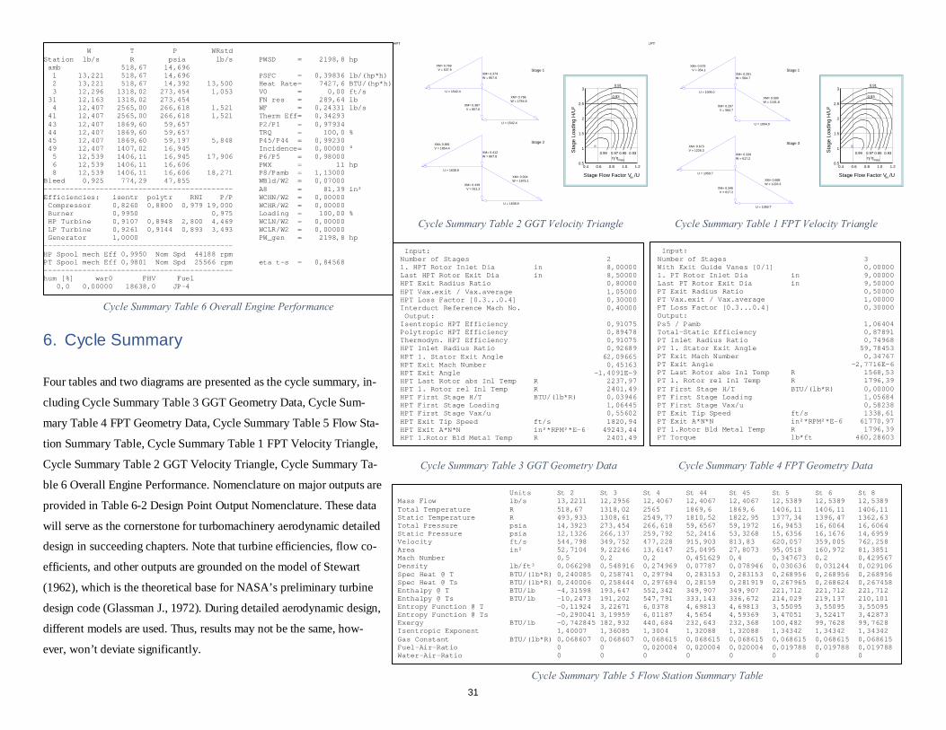
6. Cycle Summary
Four tables and two diagrams are presented as the cycle summary, in-
cluding Cycle Summary Table 3 GGT Geometry Data, Cycle Sum-
mary Table 4 FPT Geometry Data, Cycle Summary Table 5 Flow Sta-
tion Summary Table, Cycle Summary Table 1 FPT Velocity Triangle,
Cycle Summary Table 2 GGT Velocity Triangle, Cycle Summary Ta-
ble 6 Overall Engine Performance. Nomenclature on major outputs are
provided in Table 6-2 Design Point Output Nomenclature. These data
will serve as the cornerstone for turbomachinery aerodynamic detailed
design in succeeding chapters. Note that turbine efficiencies, flow co-
efficients, and other outputs are grounded on the model of Stewart
(1962), which is the theoretical base for NASA’s preliminary turbine
design code (Glassman J., 1972). During detailed aerodynamic design,
different models are used. Thus, results may not be the same, how-
ever, won’t deviate significantly.
W T P WRstd Station lb/s R psia lb/s PWSD = 2198,8 hp amb 518,67 14,696 1 13,221 518,67 14,696 PSFC = 0,39836 lb/(hp*h) 2 13,221 518,67 14,392 13,500 Heat Rate= 7427,6 BTU/(hp*h) 3 12,296 1318,02 273,454 1,053 V0 = 0,00 ft/s 31 12,163 1318,02 273,454 FN res = 289,64 lb 4 12,407 2565,00 266,618 1,521 WF = 0,24331 lb/s 41 12,407 2565,00 266,618 1,521 Therm Eff= 0,34293 43 12,407 1869,60 59,657 P2/P1 = 0,97934 44 12,407 1869,60 59,657 TRQ = 100,0 % 45 12,407 1869,60 59,197 5,848 P45/P44 = 0,99230 49 12,407 1407,02 16,945 Incidence= 0,00000 ° 5 12,539 1406,11 16,945 17,906 P6/P5 = 0,98000 6 12,539 1406,11 16,606 PWX = 11 hp 8 12,539 1406,11 16,606 18,271 P8/Pamb = 1,13000 Bleed 0,925 774,29 47,855 WBld/W2 = 0,07000 -------------------------------------------- A8 = 81,39 in² Efficiencies: isentr polytr RNI P/P WCHN/W2 = 0,00000 Compressor 0,8260 0,8800 0,979 19,000 WCHR/W2 = 0,00000 Burner 0,9950 0,975 Loading = 100,00 % HP Turbine 0,9107 0,8948 2,800 4,469 WCLN/W2 = 0,00000 LP Turbine 0,9261 0,9144 0,893 3,493 WCLR/W2 = 0,00000 Generator 1,0000 PW_gen = 2198,8 hp -------------------------------------------- HP Spool mech Eff 0,9950 Nom Spd 44188 rpm PT Spool mech Eff 0,9801 Nom Spd 25566 rpm eta t-s = 0,84568 -------------------------------------------- hum [%] war0 FHV Fuel 0,0 0,00000 18638,0 JP-4
Cycle Summary Table 6 Overall Engine Performance
Input: Number of Stages 2 1. HPT Rotor Inlet Dia in 8,00000 Last HPT Rotor Exit Dia in 8,50000 HPT Exit Radius Ratio 0,80000 HPT Vax.exit / Vax.average 1,05000 HPT Loss Factor [0.3...0.4] 0,30000 Interduct Reference Mach No. 0,40000 Output: Isentropic HPT Efficiency 0,91075 Polytropic HPT Efficiency 0,89478 Thermodyn. HPT Efficiency 0,91075 HPT Inlet Radius Ratio 0,92689 HPT 1. Stator Exit Angle 62,09665 HPT Exit Mach Number 0,45163 HPT Exit Angle -1,4091E-9HPT Last Rotor abs Inl Temp R 2237,97 HPT 1. Rotor rel Inl Temp R 2401,49 HPT First Stage H/T BTU/(lb*R) 0,03946 HPT First Stage Loading 1,06445 HPT First Stage Vax/u 0,55602 HPT Exit Tip Speed ft/s 1820,94 HPT Exit A*N*N in²*RPM²*E-6 49243,44 HPT 1.Rotor Bld Metal Temp R 2401,49
Cycle Summary Table 3 GGT Geometry Data
Input: Number of Stages 3 With Exit Guide Vanes [0/1] 0,00000 1. PT Rotor Inlet Dia in 9,00000 Last PT Rotor Exit Dia in 9,50000 PT Exit Radius Ratio 0,50000 PT Vax.exit / Vax.average 1,00000 PT Loss Factor [0.3...0.4] 0,30000 Output: Ps5 / Pamb 1,06404 Total-Static Efficiency 0,87891 PT Inlet Radius Ratio 0,74968 PT 1. Stator Exit Angle 59,78453 PT Exit Mach Number 0,34767 PT Exit Angle -2,7716E-6PT Last Rotor abs Inl Temp R 1568,53 PT 1. Rotor rel Inl Temp R 1796,39 PT First Stage H/T BTU/(lb*R) 0,00000 PT First Stage Loading 1,05684 PT First Stage Vax/u 0,58238 PT Exit Tip Speed ft/s 1338,61 PT Exit A*N*N in²*RPM²*E-6 61770,97 PT 1.Rotor Bld Metal Temp R 1796,39 PT Torque lb*ft 460,28603
Cycle Summary Table 4 FPT Geometry Data
Units St 2 St 3 St 4 St 44 St 45 St 5 St 6 St 8 Mass Flow lb/s 13,2211 12,2956 12,4067 12,4067 12,4067 12,5389 12,5389 12,5389 Total Temperature R 518,67 1318,02 2565 1869,6 1869,6 1406,11 1406,11 1406,11 Static Temperature R 493,933 1308,61 2549,77 1810,52 1822,95 1377,34 1396,47 1362,63 Total Pressure psia 14,3923 273,454 266,618 59,6567 59,1972 16,9453 16,6064 16,6064 Static Pressure psia 12,1326 266,137 259,792 52,2416 53,3268 15,6356 16,1676 14,6959 Velocity ft/s 544,798 349,752 477,228 915,903 813,83 620,057 359,005 762,258 Area in² 52,7104 9,22246 13,6147 25,0495 27,8073 95,0518 160,972 81,3851 Mach Number 0,5 0,2 0,2 0,451629 0,4 0,347673 0,2 0,429567 Density lb/ft³ 0,066298 0,548916 0,274969 0,07787 0,078946 0,030636 0,031244 0,029106 Spec Heat @ T BTU/(lb*R) 0,240085 0,258741 0,29794 0,283153 0,283153 0,268956 0,268956 0,268956 Spec Heat @ Ts BTU/(lb*R) 0,240006 0,258444 0,297694 0,28159 0,281919 0,267965 0,268624 0,267458 Enthalpy @ T BTU/lb -4,31598 193,647 552,342 349,907 349,907 221,712 221,712 221,712Enthalpy @ Ts BTU/lb -10,2473 191,202 547,791 333,143 336,672 214,029 219,137 210,101Entropy Function @ T -0,11924 3,22671 6,0378 4,69813 4,69813 3,55095 3,55095 3,55095 Entropy Function @ Ts -0,290041 3,19959 6,01187 4,5654 4,59369 3,47051 3,52417 3,42873 Exergy BTU/lb -0,742845 182,932 440,684 232,643 232,368 100,482 99,7628 99,7628Isentropic Exponent 1,40007 1,36085 1,3004 1,32088 1,32088 1,34342 1,34342 1,34342 Gas Constant BTU/(lb*R) 0,068607 0,068607 0,068615 0,068615 0,068615 0,068615 0,068615 0,068615 Fuel-Air-Ratio 0 0 0,020004 0,020004 0,020004 0,019788 0,019788 0,019788 Water-Air-Ratio 0 0 0 0 0 0 0 0
Cycle Summary Table 5 Flow Station Summary Table
Cycle Summary Table 2 GGT Velocity Triangle
0.4 0.6 0.8 1.0 1.2
3
2.5
2
1.5
1
0.5
0.99 0.97 0.95 0.93η/ηmax
Stage Flow Factor V /Uax
Stag
e Lo
adin
g H
/U²
0.91
0.93
HPT
Stage 1V = 537.9XM= 0.769
U = 1542.4
W = 857.6XM= 0.374
V = 857.6XM= 0.387
U = 1542.4
W = 1764.8XM= 0.796
Stage 2V = 1854.4XM= 0.881
U = 1638.8
W = 867.8XM= 0.412
V = 911.2XM= 0.449
U = 1638.8
W = 1875.1XM= 0.924
Cycle Summary Table 1 FPT Velocity Triangle
0.4 0.6 0.8 1.0 1.2
3
2.5
2
1.5
1
0.5
0.99 0.97 0.95 0.93η/ηmax
Stage Flow Factor V /Uax
Stag
e Lo
adin
g H
/U²
0.91
0.93
LPT
Stage 1V = 354.1XM= 0.579
U = 1004.0
W = 584.7XM= 0.291
V = 584.7XM= 0.297
U = 1004.0
W = 1161.8XM= 0.590
Stage 3
V = 1226.3XM= 0.673
U = 1059.7
W = 617.2XM= 0.339
V = 617.2XM= 0.346
U = 1059.7
W = 1226.3XM= 0.688
31
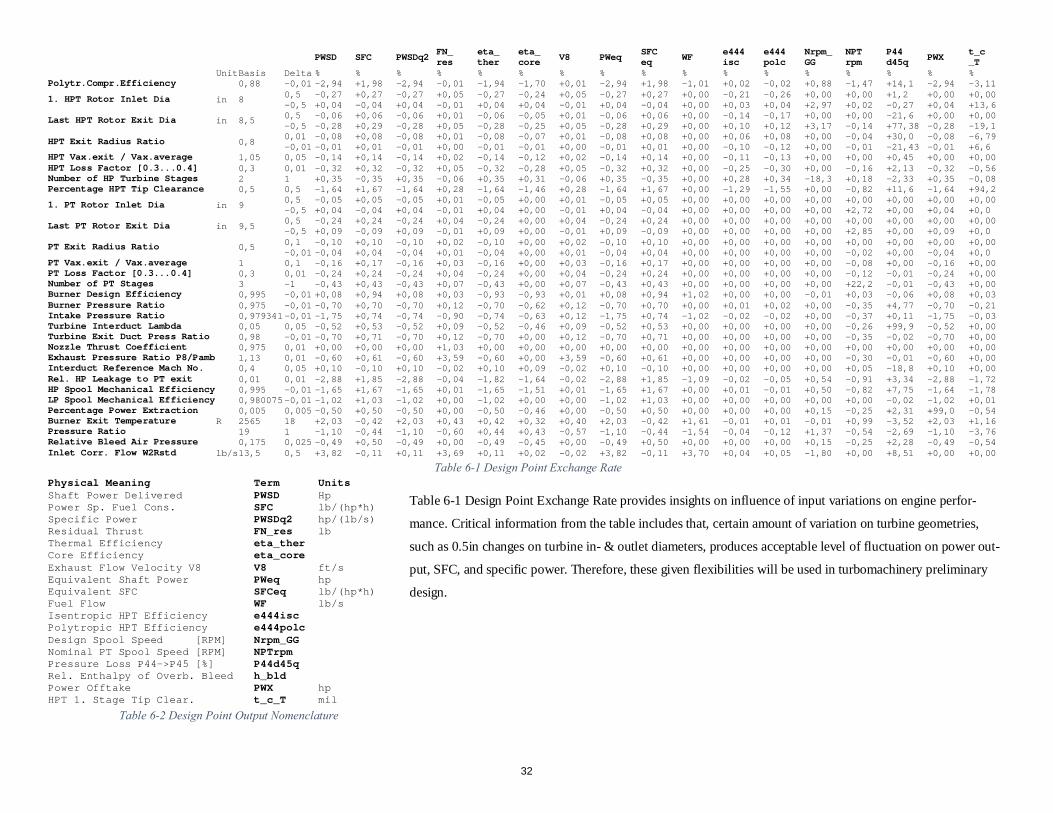
PWSD SFC PWSDq2 FN_res eta_ther
eta_ core V8 PWeq SFC
eq WF e444isc
e444polc
Nrpm_GG
NPTrpm
P44d45q PWX t_c
_T Unit Basis Delta % % % % % % % % % % % % % % % % %
Polytr.Compr.Efficiency 0,88 -0,01 -2,94 +1,98 -2,94 -0,01 -1,94 -1,70 +0,01 -2,94 +1,98 -1,01 +0,02 -0,02 +0,88 -1,47 +14,1 -2,94 -3,11
1. HPT Rotor Inlet Dia in 8 0,5 -0,27 +0,27 -0,27 +0,05 -0,27 -0,24 +0,05 -0,27 +0,27 +0,00 -0,21 -0,26 +0,00 +0,00 +1,2 +0,00 +0,00-0,5 +0,04 -0,04 +0,04 -0,01 +0,04 +0,04 -0,01 +0,04 -0,04 +0,00 +0,03 +0,04 +2,97 +0,02 -0,27 +0,04 +13,6
Last HPT Rotor Exit Dia in 8,5 0,5 -0,06 +0,06 -0,06 +0,01 -0,06 -0,05 +0,01 -0,06 +0,06 +0,00 -0,14 -0,17 +0,00 +0,00 -21,6 +0,00 +0,00-0,5 -0,28 +0,29 -0,28 +0,05 -0,28 -0,25 +0,05 -0,28 +0,29 +0,00 +0,10 +0,12 +3,17 -0,14 +77,38 -0,28 -19,1
HPT Exit Radius Ratio 0,8 0,01 -0,08 +0,08 -0,08 +0,01 -0,08 -0,07 +0,01 -0,08 +0,08 +0,00 +0,06 +0,08 +0,00 -0,04 +30,0 -0,08 -6,79-0,01 -0,01 +0,01 -0,01 +0,00 -0,01 -0,01 +0,00 -0,01 +0,01 +0,00 -0,10 -0,12 +0,00 -0,01 -21,43 -0,01 +6,6
HPT Vax.exit / Vax.average 1,05 0,05 -0,14 +0,14 -0,14 +0,02 -0,14 -0,12 +0,02 -0,14 +0,14 +0,00 -0,11 -0,13 +0,00 +0,00 +0,45 +0,00 +0,00HPT Loss Factor [0.3...0.4] 0,3 0,01 -0,32 +0,32 -0,32 +0,05 -0,32 -0,28 +0,05 -0,32 +0,32 +0,00 -0,25 -0,30 +0,00 -0,16 +2,13 -0,32 -0,56Number of HP Turbine Stages 2 1 +0,35 -0,35 +0,35 -0,06 +0,35 +0,31 -0,06 +0,35 -0,35 +0,00 +0,28 +0,34 -18,3 +0,18 -2,33 +0,35 -0,08Percentage HPT Tip Clearance 0,5 0,5 -1,64 +1,67 -1,64 +0,28 -1,64 -1,46 +0,28 -1,64 +1,67 +0,00 -1,29 -1,55 +0,00 -0,82 +11,6 -1,64 +94,2
1. PT Rotor Inlet Dia in 9 0,5 -0,05 +0,05 -0,05 +0,01 -0,05 +0,00 +0,01 -0,05 +0,05 +0,00 +0,00 +0,00 +0,00 +0,00 +0,00 +0,00 +0,00-0,5 +0,04 -0,04 +0,04 -0,01 +0,04 +0,00 -0,01 +0,04 -0,04 +0,00 +0,00 +0,00 +0,00 +2,72 +0,00 +0,04 +0,0
Last PT Rotor Exit Dia in 9,5 0,5 -0,24 +0,24 -0,24 +0,04 -0,24 +0,00 +0,04 -0,24 +0,24 +0,00 +0,00 +0,00 +0,00 +0,00 +0,00 +0,00 +0,00-0,5 +0,09 -0,09 +0,09 -0,01 +0,09 +0,00 -0,01 +0,09 -0,09 +0,00 +0,00 +0,00 +0,00 +2,85 +0,00 +0,09 +0,0
PT Exit Radius Ratio 0,5 0,1 -0,10 +0,10 -0,10 +0,02 -0,10 +0,00 +0,02 -0,10 +0,10 +0,00 +0,00 +0,00 +0,00 +0,00 +0,00 +0,00 +0,00-0,01 -0,04 +0,04 -0,04 +0,01 -0,04 +0,00 +0,01 -0,04 +0,04 +0,00 +0,00 +0,00 +0,00 -0,02 +0,00 -0,04 +0,0
PT Vax.exit / Vax.average 1 0,1 -0,16 +0,17 -0,16 +0,03 -0,16 +0,00 +0,03 -0,16 +0,17 +0,00 +0,00 +0,00 +0,00 -0,08 +0,00 -0,16 +0,00PT Loss Factor [0.3...0.4] 0,3 0,01 -0,24 +0,24 -0,24 +0,04 -0,24 +0,00 +0,04 -0,24 +0,24 +0,00 +0,00 +0,00 +0,00 -0,12 -0,01 -0,24 +0,00Number of PT Stages 3 -1 -0,43 +0,43 -0,43 +0,07 -0,43 +0,00 +0,07 -0,43 +0,43 +0,00 +0,00 +0,00 +0,00 +22,2 -0,01 -0,43 +0,00Burner Design Efficiency 0,995 -0,01 +0,08 +0,94 +0,08 +0,03 -0,93 -0,93 +0,01 +0,08 +0,94 +1,02 +0,00 +0,00 -0,01 +0,03 -0,06 +0,08 +0,03Burner Pressure Ratio 0,975 -0,01 -0,70 +0,70 -0,70 +0,12 -0,70 -0,62 +0,12 -0,70 +0,70 +0,00 +0,01 +0,02 +0,00 -0,35 +4,77 -0,70 -0,21Intake Pressure Ratio 0,979341 -0,01 -1,75 +0,74 -0,74 -0,90 -0,74 -0,63 +0,12 -1,75 +0,74 -1,02 -0,02 -0,02 +0,00 -0,37 +0,11 -1,75 -0,03Turbine Interduct Lambda 0,05 0,05 -0,52 +0,53 -0,52 +0,09 -0,52 -0,46 +0,09 -0,52 +0,53 +0,00 +0,00 +0,00 +0,00 -0,26 +99,9 -0,52 +0,00Turbine Exit Duct Press Ratio 0,98 -0,01 -0,70 +0,71 -0,70 +0,12 -0,70 +0,00 +0,12 -0,70 +0,71 +0,00 +0,00 +0,00 +0,00 -0,35 -0,02 -0,70 +0,00Nozzle Thrust Coefficient 0,975 0,01 +0,00 +0,00 +0,00 +1,03 +0,00 +0,00 +0,00 +0,00 +0,00 +0,00 +0,00 +0,00 +0,00 +0,00 +0,00 +0,00 +0,00Exhaust Pressure Ratio P8/Pamb 1,13 0,01 -0,60 +0,61 -0,60 +3,59 -0,60 +0,00 +3,59 -0,60 +0,61 +0,00 +0,00 +0,00 +0,00 -0,30 -0,01 -0,60 +0,00Interduct Reference Mach No. 0,4 0,05 +0,10 -0,10 +0,10 -0,02 +0,10 +0,09 -0,02 +0,10 -0,10 +0,00 +0,00 +0,00 +0,00 +0,05 -18,8 +0,10 +0,00Rel. HP Leakage to PT exit 0,01 0,01 -2,88 +1,85 -2,88 -0,04 -1,82 -1,64 -0,02 -2,88 +1,85 -1,09 -0,02 -0,05 +0,54 -0,91 +3,34 -2,88 -1,72HP Spool Mechanical Efficiency 0,995 -0,01 -1,65 +1,67 -1,65 +0,01 -1,65 -1,51 +0,01 -1,65 +1,67 +0,00 +0,01 -0,01 +0,50 -0,82 +7,75 -1,64 -1,78LP Spool Mechanical Efficiency 0,980075 -0,01 -1,02 +1,03 -1,02 +0,00 -1,02 +0,00 +0,00 -1,02 +1,03 +0,00 +0,00 +0,00 +0,00 +0,00 -0,02 -1,02 +0,01Percentage Power Extraction 0,005 0,005 -0,50 +0,50 -0,50 +0,00 -0,50 -0,46 +0,00 -0,50 +0,50 +0,00 +0,00 +0,00 +0,15 -0,25 +2,31 +99,0 -0,54Burner Exit Temperature R 2565 18 +2,03 -0,42 +2,03 +0,43 +0,42 +0,32 +0,40 +2,03 -0,42 +1,61 -0,01 +0,01 -0,01 +0,99 -3,52 +2,03 +1,16Pressure Ratio 19 1 -1,10 -0,44 -1,10 -0,60 +0,44 +0,43 -0,57 -1,10 -0,44 -1,54 -0,04 -0,12 +1,37 -0,54 -2,69 -1,10 -3,76Relative Bleed Air Pressure 0,175 0,025 -0,49 +0,50 -0,49 +0,00 -0,49 -0,45 +0,00 -0,49 +0,50 +0,00 +0,00 +0,00 +0,15 -0,25 +2,28 -0,49 -0,54Inlet Corr. Flow W2Rstd lb/s 13,5 0,5 +3,82 -0,11 +0,11 +3,69 +0,11 +0,02 -0,02 +3,82 -0,11 +3,70 +0,04 +0,05 -1,80 +0,00 +8,51 +0,00 +0,00
Table 6-1 Design Point Exchange Rate Physical Meaning Term Units
Table 6-1 Design Point Exchange Rate provides insights on influence of input variations on engine perfor-
mance. Critical information from the table includes that, certain amount of variation on turbine geometries,
such as 0.5in changes on turbine in- & outlet diameters, produces acceptable level of fluctuation on power out-
put, SFC, and specific power. Therefore, these given flexibilities will be used in turbomachinery preliminary
design.
Shaft Power Delivered PWSD HpPower Sp. Fuel Cons. SFC lb/(hp*h)Specific Power PWSDq2 hp/(lb/s)Residual Thrust FN_res lbThermal Efficiency eta_therCore Efficiency eta_coreExhaust Flow Velocity V8 V8 ft/sEquivalent Shaft Power PWeq hpEquivalent SFC SFCeq lb/(hp*h)Fuel Flow WF lb/sIsentropic HPT Efficiency e444iscPolytropic HPT Efficiency e444polcDesign Spool Speed [RPM] Nrpm_GGNominal PT Spool Speed [RPM] NPTrpm Pressure Loss P44->P45 [%] P44d45qRel. Enthalpy of Overb. Bleed h_bld Power Offtake PWX hpHPT 1. Stage Tip Clear. t_c_T mil
Table 6-2 Design Point Output Nomenclature
32
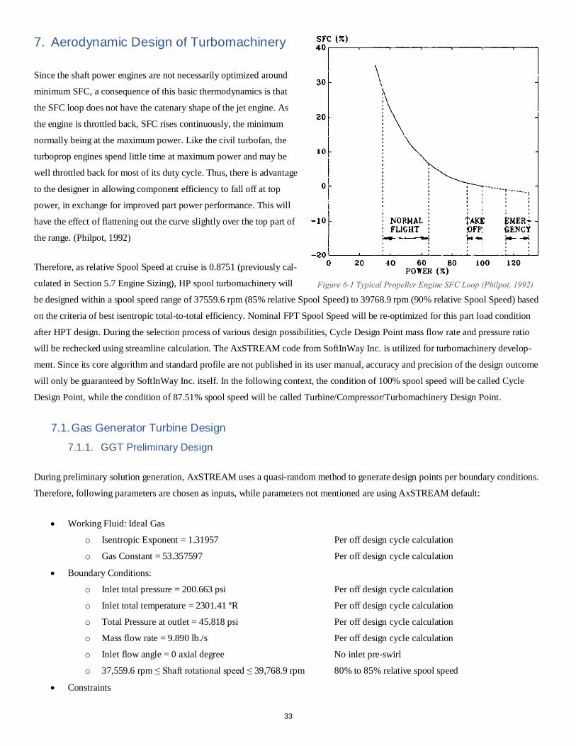
7. Aerodynamic Design of Turbomachinery
Since the shaft power engines are not necessarily optimized around
minimum SFC, a consequence of this basic thermodynamics is that
the SFC loop does not have the catenary shape of the jet engine. As
the engine is throttled back, SFC rises continuously, the minimum
normally being at the maximum power. Like the civil turbofan, the
turboprop engines spend little time at maximum power and may be
well throttled back for most of its duty cycle. Thus, there is advantage
to the designer in allowing component efficiency to fall off at top
power, in exchange for improved part power performance. This will
have the effect of flattening out the curve slightly over the top part of
the range. (Philpot, 1992)
Therefore, as relative Spool Speed at cruise is 0.8751 (previously cal-
culated in Section 5.7 Engine Sizing), HP spool turbomachinery will
be designed within a spool speed range of 37559.6 rpm (85% relative Spool Speed) to 39768.9 rpm (90% relative Spool Speed) based
on the criteria of best isentropic total-to-total efficiency. Nominal FPT Spool Speed will be re-optimized for this part load condition
after HPT design. During the selection process of various design possibilities, Cycle Design Point mass flow rate and pressure ratio
will be rechecked using streamline calculation. The AxSTREAM code from SoftInWay Inc. is utilized for turbomachinery develop-
ment. Since its core algorithm and standard profile are not published in its user manual, accuracy and precision of the design outcome
will only be guaranteed by SoftInWay Inc. itself. In the following context, the condition of 100% spool speed will be called Cycle
Design Point, while the condition of 87.51% spool speed will be called Turbine/Compressor/Turbomachinery Design Point.
7.1. Gas Generator Turbine Design 7.1.1. GGT Preliminary Design
During preliminary solution generation, AxSTREAM uses a quasi-random method to generate design points per boundary conditions.
Therefore, following parameters are chosen as inputs, while parameters not mentioned are using AxSTREAM default:
• Working Fluid: Ideal Gas
o Isentropic Exponent = 1.31957 Per off design cycle calculation
o Gas Constant = 53.357597 Per off design cycle calculation
• Boundary Conditions:
o Inlet total pressure = 200.663 psi Per off design cycle calculation
o Inlet total temperature = 2301.41 ºR Per off design cycle calculation
o Total Pressure at outlet = 45.818 psi Per off design cycle calculation
o Mass flow rate = 9.890 lb./s Per off design cycle calculation
o Inlet flow angle = 0 axial degree No inlet pre-swirl
o 37,559.6 rpm ≤ Shaft rotational speed ≤ 39,768.9 rpm 80% to 85% relative spool speed
• Constraints
Figure 6-1 Typical Propeller Engine SFC Loop (Philpot, 1992)
33
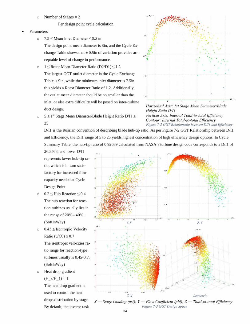
o Number of Stages = 2
Per design point cycle calculation
• Parameters
o 7.5 ≤ Mean Inlet Diameter ≤ 8.5 in
The design point mean diameter is 8in, and the Cycle Ex-
change Table shows that ± 0.5in of variation provides ac-
ceptable level of change in performance.
o 1 ≤ Rotor Mean Diameter Ratio (D2/D1) ≤ 1.2
The largest GGT outlet diameter in the Cycle Exchange
Table is 9in, while the minimum inlet diameter is 7.5in.
this yields a Rotor Diameter Ratio of 1.2. Additionally,
the outlet mean diameter should be no smaller than the
inlet, or else extra difficulty will be posed on inter-turbine
duct design.
o 5 ≤ 1st Stage Mean Diameter/Blade Height Ratio D/I1 ≤
25
D/I1 is the Russian convention of describing blade hub-tip ratio. As per Figure 7-2 GGT Relationship between D/I1
and Efficiency, the D/I1 range of 5 to 25 yields highest concentration of high efficiency design options. In Cycle
Summary Table, the hub-tip ratio of 0.92689 calculated from NASA’s turbine design code corresponds to a D/I1 of
26.3563, and lower D/I1
represents lower hub-tip ra-
tio, which is in turn satis-
factory for increased flow
capacity needed at Cycle
Design Point.
o 0.2 ≤ Hub Reaction ≤ 0.4
The hub reaction for reac-
tion turbines usually lies in
the range of 20% - 40%.
(SoftInWay)
o 0.45 ≤ Isentropic Velocity
Ratio (u/C0) ≤ 0.7
The isentropic velocities ra-
tio range for reaction-type
turbines usually is 0.45-0.7.
(SoftInWay)
o Heat drop gradient
(H_z/H_1) = 1
The heat drop gradient is
used to control the heat
drops distribution by stage.
By default, the inverse task
Horizontal Axis: 1st Stage Mean Diameter/Blade Height Ratio D/I1 Vertical Axis: Internal Total-to-total Efficiency Contour: Internal Total-to-total Efficiency Figure 7-2 GGT Relationship between D/I1 and Efficiency
Figure 7-3 GGT Design Space
Y-X Z-Y
Z-X Isometric X ― Stage Loading (psi); Y ― Flow Coefficient (phi); Z ― Total-to-total Efficiency
34
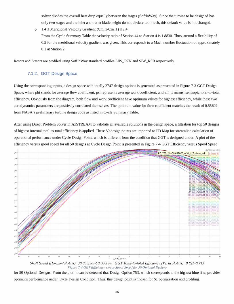
solver divides the overall heat drop equally between the stages (SoftInWay). Since the turbine to be designed has
only two stages and the inlet and outlet blade height do not deviate too much, this default value is not changed.
o 1.4 ≤ Meridional Velocity Gradient (Cm_z/Cm_1) ≤ 2.4
From the Cycle Summary Table the velocity ratio of Station 44 to Station 4 is 1.8830. Thus, around a flexibility of
0.5 for the meridional velocity gradient was given. This corresponds to a Mach number fluctuation of approximately
0.1 at Station 2.
Rotors and Stators are profiled using SoftInWay standard profiles SIW_R7N and SIW_R5B respectively.
7.1.2. GGT Design Space
Using the corresponding inputs, a design space with totally 2747 design options is generated as presented in Figure 7-3 GGT Design
Space, where phi stands for average flow coefficient, psi represents average work coefficient, and eff_tt means isentropic total-to-total
efficiency. Obviously from the diagram, both flow and work coefficient have optimum values for highest efficiency, while these two
aerodynamics parameters are positively correlated themselves. The optimum value for flow coefficient matches the result of 0.55602
from NASA’s preliminary turbine design code as listed in Cycle Summary Table.
After using Direct Problem Solver in AxSTREAM to validate all available solutions in the design space, a filtration for top 50 designs
of highest internal total-to-total efficiency is applied. These 50 design points are imported to PD Map for streamline calculation of
operational performance under Cycle Design Point, which is different from the condition that GGT is designed under. A plot of the
efficiency versus spool speed for all 50 designs at Cycle Design Point is presented in Figure 7-4 GGT Efficiency versus Spool Speed
for 50 Optional Designs. From the plot, it can be detected that Design Option 753, which corresponds to the highest blue line, provides
optimum performance under Cycle Design Condition. Thus, this design point is chosen for S1 optimization and profiling.
Shaft Speed (Horizontal Axis): 30,000rpm-50,000rpm; GGT Total-to-total Efficiency (Vertical Axis): 0.825-0.915 Figure 7-4 GGT Efficiency versus Spool Speed for 50 Optional Designs
35
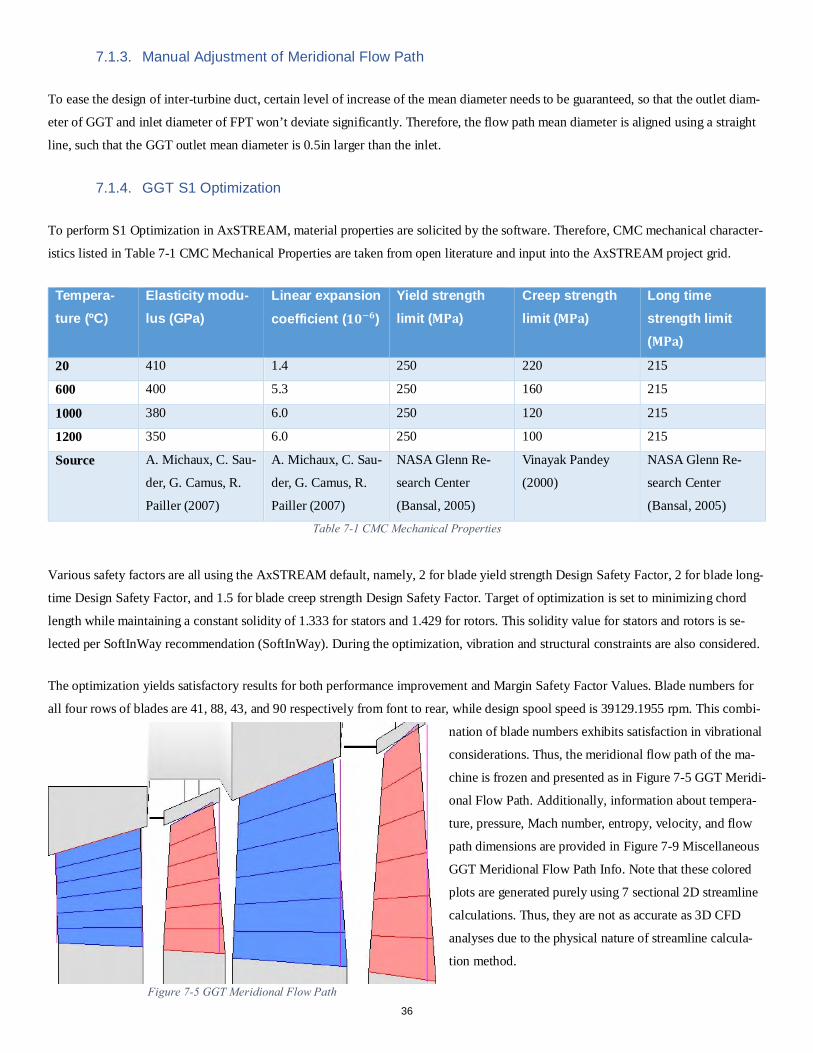
7.1.3. Manual Adjustment of Meridional Flow Path
To ease the design of inter-turbine duct, certain level of increase of the mean diameter needs to be guaranteed, so that the outlet diam-
eter of GGT and inlet diameter of FPT won’t deviate significantly. Therefore, the flow path mean diameter is aligned using a straight
line, such that the GGT outlet mean diameter is 0.5in larger than the inlet.
7.1.4. GGT S1 Optimization
To perform S1 Optimization in AxSTREAM, material properties are solicited by the software. Therefore, CMC mechanical character-
istics listed in Table 7-1 CMC Mechanical Properties are taken from open literature and input into the AxSTREAM project grid.
Tempera-ture (ºC)
Elasticity modu-lus (GPa)
Linear expansion coefficient (𝟏𝟏𝑫𝑫−𝟔𝟔)
Yield strength limit (𝐌𝐌𝐏𝐏𝐦𝐦)
Creep strength limit (𝐌𝐌𝐏𝐏𝐦𝐦)
Long time strength limit (𝐌𝐌𝐏𝐏𝐦𝐦)
20 410 1.4 250 220 215
600 400 5.3 250 160 215
1000 380 6.0 250 120 215
1200 350 6.0 250 100 215
Source A. Michaux, C. Sau-
der, G. Camus, R.
Pailler (2007)
A. Michaux, C. Sau-
der, G. Camus, R.
Pailler (2007)
NASA Glenn Re-
search Center
(Bansal, 2005)
Vinayak Pandey
(2000)
NASA Glenn Re-
search Center
(Bansal, 2005)
Table 7-1 CMC Mechanical Properties
Various safety factors are all using the AxSTREAM default, namely, 2 for blade yield strength Design Safety Factor, 2 for blade long-
time Design Safety Factor, and 1.5 for blade creep strength Design Safety Factor. Target of optimization is set to minimizing chord
length while maintaining a constant solidity of 1.333 for stators and 1.429 for rotors. This solidity value for stators and rotors is se-
lected per SoftInWay recommendation (SoftInWay). During the optimization, vibration and structural constraints are also considered.
The optimization yields satisfactory results for both performance improvement and Margin Safety Factor Values. Blade numbers for
all four rows of blades are 41, 88, 43, and 90 respectively from font to rear, while design spool speed is 39129.1955 rpm. This combi-
nation of blade numbers exhibits satisfaction in vibrational
considerations. Thus, the meridional flow path of the ma-
chine is frozen and presented as in Figure 7-5 GGT Meridi-
onal Flow Path. Additionally, information about tempera-
ture, pressure, Mach number, entropy, velocity, and flow
path dimensions are provided in Figure 7-9 Miscellaneous
GGT Meridional Flow Path Info. Note that these colored
plots are generated purely using 7 sectional 2D streamline
calculations. Thus, they are not as accurate as 3D CFD
analyses due to the physical nature of streamline calcula-
tion method.
Figure 7-5 GGT Meridional Flow Path 36
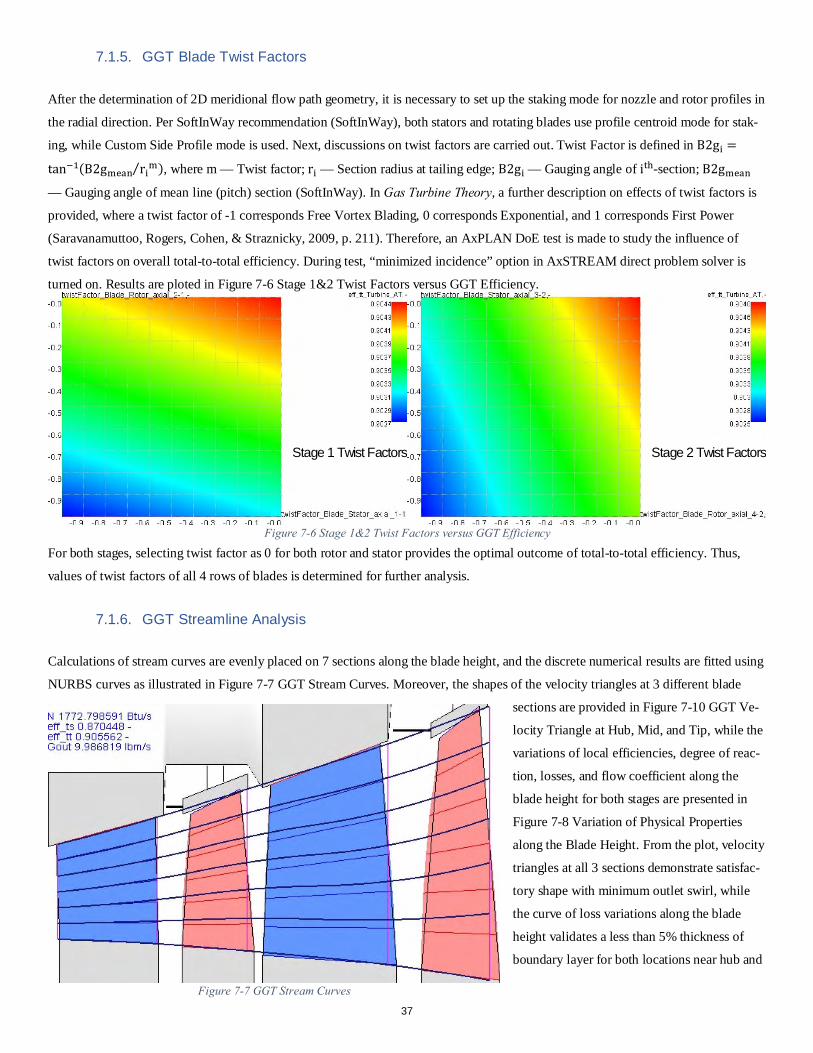
7.1.5. GGT Blade Twist Factors
After the determination of 2D meridional flow path geometry, it is necessary to set up the staking mode for nozzle and rotor profiles in
the radial direction. Per SoftInWay recommendation (SoftInWay), both stators and rotating blades use profile centroid mode for stak-
ing, while Custom Side Profile mode is used. Next, discussions on twist factors are carried out. Twist Factor is defined in B2gi =
tan−1(B2gmean rim⁄ ), where m — Twist factor; ri — Section radius at tailing edge; B2gi — Gauging angle of ith-section; B2gmean
— Gauging angle of mean line (pitch) section (SoftInWay). In Gas Turbine Theory, a further description on effects of twist factors is
provided, where a twist factor of -1 corresponds Free Vortex Blading, 0 corresponds Exponential, and 1 corresponds First Power
(Saravanamuttoo, Rogers, Cohen, & Straznicky, 2009, p. 211). Therefore, an AxPLAN DoE test is made to study the influence of
twist factors on overall total-to-total efficiency. During test, “minimized incidence” option in AxSTREAM direct problem solver is
turned on. Results are ploted in Figure 7-6 Stage 1&2 Twist Factors versus GGT Efficiency.
For both stages, selecting twist factor as 0 for both rotor and stator provides the optimal outcome of total-to-total efficiency. Thus,
values of twist factors of all 4 rows of blades is determined for further analysis.
7.1.6. GGT Streamline Analysis
Calculations of stream curves are evenly placed on 7 sections along the blade height, and the discrete numerical results are fitted using
NURBS curves as illustrated in Figure 7-7 GGT Stream Curves. Moreover, the shapes of the velocity triangles at 3 different blade
sections are provided in Figure 7-10 GGT Ve-
locity Triangle at Hub, Mid, and Tip, while the
variations of local efficiencies, degree of reac-
tion, losses, and flow coefficient along the
blade height for both stages are presented in
Figure 7-8 Variation of Physical Properties
along the Blade Height. From the plot, velocity
triangles at all 3 sections demonstrate satisfac-
tory shape with minimum outlet swirl, while
the curve of loss variations along the blade
height validates a less than 5% thickness of
boundary layer for both locations near hub and
Figure 7-6 Stage 1&2 Twist Factors versus GGT Efficiency
Stage 1 Twist Factors Stage 2 Twist Factors
Figure 7-7 GGT Stream Curves 37
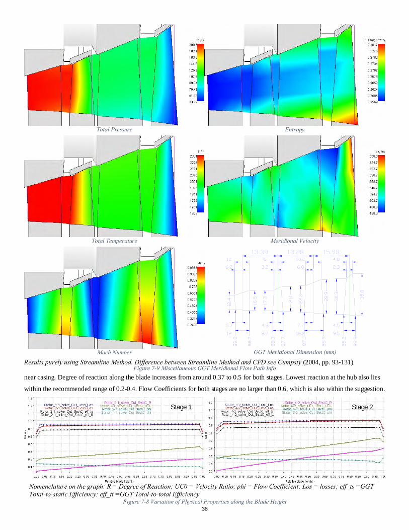
near casing. Degree of reaction along the blade increases from around 0.37 to 0.5 for both stages. Lowest reaction at the hub also lies
within the recommended range of 0.2-0.4. Flow Coefficients for both stages are no larger than 0.6, which is also within the suggestion.
Total Pressure
Total Temperature
Entropy
Meridional Velocity
Mach Number GGT Meridional Dimension (mm)
Figure 7-9 Miscellaneous GGT Meridional Flow Path Info Results purely using Streamline Method. Difference between Streamline Method and CFD see Cumpsty (2004, pp. 93-131).
Stage 1 Stage 2
Nomenclature on the graph: R = Degree of Reaction; UC0 = Velocity Ratio; phi = Flow Coefficient; Los = losses; eff_ts =GGT Total-to-static Efficiency; eff_tt =GGT Total-to-total Efficiency
Figure 7-8 Variation of Physical Properties along the Blade Height 38
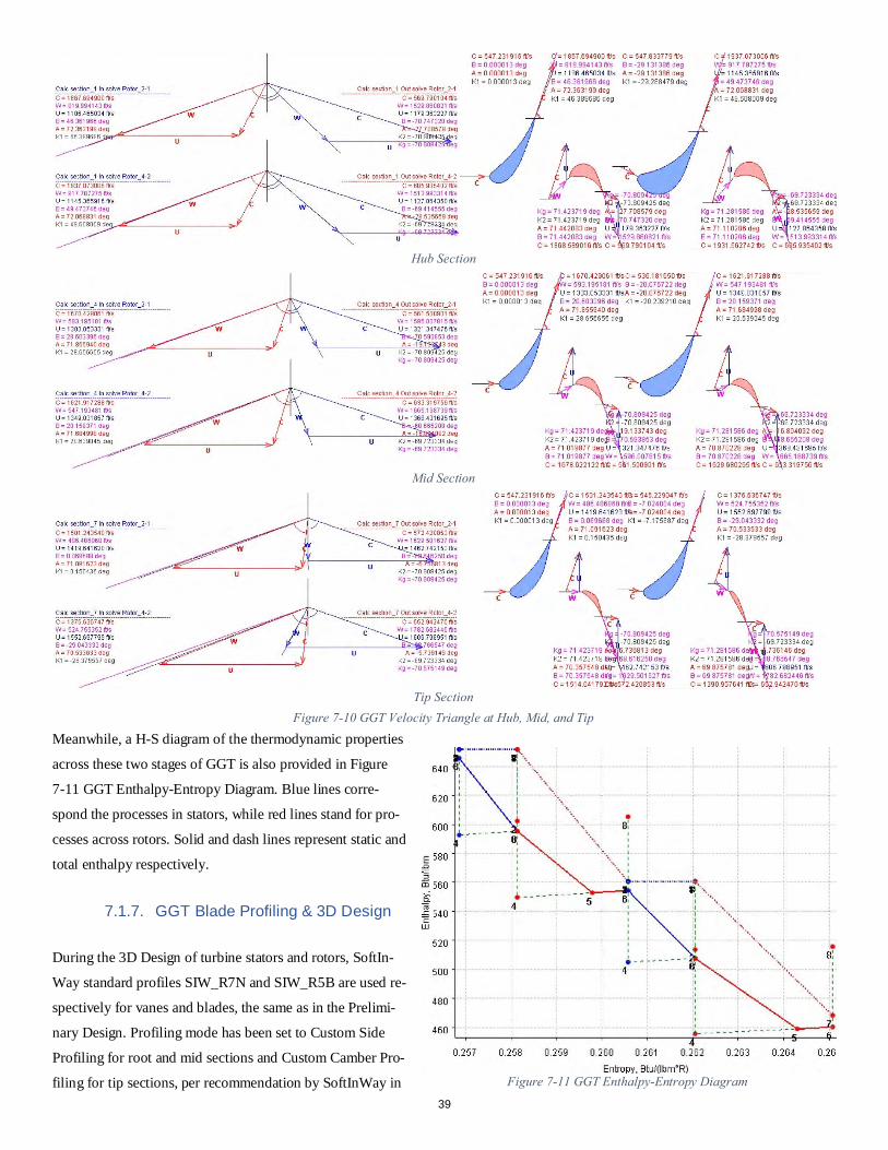
Meanwhile, a H-S diagram of the thermodynamic properties
across these two stages of GGT is also provided in Figure
7-11 GGT Enthalpy-Entropy Diagram. Blue lines corre-
spond the processes in stators, while red lines stand for pro-
cesses across rotors. Solid and dash lines represent static and
total enthalpy respectively.
7.1.7. GGT Blade Profiling & 3D Design
During the 3D Design of turbine stators and rotors, SoftIn-
Way standard profiles SIW_R7N and SIW_R5B are used re-
spectively for vanes and blades, the same as in the Prelimi-
nary Design. Profiling mode has been set to Custom Side
Profiling for root and mid sections and Custom Camber Pro-
filing for tip sections, per recommendation by SoftInWay in Figure 7-11 GGT Enthalpy-Entropy Diagram
Hub Section
Mid Section
Tip Section Figure 7-10 GGT Velocity Triangle at Hub, Mid, and Tip
39
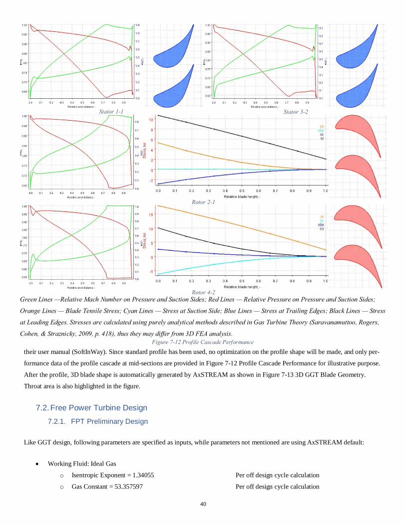
their user manual (SoftInWay). Since standard profile has been used, no optimization on the profile shape will be made, and only per-
formance data of the profile cascade at mid-sections are provided in Figure 7-12 Profile Cascade Performance for illustrative purpose.
After the profile, 3D blade shape is automatically generated by AxSTREAM as shown in Figure 7-13 3D GGT Blade Geometry.
Throat area is also highlighted in the figure.
7.2. Free Power Turbine Design 7.2.1. FPT Preliminary Design
Like GGT design, following parameters are specified as inputs, while parameters not mentioned are using AxSTREAM default:
• Working Fluid: Ideal Gas
o Isentropic Exponent = 1.34055 Per off design cycle calculation
o Gas Constant = 53.357597 Per off design cycle calculation
Figure 7-12 Profile Cascade Performance
Green Lines —Relative Mach Number on Pressure and Suction Sides; Red Lines — Relative Pressure on Pressure and Suction Sides;
Orange Lines — Blade Tensile Stress; Cyan Lines — Stress at Suction Side; Blue Lines — Stress at Trailing Edges; Black Lines — Stress
at Leading Edges. Stresses are calculated using purely analytical methods described in Gas Turbine Theory (Saravanamuttoo, Rogers,
Cohen, & Straznicky, 2009, p. 418), thus they may differ from 3D FEA analysis.
Rotor 4-2
Rotor 2-1
Stator 1-1 Stator 3-2
40
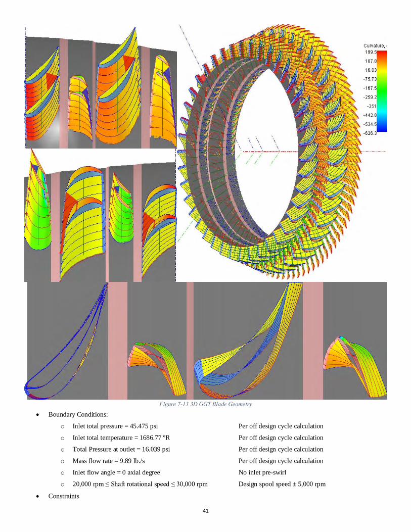
• Boundary Conditions:
o Inlet total pressure = 45.475 psi Per off design cycle calculation
o Inlet total temperature = 1686.77 ºR Per off design cycle calculation
o Total Pressure at outlet = 16.039 psi Per off design cycle calculation
o Mass flow rate = 9.89 lb./s Per off design cycle calculation
o Inlet flow angle = 0 axial degree No inlet pre-swirl
o 20,000 rpm ≤ Shaft rotational speed ≤ 30,000 rpm Design spool speed ± 5,000 rpm
• Constraints
Figure 7-13 3D GGT Blade Geometry
41
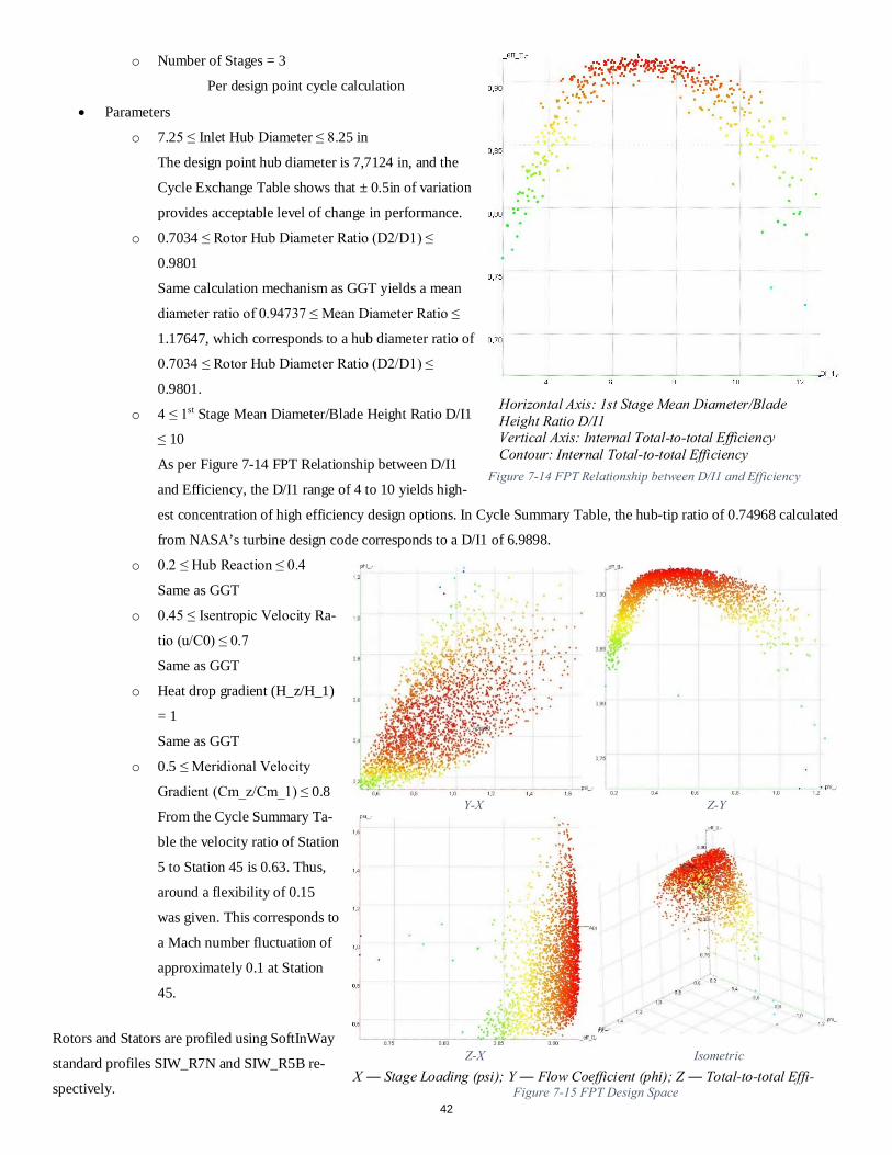
o Number of Stages = 3
Per design point cycle calculation
• Parameters
o 7.25 ≤ Inlet Hub Diameter ≤ 8.25 in
The design point hub diameter is 7,7124 in, and the
Cycle Exchange Table shows that ± 0.5in of variation
provides acceptable level of change in performance.
o 0.7034 ≤ Rotor Hub Diameter Ratio (D2/D1) ≤
0.9801
Same calculation mechanism as GGT yields a mean
diameter ratio of 0.94737 ≤ Mean Diameter Ratio ≤
1.17647, which corresponds to a hub diameter ratio of
0.7034 ≤ Rotor Hub Diameter Ratio (D2/D1) ≤
0.9801.
o 4 ≤ 1st Stage Mean Diameter/Blade Height Ratio D/I1
≤ 10
As per Figure 7-14 FPT Relationship between D/I1
and Efficiency, the D/I1 range of 4 to 10 yields high-
est concentration of high efficiency design options. In Cycle Summary Table, the hub-tip ratio of 0.74968 calculated
from NASA’s turbine design code corresponds to a D/I1 of 6.9898.
o 0.2 ≤ Hub Reaction ≤ 0.4
Same as GGT
o 0.45 ≤ Isentropic Velocity Ra-
tio (u/C0) ≤ 0.7
Same as GGT
o Heat drop gradient (H_z/H_1)
= 1
Same as GGT
o 0.5 ≤ Meridional Velocity
Gradient (Cm_z/Cm_1) ≤ 0.8
From the Cycle Summary Ta-
ble the velocity ratio of Station
5 to Station 45 is 0.63. Thus,
around a flexibility of 0.15
was given. This corresponds to
a Mach number fluctuation of
approximately 0.1 at Station
45.
Rotors and Stators are profiled using SoftInWay
standard profiles SIW_R7N and SIW_R5B re-
spectively.
Y-X Z-Y
Z-X Isometric X ― Stage Loading (psi); Y ― Flow Coefficient (phi); Z ― Total-to-total Effi-
Figure 7-15 FPT Design Space
Horizontal Axis: 1st Stage Mean Diameter/Blade Height Ratio D/I1 Vertical Axis: Internal Total-to-total Efficiency Contour: Internal Total-to-total Efficiency
Figure 7-14 FPT Relationship between D/I1 and Efficiency
42
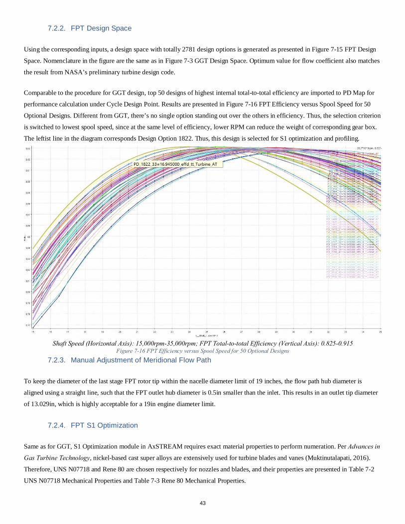
7.2.2. FPT Design Space
Using the corresponding inputs, a design space with totally 2781 design options is generated as presented in Figure 7-15 FPT Design
Space. Nomenclature in the figure are the same as in Figure 7-3 GGT Design Space. Optimum value for flow coefficient also matches
the result from NASA’s preliminary turbine design code.
Comparable to the procedure for GGT design, top 50 designs of highest internal total-to-total efficiency are imported to PD Map for
performance calculation under Cycle Design Point. Results are presented in Figure 7-16 FPT Efficiency versus Spool Speed for 50
Optional Designs. Different from GGT, there’s no single option standing out over the others in efficiency. Thus, the selection criterion
is switched to lowest spool speed, since at the same level of efficiency, lower RPM can reduce the weight of corresponding gear box.
The leftist line in the diagram corresponds Design Option 1822. Thus, this design is selected for S1 optimization and profiling.
7.2.3. Manual Adjustment of Meridional Flow Path
To keep the diameter of the last stage FPT rotor tip within the nacelle diameter limit of 19 inches, the flow path hub diameter is
aligned using a straight line, such that the FPT outlet hub diameter is 0.5in smaller than the inlet. This results in an outlet tip diameter
of 13.029in, which is highly acceptable for a 19in engine diameter limit.
7.2.4. FPT S1 Optimization
Same as for GGT, S1 Optimization module in AxSTREAM requires exact material properties to perform numeration. Per Advances in
Gas Turbine Technology, nickel-based cast super alloys are extensively used for turbine blades and vanes (Muktinutalapati, 2016).
Therefore, UNS N07718 and Rene 80 are chosen respectively for nozzles and blades, and their properties are presented in Table 7-2
UNS N07718 Mechanical Properties and Table 7-3 Rene 80 Mechanical Properties.
Shaft Speed (Horizontal Axis): 15,000rpm-35,000rpm; FPT Total-to-total Efficiency (Vertical Axis): 0.825-0.915 Figure 7-16 FPT Efficiency versus Spool Speed for 50 Optional Designs
43
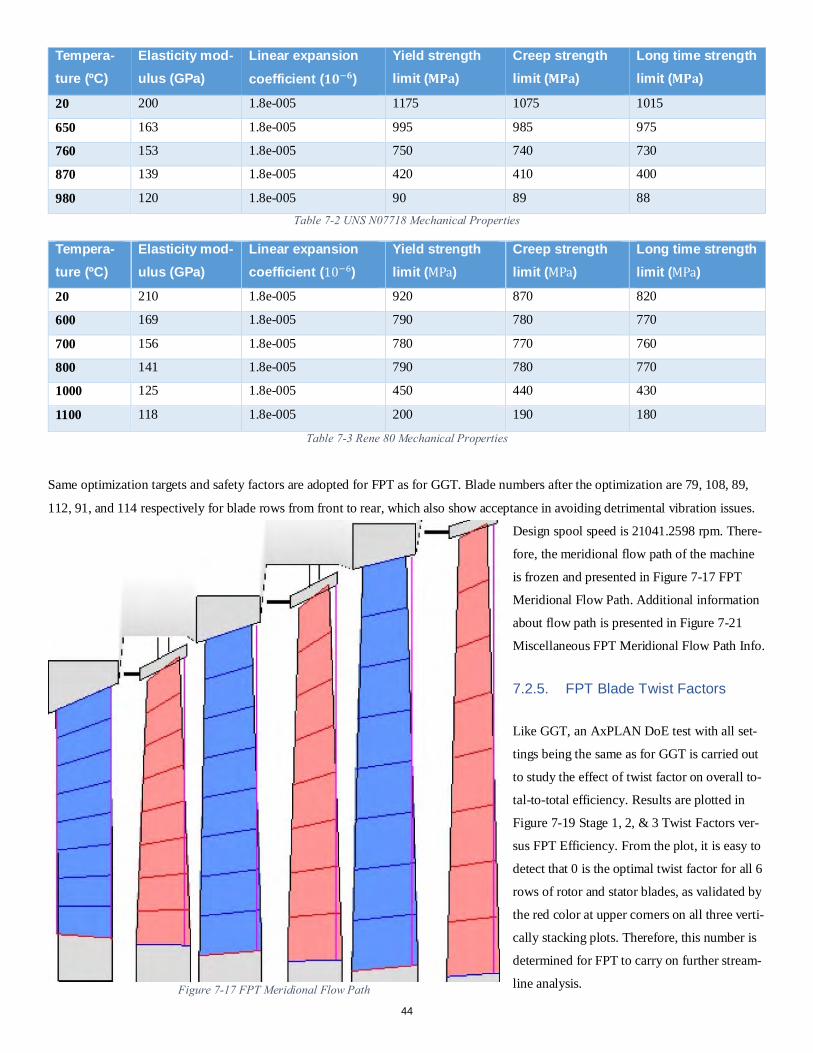
Tempera-ture (ºC)
Elasticity mod-ulus (GPa)
Linear expansion coefficient (𝟏𝟏𝑫𝑫−𝟔𝟔)
Yield strength limit (𝐌𝐌𝐏𝐏𝐦𝐦)
Creep strength limit (𝐌𝐌𝐏𝐏𝐦𝐦)
Long time strength limit (𝐌𝐌𝐏𝐏𝐦𝐦)
20 200 1.8e-005 1175 1075 1015
650 163 1.8e-005 995 985 975
760 153 1.8e-005 750 740 730
870 139 1.8e-005 420 410 400
980 120 1.8e-005 90 89 88 Table 7-2 UNS N07718 Mechanical Properties
Tempera-ture (ºC)
Elasticity mod-ulus (GPa)
Linear expansion coefficient (10−6)
Yield strength limit (MPa)
Creep strength limit (MPa)
Long time strength limit (MPa)
20 210 1.8e-005 920 870 820
600 169 1.8e-005 790 780 770
700 156 1.8e-005 780 770 760
800 141 1.8e-005 790 780 770
1000 125 1.8e-005 450 440 430
1100 118 1.8e-005 200 190 180
Table 7-3 Rene 80 Mechanical Properties
Same optimization targets and safety factors are adopted for FPT as for GGT. Blade numbers after the optimization are 79, 108, 89,
112, 91, and 114 respectively for blade rows from front to rear, which also show acceptance in avoiding detrimental vibration issues.
Design spool speed is 21041.2598 rpm. There-
fore, the meridional flow path of the machine
is frozen and presented in Figure 7-17 FPT
Meridional Flow Path. Additional information
about flow path is presented in Figure 7-21
Miscellaneous FPT Meridional Flow Path Info.
7.2.5. FPT Blade Twist Factors
Like GGT, an AxPLAN DoE test with all set-
tings being the same as for GGT is carried out
to study the effect of twist factor on overall to-
tal-to-total efficiency. Results are plotted in
Figure 7-19 Stage 1, 2, & 3 Twist Factors ver-
sus FPT Efficiency. From the plot, it is easy to
detect that 0 is the optimal twist factor for all 6
rows of rotor and stator blades, as validated by
the red color at upper corners on all three verti-
cally stacking plots. Therefore, this number is
determined for FPT to carry on further stream-
line analysis. Figure 7-17 FPT Meridional Flow Path 44
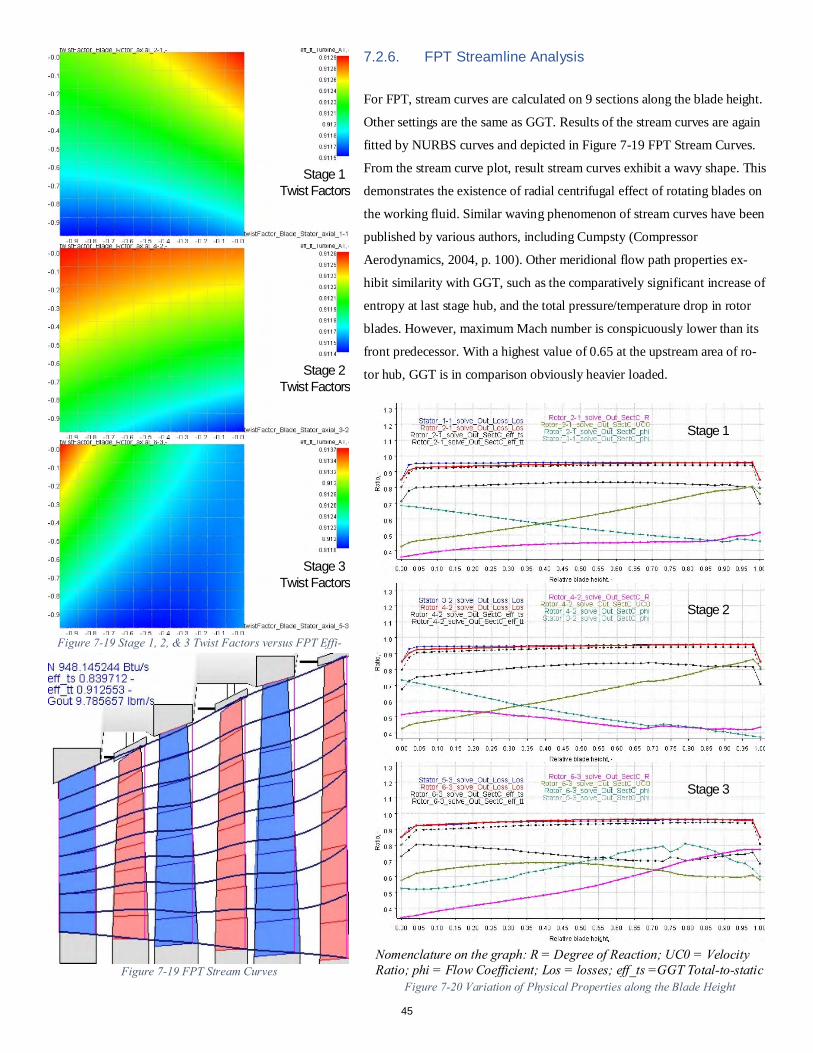
7.2.6. FPT Streamline Analysis
For FPT, stream curves are calculated on 9 sections along the blade height.
Other settings are the same as GGT. Results of the stream curves are again
fitted by NURBS curves and depicted in Figure 7-19 FPT Stream Curves.
From the stream curve plot, result stream curves exhibit a wavy shape. This
demonstrates the existence of radial centrifugal effect of rotating blades on
the working fluid. Similar waving phenomenon of stream curves have been
published by various authors, including Cumpsty (Compressor
Aerodynamics, 2004, p. 100). Other meridional flow path properties ex-
hibit similarity with GGT, such as the comparatively significant increase of
entropy at last stage hub, and the total pressure/temperature drop in rotor
blades. However, maximum Mach number is conspicuously lower than its
front predecessor. With a highest value of 0.65 at the upstream area of ro-
tor hub, GGT is in comparison obviously heavier loaded.
Stage 1 Twist Factors
Stage 2 Twist Factors
Stage 3 Twist Factors
Figure 7-19 Stage 1, 2, & 3 Twist Factors versus FPT Effi-i
Figure 7-19 FPT Stream Curves
Stage 1
Stage 2
Stage 3
Nomenclature on the graph: R = Degree of Reaction; UC0 = Velocity Ratio; phi = Flow Coefficient; Los = losses; eff_ts =GGT Total-to-static Efficiency; eff_tt =GGT Total-to-total Efficiency Figure 7-20 Variation of Physical Properties along the Blade Height
45
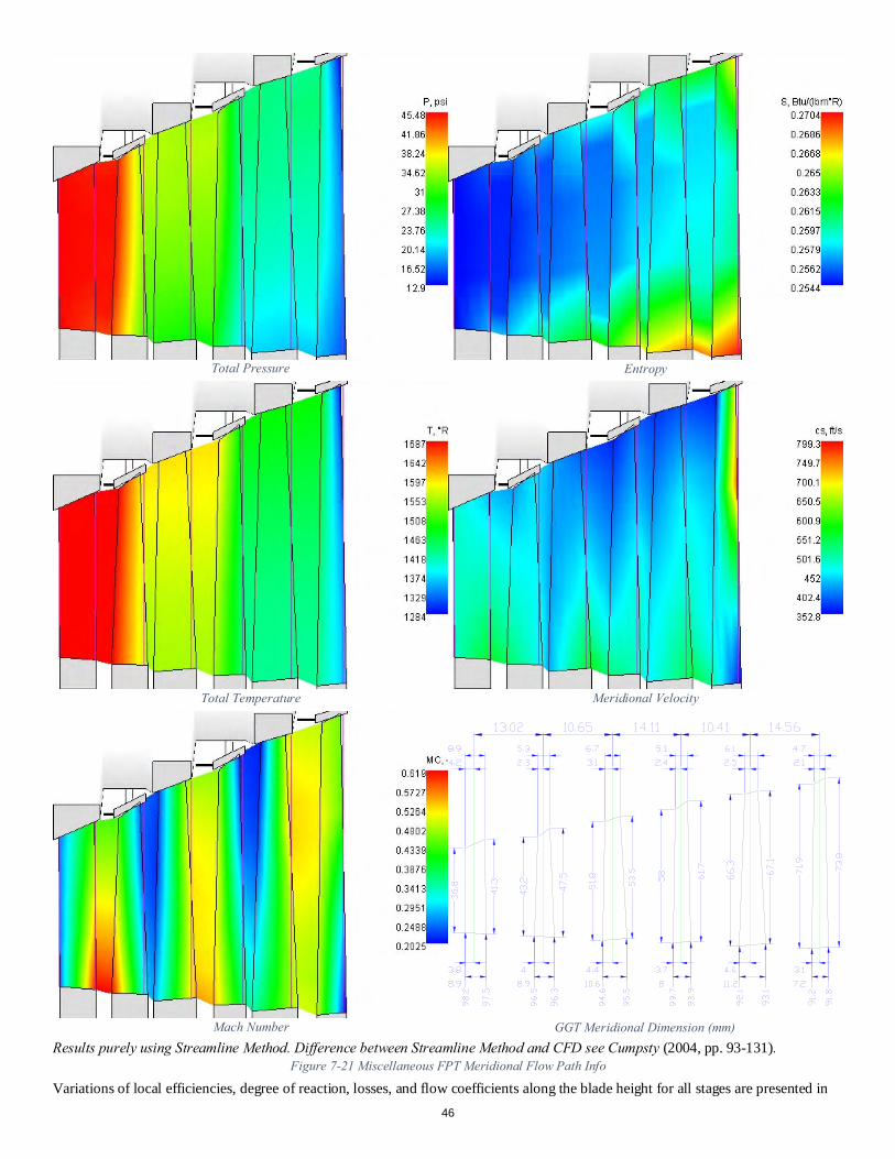
Variations of local efficiencies, degree of reaction, losses, and flow coefficients along the blade height for all stages are presented in
Total Pressure
Total Temperature
Entropy
Meridional Velocity
Mach Number Results purely using Streamline Method. Difference between Streamline Method and CFD see Cumpsty (2004, pp. 93-131).
Figure 7-21 Miscellaneous FPT Meridional Flow Path Info
GGT Meridional Dimension (mm)
46
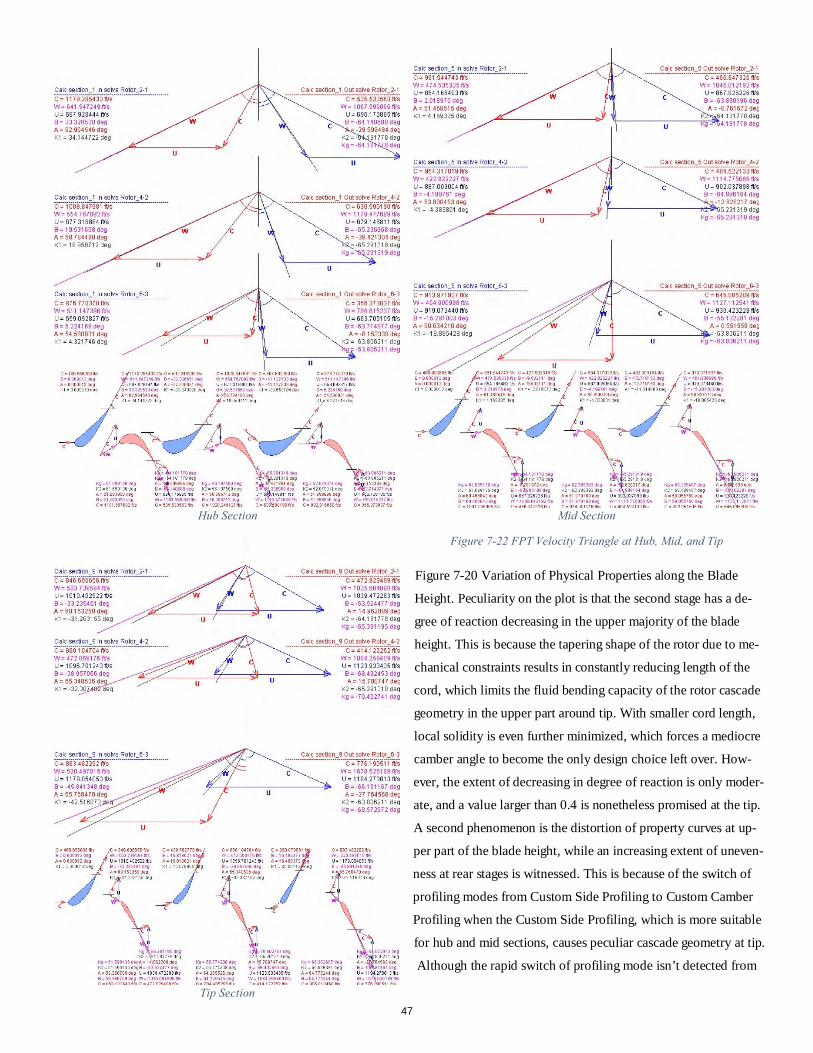
Figure 7-20 Variation of Physical Properties along the Blade
Height. Peculiarity on the plot is that the second stage has a de-
gree of reaction decreasing in the upper majority of the blade
height. This is because the tapering shape of the rotor due to me-
chanical constraints results in constantly reducing length of the
cord, which limits the fluid bending capacity of the rotor cascade
geometry in the upper part around tip. With smaller cord length,
local solidity is even further minimized, which forces a mediocre
camber angle to become the only design choice left over. How-
ever, the extent of decreasing in degree of reaction is only moder-
ate, and a value larger than 0.4 is nonetheless promised at the tip.
A second phenomenon is the distortion of property curves at up-
per part of the blade height, while an increasing extent of uneven-
ness at rear stages is witnessed. This is because of the switch of
profiling modes from Custom Side Profiling to Custom Camber
Profiling when the Custom Side Profiling, which is more suitable
for hub and mid sections, causes peculiar cascade geometry at tip.
Although the rapid switch of profiling mode isn’t detected from
Tip Section
Hub Section Mid Section
Figure 7-22 FPT Velocity Triangle at Hub, Mid, and Tip
47
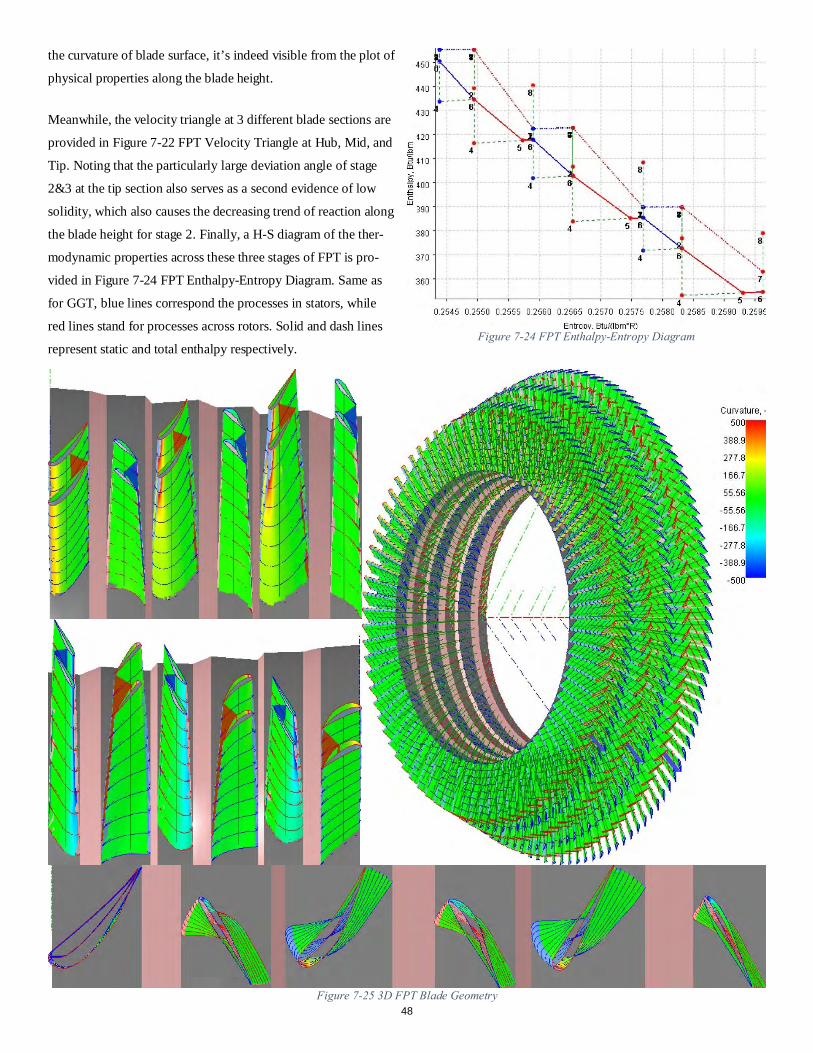
the curvature of blade surface, it’s indeed visible from the plot of
physical properties along the blade height.
Meanwhile, the velocity triangle at 3 different blade sections are
provided in Figure 7-22 FPT Velocity Triangle at Hub, Mid, and
Tip. Noting that the particularly large deviation angle of stage
2&3 at the tip section also serves as a second evidence of low
solidity, which also causes the decreasing trend of reaction along
the blade height for stage 2. Finally, a H-S diagram of the ther-
modynamic properties across these three stages of FPT is pro-
vided in Figure 7-24 FPT Enthalpy-Entropy Diagram. Same as
for GGT, blue lines correspond the processes in stators, while
red lines stand for processes across rotors. Solid and dash lines
represent static and total enthalpy respectively.
Figure 7-23 FPT Enthalpy-Entropy Diagram Figure 7-24 FPT Enthalpy-Entropy Diagram
48Figure 7-25 3D FPT Blade Geometry
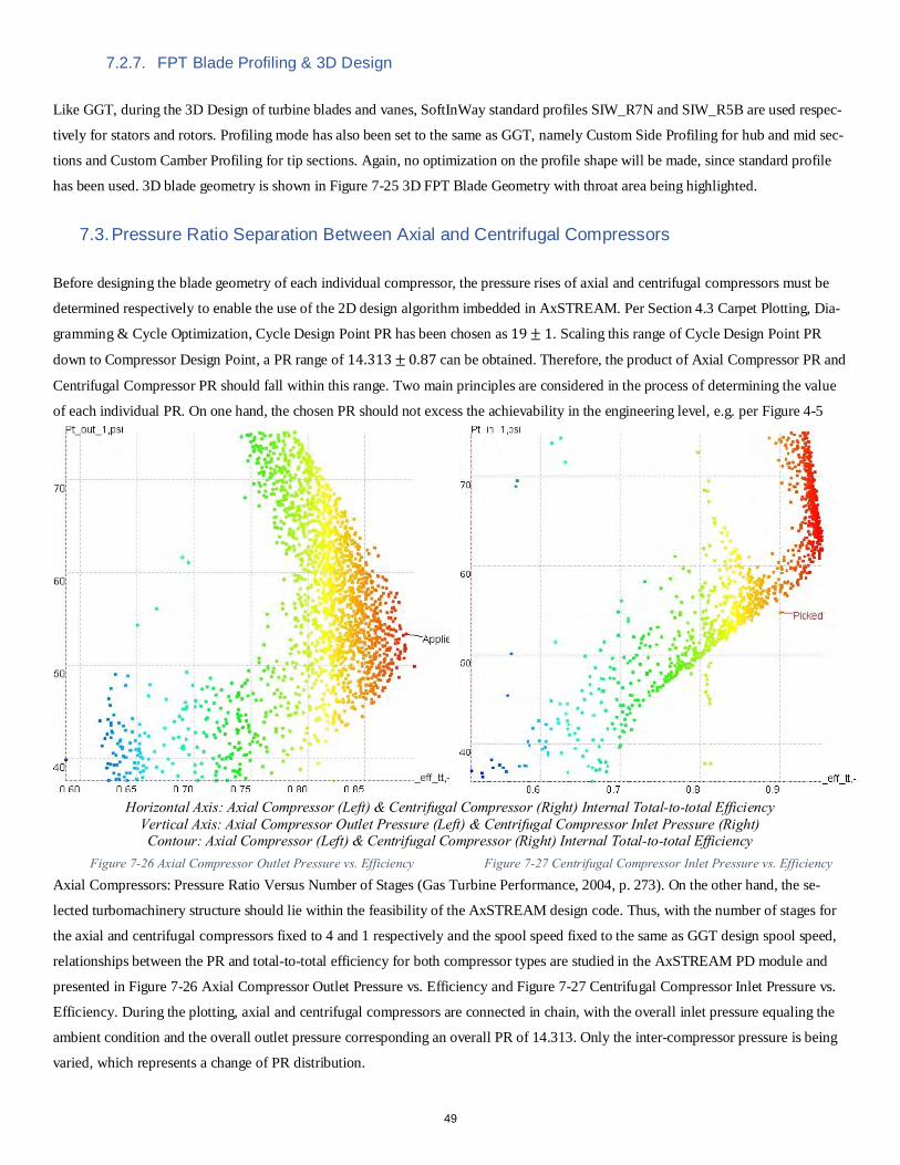
7.2.7. FPT Blade Profiling & 3D Design
Like GGT, during the 3D Design of turbine blades and vanes, SoftInWay standard profiles SIW_R7N and SIW_R5B are used respec-
tively for stators and rotors. Profiling mode has also been set to the same as GGT, namely Custom Side Profiling for hub and mid sec-
tions and Custom Camber Profiling for tip sections. Again, no optimization on the profile shape will be made, since standard profile
has been used. 3D blade geometry is shown in Figure 7-25 3D FPT Blade Geometry with throat area being highlighted.
7.3. Pressure Ratio Separation Between Axial and Centrifugal Compressors
Before designing the blade geometry of each individual compressor, the pressure rises of axial and centrifugal compressors must be
determined respectively to enable the use of the 2D design algorithm imbedded in AxSTREAM. Per Section 4.3 Carpet Plotting, Dia-
gramming & Cycle Optimization, Cycle Design Point PR has been chosen as 19 ± 1. Scaling this range of Cycle Design Point PR
down to Compressor Design Point, a PR range of 14.313 ± 0.87 can be obtained. Therefore, the product of Axial Compressor PR and
Centrifugal Compressor PR should fall within this range. Two main principles are considered in the process of determining the value
of each individual PR. On one hand, the chosen PR should not excess the achievability in the engineering level, e.g. per Figure 4-5
Axial Compressors: Pressure Ratio Versus Number of Stages (Gas Turbine Performance, 2004, p. 273). On the other hand, the se-
lected turbomachinery structure should lie within the feasibility of the AxSTREAM design code. Thus, with the number of stages for
the axial and centrifugal compressors fixed to 4 and 1 respectively and the spool speed fixed to the same as GGT design spool speed,
relationships between the PR and total-to-total efficiency for both compressor types are studied in the AxSTREAM PD module and
presented in Figure 7-26 Axial Compressor Outlet Pressure vs. Efficiency and Figure 7-27 Centrifugal Compressor Inlet Pressure vs.
Efficiency. During the plotting, axial and centrifugal compressors are connected in chain, with the overall inlet pressure equaling the
ambient condition and the overall outlet pressure corresponding an overall PR of 14.313. Only the inter-compressor pressure is being
varied, which represents a change of PR distribution.
Figure 7-26 Axial Compressor Outlet Pressure vs. Efficiency Figure 7-27 Centrifugal Compressor Inlet Pressure vs. Efficiency
Horizontal Axis: Axial Compressor (Left) & Centrifugal Compressor (Right) Internal Total-to-total Efficiency Vertical Axis: Axial Compressor Outlet Pressure (Left) & Centrifugal Compressor Inlet Pressure (Right) Contour: Axial Compressor (Left) & Centrifugal Compressor (Right) Internal Total-to-total Efficiency
49
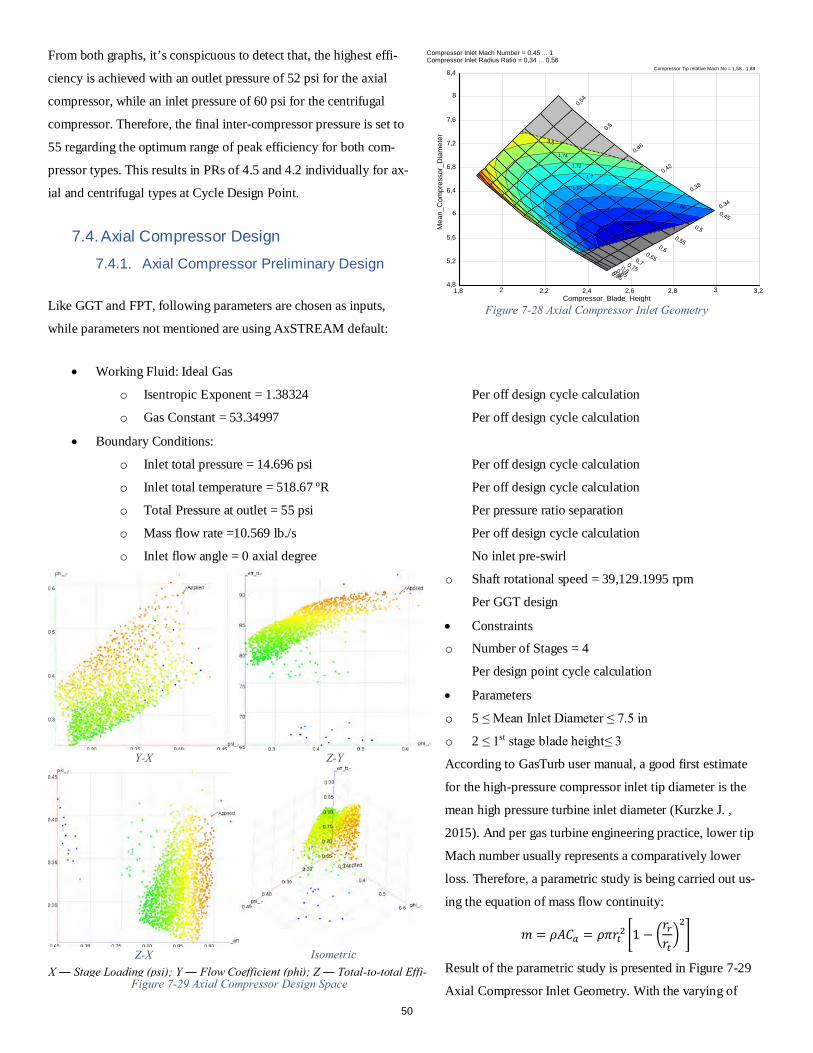
From both graphs, it’s conspicuous to detect that, the highest effi-
ciency is achieved with an outlet pressure of 52 psi for the axial
compressor, while an inlet pressure of 60 psi for the centrifugal
compressor. Therefore, the final inter-compressor pressure is set to
55 regarding the optimum range of peak efficiency for both com-
pressor types. This results in PRs of 4.5 and 4.2 individually for ax-
ial and centrifugal types at Cycle Design Point.
7.4. Axial Compressor Design 7.4.1. Axial Compressor Preliminary Design
Like GGT and FPT, following parameters are chosen as inputs,
while parameters not mentioned are using AxSTREAM default:
• Working Fluid: Ideal Gas
o Isentropic Exponent = 1.38324 Per off design cycle calculation
o Gas Constant = 53.34997 Per off design cycle calculation
• Boundary Conditions:
o Inlet total pressure = 14.696 psi Per off design cycle calculation
o Inlet total temperature = 518.67 ºR Per off design cycle calculation
o Total Pressure at outlet = 55 psi Per pressure ratio separation
o Mass flow rate =10.569 lb./s Per off design cycle calculation
o Inlet flow angle = 0 axial degree No inlet pre-swirl
o Shaft rotational speed = 39,129.1995 rpm
Per GGT design
• Constraints
o Number of Stages = 4
Per design point cycle calculation
• Parameters
o 5 ≤ Mean Inlet Diameter ≤ 7.5 in
o 2 ≤ 1st stage blade height≤ 3
According to GasTurb user manual, a good first estimate
for the high-pressure compressor inlet tip diameter is the
mean high pressure turbine inlet diameter (Kurzke J. ,
2015). And per gas turbine engineering practice, lower tip
Mach number usually represents a comparatively lower
loss. Therefore, a parametric study is being carried out us-
ing the equation of mass flow continuity:
𝑎𝑎 = 𝜌𝜌𝐴𝐴𝐶𝐶𝐴𝐴 = 𝜌𝜌𝜌𝜌𝑟𝑟𝐸𝐸2 �1 − �𝑟𝑟𝐴𝐴𝑟𝑟𝐸𝐸�2�
Result of the parametric study is presented in Figure 7-29
Axial Compressor Inlet Geometry. With the varying of
Y-X Z-Y
Z-X IsometricX ― Stage Loading (psi); Y ― Flow Coefficient (phi); Z ― Total-to-total Effi-
Figure 7-29 Axial Compressor Design Space
1,8 2 2,2 2,4 2,6 2,8 3 3,2Compressor_Blade_Height
4,8
5,2
5,6
6
6,4
6,8
7,2
7,6
8
8,4
Mea
n_C
ompr
esso
r_D
iam
eter
Compressor Inlet Mach Number = 0,45 ... 1 Compressor Inlet Radius Ratio = 0,34 ... 0,56
Compressor Tip relative Mach No = 1,58...1,88
1,6
1,62
1,641,66
1,68
1,7
1,72
1,741,76
1,78
1,8
1,82
1,84
1,86
9,5
3
0,34
0,38
0,42
0,46
0,5
0,54
0,450,5
0,550,6
0,650,70,750,80,850,90,95
Figure 7-28 Axial Compressor Inlet Geometry
50
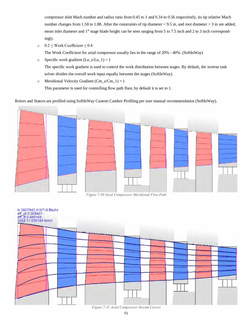
compressor inlet Mach number and radius ratio from 0.45 to 1 and 0.34 to 0.56 respectively, its tip relative Mach
number changes from 1.58 to 1.88. After the constraints of tip diameter < 9.5 in, and root diameter > 3 in are added,
mean inlet diameter and 1st stage blade height can be seen ranging from 5 to 7.5 inch and 2 to 3 inch correspond-
ingly.
o 0.2 ≤ Work Coefficient ≤ 0.4
The Work Coefficient for axial compressor usually lies in the range of 20% - 40%. (SoftInWay)
o Specific work gradient (Lu_z/Lu_1) = 1
The specific work gradient is used to control the work distribution between stages. By default, the inverse task
solver divides the overall work input equally between the stages (SoftInWay).
o Meridional Velocity Gradient (Cm_z/Cm_1) = 1
This parameter is used for controlling flow path flare, by default it is set to 1.
Rotors and Stators are profiled using SoftInWay Custom Camber Profiling per user manual recommendation (SoftInWay).
Figure 7-30 Axial Compressor Meridional Flow Path
Figure 7-31 Axial Compressor Stream Curves 51
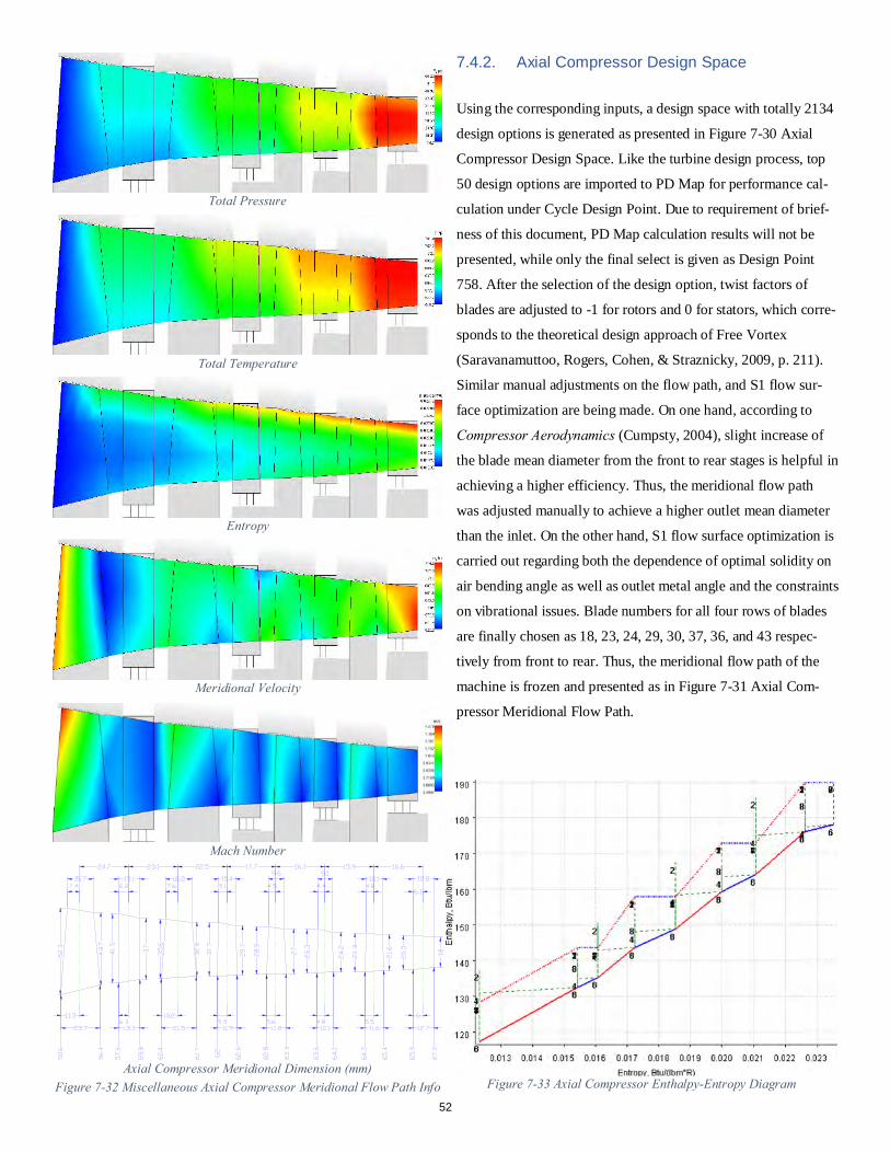
7.4.2. Axial Compressor Design Space
Using the corresponding inputs, a design space with totally 2134
design options is generated as presented in Figure 7-30 Axial
Compressor Design Space. Like the turbine design process, top
50 design options are imported to PD Map for performance cal-
culation under Cycle Design Point. Due to requirement of brief-
ness of this document, PD Map calculation results will not be
presented, while only the final select is given as Design Point
758. After the selection of the design option, twist factors of
blades are adjusted to -1 for rotors and 0 for stators, which corre-
sponds to the theoretical design approach of Free Vortex
(Saravanamuttoo, Rogers, Cohen, & Straznicky, 2009, p. 211).
Similar manual adjustments on the flow path, and S1 flow sur-
face optimization are being made. On one hand, according to
Compressor Aerodynamics (Cumpsty, 2004), slight increase of
the blade mean diameter from the front to rear stages is helpful in
achieving a higher efficiency. Thus, the meridional flow path
was adjusted manually to achieve a higher outlet mean diameter
than the inlet. On the other hand, S1 flow surface optimization is
carried out regarding both the dependence of optimal solidity on
air bending angle as well as outlet metal angle and the constraints
on vibrational issues. Blade numbers for all four rows of blades
are finally chosen as 18, 23, 24, 29, 30, 37, 36, and 43 respec-
tively from front to rear. Thus, the meridional flow path of the
machine is frozen and presented as in Figure 7-31 Axial Com-
pressor Meridional Flow Path.
Figure 7-33 Axial Compressor Enthalpy-Entropy Diagram
Total Pressure
Mach Number
Meridional Velocity
Entropy
Total Temperature
Figure 7-32 Miscellaneous Axial Compressor Meridional Flow Path Info Axial Compressor Meridional Dimension (mm)
52
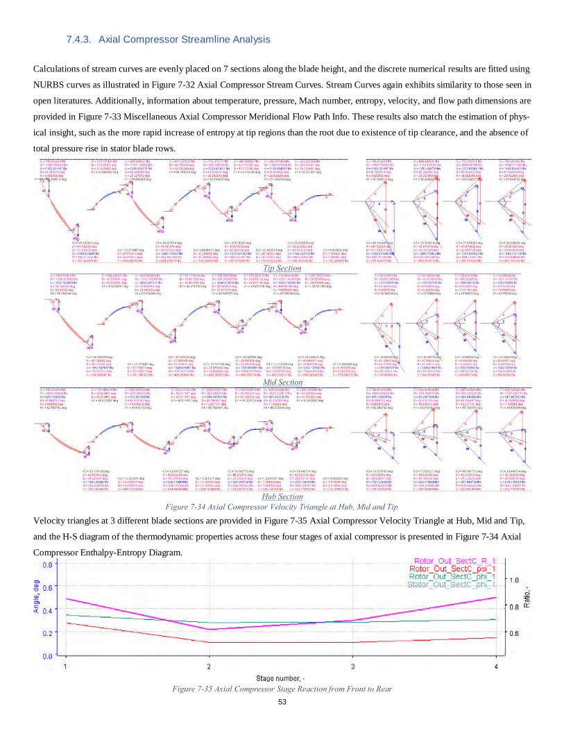
7.4.3. Axial Compressor Streamline Analysis
Calculations of stream curves are evenly placed on 7 sections along the blade height, and the discrete numerical results are fitted using
NURBS curves as illustrated in Figure 7-32 Axial Compressor Stream Curves. Stream Curves again exhibits similarity to those seen in
open literatures. Additionally, information about temperature, pressure, Mach number, entropy, velocity, and flow path dimensions are
provided in Figure 7-33 Miscellaneous Axial Compressor Meridional Flow Path Info. These results also match the estimation of phys-
ical insight, such as the more rapid increase of entropy at tip regions than the root due to existence of tip clearance, and the absence of
total pressure rise in stator blade rows.
Velocity triangles at 3 different blade sections are provided in Figure 7-35 Axial Compressor Velocity Triangle at Hub, Mid and Tip,
and the H-S diagram of the thermodynamic properties across these four stages of axial compressor is presented in Figure 7-34 Axial
Compressor Enthalpy-Entropy Diagram.
Figure 7-35 Axial Compressor Stage Reaction from Front to Rear
Tip Section
Mid Section
Hub Section Figure 7-34 Axial Compressor Velocity Triangle at Hub, Mid and Tip
53
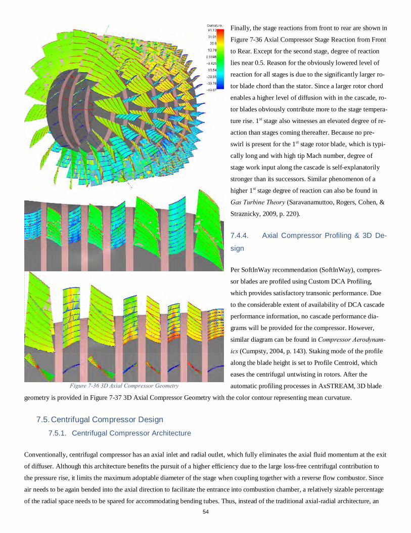
Finally, the stage reactions from front to rear are shown in
Figure 7-36 Axial Compressor Stage Reaction from Front
to Rear. Except for the second stage, degree of reaction
lies near 0.5. Reason for the obviously lowered level of
reaction for all stages is due to the significantly larger ro-
tor blade chord than the stator. Since a larger rotor chord
enables a higher level of diffusion with in the cascade, ro-
tor blades obviously contribute more to the stage tempera-
ture rise. 1st stage also witnesses an elevated degree of re-
action than stages coming thereafter. Because no pre-
swirl is present for the 1st stage rotor blade, which is typi-
cally long and with high tip Mach number, degree of
stage work input along the cascade is self-explanatorily
stronger than its successors. Similar phenomenon of a
higher 1st stage degree of reaction can also be found in
Gas Turbine Theory (Saravanamuttoo, Rogers, Cohen, &
Straznicky, 2009, p. 220).
7.4.4. Axial Compressor Profiling & 3D De-
sign
Per SoftInWay recommendation (SoftInWay), compres-
sor blades are profiled using Custom DCA Profiling,
which provides satisfactory transonic performance. Due
to the considerable extent of availability of DCA cascade
performance information, no cascade performance dia-
grams will be provided for the compressor. However,
similar diagram can be found in Compressor Aerodynam-
ics (Cumpsty, 2004, p. 143). Staking mode of the profile
along the blade height is set to Profile Centroid, which
eases the centrifugal untwisting in rotors. After the
automatic profiling processes in AxSTREAM, 3D blade
geometry is provided in Figure 7-37 3D Axial Compressor Geometry with the color contour representing mean curvature.
7.5. Centrifugal Compressor Design 7.5.1. Centrifugal Compressor Architecture
Conventionally, centrifugal compressor has an axial inlet and radial outlet, which fully eliminates the axial fluid momentum at the exit
of diffuser. Although this architecture benefits the pursuit of a higher efficiency due to the large loss-free centrifugal contribution to
the pressure rise, it limits the maximum adoptable diameter of the stage when coupling together with a reverse flow combustor. Since
air needs to be again bended into the axial direction to facilitate the entrance into combustion chamber, a relatively sizable percentage
of the radial space needs to be spared for accommodating bending tubes. Thus, instead of the traditional axial-radial architecture, an
Figure 7-36 3D Axial Compressor Geometry
54
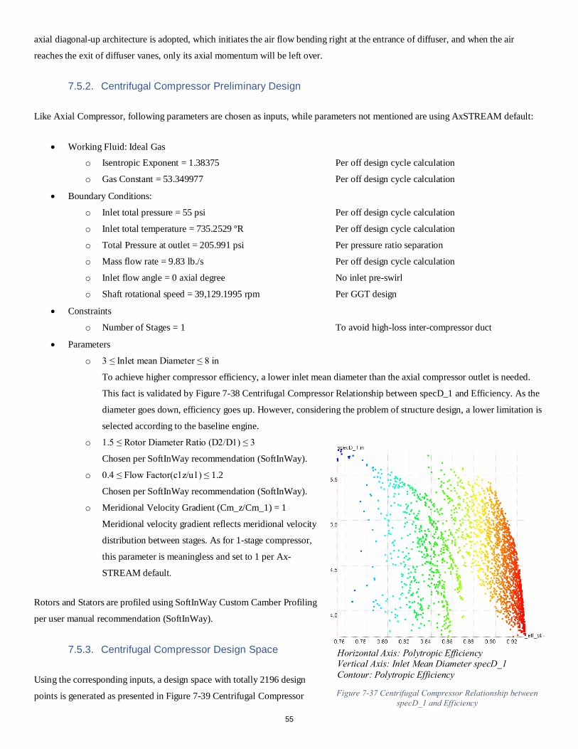
axial diagonal-up architecture is adopted, which initiates the air flow bending right at the entrance of diffuser, and when the air
reaches the exit of diffuser vanes, only its axial momentum will be left over.
7.5.2. Centrifugal Compressor Preliminary Design
Like Axial Compressor, following parameters are chosen as inputs, while parameters not mentioned are using AxSTREAM default:
• Working Fluid: Ideal Gas
o Isentropic Exponent = 1.38375 Per off design cycle calculation
o Gas Constant = 53.349977 Per off design cycle calculation
• Boundary Conditions:
o Inlet total pressure = 55 psi Per off design cycle calculation
o Inlet total temperature = 735.2529 ºR Per off design cycle calculation
o Total Pressure at outlet = 205.991 psi Per pressure ratio separation
o Mass flow rate = 9.83 lb./s Per off design cycle calculation
o Inlet flow angle = 0 axial degree No inlet pre-swirl
o Shaft rotational speed = 39,129.1995 rpm Per GGT design
• Constraints
o Number of Stages = 1 To avoid high-loss inter-compressor duct
• Parameters
o 3 ≤ Inlet mean Diameter ≤ 8 in
To achieve higher compressor efficiency, a lower inlet mean diameter than the axial compressor outlet is needed.
This fact is validated by Figure 7-38 Centrifugal Compressor Relationship between specD_1 and Efficiency. As the
diameter goes down, efficiency goes up. However, considering the problem of structure design, a lower limitation is
selected according to the baseline engine.
o 1.5 ≤ Rotor Diameter Ratio (D2/D1) ≤ 3
Chosen per SoftInWay recommendation (SoftInWay).
o 0.4 ≤ Flow Factor(c1z/u1) ≤ 1.2
Chosen per SoftInWay recommendation (SoftInWay).
o Meridional Velocity Gradient (Cm_z/Cm_1) = 1
Meridional velocity gradient reflects meridional velocity
distribution between stages. As for 1-stage compressor,
this parameter is meaningless and set to 1 per Ax-
STREAM default.
Rotors and Stators are profiled using SoftInWay Custom Camber Profiling
per user manual recommendation (SoftInWay).
7.5.3. Centrifugal Compressor Design Space
Using the corresponding inputs, a design space with totally 2196 design
points is generated as presented in Figure 7-39 Centrifugal Compressor
Horizontal Axis: Polytropic Efficiency Vertical Axis: Inlet Mean Diameter specD_1 Contour: Polytropic Efficiency
Figure 7-37 Centrifugal Compressor Relationship between specD_1 and Efficiency
55
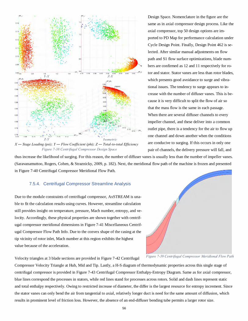
Design Space. Nomenclature in the figure are the
same as in axial compressor design process. Like the
axial compressor, top 50 design options are im-
ported to PD Map for performance calculation under
Cycle Design Point. Finally, Design Point 462 is se-
lected. After similar manual adjustments on flow
path and S1 flow surface optimizations, blade num-
bers are confirmed as 12 and 11 respectively for ro-
tor and stator. Stator vanes are less than rotor blades,
which presents good avoidance to surge and vibra-
tional issues. The tendency to surge appears to in-
crease with the number of diffuser vanes. This is be-
cause it is very difficult to split the flow of air so
that the mass flow is the same in each passage.
When there are several diffuser channels to every
impeller channel, and these deliver into a common
outlet pipe, there is a tendency for the air to flow up
one channel and down another when the conditions
are conducive to surging. If this occurs in only one
pair of channels, the delivery pressure will fall, and
thus increase the likelihood of surging. For this reason, the number of diffuser vanes is usually less than the number of impeller vanes.
(Saravanamuttoo, Rogers, Cohen, & Straznicky, 2009, p. 182). Next, the meridional flow path of the machine is frozen and presented
in Figure 7-40 Centrifugal Compressor Meridional Flow Path.
7.5.4. Centrifugal Compressor Streamline Analysis
Due to the module constraints of centrifugal compressor, AxSTREAM is una-
ble to fit the calculation results using curves. However, streamline calculation
still provides insight on temperature, pressure, Mach number, entropy, and ve-
locity. Accordingly, these physical properties are shown together with centrif-
ugal compressor meridional dimensions in Figure 7-41 Miscellaneous Centrif-
ugal Compressor Flow Path Info. Due to the convex shape of the casing at the
tip vicinity of rotor inlet, Mach number at this region exhibits the highest
value because of the acceleration.
Velocity triangles at 3 blade sections are provided in Figure 7-42 Centrifugal
Compressor Velocity Triangle at Hub, Mid and Tip. Lastly, a H-S diagram of thermodynamic properties across this single stage of
centrifugal compressor is provided in Figure 7-43 Centrifugal Compressor Enthalpy-Entropy Diagram. Same as for axial compressor,
blue lines correspond the processes in stators, while red lines stand for processes across rotors. Solid and dash lines represent static
and total enthalpy respectively. Owing to restricted increase of diameter, the differ is the largest resource for entropy increment. Since
the stator vanes can only bend the air from tangential to axial, relatively longer duct is need for the same amount of diffusion, which
results in prominent level of friction loss. However, the absence of an end-diffuser bending tube permits a larger rotor size.
Y-X
Z-Y
Z-X
IsometricX ― Stage Loading (psi); Y ― Flow Coefficient (phi); Z ― Total-to-total Efficiency
(Eff tt) Figure 7-38 Centrifugal Compressor Design Space
Figure 7-39 Centrifugal Compressor Meridional Flow Path
56
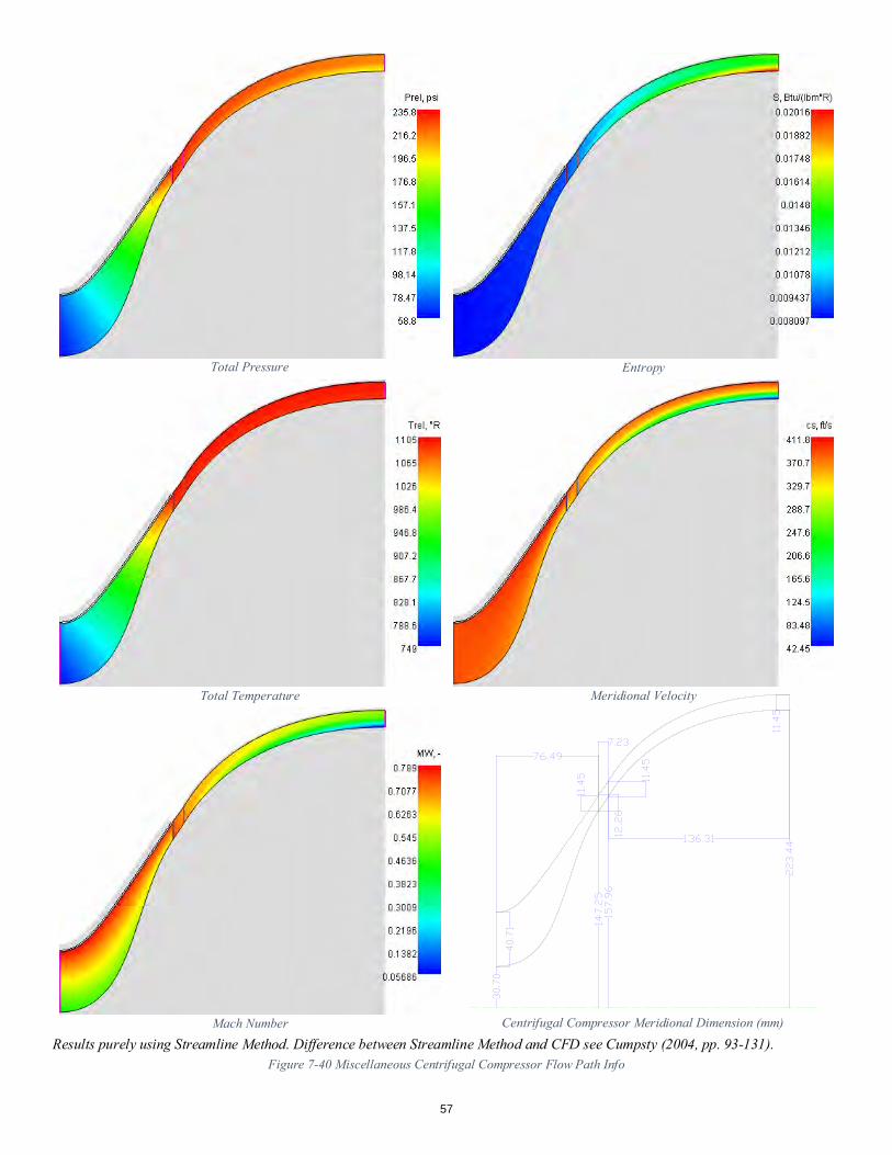
Centrifugal Compressor Meridional Dimension (mm)
Total Pressure
Total Temperature
Entropy
Meridional Velocity
Mach Number Results purely using Streamline Method. Difference between Streamline Method and CFD see Cumpsty (2004, pp. 93-131).
Figure 7-40 Miscellaneous Centrifugal Compressor Flow Path Info
57
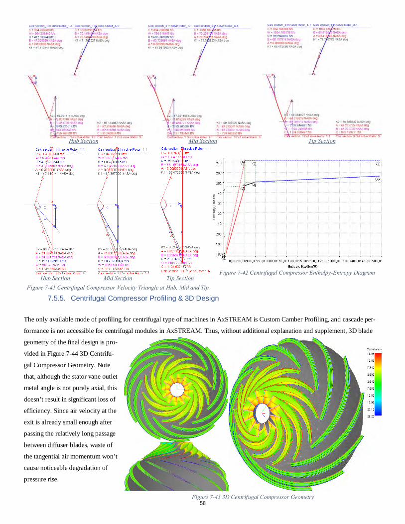
7.5.5. Centrifugal Compressor Profiling & 3D Design
The only available mode of profiling for centrifugal type of machines in AxSTREAM is Custom Camber Profiling, and cascade per-
formance is not accessible for centrifugal modules in AxSTREAM. Thus, without additional explanation and supplement, 3D blade
geometry of the final design is pro-
vided in Figure 7-44 3D Centrifu-
gal Compressor Geometry. Note
that, although the stator vane outlet
metal angle is not purely axial, this
doesn’t result in significant loss of
efficiency. Since air velocity at the
exit is already small enough after
passing the relatively long passage
between diffuser blades, waste of
the tangential air momentum won’t
cause noticeable degradation of
pressure rise.
Figure 7-42 Centrifugal Compressor Enthalpy-Entropy Diagram
Figure 7-41 Centrifugal Compressor Velocity Triangle at Hub, Mid and Tip
Tip Section Hub Section Mid Section
Tip Section Hub Section Mid Section
Figure 7-43 3D Centrifugal Compressor Geometry 58
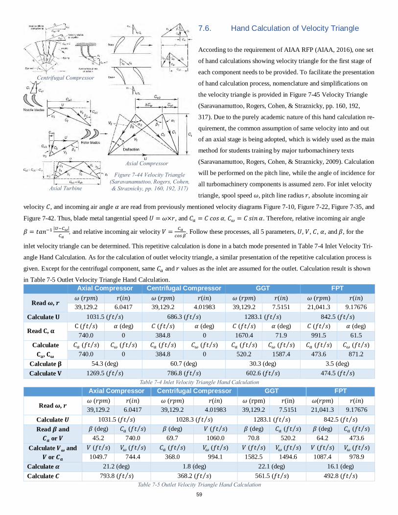
7.6. Hand Calculation of Velocity Triangle
According to the requirement of AIAA RFP (AIAA, 2016), one set
of hand calculations showing velocity triangle for the first stage of
each component needs to be provided. To facilitate the presentation
of hand calculation process, nomenclature and simplifications on
the velocity triangle is provided in Figure 7-45 Velocity Triangle
(Saravanamuttoo, Rogers, Cohen, & Straznicky, pp. 160, 192,
317). Due to the purely academic nature of this hand calculation re-
quirement, the common assumption of same velocity into and out
of an axial stage is being adopted, which is widely used as the main
method for students training by major turbomachinery texts
(Saravanamuttoo, Rogers, Cohen, & Straznicky, 2009). Calculation
will be performed on the pitch line, while the angle of incidence for
all turbomachinery components is assumed zero. For inlet velocity
triangle, spool speed 𝜔𝜔, pitch line radius 𝑟𝑟, absolute incoming air
velocity 𝐶𝐶, and incoming air angle 𝛼𝛼 are read from previously mentioned velocity diagrams Figure 7-10, Figure 7-22, Figure 7-35, and
Figure 7-42. Thus, blade metal tangential speed 𝑈𝑈 = 𝜔𝜔×𝑟𝑟, and 𝐶𝐶𝐴𝐴 = 𝐶𝐶 𝑠𝑠𝑠𝑠𝑠𝑠 𝛼𝛼, 𝐶𝐶𝜔𝜔 = 𝐶𝐶 𝑠𝑠𝑖𝑖𝑠𝑠 𝛼𝛼. Therefore, relative incoming air angle
𝛽𝛽 = 𝑎𝑎𝑎𝑎𝑠𝑠−1 |𝑈𝑈−𝑆𝑆𝜔𝜔|𝑆𝑆𝑚𝑚
, and relative incoming air velocity 𝑉𝑉 = 𝑆𝑆𝑚𝑚𝑉𝑉𝑉𝑉𝑐𝑐𝛽𝛽
. Follow these processes, all 5 parameters, 𝑈𝑈, 𝑉𝑉, 𝐶𝐶, 𝛼𝛼, and 𝛽𝛽, for the
inlet velocity triangle can be determined. This repetitive calculation is done in a batch mode presented in Table 7-4 Inlet Velocity Tri-
angle Hand Calculation. As for the calculation of outlet velocity triangle, a similar presentation of the repetitive calculation process is
given. Except for the centrifugal component, same 𝐶𝐶𝐴𝐴 and 𝑟𝑟 values as the inlet are assumed for the outlet. Calculation result is shown
in Table 7-5 Outlet Velocity Triangle Hand Calculation. Axial Compressor Centrifugal Compressor GGT FPT
Read 𝝎𝝎, 𝒓𝒓 𝜔𝜔 (𝑟𝑟𝑝𝑝𝑎𝑎) 𝑟𝑟(𝑖𝑖𝑠𝑠) 𝜔𝜔 (𝑟𝑟𝑝𝑝𝑎𝑎) 𝑟𝑟(𝑖𝑖𝑠𝑠) 𝜔𝜔 (𝑟𝑟𝑝𝑝𝑎𝑎) 𝑟𝑟(𝑖𝑖𝑠𝑠) 𝜔𝜔 (𝑟𝑟𝑝𝑝𝑎𝑎) 𝑟𝑟(𝑖𝑖𝑠𝑠) 39,129.2 6.0417 39,129.2 4.01983 39,129.2 7.5151 21,041.3 9.17676
Calculate 𝐔𝐔 1031.5 (𝑓𝑓𝑎𝑎 𝑠𝑠⁄ ) 686.3 (𝑓𝑓𝑎𝑎 𝑠𝑠⁄ ) 1283.1 (𝑓𝑓𝑎𝑎 𝑠𝑠⁄ ) 842.5 (𝑓𝑓𝑎𝑎 𝑠𝑠⁄ )
Read 𝐂𝐂, 𝛂𝛂 C (𝑓𝑓𝑎𝑎 𝑠𝑠⁄ ) 𝛼𝛼 (deg) 𝐶𝐶 (𝑓𝑓𝑎𝑎 𝑠𝑠⁄ ) 𝛼𝛼 (deg) 𝐶𝐶 (𝑓𝑓𝑎𝑎 𝑠𝑠⁄ ) 𝛼𝛼 (deg) 𝐶𝐶 (𝑓𝑓𝑎𝑎 𝑠𝑠⁄ ) 𝛼𝛼 (deg)
740.0 0 384.8 0 1670.4 71.9 991.5 61.5 Calculate 𝐂𝐂𝐦𝐦, 𝐂𝐂𝛚𝛚
𝐶𝐶𝐴𝐴 (𝑓𝑓𝑎𝑎 𝑠𝑠⁄ ) 𝐶𝐶𝜔𝜔 (𝑓𝑓𝑎𝑎 𝑠𝑠⁄ ) 𝐶𝐶𝐴𝐴 (𝑓𝑓𝑎𝑎 𝑠𝑠⁄ ) 𝐶𝐶𝜔𝜔 (𝑓𝑓𝑎𝑎 𝑠𝑠⁄ ) 𝐶𝐶𝐴𝐴 (𝑓𝑓𝑎𝑎 𝑠𝑠⁄ ) 𝐶𝐶𝜔𝜔 (𝑓𝑓𝑎𝑎 𝑠𝑠⁄ ) 𝐶𝐶𝐴𝐴 (𝑓𝑓𝑎𝑎 𝑠𝑠⁄ ) 𝐶𝐶𝜔𝜔 (𝑓𝑓𝑎𝑎 𝑠𝑠⁄ ) 740.0 0 384.8 0 520.2 1587.4 473.6 871.2
Calculate 𝛃𝛃 54.3 (deg) 60.7 (deg) 30.3 (deg) 3.5 (deg) Calculate 𝐕𝐕 1269.5 (𝑓𝑓𝑎𝑎 𝑠𝑠⁄ ) 786.8 (𝑓𝑓𝑎𝑎 𝑠𝑠⁄ ) 602.6 (𝑓𝑓𝑎𝑎 𝑠𝑠⁄ ) 474.5 (𝑓𝑓𝑎𝑎 𝑠𝑠⁄ )
Table 7-4 Inlet Velocity Triangle Hand Calculation Axial Compressor Centrifugal Compressor GGT FPT
Read 𝝎𝝎, 𝒓𝒓 𝜔𝜔 (𝑟𝑟𝑝𝑝𝑎𝑎) 𝑟𝑟(𝑖𝑖𝑠𝑠) 𝜔𝜔 (𝑟𝑟𝑝𝑝𝑎𝑎) 𝑟𝑟(𝑖𝑖𝑠𝑠) 𝜔𝜔 (rpm) 𝑟𝑟(in) 𝜔𝜔(𝑟𝑟𝑝𝑝𝑎𝑎) 𝑟𝑟(𝑖𝑖𝑠𝑠) 39,129.2 6.0417 39,129.2 4.01983 39,129.2 7.5151 21,041.3 9.17676
Calculate 𝑼𝑼 1031.5 (𝑓𝑓𝑎𝑎 𝑠𝑠⁄ ) 1028.3 (𝑓𝑓𝑎𝑎 𝑠𝑠⁄ ) 1283.1 (𝑓𝑓𝑎𝑎 𝑠𝑠⁄ ) 842.5 (𝑓𝑓𝑎𝑎 𝑠𝑠⁄ ) Read 𝜷𝜷 and 𝑪𝑪𝒂𝒂 or 𝑽𝑽
𝛽𝛽 (deg) 𝐶𝐶𝐴𝐴 (𝑓𝑓𝑎𝑎 𝑠𝑠⁄ ) 𝛽𝛽 (deg) 𝑉𝑉 (𝑓𝑓𝑎𝑎 𝑠𝑠⁄ ) 𝛽𝛽 (deg) 𝐶𝐶𝐴𝐴 (𝑓𝑓𝑎𝑎 𝑠𝑠⁄ ) 𝛽𝛽 (deg) 𝐶𝐶𝐴𝐴 (𝑓𝑓𝑎𝑎 𝑠𝑠⁄ ) 45.2 740.0 69.7 1060.0 70.8 520.2 64.2 473.6
Calculate 𝑽𝑽𝝎𝝎 and 𝑽𝑽 or 𝑪𝑪𝒂𝒂
𝑉𝑉 (𝑓𝑓𝑎𝑎 𝑠𝑠⁄ ) 𝑉𝑉𝜔𝜔 (𝑓𝑓𝑎𝑎 𝑠𝑠⁄ ) 𝐶𝐶𝐴𝐴 (𝑓𝑓𝑎𝑎 𝑠𝑠⁄ ) 𝑉𝑉𝜔𝜔 (𝑓𝑓𝑎𝑎 𝑠𝑠⁄ ) 𝑉𝑉 (𝑓𝑓𝑎𝑎 𝑠𝑠⁄ ) 𝑉𝑉𝜔𝜔 (𝑓𝑓𝑎𝑎 𝑠𝑠⁄ ) 𝑉𝑉 (𝑓𝑓𝑎𝑎 𝑠𝑠⁄ ) 𝑉𝑉𝜔𝜔 (𝑓𝑓𝑎𝑎 𝑠𝑠⁄ ) 1049.7 744.4 368.0 994.1 1582.5 1494.6 1087.4 978.9
Calculate 𝜶𝜶 21.2 (deg) 1.8 (deg) 22.1 (deg) 16.1 (deg) Calculate 𝑪𝑪 793.8 (𝑓𝑓𝑎𝑎 𝑠𝑠⁄ ) 368.2 (𝑓𝑓𝑎𝑎 𝑠𝑠⁄ ) 561.5 (𝑓𝑓𝑎𝑎 𝑠𝑠⁄ ) 492.8 (𝑓𝑓𝑎𝑎 𝑠𝑠⁄ )
Table 7-5 Outlet Velocity Triangle Hand Calculation
Axial Compressor
Axial Turbine
Centrifugal Compressor
Figure 7-44 Velocity Triangle (Saravanamuttoo, Rogers, Cohen, & Straznicky, pp. 160, 192, 317)
59
Note that the hand calculation of the outlet velocity triangle shows a very small value of 𝛼𝛼 for centrifugal compressor, which corre-
sponds to nearly pure axial outlet air direction and absence of tangential momentum at Turbomachinery Design Point. Since the spatial
velocity triangle is not projected on to a plane parallel to the rotation axis, the shape of the hand calculated velocity triangle may differ
from that generated by AxSTREAM for the centrifugal compressor.
7.7. Detailed Component Information
Due the extensive number of parameters involved in AxSTREAM for defining the 3D geometry of the turbomachinery design out-
come, it is not possible to include all of them in this proposal. Therefore, only those geometrical parameters required by the RFP are
presented in Table 7-7 Axial Compressor Detailed Information, Table 7-6 Centrifugal Compressor Detailed Information, Table 7-8
GGT Detailed Information, and Table 7-9 FPT Detailed Information respectively. Angles are defined as Figure 7-45 Velocity Triangle
(Saravanamuttoo, Rogers, Cohen, & Straznicky, pp. 160, 192, 317) RPF Nomenclature Nomenclature in AxSTREAM Units Machine Level Rotor diagonal 1-1 Stator diagonal 3-1
Lieblein Diffusion Factor -- -- Not available for centrifugal components De Haller Number -- -- Not available for centrifugal components
Stage Loading averaged work coefficient (H/U2^2) -- 0.524864 0.524864 -- Flow Coefficient averaged flow coefficient (C2s/U2) -- 0.178023 0.178023 --
Hub-to-Tip Ratio mean diameter to blade height ratio -- -- 26.710898 40.012925
-- -- 0.927826229 0.951234885 Number of Blades (Rotor & Stator) number of blades -- -- 12 11
Solidity Solidity -- Tip 9.111363 1.544967 -- Mid 12.537166 1.599023 -- Hub 20.597461 1.656999
Pitch cascade pitch in Tip 1.47196 3.809891 in Mid 1.052389 3.681094 in Hub 0.632817 3.552297
Chord (Axial & Blade)
chord in Tip 13.411565 5.886154 in Mid 13.193972 5.886154 in Hub 13.034425 5.886154
profile axial chord length in Tip 3.011452 5.36673 in Mid 3.011452 5.36673 in Hub 3.011452 5.36673
Aspect Ratio aspect ratio -- -- 0.121468 0.076615
Taper Ratio -- -- Chord Taper 1.028934149 1 -- -- Axial Taper 1 1
Tip Speed tangential velocity @ Section 3 ft./s -- 959.9439428 -- Stagger Angle -- -- Not available for centrifugal components
Blade metal angles
inlet metal angle deg Tip 69.466527 71.749009 deg Mid 62.350925 71.749009 deg Hub 48.93692 71.749009
outlet metal angle deg Tip 68.284067 60.360734 deg Mid 67.550521 59.749009 deg Hub 66.768515 59.114035
Velocity Triangles (hub, mean, & tip) Figure 7-42 Centrifugal Compressor Velocity Triangle at Hub, Mid and Tip Degree of Reaction reaction Average 0.807439
Mach Numbers (absolute & relative) Mach number
inlet Average 0.293558 0.678845 outlet Average 0.738158 0.38906
Mach number in rel. frame inlet Average 0.605027 -- outlet Average 0.688316 --
Table 7-6 Centrifugal Compressor Detailed Information
60
RFP Nomenclature Nomenclature in AxSTREAM Units Machine Level
Rotor 1-1
Stator 2-1
Rotor 3-2
Stator 4-2
Rotor 5-3
Stator 6-3
Rotor 7-4
Stator 8-4
Lieblein Diffusion Factor diffusion factor (by NASA) -- Average 0.555285 0.410298 0.447702 0.450719 0.389683 0.462316 0.372392 0.367174 De Haller Number diffusion factor by de Haller (w2/w1) -- Average 0.612132 0.8495 0.712158 0.78104 0.786797 0.788556 0.775019 0.855687
Stage Loading averaged work coefficient (H/U2^2) -- 0.371519 0.480683 -- 0.355192 -- 0.252539 -- 0.301343 -- Flow Coefficient averaged flow coefficient (C2s/U2) -- 0.711678 0.492008 -- 0.561582 -- 0.59488 -- 0.642488 --
Hub-to-Tip Ratio mean diameter to blade height ratio -- -- 3.581322 4.235536 4.785308 5.219834 5.681755 6.293141 7.065301 8.477373
-- -- -- 0.563445 0.617995 0.654297 0.678448 0.700677 0.725770 0.752024 0.788971 Number of Blades number of blades -- -- 18 23 24 29 30 37 36 43
Solidity Solidity -- Tip 1.55379 0.942124 1.532404 0.973463 1.039089 1.001196 1.240335 1.405696 -- Mid 1.023929 0.692578 1.183653 0.775373 0.844927 0.829755 1.050976 1.216574 -- Hub 0.763549 0.547547 0.964214 0.64427 0.711903 0.708443 0.911777 1.072306
Pitch cascade pitch in Tip 0.694887 0.619357 0.623004 0.529266 0.518004 0.42489 0.443384 0.379114 in Mid 1.054477 0.84252 0.806564 0.664482 0.637041 0.512679 0.523271 0.438049 in Hub 1.414066 1.065683 0.990125 0.799698 0.756077 0.600469 0.603157 0.496984
Chord (Axial & Blade)
chord in Tip 1.079709 0.583511 0.954693 0.515221 0.538253 0.425398 0.549945 0.532919 in Mid 1.079709 0.583511 0.954693 0.515221 0.538253 0.425398 0.549945 0.532919 in Hub 1.079709 0.583511 0.954693 0.515221 0.538253 0.425398 0.549945 0.532919
profile axial chord length In Tip 0.934046 0.52168 0.845043 0.466655 0.465095 0.398487 0.457712 0.50011 in Mid 0.747642 0.514763 0.724915 0.432124 0.422305 0.377042 0.42814 0.50327 in Hub 0.618783 0.514738 0.636841 0.409447 0.377316 0.359194 0.39823 0.505011
Aspect Ratio aspect ratio -- -- 1.908194 2.799955 1.468852 2.422604 2.111852 2.430516 1.664589 1.51367
Taper Ratio -- -- Chord Taper 1 1 1 1 1 1 1 1 -- -- Axial Taper 1.5094888 1.0134865 1.3269293 1.1397202 1.2326405 1.1093921 1.1493659 0.9902953
Tip Speed tangential velocity @ Section 3 ft./s -- 1383.2815 -- 1291.4270 -- 1232.6947 -- 1180.0535 --
Stagger Angle stagger angle design deg Hub 30.35245 26.991749 28.052695 25.657887 30.65413 21.187538 34.141884 20.791341 deg Mid 46.574855 28.506069 40.999897 33.424554 38.816769 28.087739 39.427537 19.750533 deg Tip 55.498459 28.511504 48.645839 37.880926 46.104898 32.831587 44.241483 19.151994
Blade metal angles
inlet metal angle deg Hub 42.569792 40.610451 43.410163 48.011557 45.760487 45.209334 48.835054 41.582682 deg Mid 54.344244 43.639091 52.654049 46.47135 48.546953 43.857118 49.056246 39.501066 deg Tip 61.854514 43.649962 58.088665 44.76524 54.534837 43.170196 51.64453 38.303987
outlet metal angle deg Hub 18.135109 13.373047 12.695227 3.304217 15.547772 -2.834257 19.448714 0 deg Mid 38.805465 13.373047 29.345745 20.377758 29.086586 12.318359 29.798828 0 deg Tip 49.142405 13.373047 39.203014 30.996612 37.67496 22.492979 36.838436 0
Velocity Triangles Figure 7-35 Axial Compressor Velocity Triangle at Hub, Mid and Tip Degree of Reaction reaction Average 0.890648 0.890648 0.63488 0.63488
Mach Numbers (absolute & rel-ative)
Mach number inlet Average 0.697214 0.659892 0.57388 0.730448 0.574229 0.698691 0.563483 0.686789 outlet Average 0.642829 0.555522 0.719278 0.560818 0.687094 0.542608 0.666494 0.581333
Mach number in rel. frame inlet Average 1.203259 -- 0.885647 -- 0.781571 -- 0.812936 -- outlet Average 0.674272 -- 0.612048 -- 0.602968 -- 0.616288 -- Table 7-7 Axial Compressor Detailed Information
61
RFP Nomenclature Nomenclature in Ax-
STREAM Units Machine Level
Stator 1-1
Rotor 2-1
Stator 3-2
Rotor 4-2
Zweifel Coefficient Zweifel Coefficient -- -- 0.761028 0.477893 0.527248 0.572412
Taper Ratio -- -- Chord Taper 1 1 1 1
-- -- Axial Taper 1 0.6802955 0.8176782 0.5055325
Stage Work power Btu/s 1778.925336 884.04841 894.876926
Stage Pressure Ratio total-total pressure ratio --
4.382996 1.99147 2.240771
-- 1.018073 1.923846 1.021185 2.200306
Degree of Reaction reaction -- Average 0.446557 0.471717
Velocity Triangle Figure 7-10 GGT Velocity Triangle at Hub, Mid, and Tip
Aspect Ratio aspect ratio -- -- 0.85473 2.198609 1.449293 3.55094
AN2
tip diameter at inlet in -- 8.004614 8.402466 8.662011 9.267517
hub diameter at inlet in -- 7.025586 6.964468 6.904702 6.728763
tip diameter at outlet in -- 8.291202 8.559964 9.04353 9.424
hub diameter at outlet in -- 7.025586 6.978706 6.912097 6.606
shaft rotational speed rpm 39129.1955 -- -- -- --
-- in2rpm2 -- -- 1.12. E+11 -- 2.06. E+11
Number of Blades number of blades -- -- 41 88 43 90
Chord (Axial & Blade)
chord
in Tip 0.767784 0.374752 0.786979 0.396796
in Mid 0.767784 0.374752 0.786979 0.396796
in Hub 0.767784 0.374752 0.786979 0.396796
profile axial chord length
in Tip 0.472817 0.234306 0.521211 0.189602
in Mid 0.472817 0.302212 0.588735 0.303754
in Hub 0.472817 0.344418 0.637428 0.375054
Blade Metal Angles
inlet metal angle
deg Tip 0.000013 0.150436 -7.175687 -28.379557
deg Mid 0.000013 28.656655 -20.23922 20.639045
deg Hub 0.000013 46.389686 -29.28848 49.608009
outlet metal angle
deg Tip 71.423719 -70.809425 71.281586 -69.723334
deg Mid 71.423719 -70.809425 71.281586 -69.723334
deg Hub 71.423719 -70.809425 71.281586 -69.723334
Mach numbers (abso-
lute and relative)
Mach number inlet Average 0.242091 0.745659 0.259015 0.790585
outlet Average 0.756436 0.274781 0.806982 0.332176
Mach number in rel. frame inlet Average -- 0.262012 -- 0.289624
outlet Average -- 0.766003 -- 0.872249
Tip speed tangential velocity @ Section 3 ft./s -- -- 1434.575274 -- 1267.349103
Flow Coefficient averaged flow coefficient
(C2s/U2) -- 0.409121 -- 0.403914 -- 0.429251
Stage Work Split -- -- -- 0.496956444494644:0.503043555505356
Pitch cascade pitch
in Tip 0.635307 0.30559 0.660723 0.32896
in Mid 0.585022 0.276176 0.577393 0.279776
in Hub 0.534738 0.246761 0.494063 0.230593
Cooling Flow Details GGT Uncooled
Table 7-8 GGT Detailed Information
62
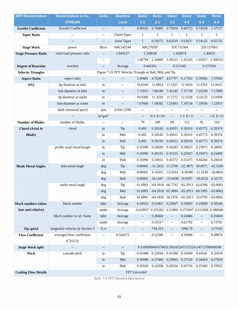
RFP Nomenclature Nomenclature in Ax-STREAM
Units Machine Level
Stator 1-1
Rotor 2-1
Stator 3-2
Rotor 4-2
Stator 5-3
Rotor 6-3
Zweifel Coefficient Zweifel Coefficient -- -- 0.90526 0.76800 0.75034 0.84723 0.74328 1.37157
Taper Ratio -- -- Chord Taper 1 1 1 1 1 1
-- -- Axial Taper 1 0.59272 0.63229 0.63627 0.54132 0.65735
Stage Work power Btu/s 948.145244 300.276597 318.731584 329.137063
Stage Pressure Ratio total-total pressure ratio -- 2.844227 1.358658 1.420074 1.49433
-- 1.00794 1.34889 1.00513 1.41243 1.01057 1.368163
Degree of Reaction reaction -- Average 0.442161 0.515542 0.571916
Velocity Triangles Figure 7-22 FPT Velocity Triangle at Hub, Mid, and Tip
Aspect Ratio aspect ratio -- -- 3.30681 4.76387 4.67707 6.17592 5.76992 7.37842
AN2 tip diameter at inlet in -- 10.6244 11.0054 11.5321 11.9454 12.4763 12.8423
hub diameter at inlet in -- 7.72913 7.60189 7.45145 7.37739 7.25258 7.17889
tip diameter at outlet in -- 10.9306 11.3220 11.7272 12.2528 12.6122 13.0394
hub diameter at outlet in -- 7.67668 7.58282 7.51683 7.39734 7.33026 7.22913
shaft rotational speed rpm 21041.2598 -- -- -- -- -- --
-- in2rpm2 -- 9.3. E+10 -- 1.3. E+11 -- 1.6. E+11
Number of Blades number of blades -- -- 79 108 89 112 91 114
Chord (Axial &
Blade)
chord in Tip 0.492 0.39245 0.45011 0.39310 0.45772 0.39374
in Mid 0.492 0.39245 0.45011 0.39310 0.45772 0.39374
in Hub 0.492 0.39245 0.45011 0.39310 0.45772 0.39374
profile axial chord length in Tip 0.35096 0.20699 0.26285 0.20025 0.23972 0.18691
in Mid 0.35096 0.28155 0.35155 0.25927 0.35973 0.23400
in Hub 0.35096 0.34922 0.41572 0.31473 0.44284 0.28434
Blade Metal Angles inlet metal angle deg Tip 0.00001 -31.2632 15.5790 -32.3875 30.0071 -42.5169
deg Mid 0.00001 4.16931 -12.9161 -4.38380 -11.3149 -18.8854
deg Hub 0.00001 34.1447 -33.0430 19.9597 -39.6532 4.32175
outlet metal angle deg Tip 61.6991 -64.1818 66.7742 -65.2913 65.6394 -63.8062
deg Mid 61.6991 -64.1818 62.3894 -65.2913 60.1995 -63.8062
deg Hub 61.6991 -64.1818 56.1976 -65.2913 52.0793 -63.8062
Mach numbers (abso-
lute and relative)
Mach number inlet Average 0.24933 0.51803 0.23607 0.50843 0.25699 0.50146
outlet Average 0.618957 0.255262 0.51869 0.272607 0.511669 0.386846
Mach number in rel. frame inlet Average -- 0.26660 -- 0.24466 -- 0.26844
outlet Average -- 0.55317 -- 0.61792 -- 0.73781
Tip speed tangential velocity @ Section 3 ft./s -- -- 734.313 -- 1096.70 -- 1179.05
Flow Coefficient averaged flow coefficient
(C2s/U2)
-- 0.542675 -- 0.52506 -- 0.50888 -- 0.49874
Stage Work Split -- -- -- 0.31669894343740:0.33616324715752:0.34713780940508
Pitch cascade pitch in Tip 0.43468 0.32934 0.41396 0.34369 0.43541 0.35934
in Mid 0.36998 0.27496 0.33965 0.27559 0.34424 0.27928
in Hub 0.30528 0.22058 0.26534 0.20750 0.25306 0.19922
Cooling Flow Details FPT Uncooled
Table 7-9 FPT Detailed Information
63
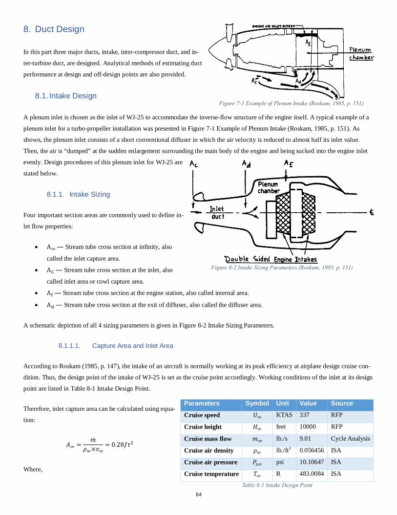
8. Duct Design
In this part three major ducts, intake, inter-compressor duct, and in-
ter-turbine duct, are designed. Analytical methods of estimating duct
performance at design and off-design points are also provided.
8.1. Intake Design
A plenum inlet is chosen as the inlet of WJ-25 to accommodate the inverse-flow structure of the engine itself. A typical example of a
plenum inlet for a turbo-propeller installation was presented in Figure 7-1 Example of Plenum Intake (Roskam, 1985, p. 151). As
shown, the plenum inlet consists of a short conventional diffuser in which the air velocity is reduced to almost half its inlet value.
Then, the air is “dumped” at the sudden enlargement surrounding the main body of the engine and being sucked into the engine inlet
evenly. Design procedures of this plenum inlet for WJ-25 are
stated below.
8.1.1. Intake Sizing
Four important section areas are commonly used to define in-
let flow properties:
• A∞ ― Stream tube cross section at infinity, also
called the inlet capture area.
• AC ― Stream tube cross section at the inlet, also
called inlet area or cowl capture area.
• Af ― Stream tube cross section at the engine station, also called internal area.
• Ad ― Stream tube cross section at the exit of diffuser, also called the diffuser area.
A schematic depiction of all 4 sizing parameters is given in Figure 8-2 Intake Sizing Parameters.
8.1.1.1. Capture Area and Inlet Area
According to Roskam (1985, p. 147), the intake of an aircraft is normally working at its peak efficiency at airplane design cruise con-
dition. Thus, the design point of the intake of WJ-25 is set as the cruise point accordingly. Working conditions of the inlet at its design
point are listed in Table 8-1 Intake Design Point.
Therefore, inlet capture area can be calculated using equa-
tion:
𝐴𝐴∞ =�̇�𝑎
𝜌𝜌∞×𝑣𝑣∞= 0.28𝑓𝑓𝑎𝑎2
Where,
Parameters Symbol Unit Value Source Cruise speed 𝑈𝑈∞ KTAS 337 RFP
Cruise height 𝑆𝑆∞ feet 10000 RFP
Cruise mass flow 𝑎𝑎∞ lb./s 9.01 Cycle Analysis
Cruise air density 𝜌𝜌∞ lb./ft3 0.056456 ISA
Cruise air pressure 𝑃𝑃𝑐𝑐∞ psi 10.10647 ISA
Cruise temperature 𝑂𝑂∞ R 483.0084 ISA
Table 8-1 Intake Design Point
Figure 7-1 Example of Plenum Intake (Roskam, 1985, p. 151)
Figure 8-2 Intake Sizing Parameters (Roskam, 1985, p. 151)
64
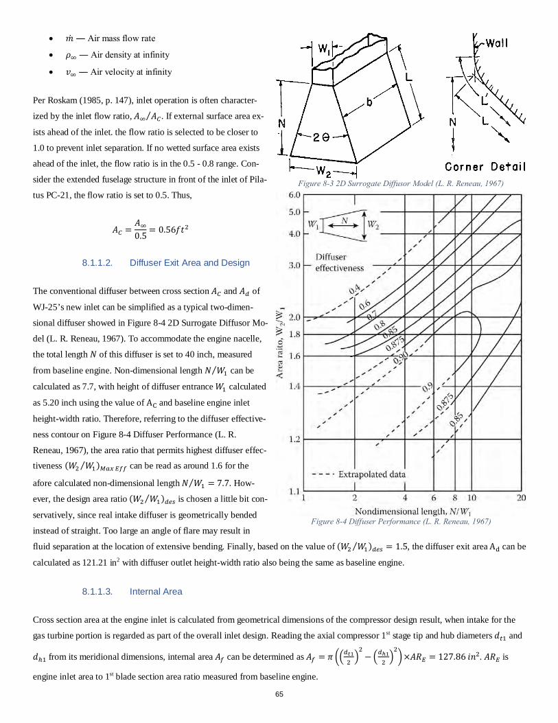
• �̇�𝑎 ― Air mass flow rate
• 𝜌𝜌∞ ― Air density at infinity
• 𝑣𝑣∞ ― Air velocity at infinity
Per Roskam (1985, p. 147), inlet operation is often character-
ized by the inlet flow ratio, 𝐴𝐴∞ 𝐴𝐴𝑆𝑆⁄ . If external surface area ex-
ists ahead of the inlet. the flow ratio is selected to be closer to
1.0 to prevent inlet separation. If no wetted surface area exists
ahead of the inlet, the flow ratio is in the 0.5 - 0.8 range. Con-
sider the extended fuselage structure in front of the inlet of Pila-
tus PC-21, the flow ratio is set to 0.5. Thus,
𝐴𝐴𝑆𝑆 =𝐴𝐴∞0.5 = 0.56𝑓𝑓𝑎𝑎2
8.1.1.2. Diffuser Exit Area and Design
The conventional diffuser between cross section 𝐴𝐴𝑆𝑆 and 𝐴𝐴𝑑𝑑 of
WJ-25’s new inlet can be simplified as a typical two-dimen-
sional diffuser showed in Figure 8-4 2D Surrogate Diffusor Mo-
del (L. R. Reneau, 1967). To accommodate the engine nacelle,
the total length 𝑁𝑁 of this diffuser is set to 40 inch, measured
from baseline engine. Non-dimensional length 𝑁𝑁 𝑘𝑘1⁄ can be
calculated as 7.7, with height of diffuser entrance 𝑘𝑘1 calculated
as 5.20 inch using the value of AC and baseline engine inlet
height-width ratio. Therefore, referring to the diffuser effective-
ness contour on Figure 8-4 Diffuser Performance (L. R.
Reneau, 1967), the area ratio that permits highest diffuser effec-
tiveness (𝑘𝑘2 𝑘𝑘1⁄ )𝑀𝑀𝐴𝐴𝐸𝐸 𝐸𝐸𝑟𝑟𝑟𝑟 can be read as around 1.6 for the
afore calculated non-dimensional length 𝑁𝑁 𝑘𝑘1⁄ = 7.7. How-
ever, the design area ratio (𝑘𝑘2 𝑘𝑘1⁄ )𝑑𝑑𝑉𝑉𝑐𝑐 is chosen a little bit con-
servatively, since real intake diffuser is geometrically bended
instead of straight. Too large an angle of flare may result in
fluid separation at the location of extensive bending. Finally, based on the value of (𝑘𝑘2 𝑘𝑘1⁄ )𝑑𝑑𝑉𝑉𝑐𝑐 = 1.5, the diffuser exit area Ad can be
calculated as 121.21 in2 with diffuser outlet height-width ratio also being the same as baseline engine.
8.1.1.3. Internal Area
Cross section area at the engine inlet is calculated from geometrical dimensions of the compressor design result, when intake for the
gas turbine portion is regarded as part of the overall inlet design. Reading the axial compressor 1st stage tip and hub diameters 𝑠𝑠𝐸𝐸1 and
𝑠𝑠ℎ1 from its meridional dimensions, internal area 𝐴𝐴𝑟𝑟 can be determined as 𝐴𝐴𝑟𝑟 = 𝜌𝜌 ��𝑑𝑑𝑡𝑡12�2− �𝑑𝑑ℎ1
2�2�×𝐴𝐴𝑅𝑅𝐸𝐸 = 127.86 𝑖𝑖𝑠𝑠2. 𝐴𝐴𝑅𝑅𝐸𝐸 is
engine inlet area to 1st blade section area ratio measured from baseline engine.
Figure 8-3 2D Surrogate Diffusor Model (L. R. Reneau, 1967)
Figure 8-4 Diffuser Performance (L. R. Reneau, 1967)
65
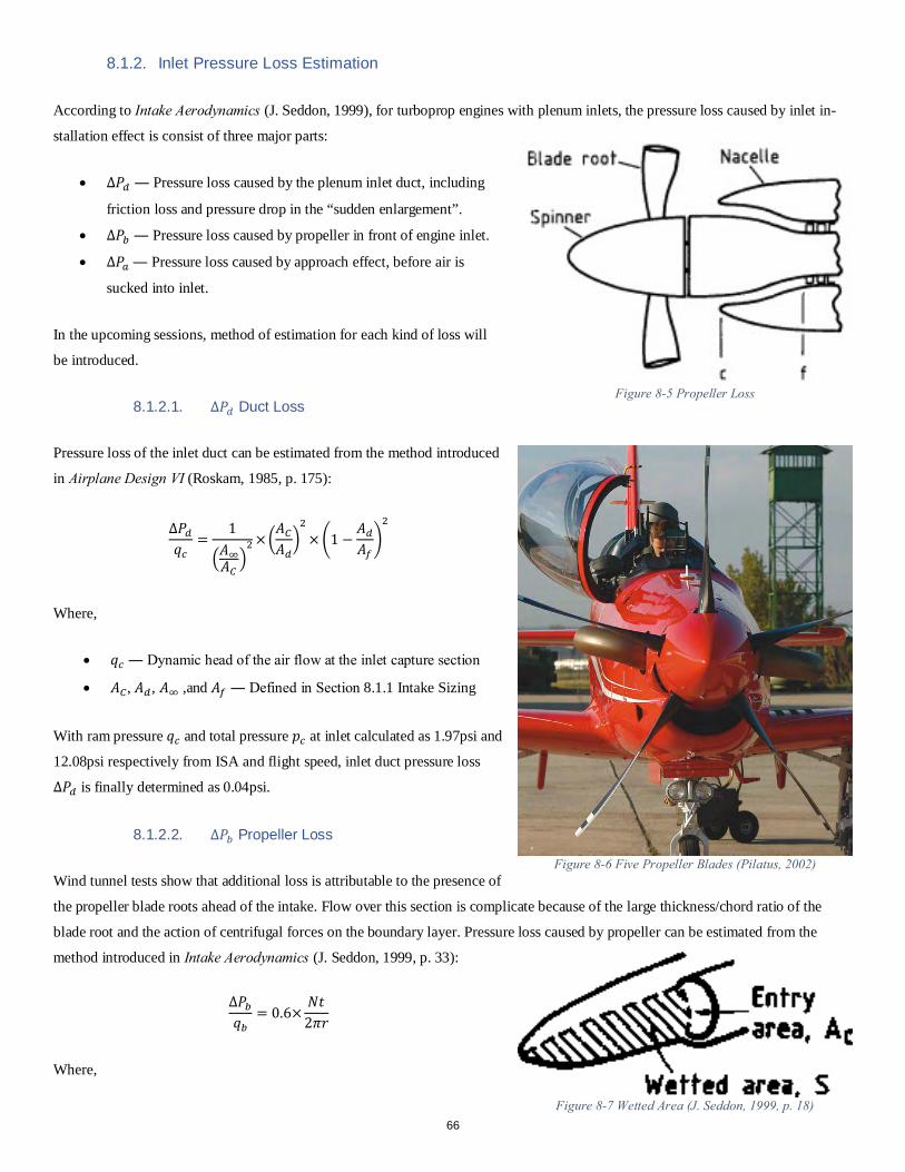
8.1.2. Inlet Pressure Loss Estimation
According to Intake Aerodynamics (J. Seddon, 1999), for turboprop engines with plenum inlets, the pressure loss caused by inlet in-
stallation effect is consist of three major parts:
• ∆𝑃𝑃𝑑𝑑 ― Pressure loss caused by the plenum inlet duct, including
friction loss and pressure drop in the “sudden enlargement”.
• ∆𝑃𝑃𝑙𝑙 ― Pressure loss caused by propeller in front of engine inlet.
• ∆𝑃𝑃𝐴𝐴 ― Pressure loss caused by approach effect, before air is
sucked into inlet.
In the upcoming sessions, method of estimation for each kind of loss will
be introduced.
8.1.2.1. ∆𝑃𝑃𝑑𝑑 Duct Loss
Pressure loss of the inlet duct can be estimated from the method introduced
in Airplane Design VI (Roskam, 1985, p. 175):
∆𝑃𝑃𝑑𝑑𝑞𝑞𝑉𝑉
=1
�𝐴𝐴∞𝐴𝐴𝑆𝑆�2 ×�
𝐴𝐴𝑆𝑆𝐴𝐴𝑑𝑑�2
× �1 −𝐴𝐴𝑑𝑑𝐴𝐴𝑟𝑟�2
Where,
• 𝑞𝑞𝑉𝑉 ― Dynamic head of the air flow at the inlet capture section
• 𝐴𝐴𝑆𝑆, 𝐴𝐴𝑑𝑑, 𝐴𝐴∞ ,and 𝐴𝐴𝑟𝑟 ― Defined in Section 8.1.1 Intake Sizing
With ram pressure 𝑞𝑞𝑉𝑉 and total pressure 𝑝𝑝𝑉𝑉 at inlet calculated as 1.97psi and
12.08psi respectively from ISA and flight speed, inlet duct pressure loss
∆𝑃𝑃𝑑𝑑 is finally determined as 0.04psi.
8.1.2.2. ∆𝑃𝑃𝑙𝑙 Propeller Loss
Wind tunnel tests show that additional loss is attributable to the presence of
the propeller blade roots ahead of the intake. Flow over this section is complicate because of the large thickness/chord ratio of the
blade root and the action of centrifugal forces on the boundary layer. Pressure loss caused by propeller can be estimated from the
method introduced in Intake Aerodynamics (J. Seddon, 1999, p. 33):
∆𝑃𝑃𝑙𝑙𝑞𝑞𝑙𝑙
= 0.6×𝑁𝑁𝑎𝑎
2𝜌𝜌𝑟𝑟
Where,
Figure 8-5 Propeller Loss
Figure 8-6 Five Propeller Blades (Pilatus, 2002)
Figure 8-7 Wetted Area (J. Seddon, 1999, p. 18) 66
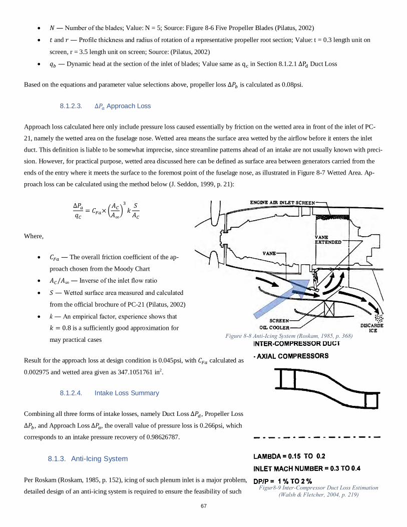
• 𝑁𝑁 ― Number of the blades; Value: N = 5; Source: Figure 8-6 Five Propeller Blades (Pilatus, 2002)
• 𝑎𝑎 and 𝑟𝑟 ― Profile thickness and radius of rotation of a representative propeller root section; Value: t = 0.3 length unit on
screen, r = 3.5 length unit on screen; Source: (Pilatus, 2002)
• 𝑞𝑞𝑙𝑙 ― Dynamic head at the section of the inlet of blades; Value same as qc in Section 8.1.2.1 ∆Pd Duct Loss
Based on the equations and parameter value selections above, propeller loss ∆𝑃𝑃𝑙𝑙 is calculated as 0.08psi.
8.1.2.3. ∆𝑃𝑃𝐴𝐴 Approach Loss
Approach loss calculated here only include pressure loss caused essentially by friction on the wetted area in front of the inlet of PC-
21, namely the wetted area on the fuselage nose. Wetted area means the surface area wetted by the airflow before it enters the inlet
duct. This definition is liable to be somewhat imprecise, since streamline patterns ahead of an intake are not usually known with preci-
sion. However, for practical purpose, wetted area discussed here can be defined as surface area between generators carried from the
ends of the entry where it meets the surface to the foremost point of the fuselage nose, as illustrated in Figure 8-7 Wetted Area. Ap-
proach loss can be calculated using the method below (J. Seddon, 1999, p. 21):
∆𝑃𝑃𝐴𝐴𝑞𝑞𝑆𝑆
= 𝐶𝐶𝑆𝑆𝐴𝐴× �𝐴𝐴𝑆𝑆𝐴𝐴∞
�3
𝑘𝑘𝑆𝑆𝐴𝐴𝑆𝑆
Where,
• 𝐶𝐶𝑆𝑆𝐴𝐴 ― The overall friction coefficient of the ap-
proach chosen from the Moody Chart
• 𝐴𝐴𝑆𝑆/𝐴𝐴∞ ― Inverse of the inlet flow ratio
• 𝑆𝑆 ― Wetted surface area measured and calculated
from the official brochure of PC-21 (Pilatus, 2002)
• k ― An empirical factor, experience shows that
𝑘𝑘 = 0.8 is a sufficiently good approximation for
may practical cases
Result for the approach loss at design condition is 0.045psi, with 𝐶𝐶𝑆𝑆𝐴𝐴 calculated as
0.002975 and wetted area given as 347.1051761 in2.
8.1.2.4. Intake Loss Summary
Combining all three forms of intake losses, namely Duct Loss ∆𝑃𝑃𝑑𝑑, Propeller Loss
∆𝑃𝑃𝑙𝑙, and Approach Loss ∆𝑃𝑃𝐴𝐴, the overall value of pressure loss is 0.266psi, which
corresponds to an intake pressure recovery of 0.98626787.
8.1.3. Anti-Icing System
Per Roskam (Roskam, 1985, p. 152), icing of such plenum inlet is a major problem,
detailed design of an anti-icing system is required to ensure the feasibility of such
Figure 8-8 Anti-Icing System (Roskam, 1985, p. 368)
Figur8-9 Inter-Compressor Duct Loss Estimation (Walsh & Fletcher, 2004, p. 219)
67
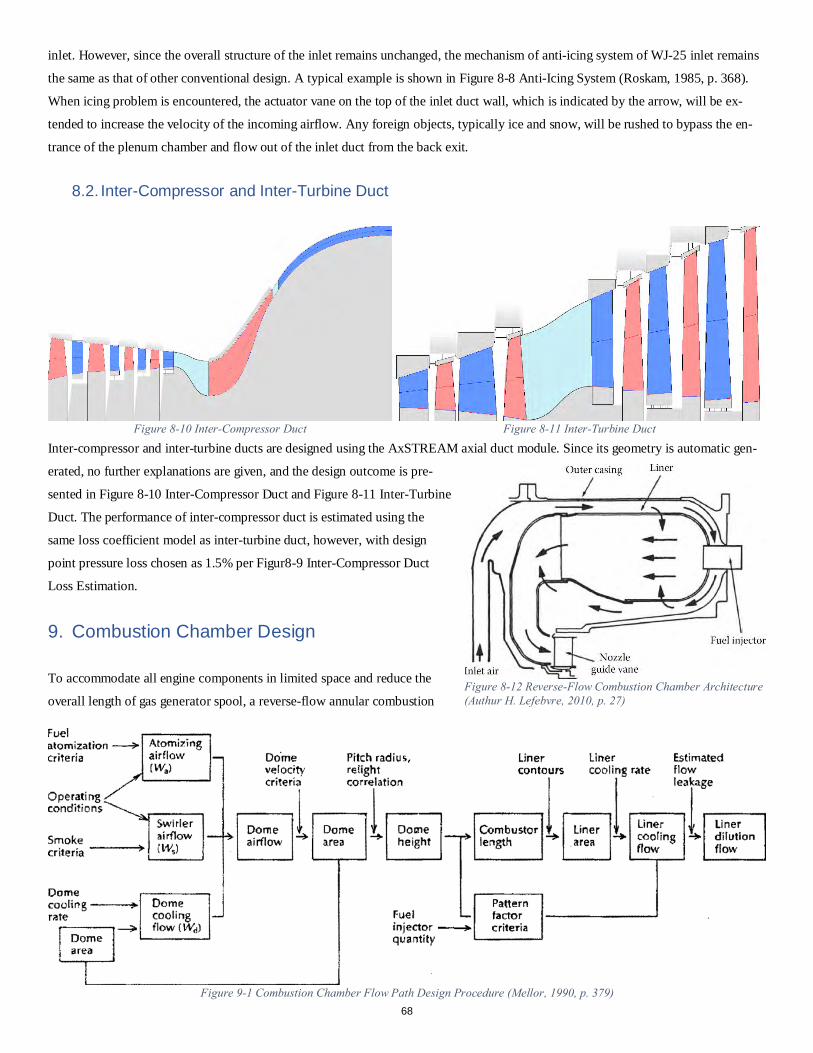
inlet. However, since the overall structure of the inlet remains unchanged, the mechanism of anti-icing system of WJ-25 inlet remains
the same as that of other conventional design. A typical example is shown in Figure 8-8 Anti-Icing System (Roskam, 1985, p. 368).
When icing problem is encountered, the actuator vane on the top of the inlet duct wall, which is indicated by the arrow, will be ex-
tended to increase the velocity of the incoming airflow. Any foreign objects, typically ice and snow, will be rushed to bypass the en-
trance of the plenum chamber and flow out of the inlet duct from the back exit.
8.2. Inter-Compressor and Inter-Turbine Duct
Inter-compressor and inter-turbine ducts are designed using the AxSTREAM axial duct module. Since its geometry is automatic gen-
erated, no further explanations are given, and the design outcome is pre-
sented in Figure 8-10 Inter-Compressor Duct and Figure 8-11 Inter-Turbine
Duct. The performance of inter-compressor duct is estimated using the
same loss coefficient model as inter-turbine duct, however, with design
point pressure loss chosen as 1.5% per Figur8-9 Inter-Compressor Duct
Loss Estimation.
9. Combustion Chamber Design
To accommodate all engine components in limited space and reduce the
overall length of gas generator spool, a reverse-flow annular combustion
Figure 8-10 Inter-Compressor Duct Figure 8-11 Inter-Turbine Duct
Figure 8-12 Reverse-Flow Combustion Chamber Architecture (Authur H. Lefebvre, 2010, p. 27)
Figure 9-1 Combustion Chamber Flow Path Design Procedure (Mellor, 1990, p. 379) 68
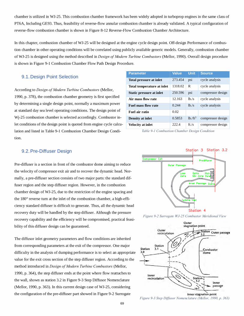
chamber is utilized in WJ-25. This combustion chamber framework has been widely adopted in turboprop engines in the same class of
PT6A, Including GE93. Thus, feasibility of reverse-flow annular combustion chamber is already validated. A typical configuration of
reverse-flow combustion chamber is shown in Figure 8-12 Reverse-Flow Combustion Chamber Architecture.
In this chapter, combustion chamber of WJ-25 will be designed at the engine cycle design point. Off-design Performance of combus-
tion chamber in other operating conditions will be correlated using publicly available generic models. Generally, combustion chamber
of WJ-25 is designed using the method described in Design of Modern Turbine Combustors (Mellor, 1990). Overall design procedure
is shown in Figure 9-1 Combustion Chamber Flow Path Design Procedure.
9.1. Design Point Selection
According to Design of Modern Turbine Combustors (Mellor,
1990, p. 378), the combustion chamber geometry is first specified
by determining a single design point, normally a maximum power
at standard day sea level operating conditions. The design point of
Wj-25 combustion chamber is selected accordingly. Combustor in-
let conditions of the design point is quoted from engine cycle calcu-
lation and listed in Table 9-1 Combustion Chamber Design Condi-
tion.
9.2. Pre-Diffuser Design
Pre-diffuser is a section in front of the combustor dome aiming to reduce
the velocity of compressor exit air and to recover the dynamic head. Nor-
mally, a pre-diffuser section consists of two major parts: the standard dif-
fuser region and the step diffuser region. However, in the combustion
chamber design of WJ-25, due to the restriction of the engine spacing and
the 180° reverse turn at the inlet of the combustion chamber, a high-effi-
ciency standard diffuser is difficult to generate. Thus, all the dynamic head
recovery duty will be handled by the step diffuser. Although the pressure
recovery capability and the efficiency will be compromised, practical feasi-
bility of this diffuser design can be guaranteed.
The diffusor inlet geometry parameters and flow conditions are inherited
from corresponding parameters at the exit of the compressor. One major
difficulty in the analysis of dumping performance is to select an appropriate
value for the exit cross section of the step diffuser region. According to the
method introduced in Design of Modern Turbine Combustors (Mellor,
1990, p. 364), the step diffuser ends at the point where flow reattaches to
the wall, shown as station 3.2 in Figure 9-3 Step Diffusor Nomenclature
(Mellor, 1990, p. 363). In this current design case of WJ-25, considering
the configuration of the pre-diffuser part showed in Figure 9-2 Surrogate
Parameter Value Unit Source
Total pressure at inlet 273.454 psi cycle analysis
Total temperature at inlet 1318.02 R cycle analysis
Static pressure at inlet 250.596 psi compressor design
Air mass flow rate 12.163 lb./s cycle analysis
Fuel mass flow rate 0.244 lb./s cycle analysis
Fuel air ratio 0.02
Density at inlet 0.5853 lb./ft3 compressor design
Velocity at inlet 222.4 ft./s compressor design
Table 9-1 Combustion Chamber Design Condition
Figure 9-2 Surrogate WJ-25 Combustor Meridional View
Figure 9-3 Step Diffusor Nomenclature (Mellor, 1990, p. 363) 69
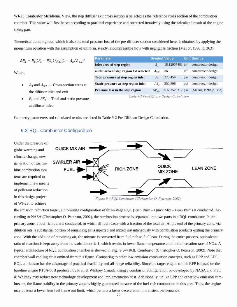
WJ-25 Combustor Meridional View, the step diffuser exit cross section is selected as the reference cross section of the combustion
chamber. This value will first be set according to practical experience and corrected iteratively using the calculated result of the engine
sizing part.
Theoretical dumping loss, which is also the total pressure loss of the pre-diffuser section considered here, is obtained by applying the
momentum equation with the assumption of uniform, steady, incompressible flow with negligible friction (Mellor, 1990, p. 363):
∆𝑃𝑃𝑑𝑑 = 𝑃𝑃3[(𝑃𝑃3 −𝑃𝑃𝑆𝑆3) 𝑝𝑝3⁄ ][1 − 𝐴𝐴3 𝐴𝐴3.2⁄ ]2
Where,
• 𝐴𝐴3 and 𝐴𝐴3.2 ― Cross-section areas at
the diffuser inlet and exit
• 𝑃𝑃3 and 𝑃𝑃𝑆𝑆3― Total and static pressure
at diffuser inlet
Geometry parameters and calculated results are listed in Table 9-2 Pre-Diffusor Design Calculation.
9.3. RQL Combustor Configuration
Under the pressure of
globe warming and
climate change, new
generation of gas tur-
bine combustion sys-
tems are required to
implement new means
of pollutant reduction.
In this design project
of WJ-25, to achieve
the emission reduction target, a promising configuration of three-stage RQL (Rich Burn – Quick Mix – Lean Burn) is conducted. Ac-
cording to NASA (Christopher O. Peterson, 2002), the combustion process is separated into two parts in a RQL combustor. In the
primary zone, a fuel-rich burn is conducted, in which all fuel reacts with a fraction of the total air. At the end of the primary zone, via
dilution jets, a substantial portion of remaining air is injected and mixed instantaneously with combustion products exiting the primary
zone. With the addition of remaining air, the mixture is converted from fuel rich to fuel lean. During the entire process, equivalence
ratio of reaction is kept away from the stoichiometric 1, which results in lower flame temperature and limited creation rate of NOx. A
typical architecture of RQL combustion chamber is showed in Figure 9-4 RQL Combustor (Christopher O. Peterson, 2002). Note that
chamber wall cooling air is omitted from this figure. Comparing to other low emission combustion concepts, such as LPP and LDI,
RQL combustor has the advantage of practical feasibility and all-range reliability. Since the target engine of this RFP is based on the
baseline engine PT6A-68B produced by Pratt & Whitney Canada, using a combustor configuration co-developed by NASA and Pratt
& Whitney may reduce new technology development and implementation cost. Additionally, unlike LPP and other low emission com-
bustors, the flame stability in the primary zone is highly guaranteed because of the fuel-rich combustion in this area. Thus, the engine
may possess a lower lean fuel flame out limit, which permits a faster deceleration in transient performance.
Parameter Symbol Value Unit Source
Inlet area of step region 𝐴𝐴3 18.12957481 in2 compressor design
outlet area of step region 1st selected 𝐴𝐴3 .2 36 in2 compressor design
Total pressure at step region inlet 𝑃𝑃3 273.454 psi compressor design
Static pressure at step region inlet 𝑃𝑃𝑆𝑆3 250.596 psi compressor design
Pressure loss in the step region ∆𝑃𝑃𝑑𝑑𝑐𝑐𝐴𝐴 5.632523317 psi (Mellor, 1990, p. 363)
Table 9-2 Pre-Diffusor Design Calculation
Figure 9-4 RQL Combustor (Christopher O. Peterson, 2002)
70
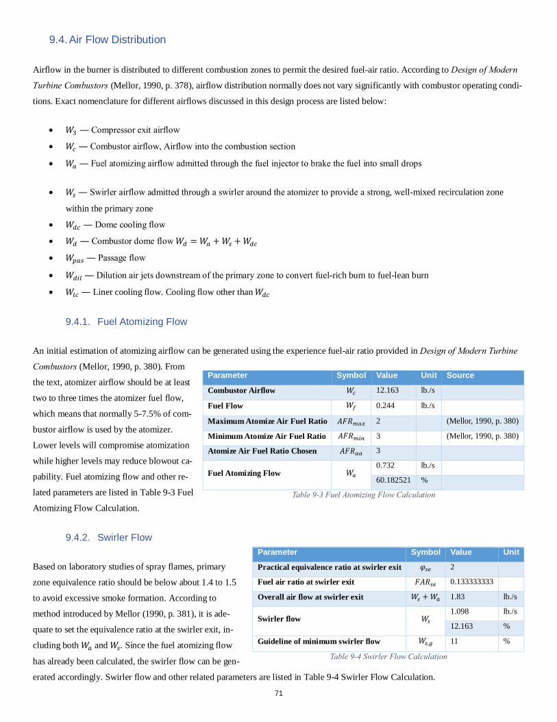
9.4. Air Flow Distribution
Airflow in the burner is distributed to different combustion zones to permit the desired fuel-air ratio. According to Design of Modern
Turbine Combustors (Mellor, 1990, p. 378), airflow distribution normally does not vary significantly with combustor operating condi-
tions. Exact nomenclature for different airflows discussed in this design process are listed below:
• 𝑘𝑘3 ― Compressor exit airflow
• 𝑘𝑘𝑉𝑉 ― Combustor airflow, Airflow into the combustion section
• 𝑘𝑘𝐴𝐴 ― Fuel atomizing airflow admitted through the fuel injector to brake the fuel into small drops
• 𝑘𝑘𝑐𝑐 ― Swirler airflow admitted through a swirler around the atomizer to provide a strong, well-mixed recirculation zone
within the primary zone
• 𝑘𝑘𝑑𝑑𝑉𝑉 ― Dome cooling flow
• 𝑘𝑘𝑑𝑑 ― Combustor dome flow 𝑘𝑘𝑑𝑑 = 𝑘𝑘𝐴𝐴 + 𝑘𝑘𝑐𝑐 + 𝑘𝑘𝑑𝑑𝑉𝑉
• 𝑘𝑘𝑖𝑖𝐴𝐴𝑐𝑐 ― Passage flow
• 𝑘𝑘𝑑𝑑𝐸𝐸𝐴𝐴 ― Dilution air jets downstream of the primary zone to convert fuel-rich burn to fuel-lean burn
• 𝑘𝑘𝐴𝐴𝑉𝑉 ― Liner cooling flow. Cooling flow other than 𝑘𝑘𝑑𝑑𝑉𝑉
9.4.1. Fuel Atomizing Flow
An initial estimation of atomizing airflow can be generated using the experience fuel-air ratio provided in Design of Modern Turbine
Combustors (Mellor, 1990, p. 380). From
the text, atomizer airflow should be at least
two to three times the atomizer fuel flow,
which means that normally 5-7.5% of com-
bustor airflow is used by the atomizer.
Lower levels will compromise atomization
while higher levels may reduce blowout ca-
pability. Fuel atomizing flow and other re-
lated parameters are listed in Table 9-3 Fuel
Atomizing Flow Calculation.
9.4.2. Swirler Flow
Based on laboratory studies of spray flames, primary
zone equivalence ratio should be below about 1.4 to 1.5
to avoid excessive smoke formation. According to
method introduced by Mellor (1990, p. 381), it is ade-
quate to set the equivalence ratio at the swirler exit, in-
cluding both 𝑘𝑘𝐴𝐴 and 𝑘𝑘𝑐𝑐. Since the fuel atomizing flow
has already been calculated, the swirler flow can be gen-
erated accordingly. Swirler flow and other related parameters are listed in Table 9-4 Swirler Flow Calculation.
Parameter Symbol Value Unit Source
Combustor Airflow 𝑘𝑘𝑉𝑉 12.163 lb./s
Fuel Flow 𝑘𝑘𝑟𝑟 0.244 lb./s
Maximum Atomize Air Fuel Ratio 𝐴𝐴𝐹𝐹𝑅𝑅𝑖𝑖𝐴𝐴𝐸𝐸 2 (Mellor, 1990, p. 380)
Minimum Atomize Air Fuel Ratio 𝐴𝐴𝐹𝐹𝑅𝑅𝑖𝑖𝐸𝐸𝑖𝑖 3 (Mellor, 1990, p. 380)
Atomize Air Fuel Ratio Chosen 𝐴𝐴𝐹𝐹𝑅𝑅𝐴𝐴𝐴𝐴 3
Fuel Atomizing Flow 𝑘𝑘𝐴𝐴 0.732 lb./s
60.182521 %
Table 9-3 Fuel Atomizing Flow Calculation
Parameter Symbol Value Unit
Practical equivalence ratio at swirler exit 𝜑𝜑𝑐𝑐𝑉𝑉 2
Fuel air ratio at swirler exit 𝐹𝐹𝐴𝐴𝑅𝑅𝑐𝑐𝑉𝑉 0.133333333
Overall air flow at swirler exit 𝑘𝑘𝑐𝑐 + 𝑘𝑘𝐴𝐴 1.83 lb./s
Swirler flow 𝑘𝑘𝑐𝑐 1.098 lb./s
12.163 %
Guideline of minimum swirler flow 𝑘𝑘𝑐𝑐,𝐴𝐴 11 %
Table 9-4 Swirler Flow Calculation
71
9.4.3. Dome Cooling Flow
Estimation of the dome cooling flow needs to be
based on the total area to be cooled. However, at this
point, a dome cooling flow can be estimated accord-
ing to previous experience to carry on the combustor
sizing process. An accurate value will be updated after
actual dome area has been calculated. Dome cooling
flow and other related parameters are listed in Table
9-5 Dome Cooling Flow.
9.4.4. Passage Air Flow, Dilution Flow and Liner Cooling Flow
According to Mellor (1990, p. 389), normally in a RQL com-
bustor, the equivalence ratio in the secondary zone should be
between 0.5 and 0.8. Higher levels will increase NOx emis-
sion, while lower levels may result in quench, when engine is
working at sever part load conditions. Passage air flow, dilu-
tion flow, liner cooling flow and related parameters are listed
in Table 9-6 Passage Air Flow, Dilution Flow and Liner
Cooling Flow.
9.5. Combustion Chamber Sizing 9.5.1. Reference Area Calculation
Reference areas are calculated using “velocity method” introduced by Mellor (1990, p. 383). According to this method, dome and
passage reference velocities are chosen from previous design. In this design project, to simplify the calculation, passage airflow is
assumed to be split equally between inner and outer passages. Once reference velocities are selected, dome and passage areas can be
easily calculated using equation:
𝐴𝐴𝐸𝐸 = 𝑘𝑘𝐸𝐸/(𝜌𝜌3𝑉𝑉𝐸𝐸)
Where,
• 𝐴𝐴𝐸𝐸, 𝑘𝑘𝐸𝐸 and 𝑉𝑉𝐸𝐸 ― Area, airflow
and velocity of a section
• 𝜌𝜌3 ― Air density at the com-
bustion chamber inlet
Reference areas and other parameters calculated are listed in Table 9-7 Reference Area Calculation.
Parameter Symbol Value Unit
Experimental dome cooling rate 𝐶𝐶𝑅𝑅𝑑𝑑 0.5 kg (s×m2×atm)⁄
4.83921E-05 lb./(s×in2×psi)
Dome cooling flow rate assumed 0.15
Dome cooling flow assumed 𝑘𝑘𝑑𝑑𝑉𝑉,𝐴𝐴 1.82445 lb./s
Dome air flow 𝑘𝑘𝑑𝑑 3.65445 lb./s
30.0456302 %
Table 9-5 Dome Cooling Flow
Parameter Symbol Value Unit
Passage air flow 𝑘𝑘𝑖𝑖 8.50855 lb./s
69.95436981 %
Equivalence ratio selected 𝜑𝜑𝑖𝑖 0.5
Dilution flow at the primary zone exit 𝑘𝑘𝑑𝑑𝐸𝐸𝐴𝐴 7.176470588 lb./s
59.00247133 %
Liner cooling flow 𝑘𝑘𝐴𝐴𝑉𝑉 1.332079412 lb./s
10.9518985 %
Table 9-6 Passage Air Flow, Dilution Flow and Liner Cooling Flow
Parameter Symbol Value Unit
Dome reference velocity selected 𝑉𝑉𝐴𝐴𝑑𝑑𝑉𝑉𝑖𝑖 32.80839895 ft/s
Passage reference velocity selected 𝑉𝑉𝐴𝐴𝑖𝑖𝐴𝐴𝑐𝑐 164.0419948 ft/s
Dome reference area 𝐴𝐴𝐴𝐴𝑑𝑑𝑉𝑉𝑖𝑖0.190308621 ft2
27.40444146 in2
Passage reference area 𝐴𝐴𝐴𝐴𝑑𝑑𝑉𝑉𝑖𝑖0.088618009 ft2
12.76099333 in2
Reference area 𝐴𝐴𝐴𝐴𝑉𝑉𝑟𝑟 40.16543478 in2
Table 9-7 Reference Area Calculation
72
9.5.2. Dome and Passage Height
After dome and passage areas are specified, dome and pas-
sage height can be calculated using the method introduced
by Mellor (1990, p. 386):
𝑆𝑆𝐷𝐷 = 𝐴𝐴𝐴𝐴𝑉𝑉𝑟𝑟/(𝜌𝜌𝐷𝐷𝑖𝑖𝑉𝑉𝐴𝐴𝑖𝑖)
Where,
• 𝑆𝑆𝐷𝐷 ― Height of the dome
• 𝐴𝐴𝐴𝐴𝑉𝑉𝑟𝑟 ― Reference area of the combustion chamber
• 𝐷𝐷𝑖𝑖𝑉𝑉𝐴𝐴𝑖𝑖 ― Mean diameter of the combustor
Calculated results and other parameters are listed in Table 9-8
Dome and Passage Height Calculation.
9.5.3. Number of Fuel Injectors and Length of Combustor
According to Mellor (1990, p. 387), the number of fuel injectors should be selected such that injector spacing 𝐵𝐵 is about the same as
the combustor dome height. Number of fuel injectors, length of the chamber and other related parameters are listed in Table 9-9 Fuel
Injector Number & Burner Length.
9.5.4. 3D Geometry of Combustion Chamber
After all the above-mentioned calculations, the geometrical parame-
ters are integrated together in a single 3D model of the combustion
chamber. Noting that the purpose of this 3D model is demonstrative
for the afore calculated areas, length, numbers, etc., its geometry is
only representative instead of exact. A picture of the model is pre-
sented in Figure 9-6 3D Combustion Chamber Model
10. Engine Component Test
To facilitate off-design calculation, the component off-design data, such as compressor and turbine map, need to be calculated. In this
section, four component types are tested numerically, including compressor, turbine, inlet, and burner.
10.1. Compressor Test
Testbed compressor rig test is usually done with atmospheric inlet condition while outlet being throttled. Thus, the numerical test also
follows this legacy. With total temperature and pressure at inlet fixed as ISA SLS values, outlet pressure and mechanical spool speed
are chosen as variable. Target values include total-to-total efficiency, inlet corrected mass flow rate, pressure ratio, and corrected spool
Parameter Symbol Value Unit
Combustor tip diameter selected 𝐷𝐷𝐸𝐸𝑉𝑉𝑉𝑉𝑖𝑖𝑙𝑙 15.5 in
Combustor hub diameter 1st calculated 𝐷𝐷ℎ𝑉𝑉𝑉𝑉𝑖𝑖𝑙𝑙 11.42270337 in
Combustor mean diameter selected 𝐷𝐷𝑖𝑖𝑉𝑉𝑉𝑉𝑖𝑖𝑙𝑙 13 in
Combustor height calculated 𝑆𝑆𝑉𝑉 1.96 in
Dome height calculated 𝑆𝑆𝑑𝑑 1.1 in
Half passage height 𝑆𝑆𝑖𝑖 0.43 in
Table 9-8 Dome and Passage Height Calculation
Parameter Symbol Value Unit
Injector spacing 𝐵𝐵 1.1 in
Mean perimeter of combustor 𝐶𝐶𝑖𝑖 40.8407 in
Number of fuel injectors calculated 𝑁𝑁𝑟𝑟𝐸𝐸,𝑉𝑉 37.12791
Number of fuel injectors selected 𝑁𝑁𝑟𝑟𝐸𝐸 20
Combustor length to height ratio 𝐿𝐿𝑉𝑉/𝑆𝑆𝑑𝑑 4
Combustor length 𝐿𝐿𝑉𝑉 4.4 in
Table 9-9 Fuel Injector Number & Burner Length
Figure 9-5 3D Combustion Chamber Model
73
speed. Results for both axial and centrifugal compressors are presented in Figure 10-1 Axial Compressor Map and Figure 10-2 Centri-
fugal Compressor Map. Noting that maps shown here have been maunally smoothed to attain a more reasonable illustration.
Special note need to be given for axial compressor since a VSV schedule is incorporated with this map test. VSV is well-known for its
capability of improving the part load performance. Since it regulates the stagger angle of certain stages of stator vanes, it helps the
metal geometry to refit with the varied airflow angle. Therefore, the angle of incidence on the blade cascade is also minimized, which
in turn avoids surge and improves efficiency. The only non-satisfying characteristic of VSV is its effect of reducing mass flow rate
when flow passage becomes narrow during the re-staggering. However, this fact doesn’t manage to limit its popularity in modern
compressors, even in advanced turboprop engines, such as GE93. Thus, the axial compressor of WJ-25 also facilitates a 1st stage varia-
ble vane, while the staggering schedule of this stage of stator is also tested numerically. For the testing of staggering schedule, SoftIn-
Way provided the user with a lengthy and complicated operation tutorial. Physical principle of the numerical test resembles that of the
real rig test for VSV schedule. Namely, the operating points on each corrected speed line should firstly be determined. Then the stag-
ger angle is optimized for each operating point on each spool speed line. However, if this procedure is
strictly followed, then the off design steady state co-working line must be first calculated. Therefore, a sim-
plification is adopted: due to fact that off design co-working line of a gas turbine engine compressor nor-
mally lies within the vicinity of the point of peak efficiency on each corrected spool speed line, the VSV is
in fact optimized for the point of peak efficiency instead of off-design working point. A tabular demonstra-
tion of the final VSV schedule is presented in Table 10-1 VSV Schedule.
10.2. Turbine Test
Similar as compressor test, the numerical turbine test also
follows the legacy of rig test. Namely, the outlet condition is
set as atmospheric while the inlet pressure is being varied.
With total pressure at outlet fixed as ISA SLS values, inlet
pressure and mechanical spool speed are chosen as variable.
Target values include total-to-total efficiency, inlet corrected
mass flow rate, pressure ratio, and corrected spool speed. Re-
sults for both GGT and FPT are presented in Figure 10-4
GGT Map and Figure 10-5 FPT Map respectively.
RPM RA
44000 -2
39600 0
33000 1.5
28600 4.5
22000 6.5
Table 10-1 VSV Schedule
0.9750
0.9800
0.9850
0.9900
0.9950
1.0000
Pres
sure
Rec
over
y
Corrected Mass Flow Rate (lb/s)
0.560.5
Figure 10-3 Intake Map
Figure 10-1 Axial Compressor Map Figure 10-2 Centrifugal Compressor Map
74
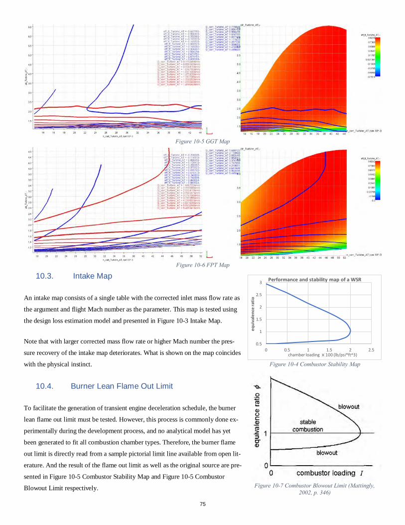
10.3. Intake Map
An intake map consists of a single table with the corrected inlet mass flow rate as
the argument and flight Mach number as the parameter. This map is tested using
the design loss estimation model and presented in Figure 10-3 Intake Map.
Note that with larger corrected mass flow rate or higher Mach number the pres-
sure recovery of the intake map deteriorates. What is shown on the map coincides
with the physical instinct.
10.4. Burner Lean Flame Out Limit
To facilitate the generation of transient engine deceleration schedule, the burner
lean flame out limit must be tested. However, this process is commonly done ex-
perimentally during the development process, and no analytical model has yet
been generated to fit all combustion chamber types. Therefore, the burner flame
out limit is directly read from a sample pictorial limit line available from open lit-
erature. And the result of the flame out limit as well as the original source are pre-
sented in Figure 10-5 Combustor Stability Map and Figure 10-5 Combustor
Blowout Limit respectively.
Figure 10-5 GGT Map
Figure 10-6 FPT Map
Figure 10-7 Combustor Blowout Limit (Mattingly, 2002, p. 346)
Figure 10-4 Combustor Stability Map
0.5
1
1.5
2
2.5
3
0 0.5 1 1.5 2 2.5
equi
vale
nce
ratio
chamber loading ⅹ100 (lb/psi*ft^3)
Performance and stability map of a WSR
75
11. Off-Design and Transient Performance
To design the engine controllers with more flexibility and present the off-design and transient performance with higher precision, an
open source gas turbine modeling code T-MATS (NASA Glenn Research Center, 2014) from NASA has been utilized as platform for
achieving this purpose. However, extensive amount of correction algorithms and modifications have been added to improve the level
of fidelity.
11.1. Steady-State Model Building and Verifications
In this section, the modeling process for the steady state is demonstrated. Basic architecture of the model is the same as Figure 4-2 0-D
Engine Model, however, with the axial and centrifugal compressor modeled separately as shown in Figure 4-1 Axial-Centrifugal
Compressor. Some of the imbedded component model blocks in T-MATS have been modified to obtain a higher compatibility with
the model from GasTurb, which will be demonstrated in greater details later in this section.
11.1.1. Steady-State Model Overview
An overview of the steady state MATLAB model is presented in Figure 11-1 Steady-State Model Overview.
11.1.2. Main Corrections and Modifications
This section presents correction algorithms proprietary to off design calculations. Design condition model correction are included,
however, not mentioned again here.
Figure 11-1 Steady-State Model Overview
76
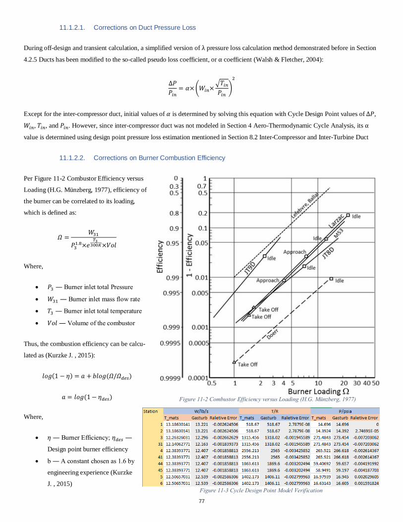
11.1.2.1. Corrections on Duct Pressure Loss
During off-design and transient calculation, a simplified version of λ pressure loss calculation method demonstrated before in Section
4.2.5 Ducts has been modified to the so-called pseudo loss coefficient, or α coefficient (Walsh & Fletcher, 2004):
∆𝑃𝑃𝑃𝑃𝐸𝐸𝑖𝑖
= 𝛼𝛼×�𝑘𝑘𝐸𝐸𝑖𝑖×�𝑂𝑂𝐸𝐸𝑖𝑖𝑃𝑃𝐸𝐸𝑖𝑖
�2
Except for the inter-compressor duct, initial values of 𝛼𝛼 is determined by solving this equation with Cycle Design Point values of ∆𝑃𝑃,
𝑘𝑘𝐸𝐸𝑖𝑖, 𝑂𝑂𝐸𝐸𝑖𝑖, and 𝑃𝑃𝐸𝐸𝑖𝑖. However, since inter-compressor duct was not modeled in Section 4 Aero-Thermodynamic Cycle Analysis, its α
value is determined using design point pressure loss estimation mentioned in Section 8.2 Inter-Compressor and Inter-Turbine Duct
11.1.2.2. Corrections on Burner Combustion Efficiency
Per Figure 11-2 Combustor Efficiency versus
Loading (H.G. Münzberg, 1977), efficiency of
the burner can be correlated to its loading,
which is defined as:
𝛺𝛺 =𝑘𝑘31
𝑃𝑃31.8×𝑠𝑠𝑇𝑇3 300𝐾𝐾×𝑉𝑉𝑠𝑠𝑙𝑙
Where,
• 𝑃𝑃3 ― Burner inlet total Pressure
• 𝑘𝑘31 ― Burner inlet mass flow rate
• 𝑂𝑂3 ― Burner inlet total temperature
• 𝑉𝑉𝑠𝑠𝑙𝑙 ― Volume of the combustor
Thus, the combustion efficiency can be calcu-
lated as (Kurzke J. , 2015):
𝑙𝑙𝑠𝑠𝑘𝑘(1 − 𝜂𝜂) = 𝑎𝑎 + 𝑙𝑙𝑙𝑙𝑠𝑠𝑘𝑘(𝛺𝛺/𝛺𝛺𝑑𝑑𝑉𝑉𝑐𝑐)
𝑎𝑎 = 𝑙𝑙𝑠𝑠𝑘𝑘 (1− 𝜂𝜂𝑑𝑑𝑉𝑉𝑐𝑐)
Where,
• 𝜂𝜂 ― Burner Efficiency; 𝜂𝜂𝑑𝑑𝑉𝑉𝑐𝑐 ―
Design point burner efficiency
• b ― A constant chosen as 1.6 by
engineering experience (Kurzke
J. , 2015)
Figure 11-2 Combustor Efficiency versus Loading (H.G. Münzberg, 1977)
77
Figure 11-3 Cycle Design Point Model Verification
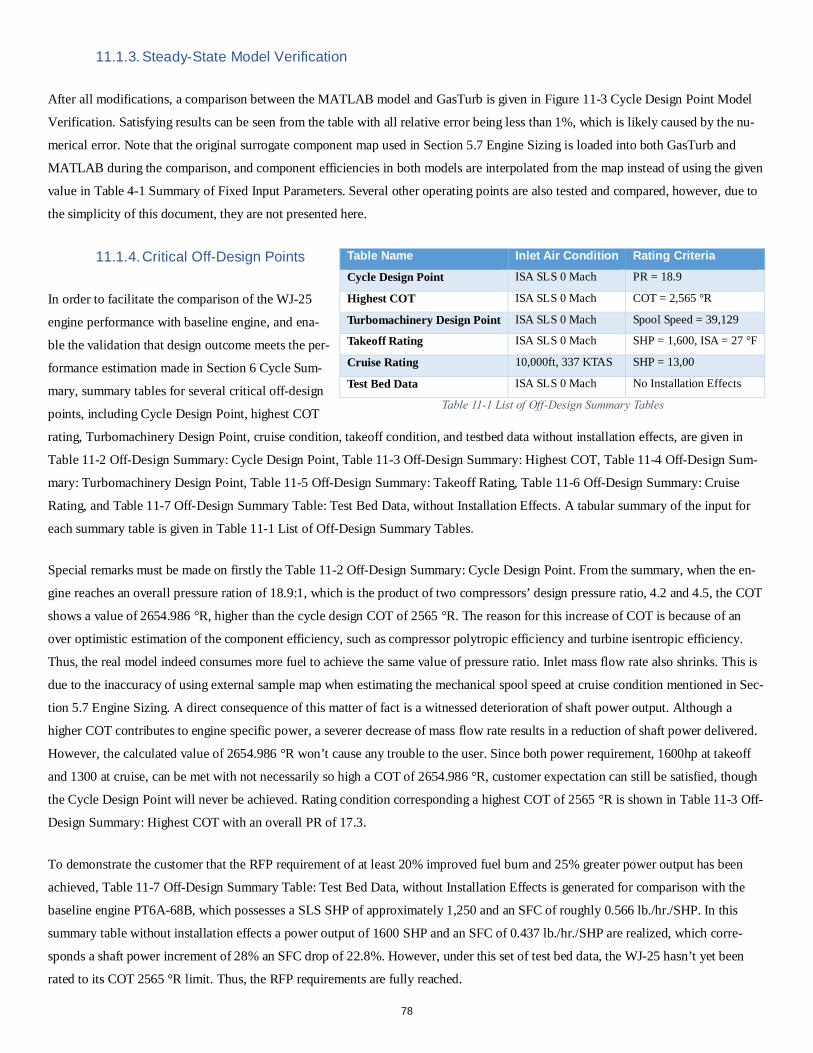
11.1.3. Steady-State Model Verification
After all modifications, a comparison between the MATLAB model and GasTurb is given in Figure 11-3 Cycle Design Point Model
Verification. Satisfying results can be seen from the table with all relative error being less than 1%, which is likely caused by the nu-
merical error. Note that the original surrogate component map used in Section 5.7 Engine Sizing is loaded into both GasTurb and
MATLAB during the comparison, and component efficiencies in both models are interpolated from the map instead of using the given
value in Table 4-1 Summary of Fixed Input Parameters. Several other operating points are also tested and compared, however, due to
the simplicity of this document, they are not presented here.
11.1.4. Critical Off-Design Points
In order to facilitate the comparison of the WJ-25
engine performance with baseline engine, and ena-
ble the validation that design outcome meets the per-
formance estimation made in Section 6 Cycle Sum-
mary, summary tables for several critical off-design
points, including Cycle Design Point, highest COT
rating, Turbomachinery Design Point, cruise condition, takeoff condition, and testbed data without installation effects, are given in
Table 11-2 Off-Design Summary: Cycle Design Point, Table 11-3 Off-Design Summary: Highest COT, Table 11-4 Off-Design Sum-
mary: Turbomachinery Design Point, Table 11-5 Off-Design Summary: Takeoff Rating, Table 11-6 Off-Design Summary: Cruise
Rating, and Table 11-7 Off-Design Summary Table: Test Bed Data, without Installation Effects. A tabular summary of the input for
each summary table is given in Table 11-1 List of Off-Design Summary Tables.
Special remarks must be made on firstly the Table 11-2 Off-Design Summary: Cycle Design Point. From the summary, when the en-
gine reaches an overall pressure ration of 18.9:1, which is the product of two compressors’ design pressure ratio, 4.2 and 4.5, the COT
shows a value of 2654.986 °R, higher than the cycle design COT of 2565 °R. The reason for this increase of COT is because of an
over optimistic estimation of the component efficiency, such as compressor polytropic efficiency and turbine isentropic efficiency.
Thus, the real model indeed consumes more fuel to achieve the same value of pressure ratio. Inlet mass flow rate also shrinks. This is
due to the inaccuracy of using external sample map when estimating the mechanical spool speed at cruise condition mentioned in Sec-
tion 5.7 Engine Sizing. A direct consequence of this matter of fact is a witnessed deterioration of shaft power output. Although a
higher COT contributes to engine specific power, a severer decrease of mass flow rate results in a reduction of shaft power delivered.
However, the calculated value of 2654.986 °R won’t cause any trouble to the user. Since both power requirement, 1600hp at takeoff
and 1300 at cruise, can be met with not necessarily so high a COT of 2654.986 °R, customer expectation can still be satisfied, though
the Cycle Design Point will never be achieved. Rating condition corresponding a highest COT of 2565 °R is shown in Table 11-3 Off-
Design Summary: Highest COT with an overall PR of 17.3.
To demonstrate the customer that the RFP requirement of at least 20% improved fuel burn and 25% greater power output has been
achieved, Table 11-7 Off-Design Summary Table: Test Bed Data, without Installation Effects is generated for comparison with the
baseline engine PT6A-68B, which possesses a SLS SHP of approximately 1,250 and an SFC of roughly 0.566 lb./hr./SHP. In this
summary table without installation effects a power output of 1600 SHP and an SFC of 0.437 lb./hr./SHP are realized, which corre-
sponds a shaft power increment of 28% an SFC drop of 22.8%. However, under this set of test bed data, the WJ-25 hasn’t yet been
rated to its COT 2565 °R limit. Thus, the RFP requirements are fully reached.
Table Name Inlet Air Condition Rating Criteria
Cycle Design Point ISA SLS 0 Mach PR = 18.9
Highest COT ISA SLS 0 Mach COT = 2,565 °R
Turbomachinery Design Point ISA SLS 0 Mach Spool Speed = 39,129
Takeoff Rating ISA SLS 0 Mach SHP = 1,600, ISA = 27 °F
Cruise Rating 10,000ft, 337 KTAS SHP = 13,00
Test Bed Data ISA SLS 0 Mach No Installation Effects
Table 11-1 List of Off-Design Summary Tables
78
Table 11-2 Off-Design Summary: Cycle Design Point
Table 11-3 Off-Design Summary: Highest COT
Table 11-4 Off-Design Summary: Turbomachinery Design Point
Cycle Design Point(PR=18.9)===SUMMARY OUTPUT DATA===MN alt dTamb VTAS N1 N2 T41 SHP THP ESHP BSFC ESFC0 0 0 0 41093.59326 21041 2654.986132 2087.642072 0 2087.642072 0.449675766 0.449675766
===FLOW STATION DATA===W/lb/s ht Tt/R Pt/psi FAR Pi Wc Ps Ts R gamt Aera Ma
1 Inlet 12.98697638 123.954269 518.6700145 14.696 0 0.022059391 12.98697656 14.696 518.6700145 0.06856 1.4 50.5 02 AC_in 12.98697638 123.954269 518.6700145 14.37181519 0 5.129127673 13.27992358 10.38679549 472.712235 0.06856 1.4 38.35870022 0.69721424 AC_out 12.07788803 212.0074372 882.629012 73.71487502 0 0.013560672 3.141076717 61.96089393 839.8943098 0.06856 1.4 15.286917 0.50438625 CC_in 12.07788803 212.0074372 882.629012 72.71525179 0 3.735492905 3.184257386 68.49369461 867.6744179 0.06856 1.4 20.24192531 0.2935583 CC_out 11.95710915 321.2377785 1316.576772 271.6273071 0 0.020929909 1.030693266 265.8643434 1308.534678 0.06856 1.4 25.55443075 0.1752984 GGT_in 12.21787639 710.1925395 2654.986132 265.9421723 0.021808552 4.20280221 1.527542219 256.6613452 2638.286649 0.06861 1.216 11.52079622 0.24209144 GGT_out 12.21787639 508.5553453 1969.531444 63.27734662 0.021808552 0.00992727 5.529457256 59.56259562 1948.478923 0.06861 1.216 35.49304337 0.31629545 FPT_in 12.21787639 508.5553453 1969.531444 62.64917529 0.021808552 3.627519444 5.58490007 60.3331162 1956.39677 0.06861 1.216 41.78869454 0.2493275 FPT_out 12.21787639 387.7881463 1539.311343 17.27052777 0.021808552 0.0185834 17.91046788 15.86874758 1516.338659 0.06861 1.216 92.50119511 0.3745386 Nozzle_in 12.33865527 387.7881463 1537.131071 16.94958264 0.02113417 1.153346669 18.41695602 16.55463064 1531.586727 0.06861 1.181 84.77614583 0.28 Nozzle_out 12.33865527 387.7881463 1537.131071 16.94958264 0.02113417 N\A 18.41695602 14.696 1507.529996 0.06861 1.181 84.77614583 0.465797
===TURBOMACHINERY PERFORMANCE DATA=== ===BURNERS===Wc PR eff pwr SM TtOut eff dPnorm Wfuel WfuelHr FAR
AxiC 12.89883015 5.175941867 0.834942467 -1579.45358 5.185691074 2654.986132 0.995018649 0.020929909 0.260767236 938.7620487 0.021808552CenC 3.070776438 3.698236623 0.87940698 -1810.97172 10.82794554HPT 1.528937209 4.188693566 0.904574134 3407.462605 ===NOZZLES===FPT 5.58490007 3.627519444 0.808984908 2087.642072 PR Cfg Cdth Cv Ath Mnth Vact Fg
1.153346669 1 0.96 0.975 81.3851 0.465796766 859.5046628 321.3771273===INLET===Inlet Fram PR ===BLEEDS===
0 0.977940609 from AC Wb/Win hscale Pscale W Tt ht Pt0.07 0.855639 0.7389 0.909088346 830.681917 199.2959938 58.21974273
===DUCTS===dPnorm MN ===SHAFTS===
Inter_Compressor 0.013560672 0.504386 Nmech trq_in pwr_inInter_Turbine 0.00992727 0.316295 HP_Shaft 41093.59326 445.4896678 3311.321109Exit_Turbine 0.0185834 0.374538 FP_Shaft 25566 420.3145501 2087.642072
Highest COT, Tt4 = 2565R===SUMMARY OUTPUT DATA===MN alt dTamb VTAS N1 N2 T41 SHP THP ESHP BSFC ESFC0 0 0 0 40654.17185 21041 2565 1889.792743 0 1889.792743 0.449258165 0.449258165
===FLOW STATION DATA===W/lb/s ht Tt/R Pt/psi FAR Pi Wc Ps Ts R gamt Aera Ma
1 Inlet 12.40911579 123.954269 518.6700145 14.696 0 0.020139982 12.40911596 14.696 518.6700145 0.06856 1.4 50.5 02 AC_in 12.40911579 123.954269 518.6700145 14.40002282 0 4.807670503 12.66417217 10.4071817 472.712235 0.06856 1.4 38.35870022 0.69721424 AC_out 11.54047769 207.161107 862.8545153 69.23056495 0 0.013722103 3.159717655 58.19161588 821.0772451 0.06856 1.4 15.286917 0.50438625 CC_in 11.54047769 207.161107 862.8545153 68.28057601 0 3.733725443 3.203678866 64.3164784 848.2349653 0.06856 1.4 20.24192531 0.2935583 CC_out 11.42507291 313.9213583 1288.219756 254.9409239 0 0.02122484 1.0379298 249.5319857 1280.350876 0.06856 1.4 25.55443075 0.1752984 GGT_in 11.66090758 682.2353649 2565 249.5298435 0.020641853 4.188833651 1.527239411 240.8217725 2548.866517 0.06861 1.216 11.52079622 0.24209144 GGT_out 11.66090758 487.9553701 1899.574512 59.57024419 0.020641853 0.009840888 5.505347266 56.07312183 1879.269767 0.06861 1.216 35.49304337 0.31629545 FPT_in 11.66090758 487.9553701 1899.574512 58.98402011 0.020641853 3.477287016 5.560063224 56.80345707 1886.906376 0.06861 1.216 41.78869454 0.2493275 FPT_out 11.66090758 373.4118558 1488.208068 16.96265503 0.020641853 0.016965207 17.11291249 15.58586365 1465.998049 0.06861 1.216 92.50119511 0.3745386 Nozzle_in 11.77631236 373.4118558 1486.248235 16.67488007 0.02002619 1.134654333 17.56895183 16.28632908 1480.887422 0.06861 1.181 84.77614583 0.28 Nozzle_out 11.77631236 373.4118558 1486.248235 16.67488007 0.02002619 N\A 17.56895183 14.696 1460.947282 0.06861 1.181 84.77614583 0.437448
===TURBOMACHINERY PERFORMANCE DATA=== ===BURNERS===Wc PR eff pwr SM TtOut eff dPnorm Wfuel WfuelHr FAR
AxiC 12.66417217 4.807670503 0.846271387 -1446.10619 11.07265976 2565 0.99395346 0.02122484 0.235834672 849.0048198 0.020641853CenC 3.203678866 3.733725443 0.880638913 -1743.18986 14.89067336HPT 1.527239411 4.188833651 0.907792675 3045.056546 ===NOZZLES===FPT 5.560063224 3.477287016 0.819411423 1889.792743 PR Cfg Cdth Cv Ath Mnth Vact Fg
1.134654333 1 0.96 0.975 81.3851 0.437448445 796.2041375 284.1401749===INLET===Inlet Fram PR ===BLEEDS===
0 0.979860018 from AC Wb/Win hscale Pscale W Tt ht Pt0.07 0.855639 0.7389 0.868638105 813.6812097 195.1492847 54.91370117
===DUCTS===dPnorm MN ===SHAFTS===
Inter_Compressor 0.013722103 0.504386 Nmech trq_in pwr_inInter_Turbine 0.009840888 0.316295 HP_Shaft 40654.17185 414.0956795 3045.056546Exit_Turbine 0.016965207 0.374538 FP_Shaft 25566 380.4806377 1889.792743
Turbomachinery Design Point===SUMMARY OUTPUT DATA===MN alt dTamb VTAS N1 N2 T41 SHP THP ESHP BSFC ESFC0 0 0 0 39129 21041 2275.003405 1287.480178 0 1287.480178 0.457685606 0.457685606
===FLOW STATION DATA===W/lb/s ht Tt/R Pt/psi FAR Pi Wc Ps Ts R gamt Aera Ma
1 Inlet 10.40739802 123.954269 518.6700145 14.696 0 0.014166473 10.40739817 14.696 518.6700145 0.06856 1.4 50.5 02 AC_in 10.40739802 123.954269 518.6700145 14.48780951 0 3.780543528 10.55695296 10.47062688 472.712235 0.06856 1.4 38.35870022 0.69721424 AC_out 9.678880163 191.1020451 797.0638533 54.77179449 0 0.014244942 3.219350624 46.03832467 758.4720034 0.06856 1.4 15.286917 0.50438625 CC_in 9.678880163 191.1020451 797.0638533 53.99157347 0 3.722705598 3.265872791 50.85703829 783.5590102 0.06856 1.4 20.24192531 0.2935583 CC_out 9.582091362 289.5279139 1192.957101 200.9947328 0 0.022242916 1.062531033 196.7303406 1185.670118 0.06856 1.4 25.55443075 0.1752984 GGT_in 9.745775013 593.9400533 2275.003405 196.5240239 0.017082247 4.099915359 1.526319095 189.6657454 2260.693959 0.0686 1.28 11.52079622 0.24209144 GGT_out 9.745775013 424.3601735 1678.907038 47.9336783 0.017082247 0.009383177 5.375792883 45.11969053 1660.96103 0.0686 1.28 35.49304337 0.31629545 FPT_in 9.745775013 424.3601735 1678.907038 47.48390812 0.017082247 2.946637905 5.426712687 45.72848937 1667.710518 0.0686 1.28 41.78869454 0.2493275 FPT_out 9.745775013 330.9889929 1334.610907 16.11460575 0.017082247 0.011775152 14.25698229 14.80664715 1314.693172 0.0686 1.28 92.50119511 0.3745386 Nozzle_in 9.842563815 330.9889929 1333.217926 15.92485381 0.016630184 1.08361825 14.56253345 15.55377961 1328.409085 0.0686 1.2859 84.77614583 0.28 Nozzle_out 9.842563815 330.9889929 1333.217926 15.92485381 0.016630184 N\A 14.56253345 14.696 1318.858468 0.0686 1.2859 84.77614583 0.346853
===TURBOMACHINERY PERFORMANCE DATA=== ===BURNERS===Wc PR eff pwr SM TtOut eff dPnorm Wfuel WfuelHr FAR
AxiC 10.55695296 3.780543528 0.856708571 -978.755307 17.24004044 2275.003405 0.987998737 0.022242916 0.163683651 589.2611448 0.017082247CenC 3.265872791 3.722705598 0.881251401 -1347.86280 17.71809156HPT 1.526319095 4.099915359 0.908432416 2221.39418 ===NOZZLES===FPT 5.426712687 2.946637905 0.85745767 1287.480178 PR Cfg Cdth Cv Ath Mnth Vact Fg
1.08361825 1 0.96 0.975 81.3851 0.346853151 603.5403972 180.0169836===INLET===Inlet Fram PR ===BLEEDS===
0 0.985833527 from AC Wb/Win hscale Pscale W Tt ht Pt0.07 0.855639 0.7389 0.728517862 757.1706165 181.408525 44.25319841
===DUCTS===dPnorm MN ===SHAFTS===
Inter_Compressor 0.014244942 0.504386 Nmech trq_in pwr_inInter_Turbine 0.009383177 0.316295 HP_Shaft 39129 313.8609875 2221.39418Exit_Turbine 0.011775152 0.374538 FP_Shaft 25566 259.2142873 1287.480178
79
Table 11-5 Off-Design Summary: Takeoff Rating
Table 11-6 Off-Design Summary: Cruise Rating
Table 11-7 Off-Design Summary Table: Test Bed Data, without Installation Effects
Take Off ISA+27F, 1600SHP===SUMMARY OUTPUT DATA===MN alt dTamb VTAS N1 N2 T41 SHP THP ESHP BSFC ESFC0 0 27 0 40492.6443 21041 2484.582797 1600 0 1 600 0.443762418 0.443762418
===FLOW STATION DATA===W/lb/s ht Tt/R Pt/psi FAR Pi Wc Ps Ts R gamt Aera Ma
1 Inlet 10.50223237 130.4286147 545.670002 14.696 0 0 10.77211791 14.696 545.670002 0.06856 1.4 50.5 02 AC_in 10.50223237 130.4286147 545.670002 14.696 0 4.368707961 10.77211791 10.62109027 497.3198353 0.06856 1.4 38.35870022 0.69721424 AC_out 10.50223237 212.488564 884.5900221 64.2025322 0 0.01354666 3.139453558 53.96531279 841.7603726 0.06856 1.4 15.286917 0.50438625 CC_in 10.50223237 212.488564 884.5900221 63.33280229 0 3.604173891 3.182566709 59.65595268 869.6022021 0.06856 1.4 20.24192531 0.2935583 CC_out 10.39721005 318.2631743 1305.059657 228.2624325 0 0.02221318 1.061820579 223.4195169 1297.087913 0.06856 1.4 25.55443075 0.1752984 GGT_in 10.59443779 656.9465192 2484.582797 223.1919979 0.018969295 4.153712095 1.52679107 215.4030627 2468.955126 0.0686 1.256 11.52079622 0.24209144 GGT_out 10.59443779 469.8110424 1838.499794 53.73314105 0.018969295 0.009662888 5.455330394 50.57869084 1818.847883 0.0686 1.256 35.49304337 0.31629545 FPT_in 10.59443779 469.8110424 1838.499794 53.21392371 0.018969295 3.220759471 5.508558984 51.24667368 1826.23896 0.0686 1.256 41.78869454 0.2493275 FPT_out 10.59443779 363.0701701 1452.177524 16.52216634 0.018969295 0.014403235 15.76791824 15.18112767 1430.505225 0.0686 1.256 92.50119511 0.3745386 Nozzle_in 10.69946012 363.0701701 1450.733464 16.2841937 0.018433429 1.108069794 16.14890196 15.90474631 1445.500751 0.0686 1.2687 84.77614583 0.28 Nozzle_out 10.69946012 363.0701701 1450.733464 16.2841937 0.018433429 N\A 16.14890196 14.696 1430.692929 0.0686 1.2687 84.77614583 0.393421
===TURBOMACHINERY PERFORMANCE DATA=== ===BURNERS===Wc PR eff pwr SM TtOut eff dPnorm Wfuel WfuelHr FAR
AxiC 10.77211791 4.368707961 0.835413277 -1219.33822 3.51957022 2484.582797 0.993198814 0.02221318 0.197227741 710.0198693 0.018969295CenC 3.182566709 3.604173891 0.881849541 -1571.71709 18.17846792HPT 1.52679107 4.153712095 0.908253391 2664.826686 ===NOZZLES===FPT 5.508558984 3.220759471 0.834007812 1600 PR Cfg Cdth Cv Ath Mnth Vact Fg
1.108069794 1 0.96 0.975 81.3851 0.393420645 710.1910276 230.2692477===INLET===Inlet Fram PR ===BLEEDS===
0 1 from AC Wb/Win hscale Pscale W Tt ht Pt0.07 0.855639 0.7389 0.777936103 824.3450242 197.7496003 49.27970512
===DUCTS===dPnorm MN ===SHAFTS===
Inter_Compressor 0.01354666 0.504386 Nmech trq_in pwr_inInter_Turbine 0.009662888 0.316295 HP_Shaft 40492.6443 363.8340044 2664.826686Exit_Turbine 0.014403235 0.374538 FP_Shaft 25566 322.135336 1600
Cruise Condition: 10000ft, 337kn===SUMMARY OUTPUT DATA===MN alt dTamb VTAS N1 N2 T41 SHP THP ESHP BSFC ESFC0.527724402 10000 0 337 39338.29632 21041 2304.822527 1300 262.531752 1562.531752 0.415085047 0.345343742
===FLOW STATION DATA===W/lb/s ht Tt/R Pt/psi FAR Pi Wc Ps Ts R gamt Aera Ma
1 Inlet 9.332105174 121.8620664 509.9410442 12.21954558 0 0.016197712 11.12853849 10.108 509.9410442 0.06856 1.4 50.5 0.5277242 AC_in 9.332105174 121.8620664 509.9410442 12.02161691 0 4.107546814 11.31176317 8.688260641 464.7567124 0.06856 1.4 38.35870022 0.69721424 AC_out 8.678857812 193.0309844 804.9867467 49.37935422 0 0.01423162 3.217844929 41.50571955 766.0112899 0.06856 1.4 15.286917 0.50438625 CC_in 8.678857812 193.0309844 804.9867467 48.67660601 0 3.726742485 3.264301224 45.85063663 791.347664 0.06856 1.4 20.24192531 0.2935583 CC_out 8.592069234 292.5216647 1204.708598 181.4051756 0 0.022171436 1.060822391 177.5564041 1197.349832 0.06856 1.4 25.55443075 0.1752984 GGT_in 8.741961057 602.8979775 2304.822527 177.3831624 0.01744537 4.216478908 1.526753056 171.19286 2290.325523 0.0686 1.278 11.52079622 0.24209144 GGT_out 8.741961057 428.0456102 1691.651508 42.06902637 0.01744537 0.009875878 5.515125956 39.59932803 1673.569274 0.0686 1.278 35.49304337 0.31629545 FPT_in 8.741961057 428.0456102 1691.651508 41.6535578 0.01744537 3.552075274 5.570135939 40.11367957 1680.369997 0.0686 1.278 41.78869454 0.2493275 FPT_out 8.741961057 322.9406615 1303.846763 11.72654141 0.01744537 0.017479253 17.37023849 10.77474459 1284.388153 0.0686 1.278 92.50119511 0.3745386 Nozzle_in 8.828749635 322.9406615 1302.872213 11.52157022 0.016977695 0.942880416 17.8481012 11.25309947 1298.172827 0.0686 1.2828 84.77614583 0.28 Nozzle_out 8.828749635 322.9406615 1302.872213 11.52157022 0.016977695 N\A 17.8481012 12.21954558 1280.058074 0.06861 1.2828 84.77614583 0.443775
===TURBOMACHINERY PERFORMANCE DATA=== ===BURNERS===Wc PR eff pwr SM TtOut eff dPnorm Wfuel WfuelHr FAR
AxiC 11.31176317 4.107546814 0.854867766 -930.187117 15.60637976 2304.822527 0.986920658 0.022171436 0.149891823 539.6105617 0.01744537CenC 3.264301224 3.726742485 0.881207632 -1221.67670 17.52570258 HPT 1.526753056 4.216478908 0.909048638 2054.54335 ===NOZZLES===FPT 5.570135939 3.552075274 0.835243629 1300 PR Cfg Cdth Cv Ath Mnth Vact Fg
1.139846678 1 0.96 0.975 81.3851 0.443775081 759.0720918 203.0865315===INLET===Inlet Fram PR ===BLEEDS===
0 0.983802288 from AC Wb/Win hscale Pscale W Tt ht Pt0.07 0.855639 0.7389 0.653247362 762.7276343 182.7569683 39.62483392
===DUCTS===dPnorm MN ===SHAFTS===
Inter_Compressor 0.01423162 0.504386 Nmech trq_in pwr_inInter_Turbine 0.009875878 0.316295 HP_Shaft 39338.29632 288.7421712 2054.54335Exit_Turbine 0.017479253 0.374538 FP_Shaft 25566 261.7349605 1300
Test Bed Data no Installation===SUMMARY OUTPUT DATA===MN alt dTamb VTAS N1 N2 T41 SHP THP ESHP BSFC ESFC0 0 0 0 39548.83732 21041 2385.747538 1600 0 1600 0.437376191 0.437376191
===FLOW STATION DATA===W/lb/s ht Tt/R Pt/psi FAR Pi Wc Ps Ts R gamt Aera Ma
1 Inlet 10.85940588 123.954269 518.6700145 14.696 0 0 10.85940603 14.696 518.6700145 0.06856 1.4 50.5 02 AC_in 10.85940588 123.954269 518.6700145 14.696 0 4.431896529 10.85940603 10.62109027 472.712235 0.06856 1.4 38.35870022 0.69721424 AC_out 10.85940588 203.1022175 846.2636132 65.13115139 0 0.013463921 3.129851428 54.74586184 805.2896332 0.06856 1.4 15.286917 0.50438625 CC_in 10.85940588 203.1022175 846.2636132 64.25423069 0 3.596036669 3.172566616 60.52388662 831.9251667 0.06856 1.4 20.24192531 0.2935583 CC_out 10.75081182 304.1688183 1250.267034 231.0605697 0 0.022204922 1.061623172 226.1582875 1242.629982 0.06856 1.4 25.55443075 0.1752984 GGT_in 10.94520124 627.0847244 2385.747538 225.9298878 0.018081371 4.164080167 1.526918598 218.045406 2370.741527 0.0686 1.216 11.52079622 0.24209144 GGT_out 10.94520124 447.3843078 1760.118904 54.25685355 0.018081371 0.009683945 5.461271011 51.07165835 1741.304814 0.0686 1.216 35.49304337 0.31629545 FPT_in 10.94520124 447.3843078 1760.118904 53.73143319 0.018081371 3.246907198 5.514674817 51.7450515 1748.380788 0.0686 1.216 41.78869454 0.2493275 FPT_out 10.94520124 344.0641854 1382.549407 16.54849674 0.018081371 0.014589135 15.86934899 15.20532094 1361.916239 0.0686 1.216 92.50119511 0.3745386 Nozzle_in 11.05379529 344.0641854 1381.249846 16.30706849 0.017585762 1.109626326 16.25643165 15.92708809 1376.267757 0.06859 1.181 84.77614583 0.28 Nozzle_out 11.05379529 344.0641854 1381.249846 16.30706849 0.017585762 N\A 16.25643165 14.696 1361.944355 0.06859 1.181 84.77614583 0.395764
===TURBOMACHINERY PERFORMANCE DATA=== ===BURNERS===Wc PR eff pwr SM TtOut eff dPnorm Wfuel WfuelHr FAR
AxiC 10.85940603 4.431896529 0.83328285 -1216.06572 2.868885714 2385.747538 0.991851238 0.022204922 0.194389418 699.8019064 0.018081371CenC 3.172566616 3.596036669 0.881870694 -1552.83404 18.04618791HPT 1.526918598 4.164080167 0.908135275 2643.673149 ===NOZZLES===FPT 5.514674817 3.246907198 0.839227541 1600 PR Cfg Cdth Cv Ath Mnth Vact Fg
1.109626326 1 0.96 0.975 81.3851 0.395764154 698.0856014 233.8401036===INLET===Inlet Fram PR ===BLEEDS===
0 0.983802288 from AC Wb/Win hscale Pscale W Tt ht Pt0 0.855639 0.7389 0 0 0 0
===DUCTS===dPnorm MN ===SHAFTS===
Inter_Compressor 0.01423162 0.504386 Nmech trq_in pwr_inInter_Turbine 0.009875878 0.316295 HP_Shaft 39548.83732 369.5596064 2643.673149Exit_Turbine 0.017479253 0.374538 FP_Shaft 25566 322.135336 1600
80
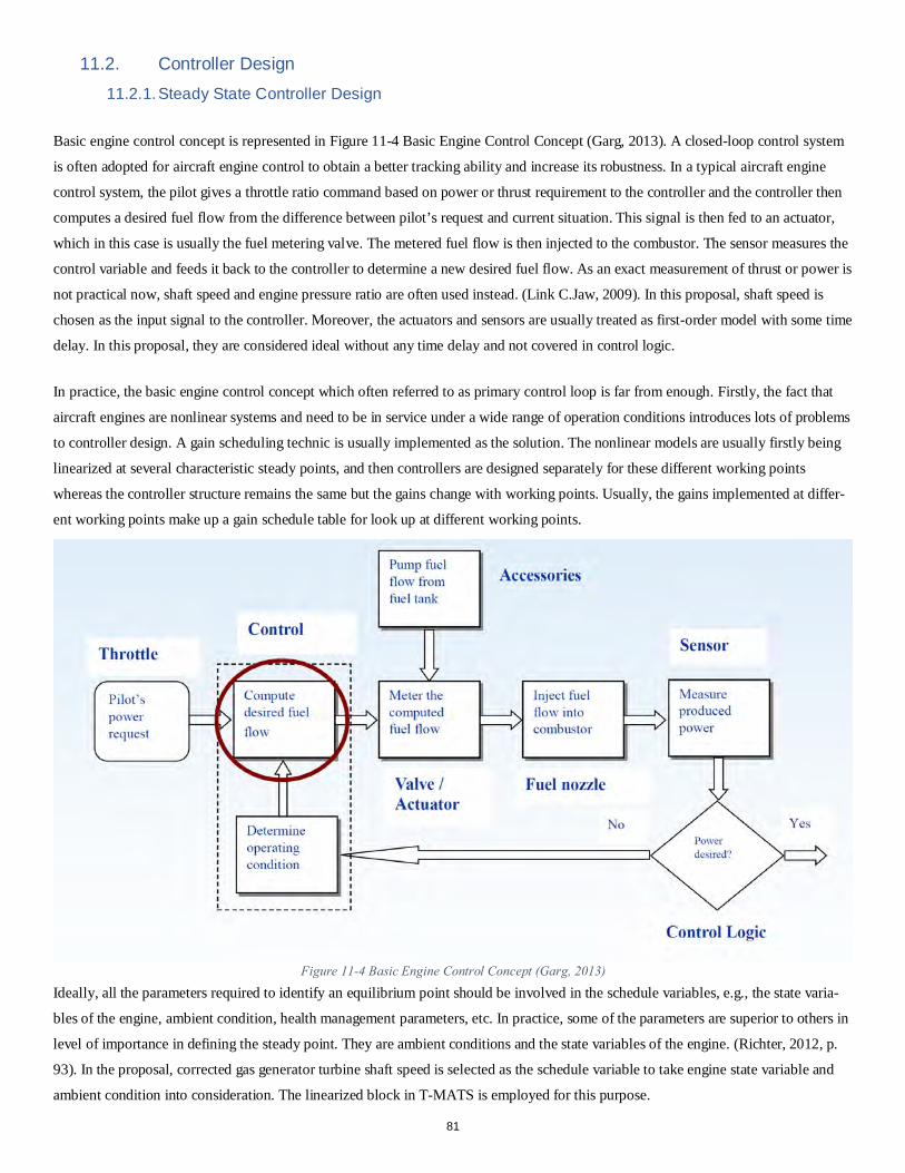
11.2. Controller Design 11.2.1. Steady State Controller Design
Basic engine control concept is represented in Figure 11-4 Basic Engine Control Concept (Garg, 2013). A closed-loop control system
is often adopted for aircraft engine control to obtain a better tracking ability and increase its robustness. In a typical aircraft engine
control system, the pilot gives a throttle ratio command based on power or thrust requirement to the controller and the controller then
computes a desired fuel flow from the difference between pilot’s request and current situation. This signal is then fed to an actuator,
which in this case is usually the fuel metering valve. The metered fuel flow is then injected to the combustor. The sensor measures the
control variable and feeds it back to the controller to determine a new desired fuel flow. As an exact measurement of thrust or power is
not practical now, shaft speed and engine pressure ratio are often used instead. (Link C.Jaw, 2009). In this proposal, shaft speed is
chosen as the input signal to the controller. Moreover, the actuators and sensors are usually treated as first-order model with some time
delay. In this proposal, they are considered ideal without any time delay and not covered in control logic.
In practice, the basic engine control concept which often referred to as primary control loop is far from enough. Firstly, the fact that
aircraft engines are nonlinear systems and need to be in service under a wide range of operation conditions introduces lots of problems
to controller design. A gain scheduling technic is usually implemented as the solution. The nonlinear models are usually firstly being
linearized at several characteristic steady points, and then controllers are designed separately for these different working points
whereas the controller structure remains the same but the gains change with working points. Usually, the gains implemented at differ-
ent working points make up a gain schedule table for look up at different working points.
Ideally, all the parameters required to identify an equilibrium point should be involved in the schedule variables, e.g., the state varia-
bles of the engine, ambient condition, health management parameters, etc. In practice, some of the parameters are superior to others in
level of importance in defining the steady point. They are ambient conditions and the state variables of the engine. (Richter, 2012, p.
93). In the proposal, corrected gas generator turbine shaft speed is selected as the schedule variable to take engine state variable and
ambient condition into consideration. The linearized block in T-MATS is employed for this purpose.
Figure 11-4 Basic Engine Control Concept (Garg, 2013)
81
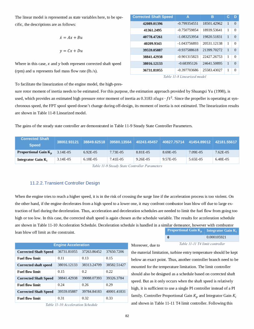
The linear model is represented as state variables here, to be spe-
cific, the descriptions are as follows:
�̇�𝑀 = 𝐴𝐴𝑀𝑀 +𝐵𝐵𝐵𝐵
𝑦𝑦 = 𝐶𝐶𝑀𝑀 + 𝐷𝐷𝐵𝐵
Where in this case, 𝑀𝑀 and 𝑦𝑦 both represent corrected shaft speed
(rpm) and 𝐵𝐵 represents fuel mass flow rate (lb./s).
To facilitate the linearization of the engine model, the high-pres-
sure rotor moment of inertia needs to be estimated. For this purpose, the estimation approach provided by Shuangxi Yu (1998), is
used, which provides an estimated high pressure rotor moment of inertia as 0.3183 𝑠𝑠𝑙𝑙𝐵𝐵𝑘𝑘𝑠𝑠 ∙ 𝑓𝑓𝑎𝑎2. Since the propeller is operating at syn-
chronous speed, the FPT spool speed doesn’t change during off-design, its moment of inertia is not estimated. The linearization results
are shown in Table 11-8 Linearized model.
The gains of the steady state controller are demonstrated in Table 11-9 Steady State Controller Parameters.
Corrected Shaft Speed
38002.93121 38849.62518 39580.13564 40243.45457 40827.75714 41454.89012 42181.55617
Proportional Gain 𝐊𝐊𝐩𝐩 3.14E-05 6.92E-05 7.73E-05 8.81E-05 8.69E-05 7.09E-05 7.62E-05
Integrator Gain 𝐊𝐊𝐢𝐢 3.14E-05 6.18E-05 7.41E-05 9.26E-05 9.57E-05 5.65E-05 6.48E-05
Table 11-9 Steady State Controller Parameters
11.2.2. Transient Controller Design
When the engine tries to reach a higher speed, it is in the risk of crossing the surge line if the acceleration process is too violent. On
the other hand, if the engine decelerates from a high speed to a lower one, it may confront combustor lean blow off due to large ex-
traction of fuel during the deceleration. Thus, acceleration and deceleration schedules are needed to limit the fuel flow from going too
high or too low. In this case, the corrected shaft speed is again chosen as the schedule variable. The results for acceleration schedule
are shown in Table 11-10 Acceleration Schedule. Deceleration schedule is handled in a similar demeanor, however with combustor
lean blow off limit as the constraint.
Moreover, due to
the material limitation, turbine entry temperature should be kept
below an exact point. Thus, another controller branch need to be
mounted for the temperature limitation. The limit controller
should also be designed as a schedule based on corrected shaft
speed. But as it only occurs when the shaft speed is relatively
high, it is sufficient to use a single PI controller instead of a PI
family. Controller Proportional Gain 𝐾𝐾𝑖𝑖 and Integrator Gain 𝐾𝐾𝐸𝐸
and shown in Table 11-11 T4 limit controller. Following this
Corrected Shaft Speed A B C D
42089.01396 -0.799354551 18501.42962 1 0
41361.2495 -0.750759854 18939.53641 1 0
40778.47261 -1.083253954 19820.51831 1 0
40209.9343 -1.043756893 20531.12138 1 0
39559.05887 -0.937588618 21399.70272 1 0
38841.42938 -0.901315823 22427.26753 1 0
38016.12133 -0.68395126 24641.50895 1 0
36731.81055 -0.397703686 25583.43027 1 0
Table 11-8 Linearized model
Engine Acceleration
Corrected Shaft Speed 36731.81055 37263.86452 37650.7206
Fuel flow limit 0.11 0.13 0.15
Corrected shaft speed 38016.12133 38313.24709 38582.51427
Fuel flow limit 0.15 0.2 0.22
Corrected Shaft Speed 38841.42938 39088.07393 39326.3784
Fuel flow limit 0.24 0.26 0.29
Corrected Shaft Speed 39559.05887 39784.84183 40001.41831
Fuel flow limit 0.31 0.32 0.33
Table 11-10 Acceleration Schedule
Proportional Gain 𝐊𝐊𝐩𝐩 Integrator Gain 𝐊𝐊𝐢𝐢
0 0.000105921
Table 11-11 T4 limit controller
82
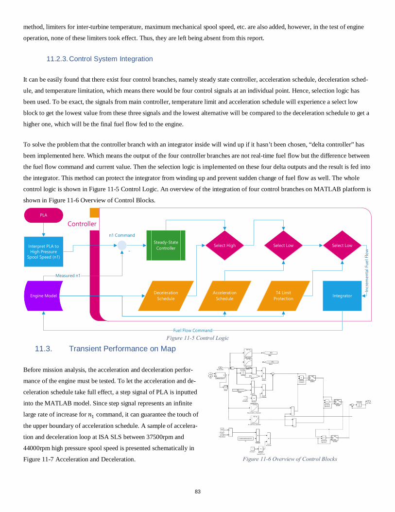
method, limiters for inter-turbine temperature, maximum mechanical spool speed, etc. are also added, however, in the test of engine
operation, none of these limiters took effect. Thus, they are left being absent from this report.
11.2.3. Control System Integration
It can be easily found that there exist four control branches, namely steady state controller, acceleration schedule, deceleration sched-
ule, and temperature limitation, which means there would be four control signals at an individual point. Hence, selection logic has
been used. To be exact, the signals from main controller, temperature limit and acceleration schedule will experience a select low
block to get the lowest value from these three signals and the lowest alternative will be compared to the deceleration schedule to get a
higher one, which will be the final fuel flow fed to the engine.
To solve the problem that the controller branch with an integrator inside will wind up if it hasn’t been chosen, “delta controller” has
been implemented here. Which means the output of the four controller branches are not real-time fuel flow but the difference between
the fuel flow command and current value. Then the selection logic is implemented on these four delta outputs and the result is fed into
the integrator. This method can protect the integrator from winding up and prevent sudden change of fuel flow as well. The whole
control logic is shown in Figure 11-5 Control Logic. An overview of the integration of four control branches on MATLAB platform is
shown in Figure 11-6 Overview of Control Blocks.
11.3. Transient Performance on Map
Before mission analysis, the acceleration and deceleration perfor-
mance of the engine must be tested. To let the acceleration and de-
celeration schedule take full effect, a step signal of PLA is inputted
into the MATLAB model. Since step signal represents an infinite
large rate of increase for 𝑠𝑠1 command, it can guarantee the touch of
the upper boundary of acceleration schedule. A sample of accelera-
tion and deceleration loop at ISA SLS between 37500rpm and
44000rpm high pressure spool speed is presented schematically in
Figure 11-7 Acceleration and Deceleration.
ControllerPLA
Interpret PLA to High Pressure
Spool Speed (n1)
n1 Command
-
Incr
emen
tal F
uel F
low
Engine Model
Fuel Flow Command
Measured n1
Steady-State Controller
Deceleration Schedule
Acceleration Schedule
T4 Limit Protection
Select High Select Low Select Low
Integrator
Figure 11-5 Control Logic
Figure 11-6 Overview of Control Blocks
83
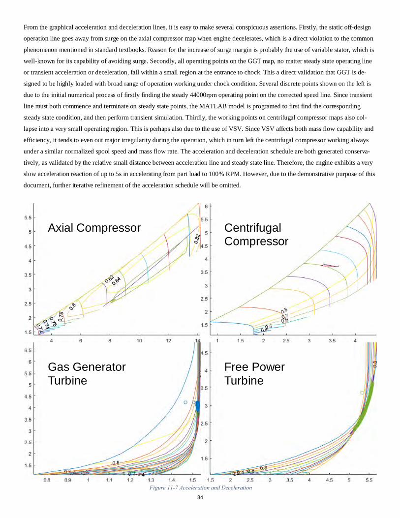
From the graphical acceleration and deceleration lines, it is easy to make several conspicuous assertions. Firstly, the static off-design
operation line goes away from surge on the axial compressor map when engine decelerates, which is a direct violation to the common
phenomenon mentioned in standard textbooks. Reason for the increase of surge margin is probably the use of variable stator, which is
well-known for its capability of avoiding surge. Secondly, all operating points on the GGT map, no matter steady state operating line
or transient acceleration or deceleration, fall within a small region at the entrance to chock. This a direct validation that GGT is de-
signed to be highly loaded with broad range of operation working under chock condition. Several discrete points shown on the left is
due to the initial numerical process of firstly finding the steady 44000rpm operating point on the corrected speed line. Since transient
line must both commence and terminate on steady state points, the MATLAB model is programed to first find the corresponding
steady state condition, and then perform transient simulation. Thirdly, the working points on centrifugal compressor maps also col-
lapse into a very small operating region. This is perhaps also due to the use of VSV. Since VSV affects both mass flow capability and
efficiency, it tends to even out major irregularity during the operation, which in turn left the centrifugal compressor working always
under a similar normalized spool speed and mass flow rate. The acceleration and deceleration schedule are both generated conserva-
tively, as validated by the relative small distance between acceleration line and steady state line. Therefore, the engine exhibits a very
slow acceleration reaction of up to 5s in accelerating from part load to 100% RPM. However, due to the demonstrative purpose of this
document, further iterative refinement of the acceleration schedule will be omitted.
Axial Compressor Centrifugal Compressor
Gas Generator Turbine
Free Power Turbine
Figure 11-7 Acceleration and Deceleration 84
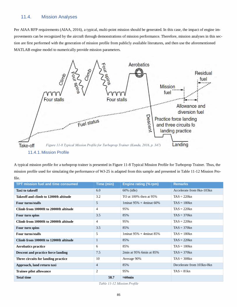
11.4. Mission Analyses
Per AIAA RFP requirements (AIAA, 2016), a typical, multi-point mission should be generated. In this case, the impact of engine im-
provements can be recognized by the aircraft through demonstrations of mission performance. Therefore, mission analyses in this sec-
tion are first performed with the generation of mission profile from publicly available literatures, and then use the aforementioned
MATLAB engine model to numerically provide mission parameters.
11.4.1. Mission Profile
A typical mission profile for a turboprop trainer is presented in Figure 11-8 Typical Mission Profile for Turboprop Trainer. Thus, the
mission profile used for simulating the performance of WJ-25 is adapted from this sample and presented in Table 11-12 Mission Pro-
file. TPT mission fuel and time consumed Time (min) Engine rating (% rpm) Remarks
Taxi to takeoff 6.0 60% (idle) Accelerate from 0kn-103kn
Takeoff and climb to 12000ft altitude 3.2 TO at 100% then at 95% TAS = 220kn
Four turns/stalls 5 1minat 95% + 4minat 60% TAS = 180kn
Climb from 10000ft to 20000ft altitude 4 95% TAS = 220kn
Four turn spins 3.5 85% TAS = 370kn
Climb from 10000ft to 20000ft altitude 4 95% TAS = 220kn
Four turn spins 3.5 85% TAS = 370kn
Four turns/stalls 5 1minat 95% + 4minat 85% TAS = 180kn
Climb from 10000ft to 12000ft altitude 1 85% TAS = 220kn
Aerobatics practice 6 85% TAS = 180kn
Descent and practice force landing 7.5 2min at 95% 6min at 85% TAS = 370kn
Three circuits for landing practice 10 Average 90% TAS = 308kn
Approach, land return taxi 4 85% Decelerate from 103kn-0kn
Trainee pilot allowance 2 95% TAS = 81kn
Total time 58.7 ≈60min
Table 11-12 Mission Profile
Figure 11-8 Typical Mission Profile for Turboprop Trainer (Kundu, 2016, p. 347)
85
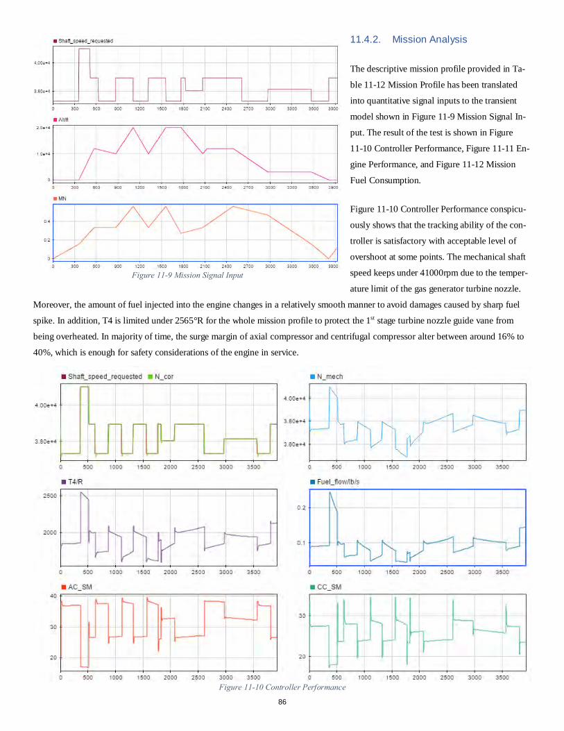
11.4.2. Mission Analysis
The descriptive mission profile provided in Ta-
ble 11-12 Mission Profile has been translated
into quantitative signal inputs to the transient
model shown in Figure 11-9 Mission Signal In-
put. The result of the test is shown in Figure
11-10 Controller Performance, Figure 11-11 En-
gine Performance, and Figure 11-12 Mission
Fuel Consumption.
Figure 11-10 Controller Performance conspicu-
ously shows that the tracking ability of the con-
troller is satisfactory with acceptable level of
overshoot at some points. The mechanical shaft
speed keeps under 41000rpm due to the temper-
ature limit of the gas generator turbine nozzle.
Moreover, the amount of fuel injected into the engine changes in a relatively smooth manner to avoid damages caused by sharp fuel
spike. In addition, T4 is limited under 2565°R for the whole mission profile to protect the 1st stage turbine nozzle guide vane from
being overheated. In majority of time, the surge margin of axial compressor and centrifugal compressor alter between around 16% to
40%, which is enough for safety considerations of the engine in service.
Figure 11-9 Mission Signal Input
Figure 11-10 Controller Performance
86
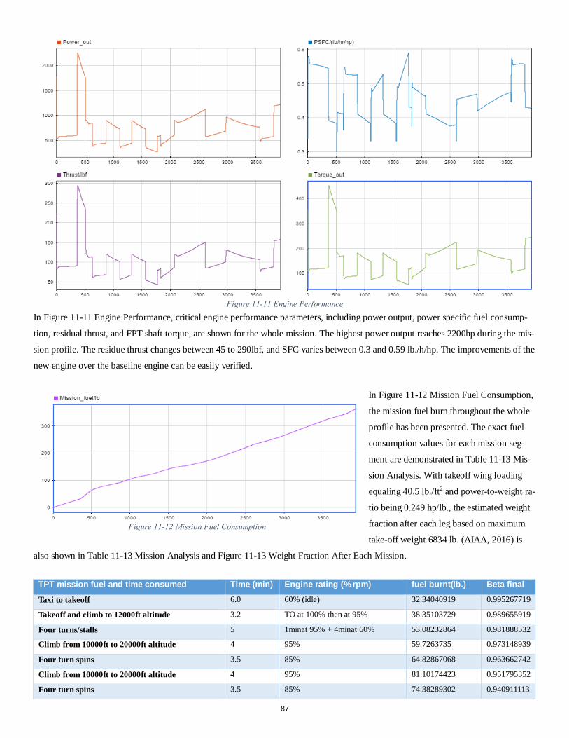
In Figure 11-11 Engine Performance, critical engine performance parameters, including power output, power specific fuel consump-
tion, residual thrust, and FPT shaft torque, are shown for the whole mission. The highest power output reaches 2200hp during the mis-
sion profile. The residue thrust changes between 45 to 290lbf, and SFC varies between 0.3 and 0.59 lb./h/hp. The improvements of the
new engine over the baseline engine can be easily verified.
In Figure 11-12 Mission Fuel Consumption,
the mission fuel burn throughout the whole
profile has been presented. The exact fuel
consumption values for each mission seg-
ment are demonstrated in Table 11-13 Mis-
sion Analysis. With takeoff wing loading
equaling 40.5 lb./ft2 and power-to-weight ra-
tio being 0.249 hp/lb., the estimated weight
fraction after each leg based on maximum
take-off weight 6834 lb. (AIAA, 2016) is
also shown in Table 11-13 Mission Analysis and Figure 11-13 Weight Fraction After Each Mission.
TPT mission fuel and time consumed Time (min) Engine rating (% rpm) fuel burnt(lb.) Beta final
Taxi to takeoff 6.0 60% (idle) 32.34040919 0.995267719
Takeoff and climb to 12000ft altitude 3.2 TO at 100% then at 95% 38.35103729 0.989655919
Four turns/stalls 5 1minat 95% + 4minat 60% 53.08232864 0.981888532
Climb from 10000ft to 20000ft altitude 4 95% 59.7263735 0.973148939
Four turn spins 3.5 85% 64.82867068 0.963662742
Climb from 10000ft to 20000ft altitude 4 95% 81.10174423 0.951795352
Four turn spins 3.5 85% 74.38289302 0.940911113
Figure 11-11 Engine Performance
Figure 11-12 Mission Fuel Consumption
87
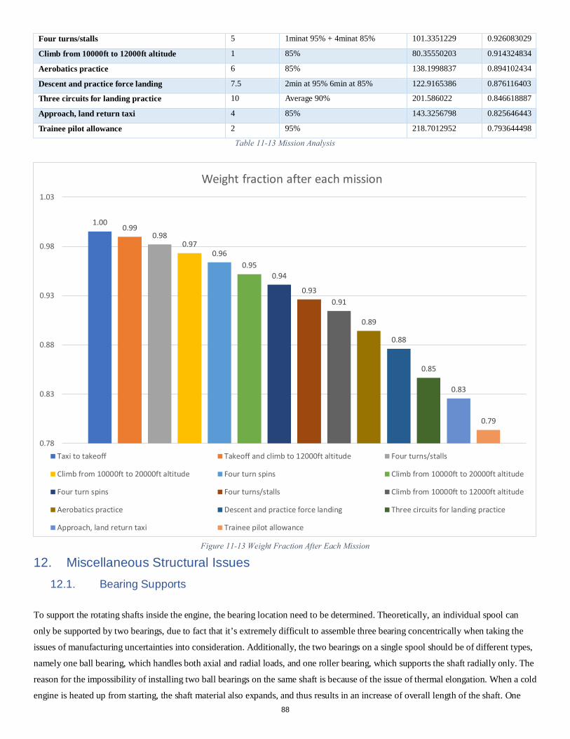
12. Miscellaneous Structural Issues12.1. Bearing Supports
To support the rotating shafts inside the engine, the bearing location need to be determined. Theoretically, an individual spool can
only be supported by two bearings, due to fact that it’s extremely difficult to assemble three bearing concentrically when taking the
issues of manufacturing uncertainties into consideration. Additionally, the two bearings on a single spool should be of different types,
namely one ball bearing, which handles both axial and radial loads, and one roller bearing, which supports the shaft radially only. The
reason for the impossibility of installing two ball bearings on the same shaft is because of the issue of thermal elongation. When a cold
engine is heated up from starting, the shaft material also expands, and thus results in an increase of overall length of the shaft. One
Four turns/stalls 5 1minat 95% + 4minat 85% 101.3351229 0.926083029
Climb from 10000ft to 12000ft altitude 1 85% 80.35550203 0.914324834
Aerobatics practice 6 85% 138.1998837 0.894102434
Descent and practice force landing 7.5 2min at 95% 6min at 85% 122.9165386 0.876116403
Three circuits for landing practice 10 Average 90% 201.586022 0.846618887
Approach, land return taxi 4 85% 143.3256798 0.825646443
Trainee pilot allowance 2 95% 218.7012952 0.793644498
Table 11-13 Mission Analysis
1.000.99
0.980.97
0.960.95
0.94
0.930.91
0.89
0.88
0.85
0.83
0.79
0.78
0.83
0.88
0.93
0.98
1.03
Weight fraction after each mission
Taxi to takeoff Takeoff and climb to 12000ft altitude Four turns/stalls
Climb from 10000ft to 20000ft altitude Four turn spins Climb from 10000ft to 20000ft altitude
Four turn spins Four turns/stalls Climb from 10000ft to 12000ft altitude
Aerobatics practice Descent and practice force landing Three circuits for landing practice
Approach, land return taxi Trainee pilot allowance
Figure 11-13 Weight Fraction After Each Mission
88
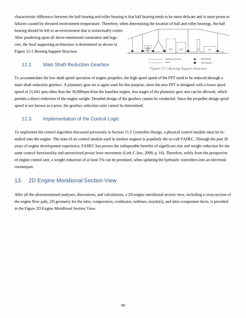
characteristic difference between the ball bearing and roller bearing is that ball bearing tends to be more delicate and is more prone to
failures caused by elevated environment temperature. Therefore, when determining the location of ball and roller bearings, the ball
bearing should be left in an environment that is instinctually cooler.
After pondering upon all above-mentioned constraints and lega-
cies, the final supporting architecture is determined as shown in
Figure 12-1 Bearing Support Structure.
12.2. Main Shaft Reduction Gearbox
To accommodate the low shaft speed operation of engine propeller, the high spool speed of the FPT need to be reduced through a
main shaft reduction gearbox. A planetary gear set is again used for this purpose, since the new FPT is designed with a lower spool
speed of 21,041 rpm other than the 30,000rpm from the baseline engine, less stages of the planetary gear sets can be allowed, which
permits a direct reduction of the engine weight. Detailed design of the gearbox cannot be conducted. Since the propeller design spool
speed is not known as a prior, the gearbox reduction ratio cannot be determined.
12.3. Implementation of the Control Logic
To implement the control algorithm discussed previously in Section 11.2 Controller Design, a physical control module must be in-
stalled onto the engine. The state of art control module used in modern engines is popularly the so-call FADEC. Through the past 30
years of engine development experience, FADEC has proven the indisputable benefits of significant size and weight reduction for the
same control functionality and unrestricted power lever movement (Link C.Jaw, 2009, p. 16). Therefore, solely from the perspective
of engine control unit, a weight reduction of at least 5% can be promised, when updating the hydraulic controllers into an electronic
counterpart.
13. 2D Engine Meridional Section View
After all the aforementioned analyses, discussions, and calculations, a 2D engine meridional section view, including a cross-section of
the engine flow path, 2D geometry for the inlet, compressors, combustor, turbines, nozzle(s), and inter-component ducts, is provided
in the Figure 2D Engine Meridional Section View.
ACCCGCTFPTGEARBOX
stationary structure
roters
ball bearing
roter bearing
Figure 12-1 Bearing Support Structure
89
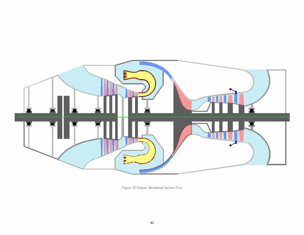
Figure 2D Engine Meridional Section View
90
14. References
AIAA. (2016). Candidate Engines for a Next Generation Single-Engine Turboprop Aircraft. AIAA Foundation Student Design
Competition 2016/17 Undergraduate Team – Engine.
Authur H. Lefebvre, D. R. (2010). Gas Tubine Combustion. Boca Raton: CRC Press.
Badger, M., Julien, A., LeBlanc, A., Moustapha, S., Prabhu, A., & Smailys, A. (1994). The PT6 Engine: 30 Years of Gas Turbine
Technology Evolution. ASME Journal of Engineering for Gas Turbine Engines and Power, 322-330.
Bansal, N. P. (2005). Handbook of Ceramic Composites. Boston: KLUWER ACADEMIC PUBLISHERS.
BASKHARONE, E. A. (2006). Principles of Turbomachinery in Air-Breathing Engines. Cambridge: Cambridge University Press.
Bullock, R. O., & Johnsen, I. A. (1965). AERODYNAMIC DESIGN OF AXIAL-FLOW COMPRESSORS NASA-SP-36. Cleveland:
Lewis Research Center.
Christopher O. Peterson, W. A. (2002). Performance of a Model Rich Burn-Quick Mix-Lean Burn Combustor at Elevated
Temperature and Pressure. NASA/CR--2002-211992.
Cumpsty, N. A. (2004). Compressor Aerodynamics. Malabar: Krieger Publishing Company.
EASA. (2016). TYPE-CERTIFICATE DATA SHEET No. EASA IM.E.038. Longueuil: European Aviation Safety Agency.
Europrop. (2017, 1 7). THE TP-400 D-6. Retrieved from Europrop International official website: http://www.europrop-int.com/the-tp-
400-d-6/
Gardiner, G. (2015, July 31). Aeroengine Composites, Part 1: The CMC invasion. Retrieved from Composites World:
http://www.compositesworld.com/articles/aeroengine-composites-part-1-the-cmc-invasion
Gardiner, G. (2015, August 31). Aeroengine Composites, Part 2: CFRPs expand. Retrieved from Composite World:
http://www.compositesworld.com/articles/aeroengine-composites-part-2-cfrps-expand
Garg, D. S. (2013). https://www.grc.nasa.gov/WWW/cdtb/aboutus/Fundamentals_of_Engine_Control.pdf. Retrieved from
https://www.grc.nasa.gov/.
GE Business & General Aviation. (2017). GE Advanced Turboprop. Retrieved from GE Aviation:
http://www.geaviation.com/bga/engines/advancedturboprop/
Glassman, J. (1972). Computer Program for Preliminary Design Analysis of Aixal-Flow Turbines. Cleveland: NASA Lewis Research
Center.
Glassman, J. (1992). Users Manual for Updated Computer Code for Axial-Flow Compressor Conceptual Design. Toledo: Lewis
Research Center.
91
Glassman, J. (1994). Turbine Design and Application NASA-SP-290. Washington, DC: Lewis Research Center.
H.G. Münzberg, J. K. (1977). Gasturbinen - Betriebsverhalten und Optimierung. New York: Springer-Verlag Berlin Heidelberg.
IPT. (2017, 1 9). MTR390-E. Retrieved from IPT official website:
http://www.itp.es/web/Sec_PL/wf_paginaPlana.aspx?IdMenu=361&Idioma=en-
GB&idReg=183&idSubmenu=452&idSubSubmenu=380&idP=20&idPS=1
ISO. (1975). Standard Atmosphere, ISO 2533. Geneva: International Organisation for Standardisation.
J. Seddon, E. G. (1999). Intake Aerodynamics. Victoria: Blackwell Science Ltd.
Kasper, J., & Balle, O. (2016, October 3). Pratt & Whitney Canada PT6A. Retrieved from FI-POWERWEB: http://www.fi-
powerweb.com/Engine/PW-CANADA-PT6A.html
Kundu, A. K. (2016). Theory and Practice of Aircraft Performance.
Kurtz, M. (1992). Ceramic Matrix Composites. Bericht der DKG.
Kurzke, J. (1992). Calculation of Installation Effects within Performance Computer Programs. In Steady and Transient Performance
Prediction of Gas Turbine Engines (pp. 127-145). Cambridge: Specialised Printing Services Limited.
Kurzke, J. (1995). Advanced User-friendly Gas Turbine Performance Calculations on A Personal Computer. ASME, 1-8.
Kurzke, J. (1996). How to Get Component Maps for Aircraft Gas Turbine Performance Calculations. ASME.
Kurzke, J. (2015). GasTurb 12: Design and Off-Design Performance of Gas Turbines. Aachen: GasTurb GmbH.
L. R. Reneau, J. P. (1967). Performance and Design of Straight, Two-Dimensional Diffusers. Journal of Basic Engineering, 141-150.
Link C.Jaw, J. D. (2009). Aircraft Engine Controls: Design, System Analysis and Health Monitoring. AIAA.
Loftin, J. (1980). Subsonic Aircraft: Evolution and the Matching of Size to Performance. NASA reference publication 1060.
Mattingly, J. D. (2002). Aircraft Engine Design. Reston: American Institute of Aeronautics and Astronautics.
Mellor, A. M. (1990). Design of Modern Turbine Combustors. San Diego: Academic Press Inc.
Michaux, A., Sauder, C., Camus, G., & Pailler, R. (2007). Young’s modulus, thermal expansion coefficient and fracture behavior of
selected Si–B–C based carbides in the 20–1200 ◦C temperature range as derived from the behavior of carbon fiber reinforced
microcomposites. Journal of the European Ceramic Society, 3551-3560.
MIL210. (1997). Climatic Information to Determine Design and Test Requirements for Military Equipment MIL210C, Rev C.
Massachusetts: US Department of Defense.
92
MIL-C-005011B. (1977). Military Specification, Chart Standard Aircraft Characteristics and Performance, Piloted Aircraft (Fixed
Wing). Wright-Patterson: USAF.
MIL-DTL-5624U. (1998). DETAIL SPECIFICATION TURBINE FUEL, AVIATION, GRADES JP-4 and JP-5. Patuxent River:
ASTM.
Muktinutalapati, N. R. (2016). Materials for Gas Turbines - An Overview. In E. Benini, Advances in Gas Turbine Technology (pp.
293-314). Rijeka: Intech.
NASA Glenn Research Center. (2014, 04 15). T-MATS: Toolbox for the Modeling and Analysis of Thermodynamic Systems. Retrieved
from Intelligent Control and Autonomy Branch: https://www.grc.nasa.gov/www/cdtb/software/t-mats.html
Norris, G. (2015, October 27). GE Unveils CMC Production Ramp-Up Plan. Retrieved from Aviation Week:
http://aviationweek.com/optimizing-engines-through-lifecycle/ge-unveils-cmc-production-ramp-plan
Philpot, M. G. (1992). Practical considerations in designing the engine cycle. AGARD Lecture Series 183 "Steady and Transient
Performance Prediction of Gas Turbine Engines", 26-49.
Pilatus. (2002). PC-21 Brochure. Stans: Pilatus Aircraft Ltd.
Rao, S. S. (2009). Random Search Methods. In S. S. Rao, Engineering Optimization: Theory and Practice (pp. 383-384). Hoboken:
John Wiley & Sons, Inc.
Richter, H. (2012). Advanced Control of Turbofan Engines. Springer.
Roskam, J. (1985). Airplane Design IV: Layout Design of Landing Gear and Systems. Ottawa: Roskam Aviation and Engineering
Corporation.
Roskam, J. (1985). Airplane Design Part I: Preliminary Sizing of Airplanes. Ottawa: Roskam Aviation and Engineering Corporation.
Roskam, J. (1985). Airplane Design Part VI: Preliminary Calculation of Aerodynamics, Thrust, and Power Characteristics. Ottawa:
Roskam Aviation and Engineering Corporation.
SAE. (1974). Gas Turbine Engine Performance Station Identification and Nomenclature. In Warrandale, Aerospace Recommended
Practice, ARP 755A. Pennsylvania: Society of Automotive Engineers.
SAE. (1974). Gas Turbine Engine Status Performance Presentation for Digital Computer Programs. In Warrandale, Aerospace
Recommended Practice, ARP 1211A. Pennsylvania: Society of Automotive Engineers.
SAE. (1989). Gas Turbine Engine Steady-State Performance Presentation for Digital Computer Programs. In Warrandale, Aerospace
Standard, AS681 Rev. E. Pennsylvania: Society of Automotive Engineers.
SAE. (1989). Gas Turbine Engine Transient Performance Presentation for Digital Computer Programs. In Warrandale, Aerospace
Recommended Practice, ARP 1257. Pennsylvania: Society of Automotive Engineers.
93
SAE. (1996). Gas Turbine Engine Interface Test Reduction Computer Programs. In Warrandale, Aerospace Recommended Practice,
ARP 1210A. Pennsylvania: Society of Automotive Engineers.
Saravanamuttoo, H., Rogers, G., Cohen, H., & Straznicky, P. (2009). Gas Turbine Theory. Harlow: Pearson Education Limited.
Schilke, P. (2004, August). Advanced Gas Turbine Materials and Coatings. Retrieved from GE Energy:
https://powergen.gepower.com/content/dam/gepower-pgdp/global/en_US/documents/technical/ger/ger-3569g-advanced-gas-
turbine-materials-coatings.pdf
Serovy, G. K. (1976). Compressor and Turbine Performance Prediction. In Modern Prediction Methods for Turbomachine
Performance (pp. 21-39). Technical Editing and Reproduction Ltd.: Munich.
Smith, S. (1965). A Simple Correlation of Turbine Efficiency. Journal of the Royal Aeronautical Society, 467–70.
SoftInWay. (n.d.). AxSTREAM® Tutorial. Burlington, MA, USA.
Stabe, R. G., Whitney, W. J., & Moffitt, T. P. (1984). Performance of a high-work low aspect ration turbine tested with a realistic
inlet radial temperature profile. Cleveland: NASA Lewis Research Center.
Stewart, W. L. (1962). A Study of Axial-Flow Turbine Efficiency Characteristics in Terms of Velocity Diagram Parameters. ASME.
Superalloy. (n.d.). Retrieved from Wikipedia: https://en.wikipedia.org/wiki/Superalloy
Tyner, T., & Sullivan, J. (1990). Design and Performance of a Small, High Speed Axial Compressor. AIAA paper, 90-1911.
Vinayak, P. (2000). Quasi-Static and Creep Behavior of Enhanced Sic/Sic Ceramic Matrix Composites. Master of Science in
Engineering Mechanics.
Viswanathan, R. (2003, July). Gas Turbine Blade Superalloy Material Property Handbook. Retrieved from EPRI:
http://www.epri.com/abstracts/Pages/ProductAbstract.aspx?ProductId=000000000001008477
Walsh, P. P., & Fletcher, P. (2004). Gas Turbine Performance. Oxford: Blackwell Science Ltd.
Wood, K. (2013, January 11). Ceramic-matrix composites heat up. Retrieved from Composite World:
http://www.compositesworld.com/articles/ceramic-matrix-composites-heat-up
Younghans, J. L., Johnson, J. E., & Csonka, S. J. (1994). A methodology to assess design uncertainty in selecting affordable gas
turbine technology. ASME Journal.
Авиабаза. (2017, 1 9). НК-62. Retrieved from Авиабаза: http://www.airbase.ru/alpha/rus/n/nk/62/
喻双喜. (1998). 航空发动机质量、质心及转动惯量的一种计算方法及应用. 中国航空学会重量工程专业学术会.
94