Embed Size (px)
Citation preview

Page 1 of 20 © Aquaveo 2012
WMS 9.1 Tutorial
Watershed Modeling – HEC-HMS Interface Learn how to setup a basic HEC-HMS model using WMS
Objectives Build a basic HEC-HMS model from scratch using a DEM, land use, and soil data. Compute the
geometric and hydrologic parameters required to run your HEC-HMS model. Divide your single
watershed into multiple sub-basins and define reach and reservoir routing between sub-basins.
Prerequisite Tutorials Watershed Modeling –
DEM Delineation
Required Components Data
Drainage
Map
Hydrology
Hydrologic Models
Time 30-60 minutes
v. 9.1
Page 2 of 20 © Aquaveo 2012
1 Contents
1 Contents ............................................................................................................................... 2 2 Introduction ......................................................................................................................... 2 3 Objectives ............................................................................................................................. 3 4 Delineating the Watershed ................................................................................................. 3
4.1 Create Land Use and Soil Coverages ........................................................................... 3 4.2 Open the Soils Data ...................................................................................................... 3 4.3 Join Soils Database File Table to Shapefile Table ....................................................... 4 4.4 Convert Soil Shapefile Data to Feature Objects ........................................................... 4 4.5 Open the Land Use Data .............................................................................................. 5 4.6 Convert/Set the Projection System of the Data ............................................................ 5 4.7 Delineate the Watershed ............................................................................................... 6
5 Single Basin Analysis .......................................................................................................... 8 5.1 Setting up the Job Control ............................................................................................ 8 5.2 Setting up the Meteorological Data .............................................................................. 8 5.3 Setting up the Basin Data Parameters .......................................................................... 9 5.4 Running HEC-HMS ................................................................................................... 10
6 Computing the CN Using Land Use and Soils Data ....................................................... 12 6.1 Computing a Composite CN ...................................................................................... 12 6.2 Running HEC-HMS ................................................................................................... 12
7 Adding Sub-basins and Routing ...................................................................................... 13 7.1 Delineating the Sub-basin .......................................................................................... 13 7.2 Updating the Basin Parameters .................................................................................. 15 7.3 Setting up the Routing Parameters ............................................................................. 16 7.4 Running HEC-HMS ................................................................................................... 17
8 Modeling a Reservoir in HEC-HMS ................................................................................ 18 8.1 Defining a Reservoir in Combination with Routing ................................................... 18 8.2 Setting up the Reservoir Routing Parameters ............................................................. 18 8.3 Running HEC-HMS ................................................................................................... 19
9 Conclusion.......................................................................................................................... 20
2 Introduction
WMS includes a graphical interface to HEC-HMS. This tutorial is similar to the HEC-1
tutorial. Geometric attributes such as areas, lengths, and slopes are computed
automatically from the digital watershed. Parameters such as loss rates, base flow, unit
hydrograph method, and routing data are entered through a series of interactive dialog
boxes. Once the parameters needed to define an HMS model have been entered, an input
file with the proper format for HMS can be written automatically.
Since only parts of the HMS input file are defined in this chapter, you are encouraged to
explore the different available options of each dialog, being sure to select the given
method and values before exiting the dialog. Unlike HEC-1, you will need to export the
HMS files from WMS and then run the HMS graphical user interface to view the results.
In order to do this you should have the most recent version of HMS installed.

WMS Tutorials Watershed Modeling – HEC-HMS Interface
Page 3 of 20 © Aquaveo 2012
3 Objectives
As a review, you will delineate a watershed from a DEM. You will then develop a
simple, single basin model using the delineated watershed to derive many of the
parameters. Land use and soil shapefiles (downloaded from the Internet) will be used to
develop a SCS curve number (CN) value. After establishing the initial HMS model, other
variations will be developed, including defining multiple basins with reach routing and
including a reservoir with storage routing.
4 Delineating the Watershed
Since the land use, soil type, and DEM data for our watershed all originate in the
Geographic coordinate system, we will begin by opening them together and converting
them to UTM coordinates. The land use and soil type data were downloaded from the
Environmental Protection Agency (EPA) website. The DEM data used for this watershed
were previously downloaded from the National Elevation Dataset website as was
demonstrated in the DEM Basics exercise (Volume 1, chapter 4).
1. Close all instances of WMS
2. Open WMS
3. Select File | Open
4. Locate the hec-1 folder in your tutorial files. If you have used default
installation settings in WMS, the tutorial files will be located in \My
documents\WMS 9.1\Tutorials\.
5. Select NED GRIDFLOAT Header (*.hdr) from the Files of type list of file
filters
6. Open “67845267.hdr”
7. Select OK
8. When prompted if you want to change projection of the data, select No
4.1 Create Land Use and Soil Coverages
1. Right-click on the Coverages folder in the Project Explorer
2. Select New Coverage
3. Change the coverage type to Land Use
4. Select OK
5. Create a new coverage once again and set its coverage type to Soil Type
4.2 Open the Soils Data
1. Make sure the Soil Type coverage is active in the Project Explorer
2. Right-click on GIS Layers in the Project Explorer and select Add Shapefile
Data
3. Open “statsgo.shp”

WMS Tutorials Watershed Modeling – HEC-HMS Interface
Page 4 of 20 © Aquaveo 2012
4. If a dialog appears regarding changing projection, select No
5. Right-click on statsgo.shp layer in the Project Explorer
6. Select Open Attribute Table
Notice that the table has three fields named AREA, PERIMETER, and MUID
7. Select OK
4.3 Join Soils Database File Table to Shapefile Table
1. Right-click on statsgo.shp in the Project Explorer
2. Select Join Table to Layer
3. Open “statsgoc.dbf”
4. Ensure that Shapefile Join Field and Table Join Field are both set to MUID
5. Change the Table Data Field to HYDGRP
6. Select OK
7. Right-click on statsgo.shp in the Project Explorer
8. Select Open Attribute Table
Notice that the HYDGRP field is now a part of the shapefile.
9. Select OK
4.4 Convert Soil Shapefile Data to Feature Objects
1. Choose the Select Shapes tool
2. Draw a selection box around the DEM extents
3. Select Mapping | Shapes -> Feature Objects
4. Select Next
This window shows all of the attribute fields in the soils shape file. Because this file was
derived from a standard NRCS statsgo file you will notice that the hydrologic soil groups
field is named HYDGRP and so WMS will automatically map this to be the soil type. If
the attribute field were named anything other than HYDGRP then you would have to
manually map it using the drop down list in the spreadsheet.
5. Make sure the HYDGRP field is mapped to the SCS soil type attribute
6. Select Next
7. Select Finish
8. Clear the selected polygons by single-clicking somewhere beyond the
extents of the shapefile polygons
9. Hide the statsgo.shp file by toggling off its check box in the Project
Explorer

WMS Tutorials Watershed Modeling – HEC-HMS Interface
Page 5 of 20 © Aquaveo 2012
4.5 Open the Land Use Data
1. Select the Land Use coverage in the Project Explorer to designate it as the
active coverage
2. Right-click on GIS Layers in the Project Explorer and select Add Shapefile
Data
3. Open “l_richut.shp”
4. Choose the Select Shapes tool
5. Draw a selection box around the DEM extents
6. Select Mapping | Shapes -> Feature Objects
7. Select Next
8. Make sure the LUCODE field is mapped to the Land use attribute
9. Select Next
10. Select Finish
11. Hide the l_richut.shp file by toggling off its check box in the Project
Explorer
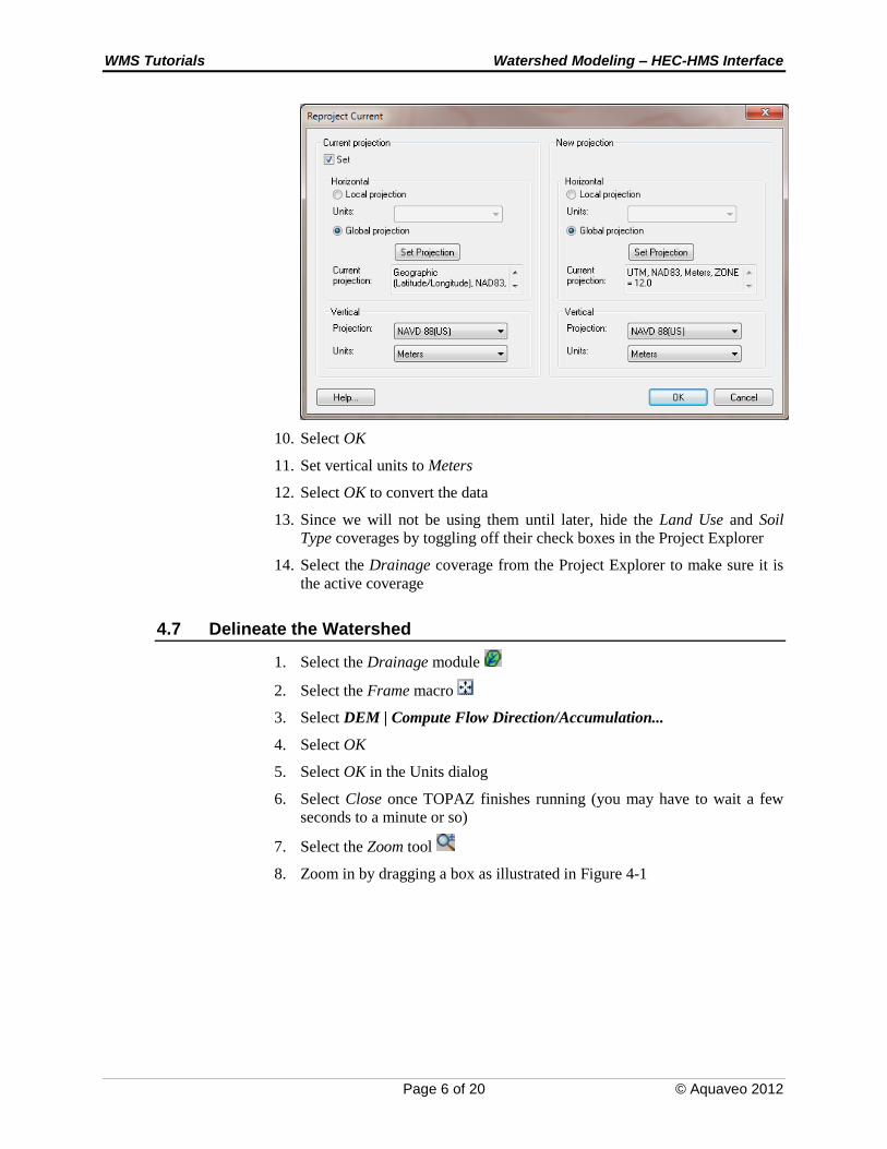
4.6 Convert/Set the Projection System of the Data
1. Select Edit | Reproject.
2. Select the Set option in the Current Projection section of the Reproject
Current dialog
3. Select Set Projection
4. Set Projection to Geographic, and Datum to NAD 83
5. Select OK
6. Set Vertical Units to Meters
7. In the New Projection section select Global Projection
8. Select Set Projection
9. Set Projection to UTM, Datum to NAD 83, Planar Units to METERS, and
Zone to 12 (114°W - 108°W – Northern Hemisphere)
WMS Tutorials Watershed Modeling – HEC-HMS Interface
Page 6 of 20 © Aquaveo 2012
10. Select OK
11. Set vertical units to Meters
12. Select OK to convert the data
13. Since we will not be using them until later, hide the Land Use and Soil
Type coverages by toggling off their check boxes in the Project Explorer
14. Select the Drainage coverage from the Project Explorer to make sure it is
the active coverage
4.7 Delineate the Watershed
1. Select the Drainage module
2. Select the Frame macro
3. Select DEM | Compute Flow Direction/Accumulation...
4. Select OK
5. Select OK in the Units dialog
6. Select Close once TOPAZ finishes running (you may have to wait a few
seconds to a minute or so)
7. Select the Zoom tool
8. Zoom in by dragging a box as illustrated in Figure 4-1

WMS Tutorials Watershed Modeling – HEC-HMS Interface
Page 7 of 20 © Aquaveo 2012
Figure 4-1: Zoom in on the area bounded by the rectangle above
9. Select the Create Outlet Point tool
10. Create a new outlet point where the tributary you just zoomed in on
separates from the main stream as illustrated by the arrow in Figure 4-1.
Make certain that the outlet point is on the tributary and not part of the
main stream. Also, the outlet needs to be inside one of the flow
accumulation (blue) cells. WMS will move the outlet to the nearest flow
accumulation cell if you do not click right in one of the flow accumulations
cells.
11. Select the Frame macro
12. Select DEM | Delineate Basins Wizard
13. Select Delineate Watershed
14. Select Close
You have now completed the delineation of a single watershed. In order to make the view
clearer for defining the hydrologic model you can turn off many of the DEM and other
display options.
15. Right-click on DEM in the Project Explorer and select Display Options
16. In the DEM Data options, toggle off the display for Watershed, Stream,
Flow Accumulation, and DEM Contours
17. In the Map Data options, toggle Vertices off
18. Select OK

WMS Tutorials Watershed Modeling – HEC-HMS Interface
Page 8 of 20 © Aquaveo 2012
5 Single Basin Analysis
The first simulation will be defined for a single basin. You will need to enter the global,
or Job Control parameters as well as basin and meteorological data.
5.1 Setting up the Job Control
Most of the parameters required for a HEC-HMS model are defined for basins, outlets,
and reaches. However, there are some “global” parameters that control the overall
simulation and are not specific to any basin or reach in the model. These parameters are
defined in the WMS interface using the Job Control dialog.
1. Switch to the Hydrologic Modeling module
2. HEC-1 should be the default model, so change the default model to HEC-
HMS by selecting it from the drop down list of models found in the Edit
Window
3. Select HEC-HMS | Job Control
4. Enter “Clear Creek Tributary” in the Name: field
5. In the Description: field you can enter Your name
By default the simulation is set to run for 24 hours starting from today’s date at 15 minute
intervals. We want to run this simulation for 25 hours at five minute intervals.
6. Add one hour to the Ending time
7. Change the Time interval to 5 Minutes
8. Select the Basin Options tab
9. Enter “Clear Creek Tributary” in the Name: field
10. Set the Basin Model Units to US customary (English), which should
already be the default
Setting the computation units DOES NOT cause any units conversion to take place. You
are simply telling HEC-1 that you will provide input units in English units (sq. miles for
area, inches for rain, feet/miles for length) and expect results of computation to be in
English units (cfs). If you specify Metric then you must ensure that input units are metric
(sq. kilometers, mm for rain, meters/kilometers for length) and results will be in metric
(cms).
11. Select the Meteorological Options tab
12. Enter “Clear Creek Tributary” in the Name: field
You will note that HEC-HMS includes advanced options for long term simulation and
local inflows at junctions, but we will not explore these options in this model.
13. Select OK
5.2 Setting up the Meteorological Data
In HEC-1 precipitation is handled as a Basin Data attribute, however for HEC-HMS
precipitation is defined separately in the Meteorological Data. This is because of the

WMS Tutorials Watershed Modeling – HEC-HMS Interface
Page 9 of 20 © Aquaveo 2012
ability of HEC-HMS to model long term simulations that require additional information
and often a lot more input.
1. Select HEC-HMS | Meteorological Parameters
2. Set the Precipitation Method to SCS Hypothetical Storm
3. Set the Storm Selection to Type II
4. Set the Storm Depth to 1.8 (inches)
5. Select OK
5.3 Setting up the Basin Data Parameters
In the first simulation you will treat the entire watershed as a single basin.
1. Select the Select Basin tool
2. Double-click on the brown basin icon labeled 1B. Double-clicking on a
basin or outlet icon always brings up the parameter editor dialog for the
current model (in this case HEC-HMS)
3. Notice that the area has been calculated (in this case in sq. miles because
we are performing calculations in English units).
4. Change the name to CCTrib
5. Enter “Main Branch” in the description.
Displaying and Showing options allows you to see only those variables for which you
wish to enter data. For example in this case toggling on the Loss Rate Method allows
you to pick which method you want to use (in this case the method we want is the
default). You then toggle the display for the different parameters associated with a given
methodology from the show column. In our case we can now see in the Properties
window the Loss Rate Method and the parameters for the SCS Curve Number method.
The HMS-Properties window is versatile in that it allows you to see properties for all or
selected basins, junctions, reaches, reservoirs, etc.
6. Toggle on the Display of the Loss Rate Method option
7. Toggle the SCS Curve Number from the Show column in the Display
options window
8. Enter an SCS Curve Number of 70. We will compute a CN value from
actual land use and soil files later.
For the SCS CN method initial losses are estimated as 20% of the maximum storage
value computed from the CN when the initial loss is zero. If you wish to override this
computation then you would enter a value other than zero. For now we will assume there
is no impervious area.
9. Toggle on the Display of the Transform option (you may have to scroll
vertically in the Display options window)
10. Show the SCS parameters by toggling this option on in the Display options
window)
WMS Tutorials Watershed Modeling – HEC-HMS Interface
Page 10 of 20 © Aquaveo 2012
11. Scroll horizontally in the Properties window and choose the Compute
button under Basin Data (the SCS transform method is the default)
12. Set the Computation Type to Compute Lag Time (the default)
13. Set the Method drop down list to SCS Method (near the bottom of the list)
14. Select OK to update the computed lag time for the SCS dimensionless
method (scroll horizontally to view if you would like)
15. Select OK
You now have all of the parameters set to run a single basin analysis.
5.4 Running HEC-HMS
Whenever you run an HEC-HMS simulation, you must save the information created in
WMS to HEC-HMS files and then load it as a project in HEC-HMS. This tutorial is not a
comprehensive review of HEC-HMS but should give you an idea of how to open a
project created by WMS, run an analysis and view some basic results.
1. Right click on Drainage Coverage Tree in the Project Explorer and select
Save HMS File or Select HEC-HMS |Save HMS File
2. Change the HMS project file to CCTrib
3. Start HEC-HMS on your computer
4. Select File |Open
5. Select the Browse button and browse to the location where you just saved
your HMS Project from WMS (by default this will be in the hec-1
directory of your tutorial files)
6. Select the CCTrib.hms project file
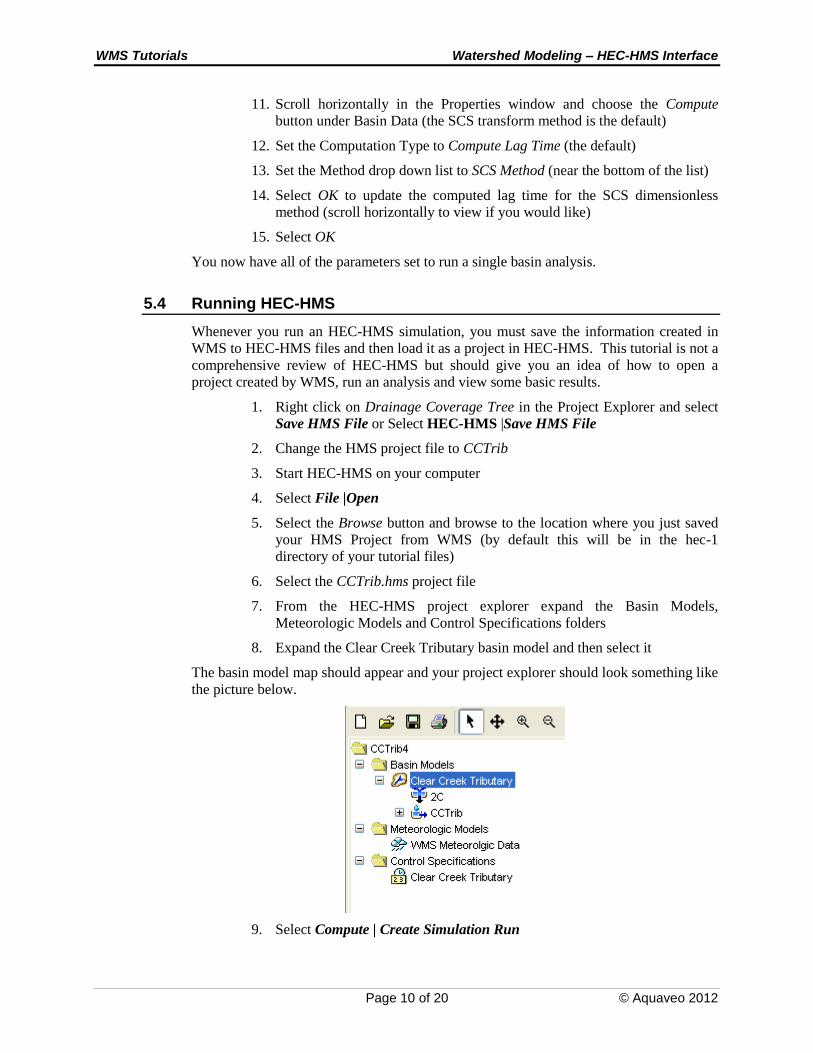
7. From the HEC-HMS project explorer expand the Basin Models,
Meteorologic Models and Control Specifications folders
8. Expand the Clear Creek Tributary basin model and then select it
The basin model map should appear and your project explorer should look something like
the picture below.
9. Select Compute | Create Simulation Run
WMS Tutorials Watershed Modeling – HEC-HMS Interface
Page 11 of 20 © Aquaveo 2012
10. Change the Run Name to CCTrib 1
11. Click Next, Next, Next and Finish to set up the simulation run
12. Select Compute | Select Run | Select Run -> CCTrib 1
13. Select Compute | Compute Run [CCTrib 1] or the Compute Current Run
macro
14. When finished computing select Close
15. Select the CCTrib basin under the Clear Creek Tributary basin model from
the HEC-HMS project explorer
16. Select Results | Global Summary Table and explore
17. Select Results | Element Graph and explore
18. Select Results | Element Summary Table and explore
19. Select Results | Element Time-Series Table and explore
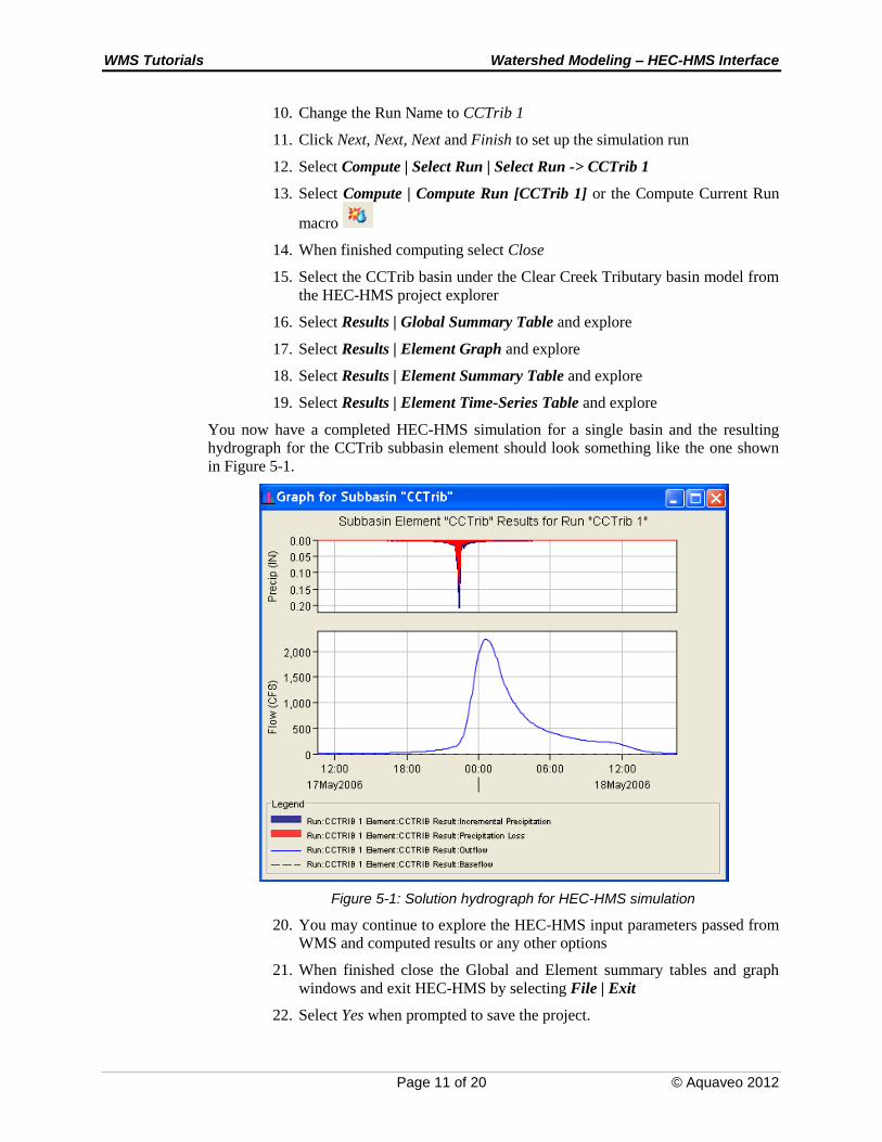
You now have a completed HEC-HMS simulation for a single basin and the resulting
hydrograph for the CCTrib subbasin element should look something like the one shown
in Figure 5-1.
Figure 5-1: Solution hydrograph for HEC-HMS simulation
20. You may continue to explore the HEC-HMS input parameters passed from
WMS and computed results or any other options
21. When finished close the Global and Element summary tables and graph
windows and exit HEC-HMS by selecting File | Exit
22. Select Yes when prompted to save the project.

WMS Tutorials Watershed Modeling – HEC-HMS Interface
Page 12 of 20 © Aquaveo 2012
6 Computing the CN Using Land Use and Soils Data
In the initial simulation you estimated a CN, but with access to the Internet it is simple to
compute a composite CN based on digital land use and soils files. This was demonstrated
in more detail in the Advanced Feature Objects exercise (Volume 1, chapter 6), but you
will go through the steps here as a review.
6.1 Computing a Composite CN
At the beginning of this tutorial you loaded digital land use and soils files for the purpose
of calculating a CN. In addition to this data, you must have a table defined that relates
CN values for each of the four different hydrologic soil groups (A, B, C, D) for each land
use. This is described in detail at the gsda website
(http://www.xmswiki.com/wiki/GSDA:GSDA), and in the Advanced Feature Objects
exercise (Volume 1, chapter 6). For this exercise you will read in an existing file (you can
examine it in a text editor if you wish) and compute the CN numbers.
1. While it is not necessary to have the Land Use and Soil Type coverages
displayed for the computations to work you may wish to make them visible
again by toggling on their check boxes in the Project Explorer
2. Select the Drainage coverage to make sure it is the active coverage
3. Select the Hydrologic Modeling module
4. Select Calculators | Compute GIS Attributes
5. Select the Import button to load the mapping table
6. Select OK to overwrite the current definition
7. Find and open the file named “scsland.tbl”
8. Select OK to compute the CN from the land use and soils layers
You should see the computed CN displayed in the Runoff Curve Number Report and
above the area label in the WMS graphics window.
9. Close the Runoff Curve Number Report
6.2 Running HEC-HMS
You can now run another simulation to compare the results with the modified CN value.
1. Right click on Drainage Coverage Tree in the Project Explorer and select
Save HMS File or Select HEC-HMS |Save HMS File
2. Name the HMS project file CCTribCN and Save
3. Start HEC-HMS on your computer
4. Select File |Open
5. Select the Browse button and browse to the location where you just saved
your HMS Project from WMS (by default this will be in the hec-1
directory of your tutorial files)
6. Select the CCTribCN.hms project file

WMS Tutorials Watershed Modeling – HEC-HMS Interface
Page 13 of 20 © Aquaveo 2012
7. From the HEC-HMS project explorer expand the Basin Models,
Meteorologic Models and Control Specifications folders
8. Expand the Clear Creek Tributary basin model and then select it
9. Select Compute | Create Simulation Run
10. Change the Run Name to CCTribCN 1
11. Click Next, Next, Next, and Finish to set up the Run
12. Select Compute | Select Run | CCTribCN 1
13. Select Compute | Compute Run [CCTribCN 1] or the Compute Current
Run macro
14. When finished computing select Close
15. Select the CCTrib basin under the Clear Creek Tributary basin model from
the HEC-HMS project explorer
16. Select Results | Global Summary Table and explore
17. Select Results | Element Graph and explore
18. Select Results | Element Summary Table and explore
19. Select Results | Element Time-Series Table and explore
You may continue to explore the HEC-HMS input parameters passed from WMS and
computed results or any other options
20. When finished close the Global and Element summary tables and graph
windows and exit HEC-HMS by selecting File | Exit
21. Select Yes when prompted to save the project.
7 Adding Sub-basins and Routing
You will now subdivide the watershed into two upper basins and one lower basin and
define routing for the reaches that connect the upper basins to the watershed outlet.
7.1 Delineating the Sub-basin
1. Select the Zoom tool
2. Create a zoom box around the region identified by a box in Figure 7-1
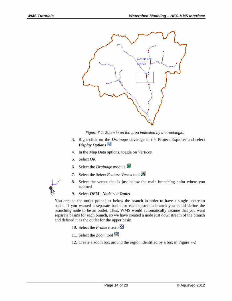
WMS Tutorials Watershed Modeling – HEC-HMS Interface
Page 14 of 20 © Aquaveo 2012
Figure 7-1: Zoom in on the area indicated by the rectangle.
3. Right-click on the Drainage coverage in the Project Explorer and select
Display Options
4. In the Map Data options, toggle on Vertices
5. Select OK
6. Select the Drainage module
7. Select the Select Feature Vertex tool
8. Select the vertex that is just below the main branching point where you
zoomed
9. Select DEM | Node <-> Outlet
You created the outlet point just below the branch in order to have a single upstream
basin. If you wanted a separate basin for each upstream branch you could define the
branching node to be an outlet. Thus, WMS would automatically assume that you want
separate basins for each branch, so we have created a node just downstream of the branch
and defined it as the outlet for the upper basin.
10. Select the Frame macro
11. Select the Zoom tool
12. Create a zoom box around the region identified by a box in Figure 7-2
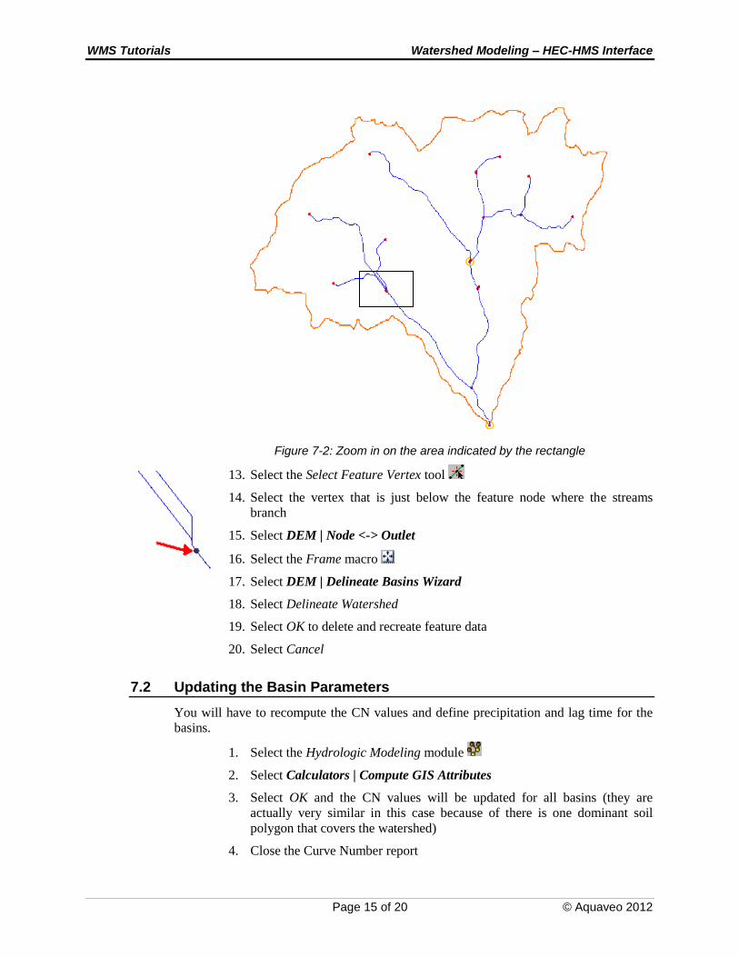
WMS Tutorials Watershed Modeling – HEC-HMS Interface
Page 15 of 20 © Aquaveo 2012
Figure 7-2: Zoom in on the area indicated by the rectangle
13. Select the Select Feature Vertex tool
14. Select the vertex that is just below the feature node where the streams
branch
15. Select DEM | Node <-> Outlet
16. Select the Frame macro
17. Select DEM | Delineate Basins Wizard
18. Select Delineate Watershed
19. Select OK to delete and recreate feature data
20. Select Cancel
7.2 Updating the Basin Parameters
You will have to recompute the CN values and define precipitation and lag time for the
basins.
1. Select the Hydrologic Modeling module
2. Select Calculators | Compute GIS Attributes
3. Select OK and the CN values will be updated for all basins (they are
actually very similar in this case because of there is one dominant soil
polygon that covers the watershed)
4. Close the Curve Number report
WMS Tutorials Watershed Modeling – HEC-HMS Interface
Page 16 of 20 © Aquaveo 2012
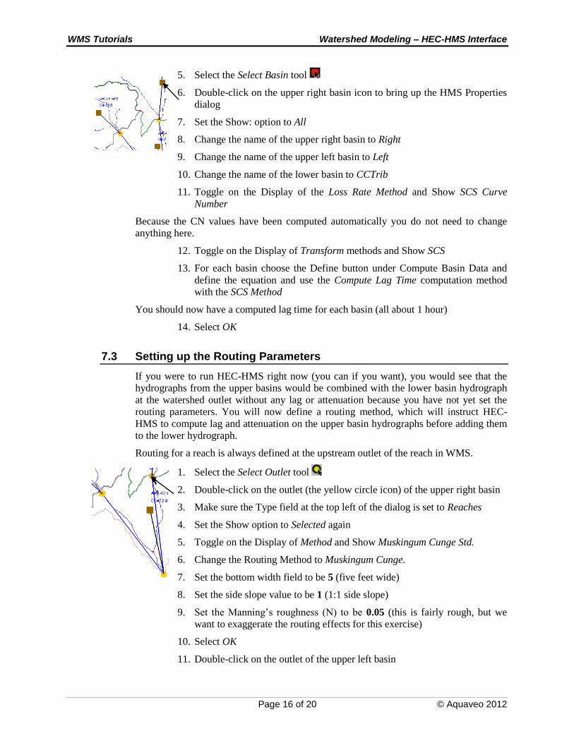
5. Select the Select Basin tool
6. Double-click on the upper right basin icon to bring up the HMS Properties
dialog
7. Set the Show: option to All
8. Change the name of the upper right basin to Right
9. Change the name of the upper left basin to Left
10. Change the name of the lower basin to CCTrib
11. Toggle on the Display of the Loss Rate Method and Show SCS Curve
Number
Because the CN values have been computed automatically you do not need to change
anything here.
12. Toggle on the Display of Transform methods and Show SCS
13. For each basin choose the Define button under Compute Basin Data and
define the equation and use the Compute Lag Time computation method
with the SCS Method
You should now have a computed lag time for each basin (all about 1 hour)
14. Select OK
7.3 Setting up the Routing Parameters
If you were to run HEC-HMS right now (you can if you want), you would see that the
hydrographs from the upper basins would be combined with the lower basin hydrograph
at the watershed outlet without any lag or attenuation because you have not yet set the
routing parameters. You will now define a routing method, which will instruct HEC-
HMS to compute lag and attenuation on the upper basin hydrographs before adding them
to the lower hydrograph.
Routing for a reach is always defined at the upstream outlet of the reach in WMS.
1. Select the Select Outlet tool
2. Double-click on the outlet (the yellow circle icon) of the upper right basin
3. Make sure the Type field at the top left of the dialog is set to Reaches
4. Set the Show option to Selected again
5. Toggle on the Display of Method and Show Muskingum Cunge Std.
6. Change the Routing Method to Muskingum Cunge.
7. Set the bottom width field to be 5 (five feet wide)
8. Set the side slope value to be 1 (1:1 side slope)
9. Set the Manning’s roughness (N) to be 0.05 (this is fairly rough, but we
want to exaggerate the routing effects for this exercise)
10. Select OK
11. Double-click on the outlet of the upper left basin

WMS Tutorials Watershed Modeling – HEC-HMS Interface
Page 17 of 20 © Aquaveo 2012
12. Make sure the Type field at the top left of the dialog is set to Reaches
13. Change the Routing Method to Muskingum Cunge.
14. Set the bottom width field to be 5 (five feet wide)
15. Set the side slope value to be 1 (1:1 side slope)
16. Set the Manning’s roughness (N) to be 0.05 (this is fairly rough, but we
want to exaggerate the routing effects for this exercise)
17. Select OK
7.4 Running HEC-HMS
You now have everything defined to run a three basin HEC-HMS analysis that includes
routing the upper basins through the reaches connecting them to the watershed outlet.
1. Right click on Drainage Coverage Tree in the Project Explorer and select
Save HMS File or Select HEC-HMS |Save HMS File
2. Name the HMS project file CCTribRoute and Save
3. Start HEC-HMS on your computer
4. Select File |Open
5. Select the Browse button and browse to the location where you just saved
your HMS Project from WMS (by default this will be in the hec-1
directory of your tutorial files)
6. Select the CCTribRoute.hms project file
7. From the HEC-HMS project explorer expand the Basin Models,
Meteorologic Models and Control Specifications folders
8. Expand the Clear Creek Tributary basin model and then select it
9. Select Compute | Create Simulation Run
10. Change the Run Name to CCTribRoute 1
11. Click Next, Next, Next, and Finish to set up the simulation run
12. Select Compute | Select Run | Select Run CCTribRoute 1
13. Select Compute | Compute Run [CCTribRoute 1] or the Compute Current
Run macro
14. When finished computing select Close
15. Select different elements (basins, junctions, reaches) and view results
16. Select Results | Global Summary Table and explore
17. Select Results | Element Graph and explore
18. Select Results | Element Summary Table and explore
19. Select Results | Element Time-Series Table and explore
You may continue to explore the HEC-HMS input parameters passed from WMS and
computed results or any other options

WMS Tutorials Watershed Modeling – HEC-HMS Interface
Page 18 of 20 © Aquaveo 2012
20. When finished close the Global and Element summary tables and graph
windows and exit HEC-HMS by selecting File | Exit
21. Select Yes when prompted to save the project.
8 Modeling a Reservoir in HEC-HMS
There is an existing small reservoir at the outlet of the upper left basin. It has a storage
capacity of 1000 ac-ft at the spillway level and 1540 ac-ft at the dam crest.
8.1 Defining a Reservoir in Combination with Routing
One of the routing methods available in HEC-HMS is Storage routing, which can be used
to define reservoir routing. However, in this case we are already using Muskingum-
Cunge routing to move the hydrograph through the reach connecting the upper left basin
to the watershed outlet so we must define the outlet as a reservoir so that we can route the
hydrograph through the reservoir before routing it downstream.
1. Select the Select Outlet tool
2. Select the outlet of the upper left basin
3. Right-click on the outlet and select Add | Reservoir
8.2 Setting up the Reservoir Routing Parameters
In order to define reservoir routing with HEC-HMS you must define elevation vs. storage
(storage capacity curve) and elevation vs. discharge rating curves. You can enter values
directly, or enter hydraulic structures and compute the values, but in this exercise you
will enter the values directly. You will use the same elevation values for both curves.
For this example we want to have no outflow until the elevation in the reservoir reaches
the spillway. Since HEC-HMS linearly interpolates between consecutive points on the
elevation-discharge and elevation-volume curves we will “trick” it by entering two points
on the curves at essentially the same elevation (6821.99 ft and 6822 ft) with the first
having no outflow and the second having the discharge over the spillway (640 cfs) as
defined for this dam.
1. Double-click on the reservoir outlet point (it is now represented as a
triangle since you have defined a reservoir at this location)
2. Change the Reservoir name to Tcreek
3. Set the Method drop down to be Elevation-Storage-Discharge
What you need to input to define reservoir routing is the initial conditions of the
reservoir. The initial condition can be defined as an elevation, a discharge, or a volume.
For this example we will set the initial condition to an elevation four feet below the top of
the spillway (the spillway corresponds to elevation 6822).
4. Set the Initial drop down to be Elevation
5. Enter 6818 for the Initial Value (this should be the default already)
6. Select the Define Elevation-Storage button

WMS Tutorials Watershed Modeling – HEC-HMS Interface
Page 19 of 20 © Aquaveo 2012
7. Select New
8. Change the name of the new curve to “Elevation-Storage”
9. In the first seven entry fields in the first column enter the following values:
6803, 6808, 6813, 6818, 6821.99, 6822, 6825 (feet of elevation)
10. In the first seven entry fields in the second column enter the following
values: 0, 200, 410, 650, 999.99, 1000, 1540 (acre-feet of volume)
11. Select OK
12. Select the Define Storage-Discharge button
You will define separate XY series for Volumes, Elevations, and Discharges using the
XY Series editor.
13. Select New
14. Change the name of the new curve to “Storage-Discharge”
15. In the first seven edit fields in the first column enter the values 0, 200, 410,
650, 999.99, 1000, 1540 (acre-ft of volume)
16. In the first seven entry fields in the second column enter the following
values: 0, 0, 0, 0, 639.99, 640, 7000 (cubic feet per second of flow). There
is no outflow until the water reaches the spillway.
17. Select OK
18. Select OK
8.3 Running HEC-HMS
You now have everything defined to run a three basin HEC-HMS analysis that includes
routing the upper basins through the reaches connecting them to the watershed outlet.
1. Right click on Drainage Coverage Tree in the Project Explorer and select
Save HMS File or Select HEC-HMS |Save HMS File
2. Name the HMS project file CCTribReservoir and Save
3. Start HEC-HMS on your computer
4. Select File |Open
5. Select the Browse button and browse to the location where you just saved
your HMS Project from WMS (by default this will be in the hec-1
directory of your tutorial files)
6. Select the CCTribReservoir.hms project file
7. From the HEC-HMS project explorer expand the Basin Models,
Meteorologic Models and Control Specifications folders
8. Expand the Clear Creek Tributary basin model and then select it
9. Change the Run Name to CCTribReservoir 1
10. Click Next, Next, Next, and Finish to set up the simulation run
11. Select Compute | Create Simulation Run
WMS Tutorials Watershed Modeling – HEC-HMS Interface
Page 20 of 20 © Aquaveo 2012
12. Select Compute | Select Run | Select Run CCTribReservoir 1
13. Select Compute | Compute Run [CCTribReservoir 1] or the Compute
Current Run macro
14. When finished computing select Close
15. Select different elements (basins, junctions, reaches, reservoirs) and view
results
16. Select Results | Global Summary Table and explore
17. Select Results | Element Graph and explore
18. Select Results | Element Summary Table and explore
19. Select Results | Element Time-Series Table and explore
You may continue to explore the HEC-HMS input parameters passed from WMS and
computed results or any other options
20. When finished close the Global and Element summary tables and graph
windows and exit HEC-HMS by selecting File | Exit
21. Select Yes when prompted to save the project.
9 Conclusion
This concludes the exercise defining HEC-HMS files and displaying hydrographs. The
concepts learned include the following:
Entering job control parameters
Defining basin parameters such as loss rates, precipitation, and
hydrograph methodology a watershed analysis
Defining routing parameters
Routing a hydrograph through a reservoir
Saving and running HEC-HMS simulations