WORKING GROUP STATISTICS ON LIVING CONDITIONS 9-11 …

1

EUROPEAN COMMISSION EUROSTAT Directorate F: Social statistics and information society Unit F-3: Living conditions and social protection statistics

Doc LC-ILC/11/08/EN – Rev. 2

Date: 4 February 2009

WORKING GROUP "STATISTICS ON LIVING CONDITIONS"

9-11 June 2008

EUROSTAT-LUXEMBOURG

Algorithms to compute Overarching Indicators based on EU-SILC and

adopted under the Open Method of Coordination (OMC)

2

Contents:

Contents:..................................................................................................................................... 2 Background: the development of indicators under the Open Method of Coordination ............. 4

Common objectives............................................................................................................ 5 Common indicators ............................................................................................................ 6 Reporting and monitoring ................................................................................................ 18 Common data sources ...................................................................................................... 18 Some limitations of the indicators due to the data sources .............................................. 19 Income definition ............................................................................................................. 19 Equivalisation................................................................................................................... 21 Income reference period................................................................................................... 21 EU averages...................................................................................................................... 21

Portfolio of Overarching Indicators calculated from SILC...................................................... 25 Detailed methodological notes ................................................................................................. 28

Calculation of age................................................................................................................. 28 Equivalised disposable income ............................................................................................ 29

Definition ......................................................................................................................... 29 Algorithm for the calculation of disposable income ........................................................ 30 Equivalisation of disposable income................................................................................ 33

The Overarching Indicators...................................................................................................... 34 1. At-risk-of-poverty threshold (illustrative values) ............................................................ 34

Definition ......................................................................................................................... 34 Algorithm for the calculation ........................................................................................... 34

2. At-risk-of-poverty rate (by age and gender) .................................................................... 36 Definition ......................................................................................................................... 36 Algorithm for the calculation ........................................................................................... 36

3. Relative median at-risk-of-poverty gap (by age and gender)........................................... 38 Definition ......................................................................................................................... 38 Algorithm for the calculation ........................................................................................... 38

4. At-risk-of-poverty rate anchored at a fixed moment in time (2005) (by age and gender)40 Comment .......................................................................................................................... 40 Definition ......................................................................................................................... 40 Algorithm for the calculation ........................................................................................... 41

5. In work at-risk-of-poverty rate (by gender) ..................................................................... 43 Definition ......................................................................................................................... 43 Algorithm for the calculation ........................................................................................... 44

6. Inequality of income distribution S80/S20 income quintile share ratio........................... 45 Definition ......................................................................................................................... 45 Algorithm for the calculation ........................................................................................... 45

7. Relative median income ratio........................................................................................... 47 Comment .......................................................................................................................... 47 Definition ......................................................................................................................... 48 Algorithm for the calculation ........................................................................................... 48

8. Aggregate replacement ratio ............................................................................................ 48 Definition ......................................................................................................................... 49 Algorithm for the calculation ........................................................................................... 49

Context indicators .................................................................................................................... 52 9. At-risk-of-poverty rate before social transfers except pensions (by age and gender)...... 52

Comment .......................................................................................................................... 52

3

Definition ......................................................................................................................... 52 Algorithm for the calculation ........................................................................................... 53

10. Distribution of population by household types .............................................................. 55 Definition ......................................................................................................................... 55 Algorithm for the calculation ........................................................................................... 55

APPENDIX I: The EU-SILC Legal Framework...................................................................... 58 APPENDIX II: National data sources during transition to EU-SILC...................................... 60

4

Background: the development of indicators under the Open Method of Coordination

Poverty and social exclusion is a topic of widespread and perennial interest. Heads of Government at the European Council meeting in 1984 adopted the following definition of poverty and social exclusion, emphasizing the multidimensional, relative, dynamic nature of the concept:

"…those persons, families and groups of persons whose resources (material, cultural, social) are so limited as to exclude them from the minimum acceptable way of life in the Member State to which they belong…"

The European Union set itself a strategic objective by 2010 of becoming the most competitive and dynamic knowledge-based economy in the world, capable of sustainable economic growth with more and better jobs and greater social cohesion. At the Nice European Council in December 2000, Heads of State and Government reconfirmed and implemented their decision taken during the Spring 2000 European Council in Lisbon that the fight against poverty and social exclusion would be best achieved by means of the Open Method of Coordination (OMC). Several European Councils have highlighted the challenges of an ageing population and its implications for the maintenance of adequate and sustainable pensions. This challenge was underlined in the conclusions of the Stockholm European Council in March 2001 which laid the ground for the Open Method of Coordination on pensions. Key elements of the Open Method of Coordination are the definition of commonly agreed objectives for the European Union (EU) as a whole, the development of appropriate national action plans to meet these objectives, and the periodic reporting and monitoring of progress made. Similar approaches were subsequently adopted in many other areas, including economic policy, employment, education, sustainable development, social inclusion, social protection, etc. Efforts were made since 2003 to create better links between separate processes (notably between social inclusion and social protection themes on the one hand and Broad Economic Policy Guidelines and European Employment Strategy on the other), and these links came under intense scrutiny during the mid-term review of the Lisbon Strategy. It was eventually decided to continue in parallel, with each policy 'pair' feeding-in to the other. In March 2006 the Employment, Social Policy, Health and Consumer Affairs (EPSCO) Council adopted streamlined objectives across the Open Method of Coordination in social inclusion, pensions and healthcare. Finally, in May 2006, the Social Protection Committee endorsed new best practice criteria for indicator design and adopted proposals for a portfolio of overarching indicators and for

5

streamlining the social inclusion, pensions and health portfolios, setting the framework for the monitoring of national strategy reports which covered the period 2006-2008.

Common objectives

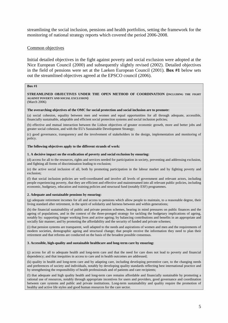
Initial detailed objectives in the fight against poverty and social exclusion were adopted at the Nice European Council (2000) and subsequently slightly revised (2002). Detailed objectives in the field of pensions were set at the Laeken European Council (2001). Box #1 below sets out the streamlined objectives agreed at the EPSCO council (2006). Box #1 STREAMLINED OBJECTIVES UNDER THE OPEN METHOD OF COORDINATION (INCLUDING THE FIGHT

AGAINST POVERTY AND SOCIAL EXCLUSION ) (March 2006) The overarching objectives of the OMC for social protection and social inclusion are to promote:

(a) social cohesion, equality between men and women and equal opportunities for all through adequate, accessible, financially sustainable, adaptable and efficient social protection systems and social inclusion policies;

(b) effective and mutual interaction between the Lisbon objectives of greater economic growth, more and better jobs and greater social cohesion, and with the EU's Sustainable Development Strategy;

(c) good governance, transparency and the involvement of stakeholders in the design, implementation and monitoring of policy. The following objectives apply to the different strands of work: 1. A decisive impact on the eradication of poverty and social exclusion by ensuring:

(d) access for all to the resources, rights and services needed for participation in society, preventing and addressing exclusion, and fighting all forms of discrimination leading to exclusion;

(e) the active social inclusion of all, both by promoting participation in the labour market and by fighting poverty and exclusion;

(f) that social inclusion policies are well-coordinated and involve all levels of government and relevant actors, including people experiencing poverty, that they are efficient and effective and mainstreamed into all relevant public policies, including economic, budgetary, education and training policies and structural fund (notably ESF) programmes. 2. Adequate and sustainable pensions by ensuring:

(g) adequate retirement incomes for all and access to pensions which allow people to maintain, to a reasonable degree, their living standard after retirement, in the spirit of solidarity and fairness between and within generations;

(h) the financial sustainability of public and private pension schemes, bearing in mind pressures on public finances and the ageing of populations, and in the context of the three-pronged strategy for tackling the budgetary implications of ageing, notably by: supporting longer working lives and active ageing; by balancing contributions and benefits in an appropriate and socially fair manner; and by promoting the affordability and the security of funded and private schemes;

(i) that pension systems are transparent, well adapted to the needs and aspirations of women and men and the requirements of modern societies, demographic ageing and structural change; that people receive the information they need to plan their retirement and that reforms are conducted on the basis of the broadest possible consensus. 3. Accessible, high-quality and sustainable healthcare and long-term care by ensuring:

(j) access for all to adequate health and long-term care and that the need for care does not lead to poverty and financial dependency; and that inequities in access to care and in health outcomes are addressed;

(k) quality in health and long-term care and by adapting care, including developing preventive care, to the changing needs and preferences of society and individuals, notably by developing quality standards reflecting best international practice and by strengthening the responsibility of health professionals and of patients and care recipients;

(l) that adequate and high quality health and long-term care remains affordable and financially sustainable by promoting a rational use of resources, notably through appropriate incentives for users and providers, good governance and coordination between care systems and public and private institutions. Long-term sustainability and quality require the promotion of healthy and active life styles and good human resources for the care sector.

6

Common indicators

Initial portfolio (social inclusion) Building on the prior work of Eurostat (Statistical Programming Committee guidelines, 1998) and academic research on behalf of DG Employment and Social Affairs (Atkinson Report #1, 2001), it is within the reporting and monitoring context of the Open Method of Coordination that the Laeken European Council in December 2001 endorsed some best practice criteria for indicator design, and a first set of 18 common statistical indicators for social inclusion which allowed monitoring in a comparable way of Member States’ progress towards the agreed EU objectives. After the Laeken European Council, the Indicators Sub-Group (ISG) continued working with a view to refining and consolidating the original list of indicators. The Social Protection Committee subsequently approved a revised list of commonly agreed indicators in July 2003. Second portfolio (adequacy and sustainability of pensions) Building on the work on social inclusion, and in collaboration with the Employment Committee and Ageing Working Group of the Economic Policy Committee, indicators were also developed for the OMC on pensions. For the second round of strategy reporting, detailed lists were suggested in a note to Member States issued in October 2004. Streamlining Further academic research was commissioned on behalf of the Luxembourgish Presidency (Atkinson Report #2, 2005) and areas for future development were identified. In May 2006, the Social Protection Committee (SPC) endorsed new best practice criteria for indicator design (see Box #2), and adopted proposals for a portfolio of overarching indicators and for streamlining the social inclusion, pensions and health portfolios, to adapt monitoring to reflect the strategic reports for 2006-2008 to be prepared in line with the March 2006 EPSCO council objectives.

7

Box #2 GUIDING PRINCIPLES FOR THE SELECTION OF INDICATORS AND STATISTICS (May 2006) The indicator portfolio:

(1) should be comprehensive and cover all key dimensions of the common objectives;

(2) should be balanced across the different dimensions;

(3) should enable a synthetic and transparent assessment of a country's situation in relation to the common objectives. The selection of individual indicators:

(a) an indicator should capture the essence of the problem and have a clear and accepted normative interpretation;

(b) an indicator should be robust and statistically validated;

(c) an indicator should provide a sufficient level of cross country comparability, as far as practicable with the use of internationally applied definitions and data collection standards;

(d) an indicator should be built on available underlying data, and be timely and susceptible to revision;

(e) an indicator should be responsive to policy interventions but not subject to manipulation. Each strand portfolio will therefore contain:

- Commonly agreed EU indicators contributing to a comparative assessment of MS progress towards the common objectives. These indicators might refer to social outcomes, intermediate social outcomes or outputs.

- Commonly agreed National indicators based on commonly agreed definitions and assumptions that provide key information to assess the progress of MS in relation to certain objectives, while not allowing for a direct cross-country comparison, or not necessarily having a clear normative interpretation. These indicators are especially suited to measure the scale and nature of policy intervention. These indicators should be interpreted jointly with the relevant background information (exact definition, assumptions, representativeness).

- Context information: each portfolio will have to be assessed in the light of key context information, and by referring to past, and where relevant, future trends. The list of context information proposed is indicative and leaves room to other background information that would be most relevant to better frame and understand the national context.

List of Overarching Indicators The list of Overarching Indicators contains 14 headline indicators and 12 context indicators – more if various breakdowns are treated separately. Table #1 contains the agreed definitions from the SPC text, with clarifications added for the context indicators and certain other indicators.

8

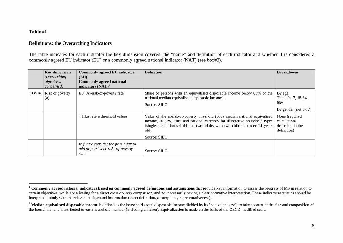
Table #1 Definitions: the Overarching Indicators The table indicates for each indicator the key dimension covered, the “name” and definition of each indicator and whether it is considered a commonly agreed EU indicator (EU) or a commonly agreed national indicator (NAT) (see box#3).

Key dimension

(overarching objectives concerned)

Commonly agreed EU indicator (EU) Commonly agreed national indicators (NAT)1

Definition Breakdowns

OV-1a Risk of poverty (a)

EU: At-risk-of-poverty rate

Share of persons with an equivalised disposable income below 60% of the national median equivalised disposable income2.

Source: SILC

By age: Total, 0-17, 18-64, 65+

By gender (not 0-17)

+ Illustrative threshold values

Value of the at-risk-of-poverty threshold (60% median national equivalised income) in PPS, Euro and national currency for illustrative household types (single person household and two adults with two children under 14 years old)

Source: SILC

None (required calculations described in the definition)

In future consider the possibility to add at-persistent-risk- of-poverty rate

Source: SILC

1 Commonly agreed national indicators based on commonly agreed definitions and assumptions that provide key information to assess the progress of MS in relation to certain objectives, while not allowing for a direct cross-country comparison, and not necessarily having a clear normative interpretation. These indicators/statistics should be interpreted jointly with the relevant background information (exact definition, assumptions, representativeness). 2 Median equivalised disposable income is defined as the household's total disposable income divided by its "equivalent size", to take account of the size and composition of the household, and is attributed to each household member (including children). Equivalization is made on the basis of the OECD modified scale.

9

Key dimension (overarching objectives concerned)



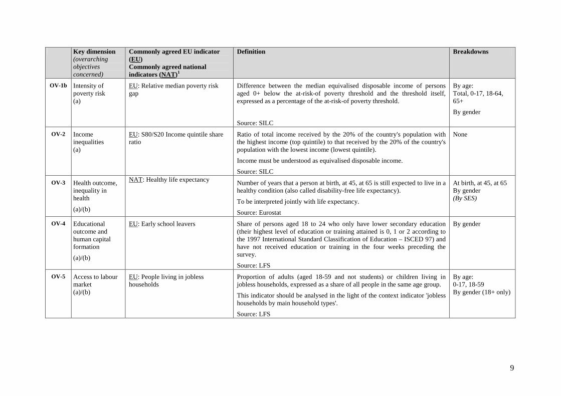
OV-1b Intensity of poverty risk (a)

EU: Relative median poverty risk gap

Difference between the median equivalised disposable income of persons aged 0+ below the at-risk-of poverty threshold and the threshold itself, expressed as a percentage of the at-risk-of poverty threshold.

Source: SILC

By age: Total, 0-17, 18-64, 65+

By gender

OV-2 Income inequalities (a)

EU: S80/S20 Income quintile share ratio

Ratio of total income received by the 20% of the country's population with the highest income (top quintile) to that received by the 20% of the country's population with the lowest income (lowest quintile).

Income must be understood as equivalised disposable income.

Source: SILC

None

OV-3 Health outcome, inequality in health

(a)/(b)

NAT: Healthy life expectancy

Number of years that a person at birth, at 45, at 65 is still expected to live in a healthy condition (also called disability-free life expectancy).

To be interpreted jointly with life expectancy.

Source: Eurostat

At birth, at 45, at 65 By gender (By SES)

OV-4 Educational outcome and human capital formation

(a)/(b)

EU: Early school leavers Share of persons aged 18 to 24 who only have lower secondary education (their highest level of education or training attained is 0, 1 or 2 according to the 1997 International Standard Classification of Education – ISCED 97) and have not received education or training in the four weeks preceding the survey.

Source: LFS

By gender

OV-5 Access to labour market (a)/(b)

EU: People living in jobless households

Proportion of adults (aged 18-59 and not students) or children living in jobless households, expressed as a share of all people in the same age group.

This indicator should be analysed in the light of the context indicator 'jobless households by main household types'.

Source: LFS

By age: 0-17, 18-59 By gender (18+ only)

10




OV-6 Financial Sustainability of social protection systems

(a)

NAT: Projected Total Public Social expenditures

Age-related projections of total public social expenditures (e.g. pensions, health care, long-term care, education and unemployment transfers), current level (% of GDP) and projected change in share of GDP (in percentage points) (2010-2020-2030-2040-2050)

Specific assumptions agreed in the AWG/EPC. See "The 2005 EPC projections of age-related expenditures (2004-2050) for EU-25: underlying assumptions and projection methodologies"

Source: EPC/AWG

None

OV-7a Pensions adequacy (a)

EU: Relative median income of elderly people

The ratio of the median equivalised disposable income of people aged 65+ to income of people aged 0-64.

Source: SILC

None

OV-7b Pensions adequacy (a)

EU: Aggregate replacement ratio Median individual pensions of persons aged 65-74 relative to median individual earnings of persons aged 50-59, excluding other social benefits

Source: SILC

By gender

OV-8 Inequalities in access to health care (a)

EU: Unmet need for care

Source: SILC

None

OV-9 Improved standards of living resulting from economic growth (a)/(b)

EU: At-risk-of-poverty rate anchored at a fixed moment in time (2005)

Possibly replaced or supplemented in the future by material deprivation or consistent poverty indicators

Share of persons aged 0+ with an equivalised disposable income below the at-risk-of-poverty threshold calculated in the base year (1st EU-SILC income reference year for all 25 EU countries), adjusted for inflation over the years.

Source: SILC

By age: Total, 0-17, 18-64, 65+ By gender (18+ only)

11




OV-10 Employment of older workers (a)/(b)

EU: Employment rate of older workers

Possibly replaced or supplemented by "average exit age from the labour market" when quality issues are resolved

Persons in employment in age groups 55-59 and 60–64 as a proportion of total population in the same age group.

Source: LFS

By age: 55-59; 60-64

By gender

OV-11 In-work poverty (a)/(b)

EU: In-work at-risk-of poverty rate Individuals who are classified as employed3 (including “wage and salary employment plus self-employment, etc.) and who are at risk of poverty. This indicator needs to be analysed according to personal, job and household characteristics. It should also be analysed in comparison with the poverty risk faced by the unemployed and the inactive.

Source: SILC

By gender

(only 18+ population is considered for this indicator)

OV-12 Participation in labour market (a)/(b)

EU: Activity rate

Possibly replaced or supplemented in future by MWP indicators

Share of employed and unemployed people in total population of working age 15-64.

Source: LFS

By gender and age: 15-24, 25-54, 55-59; 60-64; Total

OV-13 Regional cohesion (a)/(b)

NAT: Regional disparities – coefficient of variation of employment rates

Standard deviation4 of regional employment rates divided by the weighted national average (age group 15-64 years). (NUTS - nomenclature of territorial units for statistics - II)

Source: LFS

3 Individuals classified as employed according to the definition of most frequent activity status. The most frequent activity status is defined as the status that individuals declare to have occupied for more than half the number of reported months. 4 Standard deviation measures how, on average, the situation in regions differs from the national average. As a complement to the indicator, a graph showing max/min/average per country is presented. Possible alternative measures: Regional disparities – underperforming regions. Source LFS 1. Share of underperforming regions in terms of employment and unemployment (in relation to all regions and to the working age population/labour force) (NUTS II). 2. Differential between average employment/unemployment of the underperforming regions and the national average in relation to the national average of employment/unemployment (NUTS II). Thresholds to be applied: 90% and 150% of the national average rate for employment and unemployment, respectively. (An extra column with the national employment and unemployment rates would be included)

12




OV-14 More health (a)/(b)

To be decided following ISG work on health indicators

Definitions: the context indicators




OV-1 GDP growth Growth rate of GDP volume - percentage change on previous year

Source: STRIND

OV-2 Employment rate The employment rate is calculated by dividing the number of persons aged 15 to 64 in employment by the total population of the same age group.

Source: LFS

By gender

Unemployment rate Unemployment rates represent unemployed persons as a percentage of the labour force. The labour force is the total number of people employed and unemployed. Unemployed persons comprise persons aged 15+ who were: a. without work during the reference week, b. currently available for work, i.e. were available for paid employment or self-employment before the end of the two weeks following the reference week, c. actively seeking work, i.e. had taken specific steps in the four weeks period ending with the reference week to seek paid employment or self-employment or who found a job to start later, i.e. within a period of, at most, three months.

Source: LFS

By key age groups:

By gender

5 Commonly agreed national indicators based on commonly agreed definitions and assumptions that provide key information to assess the progress of MS in relation to certain objectives, while not allowing for a direct cross-country comparison, and not necessarily having a clear normative interpretation. These indicators/statistics should be interpreted jointly with the relevant background information (exact definition, assumptions, representativeness).

13




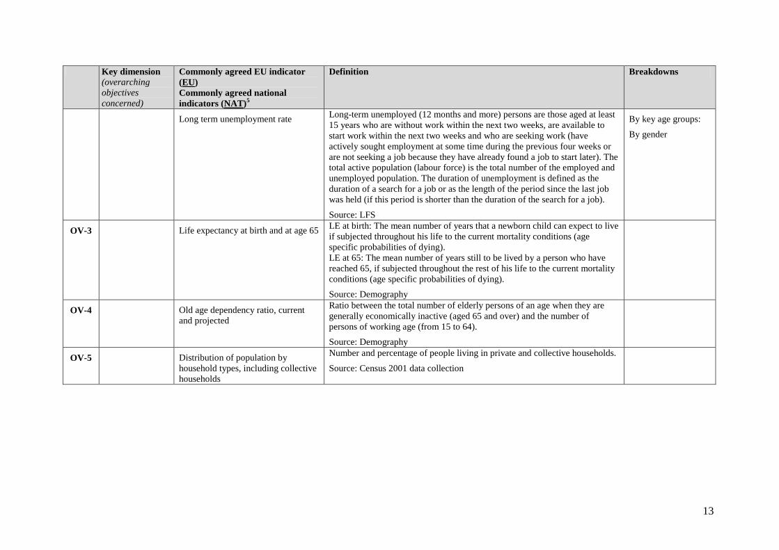
Long term unemployment rate Long-term unemployed (12 months and more) persons are those aged at least 15 years who are without work within the next two weeks, are available to start work within the next two weeks and who are seeking work (have actively sought employment at some time during the previous four weeks or are not seeking a job because they have already found a job to start later). The total active population (labour force) is the total number of the employed and unemployed population. The duration of unemployment is defined as the duration of a search for a job or as the length of the period since the last job was held (if this period is shorter than the duration of the search for a job).

Source: LFS

By key age groups:

By gender

OV-3 Life expectancy at birth and at age 65 LE at birth: The mean number of years that a newborn child can expect to live if subjected throughout his life to the current mortality conditions (age specific probabilities of dying). LE at 65: The mean number of years still to be lived by a person who have reached 65, if subjected throughout the rest of his life to the current mortality conditions (age specific probabilities of dying).

Source: Demography

OV-4 Old age dependency ratio, current and projected

Ratio between the total number of elderly persons of an age when they are generally economically inactive (aged 65 and over) and the number of persons of working age (from 15 to 64).

Source: Demography

OV-5 Distribution of population by household types, including collective households

Number and percentage of people living in private and collective households.

Source: Census 2001 data collection

14




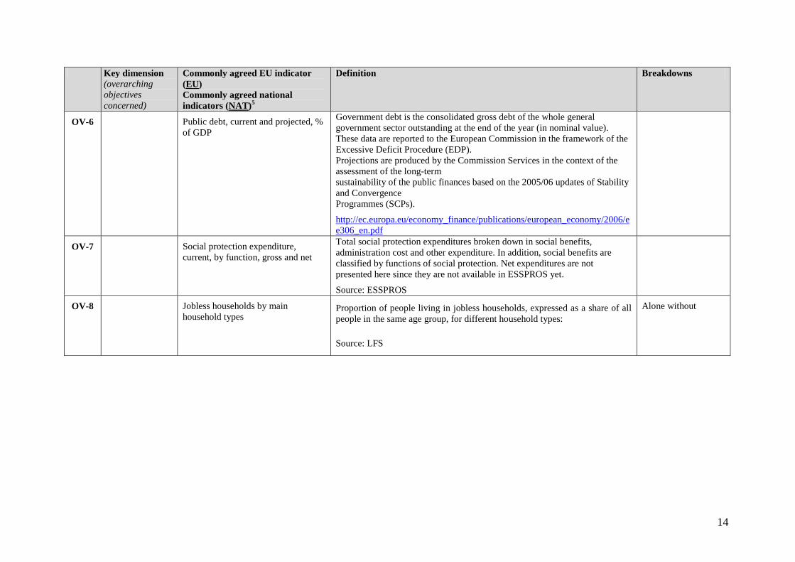
OV-6 Public debt, current and projected, % of GDP

Government debt is the consolidated gross debt of the whole general government sector outstanding at the end of the year (in nominal value). These data are reported to the European Commission in the framework of the Excessive Deficit Procedure (EDP). Projections are produced by the Commission Services in the context of the assessment of the long-term sustainability of the public finances based on the 2005/06 updates of Stability and Convergence Programmes (SCPs).

http://ec.europa.eu/economy_finance/publications/european_economy/2006/ee306_en.pdf

OV-7 Social protection expenditure, current, by function, gross and net

Total social protection expenditures broken down in social benefits, administration cost and other expenditure. In addition, social benefits are classified by functions of social protection. Net expenditures are not presented here since they are not available in ESSPROS yet.

Source: ESSPROS

OV-8 Jobless households by main household types

Proportion of people living in jobless households, expressed as a share of all people in the same age group, for different household types:

Source: LFS

Alone without

15




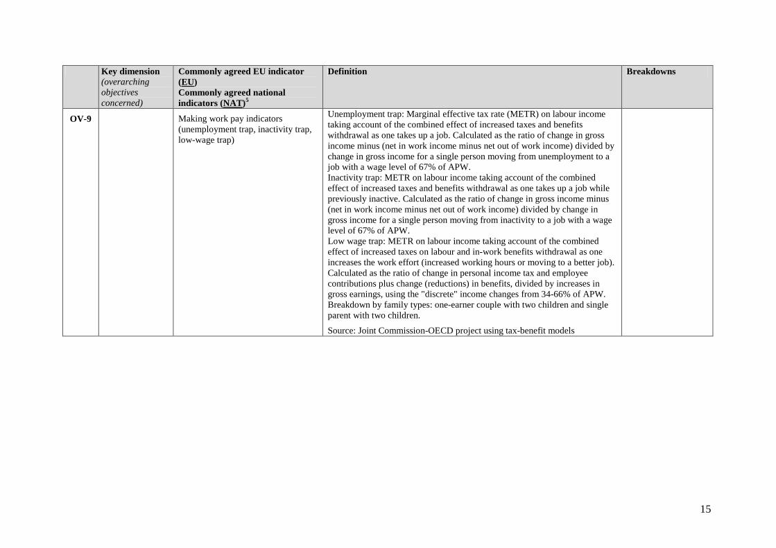
OV-9 Making work pay indicators (unemployment trap, inactivity trap, low-wage trap)

Unemployment trap: Marginal effective tax rate (METR) on labour income taking account of the combined effect of increased taxes and benefits withdrawal as one takes up a job. Calculated as the ratio of change in gross income minus (net in work income minus net out of work income) divided by change in gross income for a single person moving from unemployment to a job with a wage level of 67% of APW. Inactivity trap: METR on labour income taking account of the combined effect of increased taxes and benefits withdrawal as one takes up a job while previously inactive. Calculated as the ratio of change in gross income minus (net in work income minus net out of work income) divided by change in gross income for a single person moving from inactivity to a job with a wage level of 67% of APW. Low wage trap: METR on labour income taking account of the combined effect of increased taxes on labour and in-work benefits withdrawal as one increases the work effort (increased working hours or moving to a better job). Calculated as the ratio of change in personal income tax and employee contributions plus change (reductions) in benefits, divided by increases in gross earnings, using the "discrete" income changes from 34-66% of APW. Breakdown by family types: one-earner couple with two children and single parent with two children.

Source: Joint Commission-OECD project using tax-benefit models

16




OV-10 Net income of social assistance recipients as a % of the at-risk-of-poverty threshold

This indicator refers to the income of people living in households that only rely on "last resort" social assistance benefits (including related housing benefits) and for which no other income stream is available (from other social protection benefits – e.g. unemployment or disability schemes – or from work). The aim of such an indicator is to evaluate if the safety nets provided to those households most excluded from the labour market are sufficient to lift people out of poverty. This indicator is calculated on the basis of the tax-benefit models developed jointly by the OECD and the European Commission. It is only calculated for Countries where non-categorical social benefits are in place and for 3 jobless household types: single person, lone parent, 2 children and couple with 2 children. This indicator is especially relevant when analysing MWP (Making work pay) indicators.

Source: Joint EC-OECD project using OECD tax-benefit models, and Eurostat.

OV-11 EU: At-risk-of-poverty rate before social transfers (other than pensions)

Relative at-risk-of-poverty rate where equivalised income is calculated including retirement and survivors' pensions and excluding all other social transfers.

Source: SILC

Age groups: Total, 0-17; 18-64; 65+

17




OV-12 NAT: change in projected theoretical replacement ratio for base case 2004-2050 accompanied with information on type of pension scheme [DB (defined benefit), DC (defined contribution), NDC (notional defined contribution)] and

NAT: change in projected theoretical replacement ratio for base case 2004-2050 accompanied with information on type of pension scheme (DB, DC, NDC) and change in projected public pension expenditure 2004-2050

Change in the theoretical level of income from pensions at the moment of take-up related to the income from work in the last year before retirement for a hypothetical worker (base case), percentage points, 2004-2050, with information on the type of pension scheme (DB, DC or NDC) and changes in the public pension expenditure as a share of GDP, 2004-2050. This information can only collectively form the indicator called projected theoretical replacement ratio. Results relate to current and projected, gross (public and private) and total net replacement rates, and should be accompanied by information on representativeness and assumptions (contribution rates and coverage rate, public and private), and calculations of changes in replacement rates for 1 or 2 other cases, if suitable (e.g. OECD). Specific assumptions agreed in the ISG. For further details, see 2006 report on Replacement Rates. http://ec.europa.eu/employment_social/social_protection/docs/isg_repl_rates_en.pdf

Source: ISG and AWG

18

Reporting and monitoring

A first combined Joint Report on Social Protection and Social Inclusion was published in 2005, together with a set of summary country-by-country fiches. Underpinning the preparation of the overarching report, the Commission services continued publishing separate and more in-depth reports focusing on the underlying National Action Plans and a detailed Statistical Annex (http://ec.europa.eu/employment_social/social_inclusion/naps_en.htm). The first national strategy reports under the streamlined objectives apply for 2006-2008.

Common data sources

In order to maximise the cross-country comparability of the common indicators, in addition to defining their calculation algorithms, common harmonised data sources are necessary. The EU Labour Force Survey (LFS) has been explicitly recognised as the data source for the construction of all the employment-related commonly agreed indicators. A detailed description of this survey and the definitions used is presented in the Eurostat publications “Labour Force Survey – Methods and definitions, 2001” and “Labour Force Survey in Central and Eastern European countries – Methods and definitions, 2000” both published by the European Commission. When the Open Method of Coordination was launched, many income-based and other indicators were initially specified to be calculated on the basis of the European Community Household Panel (ECHP). However, this pioneering survey only covered the EU15 member states and expired in 2001. It has been replaced by data collection under the Community Statistics on Income and Living Conditions (SILC) framework regulation (EC no.1177/2003 of 16th June 2003) and its associated implementing regulations. A list of the relevant regulations issued to date and their references in the Official Journal is included as an appendix (see Appendix I). SILC is considered as the EU reference source for income and social exclusion statistics, and for the commonly agreed indicators of social cohesion in particular. SILC was launched in 2003 for six member states, coverage expanded to fifteen countries in 2004, and with effect from 2005 it covers 25 EU Member States together with Iceland and Norway. Bulgaria, Romania, Turkey and Switzerland have launched SILC in 2006. There are plans to expand coverage to other countries. Details concerning SILC can be found at the following address: http://epp.eurostat.ec.europa.eu/portal/page/portal/living_conditions_and_social_protection/introduction/income_social_inclusion_living_conditions During the transition between ECHP and SILC, indicators have been/are compiled by Eurostat on the basis of national sources. A table of the alternatives sources used is included in Appendix II . Whilst every effort has been made to maximise the consistency of

19

definitions and concepts, the resulting indicators cannot be considered to be fully comparable to the SILC based indicators.

Some limitations of the indicators due to the data sources

EU-SILC concepts and definitions keep as closely as possible to the international recommendations of the UN 'Canberra Manual'. Typically, coverage of the SILC and national data sources is restricted to private households and excludes persons living in institutions. Certain hard-to-reach groups of the population such as persons who are homeless or nomadic are also de facto not covered. The exclusions may distort comparisons between countries where certain traditions favour caring for vulnerable people within their families, whilst others favour institutional care arrangements. Whilst it is considered to be the best basis for poverty and social exclusion analysis (for example it avoids the moral hazard of actual expenditure choices), income is acknowledged to be an imperfect measure of welfare and consumption capabilities. Amongst other things it does not reflect access to credit, access to accumulated savings or ability to liquidate accumulated assets, informal community support arrangements, aspects of non-monetary deprivation, differential pricing and other aspects. These factors may be of particular relevance for persons at the lower extreme of the income distribution. The bottom 10 per cent of the income distribution should not, therefore, necessarily be interpreted as having the bottom 10 per cent of living standards.

Income definition

In SILC, the household total disposable income is taken to be all net monetary income received by the household and its members during the income reference year – namely all income from work (employee wages and self-employment earnings), private income from investment and property6, transfers between households plus all social transfers received in cash including old-age pensions, net of any taxes and social contributions paid. No account is taken of in kind social transfers. Until 2007, no account had to be taken of income-in-kind (with the exception of company car) and imputed rent (i.e. the money that one saves on full (market) rent by living in one’s own accommodation or in accommodation rented at a price that is lower than the market rent), mortgage loan interest payments, etc. Although certain countries (e.g. DK) are already able to supply income figures including imputed rent, until this becomes mandatory for all countries (2007 data), for reasons of comparability, the income definition underlying the calculation of indicators currently excludes imputed rent. This could have a distorting effect in comparisons between countries, or between population sub-groups, when the distribution of accommodation tenure status varies. This impact may be particularly apparent for the elderly who may have been able to accumulate wealth in the form of housing assets.

6 In accordance with a recent decision of the SILC methodological task force, regular income from private pension plans will be taken into account from the 2007 data collection onwards.

20

For the twelve new EU member countries as well as Turkey, income-in-kind is considered to be a more widespread and more substantial component of household disposable income than for EU15 Member States and EFTA countries. ‘Income-in-kind’ describes the value of goods produced directly by the household through either a private or a professional activity and consumed by them (or donated to others). Some income-in-kind is covered in SILC (e.g. the variable PY070 covers own production of food by households). By contrast other items are not included in SILC (e.g. value of services provided by self-employed persons free of charge to members of their own household or to others, own production of non-food products like wood). Since 2003, the use of company vehicles is included in the SILC definition (variable PY020). From the 2007 data collection, this variable will also collect a range of other services obtained free of charge by employees as part of a professional activity. These are then also classified as ‘non-cash employee income’ with effect from the 2007 data collection (e.g. accommodation provided free or at reduced rent by the employer, free or subsidised meals at work, crèche facilities for young children, school fees of older children, subsidised loans, other goods and services provided free or at reduced price). Income from the rental of property or land which is received in kind rather than in cash should be valued and treated as imputed rent (SILC variable HY030). It is worth emphasising that collecting information regarding ‘income-in-kind’ involves overcoming a number of practical difficulties, due to the different methods of identifying it and estimating ‘income-in-kind’ values, and due to the different relative importance of this income in the different countries (and different population groups within countries). However, a harmonisation process is in progress. A key objective of SILC is to deliver robust and comparable data on total disposable household income, total disposable household income before transfers (other than old-age and survivors' benefits; including old-age and survivors' benefits), total gross income and gross income at component level. A derogation has been granted to and used by Greece, Spain, France, Italy and Portugal not to deliver any gross income data as from the first year of launching SILC. These countries will, deliver these data from the 2007 data collection onwards at the latest. Where these countries are unable to deliver a gross income data component, the corresponding net income component is required instead. Where national sources are used, there is an attempt to approximate as closely as possible to the SILC income concept by performing some adjustments to the standard information collected from national sources. The impact of these on reported values can sometimes be significant. Given the sensitivity of the topics covered by the different sources, care is needed when interpreting results; in particular, trends obtained by combining two different sources should be regarded as unreliable. Comparability of income data obtained directly from interviewed individuals with income data obtained from administrative sources is debatable. Care should be taken when analysing information on income at the two extremes of the income distribution. It is also the case for certain components of income, namely income from self-employment, capital income or income from the hidden economy. It is universally acknowledged that self-employment income is one of the most problematic

21

elements of household income to define and measure accurately. Moreover, there is evidence that self-employment is becoming more prevalent in the EU and more heterogeneous in nature.

Equivalisation

Household income is equivalised (adjusted) in order to reflect differences in household size and composition. The equivalised income is then given per equivalent adult. In other words, the total household income is divided by its equivalent size using the so-called “modified OECD” equivalence scale. This equivalence scale gives a weight of 1.0 to the first adult, 0.5 to any other household member aged 14 and over and 0.3 to each child aged less than 14. The resulting figure is attributed to each member of the household, whether adult or children. The equivalent size of a household that consists of 2 adults and 2 children below the age of 14 is therefore: 1.0 + 0.5 + (2 0.3) = 2.1⋅

Income reference period

Surveys can have different income reference periods (e.g. monthly vs. yearly, last 12 months vs. previous calendar year, etc.), which may have an impact on the reported values and their comparability between countries. In SILC, the reference period for collecting income is a year. However, the income variable may not be fully comparable between sub-samples when the survey is conducted at different periods of the year (i.e. in continuous surveys for which the income reference period is the last twelve months or the current year in case current income is annualised). In this case, if the above mentioned facts are not taken into account, the income distribution (and the results in terms of poverty risk) can be biased by the variability of seasonal income components (such as income from agriculture, self-employment, thirteenth and fourteenth month payment). The remark goes particularly for the Household Budget Survey for which the period of collecting income varies over the year. Prior to the launch of SILC, the income reference period of the national sources used was the same as the survey year for the national data sources in Estonia, Cyprus, Latvia, Lithuania, Hungary, Malta, Netherlands, Poland, Slovenia and Sweden. For ECHP participant countries it was the preceding year. During the transition period, the relevant data for Czech Republic, Cyprus, Malta and Slovakia was drawn from periodic sources rather than annual sources.

EU averages

In line with policy needs under the Open Method of Coordination, statistics have typically focused on the situation of individuals within each member state, relative to the prevailing situation in that country. However, there is a wide public interest in some sort of common reference against which national figures should be compared, and an aggregate figure for the European Union as a whole.

22

Different approaches for calculating aggregates are possible, including: • Summing the base information for all participant countries and proceeding as if they

relate to a single entity for the calculation of indicators. • Computing indicators separately for participant countries and calculating an average

value. This raises practical questions about what measure of central tendency to adopt and whether weightings should be used (and if so, whether they should be the same for all sub-populations and breakdowns).

• Computing indicators separately for participant countries, but applying a common reference threshold, where applicable.

In line with 1998 Statistical Programming Committee guidelines, prior to the availability of SILC microdata for a majority of countries, group-of-country averages were calculated as population-weighted averages of the available national values, with a single value (the official total population value for the number of persons living in private households) being applied to weight all the calculations: indicators are not presented for any given year when data is not available for countries representing 25% or more of the population of the group concerned. This approach has the merit of simplicity and transparency. However, there is a clear risk that population sub groups within each country do not follow a standard proportion across any given group – with consequent implications for the information value of an indicator assuming such a standard proportion did apply. With the availability of SILC microdata, a more refined approach is possible: each indicator can be weighted using the specific weights for the population group concerned.

Weighting scheme for the calculation of EU averages

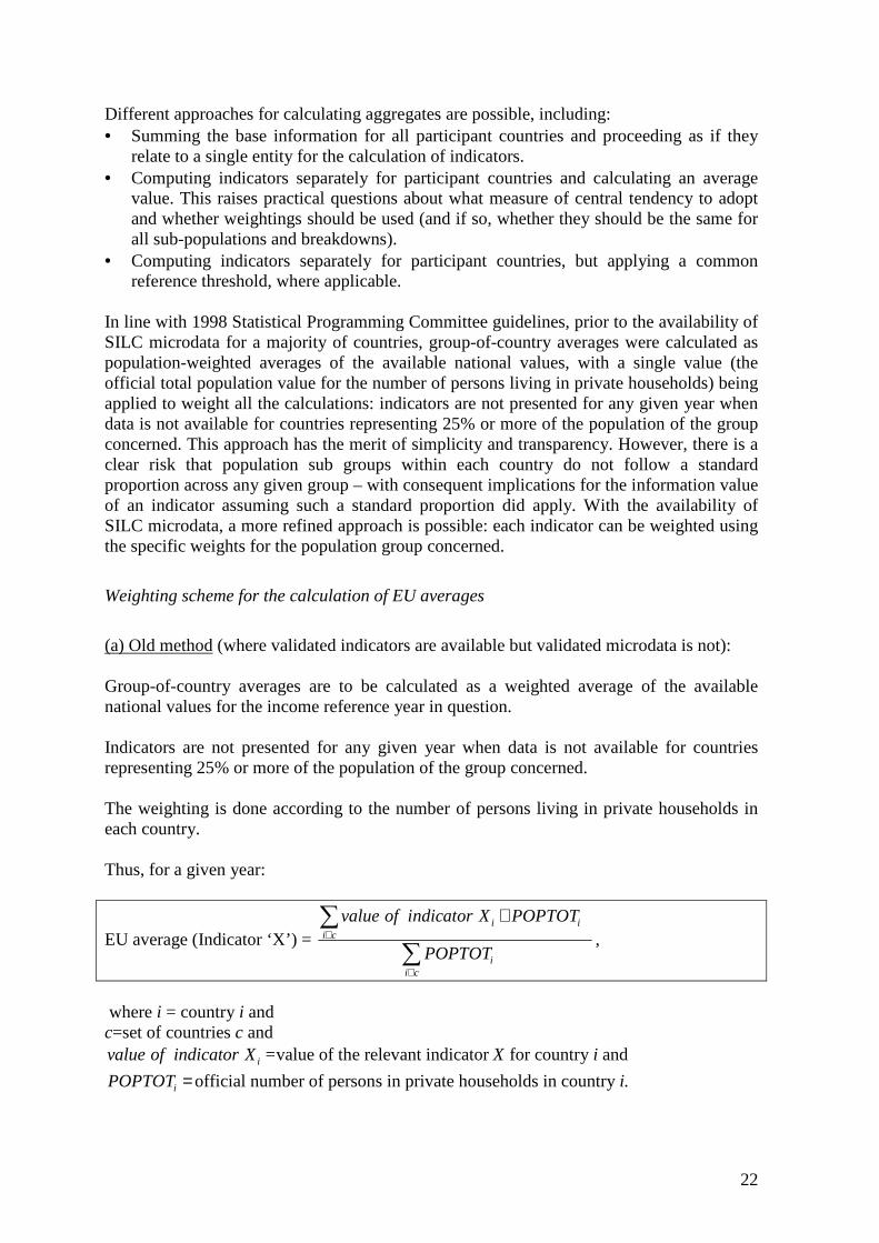
(a) Old method (where validated indicators are available but validated microdata is not): Group-of-country averages are to be calculated as a weighted average of the available national values for the income reference year in question. Indicators are not presented for any given year when data is not available for countries representing 25% or more of the population of the group concerned. The weighting is done according to the number of persons living in private households in each country. Thus, for a given year:

EU average (Indicator ‘X’) = i i

i c

ii c

value of indicator X POPTOT

POPTOT∈

∈

⋅∑

∑,

where i = country i and c=set of countries c and

ivalue of indicator X=value of the relevant indicatorX for country i and

iPOPTOT= official number of persons in private households in country i.

23

Note: Official annual average population estimates (number of persons living in private households) can be found on the Eurostat ‘free data’ website (http://epp.eurostat.ec.europa.eu). (b) Currently implemented method (where validated SILC microdata are available): EU average for proportion on population subgroups If the relevant indicator can be expressed as a proportion of the total subset of interest in each country, then the EU average can be calculated as a weighted average of the value of the indicator in each country i. Note on cross-sectional weights: SILC microdata contains four different types of cross-sectional weights:

• Household cross-sectional weights (target variable DB090), useful to draw inference on the population of private households at national and European levels;

• Personal cross-sectional weights for household members of all ages (target variable RB050), useful to draw inferences on the population of all individuals living in private households;

• Personal cross-sectional weights for household members aged 16 and over (target variable PB040), useful to draw inferences on variables included in the personal questionnaire, for the population of individuals aged 16 and over living in private households;

• Personal cross-sectional weights for selected respondents (target variable PB060), useful to draw inferences about certain variables in countries where a sample of persons is used for non-income questions but income data is collected from registers, for the population of individuals aged 16 and over living in private households.

Most indicators will use the personal cross-sectional weight (RB050) because poverty status is determined at household level and assigned at individual level. The target group concerned is the whole population living in private households. However, for indicators focusing on the population aged 16+ (e.g. in work at-risk-of-poverty rate) the appropriate weight would be the SILC variable PB040. The target variable DB090 is not used for indicators, as those are computed at individual level. The target variable PB060 is not used either as it is only relevant for selected respondents. In Eurostat programmes, in order to ensure the correct representativeness of the different subgroups in the weights are corrected by applying a scaling factor to RB050 obtained as the ratio of the sum of RB050 on all cases and the sum of RB050 on valid (non missing) cases. This procedure can be generalised to take into account some stratification (homogeneous missing group). A similar approach is taken for PB040. Thus:

EU average (Indicator 'X')

i ii c

ii c

value of indicator X POPB

POPB∈

∈

=⋅∑

∑,

24

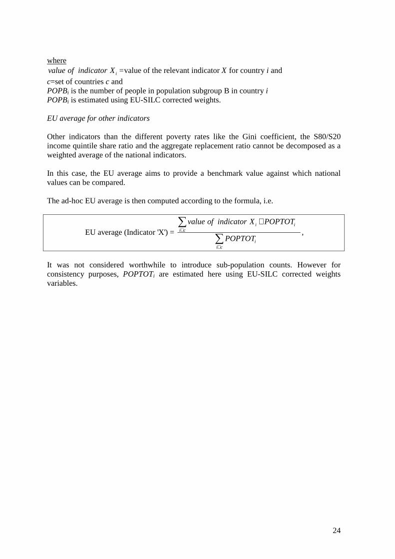
where

ivalue of indicator X=value of the relevant indicatorX for country i and

c=set of countries c and POPBi is the number of people in population subgroup B in country i POPBi is estimated using EU-SILC corrected weights. EU average for other indicators Other indicators than the different poverty rates like the Gini coefficient, the S80/S20 income quintile share ratio and the aggregate replacement ratio cannot be decomposed as a weighted average of the national indicators. In this case, the EU average aims to provide a benchmark value against which national values can be compared. The ad-hoc EU average is then computed according to the formula, i.e.

EU average (Indicator 'X') =

i ii c

ii c

value of indicator X POPTOT

POPTOT∈

∈

⋅∑

∑,

It was not considered worthwhile to introduce sub-population counts. However for consistency purposes, POPTOTi are estimated here using EU-SILC corrected weights variables.

25

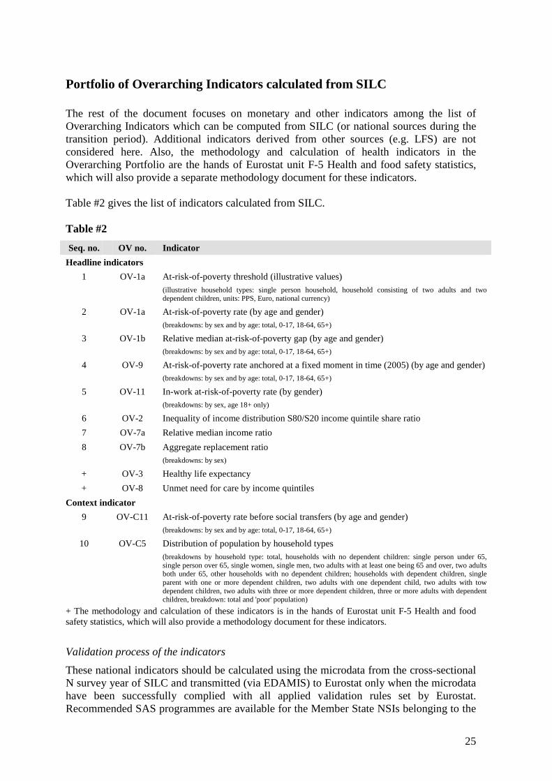
Portfolio of Overarching Indicators calculated from SILC The rest of the document focuses on monetary and other indicators among the list of Overarching Indicators which can be computed from SILC (or national sources during the transition period). Additional indicators derived from other sources (e.g. LFS) are not considered here. Also, the methodology and calculation of health indicators in the Overarching Portfolio are the hands of Eurostat unit F-5 Health and food safety statistics, which will also provide a separate methodology document for these indicators. Table #2 gives the list of indicators calculated from SILC. Table #2

Seq. no. OV no. Indicator

Headline indicators

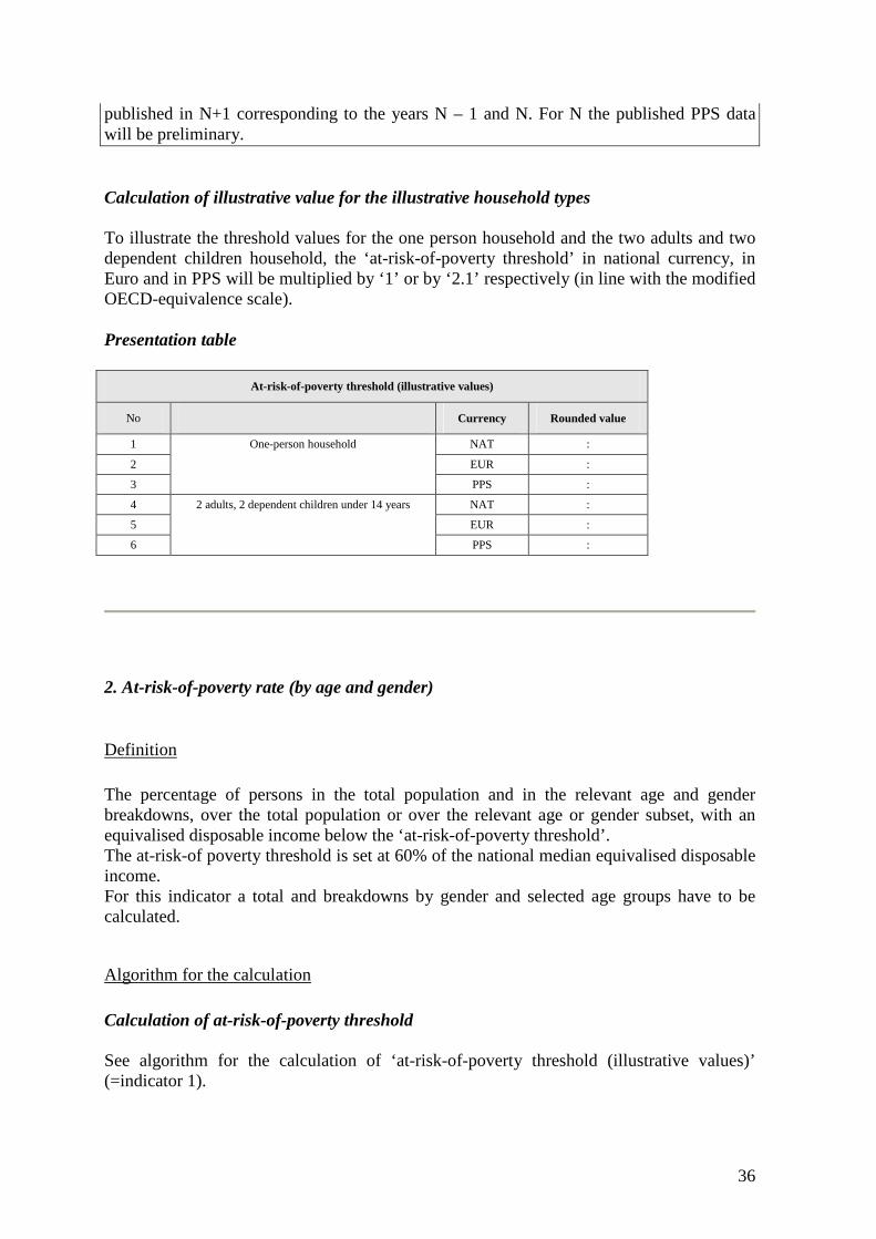
1 OV-1a At-risk-of-poverty threshold (illustrative values) (illustrative household types: single person household, household consisting of two adults and two dependent children, units: PPS, Euro, national currency)

2 OV-1a At-risk-of-poverty rate (by age and gender) (breakdowns: by sex and by age: total, 0-17, 18-64, 65+)

3 OV-1b Relative median at-risk-of-poverty gap (by age and gender) (breakdowns: by sex and by age: total, 0-17, 18-64, 65+)

4 OV-9 At-risk-of-poverty rate anchored at a fixed moment in time (2005) (by age and gender) (breakdowns: by sex and by age: total, 0-17, 18-64, 65+)

5 OV-11 In-work at-risk-of-poverty rate (by gender) (breakdowns: by sex, age 18+ only)

6 OV-2 Inequality of income distribution S80/S20 income quintile share ratio

7 OV-7a Relative median income ratio

8 OV-7b Aggregate replacement ratio (breakdowns: by sex)

+ OV-3 Healthy life expectancy

+ OV-8 Unmet need for care by income quintiles

Context indicator

9 OV-C11 At-risk-of-poverty rate before social transfers (by age and gender) (breakdowns: by sex and by age: total, 0-17, 18-64, 65+)

10 OV-C5 Distribution of population by household types (breakdowns by household type: total, households with no dependent children: single person under 65, single person over 65, single women, single men, two adults with at least one being 65 and over, two adults both under 65, other households with no dependent children; households with dependent children, single parent with one or more dependent children, two adults with one dependent child, two adults with tow dependent children, two adults with three or more dependent children, three or more adults with dependent children, breakdown: total and 'poor' population)

+ The methodology and calculation of these indicators is in the hands of Eurostat unit F-5 Health and food safety statistics, which will also provide a methodology document for these indicators.

Validation process of the indicators

These national indicators should be calculated using the microdata from the cross-sectional N survey year of SILC and transmitted (via EDAMIS) to Eurostat only when the microdata have been successfully complied with all applied validation rules set by Eurostat. Recommended SAS programmes are available for the Member State NSIs belonging to the

26

EU-SILC group on CIRCA. The present document will act as a guiding rule in order to allow Member States to design their own calculations in accordance with the official recommendations. Eurostat will work in parallel to calculate and compare both sets of derived results. When full consistency is achieved, the whole set of indicators (overarching, pension and social exclusion) will be computed by Eurostat. Plausibility will be dealt with during the second phase based on comparisons over time and exogenous (external) information available to Eurostat. Before indicators are released, multilateral validations will be performed. Target dates for the reception of verified/ finalised data by Eurostat will vary from country to country, but anticipated date for the dissemination of indicators for multilateral validation is mid-December of the year N+1.

Publications and income reference year

Publications for dissemination to be prepared during the year N+2 using the Overarching Indicators will include: Joint Report on Social Inclusion and Social Protection; Structural Indicators (“shortlist” and “social cohesion” theme); Sustainable Development Indicators (“poverty” theme and "ageing" theme); the Treaty-based Social Situation in the European Union Report and Eurostat's Yearbook. For the above mentioned publications, indicators relating to survey year N are to be used. Indicators on social exclusion will be labelled using the survey year N as reference. Despite the fact that income refers in most cases to the year N-1, theincoem is collected under the assumption that it is the best available proxy for the living standard at the time of interview (year N). Differences in income reference years are generally pointed out in footnotes.

Publication rules

The standard SILC publication rules will be applied. The minimum precision requirement concerning publication of data collected shall be expressed in terms of number of sample observations on which statistics is based and the level of item non-response (additional to total non-response at unit level). This is set down in the Regulation and is used for publication of data on New Cronos.

• An estimate should not be published if it is based on fewer than 20 sample observations or if the non-response for the item concerned exceeds 50%.

• An estimate should be published with a flag if it is based on 20 to 49 sample observations or if non-response for the item concerned exceeds 20% and is lower or equal to 50%.

• An estimate shall be published in the normal way when based on 50 or more sample observations and the item's non-response does not exceed 20%.

27

The following flags will be used: i see explanatory text (metadata in New Cronos) b break in series (i.e. change of source or change of methodology from that

used in preceding year) s Eurostat estimate u unreliable (i.e. due to small sample size) p provisional

28

Detailed methodological notes

Calculation of age In the EU-SILC regulations, age is defined as the age calculated at the end of the income reference period. However, data collection often occurs a few months after the end of the income reference period, so household composition is captured at the time of interview. Consequently, household members who have died between the end of the income reference period and the time of the survey data collection are not registered and babies born in this interval will be recorded with negative age if age at the end of the income reference period is reconstructed. If the age to be used in analysis and indicator calculation is to be the age at the end of the income reference period, some practical problems are to be solved for the calculation of equivalised household size and indicators. In this case, it is suggested to

• Include these newborn babies in the lowest age group (by setting age to 0) for the calculation of equivalised household size.

• Include such persons for the calculation of indicators for the total population and for the appropriate age breakdowns.

• Include such persons for the calculation of dependent children. In the future, the use of age at the time of interview in analysis will be considered. Indeed the structure of the population is probably better captured at the time of the interview. As long the gap between income collection and recording of household status is not too wide, it is expected that the inconsistency in socio economic analysis will remain minor. On the contrary, it is expected to obtain better coherence between treatment of age and the socio economic situation. This reasoning is not valid when income distribution/ information in relation with age (as for instance, the aggregate replacement ratio or people aged 16) is considered. Potentially relevant SILC variables are DB010 (year of the survey – in D-file), RB010 (year of the survey), RB080 (year of birth), RB070 (month of birth), HB050 (month of household interview), HB060 (year of household interview), PB100 (month of the personal interview), PB110 (year of the personal interview). SILC does not collect the actual date of birth. The month of interview and the month of birth is taken into account when calculating the age. If either is missing, the relevant variables are set to the middle of the year (6): If RB070_F=-1 then RB070=6 If HB050_F=-1 then HB050=6 If the year of birth is missing, age is considered to be missing: If RB080_F=-1 then age=missing (a) For SILC countries where the income reference period is the previous calendar year:

29

• ( ) ( )(DB010 1) 100 12 RB080 100 RB070

AGE = 100

− ⋅ + − ⋅ +

Note: if RB080=DB010, then AGE=-1. (b) For SILC countries where the income reference period is not the previous calendar year:

• ( ) ( )irp_yyyy 100 irp_mm RB080 100 RB070

AGE = 100

⋅ + − ⋅ +

(where irp_yyyy=year of end of income reference period and irp_mm=month of end of income reference period).

Treatment of babies born after the end of the income reference period: Where the income reference period is (a) or (b), babies born after the income reference period will be assigned AGE=-1 by the algorithm describe above. For the calculation of equivalised household size and for the calculation of the indicators if AGE=-1 age is set to AGE=0, i.e. they are included in all calculations. (c) For SILC countries where the income reference period changes:

• ( ) ( )HB060 100 HB050 RB080 100 RB070

AGE = 100

⋅ + − ⋅ +

For all three types of calculations the AGE variable will be truncated before the first decimal point after the operation described above has been performed.

Equivalised disposable income

Definition

For each person, equivalised disposable income (EQ_INCi) is defined as the household's total disposable income divided by its "equivalent size", to take account of the size and composition of the household, and is attributed to each household member. Notes: • The total disposable income of a household is calculated by adding together the personal income received

by all of household members plus income received at household level. • The equivalised household size is defined according to the modified OECD scale (which gives a weight

of 1.0 to the first adult, 0.5 to other household members aged 14 or over and 0.3 to household members aged less than 14).

30

Algorithm for the calculation of disposable income

Calculation of total disposable income To ensure maximum comparability with the detailed definitions adopted in EU-SILC (Commission Regulation No 1980/2003), the total disposable household income should be computed as follows: name SILC-Reference total disposable household income corrected for individual non response

HY020 HY0257

total disposable household income recorded HY020 = the sum for all household members of gross personal income components: gross cash or near-cash employee income; PY010G + gross non-cash employee income; PY020G + employers' social insurance contributions8; PY030G + gross cash profits or losses from self-employment (including

royalties); PY050G

+ value of goods produced for own consumption9; PY070G + unemployment benefits; PY090G + old-age benefits; PY100G + survivors' benefits; PY110G + sickness benefits; PY120G + disability benefits PY130G + education-related allowances PY140G gross income components at household level: + income from rental of a property or land; HY040G + imputed rent; HY030G + family/children-related allowances; HY050G + social exclusion not elsewhere classified; HY060G + housing allowances; HY070G + regular inter-household cash transfers received; HY080G + interests, dividends, profit from capital investments in

unincorporated business; HY090G

+ income received by people aged under 16; HY110G deductions: − employers' social insurance contributions; PY030G − mortgage interest; HY100G − regular taxes on wealth; HY120G − regular inter-household cash transfer paid; HY130G − tax on income and social insurance contributions.

(The variable the ‘tax on income and social insurance contributions’ includes tax adjustments-repayment/receipt on income, income tax at source and social insurance

HY140G

7 Until 2006, the recommendation is to collect the recorded total disposable income in HY020. From 2007, following a new recommendation concerning treatment of missing individuals, it was decided to gather the estimated value of the total disposable income corrected for individual non response in HY020. 8 According to Canberra recommendations, employers' social contributions are to be included in the gross calculation 9 Income components, which are mandatory from 2007 onwards only are included in italics.

31

contributions (if applicable).)

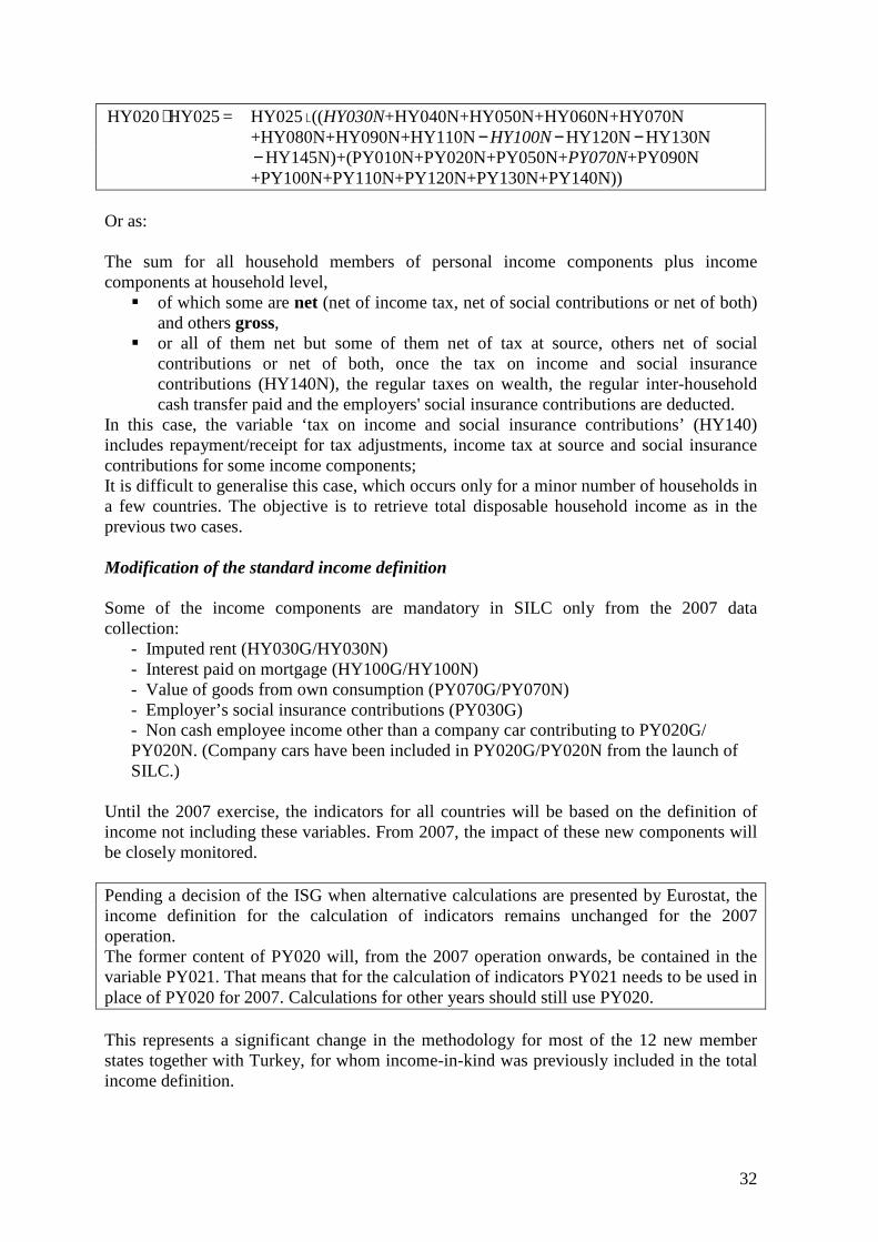
All multiplied by � within-household non-response inflation factor HY025 HY020 HY025⋅ = HY025⋅ ((HY030G+HY040G+HY050G+HY060G+HY070G+HY080G

+HY090G+HY110G− HY100G− HY120G− HY130G− HY140G) +(PY010G+PY020G+PY030G+PY050G+PY070G+PY090G+PY100G +PY110G+PY120G+PY130G+PY140G− PY030G))

Or equivalently (for net income data collection) name SILC-Reference total disposable household income corrected for individual non response

HY020 HY025

total disposable household income HY020 = the sum for all household members of net (of income tax at source and of social contributions) personal income components: cash or near-cash employee income; PY010N + non-cash employee income; PY020N + cash profits or losses from self-employment; PY050N + value of goods produced for own consumption; PY070N + unemployment benefits; PY090N + old-age benefits; PY100N + survivors' benefits; PY110N + sickness benefits; PY120N + disability benefits; PY130N + education-related allowances; PY140N net (of income tax at source and of social contributions) income components at household level: + income from rental of a property or land; HY040N + imputed rent; HY030N + family/children-related allowances; HY050N + social exclusion not elsewhere classified; HY060N + housing allowances; HY070N + inter-household cash transfers received; HY080N + interests, dividends, profit from capital investments in

unincorporated business; HY090N

+ income received by people aged under 16; HY110N deductions − mortgage interest HY100N − regular taxes on wealth HY120N − regular inter-household cash transfer paid HY130N − repayment/receipt for tax adjustments on income HY145N All multiplied by � within-household non-response inflation factor HY025

32

HY020 HY025⋅ = HY025⋅ ((HY030N+HY040N+HY050N+HY060N+HY070N +HY080N+HY090N+HY110N−HY100N−HY120N−HY130N −HY145N)+(PY010N+PY020N+PY050N+PY070N+PY090N +PY100N+PY110N+PY120N+PY130N+PY140N))

Or as: The sum for all household members of personal income components plus income components at household level,

� of which some are net (net of income tax, net of social contributions or net of both) and others gross,

� or all of them net but some of them net of tax at source, others net of social contributions or net of both, once the tax on income and social insurance contributions (HY140N), the regular taxes on wealth, the regular inter-household cash transfer paid and the employers' social insurance contributions are deducted.

In this case, the variable ‘tax on income and social insurance contributions’ (HY140) includes repayment/receipt for tax adjustments, income tax at source and social insurance contributions for some income components; It is difficult to generalise this case, which occurs only for a minor number of households in a few countries. The objective is to retrieve total disposable household income as in the previous two cases. Modification of the standard income definition Some of the income components are mandatory in SILC only from the 2007 data collection:

- Imputed rent (HY030G/HY030N) - Interest paid on mortgage (HY100G/HY100N) - Value of goods from own consumption (PY070G/PY070N) - Employer’s social insurance contributions (PY030G) - Non cash employee income other than a company car contributing to PY020G/ PY020N. (Company cars have been included in PY020G/PY020N from the launch of SILC.)

Until the 2007 exercise, the indicators for all countries will be based on the definition of income not including these variables. From 2007, the impact of these new components will be closely monitored. Pending a decision of the ISG when alternative calculations are presented by Eurostat, the income definition for the calculation of indicators remains unchanged for the 2007 operation. The former content of PY020 will, from the 2007 operation onwards, be contained in the variable PY021. That means that for the calculation of indicators PY021 needs to be used in place of PY020 for 2007. Calculations for other years should still use PY020. This represents a significant change in the methodology for most of the 12 new member states together with Turkey, for whom income-in-kind was previously included in the total income definition.

33

Equivalisation of disposable income

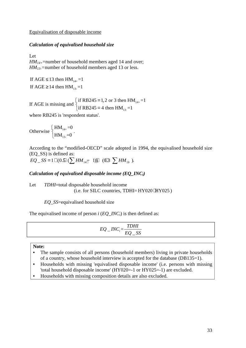
Calculation of equivalised household size Let HM14+=number of household members aged 14 and over; HM13-=number of household members aged 13 or less.

14+

13-

If AGE 13 then HM =1

If AGE 14 then HM =1

≤≥

If AGE is missing and 14+

13-

if RB245 1,2 or 3 then HM =1

if RB245 4 then HM =1

= =

where RB245 is 'respondent status'.

Otherwise 14+

13-

HM =0

HM =0

.

According to the “modified-OECD” scale adopted in 1994, the equivalised household size (EQ_SS) is defined as:

14 13_ 1 (0.5 ( 1)) (0.3 ).EQ SS HM HM+ −= + ⋅ − + ⋅∑ ∑

Calculation of equivalised disposable income (EQ_INCi) Let TDHI=total disposable household income

(i.e. for SILC countries, TDHI=HY020 HY025⋅ )

EQ_SS=equivalised household size The equivalised income of person i (EQ_INCi) is then defined as:

_ =_i

TDHIEQ INC

EQ SS

Note: • The sample consists of all persons (household members) living in private households

of a country, whose household interview is accepted for the database (DB135=1). • Households with missing 'equivalised disposable income' (i.e. persons with missing

'total household disposable income' (HY020=-1 or HY025=-1) are excluded. • Households with missing composition details are also excluded.

34

The Overarching Indicators

1. At-risk-of-poverty threshold (illustrative values)

Definition

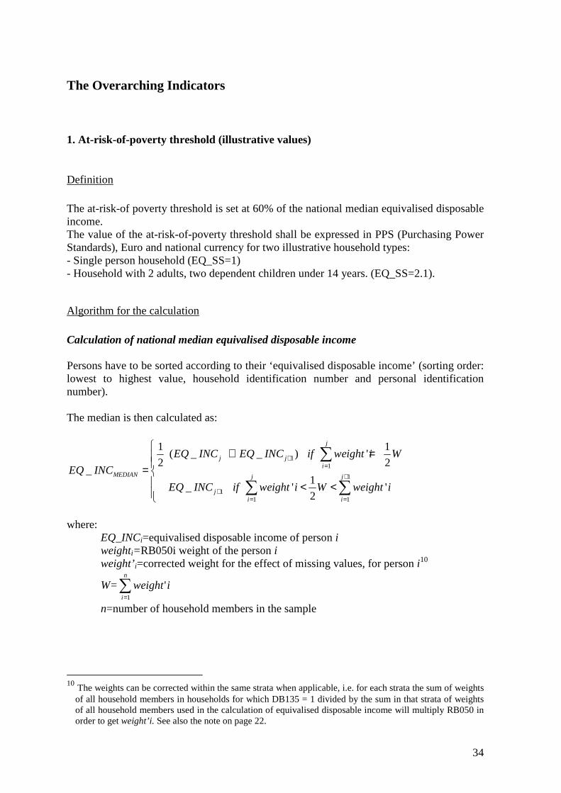
The at-risk-of poverty threshold is set at 60% of the national median equivalised disposable income. The value of the at-risk-of-poverty threshold shall be expressed in PPS (Purchasing Power Standards), Euro and national currency for two illustrative household types: - Single person household (EQ_SS=1) - Household with 2 adults, two dependent children under 14 years. (EQ_SS=2.1).

Algorithm for the calculation

Calculation of national median equivalised disposable income Persons have to be sorted according to their ‘equivalised disposable income’ (sorting order: lowest to highest value, household identification number and personal identification number). The median is then calculated as:

11

1

11 1

1 1 ( _ _ ) '

2 2_

1_ ' '

2

j

j ji

MEDIAN j j

ji i

EQ INC EQ INC if weight i W

EQ INC

EQ INC if weight i W weight i

+=

+

+= =

+ =

= < <

∑

∑ ∑

where:

EQ_INCi=equivalised disposable income of person i weighti=RB050i weight of the person i weight’i=corrected weight for the effect of missing values, for person i10

W=∑=

n

i

iweight1

'

n=number of household members in the sample

10 The weights can be corrected within the same strata when applicable, i.e. for each strata the sum of weights

of all household members in households for which DB135 = 1 divided by the sum in that strata of weights of all household members used in the calculation of equivalised disposable income will multiply RB050 in order to get weight’i. See also the note on page 22.

35

Notes: • Households (and persons therein) with missing equivalised disposable income

(EQ_INC) or any missing individual age are excluded. The median is calculated on the level of the individuals in the sample.

• Because the median is calculated at an individual level, it could happen that members of the same household (with the same equivalised disposable income) were found on different sides of the median.

Calculation of at-risk-of-poverty threshold Finally, the ‘at-risk-of-poverty threshold’ is calculated as 60% of the calculated median value, i.e.:

- - - 60% _ MEDIANARPT At risk of poverty threshold EQ INC= = ⋅

Conversion into PPS and Euro The value of the ‘at-risk-of-poverty threshold’ in national currency will be converted into EURO (for countries not in the Eurozone) and into PPS. Incomes cannot be made directly comparable by using currency exchanges rates, as the difference in purchasing power of a particular monetary unit in the different countries will not be taken into account by it. The conversion rates that take both rates of exchange and differences in purchasing power into account are called Purchasing Power Parities (PPP). They convert every national monetary unit into a common reference unit, the PPS. Note: The EUR/NAC exchange rates come from New Cronos table: Economy and finance ... Exchange rates ..…. Exchange rates …...… Bilateral exchange rates ………... Euro/ECU exchange rates …………... Euro/ECU exchange rates - Annual data ……………… UNIT: NAC ……………… OTP: Average The PPP/NAC conversion factors come from New Cronos table: Economy and finance ... Prices ..…. Purchasing power parities …...… Purchasing power parities (PPP) and comparative price level indices for the ESA95 aggregates ………… AGGREG95: EO11 Household final consumption expenditure ………… INDIC_NA: PPP_25 i.e. EU25=1 Exchange rates and PPP corresponding to the income reference period should be used. In many cases this will mean applying the conversion factors for the year preceding the survey year. For almost all countries, the rate for N-1 (survey year – 1) published on new Cronos in December of year N+1 (survey year +1) should be applied. This will be the final publication of PPP: For IE, there is an agreement to apply an arithmetic average of the rates

36

published in N+1 corresponding to the years N – 1 and N. For N the published PPS data will be preliminary. Calculation of illustrative value for the illustrative household types To illustrate the threshold values for the one person household and the two adults and two dependent children household, the ‘at-risk-of-poverty threshold’ in national currency, in Euro and in PPS will be multiplied by ‘1’ or by ‘2.1’ respectively (in line with the modified OECD-equivalence scale). Presentation table

At-risk-of-poverty threshold (illustrative values)

No Currency Rounded value

1 One-person household NAT :

2 EUR :

3 PPS :

4 2 adults, 2 dependent children under 14 years NAT :

5 EUR :

6 PPS :

2. At-risk-of-poverty rate (by age and gender)

Definition

The percentage of persons in the total population and in the relevant age and gender breakdowns, over the total population or over the relevant age or gender subset, with an equivalised disposable income below the ‘at-risk-of-poverty threshold’. The at-risk-of poverty threshold is set at 60% of the national median equivalised disposable income. For this indicator a total and breakdowns by gender and selected age groups have to be calculated.


Calculation of at-risk-of-poverty threshold See algorithm for the calculation of ‘at-risk-of-poverty threshold (illustrative values)’ (=indicator 1).

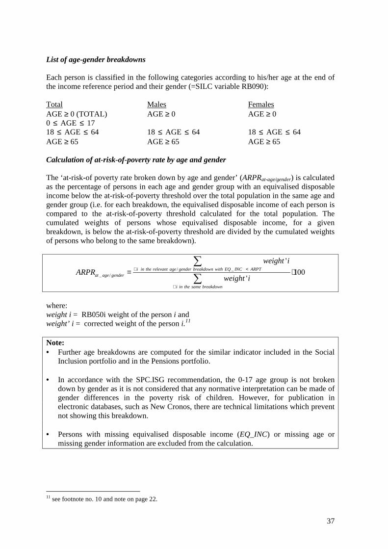
37

List of age-gender breakdowns Each person is classified in the following categories according to his/her age at the end of the income reference period and their gender (=SILC variable RB090): Total Males Females AGE ≥ 0 (TOTAL) AGE ≥ 0 AGE ≥ 0 0 ≤ AGE ≤ 17

18 ≤ AGE ≤ 64 18 ≤ AGE ≤ 64 18 ≤ AGE ≤ 64 AGE ≥ 65 AGE ≥ 65 AGE ≥ 65 Calculation of at-risk-of-poverty rate by age and gender The ‘at-risk-of poverty rate broken down by age and gender’ (ARPRat-age/gender) is calculated as the percentage of persons in each age and gender group with an equivalised disposable income below the at-risk-of-poverty threshold over the total population in the same age and gender group (i.e. for each breakdown, the equivalised disposable income of each person is compared to the at-risk-of-poverty threshold calculated for the total population. The cumulated weights of persons whose equivalised disposable income, for a given breakdown, is below the at-risk-of-poverty threshold are divided by the cumulated weights of persons who belong to the same breakdown).

/ _ _ /

'

100'

i in the relevant age gender breakdown with EQ INC ARPTat age gender

i in the same breakdown

weight i

ARPRweight i

∀ <

∀

= ⋅∑

∑

where: weight i = RB050i weight of the person i and weight’ i = corrected weight of the person i.11 Note: • Further age breakdowns are computed for the similar indicator included in the Social

Inclusion portfolio and in the Pensions portfolio. • In accordance with the SPC.ISG recommendation, the 0-17 age group is not broken

down by gender as it is not considered that any normative interpretation can be made of gender differences in the poverty risk of children. However, for publication in electronic databases, such as New Cronos, there are technical limitations which prevent not showing this breakdown.

• Persons with missing equivalised disposable income (EQ_INC) or missing age or

missing gender information are excluded from the calculation.

11 see footnote no. 10 and note on page 22.

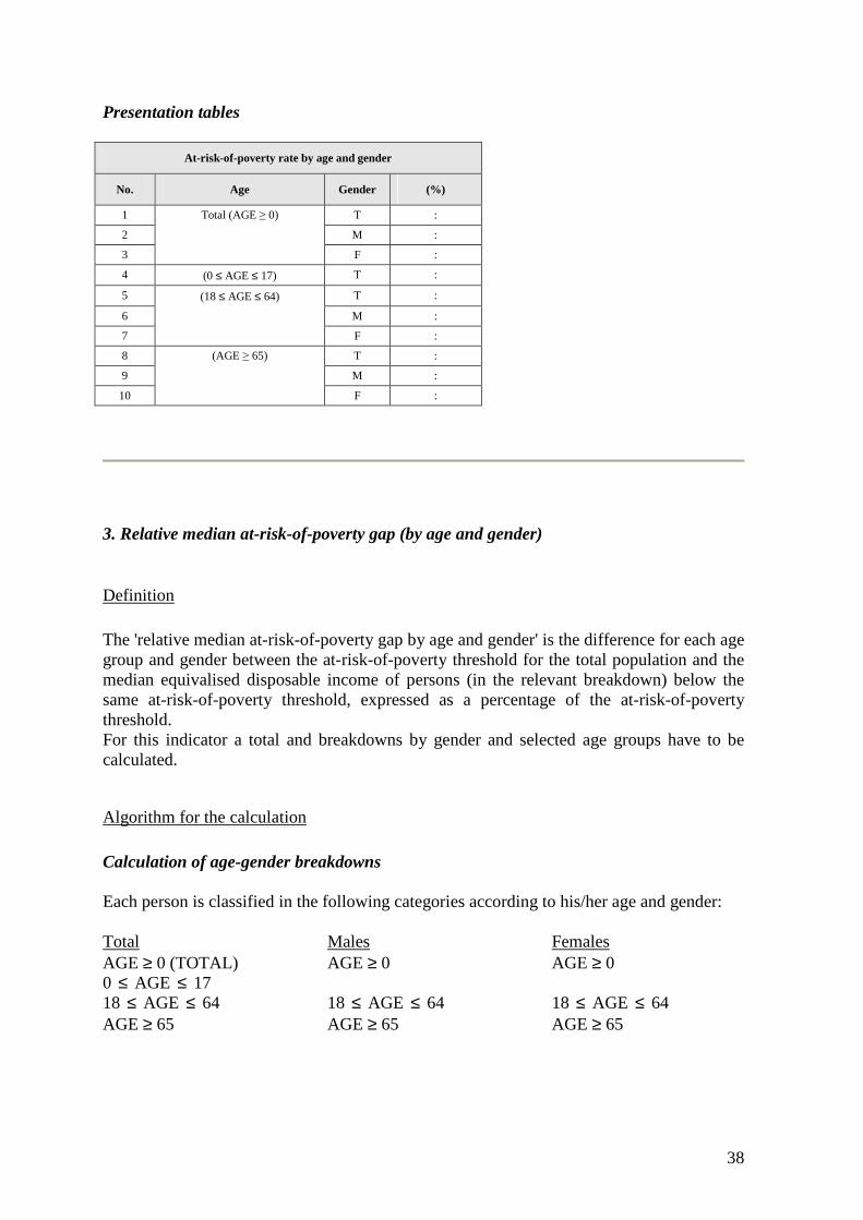
38

Presentation tables

At-risk-of-poverty rate by age and gender

No. Age Gender (%)

1 Total (AGE ≥ 0) T :

2 M :

3 F :

4 (0 ≤ AGE ≤ 17) T :

5 (18 ≤ AGE ≤ 64) T :

6 M :

7 F :

8 (AGE ≥ 65) T :

9 M :

10 F :

3. Relative median at-risk-of-poverty gap (by age and gender)

Definition

The 'relative median at-risk-of-poverty gap by age and gender' is the difference for each age group and gender between the at-risk-of-poverty threshold for the total population and the median equivalised disposable income of persons (in the relevant breakdown) below the same at-risk-of-poverty threshold, expressed as a percentage of the at-risk-of-poverty threshold. For this indicator a total and breakdowns by gender and selected age groups have to be calculated.


Calculation of age-gender breakdowns Each person is classified in the following categories according to his/her age and gender: Total Males Females AGE ≥ 0 (TOTAL) AGE ≥ 0 AGE ≥ 0 0 ≤ AGE ≤ 17 18 ≤ AGE ≤ 64 18 ≤ AGE ≤ 64 18 ≤ AGE ≤ 64 AGE ≥ 65 AGE ≥ 65 AGE ≥ 65

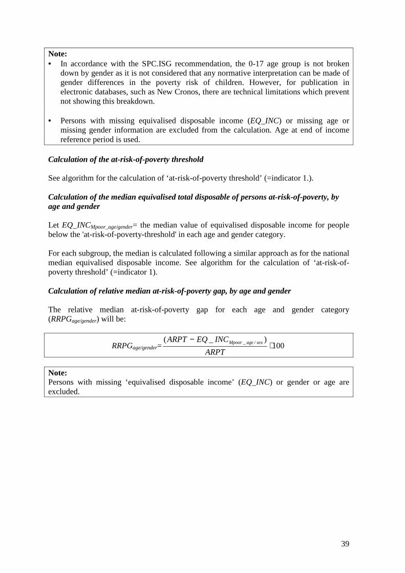
39

Note: • In accordance with the SPC.ISG recommendation, the 0-17 age group is not broken


• Persons with missing equivalised disposable income (EQ_INC) or missing age or

missing gender information are excluded from the calculation. Age at end of income reference period is used.

Calculation of the at-risk-of-poverty threshold See algorithm for the calculation of ‘at-risk-of-poverty threshold’ (=indicator 1.). Calculation of the median equivalised total disposable of persons at-risk-of-poverty, by age and gender Let EQ_INCMpoor_age/gender= the median value of equivalised disposable income for people below the 'at-risk-of-poverty-threshold' in each age and gender category.

For each subgroup, the median is calculated following a similar approach as for the national median equivalised disposable income. See algorithm for the calculation of ‘at-risk-of-poverty threshold’ (=indicator 1). Calculation of relative median at-risk-of-poverty gap, by age and gender The relative median at-risk-of-poverty gap for each age and gender category (RRPGage/gender) will be:

RRPGage/gender= 100)_( /_ ⋅

−ARPT

INCEQARPT sexageMpoor

Note: Persons with missing ‘equivalised disposable income’ (EQ_INC) or gender or age are excluded.

40

Presentation table

Relative median at-risk-of poverty gap

No. Age Gender (%)


2 M :

3 F :

4 (0 ≤ AGE ≤ 17) T :

5 (18 ≤ AGE ≤ 64) T :

6 M :

7 F :

8 (AGE ≥ 65) T :

9 M :

10 F :

4. At-risk-of-poverty rate anchored at a fixed moment in time (2005) (by age and gender)

Comment

A similar indicator was previously calculated from the ECHP survey, but suspended during the transition to SILC. Because of concerns about the complexity of the indicator previously calculated the definition and focus of this indicator has been slightly changed in the ISG. Instead of a moving anchor, the reference threshold is now a fixed anchor. As before, the focus is on whether general improvements in living standards are successful in lifting people out of poverty (or at least increasing their real income). The current definition is tentative and not yet agreed at the level of the ISG. Some refining can be envisaged. The base or reference year (currently 2005) is meant to change in regular intervals. Specific attention needs to be paid to the adjustment for inflation. Note: The definition of this indicator is a tentative proposal liable to change as it does not correspond in all details to the definition agreed at the SPC in June 2006. This definition will be proposed to the ISG.

Definition

For a given year ‘T’, the ‘at-risk-of-poverty rate anchored at a fixed moment in time (2005)’ is defined as the percentage of the population whose equivalised total disposable income in that given year is below the ‘at-risk-of-poverty threshold’ calculated in the standard way for the reference year or base year, currently 2005, and then adjusted for inflation.

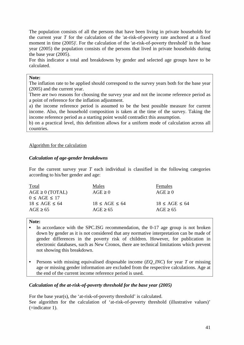
41

The population consists of all the persons that have been living in private households for the current year T for the calculation of the 'at-risk-of-poverty rate anchored at a fixed moment in time (2005)'. For the calculation of the 'at-risk-of-poverty threshold' in the base year (2005) the population consists of the persons that lived in private households during the base year (2005). For this indicator a total and breakdowns by gender and selected age groups have to be calculated. Note: The inflation rate to be applied should correspond to the survey years both for the base year (2005) and the current year. There are two reasons for choosing the survey year and not the income reference period as a point of reference for the inflation adjustment. a) the income reference period is assumed to be the best possible measure for current income. Also, the household composition is taken at the time of the survey. Taking the income reference period as a starting point would contradict this assumption. b) on a practical level, this definition allows for a uniform mode of calculation across all countries.


Calculation of age-gender breakdowns For the current survey year T each individual is classified in the following categories according to his/her gender and age: Total Males Females AGE ≥ 0 (TOTAL) AGE ≥ 0 AGE ≥ 0 0 ≤ AGE ≤ 17 18 ≤ AGE ≤ 64 18 ≤ AGE ≤ 64 18 ≤ AGE ≤ 64 AGE ≥ 65 AGE ≥ 65 AGE ≥ 65 Note: • In accordance with the SPC.ISG recommendation, the 0-17 age group is not broken


• Persons with missing equivalised disposable income (EQ_INC) for year T or missing

age or missing gender information are excluded from the respective calculations. Age at the end of the current income reference period is used.

Calculation of the at-risk-of-poverty threshold for the base year (2005) For the base year(s), the ‘at-risk-of-poverty threshold’ is calculated. See algorithm for the calculation of ‘at-risk-of-poverty threshold (illustrative values)’ (=indicator 1).

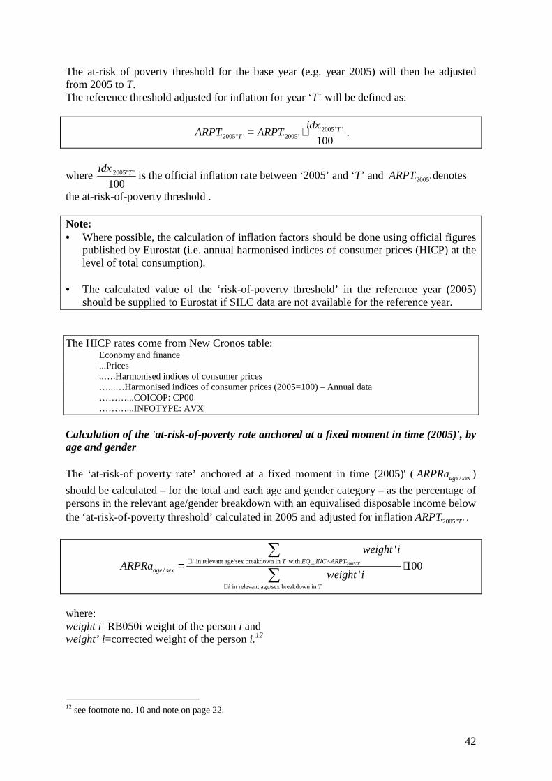
42

The at-risk of poverty threshold for the base year (e.g. year 2005) will then be adjusted from 2005 to T. The reference threshold adjusted for inflation for year ‘T’ will be defined as:

'2005'' ''2005'' ' '2005' 100

TT

idxARPT ARPT= ⋅ ,

where '2005'' '

100Tidx

is the official inflation rate between ‘2005’ and ‘T’ and '2005'ARPT denotes

the at-risk-of-poverty threshold . Note: • Where possible, the calculation of inflation factors should be done using official figures

published by Eurostat (i.e. annual harmonised indices of consumer prices (HICP) at the level of total consumption).

• The calculated value of the ‘risk-of-poverty threshold’ in the reference year (2005)

should be supplied to Eurostat if SILC data are not available for the reference year. The HICP rates come from New Cronos table: Economy and finance ...Prices ..….Harmonised indices of consumer prices …...…Harmonised indices of consumer prices (2005=100) – Annual data ………...COICOP: CP00 ………...INFOTYPE: AVX

Calculation of the 'at-risk-of-poverty rate anchored at a fixed moment in time (2005)', by age and gender The ‘at-risk-of poverty rate’ anchored at a fixed moment in time (2005)' ( /age sexARPRa )

should be calculated – for the total and each age and gender category – as the percentage of persons in the relevant age/gender breakdown with an equivalised disposable income below the ‘at-risk-of-poverty threshold’ calculated in 2005 and adjusted for inflation '2005'' 'TARPT .

'2005'' ' in relevant age/sex breakdown in with _ </

in relevant age/sex breakdown in

'

100'

Ti T EQ INC ARPTage sex

i T

weight i

ARPRaweight i

∀

∀

= ⋅∑

∑

where: weight i=RB050i weight of the person i and weight’ i=corrected weight of the person i.12


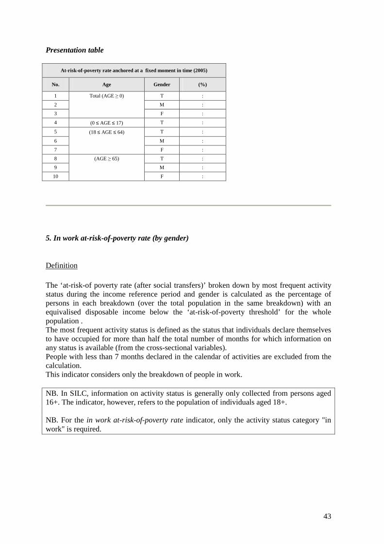
43

Presentation table

At-risk-of-poverty rate anchored at a fixed moment in time (2005)

No. Age Gender (%)


2 M :

3 F :

4 (0 ≤ AGE ≤ 17) T :

5 (18 ≤ AGE ≤ 64) T :

6 M :

7 F :

8 (AGE ≥ 65) T :

9 M :

10 F :

5. In work at-risk-of-poverty rate (by gender)

Definition

The ‘at-risk-of poverty rate (after social transfers)’ broken down by most frequent activity status during the income reference period and gender is calculated as the percentage of persons in each breakdown (over the total population in the same breakdown) with an equivalised disposable income below the ‘at-risk-of-poverty threshold’ for the whole population . The most frequent activity status is defined as the status that individuals declare themselves to have occupied for more than half the total number of months for which information on any status is available (from the cross-sectional variables). People with less than 7 months declared in the calendar of activities are excluded from the calculation. This indicator considers only the breakdown of people in work. NB. In SILC, information on activity status is generally only collected from persons aged 16+. The indicator, however, refers to the population of individuals aged 18+. NB. For the in work at-risk-of-poverty rate indicator, only the activity status category "in work" is required.

44


Calculation of age-gender breakdowns Each household member is classified according to their gender. Note: A breakdown by age is considered only for the corresponding Social Inclusion indicator. Activity status information is only considered relevant for persons aged 18+. Calculation of most frequent activity status breakdowns For each household member for which RB250 = 11, 12 or 13 the following variables will be selected: PL070, PL072, PL080, PL085, PL087, PL090. The following derived variables will be constructed: TOT= PL070 + PL072 + PL080 + PL085 + PL087 + PL090 WRK= PL070 + PL072 If TOT < 7 , then exclude the individual.

(Only persons, which have reported for more than 7 months are considered.)

If TOT 7≥ 1WRK

RatioTOT

=

(The calculations above determine, what ratio of time was spent in 'in work' for each person.) If 1Ratio ≤ 0.5 , then exclude the individual. (Here it is determined whether the person has spent more than half the reported time in 'in work') Otherwise: - if Ratio1 > 0.5 1=⇒ statusActivity (The person is considered to be 'in work'). Note: • Only the persons with activity status 1 ('in work') are to be considered for this indicator. • The activity statuses correspond to the following SILC target variables:

cross-sectional survey: WRK = sum of PL070 (full-time) and PL072 (part-time)

Calculation of in work at-risk-of-poverty rate by gender The 'in work-at-risk-of poverty rate (after social transfers)' broken down by gender (ARPR

iw-gender) is calculated as the percentage of persons 'in work' with an equivalised disposable income below the ‘at-risk-of-poverty threshold’ over the total population in that breakdown (i.e. for each gender, the equivalised disposable income of each person 'in work' is compared with the at-risk-of-poverty threshold calculated for the total population. The

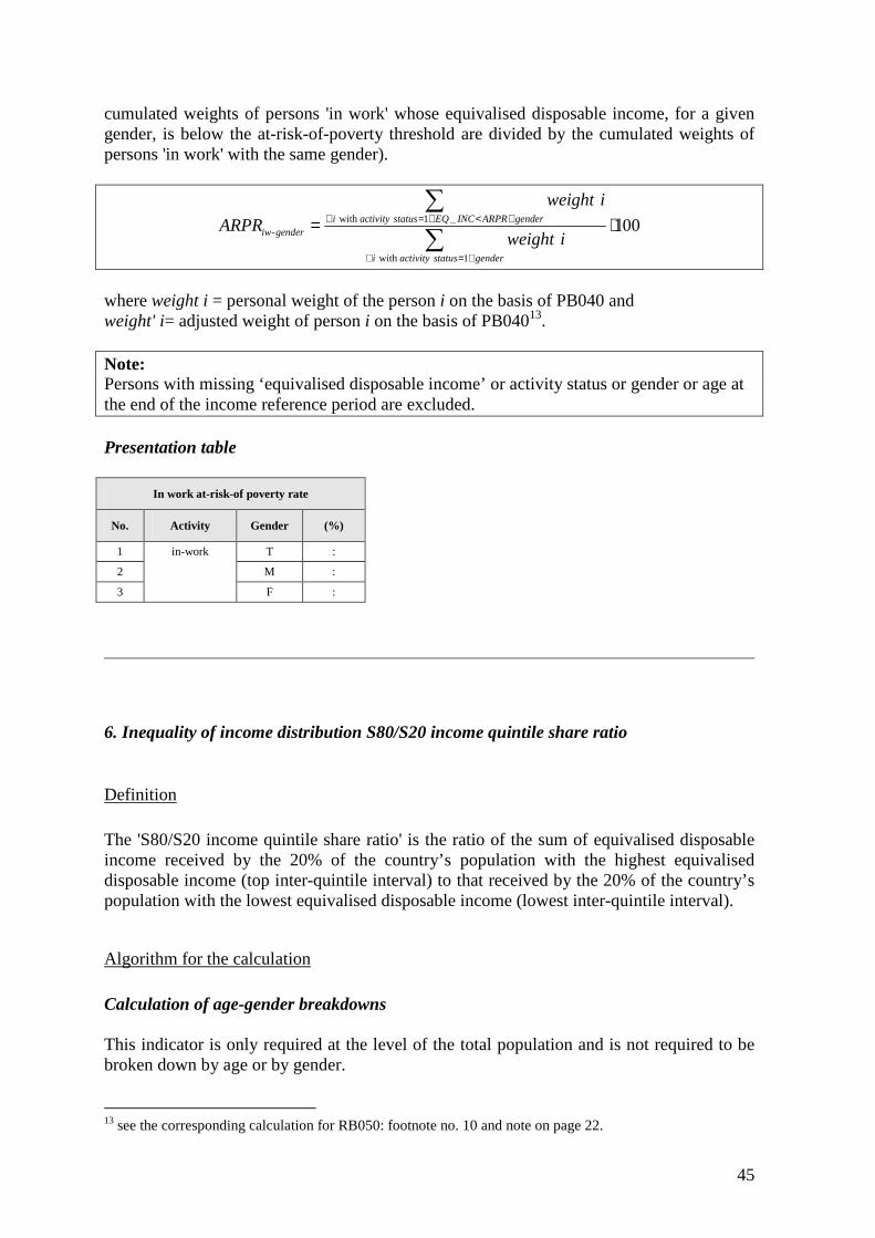
45

cumulated weights of persons 'in work' whose equivalised disposable income, for a given gender, is below the at-risk-of-poverty threshold are divided by the cumulated weights of persons 'in work' with the same gender).

with 1 _-

with 1

100

i activity status EQ INC ARPR genderiw gender

i activity status gender

weight i

ARPRweight i

∀ = ∧ < ∧

∀ = ∧

= ⋅∑

∑

where weight i = personal weight of the person i on the basis of PB040 and weight' i= adjusted weight of person i on the basis of PB04013. Note: Persons with missing ‘equivalised disposable income’ or activity status or gender or age at the end of the income reference period are excluded. Presentation table

In work at-risk-of poverty rate

No. Activity Gender (%)

1 in-work T :

2 M :

3 F :

6. Inequality of income distribution S80/S20 income quintile share ratio

Definition

The 'S80/S20 income quintile share ratio' is the ratio of the sum of equivalised disposable income received by the 20% of the country’s population with the highest equivalised disposable income (top inter-quintile interval) to that received by the 20% of the country’s population with the lowest equivalised disposable income (lowest inter-quintile interval).


Calculation of age-gender breakdowns This indicator is only required at the level of the total population and is not required to be broken down by age or by gender. 13 see the corresponding calculation for RB050: footnote no. 10 and note on page 22.

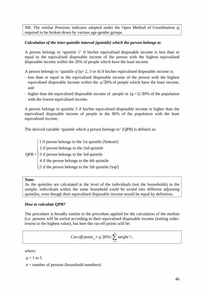
46

NB. The similar Pensions indicator adopted under the Open Method of Coordination is required to be broken down by various age-gender groups. Calculation of the inter-quintile interval (quintile) which the person belongs to A person belongs to ‘quintile 1’ if his/her equivalised disposable income is less than or equal to the equivalised disposable income of the person with the highest equivalised disposable income within the 20% of people which have the least income. A person belongs to ‘quintile q’(q= 2, 3 or 4) if his/her equivalised disposable income is:

- less than or equal to the equivalised disposable income of the person with the highest equivalised disposable income within the 20%q ⋅ of people which have the least income, and

- higher than the equivalised disposable income of people in ( 1) 20%q − ⋅ of the population with the lowest equivalised income.

A person belongs to quintile 5 if his/her equivalised disposable income is higher than the equivalised disposable income of people in the 80% of the population with the least equivalised income.

The derived variable ‘quintile which a person belongs to’ (QPB) is defined as:

1 if person belongs to the 1st quintile ('bottom')

2 if person belongs to the 2nd quintile

QPB = 3 if person belongs to the 3rd quintile

4 if the person belongs to the 4th quintile

5 if the person belongs to the 5th quintile ('top')

Note: As the quintiles are calculated at the level of the individuals (not the households) in the sample, individuals within the same household could be sorted into different adjoining quintiles, even though their equivalised disposable income would be equal by definition. How to calculate QPB? The procedure is broadly similar to the procedure applied for the calculation of the median (i.e. persons will be sorted according to their equivalised disposable income (sorting order: lowest to the highest value), but here the cut-off points will be:

Cut-off-point1

20% 'n

qi

q weight i=

= ⋅ ⋅∑ ,

where:

q = 1 to 5

n = number of persons (household members)

47

weight’i = is the corrected weight of person i.

W=∑=

n

i

iweight1

'

( )11

_ 1

11 1

1_ _ ' 20%

2_

_ ' 20% '

j

j ji

q quintile j j

ji i

EQ INC EQ INC if weight i q W

EQ INC

EQ INC if weight i q W weight i

+=

+

+= =

+ = ⋅ ⋅

< ⋅ ⋅ <

∑

∑ ∑

Note: Persons with missing ‘equivalised disposable income’ are excluded. Calculation of the S80/S20 income quintile share ratio The S80/S20 income quintile share ratio should be the ratio of the sum of equivalised disposable income received by the 20% of the country’s population with the highest equivalised disposable income (top inter-quintile interval) to that received by the 20% of the country’s population with the lowest equivalised disposable income (lowest inter-quintile interval), i.e.

5

1

' _

80 / 20' _

ii QPB

ii QPB

weight i EQ INC

S Sweight i EQ INC

∈ =

∈ =

⋅=

⋅

∑

∑

weight’i = is the corrected weight of person i based on RB050.14 Presentation table

S80/S20 income quintile share ratio

Ratio

Total population :

7. Relative median income ratio

Comment

The relative median income ratio is a measure of the degree to which the incomes of persons in the upper age group (aged 65 or over) are higher than or lower than the incomes of persons in the lower age group (aged under 65). 14 see footnote no. 10 and note on page 22.

48

Definition

The ratio of the median equivalised disposable income of persons aged above the specified age limit (aged 65 or over) to the median equivalised disposable income of persons in complementary age groups (aged between 0 and 64).


First median equivalised disposable incomes for those age 65+ and those aged between 0-64 have to be calculated. For this corrected weights based on RB050 have to be used.15

(65 )

(0 64)

_

_MEDIAN

MEDIAN

EQ INCRMIRa

EQ INC+

−

=

Note: Households which contain individuals with missing ‘equivalised disposable income’ (EQ_INC) or gender or age are excluded. Age at the end of the income reference period is used. Presentation table

Relative median income ratio

No. Age groups Gender (%)

1 65+ / 0-64 T :

8. Aggregate replacement ratio Background This indicator was intensively discussed in the Indicator Sub Group of the Social Protection Committee. Finally it was agreed that an indicator should be developed to focus on "the transition in income status of the individual" arising from working to retirement. Consequently, it refers to specific individual income components that, by definition, are recorded as gross components in EU-SILC16. Equivalisation is thus not performed in this case, because it is inappropriate.

15 see footnote no. 10 and note on page 22. 16 Those countries currently unable to supply the relevant gross income components should provide results based on the corresponding net income components. From the 2007 data collection onwards, this indicator should be calculated on the basis of gross income in all countries.

49

Note: Up to and including the year 2006, gross income components were used for the calculation of this indicator where gross components were available. Net components were use where only net components were available. From the year 2007 onwards, only gross components are used. Thus for those countries which were unable to provide gross components up to 2007, this represents a significant change in methodology (and values of the indicator). This change will be indicated as a break in series. Due to these methodological choices, special attention is required in interpretation of the aggregate replacement ratio. The aggregate replacement ratio is a crude measure of comparison of the pension income of individuals in the upper age group and the income from work of persons in the lower age group. Deliberately, no account is taken of other income sources like investment income or social transfers between households. It should be taken into account that this aggregate calculation does not in fact compare the situation of the same individuals before and after the cut-off age. Moreover, as this calculation is done using non-equivalised income, no account is taken of differences in household composition or size, which may affect the adequacy of the income.

Definition

This indicator is the ratio of the median personal (non-equivalised) income from pensions of retired persons aged 65-74, to the median personal (non-equivalised) income from earnings of persons in work aged 50-59. For this indicator, breakdowns by gender have to be provided in addition to the total.


Calculation of activity statuses retired and in work for the 'aggregate replacement ratio' Note: • In the context of the calculation of this indicator, the calculation of the 'activity status differs from that used in other indicators. • The aggregate replacement ratio is based exclusively on the variables available in the cross-sectional sample A person is considered to be 'in work' if PL070+PL072=12. A person is considered to be 'retired' if PL085=12. That is, a person 'retired' or 'in work' if and only if he/ she has been 'retired' or 'in work' for all the months in the income reference period. This type of calculation is likely to exclude a significant amount of persons who were mainly retired or in work from the calculations (and might introduce an age bias) but avoids problems of a bias of income from the respective activity. Calculation of relevant income Different definitions of income are used for each of the separate age/activity status:

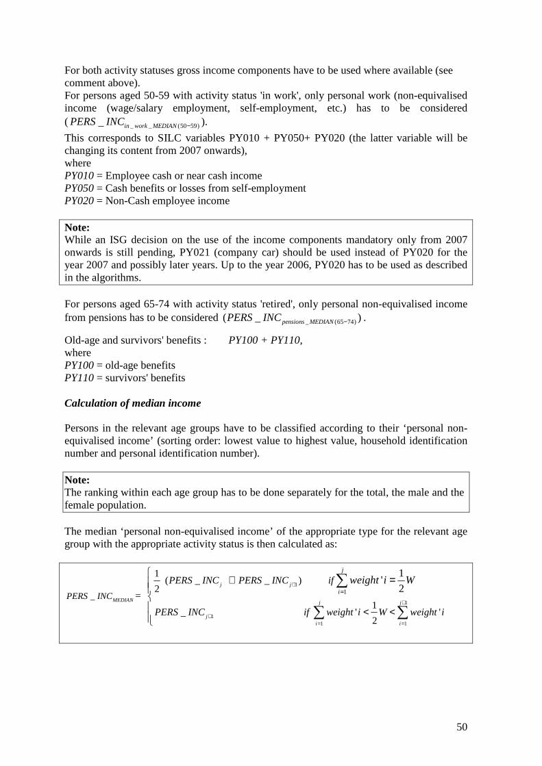
50

For both activity statuses gross income components have to be used where available (see comment above). For persons aged 50-59 with activity status 'in work', only personal work (non-equivalised income (wage/salary employment, self-employment, etc.) has to be considered ( _ _ (50 59)_ in work MEDIANPERS INC − ).

This corresponds to SILC variables PY010 + PY050+ PY020 (the latter variable will be changing its content from 2007 onwards), where PY010 = Employee cash or near cash income PY050 = Cash benefits or losses from self-employment PY020 = Non-Cash employee income Note: While an ISG decision on the use of the income components mandatory only from 2007 onwards is still pending, PY021 (company car) should be used instead of PY020 for the year 2007 and possibly later years. Up to the year 2006, PY020 has to be used as described in the algorithms. For persons aged 65-74 with activity status 'retired', only personal non-equivalised income from pensions has to be considered _ (65 74)( _ )pensions MEDIANPERS INC − .

Old-age and survivors' benefits : PY100 + PY110, where PY100 = old-age benefits PY110 = survivors' benefits Calculation of median income Persons in the relevant age groups have to be classified according to their ‘personal non- equivalised income’ (sorting order: lowest value to highest value, household identification number and personal identification number). Note: The ranking within each age group has to be done separately for the total, the male and the female population. The median ‘personal non-equivalised income’ of the appropriate type for the relevant age group with the appropriate activity status is then calculated as:

1

1

11 1

1_

1 ( _ _ )

2=

1_ ' '

2

1'

2j j

MEDIAN j j

ji i

j

iPERS INC

PERS INC PERS INC if

PERS INC if weight i W weight i

weight i W+

+

+= =

=

+

< <

=

∑ ∑

∑

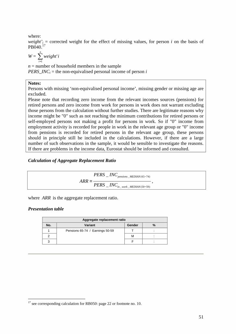
51

where: weight’i = corrected weight for the effect of missing values, for person i on the basis of PB040.17

W = ∑=

n

i

iweight1

'

n = number of household members in the sample PERS_INCi = the non-equivalised personal income of person i Notes: Persons with missing ‘non-equivalised personal income’, missing gender or missing age are excluded. Please note that recording zero income from the relevant incomes sources (pensions) for retired persons and zero income from work for persons in work does not warrant excluding those persons from the calculation without further studies. There are legitimate reasons why income might be "0" such as not reaching the minimum contributions for retired persons or self-employed persons not making a profit for persons in work. So if "0" income from employment activity is recorded for people in work in the relevant age group or "0" income from pensions is recorded for retired persons in the relevant age group, these persons should in principle still be included in the calculations. However, if there are a large number of such observations in the sample, it would be sensible to investigate the reasons. If there are problems in the income data, Eurostat should be informed and consulted. Calculation of Aggregate Replacement Ratio

_ (65 74)

_ _ (50 59)

_

_

pensions MEDIAN

in work MEDIAN

PERS INCARR

PERS INC

−

−

= ,

where ARR is the aggregate replacement ratio. Presentation table

Aggregate replacement ratio

No. Variant Gender %

1 Pensions 65-74 / Earnings 50-59 T :

2 M :

3 F :

17 see corresponding calculation for RB050: page 22 or footnote no. 10.

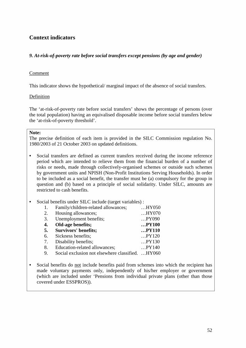
52

Context indicators

9. At-risk-of-poverty rate before social transfers except pensions (by age and gender)

Comment

This indicator shows the hypothetical/ marginal impact of the absence of social transfers.

Definition

The ‘at-risk-of-poverty rate before social transfers’ shows the percentage of persons (over the total population) having an equivalised disposable income before social transfers below the ‘at-risk-of-poverty threshold’. Note: The precise definition of each item is provided in the SILC Commission regulation No. 1980/2003 of 21 October 2003 on updated definitions. • Social transfers are defined as current transfers received during the income reference

period which are intended to relieve them from the financial burden of a number of risks or needs, made through collectively-organised schemes or outside such schemes by government units and NPISH (Non-Profit Institutions Serving Households). In order to be included as a social benefit, the transfer must be (a) compulsory for the group in question and (b) based on a principle of social solidarity. Under SILC, amounts are restricted to cash benefits.

• Social benefits under SILC include (target variables) : 1. Family/children-related allowances; …HY050 2. Housing allowances; …HY070 3. Unemployment benefits; …PY090 4. Old-age benefits; …PY100 5. Survivors' benefits; …PY110 6. Sickness benefits; …PY120 7. Disability benefits; …PY130 8. Education-related allowances; …PY140 9. Social exclusion not elsewhere classified. …HY060 • Social benefits do not include benefits paid from schemes into which the recipient has

made voluntary payments only, independently of his/her employer or government (which are included under ‘Pensions from individual private plans (other than those covered under ESSPROS)).

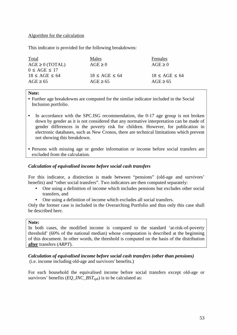
53


This indicator is provided for the following breakdowns: Total Males Females AGE ≥ 0 (TOTAL) AGE ≥ 0 AGE ≥ 0 0 ≤ AGE ≤ 17 18 ≤ AGE ≤ 64 18 ≤ AGE ≤ 64 18 ≤ AGE ≤ 64 AGE ≥ 65 AGE ≥ 65 AGE ≥ 65 Note: • Further age breakdowns are computed for the similar indicator included in the Social

Inclusion portfolio. • In accordance with the SPC.ISG recommendation, the 0-17 age group is not broken

down by gender as it is not considered that any normative interpretation can be made of gender differences in the poverty risk for children. However, for publication in electronic databases, such as New Cronos, there are technical limitations which prevent not showing this breakdown.

• Persons with missing age or gender information or income before social transfers are

excluded from the calculation. Calculation of equivalised income before social cash transfers For this indicator, a distinction is made between “pensions” (old-age and survivors’ benefits) and “other social transfers”. Two indicators are then computed separately:

• One using a definition of income which includes pensions but excludes other social transfers, and

• One using a definition of income which excludes all social transfers. Only the former case is included in the Overarching Portfolio and thus only this case shall be described here. Note: In both cases, the modified income is compared to the standard ‘at-risk-of-poverty threshold’ (60% of the national median) whose computation is described at the beginning of this document. In other words, the threshold is computed on the basis of the distribution after transfers (ARPT). Calculation of equivalised income before social cash transfers (other than pensions) (i.e. income including old-age and survivors' benefits.) For each household the equivalised income before social transfers except old-age or survivors’ benefits (EQ_INC_BSTepb) is to be calculated as:

54

HY022 HY025_ _

_epbEQ INC BSTEQ SS

⋅= ,18

( )_ HY022 HY025

HY020- HY050+HY070+HY090+PY120+PY130+PY140+HY060 HY025

epbINC BST = ⋅ =

= ⋅

Each person in the same household receives the same total equivalised disposable income before social transfers except old-age and survivors benefits (EQ_INC_BSTepb). Calculation of 'at-risk-of-poverty rate before social transfers except old-age and survivors’ benefits', by age and gender The ‘at-risk-of-poverty rate before social transfers except old-age and survivors’ benefits broken down by age and gender’ (ARPR_BSTepb-at-age/gender) is calculated – for each gender and age category – as the percentage of persons (over the total population) with an equivalised disposable income before social transfers except old-age and survivors’ benefits (EQ_INC_BSTepb-at-age/gender) below the ‘at-risk-of-poverty threshold’ (i.e. for each breakdown, the equivalised disposable income before social transfers except old-age and survivors’ benefits of each person is compared with the at-risk-of-poverty threshold. The cumulated weights of people whose equivalised disposable income, for a given breakdown, is below the at-risk-of-poverty threshold are divided by the cumulated weights of persons who belong to the same breakdown).

/ _ _

/

/

'

_ 100'

epbi in each age gender breakdown with EQ INC BST ARPT

epb at age gender

i in the same age gender breakdown

weight i

ARPR BSTweight i

∀ <− −

∀

= ⋅∑

∑,

where weight’i = is the corrected weight of person i. Note: • The ‘at-risk-of-poverty threshold’ (60% of the national median) is the same as the one

used to calculate the at-risk-of-poverty rate after transfers. In other words, the threshold is computed on the basis of the distribution of income after transfers (ARPT).

• Persons with missing ‘equivalised disposable income before transfers except old-age and survivors benefits’ (EQ_INC_BSTepb) and/or missing age and/or missing gender are excluded.

18 The estimation of equivalised disposable income before transfer in case of missing individuals is based on the assumption that the impact of missing values is the same on HY020, HY022 and HY023 (constant factor).

55

Presentation table

At-risk-of-poverty rate before social transfers except old-age and survivors’ benefits

No. Age Gender (%)


2 M :

3 F :

4 (0 ≤ AGE ≤ 17) T :

5 (18 ≤ AGE ≤ 64) T :

6 M :

7 F :

8 (AGE ≥ 65) T :

9 M :

10 F :

10. Distribution of population by household types

Definition

The distribution of the population by household type is calculated as the percentage of persons in each category of over the total population. The analysis is required for:

(a) the total population, and (b) the ‘poor’ population.

A person is considered to be ‘poor’ if his/her equivalised disposable income is below the ‘at-risk-of- poverty threshold after social transfers’: i.e. if the person if considered to be living in a household at risk of poverty. This distribution information is intended to complement the calculation of the corresponding incidence measure (‘at-risk-of-poverty rate’).


Calculation of household type breakdowns Each person is classified into the following household type breakdowns as for the corresponding incidence indicator. The following household types will be considered:

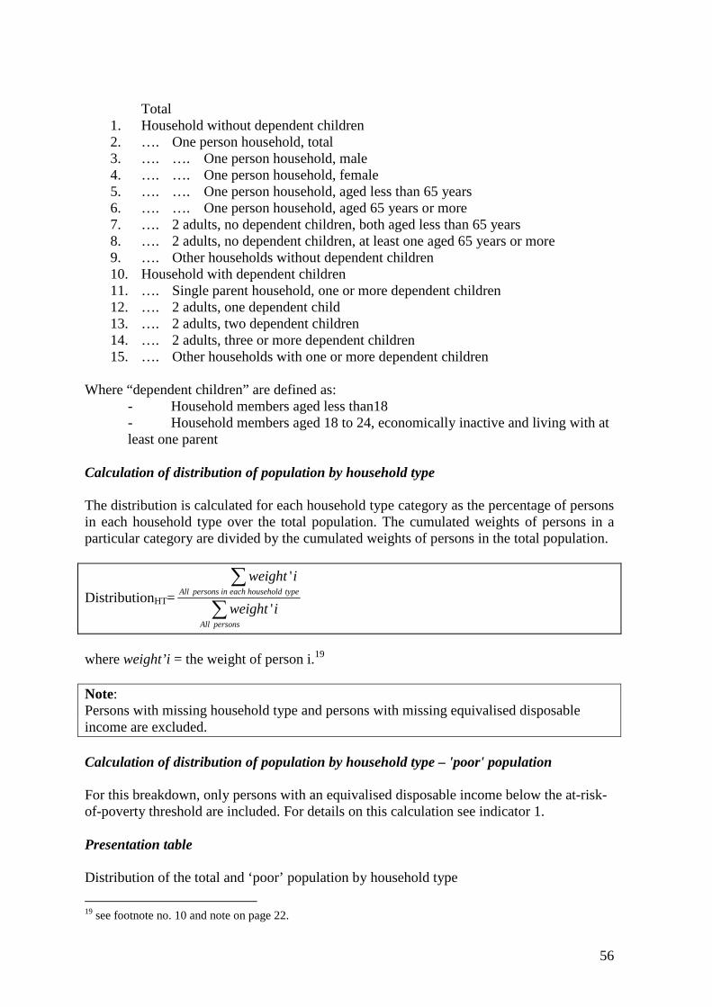
56

Total 1. Household without dependent children 2. …. One person household, total 3. …. …. One person household, male 4. …. …. One person household, female 5. …. …. One person household, aged less than 65 years 6. …. …. One person household, aged 65 years or more 7. …. 2 adults, no dependent children, both aged less than 65 years 8. …. 2 adults, no dependent children, at least one aged 65 years or more 9. …. Other households without dependent children 10. Household with dependent children 11. …. Single parent household, one or more dependent children 12. …. 2 adults, one dependent child 13. …. 2 adults, two dependent children 14. …. 2 adults, three or more dependent children 15. …. Other households with one or more dependent children Where “dependent children” are defined as:

- Household members aged less than18 - Household members aged 18 to 24, economically inactive and living with at least one parent

Calculation of distribution of population by household type The distribution is calculated for each household type category as the percentage of persons in each household type over the total population. The cumulated weights of persons in a particular category are divided by the cumulated weights of persons in the total population.

DistributionHT=∑

∑

personsAll

typehouseholdeachinpersonsAll

iweight

iweight

'

'

where weight’i = the weight of person i.19 Note: Persons with missing household type and persons with missing equivalised disposable income are excluded. Calculation of distribution of population by household type – 'poor' population For this breakdown, only persons with an equivalised disposable income below the at-risk-of-poverty threshold are included. For details on this calculation see indicator 1. Presentation table Distribution of the total and ‘poor’ population by household type


57

Distribution of population by household types

Household without dependent children Household with dependent children Total

1 2 3 4 5 6 7 8 9 10 11 12 13 14 15

Total 100

Poor 100

58

APPENDIX I: The EU-SILC Legal Framework (situation as at January 2009)

Details of the methodology applicable for participant countries with effect from 2003 (launch under gentlemen’s agreement) and 2004 (under regulation). Framework Regulations:

Regulation of the European Parliament and of the Council (EC) No.1177/2003, dated 16 June 2003, concerning Community statistics on income and living conditions (EU-SILC): text with EEA relevance, published in Official Journal L 165, 3/7/2003 P.0001-0009.

Regulation of the European Parliament and of the Council (EC) No.1553/2005, dated 7 September 2005, amending Regulation (EC) No.1177/2003 concerning Community statistics on income and living conditions (EU-SILC): text with EEA relevance, published in Official Journal L 255, 30/9/2005 P.0006-0008.

Implementation Regulations:

Commission Regulation (EC) No.1980/2003, dated 21st October 2003, implementing Regulation (EC) No.1177/2003…(EU-SILC) as regards definitions and updated definitions: text with EEA relevance, published in Official Journal L.298, 17/11/2003 P.0001-0022.

Commission Regulation (EC) No.1981/2003, dated 21st October 2003, implementing Regulation (EC) No.1177/2003…(EU-SILC) as regards fieldwork aspects and imputation procedures: text with EEA relevance, published in Official Journal L.298, 17/11/2003 P.0023-0028.

Commission Regulation (EC) No.1982/2003, dated 21st October 2003, implementing Regulation (EC) No.1177/2003…(EU-SILC) as regards sampling and tracing rules: text with EEA relevance, published in Official Journal L.298, 17/11/2003 P.0029-0033.

Commission Regulation (EC) No.1983/2003, dated 7th November 2003, implementing Regulation (EC) No.1177/2003…(EU-SILC) as regards the list of primary target variables: text with EEA relevance, published in Official Journal L.298, 17/11/2003 P.0034-0085.

Commission Regulation (EC) No.28/2004, dated 5th January 2004, implementing Regulation (EC) No.1177/2003…(EU-SILC) as regards the detailed content of intermediate and final quality reports: text with EEA relevance, published in Official Journal L.5, 9/1/2004 P.0042-0056.

Current Regulations on Modules:

2005 - Commission Regulation (EC) No.16/2004, dated 6th January 2004, implementing Regulation (EC) No.1177/2003…(EU-SILC) as regards the target list of secondary variables relating to “the intergenerational transmission of poverty” : text with EEA relevance, published in Official Journal L.4, 8/1/2004 P.0003-0006.

2006 - Commission Regulation (EC) No.13/2005, dated 6th January 2005, implementing Regulation (EC) No.1177/2003…(EU-SILC) as regards the target list of secondary variables relating to “social participation” : text with EEA relevance, published in Official Journal L.5, 7/1/2005 P.0005-0009.

2007 - Commission Regulation (EC) No.315/2006, dated 22nd February 2006, implementing Regulation (EC) No.1177/2003…(EU-SILC) as regards the target list of secondary variables relating to “housing conditions”: Text with EEA relevance, published in Official Journal L.52, 23/2/2006 P.0016-0021.

2008 - Commission Regulation (EC) No.215/2007, dated 28th February 2007, implementing Regulation (EC) No.1177/2003…(EU-SILC) as regards the target list of secondary variables

59

relating to “over-indebtedness and financial exclusion” : Text with EEA relevance, published in Official Journal L.62, 1/3/2007 P.0008-0015.

2009 – Council Regulation (EC) N° 362/2008, dated 14th April 2008, implementing Regulation (EC) No.1177/2003…(EU-SILC) as regards the list of target secondary variables relating to material deprivation: Text with EEA relevance, published in the Official Journal of 24/04/2008.

2010 - Draft Commission Regulation (EC) ……, dated …, implementing Regulation (EC) No.1177/2003…(EU-SILC) as regards the target list of secondary variables relating to “intra-household sharing of resources”: Text with EEA relevance, published in Official Journal …, …….

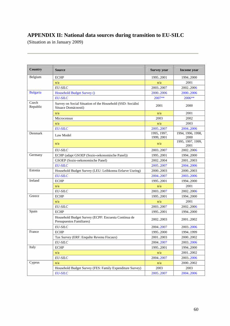
60

APPENDIX II: National data sources during transition to EU-SILC (Situation as in January 2009)

Country Source Survey year Income year

Belgium ECHP 1995..2001 1994..2000 n/a n/a 2001 EU-SILC 2003..2007 2002..2006 Bulgaria Household Budget Survey () 2000..2006 2000..2006 EU-SILC 2007** 2006** Czech Republic

Survey on Social Situation of the Household (SSD: Sociální Situace Domácností)

2001 2000

n/a n/a 2001 Microcensus 2003 2002 n/a n/a 2003 EU-SILC 2005..2007 2004..2006 Denmark

Law Model 1995, 1997, 1999, 2001

1994, 1996, 1998, 2000

n/a n/a

1995, 1997, 1999, 2001

EU-SILC 2003..2007 2002..2006 Germany ECHP (adapt GSOEP (Sozio-oekonomische Panel)) 1995..2001 1994..2000 GSOEP (Sozio-oekonomische Panel) 2002..2004 2001..2003 EU-SILC 2005..2007 2004..2006 Estonia Household Budget Survey (LEU: Leibkonna Eelarve Uuring) 2000..2003 2000..2003 EU-SILC 2004..2007 2003..2006 Ireland ECHP 1995..2001 1994..2000 n/a n/a 2001 EU-SILC 2003..2007 2002..2006 Greece ECHP 1995..2001 1994..2000 n/a n/a 2001 EU-SILC 2003..2007 2002..2006 Spain ECHP 1995..2001 1994..2000 Household Budget Survey (ECPF: Encuesta Continua de

Presupuestos Familiares) 2002..2003 2001..2002

EU-SILC 2004..2007 2003..2006 France ECHP 1995..2000 1994..1999 Tax Survey (ERF: Enquête Revenu Fiscaux) 2001..2003 2000..2002 EU-SILC 2004..2007 2003..2006 Italy ECHP 1995..2001 1994..2000 n/a n/a 2001..2002 EU-SILC 2004..2007 2003..2006 Cyprus n/a n/a 2000..2002 Household Budget Survey (FES: Family Expenditure Survey) 2003 2003 EU-SILC 2005..2007 2004..2006

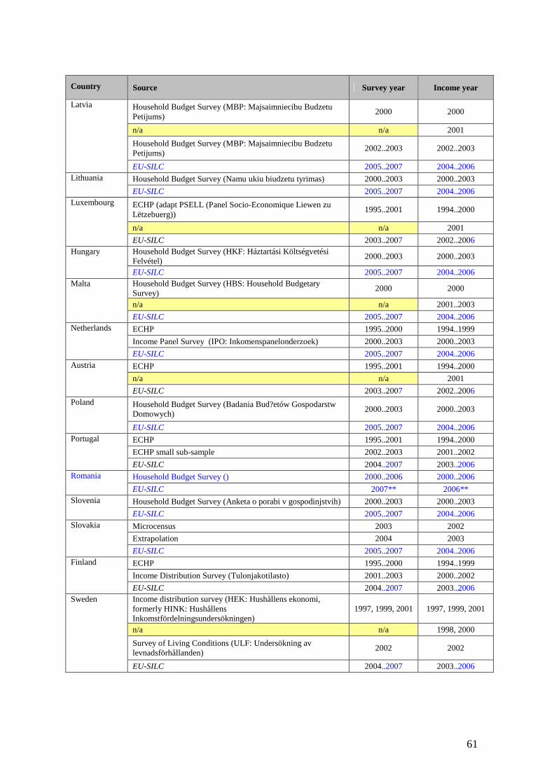
61


Latvia Household Budget Survey (MBP: Majsaimniecibu Budzetu Petijums)

2000 2000

n/a n/a 2001 Household Budget Survey (MBP: Majsaimniecibu Budzetu

Petijums) 2002..2003 2002..2003

EU-SILC 2005..2007 2004..2006 Lithuania Household Budget Survey (Namu ukiu biudzetu tyrimas) 2000..2003 2000..2003 EU-SILC 2005..2007 2004..2006 Luxembourg ECHP (adapt PSELL (Panel Socio-Economique Liewen zu

Lëtzebuerg)) 1995..2001 1994..2000

n/a n/a 2001 EU-SILC 2003..2007 2002..2006 Hungary Household Budget Survey (HKF: Háztartási Költségvetési

Felvétel) 2000..2003 2000..2003

EU-SILC 2005..2007 2004..2006 Malta Household Budget Survey (HBS: Household Budgetary

Survey) 2000 2000

n/a n/a 2001..2003 EU-SILC 2005..2007 2004..2006 Netherlands ECHP 1995..2000 1994..1999 Income Panel Survey (IPO: Inkomenspanelonderzoek) 2000..2003 2000..2003 EU-SILC 2005..2007 2004..2006 Austria ECHP 1995..2001 1994..2000 n/a n/a 2001 EU-SILC 2003..2007 2002..2006 Poland Household Budget Survey (Badania Bud?etów Gospodarstw

Domowych) 2000..2003 2000..2003

EU-SILC 2005..2007 2004..2006 Portugal ECHP 1995..2001 1994..2000 ECHP small sub-sample 2002..2003 2001..2002 EU-SILC 2004..2007 2003..2006 Romania Household Budget Survey () 2000..2006 2000..2006 EU-SILC 2007** 2006** Slovenia Household Budget Survey (Anketa o porabi v gospodinjstvih) 2000..2003 2000..2003 EU-SILC 2005..2007 2004..2006 Slovakia Microcensus 2003 2002 Extrapolation 2004 2003 EU-SILC 2005..2007 2004..2006 Finland ECHP 1995..2000 1994..1999 Income Distribution Survey (Tulonjakotilasto) 2001..2003 2000..2002 EU-SILC 2004..2007 2003..2006 Sweden Income distribution survey (HEK: Hushållens ekonomi,

formerly HINK: Hushållens Inkomstfördelningsundersökningen)

1997, 1999, 2001 1997, 1999, 2001

n/a n/a 1998, 2000 Survey of Living Conditions (ULF: Undersökning av

levnadsförhållanden) 2002 2002

EU-SILC 2004..2007 2003..2006

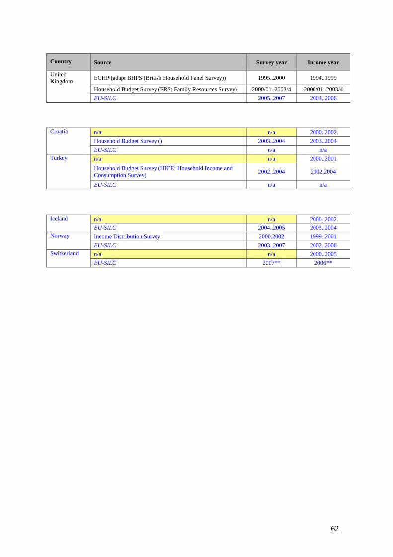
62


United Kingdom

ECHP (adapt BHPS (British Household Panel Survey)) 1995..2000 1994..1999

Household Budget Survey (FRS: Family Resources Survey) 2000/01..2003/4 2000/01..2003/4 EU-SILC 2005..2007 2004..2006 Croatia n/a n/a 2000..2002 Household Budget Survey () 2003..2004 2003..2004 EU-SILC n/a n/a Turkey n/a n/a 2000..2001 Household Budget Survey (HICE: Household Income and

Consumption Survey) 2002..2004 2002.2004

EU-SILC n/a n/a Iceland n/a n/a 2000..2002 EU-SILC 2004..2005 2003..2004 Norway Income Distribution Survey 2000.2002 1999..2001 EU-SILC 2003..2007 2002..2006 Switzerland n/a n/a 2000..2005 EU-SILC 2007** 2006**

Documents

WORKING GROUP STATISTICS ON LIVING CONDITIONS 9-11 …