The Determinants of Non-

residential Real Estate

Values with Special

Reference to Local

Environmental Goods

Sofia F. Franco W. Bowman Cutter

Working Paper

# 603

2016

1

The Determinants of Non-residential Real Estate Values with Special Reference to Local

Environmental Goods

Sofia F. Franco1 W. Bowman Cutter2

May 10th 2016

Abstract

This paper presents the results of an empirical study of the determinants of non-residential real estate values

in Los Angeles County. The data base consists of 13, 370 property transactions from 1996 to 2005. Separate spatial

econometric models are developed for industrial, commercial, retail and office properties. The study focus on the

impact on property values of local amenities.

Our analytical results provide insights on how amenities may affect non-residential properties values and how

the impact may differ across property types. Our empirical results offer evidence that explicitly modeling spatial

dependence is necessary for hedonic non-residential property models where there is interest in local amenities. We

also show that it is also important to account for the temporal dimension since ignoring it can lead to

misinterpretation of the real measure of spatial dependence over time. Moreover, we find that in general amenities

that are jointly valuable to firms and household, such as parks or air quality have either weak or non-robust effects

on nonresidential values. However, the fact that the joint amenities coastal access and crime appear to have stable

correlations across specifications would be consistent with a higher firm than household valuation. In contrast,

those amenities that are likely only valued by firms, such as transportation access and proximity to concentrations

of skilled workers have robust and significant correlations with non-residential values.

JEL Codes: R52, H23.

Keywords: Non-residential Property Values, Local Environmental Amenities, Spatial Econometrics

1 Corresponding Author. Universidade Nova de Lisboa, Nova School of Business and Economics (NovaSBE)

and UECE- Research Unit on Complexity and Economics, ISEG-UTL, Lisboa, Portugal Address: Nova School of

Business and Economics, Campus de Campolide,1099-032, Lisboa, Portugal. Email sfranco@novasbe.pt. Phone

Number: + (351) 213801600. Dr. Franco greatly acknowledges the financial support by FCT (Fundação para a

Ciência e a Tecnologia), Portugal. This article is part of project PTDC/IIM-ECO/4546/2014. 2Pomona College, Department of Economics, Claremont, CA 91711; Telephone 909-607-8187; Email

Bowman.Cutter@Pomona.edu.

2

1. Introduction

The economic literature has exhaustively studied the influence on housing prices of environmental

goods including air quality (Bayer et al. 2009, Kim et al. 2003, Chay and Greenstone 2005, Bockstael

and McConnell 2007), views (Rodriguez and Sirmans 1994, Seiler et al. 2001, Bond et al. 2002), crime

(Pope 2008, Grove 2008), urban forests (Tyrvainem and Miettinen 2000, Mansfield et al. 2005), water

quality (Leggett and Bockstael 2000), proximity to hazards (Bin and Polasky 2004), and many other

factors. By decomposing residential prices into their relevant components, this literature is able to reveal

the amount by which households value the environmental amenities and disamenities being studied.

The commercial real estate sector is also a large part of the national economy, with an estimated $11

trillion value as of the end of 2009 (Florance et al. 2010). However, there are very few studies that have

estimated the influence of amenities or disamenities on the value of non-residential properties. This is

quite surprising because it is likely that these two markets are strongly linked. Offices, commercial and

industrial properties compete for space with residential properties, and the wages firms can offer are

influenced by this competition. Diamond (2012) suggests that firms seek to locate in metropolitan areas

that have high concentrations of skilled workers. If that is a factor driving inter-metropolitan firm

location, should it also not be a factor driving intra-metropolitan migration?

Moreover, temperature, humidity, wind, cloud cover and precipitation also determine how much

energy it takes to keep interior spaces lit and at comfortable temperatures and therefore, impact firms’

cost structure. If in fact, firms observe and capitalize these types of amenities, hedonic methods can be

used to measure the price premium for such attributes, representing the valuation of the marginal buyer.

However, it is unclear how these amenities will be valued in equilibrium where both firms and

households compete for desirable locations. One goal of this paper is to develop such a model.

While there is already valuable work that identifies appropriate environmental indicators for built

non-residential assets, these studies focus on the design and building construction (see for example

Eichholtz et al. 2013) and lesser consideration has been given to the impacts of local public goods such

as crime, presence of skilled workers, weather, air pollution or alternative forms of open space on rents

and selling prices of non-residential properties.

The goal of this paper is therefore to understand how non-residential property values correlate to

local amenities using data on office, commercial, industrial and retail property sales from Los Angeles

County.

The theoretical urban equilibrium model we develop shows that amenities that influence either

commercial or residential property prices will influence the prices and development of both types of

property. In addition, it provides a rigorous theoretical foundation for variable choice and for the control

3

of spatial and temporal dependence in properties valuations in our empirical model of non-residential

property prices.

The empirical portion of this paper seeks to test the predictions of the theoretical model by measuring

how key neighborhood or geographical characteristics are related to non-residential property prices. In

addition, it also investigates whether spatial and temporal dependences should be accounted for in all

sub-sectors of the non-residential market, namely retail, office and industrial. Spatial dependence

implies that high (low) priced real estate assets tend to cluster in some locations (Anselin and Bera

1998).3 This is particular relevant since not accounting for spatial autocorrelation (or spatial dependence)

in presence of spatial interactions in the non-residential real estate market may lead to mispricing of not

only building attributes but also of local amenities. The degree of cross section dependence is usually

calibrated by means of a weighting matrix, where weights can be based on alternatives forms of

contiguity, distance, square distance or the number of nearest neighbors. The spatial weight matrix

captures how two properties are spatially connected to one another at one point in time. However, the

values for each property are also likely to be correlated with each other over time.

While it is likely that spatially close past property values influence current property values, it is

unlikely that spatially close future and unknown property values influence present values. Therefore, the

spatial weights matrix needs to be adjusted for potential temporal influence on the spatial spillover

impacts in a temporal context. Ignoring such temporal dimension in constructing the weights matrix

could lead to misinterpretations on the real measure of spatial dependence over time, which in turn has

implications for the influence of local amenities on property values (Dube and Legros 2013, 2015).

We first run a hedonic model as a benchmark against which we will compare the subsequent model

specifications. Then we employ spatial econometric models that employ spatial and spatio-temporal

weights matrices. These models are applied to 13, 370 non-residential property transactions in Los

Angeles County from 1996 to 2005. Given its multimodal structure, heterogeneity across nodes,

surrounding jurisdictions and environmental amenities, Los Angeles County provides an appropriate

spatial setting to illustrate the theory developed in our theoretical session.

Sivitanidou (1995) and Sivitanidou and Sivitanides (1995) are the most complete papers in the non-

residential rents literature. These papers include a number of geographic and workforce attributes.

However, the less-advanced geographical software of the time did not allow those authors to be as

3 In real estate markets, due to herd behavior of buyers and sellers, the value of a property generally guides price

expectations in a neighborhood (Hott and Monnin 2008, Hott 2012). Furthermore, neighborhoods tend to develop

at the same time and may have similar structural characteristics, such as dwelling size, vintage, interior and exterior

design features (Basu and Thibodeau 1998). Nearby buildings tend also to share the same local amenities like

accessibility, environmental characteristics, and have similar access to labor markets and public facilities.

4

geographically specific as our paper. In addition, we include many green and infrastructure amenities

that those authors likely lacked. Finally, we use a spatial econometric estimator to capture spatial

correlation in both the dependent variable (property prices) as well as in unobservables (residuals). We

also construct a spatio-temporal weights matrix, following Dube and Legros (2013, 2015) methodology,

to evaluate spatial dependence in a context of spatial data (cross-section) pooled over time.4

The sources of non-residential real estate value are interesting in their own right, but our research

also sheds light on the literature on quality of life and intra-city productivity divergence. The current

work on quality of life and city productivity divergence (Diamond 2012, Albouy 2012) tends to assume

that metropolitan areas (MSAs) are spatially uniform and stresses differences between MSAs. However,

MSAs can be quite large and there is likely to be significant intra-MSA differences in productivity and

quality of life. Diamond 2012, especially, posits a dynamic cycle where skill agglomeration increases

productivity, attracting business, which attracts more skilled employees and increases productivity

further. Also, the critical mass of skilled employees creates a market for shopping and entertainment

that also draws more skilled workers. This story contains the hypothesis that firms should locate near

concentrations of skilled workers, which we test in the empirical portion of our paper. We also test

whether firms value proximity to restaurants and shopping.

Our empirical results indicate the importance of controlling for spatial dependence in estimating the

determinants of non-residential values. Spatial parameters are generally statistically significant, and our

simulations indicate that non-spatial estimates of amenity elasticities vary from those generated by

spatial regressions. However, similar to Dube and Legros (2013, 2015), we also find that ignoring the

temporal dimension in constructing the weights matrix leads to misinterpretations on the real measure

of spatial dependence over time. In particular, our results suggest that, for the Los Angeles market,

accounting for spatial-temporal dependence in the lagged dependent variable (sale prices), does not seem

to attenuate the effects of hedonic attributes statistically or economically.

Regarding the impacts of local amenities, we find that in general amenities that are jointly valuable

to firms and household, such as parks or air quality have either weak or non-robust effects on non-

residential values. However, the fact that the joint amenities coastal access and crime appear to have

4 Note that panel data consists of the same unit observed over time, while pooled cross-section data consists of a

different unit observed over time, so that a unit is only observed once or very infrequently. Spatial, or cross-

sectional, databases pooled over time can represent for example real estate sale prices, business opening

(or)/closings, crime location or innovation. For these databases, the panel procedures cannot be applied because a

given spatial observation (located at a point) is only observed once over time. However, Dube and Legros (2013,

2015) clearly show that neglecting the temporal dimension of the data generating process of spatial data pooled

over time can generate biases on the autoregressive coefficient as well as on the coefficient related to the

independent variable which can lead to erroneous interpretation of the indirect and total marginal effect related to

spatial characterization.

5

stable correlations across specifications would be consistent with a higher firm than household valuation.

In contrast, those amenities that are likely only valued by firms, such as transportation access and

proximity to concentrations of skilled workers have robust and significant correlations with non-

residential values. Our results are thus aligned with those of Gabriel and Rosenthal (2004), suggesting

that households and firms value differently local amenities. For this reason, cities or MSAs that are

attractive to firms may be unattractive to households, and vice-versa.

We begin the remaining portion of our paper by examining the literature concerning the determinants

of non-residential rents and values and the related quality of life and quality of the business environment

literature. In section 3 we develop a model of the joint determination of non-residential and residential

rents and values that include the role of amenities and herding behavior by the market participants

followed by comparative static analysis in section 4. Section 5 describes the empirical framework and

the econometric model of non-residential values that includes amenities and spatial and temporal

dependences and auto-correlation. It also discusses the data, which represents a unique combination of

non-residential property transaction data with detailed information on building attributes and local

natural and man-made environmental and urban amenities. Section 6 provides the main empirical results

and finally, section 7 offers conclusions.

2. Literature Review

Application of the hedonic method to the non-residential property (office, commercial, office)

market is recent compared to the housing market and, as a result, references are much fewer. This is

primarily explained by the difficulty of collecting the necessary databases, as description of properties

by their characteristics is generally less reliable for retail, office-commercial and industrial real estate

and warehouses than for housing. However, the improvement in information quality since the 1990s has

encouraged development of this type of work, which for the time being still covers only a limited number

of geographical markets and has focused mostly on office-commercial real estate properties.

The most comprehensive studies of urban spatial variations in non-residential rents are by

Sivitanidou (1995) and Sivitanidou and Sivitanides (1995). Both studies provide a framework for

empirically analyzing location demand and supply-side influences on non-residential rents within

multimodal MSAs. Coupled with a set of firm amenities reflecting traditional demand-side influences

(access to CBD, freeway and airport) and a set of worker amenities (education, crime, access to shopping

opportunities and distance to the ocean), supply-side factors such as local institutional controls were

found in Sivitanidou (1995) to play an important role in shaping variations across space in office-

commercial rents in Greater Los Angeles. A similar conclusion was also reached in Sivitanidou and

Sivitanides (1995). In particular, the study concluded that although firm amenities induced the strongest

6

price effect, worker amenities and zoning constraints also played an important role in industrial pricing

in Greater Los Angeles. While these studies provide important insights of the role these factors play in

shaping intra-urban variations in business rents, they lack hedonic spatial techniques in their estimations

and therefore, do not account for spatial heterogeneity and spatial autocorrelation.

In general, existing empirical studies on the determinants of office-commercial rents have provided

consistent results on the contribution of various locational (distance from city center or distance from

nearest highway interchange) and structural (such as total building square feet, age, height, occupancy,

parking) variables to the spatial variation of office rents. Examples include Brennan et al. (1984) and

Mills (1992) for Chicago, Sivitanidou (1995) for Los Angeles, Bollinger et al. (1998) for Atlanta, Dunse

and Jones (1998) on the market in Glasgow and Nagai et al. (2000) for central Tokyo.

Some studies focus on a specific aspect of rent determinants: architectural features of the buildings

(Doiron et al. 1992, Hough and Kratz 1983), vacancy rate (Frew and Jud 1988; Wheaton and Torto 1988;

Sivitanides 1997), access to main and secondary CBD centers (Bollinger et al. 1998, Sivitanidou 1995),

or proximity to light rail transit and highway systems (Ryan 2005). More recently, studies have measured

the effect of environmental certification on office-commercial (Eichholtz et al. 2010, Miller et al. 2008,

Fuerst and McAllister 2011a,b,c) and industrial warehouse (Harrison and Seiler 2011) rents. Recognition

of the adverse effects of urban sprawl and a heightened awareness of environmental concerns has

contributed to the growth of the green building design and construction movement in the United States.

Yet, none of the previous studies have examined the relative contribution of urban green spaces and

environmental quality (such as levels of air pollution) to the spatial variation in non-residential rents

within multimodal metropolises. It is nevertheless possible that the observed ripple effect of nearby open

space, landscape scenery and air pollution on residential properties may also apply to retail and office

sites.

The hedonic price approach has long been used to quantify the impact of open space on residential

property value, including urban parks and golf courses (Bolitzer and Netusil 2000, Lutzenhiser and

Netusil 2001). A common finding in these studies is that green spaces of these types have positive

impacts on residential property values up to a distance of one-quarter to one-half mile. As much as 3%

of the value of properties could be attributed to park proximity, while proximity to golf courses increased

surrounding property values as much as 21%. There is also empirical evidence that increasing the

amount of water and grassy land covers in views result in increased home sale prices (Sander and

Polasky 2009). For a review on published articles that have attempted to estimate the value of different

types of open space see McConnell and Walls (2005). Bockstael and McConnell (2007), in a review of

wage studies, also find clear evidence that households are willing to give up wages to live in cleaner

7

locations. Thus higher residential rents and lower wages do not represent a higher “cost of living” in the

nice locations but rather a higher “benefit of living” there.

In fact, when amenities have little or no effect on firm costs, either real-estate prices or incomes can

be used as an indicator of quality of life from the households’ point of view. Several studies have

computed quality-of-life rankings for cities, urban counties and metropolitan areas by running two

hedonic equations: one relating housing prices to different amenity variables (such as precipitation,

temperature measures, sunshine, coastal access, crime, air and water pollution) as well as to housing

characteristics; and the other relating incomes for individual households to the amenity levels and

workers’ characteristics. Examples of such studies include Hoehn et al (1987), Blomquist et al. (1988),

Gabriel and Rosenthal (2004), Albouy (2012). However, since the connections between quality of life

and real-estate prices and incomes can be ambiguous when firms costs are strongly linked to amenities,

neither of these variables can be generally used with confidence as an unambiguous indicator of quality

of life. Given all the interdependencies between amenities and households, firms and real-estate

developers decisions, it is possible that both hedonic price and wage regressions yield reverse results

even if these effects are theoretical possible.5

On the other hand, since amenities also affect firms, the empirical procedure used in quality-of-life

studies can also be used to rank cities, counties or metropolitan areas from the perspective of firms. For

example, Rosenthal and Gabriel (2004) have performed an empirical exercise similar to the procedure

used in papers generating quality-of-life rankings. Their study found that the ranking of cities by firms

is very different from the ranking by households, consistent with the different goals of the two groups,

suggesting that the effects of amenities on consumer utilities and firm profits are often not in the same

direction. This in turn suggests that firms and households may also not value environmental amenities

and/or environmental quality the same way. Yet, no studies so far have examined the impact of

alternative environmental amenities and environmental quality on non-residential real estate values and

rents.

3. The Model

This section develops the theoretical underpinnings of the paper. Our framework builds on the model

developed by Sivitanidou (1995) and Hott (2012) in order to analyze the effects of local amenities on

5 For example, in the housing-price regression of Blomquist et al. (1988), better public safety leads to lower rather

than higher housing prices and in the hedonic wage regression higher particulate pollution reduces rather than

increases income.

8

non-residential real estate values.6 By accounting for firm, worker, floor-space and land market

equilibriums, our modeling scheme justifies the inclusion in the non-residential hedonic price function

of not only productivity-enhancing firm amenities, but also utility-bearing worker amenities and land

supply restrictions. In addition, by accounting for herd behavior of the market participants in the sense

that the value of a property generally signals or guides price expectations in a neighborhood, our

theoretical model justifies the inclusion of a spatial lag in our model specification. Finally, because

neighborhood and accessibility attributes of a property are not always directly observable and sources

of spatial autocorrelation in property prices also include measurement errors, unsuitable functional form

and model misspecification, spatially correlated errors in hedonic model may result, which in turn

require a specific statistical approach.

3.1. Assumptions

Let’s assume our county contains many cities, indexed by j . Cities differ in two types of attributes:

natural and artificial amenities and land-use regulations.

Some amenities (e.g. costal proximity) directly affect households’ utility, while others (good

transportation access facilitating trips within or out of the city or agglomeration economies) directly

affect firms’ productivity or transportation costs. Other amenities (e.g. climate conditions and public

safety) may affect both the location of firms and households. Let HjA represent a vector of amenities in

city j that directly affect households’ utility and FjA is a vector of amenities in city j affecting firms’

productivity and production.

Each city has two zoning methods to control land use: a restriction on the quantity of land available

for a certain use and a set of regulations on office-commercial construction.

Land within each city is homogenous. Capital is costless mobile across cities, and is paid the price

i everywhere. Office-floor space is owned by absentee landlords who rent the space to local firms. Land

is owned by absentee landowners who rent the land to local residents and local developers. Households

are perfectly mobile, have identical tastes and skills, and each supply a single unit of labor. Office-

commercial firms are also perfectly mobile and identical. All factors are fully employed and both output

and input markets are competitive.

A long-run equilibrium requires that land, labor, and floor space markets be cleared simultaneously

through appropriate rent and wage adjustments. Residential land rents ( HjP ), office-commercial land

6 Hott (2012) model takes into account that a house can be seen as an asset which price should reflect a risk-return

tradeoff but also as a good which price should reflect the utility gain from owning it.

9

rents ( FjP ), firm floor space rents ( FjR ), labor wages ( jw ), number of households/workers demanded

by each firm ( jN ) and number of firms ( jF ), are endogenous. The equilibrium conditions in the model’s

various markets are discussed below.

3.2. Households Equilibrium

Households have preferences over residential land, h , a numeraire nonland good, z , and a set of

households’ amenities HjA .7 At each city, a household solves the following utility maximization

problem:

0

,

..

),(max);,(

wwzhPts

AzhUAPwV

jHj

Hjzh

HjHjj

(1)

where )(U is concave over h and z and increasing in HjA , HjP is the rental expenses on residential

land per unit of land and jw is wage in city j . The nonlabor income 0w is assumed to be independent

of location and will be suppressed in the model henceforth. For simplicity, we assume that the price of

the numeraire good is set to 1. The solution of (1) yields the demand functions for residential land and

the nonhousing good as

),( Hjjd Pwh (2)

)( jwz (3)

where 0dw j

h , 0dPHj

h .8

The indirect utility function );,( HjHjj APwV gives the maximum utility achieved in city j given the

wage, the residential land price and the level of households’ amenities. Households choose residential

locations to maximize );,( HjHjj APwV by considering the trade-offs between wage, residential land

rents and households’ amenities. Since households are fully mobile, their utility must be the same across

all the cities that they inhabit. Therefore, equilibrium for households requires that wages and residential

land rents adjust to equalize utility in all cities:

VAPwAPwV HjHjjHjHjj ),();,( (4)

7 Spatial variations in nonhousing costs, which are smaller than spatial variations in housing costs, are ignored in

this analysis. 8 Note that because HjA is separable in the utility function, (2) and (3) do not depend directly on the city’s

households’ amenities.

10

where V is the exogenous uniform utility level and (.) is a function that satisfies 0wj and 0HjP

. Therefore, 0wjV , 0HjAV and 0

HjPV .

If there are SjN households/workers in city j , then total demand for residential land is given by

),( HjjdS

j PwhN . (5)

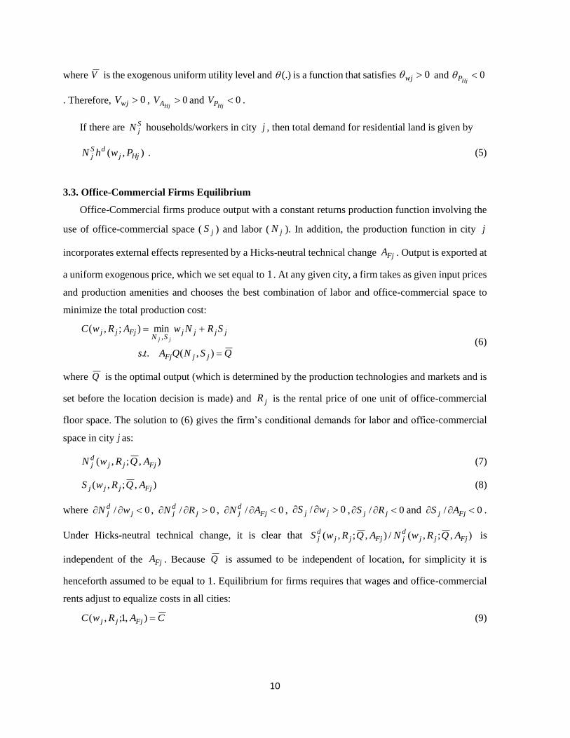
3.3. Office-Commercial Firms Equilibrium

Office-Commercial firms produce output with a constant returns production function involving the

use of office-commercial space ( jS ) and labor ( jN ). In addition, the production function in city j

incorporates external effects represented by a Hicks-neutral technical change FjA . Output is exported at

a uniform exogenous price, which we set equal to 1 . At any given city, a firm takes as given input prices

and production amenities and chooses the best combination of labor and office-commercial space to

minimize the total production cost:

QSNQAts

SRNwARwC

jjFj

jjjjSN

Fjjjjj

),(..

min);,(,

(6)

where Q is the optimal output (which is determined by the production technologies and markets and is

set before the location decision is made) and jR is the rental price of one unit of office-commercial

floor space. The solution to (6) gives the firm’s conditional demands for labor and office-commercial

space in city j as:

),;,( Fjjjdj AQRwN (7)

),;,( Fjjjj AQRwS (8)

where 0/ jdj wN , 0/ j

dj RN , 0/ Fj

dj AN , 0/ jj wS , 0/ jj RS and 0/ Fjj AS .

Under Hicks-neutral technical change, it is clear that ),;,(/),;,( FjjjdjFjjj

dj AQRwNAQRwS is

independent of the FjA . Because Q is assumed to be independent of location, for simplicity it is

henceforth assumed to be equal to 1. Equilibrium for firms requires that wages and office-commercial

rents adjust to equalize costs in all cities:

CARwC Fjjj ),1;,( (9)

11

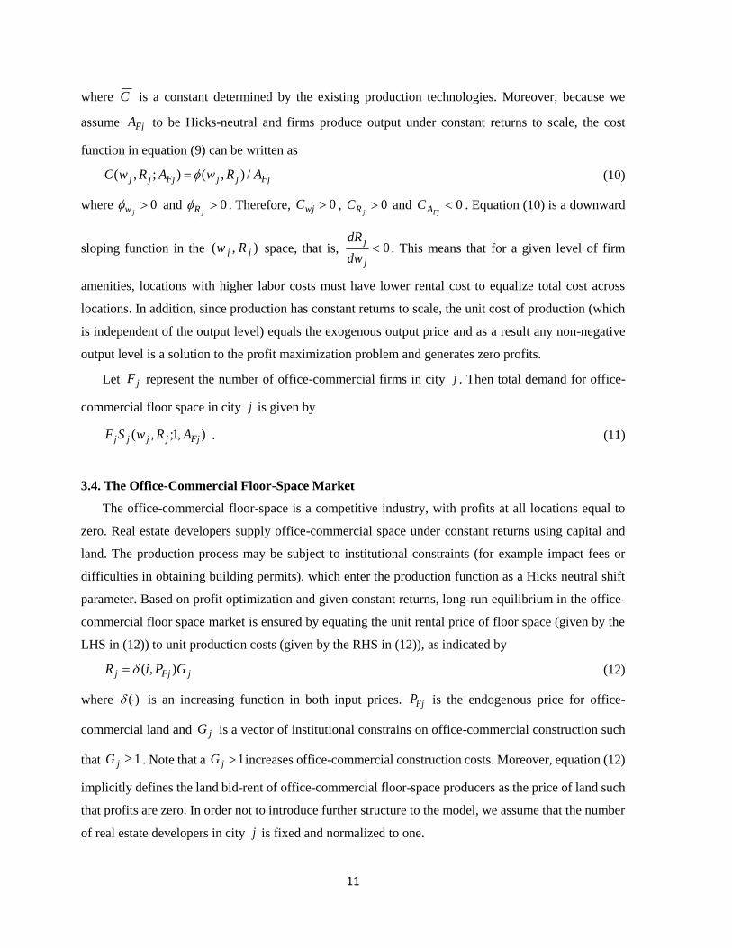
where C is a constant determined by the existing production technologies. Moreover, because we

assume FjA to be Hicks-neutral and firms produce output under constant returns to scale, the cost

function in equation (9) can be written as

FjjjFjjj ARwARwC /),();,( (10)

where 0jw and 0

jR . Therefore, 0wjC , 0jRC and 0

FjAC . Equation (10) is a downward

sloping function in the ),( jj Rw space, that is, 0j

j

dw

dR. This means that for a given level of firm

amenities, locations with higher labor costs must have lower rental cost to equalize total cost across

locations. In addition, since production has constant returns to scale, the unit cost of production (which

is independent of the output level) equals the exogenous output price and as a result any non-negative

output level is a solution to the profit maximization problem and generates zero profits.

Let jF represent the number of office-commercial firms in city j . Then total demand for office-

commercial floor space in city j is given by

),1;,( Fjjjjj ARwSF . (11)

3.4. The Office-Commercial Floor-Space Market

The office-commercial floor-space is a competitive industry, with profits at all locations equal to

zero. Real estate developers supply office-commercial space under constant returns using capital and

land. The production process may be subject to institutional constraints (for example impact fees or

difficulties in obtaining building permits), which enter the production function as a Hicks neutral shift

parameter. Based on profit optimization and given constant returns, long-run equilibrium in the office-

commercial floor space market is ensured by equating the unit rental price of floor space (given by the

LHS in (12)) to unit production costs (given by the RHS in (12)), as indicated by

jFjj GPiR ),( (12)

where )( is an increasing function in both input prices. FjP is the endogenous price for office-

commercial land and jG is a vector of institutional constrains on office-commercial construction such

that 1jG . Note that a 1jG increases office-commercial construction costs. Moreover, equation (12)

implicitly defines the land bid-rent of office-commercial floor-space producers as the price of land such

that profits are zero. In order not to introduce further structure to the model, we assume that the number

of real estate developers in city j is fixed and normalized to one.

12

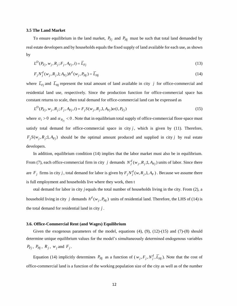
3.5 The Land Market

To ensure equilibrium in the land market, FjP and HjP must be such that total land demanded by

real estate developers and by households equals the fixed supply of land available for each use, as shown

by

FjFjjjjFjD LiAFRwPL ),,;,,( (13)

HjHjjd

Fjjjdjj LPwhARwNF ),();1,,( (14)

where FjL and HjL represent the total amount of land available in city j for office-commercial and

residential land use, respectively. Since the production function for office-commercial space has

constant returns to scale, then total demand for office-commercial land can be expressed as

),(),1,,(),,;,,( FjFjjjjFjjjjFjD PiARwSFiAFRwPL (15)

where 0i and 0FjP . Note that in equilibrium total supply of office-commercial floor-space must

satisfy total demand for office-commercial space in city j , which is given by (11). Therefore,

),1;,( Fjjjj ARwSF should be the optimal amount produced and supplied in city j by real estate

developers.

In addition, equilibrium condition (14) implies that the labor market must also be in equilibrium.

From (7), each office-commercial firm in city j demands ),1;,( Fjjjdj ARwN units of labor. Since there

are jF firms in city j , total demand for labor is given by ),1,,( Fjdjj ARwNF . Because we assume there

is full employment and households live where they work, then t

otal demand for labor in city j equals the total number of households living in the city. From (2), a

household living in city j demands ),( Hjjd Pwh units of residential land. Therefore, the LHS of (14) is

the total demand for residential land in city j .

3.6. Office-Commercial Rent (and Wages) Equilibrium

Given the exogenous parameters of the model, equations (4), (9), (12)-(15) and (7)-(8) should

determine unique equilibrium values for the model’s simultaneously determined endogenous variables

FjP , HjP , jR , jw and jF .

Equation (14) implicitly determines HjP as a function of ( Hjdjjj LNFw ,,, ). Note that the cost of

office-commercial land is a function of the working population size of the city as well as of the number

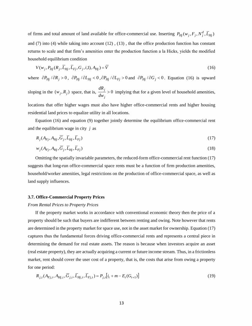
13

of firms and total amount of land available for office-commercial use. Inserting ),,,( HjdjjjHj LNFwP

and (7) into (4) while taking into account (12) , (13) , that the office production function has constant

returns to scale and that firm’s amenities enter the production function a la Hicks, yields the modified

household equilibrium condition

VAiGLLRPwV HjjFjHjjHjj )),1,,,,,(,( (16)

where 0/ jHj RP , 0/ HjHj LP , 0/ FjHj LP and 0/ jHj GP . Equation (16) is upward

sloping in the ),( jj Rw space, that is, 0j

j

dw

dR implying that for a given level of household amenities,

locations that offer higher wages must also have higher office-commercial rents and higher housing

residential land prices to equalize utility in all locations.

Equation (16) and equation (9) together jointly determine the equilibrium office-commercial rent

and the equilibrium wage in city j as

),,,,( FjHjjHjFjj LLGAAR (17)

),,,,( FjHjjHjFjj LLGAAw (18)

Omitting the spatially invariable parameters, the reduced-form office-commercial rent function (17)

suggests that long-run office-commercial space rents must be a function of firm production amenities,

household/worker amenities, legal restrictions on the production of office-commercial space, as well as

land supply influences.

3.7. Office-Commercial Property Prices

From Rental Prices to Property Prices

If the property market works in accordance with conventional economic theory then the price of a

property should be such that buyers are indifferent between renting and owing. Note however that rents

are determined in the property market for space use, not in the asset market for ownership. Equation (17)

captures thus the fundamental forces driving office-commercial rents and represents a central piece in

determining the demand for real estate assets. The reason is because when investors acquire an asset

(real estate property), they are actually acquiring a current or future income stream. Thus, in a frictionless

market, rent should cover the user cost of a property, that is, the costs that arise from owing a property

for one period:

)(),,,,( 1,,,,,,, ttttjtFjtHjtjtHjtFjtj GEmiPLLGAAR (19)

14

where tjP , is the property price j at time t , ti is the real interest rate, m is the constant maintenance

rate and )( 1tt GE is the expected capital gains defined as

tj

tjtjttt

P

PPEdGE

,

,1,1

])()1[()(

(20)

where d is the constant depreciation rate.

Inserting (20) into (19) yields, after some manipulations, the following property price equation:

mi

PEdRP

t

tjttjtj

1

)()1( 1,,, . (21)

Herding Behavior

We now introduce herding behavior by assuming that rational but imperfectly informed investors

learn from the decisions of the other investors. In particular, let’s assume that investor j expectations

regarding the future property price depends on both social and non-social signals. Informational

influence affects expectations of real estate price appreciation if investors look to others in deciding

whether or not their real estate purchase will generate capital appreciation. In this sense, we can write

the expectation regarding future price as )( 1, jtjt PE , with j representing the information set upon

which investor j bases his expected capital gains and described as follows:

tjjQq

Q

q

jqj Px ,,

1

1

,

(22)

where jq, and jQ, are the weights placed by investor j on the information contained in the non-social

signal qx and social signal tjP , , respectively. It is assumed that 10 , jq , q and 1

1

,

Q

q

jq .

According to (22) the information set has two different components. The first component on the

right-hand-side of (22) captures all currently available objective information relating to non-social

factors ( qx ) such as for example maintenance rate, depreciation rate and interest rates.

The second component on the right-hand-side of (22) contains the social information regarding the

willingness to pay of other owner occupiers for similar properties ( tjQ Px , ). In this sense, our model

captures the idea that a selling price of a property at a particular location acts as a signal that guides the

selling prices of its neighboring properties.

15

If markets are weakly efficient, social signals are ignored (that is 0Q for all investors) and all

investors respond symmetrically to non-social signals so that q is constant across all investors, then

the non-social information is factored into prices to give an unbiased estimate of future prices ( tP ). In

this case the expectation of future price is represented as

t

Q

q

qqjtjt PxPE

)(

1

1

1, (23)

However, when 0Q , social information will distort prices away from their fundamental value.

The action of other investors introduces herd externalities in which the herd’s judgment is biased by

social information about the action of others:

tjQtQ

Q

q

qqjtjt PPxPE ,

1

1, )1()(

. (24)

Representative office-commercial property price for city j at time t

Finally, inserting (24) back into (21) we get the representative office-commercial property price for

city j at time t as

])1[(1

)1(

1

1

])1)[(1(

,,

,,,

tjQtQtt

tj

t

tjQtQtjtj

PPmi

d

mi

R

mi

PPdRP

(25)

with the fundamental value of office-commercial rents, tjR , , given by equation (17). According to (25)

real estate prices can divert from their fundamental value because of a herding behavior. The

fundamental value of office-commercial properties is represented by:

mi

RE

mi

d

mi

RP

mi

d

mi

R

t

tjt

tt

tjt

tt

tj

1

1,,,

11

)1(

11

)1(

1 . (26)

Following (26), the fundamental price of a non-residential real estate property is driven by present

and future office-commercial rents and interest rates. However, the presence of a herding behavior (

0Q ) may create a positive feedback effect between the attractiveness of a real estate property and

its price, ][ , ttjQ PP . If ][ , ttj PP is positive then the excess return from this price externality is

positive, which pushes the price of a real estate property higher. On the other hand if ][ , ttj PP is

negative, the opposite effect occurs. The parameter Q captures the strength of price externality. This

16

in turn suggests that real estate markets are not fully efficient and autocorrelation in price inflation should

be accounted for in studies that examine the determinants of real estate prices.

It is worth pointing out that ][ , ttj PP captures proximity both in space and time because the social

signal tjP , incorporates property prices from spatial neighbors, which in turn incorporate expectations

over future prices.

Equation (25) therefore sets the stage for the empirical analysis of office-commercial property values

and location desirability within Los Angeles County. In section 5.3 we provide details on how we build

our spatio-temporal weights matrix, which specifies the weight by using both the space and time of the

nearest similar transacted property (neighbor). Each row in this matrix pertains to a transaction in our

data set.

4. Comparative Statics

The equilibrium effects of land-use regulations, as well as production and household amenities, can

be derived by totally differentiating (4), (9), (12)-(15) and (7)-(8) with respect to each variable of interest.

Because of all the interdependencies, the comparative statics of this type of model can be fairly complex

and lengthy. The steps for the case where the amenity is beneficial to households but neutral to firms are

shown in the appendix, and the remaining derivations are available on request. In this section, we just

indicate the signs for changes in each exogenous variable and discuss the results.

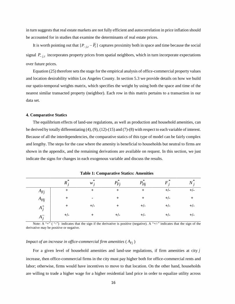
Table 1: Comparative Statics: Amenities

*jR

*jw

*FjP

*HjP

*jF

*jN

FjA + + + + +/- +/-

HjA + - + + +/- +

jA

+ +/- + +/- +/- +/-

jA

+/- + +/- +/- +/- +/-

Note: A “+” ( “-”) indicates that the sign if the derivative is positive (negative). A “+/-” indicates that the sign of the

derivative may be positive or negative.

Impact of an increase in office-commercial firm amenities ( FjA )

For a given level of household amenities and land-use regulations, if firm amenities at city j

increase, then office-commercial firms in the city must pay higher both for office-commercial rents and

labor; otherwise, firms would have incentives to move to that location. On the other hand, households

are willing to trade a higher wage for a higher residential land price in order to equalize utility across

17

cities. In addition, higher office-commercial land prices are established in city j , as more firms bid

higher floor-space rents. However, higher labor and rental costs together with higher productivity have

an ambiguous effect on the number of demanded workers and on the amount of demanded floor space.

As a result, the impact of a change in firms’ amenities on the equilibrium number of workers/households

in city j is ambiguous.

Impact of an increase in household amenities ( HjA )

If, for a given level of firm amenities and regulations, city j becomes more attractive to households,

residential location demand will grow, increasing residential land rents, office commercial land rents as

well as office-commercial rents. Higher office-commercial rents can be afforded by firms, as households

are now willing to accept lower wages in exchange for better amenities. In equilibrium, the number of

hired workers is higher in a location with better worker amenities because higher office-commercial

rents compel firms to demand less floor-space while a lower wage incentives firms to hire more workers.

Thus, and in contrast to the previous case, our model suggests that household amenities have a positive

effect on employment. However, the impact on the equilibrium number of firms is still ambiguous.

Impact of an increase in an amenity that affects both firms and households ( jA )

Some amenities can affect both firms’ costs and households’ welfare. A firm located in a temperate

climate may spend less on heating and cooling for its offices and factories, so that the cost function

would be decreasing in jA . On the other hand, households prefer temperate to extreme climate (too cold

or too hot) so that the indirect utility function is increasing in jA . Let’s assume that amenity jA affects

positively both firms and households. In this case, the equilibrium office-commercial rents and office-

commercial land prices are still higher for the city with better amenity. However, wage and residential

land price can be higher or lower, depending on the relative magnitude of the effects of the amenity on

firms’ costs and households’ utility. If the cost (utility) effect dominates the utility (cost) effect then both

the equilibrium wage and residential land rent are higher (lower).

Now suppose that amenity jA affects positively firms but it is a disamenity for households because

it may for example cause more traffic or pollution. In this case the negative effect of the amenity on

households’ utility reinforces the impact on wages, but offsets the effects on office-commercial rents

and on housing residential land prices. If the disamenity effect dominates, then a city with high firm

amenity and high household disamenity (or low household amenity) may actually have lower office-

18

commercial rents and lower residential land prices. Conversely, if the cost amenity effect dominates,

then a city may have higher office-commercial rents and higher residential land prices.9

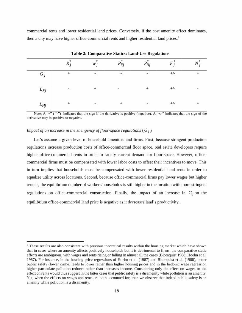
Table 2: Comparative Statics: Land-Use Regulations

*jR

*jw

*FjP

*HjP

*jF

*jN

jG + - - - +/- +

FjL - + -

+ +/- -

HjL + - + - +/- +

Note: A “+” ( “-”) indicates that the sign if the derivative is positive (negative). A “+/-” indicates that the sign of the

derivative may be positive or negative.

Impact of an increase in the stringency of floor-space regulations ( jG )

Let’s assume a given level of household amenities and firms. First, because stringent production

regulations increase production costs of office-commercial floor space, real estate developers require

higher office-commercial rents in order to satisfy current demand for floor-space. However, office-

commercial firms must be compensated with lower labor costs to offset their incentives to move. This

in turn implies that households must be compensated with lower residential land rents in order to

equalize utility across locations. Second, because office-commercial firms pay lower wages but higher

rentals, the equilibrium number of workers/households is still higher in the location with more stringent

regulations on office-commercial construction. Finally, the impact of an increase in jG on the

equilibrium office-commercial land price is negative as it decreases land’s productivity.

9 These results are also consistent with previous theoretical results within the housing market which have shown

that in cases where an amenity affects positively households but it is detrimental to firms, the comparative static

effects are ambiguous, with wages and rents rising or falling in almost all the cases (Blomquist 1988; Hoehn et al.

1987). For instance, in the housing-price regressions of Hoehn et al. (1987) and Blomquist et al. (1988), better

public safety (lower crime) leads to lower rather than higher housing prices and in the hedonic wage regression

higher particulate pollution reduces rather than increases income. Considering only the effect on wages or the

effect on rents would thus suggest in the latter cases that public safety is a disamenity while pollution is an amenity.

Yet, when the effects on wages and rents are both accounted for, then we observe that indeed public safety is an

amenity while pollution is a disamenity.

19

Impact of an increase in the stringency of office-commercial zoning ( FjL )

A lower amount of land designated for office-commercial development must be associated with

higher office-commercial land prices to equalize land demand to the constrained supply. This, in turn,

requires higher office-commercial floor-space rents, and therefore, a lower wage to maintain firm

indifference at the unit production cost. Office-commercial firms are able to pay less for labor since

households are willing to trade lower wages for lower residential land rents to equalize utility to the

exogenous uniform level. As a result, the number of demanded workers in city j by each office-

commercial firm is higher in the new equilibrium.

Impact of an increase in the stringency of residential zoning ( HjL )

On the other hand, a lower amount of land designated for residential development must be associated

with higher residential land prices which require higher wages to keep a current household indifferent

across locations. This leads firms to trade higher labor costs for lower office-commercial rents in order

not to move. The decrease in office-commercial rents then decreases the price of office-commercial land.

From the combined analysis of FjL and HjL , we notice that in the absence of externalities, reducing

the amount of land allowed in a certain use raises the land price of that use but decreases the land price

of the remaining land uses. In addition, the floor-space output associated with the restricted land use

declines while its price rises and the floor-space output price associated with the unrestricted land use

drops. Therefore, allowable use zoning affects land values differently across uses. On the other hand, an

institutional constraint on production raises the floor-space output price associated with the restricted

land use. However, and in contrast to the allowable use zoning, it affects land values equally across land

uses.

5. The Empirical Model

5.1. Hedonic Analysis

The literature for quality-of-life amenities and quality-of-business amenities estimate reduced form

equations of equilibrium wage and housing prices in order to explain how prices vary with amenity

levels across cities. However, our main goal is to examine the determinants of intra-metropolitan

variations in non-residential prices focusing on the role of local amenities. As such, we aim to estimate

the reduce form (25) which includes not only quality-of-life amenities but also productive amenities and

local institutional restrictions as well as a herd behavior around neighboring property prices where price

expectations are formed based on neighboring values.

20

Given its multimodal structure, heterogeneity across nodes, surrounding jurisdictions and

environmental amenities, Los Angeles County provides an appropriate spatial setting to illustrate the

theory developed in session 3. Before describing in some detail the datasets and the variables used in

our empirical exercise, the specific empirical formulation, which builds on the theoretical formulation

in (25) and accounts for the spatial nature of the data available, is discussed. Our model for the hedonic

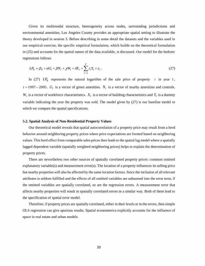
regressions follows

T

t

ittiiiiit YXWNGLP

1

0 . (27)

In (27) itLP represents the natural logarithm of the sale price of property i in year t ,

20051997 t . iG is a vector of green amenities. iN is a vector of nearby amenities and controls.

iW is a vector of workforce characteristics. iX is a vector of building characteristics and tY is a dummy

variable indicating the year the property was sold. The model given by (27) is our baseline model to

which we compare the spatial specifications.

5.2. Spatial Analysis of Non-Residential Property Values

Our theoretical model reveals that spatial autocorrelation of a property price may result from a herd

behavior around neighboring property prices where price expectations are formed based on neighboring

values. This herd effect from comparable sales prices then leads to the spatial lag model where a spatially

lagged dependent variable (spatially weighted neighboring prices) helps to explain the determination of

property prices.

There are nevertheless two other sources of spatially correlated property prices: common omitted

explanatory variable(s) and measurement error(s). The location of a property influences its selling price

but nearby properties will also be affected by the same location factors. Since the inclusion of all relevant

attributes is seldom fulfilled and the effects of all omitted variables are subsumed into the error term, if

the omitted variables are spatially correlated, so are the regression errors. A measurement error that

affects nearby properties will result in spatially correlated errors in a similar way. Both of them lead to

the specification of spatial error model.

Therefore, if property prices are spatially correlated, either in their levels or in the errors, then simple

OLS regression can give spurious results. Spatial econometrics explicitly accounts for the influence of

space in real estate and urban models.

21

5.3. Our Empirical Strategy

Our goal for this paper is to establish whether there are robust associations between various local

amenities and the prices of non-residential properties. We aim to investigate whether there are durable

associations or whether the amenity variables are simply capturing local unobservables. To this end we

run specifications with a number of different sets of controls and combinations of variables and examine

whether there are significant changes in sign and magnitude of the key coefficients.

The properties are classified into several broad property types including offices, industrial

properties, and two types of retail. We hypothesize that office properties should be more sensitive to

green, and neighborhood amenities because high-skill workers have been shown to have greater taste

for these amenities. Production amenities are more mixed. The concentration of high skill workers

should have a positive impact on office prices, but an unknown impact of industrial and retail prices.

Other amenities such as rail access, freeway access, or airport proximity may have impacts on all

property types. Differences in amenity value between the different property types are a signal that the

regressions are capturing correlations between amenities and prices.

Studies focused on characteristics of the property or structure, such as an environmental label, can

use a fixed effects strategy, however, fixed effects will eliminate the influence of the amenities we wish

to examine. Nearby properties are likely to have similar unobservable characteristics and spatial

regression controls for these. We use a spatial method that allows for both spatial autocorrelation and

spatial lag. That is, the specification allows for the errors and the dependent variable to be correlated

across nearby observations.

Spatial Models

Spatial methods have been used sparingly in the non-residential real estate literature, and to our

knowledge they have never been used to examine the relationship between amenities and non-residential

real estate prices. The specification is the same as in (27) except:

ueWLPW 21 (28)

where measures the degree of spatial autocorrelation, 1W is a weighting matrix, LP is the vector of

property prices, is a scalar measuring the degree of spatial error correlation, 2W is another (possibly

distinct) weighting matrix, and e and u are i.i.d disturbances.10

10 In order to test the robustness of our results to alternative specifications of our k-nearest neighbor matrix, we

computed different matrices on the basis of the 8th, 10th, 15th and 30th closest neighbor criteria. While our coefficient

estimates aren't much different between the runs, the spatial dependence declines with the increasing number of

nearest neighbors taken into account. Our final runs are at 10 but with a mile cutoff, which only affects a few

properties but avoided some clusters where properties are very far apart.

22

Using the weights matrix, the lag operator LPW1 captures the spatially weighted average of the

variable of interest in a given location. This is analogous to our theoretical term ][ ,tjP in equation (25).

Thus, the spatial variable captures the impact of the neighboring unit valuations on the transaction price

of a property. One of the innovative features of our spatial model is the construction of an integrated

spatio-temporal weights matrix, following the methodology of Dube and Legros (2013, 2015). This

spatio-temporal weights matrix allows us to incorporate the temporal dimension of the data generating

process of spatial data pooled over time.

Spatio-Temporal Weights Matrices ( 1W and 2W )

Typical spatial econometric methods ignore the influence of time on spatial dependence. However,

with data over eight years the assumption that there is no temporal dimension to spatial autocorrelation

is unlikely to be true. For instance, it is unlikely to be either spatial or error correlation with a property

that is sold several years in the future.

Following Dube and Legros (2013, 2015), we can obtain the spatio-temporal weights matrix (W )

by separating its construction into a spatial ( S ) and temporal (T ) weighting matrices. While S uses an

inverse Euclidean distance function to determine the impact of neighboring transactions based on

geographical proximity and a critical cut-off miles distance, T takes temporal dependence through an

inverse function of the time elapsed between realization of two transactions with cut-offs memory effects

for both future and past transactions. In particular, each element jit , of the temporal matrix T is given

by:

ti, j =

(vi - v j )-g if vi - v j £ vp;"i ¹ j and vi > v j

vi - v j

-g

if vi - v j £ v f ;"i ¹ j and vi < v j

1 if vi = v j

0 otherwise

ì

í

ïïï

î

ïïï

(29)

where iv and jv are the time (quarterly values in our case) when properties i and j are sold

respectively, vp is a cut-off value for past transactions (sales), v f is a cut-off value for future

transactions, and is a parameter that determines how fast observations fade in importance as the

distance in time increases (time fade parameter). We test different values for these parameters with our

data. Since the transactions are ordered chronologically, the lower triangular matrix of T contains actual

and past transactions, while the upper triangular matrix contains actual and future transactions. Finally,

to incorporate the simultaneity of both spatial and temporal relations, we multiply, term by term, the two

23

developed relations matrices S and T , resulting in our spatio-temporal matrix TSW , with the

Hadamard matricial product. We also examined a variety of spatial and temporal weight matrices for

both the error and spatial lag.

If is significant, then the non-spatial estimate will generally be biased. Therefore, it is important

to test for spatial autocorrelation. Not accounting for spatial error correlation does not bias coefficients,

but does result in inefficient estimation. We also examined results across property types and with

different sets of local controls in the spatial framework. If coefficients on amenities in the spatial

regressions are significant in the expected direction and differ across property types in expected ways,

then that is evidence that the amenity coefficients are capturing a real association as opposed to capturing

local unobservables.

5.4. Data and Variables

Parcel-level data on non-residential property sales from 1996 through 2005 over a significant portion

of Los Angeles County was obtained through Costar Group, a national commercial real estate

information provider (www.costar.com). After removing several types of parcels not suitable for the

analysis and data with missing variables we were left with 13,370 observations.11 The database contains

the sales price of each property and a vector of structural characteristics (such as building coverage,

permeable area, building square footage, and parking lot spaces, and property code).

The initial database assigned each observation as one of three general land use types: industrial,

office or retail. We divide properties into 4 classes of non-residential use: (1) industrial, which includes

manufacturing, warehouse, and other industrial uses; (2) Office properties; (3) service retail, which

includes banks, restaurants, various services businesses such as doctor’s offices, and auto related

services; and, (4) mixed and shopping retail, the last includes many small shopping centers with

shopping as well as some service retail storefronts (see Table 3 in the Appendix).12

Our variables come from many different data sets. Tables 4 and 5 in the Appendix detail the variables

and show the summary statistics, respectively.

We look at several types of green amenities including air quality, proximity to parks, wilderness,

and shore, weather, and shore proximity. For air quality, we found that the average level of pollutants

is very similar across all areas of the county. The main difference is in the right tails of the distribution

11 We removed several types of parcels which were not suitable for the analysis, namely parking, public facilities,

residential, heavy industrial, industrial park, pleasure retail, retail-residential, retail-office, hi-rise-office. We also

removed categories where there were few observations and where it was not clear how to group them with other

categories. Also, we dropped observations from 1996 because there were few observations. We also dropped any

repeat sales which were just a few observations to begin with. 12 Light industrial and industrial were combined into industrial and office-residential, office-industrial and lo-rise

office into the office category. Dummy variables for these subcategories are included in all specifications.

24

where unhealthy levels of pollutants occur. Because of this we looked at the 90th and 95th percentiles of

the pollutant distribution as an indication of how often there are unhealthy levels of pollutants. We found

that many of the pollution variables are highly correlated with the Ozone 1-hour measures. We use the

90th percentile of Ozone (translated to the Air Quality Index (AQI)) Ozone1_90 as an indicator for high

levels of several air pollutants. In addition, to capture measures of air pollution that may be more

accessible to the public, we use the number of days above 100 AQI, the level at which air quality is

unhealthy. 13

Weather and temperature are another key green amenity. Our data includes monthly averages for

six different meteorological measures (cooling degree days, heating degree days, maximum temperature,

minimum temperature, precipitation, and relative humidity). We decided to use principal component

analysis because of the large number of variables and the high degree of correlation. Our analysis showed

that two principal components (weathf1 weathf2) capture almost all of the variation from these variables

and so we use the two principal components as our controls for weather.

We also examine proximity to various green features including parks, wilderness, golf courses, and

the shore. Manual inspection of the data indicates that only very nearby parks and wilderness are

accessible or visible from the property. We use as a variable an indicator of whether parks or golf

courses are within .2 miles of the property (respectively regpars20 and golf20). For wilderness, there

are few properties within a short distance so we use an indicator of one mile or less distance, wild01.

Shore proximity is different as employees may value being close to shore even if it is not immediately

accessible. We use a quadratic in distance to the closest shore to capture this amenity. The linear distance

to the shore is d_sea and the quadratic d_sea2.

Zoning designation is thought to be important to building value (Sivitanidou 1995). We obtained

zoning maps of each city and then used GIS to map each property to the cities’ zoning areas. Cities use

a variety of different zoning names (there were over 150 in total for all properties), however the zoning

designation usually allow one or of the following uses: commercial, industrial, office, residential, mixed

use, and special downtown zone.14 We created indicator variables for each of these uses and categorized

13 The AQI is an index that tells how clean or polluted the air is, and what associated health effects might be. EPA

calculates the AQI for five major air pollutants regulated by the Clean Air Act (ground-level ozone, particle

pollution, carbon monoxide, sulfur dioxide, and nitrogen dioxide). An AQI value of 100 generally corresponds to

the national air quality standard for the pollutant, which is the level EPA has set to protect public health. AQI

values below 100 are generally thought of as satisfactory. When AQI values are above 100, air quality is considered

to be unhealthy at first for certain sensitive groups of people, then for everyone as AQI values get higher. 14 The zoning designations frequently distinguish between the types of industrial activity, but the descriptions are

not adequate to distinguish types so we lumped all industrial zoning designation together. We also categorized

any manufacturing as an industrial zone. In addition, there are a variety of residential zones, but we in our data

there are few properties in any one zone so we grouped all residential properties together.

25

the zone by each permissible use in the zoning designation. So, for example, a zone whose description

says that both commercial and industrial uses are permissible would get a one for each use.

Neighborhood amenities such as availability of shopping and retail, distance to highways, distance

to airports, distance to business districts, crime levels and rail access are also included in our model. A

property with access to these amenities might be more valuable because of its ability to attract skilled

workers, customers, or boost productivity. Much of the previous literature has emphasized the value of

shopping and restaurant amenities to skilled workers (see for example Diamond 2012 or Albouy 2012).

Our measures of retail amenities are employment in shopping (empl_shop) and employment in food and

drinking establishments (empl_rest).

Public safety is another amenity that is likely to be important. We obtained crime data from the

proprietary CAP index that is used by many companies and real estate professionals to evaluate the

safety of a potential real estate purchase. This index uses crime reports to estimate the crime level

(likelihood of murders, robberies, burglary, aggravated assault, larceny and auto theft) in a given area

relative to the nation as a whole. They work on a disaggregated level and were able to show the crime

index at ½ mile grid points through all of Los Angeles County. We then matched the properties to the

nearest grid point to make the cr2000 variable.

Rail access is measured in the COSTAR data (rail). Finally, we use quadratics in measures of

distance to freeways and business districts to capture changing marginal effects.

We also use neighborhood controls to partially control for local unobservables. The nature of

agglomeration economies makes it difficult to determine whether coefficients are biased because of

correlation with the overall density of business activity in an area. For example, an area with pleasant

climate and air quality could have built up a concentration of activity in, for example finance or

entertainment. That concentration of activity could bias the coefficients if not controlled for. We use

several variables to control for these effects. One control is Density, the ratio of non-residential built

square feet to land in the immediate vicinity of the property. We also use total employment in the zip

code as a control (emp). Also, the median house price in the property’s zip code in the sale month

(DQhouseprice) controls for the intrinsic desirability of the area. This variable is meant to capture other

unobservables that are not in our green or neighborhood amenities.

In addition, we use the distance to key points as controls. We use Principal Components Analysis

(PCA) to reduce the dimensionality of the data for the business districts of downtown Los Angeles,

Century City, Sherman Oaks, and Santa Monica as well as distances to airports and ports. These districts

are close to each other, and moving closer to one usually means moving farther from the others. We use

four principal components that better reflect the multi-dimensional nature of the distances to these

business districts (distances1-distances4).

26

Our workforce variable is the number of adults with college degrees in the commute area (bachhigh).

A key idea in the urban specialization literature is that a high concentration of skilled workers leads to

increasing productivity per worker because of the ability to share knowledge and ideas. We use the

number of such workers within average commuting distance to measure this effect.15 This workforce

measure likely pertains more to firms that demand college-educated workers, such as offices and perhaps

general retail, and less to service retail and industrial properties.

6. Empirical Results

Non-Spatial Results

We first turn to the OLS results. For the OLS model as a whole, the explanatory power is satisfactory

with R squared in the .7 to .8 range.

Los Angeles County is a large market area with a wide variety of geographical areas and amenities.

One striking feature of our data is that in our sample of sold properties, the industrial properties have a

quite different geographical distribution than office properties. They tend to be located in the east and

south of Los Angeles county, areas that are less affluent and have less pleasant weather.

Table 6 shows an OLS regression of property prices on just structural variables. It reveals that,

controlling for building structural characteristics and year sold, industrial properties are worth

significantly less than other properties. In this regression, the intercept and building and lot square

footage are dummied out by property type.

Industrial properties are the base category and we see that the office intercept is $120,000 and, the

other intercepts are large and statistically significant. Also, the coefficient on building floor area is much

larger for general retail and office properties and statistically significantly different from industrial

properties. Finally, the coefficients on property area are larger than that for industrial and the differences

are statistically significant. For a building of 13,000 square feet (near the mean) this suggests that

switching from industrial to office adds approximately $575,000.

A number of factors could account for this premium such as differences in structural characteristics

that are not controlled for. However, differences in the amenities we include in this paper could also

account for a portion of the value difference. This opens up the further possibility that selection effects

could dampen the effect of amenities within property categories.

The rest of this section is organized as follows. Subsection 6.1 explores whether spatial methods are

necessary with this data. Our results suggest that spatial methods are necessary, so we conduct the rest

15 According to the 2010 Census, the average work commute for residents in Los Angeles County is 30 minutes.

We use GIS to find all census block groups within a 30 minutes’ drive of a property. Then, we calculate measures

of income, education, and racial demographics within this area.

27

of the analysis using these methods. Section 6.2 discusses whether different property types differ in the

marginal values of property characteristics and amenities. Section 6.3 explores whether neighborhood

amenities appear to be significantly correlated with property prices.

We examine three main sets of specifications in order to examine the influence of amenities: (i)

structural variables only; (ii) a specification with a thorough set of controls, and (iii) a specification with

a parsimonious set of controls and amenity variables. Each set of specifications includes a separate

regression for each property type. These specifications are difficult to parse in one large table because

they have a large number of variables and it is helpful to compare different sets of regressions side-by-

side. Therefore, we present portions of the regressions in the tables. Full results can, nevertheless, be

obtained from the authors upon request.

Table 7 presents tests for spatial auto-correlation with both spatial and spatio-temporal weights

matrices. Table 8 focuses on the spatial parameters estimates as well as on the spatial estimates of our

neighborhood variables by property type. Table 9 presents the summary of the spatial estimation results

for our structural characteristics. Table 10 presents elasticity estimates for important variables. Table

11 compared amenity coefficient estimates across estimators and property types.

6.1. Are Spatial Regressions Necessary?

We begin by examining the standard spatial tests (Moran’s I, Likelihood ratio test, and Wald test)

for autocorrelation in the observables. The results are presented in table 7 in the Appendix. We examine

specifications with a basic and a full set of controls, and with just spatial and spatio-temporal weight

matrices. All combinations of weight matrices, control sets, and property types show highly significant

positive spatial correlation. Two findings are worth mentioning. First, it is interesting that the

specifications with full sets of controls reduce the degree of spatial correlation. However, there is still

substantial autocorrelation even after including all controls. Second, the Moran´s I index is lower, though

still quite significant, when the spatio-temporal weight matrix is used as compared with the strictly

spatial weights matrix. Thus, considering the spatial dimension alone when data have temporal

dimension can lead to the overestimation of spatial dependence.

Our next goal was to examine the spatial autocorrelation and spatial error correlation

parameters (see table 7- Appendix). However, we first selected our spatio-temporal weight matrix by

conducting a grid search over: the time cut-off past and future ( vp and v f ) and; the time fade parameter

, and ; the number of nearest spatial neighbors. We used the AIC as the criterion for selection. We

found that a tight time window of four quarters in the past and one in the future, an quadratic inverse

time fade (that is, set to 2), and 10 nearest neighbors resulted in minimum or close to minimum AIC

28

values for all combinations of property types and specifications. When we present spatial (as opposed

to spatio-temporal) results we use a squared inverse distance weight matrix with 10 nearest neighbors.

Table 8 shows that the spatio-temporal model with a spatial error but no spatial lag has generally lower

(better) AICs than OLS, OLS with fixed effects or other spatial models.16 Also, the preferred model is

preferred on AIC to the specification with a full list of variables. The exception is industrial properties

with either the preferred or the full set of controls- where OLS has superior AICs.

We examine the spatial autocorrelation and spatial error correlation parameters with the spatio-

temporal weight matrices in Table 9. The spatial lag coefficient is never significant at the 5% level and

is in all cases quite small. Our data, with the proper spatio-temporal weight matrix, does not appear to

show any spatial lag. This seems to suggest that, even though there can be theoretical reasons to include

a spatial lag in hedonic pricing models for non-residential properties, they do not seem to add much

value.17

In contrast, all of our results show very strong spatial error correlation at any conventional

significance level. The degree of spatial error correlation varies across specifications and property types

and is generally quite a bit lower in the specification with more controls. This indicates that the

neighborhood and amenity controls do account for some of the spatially-correlated unobservables. In

addition, the spatial alone (no temporal aspect) find much higher spatial error correlation-this suggests

that a lack of temporal weighting can exaggerate spatial parameters.

Are the Property Types Different?

Table 10 presents the different coefficients on structural characteristics for the preferred spatial

weight matrix and the structural only and preferred specification. In the next section, we examine the

differences between OLS, fixed effects, and spatial econometric approaches.

We use the same specification as in Cutter and Franco (2012) where we include the interaction

between the property square feet and the building square footage (logparkxlogbldg) in addition to the

linear terms in order to capture possible complementarity between parking and building size. Examining

16 The exception is industrial properties with the full or preferred set of controls. OLS with fixed effects seems to

perform much better than the other specifications. Further research should explore whether different sets of

controls might perform better for industrial properties. 17 Chegut et al. (2015) also find very small spatial and spatial-temporal dependence parameters for the London,

Paris, Frankfurt, New York and Los Angeles office markets for 2007-2013. In the case of Los Angeles, the spatial

and spatial-temporal estimates were also not statistically significant. A possible explanation, presented by the

authors, for their results is the fact that their sample covered the global financial crisis period, which started in the

US at end of 2007. During unstable periods such as that of the recent financial crisis, markets are more volatile

and, for that reason, information spillover from nearby transactions may cease to be important in these

circumstances. It should be mentioned, nevertheless, that in contrast to our study, the authors have a panel data

and they apply a spatial autoregressive (SAR) and a spatial-temporal autoregressive (STAR) model with added

controls for spatial dependence in the error term (AR).

29

the preferred specifications first, we can see that for all property types, the coefficient on lpcsqft and

logbldg are significant at the 1% level and positive. The coefficients on logpark and logparkxlogbldg

are significant at the 1% level for all property types except for service retail. Because of the non-

linearities in the specification it is necessary to compare elasticities rather than coefficients.

Table 11 panel A shows that elasticities for building size are also quite different. Looking at the

preferred specification with a spatio-temporal econometric approach (OLS or fixed-effects estimates are

similar) we see that the office elasticity for building size is almost twice the service retail size. We also

observe large differences in the degree of spatial auto-correlation. In the preferred controls model

(almost identical in the preferred specification) the service retail properties show less than half the spatial

autocorrelation as the industrial properties. These results support our decision to divide properties into

different categories.18

OLS versus Spatial Regressions

Table 10 compares the elasticities of several amenities and key structural characteristics between

five sets of predicted elasticities: OLS with the structural only, preferred specification and fixed effects

and the spatial error regression with the structural only and preferred specification. 19 We use a city by

zip code fixed effect (a zip code in two different cities is broken into two fixed effects).

Table 10-Panel A compares the elasticities of the key structural characteristics. One key finding

across all the specification is that, with the addition of the neighborhood and amenity controls or fixed

effects, the elasticity of the lot size increases substantially and that of the parcel size decreases

substantially. Next, the OLS, fixed effect, and spatial error elasticities in the preferred specifications are

very close. Last, the spatial error with structural only control specification has elasticities that are about

midway between the OLS structural controls and the preferred specification (for either OLS or spatial).

Our results thus seem to suggest that controlling for spatially-correlated unobservables controls for some

of the neighborhood and amenity variables that are included in the preferred specifications. In addition,

it appears that controlling for neighborhood and amenity effects corrects for biases in the structural

coefficients in much the same manner as low-level fixed effects. This finding echoes that of the

Kuminoff et al. (2010) analysis of econometric approaches to residential hedonics. The authors find that

fixed effects do a better job of controlling for spatial factors than spatial econometric approaches. Our

findings are similar, it appears that if the researcher’s primary interest concerns the value of the structural

18 In addition, in our robustness tests we include zoning classification. The coefficients on different zones differ

significantly depending on the property type. 19 These are average elasticities calculated across the sample by adding 10% to the variable, and then calculated

the percentage change in the predicted price.

30

characteristics of the building then a fixed-effects strategy is superior to spatial econometric approaches

without controls and similar to OLS or spatial approaches with controls.

The amenity coefficients across the OLS and spatio-temporal approaches are quite similar as well

(see Table 10-Panel B). Seventeen out of 24 calculated elasticities are within 10% of each other, and all

coefficients are the same sign. However, there are several elasticities with economically-significant

differences such college workforce availability in several of the property types and freeway distance in

the industrial specifications.

6.2. Do the different property types differ in the marginal values of property characteristics and

amenities?

Non-residential properties serve different purposes and have different workforces. Zoning serves

to partition different types of non-residential properties into distinct areas, as well. We identify our

properties by the use at the time of sale, which matches up well with how the property is zoned. Our

hypothesis, stemming from the theoretical analysis of sessions 3 and 4, is that the marginal effect of

amenities could be a function of the property type.

Theory outlines four different types of amenities: those that affect only households, those that affect

only firms, those that affect firms positively and households negatively, and vice versa. Our theory

predicts that these different types of amenities have both different effects and different mechanisms for

their effects. Therefore, we discuss them in different sub-sections.

The first two categories of amenities are both predicted to lead to higher non-residential real estate

prices. However, household amenities lead to higher prices by increasing workforce supply. Previous

literature (see for example Arora et al. 2000, Hanson et al. 2003, Florida 2004 and Shapiro 2006)

indicates that amenities such as higher air quality, culture and retail diversity are highly correlated with

educated and high-skill workforce. Thus, the main way we examine this hypothesis is looking at the

direct mechanism. We test whether a larger supply of skilled workers increases prices. Because we are

controlling for this mechanism, the coefficients on amenities such as air quality should be understood as

the direct effect on property prices after controlling for workforce effects.

The division of amenities into these categories depends on spatial scale. Some amenities, such as

parks, are theoretically both household and firm amenities, but, if they are measured at a very local scale

as in our data, will be firm-specific amenities. A park near an office building doesn’t substantially affect

park availability in the areas where the firm’s potential workforce lives. And, again, we control for the

workforce in the area, so the effects of a park through household amenities should be captured.

Table 12 shows the coefficients for amenities in our preferred specification for OLS, spatial our and

spatio-temporal runs (the sign and significance are similar for the spatial only runs).

31

Joint Firm and Household Amenities

We classify air quality, coastal proximity, crime, and weather as joint amenities. All of these are

significantly spatially correlated, so that households that live close to a firm likely enjoy similar

amenities as the firm itself. The most significant green amenity in the Los Angeles area is coastal access.

Note that in our regression we are controlling for weather and pollution as well as a number of other

location factors, so the coastal access should mainly reflect the desirability of being close to the ocean.

This bundles both the possibility of visiting the ocean and the psychic boost many people experience by

simply being close to the ocean.

The coefficients on the distance to the sea (linear and quadratic terms) are significant at the 1%

significance level for all properties and economically large, with the smallest elasticities at about -.54.20

For weather, our first component weath1, mainly measures the temperature gradient in Los Angeles and

other associated weather variables. The coefficient is negative and significant at the 1% level for

industrial and general retail, it is insignificant for the other property types. This perhaps occurs because

of comparatively large cooling costs. The second component, weath2, is highly correlated with

precipitation, it is only significant for office properties and is quite small even in that case.

We tested both linear and quadratic specifications for the 90th percentile of ozone levels, Ozone1_90.

The linear specification does not show a significant effect. The quadratic specification shows significant

effects at the 1% for all property types in the preferred regression (the squared term is significant). The

turnaround point for this variable is at around AQI =80 for all properties.

As expected, the coefficient on crime (cr2000) has a negative effect for some property types, it is

significant at the 1% level for service retail and office properties. However, the coefficient for industrial

properties is positive and significant. The crime effect is economically small, the absolute values of the

elasticities are at about .07. This positive coefficient for industrial properties could be due to areas with

high industrial use generating crime because the geography of warehouses and parking lots is crime

friendly. Another possibility is that, in Los Angeles, the high value industrial area south of downtown is

adjacent to Skid Row and that is at least partly responsible for the positive coefficient.21 In unreported

runs, we used Geographically Weighted Regression (GWR) to examine if there is spatial variability of

20 The coefficients on the quadratic imply a negative marginal effect out to about 40 miles, which is at the 99 th

percentile of distance for our properties. 21 The Skid Row of Los Angeles is a portion of the area in downtown Los Angeles with a large homeless population

concentrated in a densely packed area of economic disadvantage. Skid Row is located east of the Financial District

and the Historic Downtown Center, partially overlaying the core of the downtown Industrial District. This area of

downtown L.A. had high rates of crime and victimization, including open-air drug markets, prostitution, theft,

robbery gangs, and vandalism. As an attempt to combat rising levels of crime and improve public order in the Skid

Row area, the Los Angeles Police Department implemented in 2005 the Safer City Initiative.

32

the marginal effect of crime in industrial properties. This analysis shows that positive marginal effects

are strongest in metro LA (particularly the downtown industrial district that contains Skid Row) but also

show up in other areas, such as the San Gabriel valley.

However, our theoretical results from Table 1- section 4 can also offer an explanation for this

counterintuitive effect of crime on industrial property values. According to our empirical results, crime

seems to be an example of an amenity that affects positively industrial firms but it is a disamenity for

households. As a result, the negative effect of crime on households’ utility reinforces the impact on

wages, but offsets the effects on industrial property rents and on residential land prices. On the other

hand, for commercial, retail and office properties, crime seems to affect negatively both firms and

households. In this case, our theoretical results of table 1 suggest that crime should be negatively (rather

than positively) correlated with commercial-office-retail rents in areas with high crime levels.22

Firm Specific Amenities

The influence of a skilled workforce on firm location is the focus of related research and a key

mechanism through which amenities may affect non-residential property prices. The coefficient on

bachorhigh is positive and significant at the 1% level for office properties and insignificant for industrial

properties. For offices it is economically large as well; the elasticity is .34. The effect for industrial

properties is quite small, an elasticity of -.03. This accords with our reasoning, and prior literature, that

a skilled workforce is likely to be particularly important for firms that locate in office properties.

We classify our various measures of open space proximity as firm-specific amenities because they

are local to the firms. We only include our measure of golf course access (golf20) because the others

are insignificant in most of our specifications. golf20 is positive and significant at the 1% level for offices

in the OLS run only. Our evidence suggests that other open space is not correlated with commercial

property prices. However, our parks and open space data is crude. We measure proximity but not access.

Google earth inspection of many properties that are close to parks shows that even very nearby properties

can have difficult access because of highways, railroads, and other infrastructure. Therefore, further

research should examine more refined data on actual park access.

We hypothesized that proximity to freeways would be positively associated with property values for

ease of access. Industrial properties have significant coefficients on the linear and quadratic terms that

22 Industrial and commercial-office-retail businesses use different types of workers. In particular lower skill labor

is an input more in demand for industrial use compared to the other non-residential uses. While lower skill workers

may find areas with low crime levels desirable, they may also be less willing to pay high housing costs, leading

them to choose more affordable locations. If such locations overlap with industrial districts, then wages do not

need to be as high to attract this type of labor. This in turn can lead to higher industrial rents and values and also

higher industrial land prices within these high crime areas.

33

imply closer proximity is associated with higher values out to about .6 miles. This is intuitive as freeways

are likely to be important for goods movement. However, coefficients on the freeway highway distance

terms for office and general retail properties are positive and significant at the 1% level. Greater distance

from freeways is associated with higher property values for these types of properties. Since there are

clear access advantages to freeway proximity, this result is consistent with the hypothesis that freeways

have a negative amenity value for some types of properties. Since freeways are largely old and therefore

exogenous, this is a convincing amenity result.

Our empl5 variable measures the concentration of entertainment option in the zip code surrounding

a property. This is conceivably both a household and a firm-specific variable, but since we are measuring

the variable at a small geographic scale we posit that entertainment density near a firm is not likely to

be highly correlated with entertainment options in the surrounding housing market. We find a positive

and significant coefficient for empl5 across all specifications. The implied elasticities are highest for

the general retail category (.16) and lower for offices (.09) and industrial (.05). This result accords and

strengthens Diamonds (2012) findings that the amenities such as a strong entertainment are particularly

attractive to a skilled workforce.

Robustness Tests

We use OLS to examine several different slices of the data and different sets of controls to analyze

the robustness of our results. First, our comparison of various spatial and OLS results above is one

robustness test. Then, we examine results with a very thorough set of controls that intend to capture the

general desirability of an area (employment, density, and land value) as well as zoning measures. Next,

in our preferred specification we divide the sample in half by time period (1997-2001, 2002-2005).

Finally we look only at buildings in excellent condition (class A) where there is little danger that the

property is being sold as a teardown or conversion to other use.

The desirability measures are intended to catch attributes of areas that are otherwise unobservable

such as historical factors or transit availability that is not captured in our measures. It is likely that they

overcontrol for our amenities because an area could be dense or have high residential property values

particularly because of the amenities in the area. For example, zoning could well be influenced by the

type of amenities in the area (industrial zones next to major transportation arteries, for example). We

use density, overall employment, an indicator for the Los Angeles Downtown CBD, the estimated

parking in the area, the log of commercial land value in a 1/3 of a mile radius, and the zoning

classification of the properties in the extended controls robustness test. We find that the coefficients on

these variables individually are significant in the expected direction. House prices, employment and

density all have positive and highly significant coefficients, except employment is not significant for the

34

two retail categories. Zoning is as expected, commercial and mixed zones have positive coefficients

while industrial zones are negatively associated with property prices.

These results are too long to report in the main paper. They are included in the reviewers’ appendix.

Some coefficients on amenities are very robust across all of these robustness tests. The main structural

variables (lpcsqft, logpark, logbldg, and the interaction term) are significant across most specifications.

The exception is the parking variable an interaction for office properties, which has a similar sign but

loses significance in the split time period and A class only runs.

The coefficients on our variables for air quality, distance from the ocean, entertainment, and freeway

distance generally maintain their significance across all of these robustness checks.23 In addition, the

first weather component is robust in the sense that it is only has significance for industrial properties

across all specifications.

The coefficients on our crime and workforce variables are somewhat more sensitive to

specifications. The coefficient on cr2000 maintain their significance and magnitude for industrial

properties. However, for service retail and offices there is a loss of significance in the earlier period.

This could be due to the crime variable coming from year 2000 data, toward the end of the earlier period.

The coefficient on the workforce variable, bachhigh, also loses significance in the earlier period data for

offices, but has the same magnitude and sign. Our result on golf course proximity is not robust. It is not

significant for the best condition properties nor for the latter period.

7. Conclusions

This paper fills a gap in the literature by constructing an analytical model of the determinants of

non-residential property prices and then testing that model with a spatial econometric model that

includes both property characteristics and spatial amenities. In contrast to the housing literature, there

are few papers that explicitly construct analytic and empirical hedonic models for non-residential

properties and this paper is the first step toward closing that gap.

Our analytical framework suggests that long-run office-commercial space rents must be a function

of firm production amenities, household/worker amenities, legal restrictions on the production of office-

commercial space, as well as land supply influences. It also provides a rigorous theoretical foundation

for variable choice in our empirical model of non-residential prices. The empirical modeling tested both

the economic and statistical significance of including spatial dependence, temporal dependence, and

auto-correlation in the hedonic model. We find that spatio-temporal models with a narrow time window

and fast time fade perform better on AIC criteria than either OLS or other spatial models. We found that

23 The exceptions are the freeway distance for general retail has about the same size coefficient but loses

significance for the early period run.

35

the spatial autocorrelation parameters were significant. However, the spatial lag coefficients are not

significant in our spatio-temporal models.

The theory developed in this paper discussed two different channels whereby amenities could affect

non-residential property values. One is a direct channel, that amenities make a given location more

productive. The other is indirect, that amenities may attract a high-skilled workforce. Our empirical

results are consistent with the effects from both channels. Even after controlling for the quantity of high-

skilled labor, a number of amenities such as infrastructure access, distance to the coast, weather, and air

quality are correlated with non-residential property values. Property values for offices are also highly

correlated with the quantity of skilled labor and is one of the larger elasticity estimates (only coastal

distance has a larger magnitude).

The differences in coefficient estimates and elasticities are consistent with our estimates capturing

something about the productivity of a location for a business activity, and not simply underlying land

values. Skilled labor is highly correlated with office prices but small and insignificant for industrial

properties, which are likely not dependent on a college-educated workforce. Freeway distance is

positively correlated with office property prices and negatively correlated with industrial property prices.

Distance to the sea matters most for offices, where it might attract skilled workers and please customers,

and has a smaller impact in the other property categories.

The combination of these two findings suggests that the city productivity literature should consider

more complex mechanisms for the spiraling productivity found in cities such as New York and San

Francisco. It is not simply the aggregation of skilled labor that drives firm location. Our results suggest

that amenities may also make certain locations more productive even controlling for skilled labor.

We also find that most amenity coefficients are similar between OLS and spatio-temporal models.

In addition, OLS models with zip code by city fixed effects yield similar coefficients on property

structural characteristics (floor space, lot size and so on.). OLS models without fixed effects or amenities

variables yield very different coefficients on structural characteristics than spatial or fixed effects

models. However, spatial models that do not consider temporal effects produce different coefficient

estimates for the amenities. Our results suggest that if researchers are only interested in the coefficients

of structural characteristics then OLS with fixed effects is the best combination of computational cost

and unbiasedness. However, low-level fixed effects control for amenities and so cannot answer the

questions about the importance of amenities. For researchers interested in amenities the spatio-temporal

model is slightly preferred to an OLS model but both seem much better than a spatial model that does

not consider temporal effects.

36

References

Albouy, D. Are big cities really bad places to live? Improving quality-of-life estimates across cities.

2012 Mimeographed, University of Michigan.

Anselin, L. and Bera, A. Spatial dependence in linear regression models with an introduction to spatial

econometrics, in Ullah, A. and Giles, D.E. editors, “Handbook of Applied Economic Statistics”, Marcel

Dekker, New York, pages 237-289, (1998).

Arntz,M. What Attracts Human Capital? Understanding the Skill Composition of Interregional Job

Matches in Germany, ZEW Discussion Paper 06-062, (2006).

Arora, A, Florida, R, Gates, G.C, and Kamlet ,M. Human capital, quality of place, and locational,

Working paper, Carnegie Mellon University (2000).

Bayer, P., Keohane, N. and Timmins, C. Migration and hedonic valuation: The case of air quality.

Journal of Environmental Economics and Management, 58:1 (2009), 1-14.

Basu, S. and Thibodeau, T. G. Analysis of spatial autocorrelation in house prices, The Journal of Real

Estate Finance and Economics, 17: 1 (1998), 61-85.

Bin,O. and Polasky,S. Effects of flood hazards on property values: evidence before and after hurricane

Floyd, Land Economics, 80:4 (2004), 490–500.

Bockstael, N.E., and K.E. McConnell. Environmental and resource valuation with revealed preferences:

A theoretical guide to empirical models. 2007 Dordrecht, The Netherlands: Springer.

Bollinger, C. R., Ihlanfeldt, K. R. and Bowes, D. R. Spatial Variations in Office Rents in the Atlanta

Region. Urban Studies 35, (1998), 1097–1118.

Bond, M. T., Seiler,V.L. and Seiler, M.J. Residential Real Estate Prices: A. Room With a View. Journal

of Real Estate Research, 23:1/2 (2002),

Bolitzer, B., and N. Netusil. "The Impact of Open Space on Property Value in Portland, Oregon." Journal

of Environmental Management 59 (2000), 185-193.

Blomquist, Glenn C., Mark C. Berger, and John P. Hoehn "New Estimates of Quality of Life in Urban

Areas." American Economic Review, 78 (1988), 89-107.

Brennan, T. P., Cannaday, R. E. and Colwell, P. (1984) Office Rents in the Chicago CBD, Journal of

the American Real Estate and Urban Economics Association, 12 (1984), 243-260.

Chegut, A.M., Eicholtz P.M.A. and Rodrigues, P. J.M. Spatial Dependence in International Office

Market, Journal of Real Estate Finance and Economics, 51 (2) (2015), 317-350.

Clapp, J. M. The Intrametropolitan Location of Office Activities. Journal of Regional Science. 20

(1980), 387-399

Cutter, W., and Franco, S. F. Do parking requirements significantly increase the area dedicated to

parking? A test of the effect of parking requirements values in Los Angeles County. Transportation

Research Part A, 46 (2012), 901- 925.

37

Diamond, R. The determinants and welfare implications of US workers diverging location choices by

skill: 1980-2000. Processed, Harvard University, (2002).

Doiron, J.C., Shilling, J.D. and Sirmans, C.F. Do market rents reflect the value of special building

features? The case of office atriums. Journal of Real Estate Research, 7:2 (1992), 147-55.

Dunse, N. and Jones , C. A Hedonic Price Model of Office Rents, Journal of Property Valuation and

Investment, 16 (1998), 297–312.

Dube, J. and Legros, D. A Spatio-Temporal Measure of Spatial Dependence: An Example Using Real

Estate Data, Papers in Regional Science, 92:1 (2013), 19-30.

Dube, J. and Legros, D. Modelling Spatial Data Pooled over Time: Schematic Representation and Monte

Carlo Evidences, Theoretical Economics Letters, 5 (2015), 132-154.

Eichholtz, P., Kok, N., & Quigley, J. M. Doing Well by Doing Good? Green Office Buildings. American

Economic Review 100 (2010), 2494-2511.

Eichholtz P, Kok, N. and Quigley, J. The Economics of Green Building, Review of Economics and

Statistics, 95:1 (2013), 50-63.

Espey, M., Lopez, H. The impact of airport noise and proximity on residential property values. Growth

and Change 31 (2000), 408–419.

Florance, A.C. Miller N.G., Peng, R., Spivey,J. Slicing, Dicing, and Scoping the Size of the U.S.

Commercial Real Estate Market. Journal of Real Estate Portfolio Management, 16:2 (2010), 101–112.

Florida, R. (2004). The Rise of the Creative Class. New York: Basic Books. Florida, R.

Frew, J. and D. Jud, The Vacancy Rate and Rent Levels in the Commercial Office Market, Journal of

Real Estate Research, 3:1 (1988), 1–8.

Fuerst, F., & McAllister, P. Eco-labeling in commercial office markets: Do LEED and Energy Star

offices obtain multiple premiums? Ecological Economics, 70: 6 (2011a), 1220 - 1230.

Fuerst, F., & McAllister, P. Green Noise or Green Value? Measuring the Effects of Environmental

Certification on Office Values. Real Estate Economics, 39:1 (2011b), 45 - 69.

Fuerst, F., & McAllister, P. The Impact of Energy Performance Certificates on the Rental and Capital

Values of Commercial Property Assets. Energy Policy, 39:10 (2011c), 6608-6614.

Gabriel, S. and Rosenthal S. S. Quality of the Business Environment versus Quality of Life: Do Firms

and Households Like the Same Cities?, The Review of Economics and Statistics 86 (1) (2004), 438-444.

Grove, J.M. Property values, parks, and crime: a hedonic analysis in Baltimore, MD. Landscape and

Urban Planning 87 (2008), 233–245.

Hanson, S. B., Ban, C and Huggins, L. Explaining the Brain Drain from Older Industrial Cities: The

Pittsburgh Region. Economic Development Quarterly, 17 (2003), 132–147.

38

Harrison, D., and Seiler, M. The political economy of green office buildings. Journal of Property

Investment and Finance, 29: 4/5 (2011), 551 - 565.

Hoehn, J.P., Berger, M.C, and Blomquist, G.C. A hedonic model of interregional wages, rents and

amenity values. Journal of Regional Science 27(4) (1987), 605-2620.

Hough, D.E. and Kratz, C.G. Can ‘good’ architecture meet the market test? Journal of Urban Economics,

14: 1 (1983), 40-54.

Hott, C. and Monnin. P. Fundamental Real Estate Prices: An Empirical Estimation with International

Data, Journal of Real Estate Finance and Economics, 36: 4 (2008), 427–450.

Hott, C. The influence of herding behaviour on house prices. Journal of European Real Estate Research,

5: 3 (2012), 177–198.

Kahn, M. Green cities: urban growth and the environment, Brookings Institution Press, 2006

Kenneth, C. and Greenstone, M. Does air quality matter? Evidence from the housing market. Journal of

Political Economy, 113: 2 (2005), 376-424.

Kim,C.W.,Phips,T.T. and Anselin,L. Measuring the benefits of air quality improvement: a spatial

hedonic approach. Journal of Environmental Economics and Management, 45 (2003), 24–39.

Kuminoff, N.V, Parmeter, C.F. and Pope, J.C. Which hedonic models can we trust to recover the

marginal willingness to pay for environmental amenities? Journal of Environmental Economics and

Management, 60:3 (2010), 145–160.

Leggett, C.G. and Bockstael, N.E., Evidence of the effects of water quality on residential land prices.

Journal of Environmental Economics and Management, 39 (2000), 121–144.

Lutzenhiser, M., and N. Netusil. "The Effect of Open Space on a Home's Sale Price." Contemporary

Economic Policy, 19 (2001), 291-298.

McConnell, V., Walls, M. The value of open space: evidence from studies of non-market benefits.

Working Paper. Resources for the Future, Washington, DC, (2005).

Mansfield, C., Pattanayak, S.K., McDow, W., McDonald, R. and Halpin, P. Shades of green: measuring

the value of urban forests in the housing market. Journal of Forest Economics, 11 (2005), 177–199.

Miller, N., Spivey, J., & Florance, A. Does green pay off? Journal of Real Estate Portfolio Management,

14:4 (2008), 385-400.

Mills, E. Office Rent Determinants in the Chicago Area, AREUEA Journal, 20 (1992), 156–171.

Nagai, K., Kondo, Y. and Ohta, M. A Hedonic Analysis of the Rental Office Market in the Tokyo Rental

Business District: 1985–1994 Fiscal Years, Japanese Economic Review, 51 (2000), 130–154.

Pope, J.C., Fear of crime and housing prices: households reactions to sex offender registries. Journal of

Urban Economics, 64: 3 (2008), 601-614.

Rappaport, J. Moving to nice weather. Regional Science and Urban Economics, 37: 3 (2004), 375–398.

39

Rodriguez, M. and Sirmans, C.F. Quantifying the Value of a View in Single Family Housing Markets,

The Appraisal Journal, (1994), 600–03.

Rosen, R., Toward a Model of the Office Building Sector, Journal of the American Real Estate and

Urban Economics Association, 12:3 (1984), 261–69.

Ryan, S. The value of access to highways and light rail transit: Evidence for industrial and office firms.

Urban Studies, 42:4 (2005), 751–764.

Sander, H.A., Polasky, S. The value of views and open space: estimates from a hedonic pricing model

for Ramsey County, Minnesota, USA. Land Use Policy, 26 (2009), 837-845.

Seiler, M., Bond, M. and Seiler, V. The Impact of World Class Great Lakes Water Views on Residential

Property Values, The Appraisal Journal, 69: 3 2001, 287–95.

Shapiro, J. M. Smart Cities: Quality of Life, Productivity, and the Growth Effects of Human Capital.

The Review of Economics and Statistics, 88: 2 (2006), 324-335.

Sivitanides, P. The Rent Adjustment Process and the Structural Vacancy Rate in the Commercial Real

Estate Market, Journal of Real Estate Research, 13:2 (1997), 195–209.

Sivitanidou, R. and Sivitanides, P. The intrametropolitan distribution of R & D activities: Theory and

empirical evidence, Journal of Regional Science, 35 (1995), 391-415.

Sivitanidou, R., Urban Spatial Variations in Office-Commercial Rents: The Role of Spatial Amenities

and Commercial Zoning, Journal of Urban Economics, 38 (1995), 23–49.

Tyrvainem, L. and Miettinen, A. Property prices and urban forest amenities. Journal of Environmental

Economics and Management, 39:2 (2000), 205-233.

Wheaton, W. and R. Torto, Vacancy Rates and the Future of Office Rents, Journal of the American Real

Estate and Urban Economics Association, 16:4 (1988), 430–36.

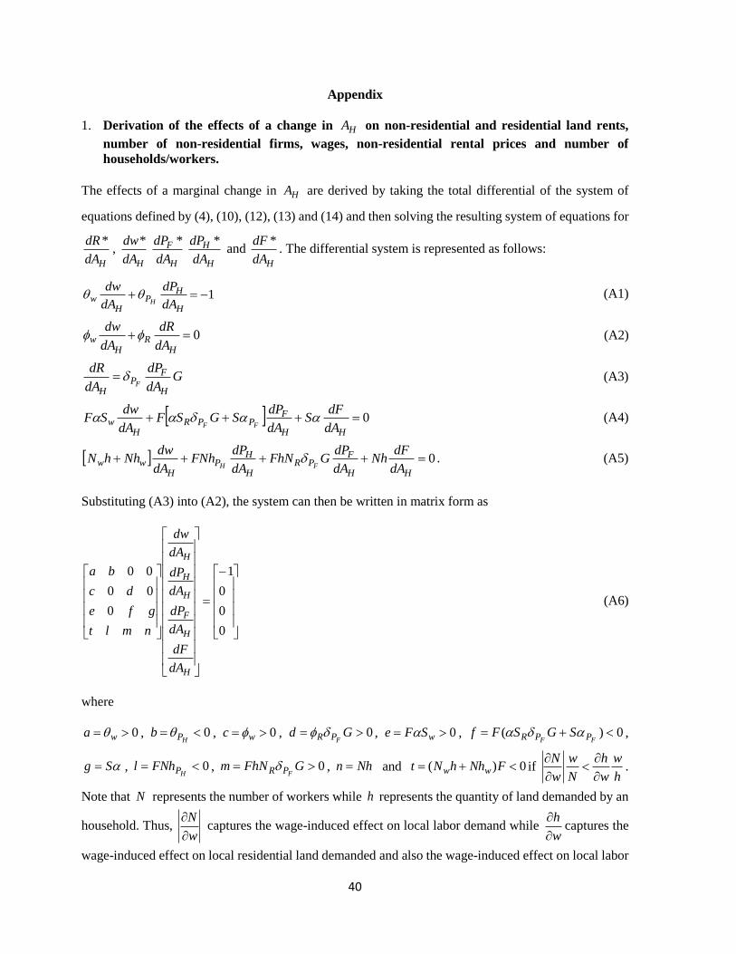
40

Appendix

1. Derivation of the effects of a change in HA on non-residential and residential land rents,

number of non-residential firms, wages, non-residential rental prices and number of

households/workers.

The effects of a marginal change in HA are derived by taking the total differential of the system of

equations defined by (4), (10), (12), (13) and (14) and then solving the resulting system of equations for

HdA

dR *,

HdA

dw*

H

F

dA

dP *

H

H

dA

dP * and

HdA

dF *. The differential system is represented as follows:

1H

HP

Hw

dA

dP

dA

dwH

(A1)

0H

RH

wdA

dR

dA

dw (A2)

GdA

dP

dA

dR

H

FP

HF

(A3)

0HH

FPPR

Hw

dA

dFS

dA

dPSGSF

dA

dwSF

FF (A4)

0HH

FPR

H

HP

Hww

dA

dFNh

dA

dPGFhN

dA

dPFNh

dA

dwNhhN

FH . (A5)

Substituting (A3) into (A2), the system can then be written in matrix form as

0

0

0

1

0

00

00

H

H

F

H

H

H

dA

dF

dA

dP

dA

dP

dA

dw

nmlt

gfe

dc

ba

(A6)

where

0 wa , 0HPb , 0 wc , 0 Gd

FPR , 0 wSFe , 0)( FF PPR SGSFf ,

Sg , 0HPFNhl , 0 GFhNm

FPR , Nhn and 0)( FNhhNt ww if h

w

w

h

N

w

w

N

.

Note that N represents the number of workers while h represents the quantity of land demanded by an

household. Thus, w

N

captures the wage-induced effect on local labor demand while

w

h

captures the

wage-induced effect on local residential land demanded and also the wage-induced effect on local labor

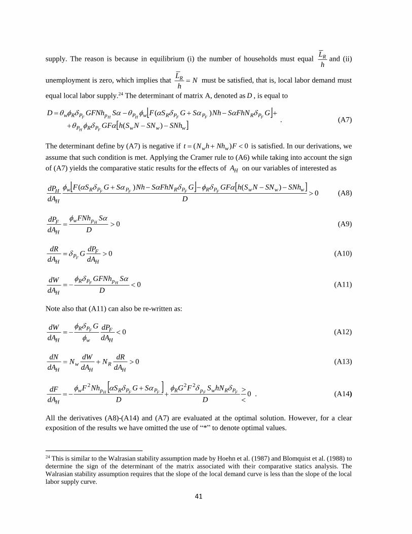
41

supply. The reason is because in equilibrium (i) the number of households must equal h

LR and (ii)

unemployment is zero, which implies that Nh

LR must be satisfied, that is, local labor demand must

equal local labor supply.24 The determinant of matrix A, denoted as D , is equal to

wwwPRP

PRPPRwPpPRw

SNhSNNShGF

GFhNSNhSGSFSGFNhD

FH

FFFHHF

)(

)(

. (A7)

The determinant define by (A7) is negative if 0)( FNhhNt ww is satisfied. In our derivations, we

assume that such condition is met. Applying the Cramer rule to (A6) while taking into account the sign

of (A7) yields the comparative static results for the effects of HA on our variables of interested as

0

)()(

D

SNhSNNShGFGFhNSNhSGSF

dA

dP wwwPRPRPPRw

H

H FFFF

(A8)

0D

SFNh

dA

dPHpw

H

F

(A9)

0H

FP

H dA

dPG

dA

dRF

(A10)

0D

SGFNh

dA

dWHF pPR

H

(A11)

Note also that (A11) can also be re-written as:

0H

F

w

PR

H dA

dPG

dA

dWF

(A12)

0H

RH

wH dA

dRN

dA

dWN

dA

dN (A13)

0

222

D

hNSFG

D

SGSNhF

dA

dFFFFFH PRwpRPPRpw

H

. (A14)

All the derivatives (A8)-(A14) and (A7) are evaluated at the optimal solution. However, for a clear

exposition of the results we have omitted the use of “*” to denote optimal values.

24 This is similar to the Walrasian stability assumption made by Hoehn et al. (1987) and Blomquist et al. (1988) to

determine the sign of the determinant of the matrix associated with their comparative statics analysis. The

Walrasian stability assumption requires that the slope of the local demand curve is less than the slope of the local

labor supply curve.

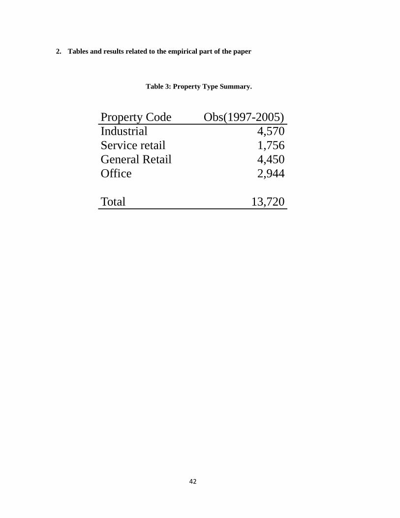
42

2. Tables and results related to the empirical part of the paper

Table 3: Property Type Summary.

Property Code Obs(1997-2005)

Industrial 4,570

Service retail 1,756

General Retail 4,450

Office 2,944

Total 13,720

43

Table 4: Variable Definitions

Variable name Definition

Dependent Variable

lprice Log of sale price

Amenities

Wild Within one mile of national forest, natural area, wilderness area, wildlife area.

regparks20 Within .2 miles of city or county park.

Golf20 Within .2 miles of Golf Course.

Ozone1_90 90th percentile of location's one hour maximum ozone concentration.

d_sea Distance to the sea (miles.)

Crime2000 Crime Level relative to nation average in 2000 CAP Index.

dist_FH Distance to a freeway (miles).

dist_lax Distance to LAX (miles.)

dist_aer Minimum distance to another airport that is not LAX (miles.)

weathf1 Weather Principal Component one (max temperature)

weathf2 Weather Principal Component two.(Cooling Degree Days)

busdistrict1 Principal Component one of distance to Downtwon/Westside Business Districts

busdistrict2 Principal Component two of distance to Downtwon/Westside Business Districts

pasa_chall Distance to Pasadena City hall (miles.)

lbeach_chall Distance to Long Beach City hall (miles.)

rail Indicator that property has rail access.

Neighborhood Characteristics

dens Total non-residential building floor area per square foot land area - one-third mile

radius.

DQprice Median house value in zip code and year of sale.

Bachorhgh Number of residents in commute distance with college degree

Empl2 Employment in retail clothing and acessories for establishments in the zip code.

Empl5 Employment ineating and drinking establishments in the zip code.

lpksup Logged estimated density of parking in 1/3 mile radius (own excluded).

llandval Logged assesor estimated land value in 1/3 mile radius (own excluded). (millions)

Property Characteristics

pcsqft Property area (square feet)

park Parking area (square feet)

bldg Building floor area (square feet)

age Age of main building on property

cnloc Corner location

Construction indicators Categories are: concrete (base), brick, frame, mixed, other, missing

Condition indicators Condition categories: A (base),E,F,G,P, missing.

Property categories indicators for industrial (base), three retail types and office, for pooled

specification only

Zoning Zoning designation of property.

Year dummies Indicators for each year of sale (year1997-year2005)

ltind Indicator for light industrial (industrial property specification only)

looff Low rise office indicator (office properties specification only)

offres Office-residential dual use indicator (office properties specification only)

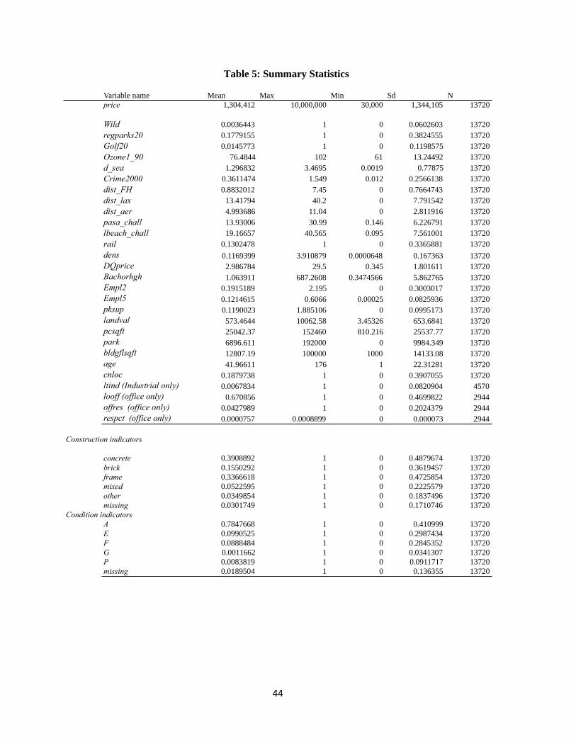
44

Table 5: Summary Statistics

Variable name Mean Max Min Sd N

price 1,304,412 10,000,000 30,000 1,344,105 13720

Wild 0.0036443 1 0 0.0602603 13720

regparks20 0.1779155 1 0 0.3824555 13720

Golf20 0.0145773 1 0 0.1198575 13720

Ozone1_90 76.4844 102 61 13.24492 13720

d_sea 1.296832 3.4695 0.0019 0.77875 13720

Crime2000 0.3611474 1.549 0.012 0.2566138 13720

dist_FH 0.8832012 7.45 0 0.7664743 13720

dist_lax 13.41794 40.2 0 7.791542 13720

dist_aer 4.993686 11.04 0 2.811916 13720

pasa_chall 13.93006 30.99 0.146 6.226791 13720

lbeach_chall 19.16657 40.565 0.095 7.561001 13720

rail 0.1302478 1 0 0.3365881 13720

dens 0.1169399 3.910879 0.0000648 0.167363 13720

DQprice 2.986784 29.5 0.345 1.801611 13720

Bachorhgh 1.063911 687.2608 0.3474566 5.862765 13720

Empl2 0.1915189 2.195 0 0.3003017 13720

Empl5 0.1214615 0.6066 0.00025 0.0825936 13720

pksup 0.1190023 1.885106 0 0.0995173 13720

landval 573.4644 10062.58 3.45326 653.6841 13720

pcsqft 25042.37 152460 810.216 25537.77 13720

park 6896.611 192000 0 9984.349 13720

bldgflsqft 12807.19 100000 1000 14133.08 13720

age 41.96611 176 1 22.31281 13720

cnloc 0.1879738 1 0 0.3907055 13720

ltind (Industrial only) 0.0067834 1 0 0.0820904 4570

looff (office only) 0.670856 1 0 0.4699822 2944

offres (office only) 0.0427989 1 0 0.2024379 2944

respct (office only) 0.0000757 0.0008899 0 0.000073 2944

Construction indicators

concrete 0.3908892 1 0 0.4879674 13720

brick 0.1550292 1 0 0.3619457 13720

frame 0.3366618 1 0 0.4725854 13720

mixed 0.0522595 1 0 0.2225579 13720

other 0.0349854 1 0 0.1837496 13720

missing 0.0301749 1 0 0.1710746 13720

Condition indicators

A 0.7847668 1 0 0.410999 13720

E 0.0990525 1 0 0.2987434 13720

F 0.0888484 1 0 0.2845352 13720

G 0.0011662 1 0 0.0341307 13720

P 0.0083819 1 0 0.0911717 13720

missing 0.0189504 1 0 0.136355 13720

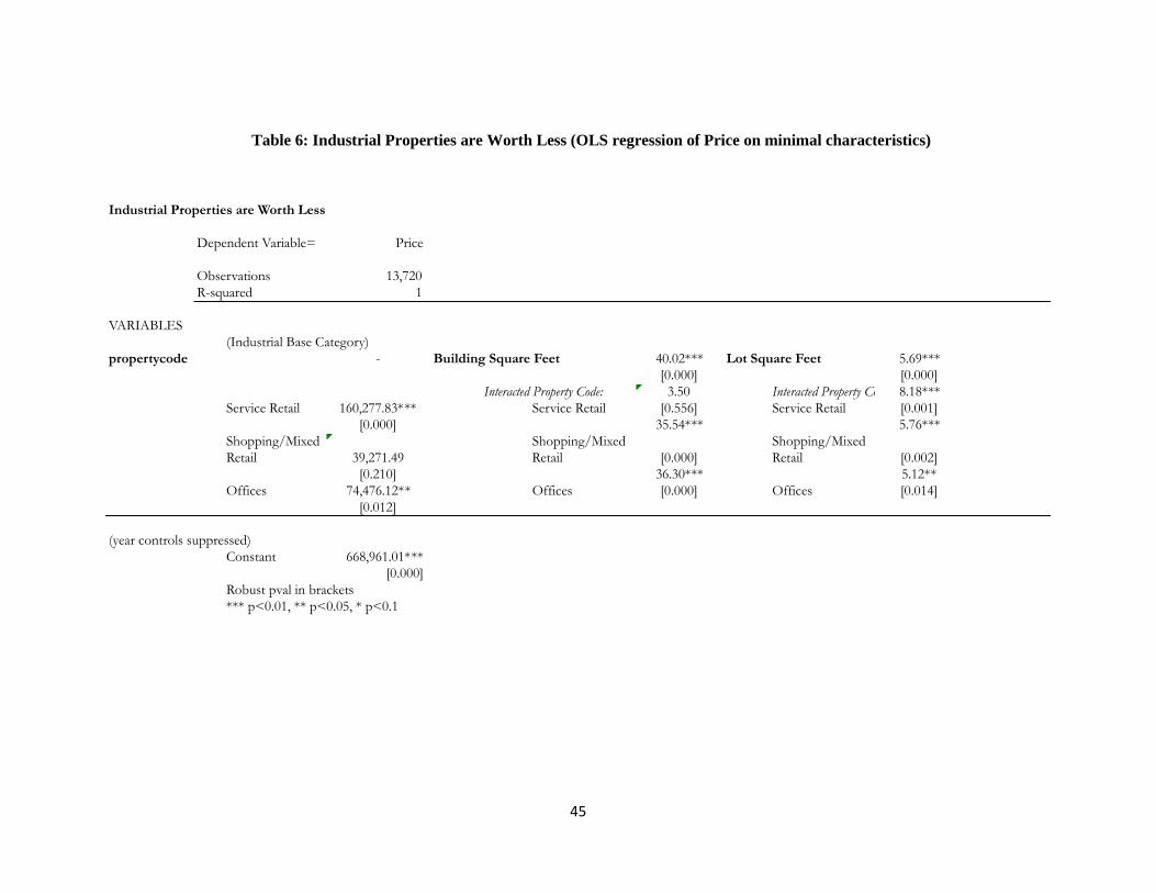
45

Table 6: Industrial Properties are Worth Less (OLS regression of Price on minimal characteristics)

Industrial Properties are Worth Less

Dependent Variable= Price

Observations 13,720

R-squared 1

VARIABLES

(Industrial Base Category)

propertycode - Building Square Feet 40.02*** Lot Square Feet 5.69***

[0.000] [0.000]

Interacted Property Code: 3.50 Interacted Property Code: 8.18***

Service Retail 160,277.83*** Service Retail [0.556] Service Retail [0.001]

[0.000] 35.54*** 5.76***

Shopping/Mixed

Retail 39,271.49

Shopping/Mixed

Retail [0.000]

Shopping/Mixed

Retail [0.002]

[0.210] 36.30*** 5.12**

Offices 74,476.12** Offices [0.000] Offices [0.014]

[0.012]

(year controls suppressed)

Constant 668,961.01***

[0.000]

Robust pval in brackets

*** p<0.01, ** p<0.05, * p<0.1

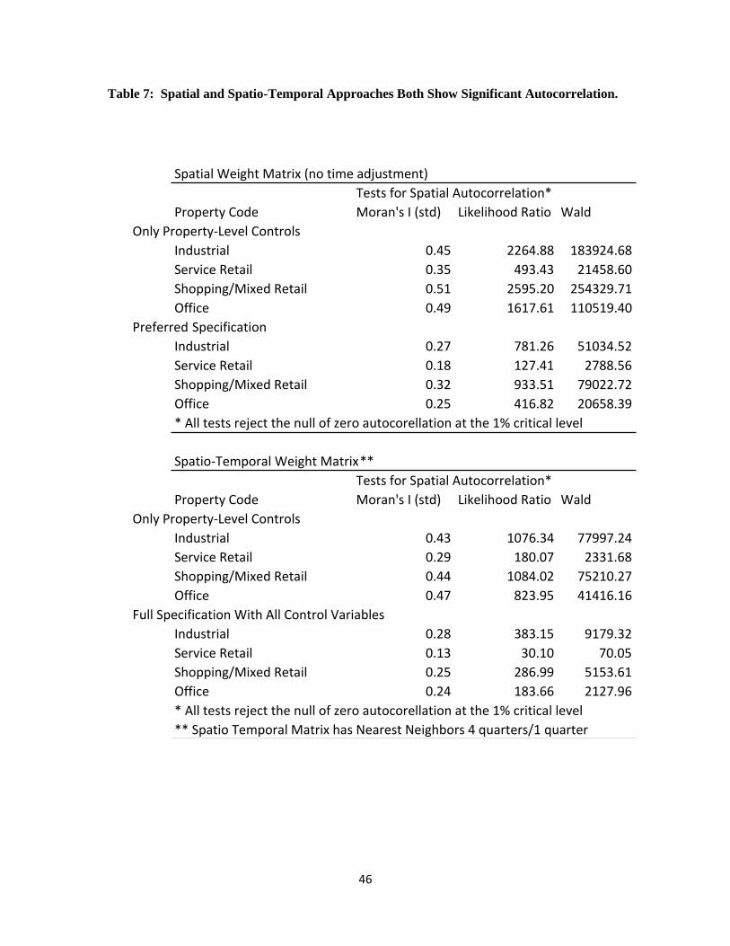
46

Table 7: Spatial and Spatio-Temporal Approaches Both Show Significant Autocorrelation.

SpatialWeightMatrix(notimeadjustment)

TestsforSpatialAutocorrelation*

PropertyCode Moran'sI(std) LikelihoodRatio Wald

OnlyProperty-LevelControls

Industrial 0.45 2264.88 183924.68

ServiceRetail 0.35 493.43 21458.60

Shopping/MixedRetail 0.51 2595.20 254329.71

Office 0.49 1617.61 110519.40

PreferredSpecification

Industrial 0.27 781.26 51034.52

ServiceRetail 0.18 127.41 2788.56

Shopping/MixedRetail 0.32 933.51 79022.72

Office 0.25 416.82 20658.39

*Alltestsrejectthenullofzeroautocorellationatthe1%criticallevel

Spatio-TemporalWeightMatrix**

TestsforSpatialAutocorrelation*

PropertyCode Moran'sI(std) LikelihoodRatio Wald

OnlyProperty-LevelControls

Industrial 0.43 1076.34 77997.24

ServiceRetail 0.29 180.07 2331.68

Shopping/MixedRetail 0.44 1084.02 75210.27

Office 0.47 823.95 41416.16

FullSpecificationWithAllControlVariables

Industrial 0.28 383.15 9179.32

ServiceRetail 0.13 30.10 70.05

Shopping/MixedRetail 0.25 286.99 5153.61

Office 0.24 183.66 2127.96

*Alltestsrejectthenullofzeroautocorellationatthe1%criticallevel

**SpatioTemporalMatrixhasNearestNeighbors4quarters/1quarter

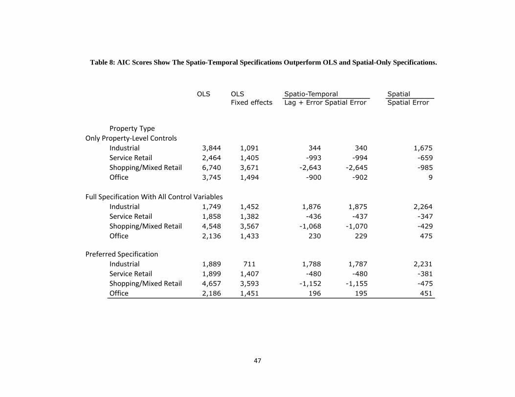
47

Table 8: AIC Scores Show The Spatio-Temporal Specifications Outperform OLS and Spatial-Only Specifications.

OLS OLS Spatio-Temporal Spatial

Fixed effects Lag + Error Spatial Error Spatial Error

PropertyTypeOnlyProperty-LevelControls

Industrial 3,844 1,091 344 340 1,675

ServiceRetail 2,464 1,405 -993 -994 -659

Shopping/MixedRetail 6,740 3,671 -2,643 -2,645 -985

Office 3,745 1,494 -900 -902 9

FullSpecificationWithAllControlVariablesIndustrial 1,749 1,452 1,876 1,875 2,264

ServiceRetail 1,858 1,382 -436 -437 -347

Shopping/MixedRetail 4,548 3,567 -1,068 -1,070 -429

Office 2,136 1,433 230 229 475

PreferredSpecificationIndustrial 1,889 711 1,788 1,787 2,231

ServiceRetail 1,899 1,407 -480 -480 -381

Shopping/MixedRetail 4,657 3,593 -1,152 -1,155 -475

Office 2,186 1,451 196 195 451

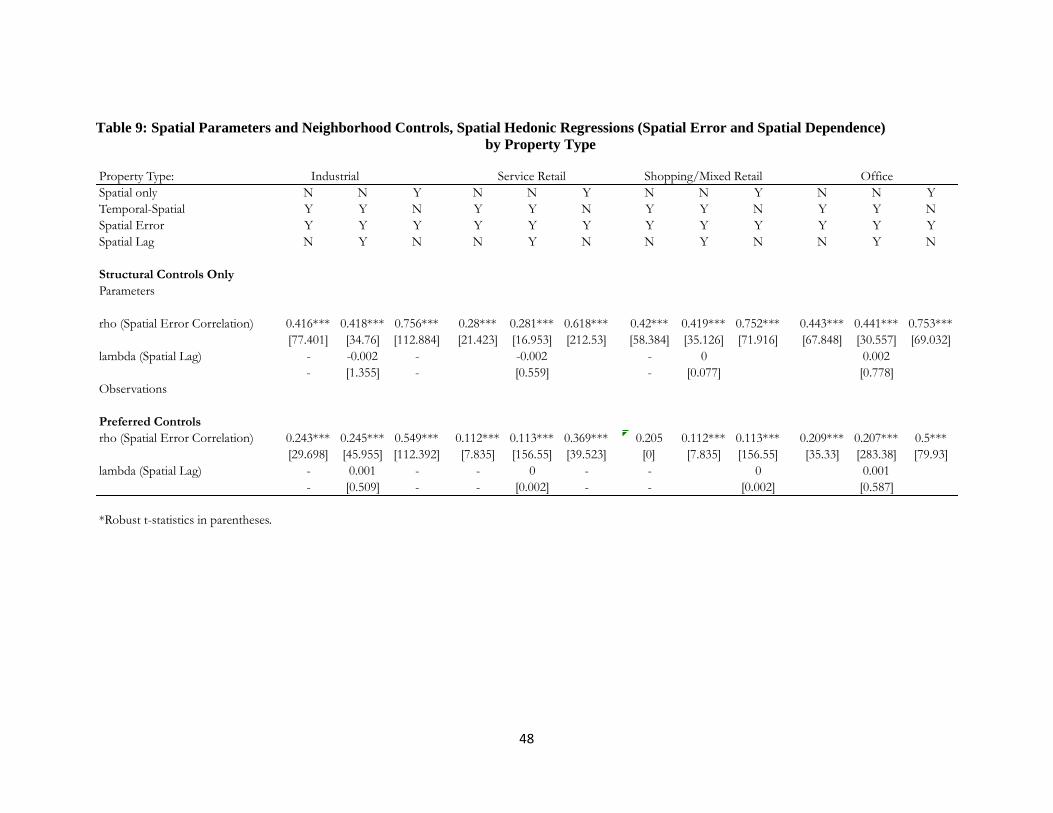
48

Table 9: Spatial Parameters and Neighborhood Controls, Spatial Hedonic Regressions (Spatial Error and Spatial Dependence)

by Property Type

Property Type: Industrial Service Retail Office

Spatial only N N Y N N Y N N Y N N Y

Temporal-Spatial Y Y N Y Y N Y Y N Y Y N

Spatial Error Y Y Y Y Y Y Y Y Y Y Y Y

Spatial Lag N Y N N Y N N Y N N Y N

Structural Controls Only

Parameters

rho (Spatial Error Correlation) 0.416*** 0.418*** 0.756*** 0.28*** 0.281*** 0.618*** 0.42*** 0.419*** 0.752*** 0.443*** 0.441*** 0.753***

[77.401] [34.76] [112.884] [21.423] [16.953] [212.53] [58.384] [35.126] [71.916] [67.848] [30.557] [69.032]

lambda (Spatial Lag) - -0.002 - -0.002 - 0 0.002

- [1.355] - [0.559] - [0.077] [0.778]

Observations

Preferred Controls

rho (Spatial Error Correlation) 0.243*** 0.245*** 0.549*** 0.112*** 0.113*** 0.369*** 0.205 0.112*** 0.113*** 0.209*** 0.207*** 0.5***

[29.698] [45.955] [112.392] [7.835] [156.55] [39.523] [0] [7.835] [156.55] [35.33] [283.38] [79.93]

lambda (Spatial Lag) - 0.001 - - 0 - - 0 0.001

- [0.509] - - [0.002] - - [0.002] [0.587]

*Robust t-statistics in parentheses.

Shopping/Mixed Retail

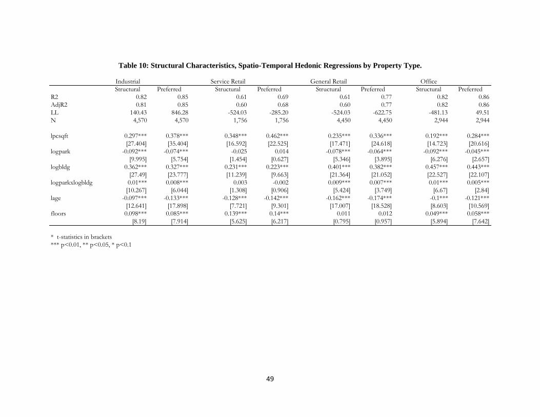
49

Table 10: Structural Characteristics, Spatio-Temporal Hedonic Regressions by Property Type.

Industrial Service Retail General Retail Office

Structural Preferred Structural Preferred Structural Preferred Structural Preferred

R2 0.82 0.85 0.61 0.69 0.61 0.77 0.82 0.86

AdjR2 0.81 0.85 0.60 0.68 0.60 0.77 0.82 0.86

LL 140.43 846.28 -524.03 -285.20 -524.03 -622.75 -481.13 49.51

N 4,570 4,570 1,756 1,756 4,450 4,450 2,944 2,944

lpcsqft 0.297*** 0.378*** 0.348*** 0.462*** 0.235*** 0.336*** 0.192*** 0.284***

[27.404] [35.404] [16.592] [22.525] [17.471] [24.618] [14.723] [20.616]

logpark -0.092*** -0.074*** -0.025 0.014 -0.078*** -0.064*** -0.092*** -0.045***

[9.995] [5.754] [1.454] [0.627] [5.346] [3.895] [6.276] [2.657]

logbldg 0.362*** 0.327*** 0.231*** 0.223*** 0.401*** 0.382*** 0.457*** 0.443***

[27.49] [23.777] [11.239] [9.663] [21.364] [21.052] [22.527] [22.107]

logparkxlogbldg 0.01*** 0.008*** 0.003 -0.002 0.009*** 0.007*** 0.01*** 0.005***

[10.267] [6.044] [1.308] [0.906] [5.424] [3.749] [6.67] [2.84]

lage -0.097*** -0.133*** -0.128*** -0.142*** -0.162*** -0.174*** -0.1*** -0.121***

[12.641] [17.898] [7.721] [9.301] [17.007] [18.528] [8.603] [10.569]

floors 0.098*** 0.085*** 0.139*** 0.14*** 0.011 0.012 0.049*** 0.058***

[8.19] [7.914] [5.625] [6.217] [0.795] [0.957] [5.894] [7.642]

* t-statistics in brackets

*** p<0.01, ** p<0.05, * p<0.1

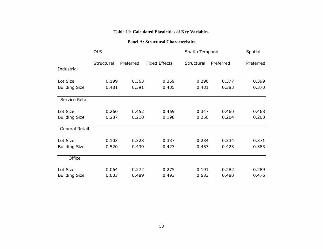
50

Table 11: Calculated Elasticities of Key Variables.

Panel A: Structural Characteristics

OLS Spatio-Temporal Spatial

Structural Preferred Fixed Effects Structural Preferred Preferred

Industrial

Lot Size 0.199 0.363 0.359 0.296 0.377 0.399

Building Size 0.481 0.391 0.405 0.431 0.383 0.370

Service Retail

Lot Size 0.260 0.452 0.469 0.347 0.460 0.468

Building Size 0.287 0.210 0.198 0.250 0.204 0.200

General Retail

Lot Size 0.103 0.323 0.337 0.234 0.334 0.371

Building Size 0.520 0.439 0.423 0.453 0.423 0.383

Office

Lot Size 0.064 0.272 0.275 0.191 0.282 0.289

Building Size 0.603 0.489 0.493 0.533 0.480 0.476

51

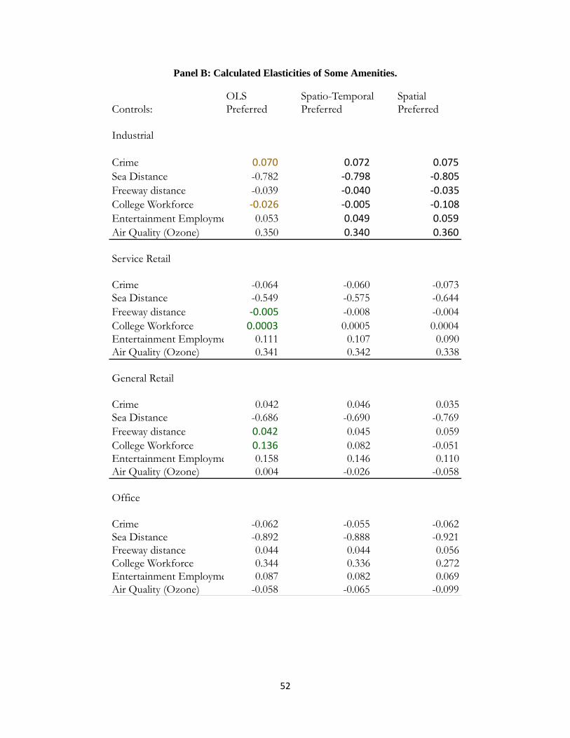
52

Panel B: Calculated Elasticities of Some Amenities.

OLS Spatio-Temporal Spatial

Controls: Preferred Preferred Preferred

Industrial

Crime 0.070 0.072 0.075Sea Distance -0.782 -0.798 -0.805

Freeway distance -0.039 -0.040 -0.035

College Workforce -0.026 -0.005 -0.108

Entertainment Employment 0.053 0.049 0.059

Air Quality (Ozone) 0.350 0.340 0.360

Service Retail

Crime -0.064 -0.060 -0.073

Sea Distance -0.549 -0.575 -0.644

Freeway distance -0.005 -0.008 -0.004

College Workforce 0.0003 0.0005 0.0004

Entertainment Employment 0.111 0.107 0.090

Air Quality (Ozone) 0.341 0.342 0.338

General Retail

Crime 0.042 0.046 0.035

Sea Distance -0.686 -0.690 -0.769

Freeway distance 0.042 0.045 0.059

College Workforce 0.136 0.082 -0.051

Entertainment Employment 0.158 0.146 0.110

Air Quality (Ozone) 0.004 -0.026 -0.058

Office

Crime -0.062 -0.055 -0.062

Sea Distance -0.892 -0.888 -0.921

Freeway distance 0.044 0.044 0.056

College Workforce 0.344 0.336 0.272

Entertainment Employment 0.087 0.082 0.069

Air Quality (Ozone) -0.058 -0.065 -0.099

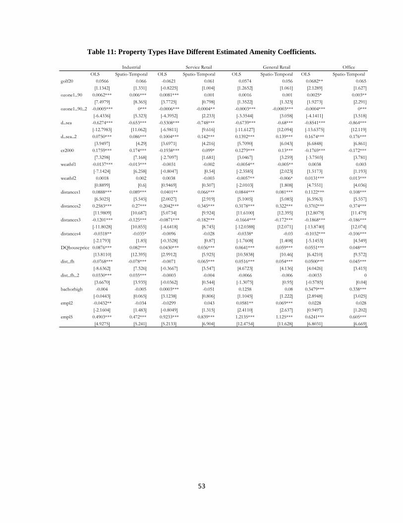
53

Table 11: Property Types Have Different Estimated Amenity Coefficients.

Industrial Service Retail General Retail Office

OLS Spatio-Temporal OLS Spatio-Temporal OLS Spatio-Temporal OLS Spatio-Temporal

golf20 0.0566 0.066 -0.0621 0.061 0.0574 0.056 0.0682** 0.065

[1.1342] [1.331] [-0.8225] [1.004] [1.2652] [1.061] [2.1289] [1.627]

ozone1_90 0.0062*** 0.006*** 0.0081*** 0.001 0.0016 0.001 0.0025* 0.003**

[7.4979] [8.365] [3.7725] [0.798] [1.3522] [1.323] [1.9273] [2.291]

ozone1_90_2 -0.0005*** 0*** -0.0006*** -0.0004** -0.0003*** -0.0003*** -0.0004*** 0***

[-6.4336] [5.323] [-4.3952] [2.233] [-3.3544] [3.058] [-4.1411] [3.518]

d_sea -0.6274*** -0.653*** -0.5308*** -0.748*** -0.6739*** -0.68*** -0.8541*** -0.864***

[-12.7983] [11.062] [-6.9811] [9.616] [-11.6127] [12.094] [-13.6375] [12.119]

d_sea_2 0.0750*** 0.086*** 0.1004*** 0.142*** 0.1392*** 0.139*** 0.1674*** 0.176***

[3.9497] [4.29] [3.6971] [4.216] [5.7090] [6.043] [6.6848] [6.861]

cr2000 0.1759*** 0.174*** -0.1938*** 0.099* 0.1279*** 0.13*** -0.1769*** -0.172***

[7.3298] [7.168] [-2.7097] [1.681] [3.0467] [3.259] [-3.7503] [3.781]

weathf1 -0.0137*** -0.013*** -0.0031 -0.002 -0.0054** -0.005** 0.0038 0.003

[-7.1424] [6.258] [-0.8047] [0.54] [-2.3585] [2.023] [1.5173] [1.193]

weathf2 0.0018 0.002 0.0038 -0.003 -0.0057** -0.006* 0.0131*** 0.013***

[0.8899] [0.6] [0.9469] [0.507] [-2.0103] [1.808] [4.7551] [4.036]

distances1 0.0888*** 0.089*** 0.0401** 0.066*** 0.0844*** 0.081*** 0.1122*** 0.108***

[6.5025] [5.545] [2.0027] [2.919] [5.1005] [5.085] [6.5963] [5.557]

distances2 0.2583*** 0.27*** 0.2042*** 0.345*** 0.3178*** 0.322*** 0.3702*** 0.374***

[11.9809] [10.687] [5.0734] [9.924] [11.6100] [12.395] [12.8079] [11.479]

distances3 -0.1201*** -0.125*** -0.0871*** -0.182*** -0.1664*** -0.172*** -0.1868*** -0.186***

[-11.8028] [10.855] [-4.6418] [8.745] [-12.0388] [12.071] [-13.8740] [12.074]

distances4 -0.0318** -0.035* -0.0096 -0.028 -0.0338* -0.03 -0.1032*** -0.106***

[-2.1793] [1.85] [-0.3528] [0.87] [-1.7608] [1.408] [-5.1453] [4.549]

DQhouseprice 0.0876*** 0.082*** 0.0430*** 0.036*** 0.0641*** 0.059*** 0.0551*** 0.048***

[13.8110] [12.395] [2.9912] [5.925] [10.5838] [10.46] [6.4210] [9.572]

dist_fh -0.0768*** -0.078*** -0.0071 0.065*** 0.0516*** 0.054*** 0.0500*** 0.045***

[-8.6362] [7.526] [-0.3667] [3.547] [4.6723] [4.136] [4.0426] [3.415]

dist_fh_2 0.0330*** 0.035*** -0.0003 -0.004 -0.0066 -0.006 -0.0033 0

[3.6670] [3.935] [-0.0362] [0.544] [-1.3075] [0.95] [-0.5785] [0.04]

bachorhigh -0.004 -0.005 0.0003*** -0.051 0.1258 0.08 0.3479*** 0.338***

[-0.0443] [0.065] [3.1238] [0.806] [1.1045] [1.222] [2.8948] [3.025]

empl2 -0.0432** -0.034 -0.0299 0.043 0.0581** 0.069*** 0.0228 0.028

[-2.1604] [1.483] [-0.8049] [1.315] [2.4110] [2.637] [0.9497] [1.202]

empl5 0.4903*** 0.472*** 0.9233*** 0.839*** 1.2135*** 1.125*** 0.6241*** 0.605***

[4.9275] [5.241] [5.2133] [6.904] [12.4754] [11.628] [6.8031] [6.669]

54

Nova School of Business and Economics

Faculdade de Economia

Universidade Nova de Lisboa

Campus de Campolide

1099-032 Lisboa PORTUGAL

Tel.: +351 213 801 600

www.novasbe.pt