Working Paper 95-46 Departamento de Economía de la Empresa

Business Economics Series 06 Universidad Carlos III de Madrid

October 1995 Calle Madrid, 126

28903 Getafe (Spain)

Fax (34-1) 624-9875

EMPIRICAL EVIDENCE ON THE IMPACT�

OF EUROPEAN INSIDER TRADING REGULATIONS�

Javier Estrada and J. Ignacio Peña •�

Abstract _�

We evaluate in this artic1e the impact of the regulations on insider trading introduced between�

1988 and 1994 on ten European securities markets. We consider the temporal behavior and the�

distributions of abnormal returns, market models, and time series models of time-varying mean�

returns and volatility, and conc1ude that the bulk of the evidence suggests that these regulations�

have had little (if any) impact on the series of returns of the markets in our sample.�

Key Words�

Insider trading. Securities Regulation. EU Directives.�

• Departamento de Economía de la Empresa, Universidad Carlos III de Madrid. EMAILS:

<estrada@eco.uc3m.es>, < ypenya@eco.uc3m.es>. Correspondingauthor: Javier Estrada. We

would like to thank Rich Kihlstrom, Clas Wihlborg, participants of seminars at Gothenburg

University (Gothenburg, Sweden) and Torcuato Di Tella University (Buenos Aires, Argentina),

and participants of the 12th Annual Meeting of the European Association of Law and Economics

(Gerzensee, Switzerland) for helpful cornments and suggestions. We are also indebted to Eirik

Bunaes, Corrado Conti, Michael Kremsner, C. Lempereur, Frédéric Perier, and Georg Wittich

for helpful information regarding European insider trading regulations. Finally, we are indebted

to Eudald Canadell for providing helpful contacts. The views expressed below and any errors that

may remain are entirely our own.

--- _..__._---~---~-------,-:-----------------------------

2

1- INTRODUCTION

The academic discussion on the issue of insider trading and its regulation started in the

mid-1960s with the pathbreaking book by Manne (1966). Since then, a massive literature

produced by lawyers, economists, and financial economists has addressed the theoretieal impact

of insider trading regulation (ITR) on securities markets. 1 This article is an attempt to evaluate

the impact of ITR on securities markets from an empirieal point of view.

The empiriealliterature on insider trading has basieally followed three approaches. The

first approach consists of determining, using data self reported by insiders, whether insiders

obtain abnormal retums;2 see, for example, the seminal articles by Jaffe (1974) and Finnerty

(1976). The general consensus of this literature seems to be that insiders do obtain abnormal

retums. To illustrate, Seyhun (1992) concludes that insiders obtained annual abnormal retums

of 3.5% before 1980, 5.1 % between 1980 and 1984, and 7% after 1984. This trend in insiders'

abnormal retums is obviously at odds with the tightening of ITR observed in the US during the

1980s. Thus, Seyhun (1992) concludes that the increase in statutory sanctions during that period

did not have a detrimental impact on insiders' abnormal profits.

The second approach seeks to infer the presence of insiders from time series of stock

retums. This approach basieally consists of analyzing the behavior of stocks around sorne

corporate announcement in order to determine abnormal pattems that may hint the presence of

insiders; see, for example, Keown and Pinkerton (1981) analyzing merger announcements, and

JoOO and Lang (1991) analyzing dividend announcements. The consensus of this literature seems

to be that stock prices do move significantly before corporate announcements, and that they do

it in a direction consistent with the presence of insiders in the market.3 To illustrate, Keown and

Pinkerton (1981) find that cumulative average abnormal retums become positive 25 days prior

1 Macey (1991) and Estrada (1994) may be useful (non-tecOOical) introductions to the topie.

2 Under Section 16 of the Securities Exchange Act of 1934, directors, officers and majority stockholders (owners of more than 10% of equity) must report their securities holdings and changes in holdings to the SEC on a monthly basis.

3 See, however, Jarrell and Poulsen (1989), who argue that the abnormal behavior of stock prices before corporate announcements can be largely explained by rumors in the news media.

" """"-"--------------------,-------------------------­

3

to the merger announcement date, that approximately half of their increase occurs prior to that

day, and that a significant increase in trading volume precedes the announcement date. 4

Finally, a third and more novel approach consists of using information that makes it

possible to identify exactly when insiders enter the market and what transactions they make, thus

making it feasible to analyze the impact of insider trading on the stocks involved. Meulbroek

(1992), using SEC nonpublic files, studies the transactions of 320 individuals charged with

insider trading by the SEC; Comell and Sirri (1992), on the other hand, use court records to

analyze the impact of insiders' transactions around the Anheuser-Busch's 1982 tender offer for

Campbell-Taggart. To illustrate, Meulbroek (1992) finds that, in the days in which insiders made

transactions, the mean abnormal retum is 3.06% (and statistical1y significant), the cumulative

abnormal retum is 6.85 % (and also statistical1y significant), and that in 81 % of those days stock

prices move in the same direction as they do upon public announcement of the relevant events.5

Our purpose is neither to determine whether European insiders have obtained abnormal

retums, nor to determine whether European insiders traded before corporate announcements, nor

to evaluate the impact of the transactions of European insiders on selected stocks. Rather, our

goal is to evaluate the impact of ITR on the behavior of European securities markets. More

precisely, we attempt to evaluate the impact of the regulations on insider trading imposed in ten

European securities markets between 1988 and 1994. To that purpose, we surnmarize the

behavior of each market in an index of representative stocks and ask two questions: First, we

ask what changes are observed in several characteristics of the series of retums of each market

after the imposition or tightening of ITR; and, second, we ask whether such changes, if any,

have cornmon features across the ten markets. Thus, if after controlling for factors affecting aH

markets, we observe that the markets in which ITR was imposed or tightened exhibit the same

4 Keown and Pinkerton (1981) also find that the increase in trading volume does not correspond to an increase in the trading volume of registered insiders, and infer that most insider trading is carried out through third parties in order to avoid detection.

5 This last result gives support to the argument that insider trading increases the informational efficiency of securities markets by correcting securities prices in the right direction. Such a result, informal1y suggested by Manne (1966), has been formal1y established by Leland (1994) and Estrada (1995), among others.

..-...---------------------r---------­

4

qualitative changes, then we will conclude that those changes are likely to stem from the

regulatory event. If, on the other hand, we observe no common pattern of change across

markets, then we will conclude that the observed changes, if any, are likely to be due to factors

missing from the model rather than to the imposition or tightening of ITR.

Our study is different from previous empirical studies on insider trading in several

aspects. First, most previous studies have been performed for US markets; our study considers

European markets. Second, most previous event studies on insider trading use corporate

announcements as the events to be analyzed; the events considered in our study are the

imposition or tightening of ITR. Third, most previous studies use data self-reported by insiders

or data on individual stocks; our study uses aggregate data that summarizes in an index the

behavior of each market. Fourth, as mentioned aboye, most previous studies focus on

determining whether insiders obtain abnormal returns, or on detecting the presence of insiders

before corporate announcements, or on evaluating the impact of insider trading on selected

stocks; our study seeks to evaluate the impact of ITR on several characteristics of the series of

returns of ten European securities markets.

The rest of this article is organized as follows. In part 11, we describe the data and the

basic methodology. In part 111, we assess the impact of ITR on the temporal behavior and the

distributions of abnormal returns, and on the market models that generate these returns. In part

IV, we estimate GARCH models in order to evaluate the impact of ITR on mean returns and

volatility. And, finally, in part V, we summarize the most important conclusions of the analysis.

An appendix at the end of the article contains some tables and pictures, and a brief account of

the evolution of ITR in the ten markets in our sample.

11- DATA AND METHODOLOGY

The sample under consideration consists of ten European markets that have either

introduced or tightened ITR between 1988 and 1994; these markets are Austria (AUS), Belgium

(BEL), Denmark (DEN), France (FRA), Germany (GER), Holland (HOL), Italy (ITA), Norway

(NOR), Sweden (SWE) , and Switzerland (SWI). The behavior of each of these markets is

summarized by the Financial Times Actuaries World Index, published daily in the Financial

Times. The sample size varies for each market; whenever possible, daily data has been gathered

beginning approximately ayear and a half before the imposition or tightening of ITR, and ayear

--------_._---------------,----------------------- ,---­

5

and a half after that regulatory evento The largest sample size is that of France (1,326

observations) and the smallest that of Germany (301 observations).

The regulatory events considered in this study are either the imposition or tightening of

ITR. The former applies to those markets that prohibited ITR for the first time (Italy); the latter,

on the other hand, applies to those markets that had ITR but tightened it in the sense that insider

trading became a criminal offense (Austria), that penalties were increased (Sweden), or that the

scope of the offense was broadened (Norway). One regulatory event is considered in seven out

of the ten markets analyzed, and two regulatory events are considered in the other three markets;

that yields a total of thirteen regulatory events, the earliest of which occurred in July of 1988

(in Switzerland), and the latest in August of 1994 (in Germany). Section A8 of the appendix

contains a very brief account of the regulatory process in each of the markets in our sample.6

Table 1 below surnmarizes only the dates of the regulatory events considered, the sample period

for each market, and the number of observations in each sample and subsample.

TABLE 1: Event Dates, Sample Periods, and Sample Sizes

Market Event 1 Event 2 Sample Period T TI U T3

AUS Oct-01-1993 Apr-01-1992 I Feb-28-1995 759 391 368 BEL Sep-16-1989 Jan-01-1991 Mar-Ol-1988 I Jun-30-1992 1130 403 336 391 DEN Aug-01-1991 Feb-01-1990 I Jan-29-1993 781 389 392 FRA Jan-24-1988 Jul-21-1990 Jan-01-1987 I Jan-31-1992 1326 276 650 400 GER Aug-01-1994 Jan-01-1994 I Feb-28-1995 301 149 152 HOL Feb-16-1989 Aug-03-1987 I Ago-31-1990 804 402 402 ITA May-21-1991 Nov-01-1989 I Nov-30-1992 803 403 400 NOR Feb-10-1992 Mar-01-1993 Aug-01-1990 I Aug-31-1994 1065 397 275 393 SWE Feb-01-1991 Aug-01-1989 I Jul-31-1992 783 392 391 SWI Ju\-01-1988 Jan-01-1987 I Dec-29-1989 781 390 391

T=number of observations for the whole sample period, TI =number of observations before the first regulatory event, U=number of observations after the first regulatory event (or between events in markets with two events), and T3 =number of observations after the second regulatory evento

In order to isolate the impact of ITR from the impact of other variables affecting aH

European markets, we use the standard methodology for event studies for daily data developed

by Brown and Wamer (1985). Thus, we estimate a market model of the form

6 An extensive review of American, European, and Japanese regulations on insider trading can be found in Gaillard (1992).

______ L-- _

6

(1)

where R¡t is the retum on the ith market, Rmt is the retum on the aggregate European market,

a¡ and {3¡ are coefficients to be estimated, €it is an error term, and the subscripts i and t index

markets and time (trading days), respectively.7 The coefficients a and {3 are estimated by OLS,

and their standard errors are based on the Newey-West heteroskedasticity- and autocorrelation­

consistent covariance matrix. 8 The retum on the aggregate European market is computed as an

equally-weighted average of the retums on twelve European markets.9

The series analyzed for each market is the series of residuals (fiJ, which are given by

(2)

Note that these residuals are excess (or abnormal) retums; therefore, throughout the anicle, we

will refer to them as residuals, excess retums, abnormal retums, or, simply, as retums. In order

to assess the impact of ITR on mean retums and volatility, we will estimate GARCH models in

pan IV. But we address before the impact of ITR on the temporal behavior and the distribution

of abnormal retums, and on the market models that generate these retums. 1O

III- MARKET MODELS AND ABNORMAL RETURNS

We evaluate in this pan the impact of ITR using four different approaches. First, we

evaluate the temporal behavior of abnormal retums in order to assess the aggregate impact of

ITR on the ten markets in the sample. Second, we evaluate whether the introduction or

tightening of ITR has lowered the average cost of capital of the firms in each market, and, more

7 Retums for all markets are defined as the first difference of the naturallogarithm of each index; that is, ~ = 100*[ln(IJ-In(II_I)], where II is the Financial Times Index on day t.

8 There exist other methods to estimate market models; see, for example, Scholes and Williams (1977). However, as shown by Brown and Wamer (1985), these more sophisticated methods do not produce significant improvements over OLS. See also Lo and MacKinlay (1990).

9 These markets are Austria, Belgium, Denrnark, England, France, Germany, Holland, Italy, Norway, Spain, Sweden, and Switzerland.

ID Throughout the anicle all conclusions are drawn at the 5 % significance level.

~~~~--- -----------...,........----------------------- ._--_.�

7

generally, whether the regulatory events caused a change in the models that generate abnormal�

returns. Third, we analyze preliminary evidence on the impact of ITR on mean returns and�

volatility. And, finally, we evaluate the impact of ITR on the pattern of linear and nonlinear�

dependencies in stock returns.�

1.- Abnormal Returns

The aggregate impact of ITR on the ten markets in the sample can be gathered by

analyzing the partern of abnormal returns before and after the imposition or tightening of this

regulation. To that effect, we focus on the first regulatory event in each country, thus analyzing

the impact of ten events. In order to avoid event-driven biases, we first estimate the coefficients

a and {3 using data for the first 200 trading days before the regulatory event. 11 Then, for each

of the 200 trading days around the event (100 days before and 100 days after), we compute the

daily average abnormal return (AAR), which is given by

(3)

where NI is the number of markets with returns available on trading day t. We also compute the

cumulative average abnormal return (CAAR) between any two trading days t] and tú this CAAR

is given by

~ ~ (4)CAAR,¡ = L AAR, .� '='¡�

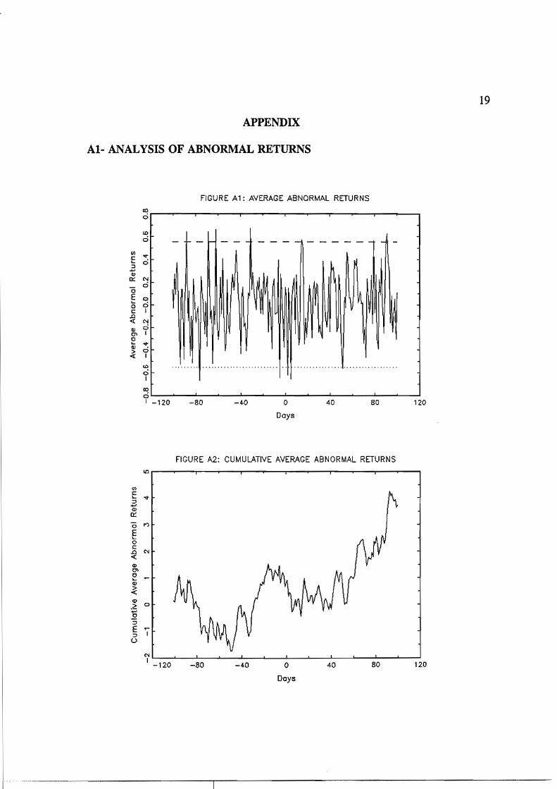
If the aggregate impact of ITR on the ten securities markets in the sample were nil, then

both the AARs and the CAARs would fluctuate randomly over time. Figures Al and A2 in

section Al of the appendix plot the AARs and the CAARs, respectively, for a period of 200

days around the regulatory events; in both figures, day O is the day of the first regulatory event

in aH markets. Figure Al shows no clear partern in the AARs, and although Figure A2 seems

to show a partern in the CAARs, it should be recalled that random walks usually appear to

11 Except for Germany, in which case the market model is estimated with 149 observations.

--_._------------------,-------------------------­

8

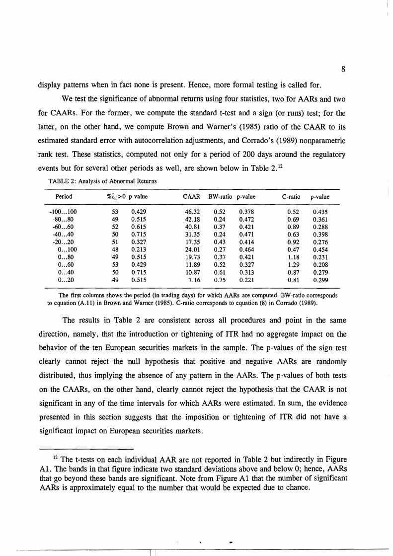
display patterns when in fact none is presento Hence, more formal testing is called foro

We test the significance of abnormal returns using four statistics, two for AARs and two�

for CAARs. For the former, we compute the standard t-test and a sign (or runs) test; for the�

latter, on the other hand, we compute Brown and Warner's (1985) ratio of the CAAR to its�

estimated standard error with autocorrelation adjustments, and Corrado's (1989) nonparametric�

rank test. These statistics, computed not only for a period of 200 days around the regulatory�

events but for several other periods as well, are shown below in Table 2. 12�

TABLE 2: Analysis of Abnormal Returns

Period %fil>O p-value CAAR BW-ratio p-value C-ratio p-value

-100... 100 53 0.429 46.32 0.52 0.378 0.52 0.435� -80... 80 49 0.515 42.18 0.24 0.472 0.69 0.361� -60...60 52 0.615 40.81 0.37 0.421 0.89 0.288� -40.. .40 50 0.715 31.35 0.24 0.471 0.63 0.398� -20...20 51 0.327 17.35 0.43 0.414 0.92 0.276�

0... 100 48 0.213 24.01 0.27 0.464 0.47 0.454� 0... 80 49 0.515 19.73 0.37 0.421 1.18 0.231� 0...60 53 0.429 11.89 0.52 0.327 1.29 0.208� 0.. .40 50 0.715 10.87 0.61 0.313 0.87 0.279� 0...20 49 0.515 7.16 0.75 0.221 0.81 0.299�

The first columns shows the period (in trading days) for which AARs are computed. BW-ratio corresponds to equation (A.U) in Brown and Warner (1985). C-ratio corresponds to equation (8) in Corrado (1989).

The results in Table 2 are consistent across all procedures and point in the same�

direction, namely, that the introduction or tightening of ITR had no aggregate impact on the�

behavior of the ten European securities markets in the sample. The p-values of the sign test�

clearly cannot reject the null hypothesis that positive and negative AARs are randomly�

distributed, thus implying the absence of any pattern in the AARs. The p-values of both tests�

on the CAARs, on the other hand, clearly cannot reject the hypothesis that the CAAR is not�

significant in any of the time intervals for which AARs were estimated. In sum, the evidence�

presented in this section suggests that the imposition or tightening of ITR did not have a�

significant impact on European securities markets.�

12 The t-tests on each individual AAR are not reported in Table 2 but indirectIy in Figure� Al. The bands in that figure indicate two standard deviations above and below O; hence, AARs� that go beyond these bands are significant. Note from Figure Al that the number of significant� AARs is approximately equal to the number that would be expected due to chance.�

.. _-_._---_._-----------,--,------------------------- ._--­

9

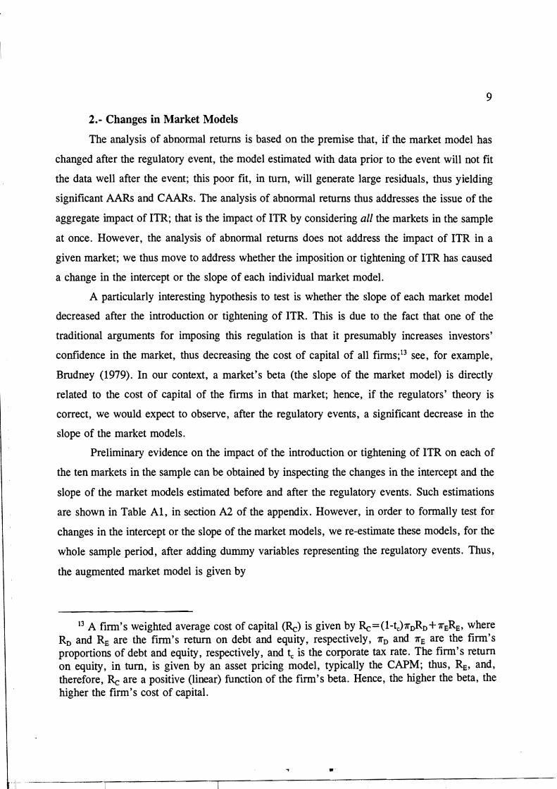
2.- Changes in Market Models

The analysis of abnormal returns is based on the premise that, if the market model has

changed after the regulatory event, the model estimated with data prior to the event will not fit

the data well after the event; this poor fit, in tum, will generate large residuals, thus yielding

significant AARs and CAARs. The analysis of abnormal retums thus addresses the issue of the

aggregate impact of ITR; that is the impact of ITR by considering al! the markets in the sample

at once. However, the analysis of abnormal returns does not address the impact of ITR in a

given market; we thus move to address whether the imposition or tightening of ITR has caused

a change in the intercept or the slope of each individual market model.

A particularly interesting hypothesis to test is whether the slope of each market model

decreased after the introduction or tightening of ITR. This is due to the fact that one of the

traditional arguments for imposing this regulation is that it presumably increases investors'

confidence in the market, thus decreasing the cost of capital of aH firms;13 see, for example,

Brudney (1979). In our context, a market's beta (the slope of the market model) is directly

related to the cost of capital of the firms in that market; hence, if the regulators' theory is

correct, we would expect to observe, after the regulatory events, a significant decrease in the

slope of the market models.

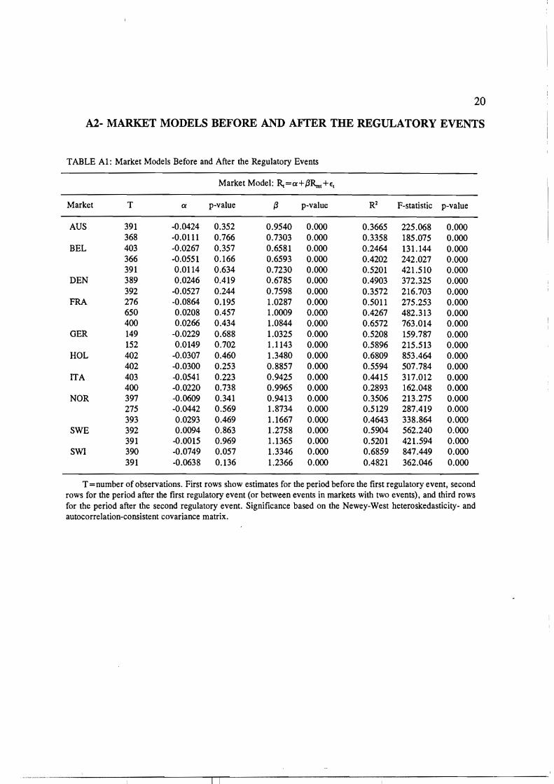
Preliminary evidence on the impact of the introduction or tightening of ITR on each of

the ten markets in the sample can be obtained by inspecting the changes in the intercept and the

slope of the market models estimated before and after the regulatory events. Such estimations

are shown in Table Al, in section A2 of the appendix. However, in order to formaHy test for

changes in the intercept or the slope of the market models, we re-estimate these models, for the

whole sample period, after adding dummy variables representing the regulatory events. Thus,

the augmented market model is given by

13 A firm's weighted average cost of capital (Re) is given by Re=(l-te)7rDRD+7rERE' where Ro and RE are the firm's retum on debt and equity, respectively, 7ro and 7rE are the firm's proportions of debt and equity, respectively, and te is the corporate tax rate. The firm's retum on equity, in tum, is given by an asset pricing model, typically the CAPM; thus, RE' and, therefore, Re are a positive (linear) function of the firm's beta. Hence, the higher the beta, the higher the firm's cost of capital.

., 11­

--------_._-.,-----------,-----------------­

i

i

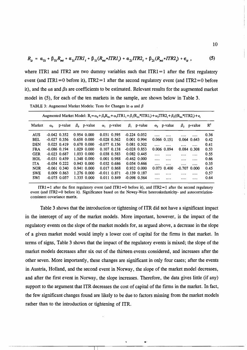
10

where ITRi and ITR2 are two dummy variables such that ITRi = 1 after the first regulatory

event (and ITRi=O before it), ITR2=l after the second regulatory event (and ITR2=O before

it), and the as and {3s are coefficients to be estimated. Relevant results for the augmented market

model in (5), for each of the ten markets in the sample, are shown below in Table 3.

TABLE 3: Augmented Market Models: Tests for Changes in cx and {3

Augmented Market Model: R.. = CXo +{3oR.n, +cx ¡ITR1, +{3¡ (Rm,"'ITR1J+cx2ITRl, +{32«R.n,"'ITRlJ +E,

Market CXo p-value {3o p-value CXl p-value {3¡ p-value CX2 p-value {32 p-value R2

AUS -0.042 0.352 0.954 0.000 0.031 0.595 -0.224 0.032 0.36 BEL -0.027 0.356 0.658 0.000 -0.028 0.562 0.001 0.994 0.066 0.151 0.064 0.643 0.42 DEN 0.025 0.419 0.678 0.000 -0.077 0.156 0.081 0.302 0.41 FRA -0.086 0.194 1.029 0.000 0.107 0.138 -0.028 0.853 0.006 0.894 0.084 0.308 0.53 GER -0.023 0.687 1.033 0.000 0.038 0.583 0.082 0.445 0.55 HüL -0.031 0.459 1.348 0.000 0.001 0.988 -0.462 0.000 0.66 ITA -0.054 0.222 0.943 0.000 0.032 0.686 0.054 0.666 0.35 NüR -0.061 0.340 0.941 0.000 0.017 0.868 0.932 0.000 0.073 0.400 -0.707 0.000 0.45 SWE 0.009 0.863 1.276 0.000 -0.011 0.871 -0.139 0.187 0.57 SWI -0.075 0.057 1.335 0.000 0.011 0.849 -0.098 0.564 0.64

ITR1 = 1 after the first regulatory event (and ITRl =0 before it), and ITRl = 1 after the second regulatory event (and ITRl=O before it). Significance based on the Newey-West heteroskedasticity- and autocorrelation­consistent covariance matrix.

Table 3 shows that the introduction or tightening of ITR did not have a significant impact

in the intercept of any of the market models. More important, however, is the impact of the

regulatory events on the slope of the market models for, as argued above, a decrease in the slope

of a given market model would imply a lower cost of capital for the firms in that market. In

terms of signs, Table 3 shows that the impact of the regulatory events is mixed; the slope of the

market models decreases after six out of the thirteen events considered, and increases after the

other seven. More importantly, these changes are significant in only four cases; after the events

in Austria, Holland, and the second event in Norway, the slope of the market model decreases,

and after the first event in Norway, the slope increases. Therefore, the data gives Httle (if any)

support to the argument that ITR decreases the cost of capital of the firms in the market. In fact,

the few significant changes found are likely to be due to factors missing from the market models

rather than to the introduction or tightening of ITR.

..�

11

The impact of ITR on the intercept and the slope of each market model is also important

to determine whether the series of residuals for each market should be generated by one market

mode1 estimated for the whole sample, or by market models estimated for each subsample. If

individual and joint tests of significance fail to reject the hypothesis of no change in the

coefficients of a market model after the regulatory event (or events), then one market model can

be estimated for the whole sample; this market model would then generate the series of residuals

for that market. If, however, these tests reject the hypothesis of no change in the coefficients,

then one market model would have to be estimated for each subsample, and each market model

would then generate the residuals for each subsample.

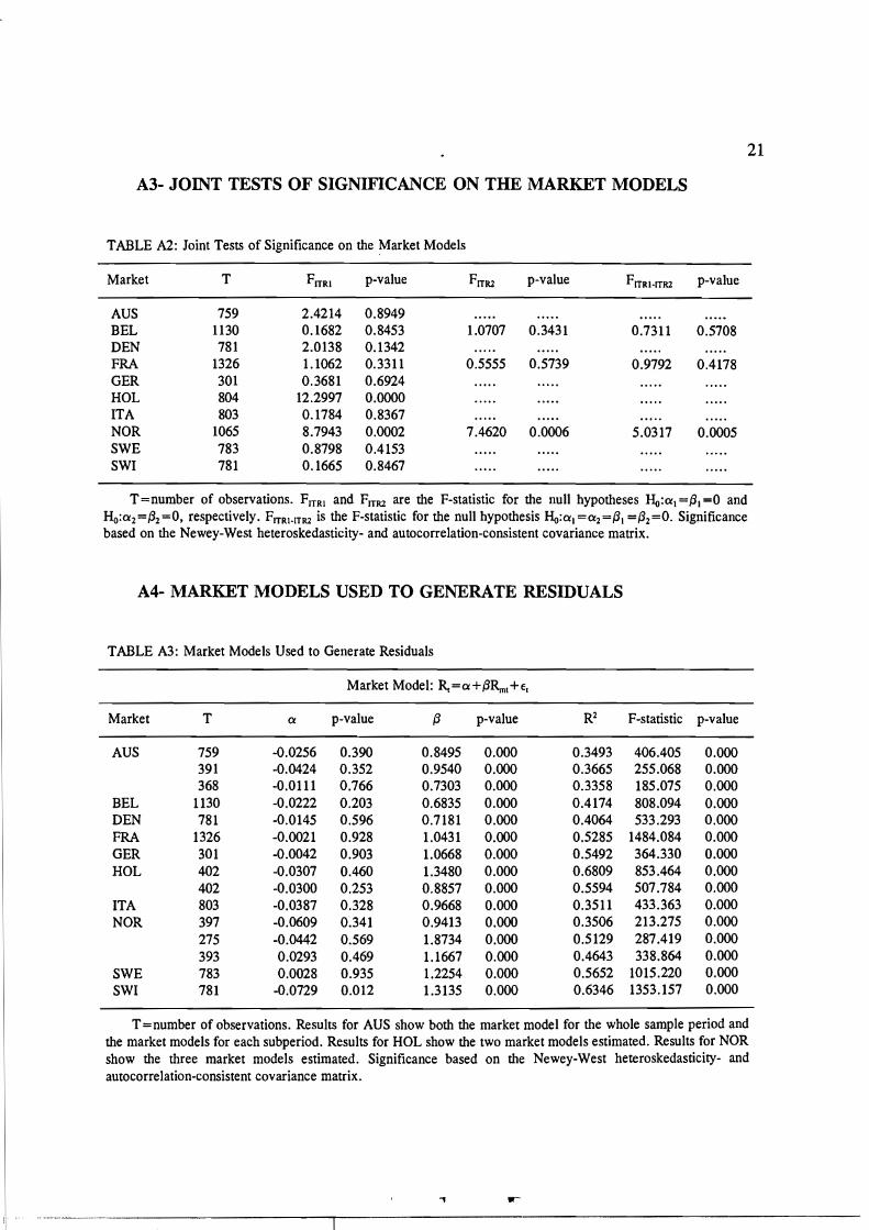
Tests of significance for individual coefficients are shown in Table 3 and were discussed

aboye; joint tests of significance are shown in Table A2, in section A3 of the appendix. These

joint tests show that the market model has changed after on1y three out of the thirteen events

considered; these changes have occurred after the regulatory event in Holland, and after each

of the two regulatory events in Norway. Therefore, two market models are estimated for

Holland (one before and one after the regulatory event), three market models are estimated for

Norway (one before the first regulatory event, one between events, and one after the second

event), and one market model for the rest of the markets in the sample. Note that in the case of

Austria, the t-test on the slope of the market model implies that a significant change occurred

after the regulatory event, but the joint test in Table A2 implies that the market model itself did

not change. Given this contradictory evidence, residuals for Austria are estimated in two ways,

namely, from one market model for the whole sample period, and from two market models (one

for each subsample).14 The market models used to generate the residuals to be used in the

remainder of this study are reported in Table A3, in section A4 of the appendix.

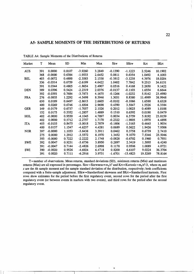
3.- Changes in Mean Returns and Volatility

Several relevant characteristics of the distribution of retums generated by the market

models reported in Table A3 are reported in Table A4, in section A5 of the appendix. This table

14 All results to be reported for Austria correspond to the series of residuals generated by two market models; these results are virtually identical to those for the series of residuals generated by one market model for the whole sample.

~-~~--~~----_.._-----------r--------------------­

12

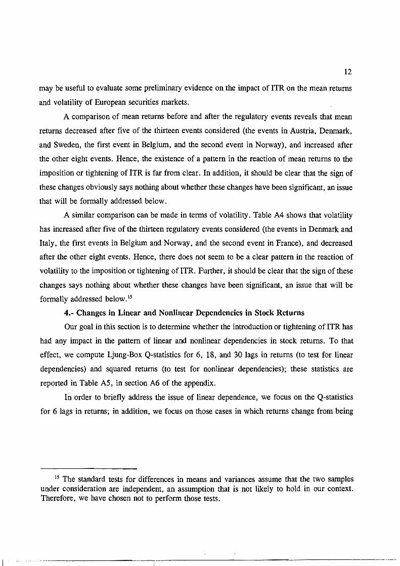
may be useful to evaluate sorne preliminary evidence on the impact of ITR on the mean returns

and volatility of European securities markets.

A comparison of mean returns before and after the regulatory events reveals that mean

returns decreased after five of the thirteen events considered (the events in Austria, Denmark,

and Sweden, the first event in Belgium, and the second event in Norway), and increased after

the other eight events. Hence, the existence of a pattern in the reaction of mean returns to the

imposition or tightening of ITR is far from clear. In addition, it should be clear that the sign of

these changes obviously says nothing about whether these changes have been significant, an issue

that will be formally addressed below.

A similar comparison can be made in terms of volatility. Table A4 shows that volatility

has increased after five of the thirteen regulatory events considered (the events in Denmark and

Italy, the first events in Belgium and Norway, and the second event in France), and decreased

after the other eight events. Hence, there does not seem to be a clear pattern in the reaction of

volatility to the imposition or tightening of ITR. Further, it should be clear that the sign of these

changes says nothing about whether these changes have been significant, an issue that will be

formally addressed below. 15

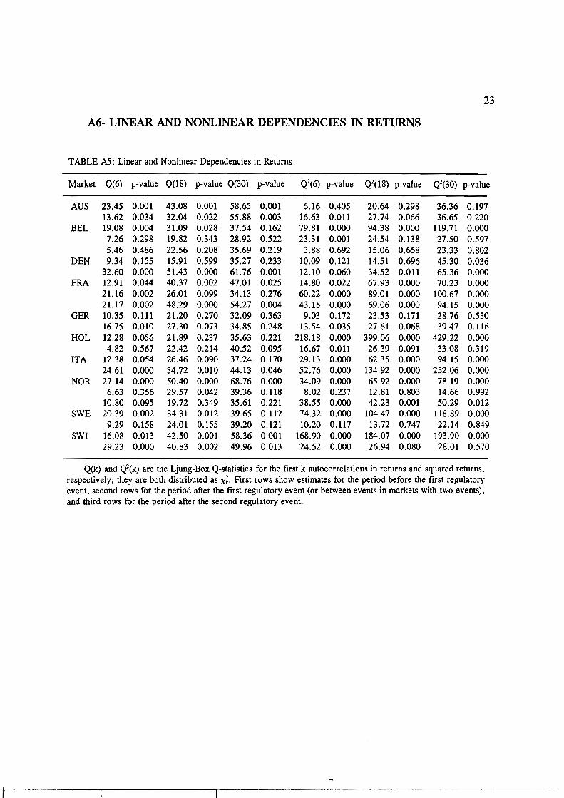
4.- Changes in Linear and Nonlinear Dependencies in Stock Returns

Our goal in this section is to determine whether the introduction or tightening of ITR has

had any impact in the pattern of linear and nonlinear dependencies in stock returns. To that

effect, we compute Ljung-Box Q-statistics for 6, 18, and 30 lags in returns (to test for linear

dependencies) and squared returns (to test for nonlinear dependencies); these statistics are

reported in Table AS, in section A6 of the appendix.

In order to briefly address the issue of linear dependence, we focus on the Q-statistics

for 6 lags in returns; in addition, we focus on those cases in which returns change from being

15 The standard tests for differences in means and variances assume that the two samples under consideration are independent, an assumption that is not likely to hold in our context. Therefore, we have chosen not to perform those tests.

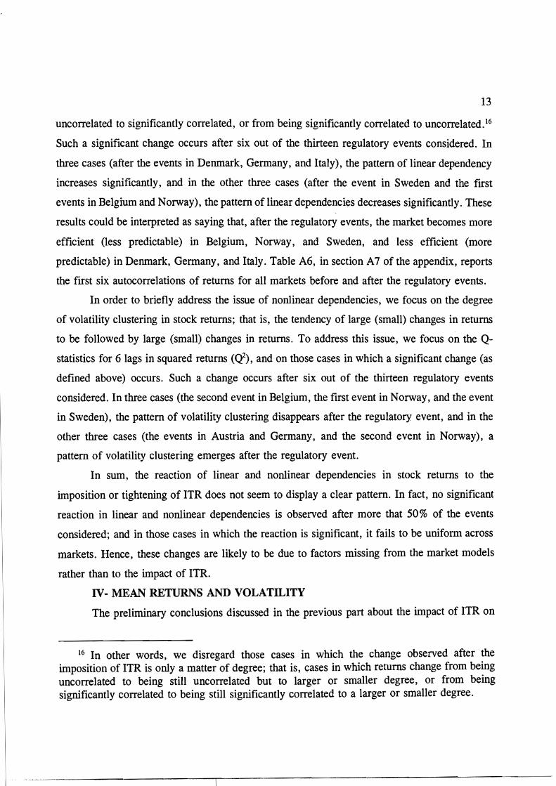
13

uncorrelated to significantly correlated, or from being significantly correlated to uncorrelated. 16

Such a significant change occurs after six out of the thirteen regulatory events considered. In

three cases (after the events in Denmark, Germany, and Italy), the pattern of linear dependency

increases significantly, and in the other three cases (after the event in Sweden and the first

events in Belgium and Norway), the pattern of linear dependencies decreases significantly. These

results could be interpreted as saying that, after the regulatory events, the market becomes more

efficient (less predictable) in Belgium, Norway, and Sweden, and less efficient (more

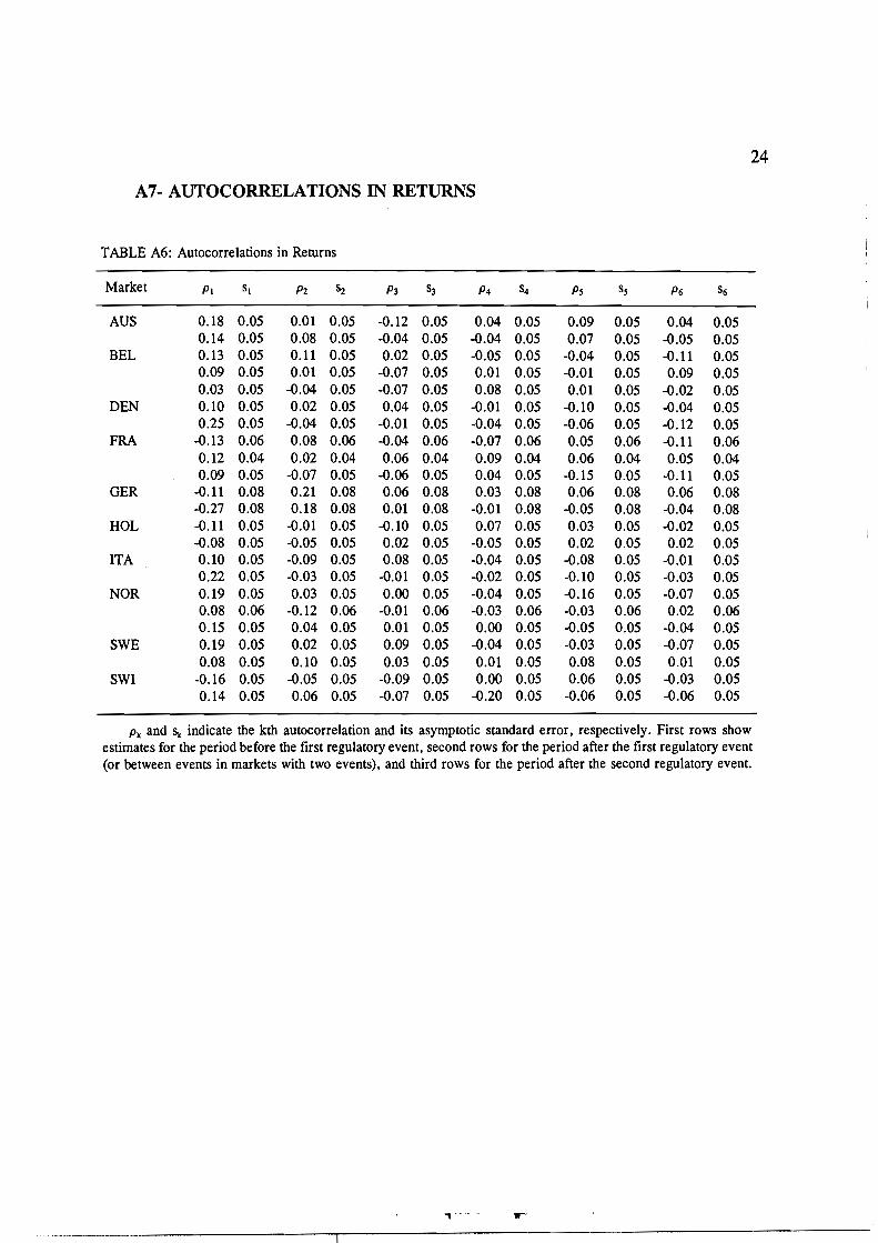
predictable) in Denmark, Germany, and Italy. Table A6, in section A7 of the appendix, reports

the first six autocorrelations of returns for all markets before and after the regulatory events.

In order to briefly address the issue of nonlinear dependencies, we focus on the degree

of volatility clustering in stock returns; that is, the tendency of large (small) changes in returns

to be followed by large (small) changes in returns. To address this issue, we focus on the Q­

statistics for 6 lags in squared returns (Q2), and on those cases in which a significant change (as

defined above) occurs. Such a change occurs after six out of the thirteen regulatory events

considered. In three cases (the second event in Belgium, the first event in Norway, and the event

in Sweden), the pattern of volatility clustering disappears after the regulatory event, and in the

other three cases (the events in Austria and Germany, and the second event in Norway), a

pattern of volatility clustering emerges after the regulatory evento

In sum, the reaction of linear and nonlinear dependencies in stock returns to the

imposition or tightening of ITR does not seem to display a clear pattern. In fact, no significant

reaction in linear and nonlinear dependencies is observed after more that 50% of the events

considered; and in those cases in which the reaction is significant, it fails to be uniform across

markets. Hence, these changes are likely to be due to factors missing from the market models

rather than to the impact of ITR.

IV- MEAN RETURNS AND VOLATILITY

The preliminary conclusions discussed in the previous part about the impact of ITR on

16 In other words, we disregard those cases in which the change observed after the imposition of ITR is only a matter of degree; that is, cases in which returns change from being uncorrelated to being still uncorrelated but to larger or smaller degree, or from being significantly correlated to being still significantly correlated to a larger or smaller degree.

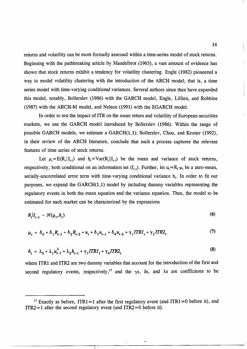
14

retums and volatility can be more formally assessed within a time-series model of stock retums.�

Beginning with the pathbreaking article by Mandelbrot (1963), a vast amount of evidence has�

shown that stock retums exhibit a tendency for volatility clustering. Engle (1982) pioneered a�

way to model volatility clustering with the introduction of the ARCH model; that is, a time�

series model with time-varying conditional variances. Several authors since then have expanded�

this model, notably, Bollerslev (1986) with the GARCH model, Engle, Lillien, and Robbins�

(1987) with the ARCH-M model, and Nelson (1991) with the EGARCH model.�

In order to test the impact of ITR on the mean retum and volatility of European securities�

markets, we use the GARCH model introduced by Bollerslev (1986). Within the range of�

possible GARCH models, we estimate a GARCH(1,I); Bollerslev, Chou, and Kroner (1992),�

in their review of the ARCH literature, conclude that such a process captures the relevant�

features of time series of stock retums.�

Let 1L¡=E(RIII¡_I) and hl=Var(~III_1) be the mean and variance of stock retums,�

respectively, both conditional on an information set (I¡-I). Further, let U¡=~-IL¡ be a zero-mean,�

serially-uncorrelated error term with time-varying conditional variance h¡. In order to fit our�

purposes, we expand the GARCH(1, 1) model by including dummy variables representing the�

regulatory events in both the mean equation and the variance equation. Thus, the model to be�

estimated for each market can be characterized by the expressions�

(6)

(7)

(8)

where ITRl and ITR2 are two dummy variables that account for the introduction of the first and

second regulatory events, respectively, 17 and the 'YS, oS, and AS are coefficients to be

17 Exactly as before, ITRl = 1 after the first regulatory event (and ITRl =0 before it), and� ITR2= 1 after the second regulatory event (and ITR2=O before it).�

--------- -------------,.......,.--------------------------­

15

estimated. 18 As in Akgiray (l989), among several others, we assume that ull Iloh and, therefore,

R¡ I11-1, are normally distributed with mean O and variance l\.

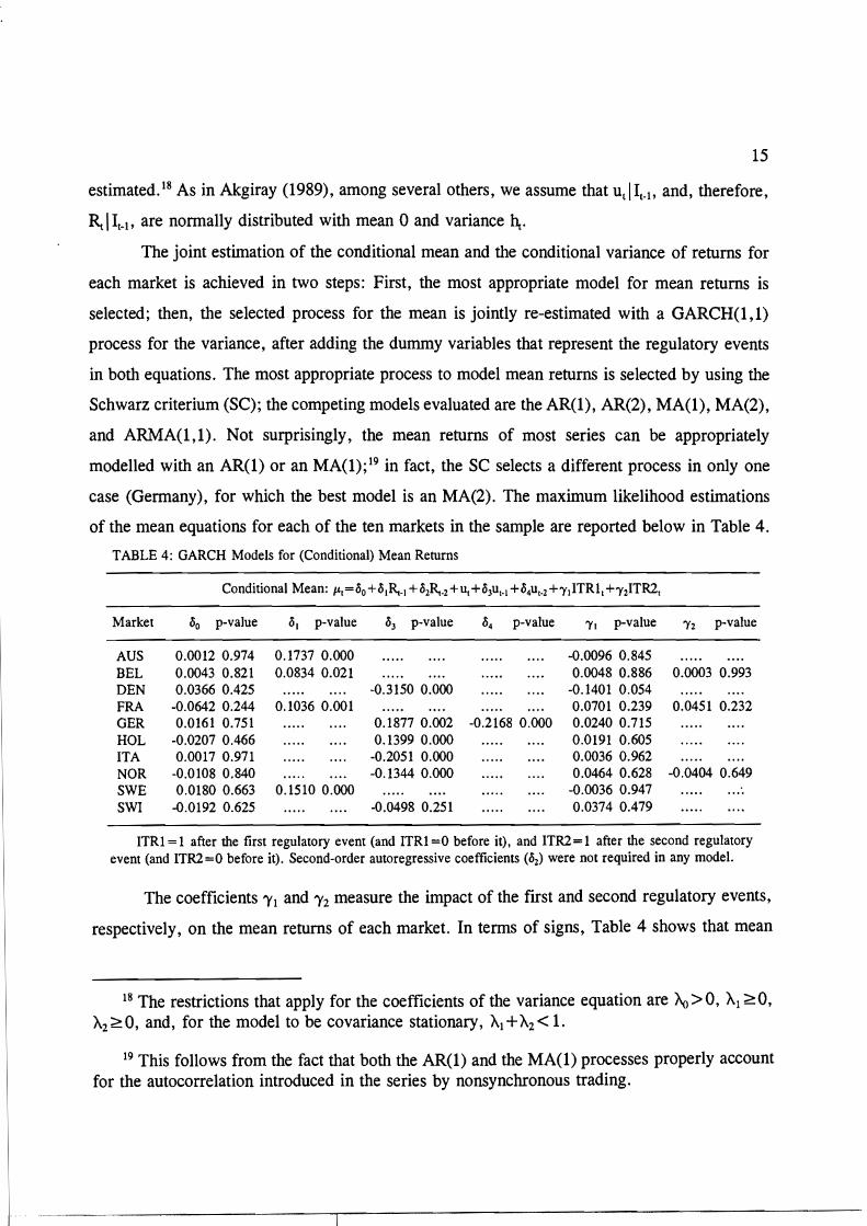
The joint estimation of the conditional mean and the conditional variance of retums for

each market is achieved in two steps: First, the most appropriate model for mean retums is

selected; then, the selected process for the mean is jointly re-estimated with a GARCH(l, 1)

process for the variance, after adding the dummy variables that represent the regulatory events

in both equations. The most appropriate process to model mean retums is selected by using the

Schwarz criterium (SC); the competing models evaluated are the AR(I), AR(2), MA(I), MA(2),

and ARMA(l,I). Not surprisingly, the mean retums of most series can be appropriately

modelled with an AR(l) or an MA(l);19 in fact, the SC selects a different process in only one

case (Germany), for which the best model is an MA(2). The maximum likelihood estimations

of the mean equations for each of the ten markets in the sample are reported below in Table 4.

TABLE 4: GARCH Models for (Conditional) Mean Returns

Market ¿¡o p-value ¿¡¡ p-value ¿¡3 p-value ¿¡4 p-value 'YI p-value 'Y2 p-value

AUS 0.0012 0.974 0.1737 0.000 -0.0096 0.845 BEL 0.0043 0.821 0.0834 0.021 0.0048 0.886 0.0003 0.993 DEN 0.0366 0.425 -0.3150 0.000 -0.1401 0.054 FRA -0.0642 0.244 0.1036 0.001 0.0701 0.239 0.0451 0.232 GER 0.0161 0.751 0.1877 0.002 -0.2168 0.000 0.0240 0.715 HOL -0.0207 0.466 0.1399 0.000 0.0191 0.605 ITA 0.0017 0.971 -0.2051 0.000 0.0036 0.962 NOR -0.0108 0.840 -0.1344 0.000 0.0464 0.628 -0.0404 0.649 SWE 0.0180 0.663 0.1510 0.000 -0.0036 0.947 .... SWI -0.0192 0.625 -0.0498 0.251 0.0374 0.479

ITRl = 1 after the first regulatory event (and ITRl =0 before it), and ITR2 = 1 after the seeond regulatory event (and ITR2=O before it). Seeond-order autoregressive eoefficients (¿¡2) were not required in any model.

The coefficients 1'1 and 1'2 measure the impact of the first and second regulatory events,

respectively, on the mean retums of each market. In terms of signs, Table 4 shows that mean

18 The restrictions that apply for the coefficients of the variance equation are Ao> O, Al ~ O, A2 ~ O, and, for the model to be covariance stationary, Al +A2 < 1.

19 This follows from the fact that both the AR(I) and the MA(l) processes properly account for the autocorrelation introduced in the series by nonsynchronous trading.

16

returns have decreased (1'1 <O or 1'2<0) after four events (those in Austria, Denmark, and

Sweden, and the second event in Norway), and increased (1'1>0 or 1'2>0) after the other nine

events. Far more important, however, is the fact that none of these coefficients is significant;

that is, the evidence shows that the imposition or tightening of ITR did not have any significant

impact on the mean returns of any of the markets in the sample.

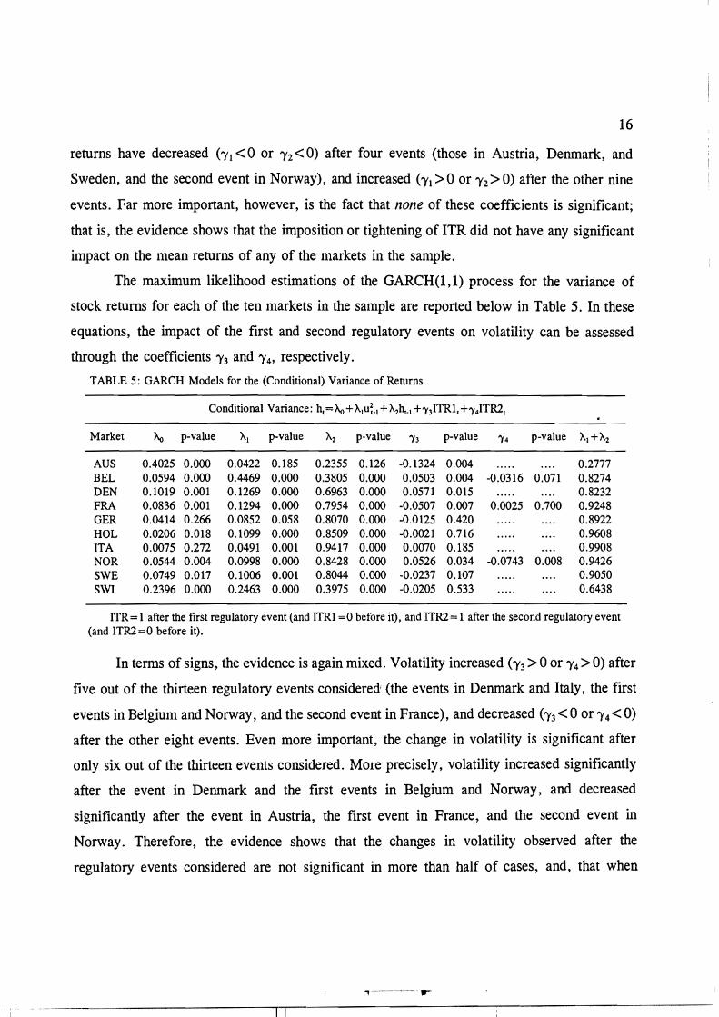
The maximum likelihood estimations of the GARCH(1,1) process for the variance of

stock returns for each of the ten markets in the sample are reported below in Table 5. In these

equations, the impact of the first and second regulatory events on volatility can be assessed

through the coefficients 1'3 and 1'4' respectively.

TABLE 5: GARCR Models for the (Conditional) Variance of Returns

Conditional Variance: hl=Aa+A1U~.• +A2h,.• +'Y3ITRl,+'Y4ITR2,

Market Aa p-value Al p-value A2 p-value 'Y3 p-value 'Y4 p-value A¡+A2

AUS 0.4025 0.000 0.0422 0.185 0.2355 0.126 -0.1324 0.004 0.2777 BEL 0.0594 0.000 0.4469 0.000 0.3805 0.000 0.0503 0.004 -0.0316 0.071 0.8274 DEN 0.1019 0.001 0.1269 0.000 0.6963 0.000 0.0571 0.015 0.8232 FRA 0.0836 0.001 0.1294 0.000 0.7954 0.000 -0.0507 0.007 0.0025 0.700 0.9248 GER 0.0414 0.266 0.0852 0.058 0.8070 0.000 -0.0125 0.420 0.8922 ROL 0.0206 0.018 0.1099 0.000 0.8509 0.000 -0.0021 0.716 0.9608 ITA 0.0075 0.272 0.0491 0.001 0.9417 0.000 0.0070 0.185 0.9908 NOR 0.0544 0.004 0.0998 0.000 0.8428 0.000 0.0526 0.034 -0.0743 0.008 0.9426 SWE 0.0749 0.017 0.1006 0.001 0.8044 0.000 -0.0237 0.107 0.9050 SWI 0.2396 0.000 0.2463 0.000 0.3975 0.000 -0.0205 0.533 0.6438

ITR= 1 after the first regulatory event (and ITRl =0 before it), and ITR2= 1 after the second regulatory evem (and ITR2=O before it).

In terms of signs, the evidence is again mixed. Volatility increased (1'3> Oor 1'4> O) after

five out of the thirteen regulatory events consideredi (the events in Denmark and Italy, the first

events in Belgium and Norway, and the second event in France), and decreased (1'3 <Oor 1'4< O)

after the other eight events. Even more important, the change in volatility is significant after

only six out of the thirteen events considered. More precisely, volatility increased significantly

after the event in Denmark and the first events in Belgium and Norway, and decreased

significantly after the event in Austria, the first event in France, and the second event in

Norway. Therefore, the evidence shows that the changes in volatility observed after the

regulatory events considered are not significant in more than half of cases, and, that when

...__._._-----------,-¡-'-----------:------------­

17

significant changes are observed, no clear pattern in the changes emerges. Hence, the significant

changes in volatility observed are likely to be due to the impact of factors missing from the

model rather than to the impact of ITR.

V- CONCLUSIONS

During the last thirty years, a vast literature has considered the issue of insider trading�

and has evaluated the theoretical benefits and costs of regulating this activity. In this article, we�

have attempted to evaluate the empirical impact of ITR by focussing on the regulations imposed�

between 1988 and 1994 in ten European securities markets.�

Most of the evidence analyzed in this article points in the same direction; that is, to the

fact that ITR has had little, if any, impact on the securities markets analyzed. The analysis of

abnormal returns failed to detect an aggregate impact of ITR when considering a11 the markets

in the sample at once. Individual and joint tests of significance on the market models, on the

other hand, detected significant changes after the regulatory events in very few cases. In

particular, the argument that ITR decreases the cost of capital of the firms in the market was

seriously questioned by the evidence. And very few significant changes in the pattern of linear

and nonlinear dependencies in stock returns occurred after the regulatory events.

The results of the GARCH models estimated to test the impact of ITR on mean returns

and volatility were also consistent with the previous results. In particular, the evidence showed

that the imposition or tightening of ITR did not have a significant impact on mean returns in any

of the markets in the sample. The evidence also showed that over 50% of the regulatory events

considered did not have a significant impact on volatility, and that in those cases in which the

events did have a significant impact, no clear pattern in the reaction of volatility emerged.

Therefore, as argued aboye, we are inclined to think that the significant changes we detected in

the market models, in the pattern of linear and nonlinear dependencies, and in volatility are

likely to be due to the impact of factors missing from the estimated models rather than to the

impact of ITR.

We prefer not to draw hard conclusions at this point about the reasons for which

investors in European securities markets have virtua11y ignored insider trading restrictions. The

., .

.•.......•.._---------_._---,------------------------­

18

issue of enforcement, however, irnmediately comes to mind.20 Casual empiricism suggests that

very few resources are a1located in European markets to detect the presence of insiders; although

we have no hard data to back this hypothesis, scattered evidence seems to point in this direction.

It is thus natural to wonder, if the previous speculation is accepted, why monitoring is so laxo

After a1l, is it reasonable to waste resources in discussing and writing a regulation that is later

going to be virtua1ly ignored?

One reason behind the lack of enforcement may be that insider trading is not considered

so hannful in Europe as it is in the United States. In many European countries, notably in

Gennany, insider trading is considered as a part of doing business; see, for example, Standen

(1995). It may be the case that European countries fina1ly capitulated to the demands of the SEC

and decided to impose ITR; but not being fu1ly convinced that imposing ITR was the right thing

to do, they put very Httle effort in enforcing this regulation. We obviously cannot back this

speculation with hard data; but we can certain1y argue, with the evidence we do have, that

European markets have virtua1ly ignored the restrictions on insider trading imposed in recent

years.

20 Directive 89/592/EEC, issued by the Council ofthe European Cornmunities on November� 13, 1989, provided that member states had to regulate insider trading, according to the� guidelines given in the Directive, before June 1, 1992. However, the Directive did not create� a central agency with the purpose of enforcing compliance; it merely provided that member� states had to designate authorities responsible for the proper application of the insider trading� prohibitions, and that these authorities were to be granted the necessary supervisory and� investigative powers.�

._._._._-------------,--¡----------------------- ,---­

19

APPENDIX

Al- ANALYSIS OF ABNORMAL RETURNS

FIGURE A1: AVERAGE ABNORMAL RETURNS

10 .o tO .o

III .,.l: L.. .o:1...., V

c:: N .o"O E oL.. o ci l: I .n « N

Ql O� O'� I O Ql> , L..

O"'" «

lO

O I

ro O I -120 -so -40 o 40 80 120

Days

FIGURE A2: CUMULATIVE AVERAGE ABNORMAL RETURNS lll.----..---r---........-"'T"""-.......--r---.--"""T'"-.....,...--,----...---.�

~ L_-1-20.........--_.i..80---'---_..J.4-0--'--...J0l.-----J'---4LO-----'---s.i..0---'-----'120�

Doys

.-----.-----------.-----r--.-------------------------­

20

A2- MARKET MODELS BEFORE AND AFTER THE REGULATORY EVENTS

TABLE Al: Market Models Before and After the Regulatory Events

Market Model: ~=a+¡3Rnt+EI

Market T a p-value ¡3 p-value R2 F-statistic p-value

AUS 391 -0.0424 0.352 0.9540 0.000 0.3665 225.068 0.000 368 -0.0111 0.766 0.7303 0.000 0.3358 185.075 0.000

BEL 403 -0.0267 0.357 0.6581 0.000 0.2464 131.144 0.000 366 -0.0551 0.166 0.6593 0.000 0.4202 242.027 0.000 391 0.0114 0.634 0.7230 0.000 0.5201 421.510 0.000

DEN 389 0.0246 0.419 0.6785 0.000 0.4903 372.325 0.000 392 -0.0527 0.244 0.7598 0.000 0.3572 216.703 0.000

FRA 276 -0.0864 0.195 1.0287 0.000 0.5011 275.253 0.000 650 0.0208 0.457 1.0009 0.000 0.4267 482.313 0.000 400 0.0266 0.434 1.0844 0.000 0.6572 763.014 0.000

GER 149 -0.0229 0.688 1.0325 0.000 0.5208 159.787 0.000 152 0.0149 0.702 1.1143 0.000 0.5896 215.513 0.000

HüL 402 -0.0307 0.460 1.3480 0.000 0.6809 853.464 0.000 402 -0.0300 0.253 0.8857 0.000 0.5594 507.784 0.000

ITA 403 -0.0541 0.223 0.9425 0.000 0.4415 317.012 0.000 400 -0.0220 0.738 0.9965 0.000 0.2893 162.048 0.000

NüR 397 -0.0609 0.341 0.9413 0.000 0.3506 213.275 0.000 275 -0.0442 0.569 1.8734 0.000 0.5129 287.419 0.000 393 0.0293 0.469 1.1667 0.000 0.4643 338.864 0.000

SWE 392 0.0094 0.863 1.2758 0.000 0.5904 562.240 0.000 391 -0.0015 0.969 1.1365 0.000 0.5201 421.594 0.000

SWI 390 -0.0749 0.057 1.3346 0.000 0.6859 847.449 0.000 391 -0.0638 0.136 1.2366 0.000 0.4821 362.046 0.000

T =number of observations. First rows show estimates for the period before the first regulatory event, second rows for the period after the first regulatory event (or between events in markets with two events), and third rows for the period after the second regulatory evento Significance based on the Newey-West heteroskedasticity- and autocorrelation-consistent covariance matrix.

------.-------------------r-r---------------------------­

21

A3- JOINT TESTS OF SIGNIFICANCE ON THE MARKET MODELS

TABLE A2: Joint Tests of Significance on the Market Models

Market T FITRI p-value F1TR2 p-value FITRI.ITR2 p-value

AUS 759 2.4214 0.8949 BEL 1130 0.1682 0.8453 1.0707 0.3431 0.7311 0.5708 DEN 781 2.0138 0.1342 FRA 1326 1.1062 0.3311 0.5555 0.5739 0.9792 0.4178 GER 301 0.3681 0.6924 HOL 804 12.2997 0.0000 ITA 803 0.1784 0.8367 NOR 1065 8.7943 0.0002 7.4620 0.0006 5.0317 0.0005 SWE 783 0.8798 0.4153 SWI 781 0.1665 0.8467

T=number of observations. F1TR1 and FITR2 are the F-statistic for the null hypotheses Ho:a l =,81 =0 and HO:a2=,82=0, respectively. FITRI.ITR2 is the F-statistic for the null hypothesis Ho:al=a2=,81 =,82=0. Significance based on the Newey-West heteroskedasticity- and autocorrelation-consistent covariance matrix.

A4- MARKET MODELS USED TO GENERATE RESIDUALS

TABLE A3: Market Models Used to Generate Residuals

Market Model: R,=a+,8Roll +f,

Market T a p-value ,8 p-value R2 F-statistic p-value

AUS� 759 -0.0256 0.390 0.8495 0.000 0.3493 406.405 0.000 391 -0.0424 0.352 0.9540 0.000 0.3665 255.068 0.000 368 -0.0111 0.766 0.7303 0.000 0.3358 185.075 0.000

BEL 1130 -0.0222 0.203 0.6835 0.000 0.4174 808.094 0.000 DEN 781 -0.0145 0.596 0.7181 0.000 0.4064 533.293 0.000 FRA 1326 -0.0021 0.928 1.0431 0.000 0.5285 1484.084 0.000 GER 301 -0.0042 0.903 1.0668 0.000 0.5492 364.330 0.000 HOL 402 -0.0307 0.460 1.3480 0.000 0.6809 853.464 0.000

402 -0.0300 0.253 0.8857 0.000 0.5594 507.784 0.000 ITA 803 -0.0387 0.328 0.9668 0.000 0.3511 433.363 0.000 NOR 397 -0.0609 0.341 0.9413 0.000 0.3506 213.275 0.000

275 -0.0442 0.569 1.8734 0.000 0.5129 287.419 0.000 393 0.0293 0.469 1.1667 0.000 0.4643 338.864 0.000

SWE 783 0.0028 0.935 1.2254 0.000 0.5652 1015.220 0.000 SWI 781 -0.0729 0.012 1.3135 0.000 0.6346 1353.157 0.000

T=number of observations. Results for AUS show both the market model for the whole sample period and the market models for each subperiod. Results for HOL show the two market models estimated. Results for NOR show the three market models estimated. Significance based on the Newey-West heteroskedasticity- and autocorrelation-consistent covariance matrix.

, Ir'

------------------------""T-----------.-------------------­

22

A5- SAMPLE MOMENTS OF THE DISTRIBUTIONS OF RETURNS

TABLE A4: Sample Moments of the Distributions of Returns

Market T Mean SD Min Max Skw SSkw Krt SKrt

AUS 391 0.0000 0.8107 -3.9260 3.2849 -0.1390 -1.1223 2.5246 10.1902 368 -0.0000 0.6384 -1.9533 2.6452 0.0811 0.6354 1.0492 4.1083

BEL 403 -0.0072 0.4800 -2.3583 2.1338 -0.3812 -3.1238 4.3976 18.0204 336 -0.0314 0.6759 -2.6199 4.6422 1.0402 7.7842 9.2513 34.6151 391 0.0344 0.4805 -1.8654 2.4907 0.0516 0.4168 2.2650 9.1422

DEN 389 0.0396 0.5424 -2.2319 2.0376 -0.0137 -0.1103 1.6554 6.6644 392 -0.0393 0.7684 -3.7873 4.1675 -0.1266 -1.0232 5.8142 23.4980

FRA 276 -0.0835 1.2292 -4.5498 8.3946 1.3031 8.8380 11.4989 38.9948 650 0.0189 0.6497 -2.8613 2.6605 -0.0102 -0.1066 1.6588 8.6328 400 0.0269 0.6746 -1.6504 2.9698 0.4390 3.5847 1.5526 6.3384

GER 149 -0.0179 0.6737 -1.7057 2.1526 0.2012 1.0025 0.4089 1.0188 152 0.0175 0.5352 -1.2857 1.4889 0.1310 0.6592 0.0190 0.0479

HOL 402 -0.0000 0.9550 -4.1045 4.7897 0.8034 6.5759 5.8192 23.8159 402 0.0000 0.5712 -2.2757 1.7170 -0.2322 -1.9005 1.0970 4.4898

ITA 403 -0.0155 0.8475 -3.0018 2.7879 -0.1606 -1.3165 0.4645 1.9034 400 0.0157 1.1547 -4.6257 4.4281 0.0689 0.5622 . 1.9426 7.9306

NOR 397 -0.0000 1.1053 -3.6438 3.3911 0.0462 0.3758 0.6739 2.7410 275 0.0000 1.2912 -3.5572 8.1970 1.3452 9.1070 7.5346 25.5046 393 -0.0000 0.7222 -2.2222 2.1748 -0.0828 -0.6702 0.1960 0.7931

SWE 392 0.0047 0.9231 -3.6736 3.8950 0.2897 2.3419 1.5895 6.4240 391 -0.0047 0.7144 -2.4826 2.6998 0.1178 0.9506 1.0089 4.0721

SWI 390 -0.0020 0.9526 -4.6924 6.4718 0.8200 6.6107 9.0224 36.3704 391 0.0020 0.7111 -6.2916 3.9731 -1.6701 -13.4823 19.5269 78.8164

T=number of observations. Mean returns, standard deviations (SD), minimum returns (Min) and maximum returns (Max) are aH expressed in percentages. Skw=Skewness=m3/s

3 and Krt=Kurtosis=mis4-3, where lIl¡ and s are the ith sample moment and the sample standard deviation of the distribution, respectively; both coefficients computed with a finite-sample adjustment. SSkw=Standardized skewness and SKrt=Standardized kurtosis. First rows show estimates for the period before the first regulatory event, second rows for the period after the first regulatory event (or between events in markets with two evems), and third rows for the period after the second regulatory evento

l·· _~----_._--,----------~------------------------------1

23

A6- LINEAR AND NONLINEAR DEPENDENCIES IN RETURNS

TABLE AS: Linear and Nonlinear Dependencies in Returns

Market Q(6) p-value Q(18) p-value Q(30) p-value Q2(6) p-value Q2(18) p-value Q2(30) p-value

AUS 23.45 0.001 43.08 0.001 58.65 0.001 6.16 0.405 20.64 0.298 36.36 0.197 13.62 0.034 32.04 0.022 55.88 0.003 16.63 0.011 27.74 0.066 36.65 0.220

BEL 19.08 0.004 31.09 0.028 37.54 0.162 79.81 0.000 94.38 0.000 119.71 0.000 7.26 0.298 19.82 0.343 28.92 0.522 23.31 0.001 24.54 0.138 27.50 0.597 5.46 0.486 22.56 0.208 35.69 0.219 3.88 0.692 15.06 0.658 23.33 0.802

DEN 9.34 0.155 15.91 0.599 35.27 0.233 10.09 0.121 14.51 0.696 45.30 0.036 32.60 0.000 51.43 0.000 61.76 0.001 12.10 0.060 34.52 0.011 65.36 0.000

FRA 12.91 0.044 40.37 0.002 47.01 0.025 14.80 0.022 67.93 0.000 70.23 0.000 21.16 0.002 26.01 0.099 34.13 0.276 60.22 0.000 89.01 0.000 100.67 0.000 21.17 0.002 48.29 0.000 54.27 0.004 43.15 O.QOO 69.06 0.000 94.15 0.000

GER 10.35 0.111 21.20 0.270 32.09 0.363 9.03 0.172 23.53 0.171 28.76 0.530 16.75 0.010 27.30 0.073 34.85 0.248 13.54 0.035 27.61 0.068 39.47 0.116

HOL 12.28 0.056 21.89 0.237 35.63 0.221 218.18 0.000 399.06 0.000 429.22 0.000 4.82 0.567 22.42 0.214 40.52 0.095 16.67 0.011 26.39 0.091 33.08 0.319

ITA 12.38 0.054 26.46 0.090 37.24 0.170 29.13 0.000 62.35 0.000 94.15 0.000 24.61 0.000 34.72 0.010 44.13 0.046 52.76 0.000 134.92 0.000 252.06 0.000

NOR 27.14 0.000 50.40 0.000 68.76 0.000 34.09 0.000 65.92 0.000 78.19 0.000 6.63 0.356 29.57 0.042 39.36 0.118 8.02 0.237 12.81 0.803 14.66 0.992

10.80 0.095 19.72 0.349 35.61 0.221 38.55 0.000 42.23 0.001 50.29 0.012 SWE 20.39 0.002 34.31 0.012 39.65 0.112 74.32 0.000 104.47 0.000 118.89 0.000

9.29 0.158 24.01 0.155 39.20 0.121 10.20 0.117 13.72 0.747 22.14 0.849 SWI 16.08 0.013 42.50 0.001 58.36 0.001 168.90 0.000 184.07 0.000 193.90 0.000

29.23 0.000 40.83 0.002 49.96 0.013 24.52 0.000 26.94 0.080 28.01 0.570

Q(k) and Q2(k) are the Ljung-Box Q-statistics for the first k autocorrelations in returns and squared returns, respectively; they are both distributed as x~. First rows show estimates for the period before the first regulatory event, second rows for the period after the first regulatory event (or between events in markets with two events). and third rows for the period after the second regulatory evento

........----.--------.------r--------------------------.---­

24

A7- AUTOCORRELATIONS IN RETURNS�

TABLE A6: Autocorrelations in Returns

Market P. s. P2 ~ P3 S3 P4 S4 P5 S5 P6 S6

AUS 0.18 0.05 0.01 0.05 -0.12 0.05 0.04 0.05 0.09 0.05 0.04 0.05 0.14 0.05 0.08 0.05 -0.04 0.05 -0.04 0.05 0.07 0.05 -0.05 0.05

BEL 0.13 0.05 0.11 0.05 0.02 0.05 -0.05 0.05 -0.04 0.05 -0.11 0.05 0.09 0.05 0.01 0.05 -0.07 0.05 0.01 0.05 -0.01 0.05 0.09 0.05 0.03 0.05 -0.04 0.05 -0.07 0.05 0.08 0.05 0.01 0.05 -0.02 0.05

DEN 0.10 0.05 0.02 0.05 0.04 0.05 -0.01 0.05 -0.10 0.05 -0.04 0.05 0.25 0.05 -0.04 0.05 -0.01 0.05 -0.04 0.05 -0.06 0.05 -0.12 0.05

FRA -0.13 0.06 0.08 0.06 -0.04 0.06 -0.07 0.06 0.05 0.06 -0.11 0.06 0.12 0.04 0.02 0.04 0.06 0.04 0.09 0.04 0.06 0.04 0.05 0.04 0.09 0.05 -0.07 0.05 -0.06 0.05 0.04 0.05 -0.15 0.05 -0.11 0.05

GER -0.11 0.08 0.21 0.08 0.06 0.08 0.03 0.08 0.06 0.08 0.06 0.08 -0.27 0.08 0.18 0.08 0.01 0.08 -0.01 0.08 -0.05 0.08 -0.04 0.08

HüL -0.11 0.05 -0.01 0.05 -0.10 0.05 0.07 0.05 0.03 0.05 -0.02 0.05 -0.08 0.05 -0.05 0.05 0.02 0.05 -0.05 0.05 0.02 0.05 0.02 0.05

ITA 0.10 0.05 -0.09 0.05 0.08 0.05 -0.04 0.05 -0.08 0.05 -0.01 0.05 0.22 0.05 -0.03 0.05 -0.01 0.05 -0.02 0.05 -0.10 0.05 -0.03 0.05

NüR 0.19 0.05 0.03 0.05 0.00 0.05 -0.04 0.05 -0.16 0.05 -0.07 0.05 0.08 0.06 -0.12 0.06 -0.01 0.06 -0.03 0.06 -0.03 0.06 0.02 0.06 0.15 0.05 0.04 0.05 0.01 0.05 0.00 0.05 -0.05 0.05 -0.04 0.05

SWE 0.19 0.05 0.02 0.05 0.09 0.05 -0.04 0.05 -0.03 0.05 -0.07 0.05 0.08 0.05 0.10 0.05 0.03 0.05 0.01 0.05 0.08 0.05 0.01 0.05

SWI -0.16 0.05 -0.05 0.05 -0.09 0.05 0.00 0.05 0.06 0.05 -0.03 0.05 0.14 0.05 0.06 0.05 -0.07 0.05 -0.20 0.05 -0.06 0.05 -0.06 0.05

Pk and Sk indicate the kth autocorrelation and its asymptotic standard error, respectively. First rows show estimates for the period before the first regulatory event, second rows for the period after the first regulatory event (or between events in markets with two events). and third rows for the period after the second regulatory evento

.,. .. . r'

--

25

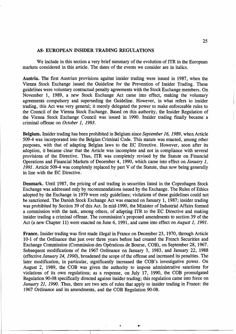
A8- EUROPEAN INSIDER TRADING REGULATIONS

We inelude in this section a very brief surnmary of the evolution of ITR in the European� markets considered in this article. The dates of the events we consider are in italics.�

Austria. The first Austrian provisions against insider trading were issued in 1987, when the� Vienna Stock Exchange issued the Guideline for the Prevention of Insider Trading. These� guidelines were voluntary contractual penalty agreements with the Stock Exchange members. On� November 1, 1989, a new Stock Exchange Act carne into effect, making the voluntary� agreements compulsory and superseding the Guideline. However, in what refers to insider� trading, this Act was very general; it merely delegated the power to make enforceable rules to� the Council of the Vienna Stock Exchange. Based on this authority, the Insider Regulation of� the Vienna Stock Exchange Council was issued in 1990. Insider trading finally became a� criminal offense on October 1, 1993.�

Belgium. Insider trading has been prohibited in Belgium since September 16, 1989, when Artiele� 509-4 was incorporated into the Belgian Criminal Codeo This statute was enacted, among other� purposes, with that of adapting Belgian laws to the EC Directive. However, soon after its� adoption, it became clear that the Artiele was incomplete and not in compliance with several� provisions of the Directive. Thus, ITR was completely revised by the Statute on Financial� Operations and Financial Markets of December 4, 1990, which carne into effect on January 1,� 1991. Artiele 509-4 was completely replaced by part V of the Statute, thus now being generally� in line with the EC Directive.�

Denmark. Until1987, the pricing of and trading in securities listed in the Copenhagen Stock� Exchange was addressed only by recornmendations issued by the Exchange. The Rules of Ethics� adopted by the Exchange in 1979 were only guidelines; violations of these guidelines could not� be sanctioned. The Danish Stock Exchange Act was enacted on January 1, 1987; insider trading� was prohibited by Section 39 of this Act. In mid-1990, the Minister of Industrial Affairs formed� a cornmission with the task, among others, of adapting ITR to the EC Directive and making� insider trading a criminal offense. The cornmission's proposed amendments to section 39 of the� Act (a new Chapter 11) were enacted on June 6, 1991, and carne into effect on August 1, 1991.�

France. Insider trading was first made illegal in France on December 23, 1970, tbrough Article� 10-1 of the Ordinance that just over tbree years before had created the French Securities and� Exchange Cornmission (Cornmission des Opérations de Bourse, COB), on September 28, 1967.� Subsequent modifications of the 1967 Ordinance on January 3, 1983, and January 22, 1988� (effective January 24, 1990), broadened the scope ofthe offense and increased its penalties. The� later modification, in particular, signiflcantly increased the COB's investigative power. On� August 2, 1989, the COB was given the authority to impose administrative sanctions for� violations of its own regulations; as a response, on July 17, 1990, the COB promulgated� Regulation 90-08 specifically directed against insider trading; this regulation carne into force on� January 21, 1990. Thus, there are two sets of rules that apply to insider trading in France: the� 1967 Ordinance and its amendments, and the COB Regulation 90-08.�

.----------------------.,.-----------------------------­

26

Germany. In November of 1970, the Voluntary Insider Trading Guidelines and the Broker and Investment Advisor Rules were put into effect; they were later revised in 1971, 1976, and 1988. The Guidelines were voluntary and adherence was based upon contracto Most corporations required senior management and potential insiders to enter into contracts with the corporation assenting adherence to these Guidelines and the Code of Procedure. Regulations that made insider trading a criminal offense were implemented on August 1, 1994.

Italy. The first Italian law specifically addressing insider trading (Law 153) was enacted on May 17, 1991, and carne into force on May 21, 1991. Until then, no regulation in Italian law prohibited insider trading, although attempts had been made to apply regulations conceived for other purposes to insider trading. Law 153 satisfies the requirements of the EC Directive.

Holland. Insider trading has been prohibited in Holland since February 16, 1989, day in which Article 336a of the Dutch Criminal Code carne into force. However, as early as 1973, the Committee on Corporate Law set up by Minister of Justice had already recommended penalties for insider trading. The Dutch criminal provisions were put into effect before the publication of the EC Directive; they satisfy the Directive fully, and, in sorne respects, they go even further.

Norway. The first Norwegian regulations on insider trading were contained in Act 61 of June 14, 1985 on Securities Trading, which carne into effect on October 15, 1985. This Act was later amended (adding sections 6a and 6b) by Act 75 of November 8, 1991. Sections 6a and 6b carne into effect on February 10, 1992, and other parts of section 6 on March 1, 1993.

Sweden. In the early 1970s, insiders in listed companies were required to disclose the holdings (and changes in holdings) in their companies, but the legislation contained no sanctions for insider offenses. In the mid-1980s specific criminal sanctions were introduced for insider trading offenses through the Securities Market Act (SFS 1985:571), which carne into effect on October 1, 1985. After a complete reevaluation of securities markets regulations, the Insider Act (SFS 1990: 1342) was adopted and carne into effect on February 1, 1991. This new act broadened the definition of insiders, extended the prohibition to all kinds of instruments in the securities markets, and increased the severity of the sanctions.

Switzerland. On November 16, 1981, in the case Sto loe Mineral v. BS/, the federal district court of the Southern District of New York subjected a Swiss bank to a significant daily fine for as long as it refused to reveal information to the SEC about the narne of a client for whom transactions had been made in the American stock market. This ruling provided incentives, already under way, to enact regulations against insider trading. On August 31, 1982, a Memorandum of Understanding (MOU) was signed between Switzerland and the US concerning collaboration in matters of mutual legal assistance. Convinced of the need for action the Swiss congress decided to focus on insider trading. A bill was approved on December 18, 1987, and a new MOU was signed with the US on November 17, 1987. Insider trading was finally prohibited in Switzerland on luly 1, 1988, day in which Artiele 161 of the Swiss Penal Code carne into effect. Under this Article, insider trading is a criminal offense.

27

REFERENCES�

Akgiray, Vedat (1989). "Conditionál Heteroskedasticity in Time Series of Stock Returns: Evidence and Forecasts." Journal of Business, 62, 55-80.

Black, Fisher (1976). "Studies of Stock Market Volatility Changes." Proceedings of the American Statistical Association, Business and Economics Studies Section, 177-81.

Bollerslev, Tim (1986). "Generalized Autoregressive Conditional Heteroskedasticity." Journal of Econometrics, 31, 307-327.

Bollerslev, Tim, Ray Chou, and Kenneth Kroner (1992). "ARCH Modelling in Finance. A Review of the Theory and Empirical Evidence." Journal of Econometrics, 52, 5-59.

Brown, Stephen, and Jerold Warner (1985). "Using Daily Stock Returns. The Case of Event Studies." Journal of Financial Economics, 14, 3-31.

Brudney, Victor (1979). "Insiders, Outsiders, and Informational Advantages Under the Federal Securities Laws." Harvard Law Review, 93, 322-376.

Cornell, Bradford, and Erik Sirri (1992). "The Reaction of Investors and Stock Prices to Insider Trading." Journal of Finance, 47, 1031-1059.

Corrado, Charles (1989). "A Nonparametric Test for Abnormal Security-Price Performance in Event Studies." Journal of Financial Economics, 23, 385-395.

Engle, Robert (1982). "Autoregressive Conditional Heteroskedasticity with Estimates of the Variance of U.K. Inflation." Econometrica, 50, 987-1008.

Engle, Robert, and Tim Bollerslev (1986). "Modelling the Persistence of Conditional Variances." Econometric Reviews, 5, 1-50.

Engle, Robert, David Lillien, and Russell Robbins (1987). "Estimating Time Varying Risk Premia in the Term Structure: The ARCH-M Model." Econometrica, 55, 391-407.

Estrada, Javier (1994). "Insider Trading: Regulation, Deregulation, and Taxation." Swiss Review of Business Law, 5/94, 209.

Estrada, Javier (1995). "Insider Trading: Regulation, Securities Markets, and Welfare Under Risk Aversion." Quarterly Review of Economics and Finance, jorthcoming.

Finnerty, Joseph (1976). "Insiders and Market Efficiency." Journal of Finance, 31, 1141-48.

28

Gaillard, Ernmanuel (1992). Insider Trading. The Laws o/Europe, the United States and Japan. Kiuwer Law and Taxation.

Jaffe, Jeffrey (1974). "The Effect of Regulation Changes on Insider Trading." Bell Joumal of Economics and Management Science, 5, 93-121.

Jarrell, Gregg, and Annete Poulsen (1989). "Stock Trading Before the Announcement ofTender Offers: Insider Trading or Market Anticipation?" Joumal ofLaw, Economics, and Organization, 5, 225-248.

John, Kose, and Larry Lang (1991). "Insider Trading Around Dividend Announcements: Theory and Evidence." Joumal of Finance, 46, 1361-1390.

Keown, Arthur, and John Pinkerton (1981). "Merger Announcements and Insider Trading Activity: An Empirical Investigation." Joumal of Finance, 36, 855-869.

Leland, Hayne (1992). "Insider Trading: Should It Be Prohibited?" Joumal of Political Economy, 100, 859-887.

Lo, Andrew, and Craig MacKinlay (1990). "An Econometric Analysis of Nonsynchronous Trading." Joumal of Econometrics, 45, 181.

Macey, Jonathan (1991). Insider Trading. Economics, Politics and Policy. American Enterprise Institute for Public Policy Research.

Mandelbrot, Benoit (1963). "The Variation of Certain Speculative Prices." Joumal of Business, 36, 394-419.

Manne, Henry (1966). Insider Trading and the Stock Market. The Free Press, New York.

Meulbroek, Lisa (1992). "An Empirical Analysis of Illegal Insider Trading." Joumal of Finance, 47, 1661-1699.

Nelson, Daniel (1991). "Conditional Heteroskedasticity in Asset Retums: A New Approach." Econometrica, 59, 347-370.

Scholes, Myron, and Joseph Williams (1987). "Estimating Betas From Nonsynchronous Data." Joumal of Financial Economics, 5, 309-327.

Seyhun, Nejat (1992). "The Effectiveness of the Insider-Trading Sanctions." Joumal of Law and Economics, 35, 149-182.

Standen, Daniel (1995). "Insider Trading Refonns Sweep Across Gennany: Bracing for the Cold Winds of Change." Harvard Intemational Law Joumal, 36, 177-206.