Facultad de Ciencias Económicas y Empresariales

Working Paper nº 23/12

Liquidity Commonalities in the Corporate CDS Market around the 2007-2012 Financial Crisis

Sergio Mayordomo University of Navarra

Juan Ignacio Peña Universidad Carlos III de Madrid

María Rodríguez-Moreno European Central Bank

Liquidity Commonalities in the Corporate CDS Market around the 2007-2012 Financial Crisis Sergio Mayordomo, Juan Ignacio Peña, María Rodríguez-Moreno Working Paper No.23/12 December 2012

ABSTRACT This study presents robust empirical evidence suggesting the existence of significant liquidity commonalities in the corporate Credit Default Swap (CDS) market. Using daily data for 438 firms from 25 countries in the period 2005-2012 we find that these commonalities vary over time, being stronger in periods in which the global, counterparty, and funding liquidity risks increase. However, commonalities do not depend on firm’s characteristics. The level of the liquidity commonalities differs across economic areas being on average stronger in the European Monetary Union. The effect of market liquidity is stronger than the effect of industry specific liquidity in most industries excluding the banking sector. We document the existence of asymmetries in commonalities around financial distress episodes such that the effect of market liquidity is stronger when the CDS market price increases. The results are not driven by the CDS data imputation method or by the liquidity of firms with high credit risk and are robust to alternative liquidity measures. Sergio Mayordomo School of Economics and Business Administration University of Navarra smayordomo@unav.es Juan Ignacio Peña Department of Business Administration Universidad Carlos III de Madrid ypenya@eco.uc3m.es María Rodríguez-Moreno European Central Bank maria.rodriguez_moreno@ecb.int

1

Liquidity Commonalities in the Corporate CDS Market around the 2007-2012 Financial Crisis

Sergio Mayordomoa, Juan Ignacio Peñab, María Rodríguez-Morenoc

This version: 16/10/2012

First version: 07/11/2011 a University of Navarra, School of Economics and Business Administration; Edificio Amigos; 31009

Pamplona, Spain; smayordomo@unav.es b Department of Business Administration; Universidad Carlos III de Madrid C/ Madrid 126, 28903

Getafe (Madrid, Spain); ypenya@eco.uc3m.es c European Central Bank; Neue Mainzer Strasse 66, 60311Frankfurt am Main (Germany);

maria.rodriguez_moreno@ecb.int _____________________________________________________________________

Abstract

This study presents robust empirical evidence suggesting the existence of significant liquidity commonalities in the corporate Credit Default Swap (CDS) market. Using daily data for 438 firms from 25 countries in the period 2005-2012 we find that these commonalities vary over time, being stronger in periods in which the global, counterparty, and funding liquidity risks increase. However, commonalities do not depend on firm’s characteristics. The level of the liquidity commonalities differs across economic areas being on average stronger in the European Monetary Union. The effect of market liquidity is stronger than the effect of industry specific liquidity in most industries excluding the banking sector. We document the existence of asymmetries in commonalities around financial distress episodes such that the effect of market liquidity is stronger when the CDS market price increases. The results are not driven by the CDS data imputation method or by the liquidity of firms with high credit risk and are robust to alternative liquidity measures.

Keywords: Credit Default Swap, Liquidity Commonalities, Global Risk, Funding Liquidity Risk, Counterparty Risk JEL codes: G12, G15

______________________________________________________________________

2

1. Introduction

One of the key issues highlighted by the ongoing financial crisis is the role of the shortage of

liquidity in financial markets. In this period we have witnessed severe episodes of liquidity

shortage in many markets being this shortage especially noticeable in the Credit Default

Swap (CDS) market because of the uncertainty about the net amount, the structure, and the

counterparty risk of such exposures. As a consequence, many firms have had difficulties to

timely manage their credit risk exposures. This situation posed important challenges at the

individual level but also from a global stability perspective. These facts point out the

importance of considering the extent to which the shortage of liquidity has spread over the

different contracts traded in the CDS market, and the factors that affect such scarcity.

This paper focuses on factors that may affect this shortage in market liquidity, and

specifically the extent to which liquidity commonalities in the CDS market are of material

importance in this regard. Liquidity commonalities can be defined as the co-movement of

individual liquidity measures with market- and industry-wide liquidity. The objective of this

paper is to provide new evidence on the co-movement in liquidity for the CDS market, which

was firstly documented by Pu (2009), from a threefold perspective: first, the analysis of the

time-varying behavior of the commonalities putting special emphasis on the financial crisis

events; secondly, the use of different economic areas and industries for the analysis of such

commonalities; and, thirdly the analysis of the factors influencing this co-movement at both

aggregate and firm levels.

The typology of the participants in the CDS market, the high degree of concentration, and the

role of credit derivatives during the financial crisis affecting both the financial sector and real

economy make the analysis of the existence and the behavior of liquidity commonalities in

the CDS market a topic of special relevance for regulators, risk managers, and investors. The

fact that the main participants in the CDS market are systemically important financial

3

institutions (SIFIs) facilitates that any shock affecting credit derivatives could revert directly

on these institutions and could have implications in terms of financial stability. In this line,

Rodriguez-Moreno et al. (2012) show that the holdings of credit derivatives by U.S. banks

affected their contributions to systemic risk, such that these derivatives behaved as shock

absorbers before the financial crisis but changed their role to shock issuers during the crisis. It

is worth mentioning that the liquidity risk derived from the typology of the banks

participating in the CDS market could be exacerbated by the high degree of concentration of

the market activity in the hands of a few SIFIs acting as market participants.1 This high

degree of market concentration may have implications in terms of the impact of large shocks

on market liquidity. In fact, Mayordomo and Peña (2012) show that liquidity commonalities

have significant effects on the pricing of the CDS of European non-financial firms and on the

co-movements among CDS prices during the recent financial crisis.

The analysis of the determinants of the commonalities in liquidity is also certainly a timely

topic because, as remarked by Dewatripont et al. (2010), developing a better understanding of

what drives illiquidity at the individual and aggregate levels should stand high on the agenda

of economists and policy makers alike.

We contribute with several findings to the empirical literature on liquidity commonalities.

We document the existence of significant co-movements between single-name CDS liquidity

and market-wide liquidity. Market commonalities are stronger than industry commonalities in

most industries, with the exception of the banking sector. The liquidity commonalities are

1 According to a survey of U.S. firms by Fitch (2009), 96% of credit derivative exposures at the end of the first

quarter of 2009 were concentrated in 5 firms (JPMorgan, Goldman Sachs, Citigroup, Morgan Stanley, and Bank

of America). According to the Bank of International Settlements reports, globally the ten largest dealers account

for 90% of trading volume by gross notional amount, 30% of the global activity is generated by just one bank

(JP Morgan) and in the US five banks account for more than 90% of the gross notional.

4

still present when we analyze separately the CDSs of companies located in different

economic areas, but the degree of commonality differs across them. Moreover, the liquidity

commonalities are time-varying and increase in times of financial distress characterized by

high counterparty, global, and funding liquidity risks but they do not depend on firms’

specific characteristics. In this line, we find that the Lehman Brothers collapse and the Greek

bailout requests triggered a significant increase in commonalities. In fact, the results suggest

the existence of asymmetries in commonalities around these episodes of financial distress,

such that the effect on market liquidity is stronger when the CDS market price increases.

Finally, we find that liquidity commonalities provide additional information relative to the

three aforementioned aggregate risks around these periods. All these results are robust to

alternative liquidity measures and are not driven by the CDS data imputation method or by

the firms with the highest CDS prices.

The rest of this article is organized as follows. Section 2 presents a literature review. In

Section 3 we describe the liquidity measures and the methodology. Section 4 describes the

data. Section 5 reports the empirical findings regarding the existence of liquidity

commonalities. Section 6 reports the results of the determinants of these commonalities. In

Section 7 we present some robustness tests, and we conclude in Section 8.

2. Literature Review

The Acharya and Pedersen’s (2005) liquidity-adjusted Capital Asset Pricing Model (CAPM)

yields three effects, besides the covariance between the asset’s return and the market return,

that provide a characterization of the liquidity risk of a security. The first of these effects on

expected returns is due to the covariance between a security’s expected return and the market

liquidity. The second effect on expected returns is due to the co-variation between a

security’s illiquidity and the market return. The third of these effects is that the return

5

increases with the covariance between the asset’s illiquidity and the market illiquidity given

that investors want to be compensated for holding a security that becomes illiquid when the

market in general becomes illiquid. This last component is the common factor in liquidity or

liquidity commonalities documented in the stock market by Chordia et al. (2000), Hasbrouck

and Seppi (2001), and Huberman and Halka (2001).

Our paper belongs to the growing literature on liquidity risk and follows the Chordia, et al.’s

(2000) methodology to study the time-varying nature and the determinants of the liquidity

commonalities in the CDS market. Thus, the other two liquidity risk components and the

effect of the liquidity commonalities on the CDS premium are beyond the scope of this paper.

Several methodologies have been used to study the existence of liquidity commonalities.2 A

detailed comparison of the different estimators can be found in Anderson et al. (2010). These

authors distinguish two classes of methodologies for the estimation of systematic liquidity:

(1) weighted average estimators based on concurrent liquidity shocks (the one employed in

our study), and (2) principal component estimators based on both concurrent and past

liquidity shocks. Their results show that the two types of estimators are largely equivalent

because the simpler estimators give, in most cases, similar results to the complex estimators

under different evaluation criteria and liquidity measures. Following Chordia et al. (2000),

we use cross-sectional equally weighted averages to construct the market liquidity measure

employed for the estimation of liquidity commonalities.

2 There is a wide array of variables to measure liquidity but one of the most common liquidity measures

employed in the fixed-income and the CDS literature is the bid–ask spread. In fact, Fleming (2003) finds that

the bid–ask spread is the best measure of liquidity in the bond market. For this reason, the primary liquidity

measure employed in our baseline analysis focuses on the bid–ask spread.

6

The existence of liquidity commonalities has been documented for many assets

independently of the dimension of liquidity and the geographical area analyzed. The foremost

market in which liquidity commonalities have been documented is the stock market (see

Chordia et al., 2000; Hasbrouck and Seppi, 2001; Huberman and Halka, 2001; Brockman and

Chung, 2002; Domowitz et al., 2005; Kamara et al., 2008; Kempf and Mayston, 2008; or

Korajczyk and Sadka, 2008; among others). Liquidity commonalities across different stock

markets located in different countries have also been documented by previous literature (see

for instance Brockman et al., 2009; Karolyi et al., 2009; or Zhang et al., 2009).

There are also several examples of analysis of liquidity commonalities for other markets in

addition to the stock market. Thus, Chordia et al. (2005) and Goyenko (2009) document the

commonality in liquidity for stocks and bonds in the United States (U.S.) market. Liquidity

commonalities are also documented by Marshall et al. (2010) in the commodities markets and

by Cao and Wei (2010) in the options market. Cao and Wei (2010) find strong commonalities

in the option market but these commonalities are lower than those of the stock market.

However in the case of the CDS market this topic has been barely addressed. Pu’s (2009) is

the first paper that considers explicitly the commonalities in the CDS market. This author

finds a strong commonality across all liquidity measures in the CDS market and also in the

bond market using monthly data from 2002 to 2005 for a sample of non-financial U.S. firms.

The method employed by Pu (2009) to extract the common factors from each liquidity

measure is an asymptotic principal component analysis.

Liquidity commonalities in the CDS market are also treated indirectly in other papers such as

Bongaerts et al. (2011) and Jacoby et al. (2009). Bongaerts et al. (2011) derive and estimate a

model for the pricing of liquidity in the CDS market. Among the variables considered is the

level of liquidity commonalities that is obtained from a principal component analysis across

CDS portfolios. The first factor of this analysis explains 16.6% of the liquidity variation.

7

Jacoby et al. (2009) analyze the existence of liquidity spill-over shocks across the CDS,

corporate bond, and equity markets and find a dominant first principal component in the CDS

market for the CDS liquidity measures considered. Other papers that study the determinants

of bid-ask spread use market liquidity as an additional driver of individual CDSs’ liquidity

(e.g. Meng and ap Gwilym, 2008; or Tang and Yan, 2008).

The aim of this paper is not to study the effect the determinants of bid-ask spreads but to

estimate the effect of market liquidity on the individual CDS liquidity according to the

standard methodology of liquidity commonalities. We share some of the objectives pursued

by Pu (2009) but in contrast to her analysis, our study is carried out using daily data that

covers the recent financial crisis and documents both the time varying behavior of liquidity

commonalities and their determinants during this crisis. Additionally, our paper exploits a

much more extensive database which allows us to deal explicitly with the differences in terms

of commonalities of the different economic areas besides the US, and also to include firms

from all sectors.

Besides documenting the existence of commonalities in liquidity, other stream of the

literature analyzes the drivers of such commonalities. In one of these papers, Coughenour and

Saad (2004) find that the individual stock liquidity co-varies with specialist portfolio liquidity

given that the specialist firms that participate in the stock market provide liquidity for more

than one common stock. This co-variation increases with the risk of providing liquidity. The

role of capital constraints on stock market liquidity commonality is documented by

Comerton-Forde et al. (2010) and Brunnermeier and Pedersen (2009).

Brunnermeier and Pedersen (2009) find that the effect of funding constraints is particularly

important during market downturns. Situations of market stress have also been found to affect

liquidity commonalities. Thus, Kempf and Mayston (2005) find that the commonality in the

stock market is much stronger in falling markets than in rising markets. Brockman and Chung

8

(2008) find that commonality in order-driven markets (in their case the Hong Kong Stock

Exchange) increases during periods of market stress.

As Anderson et al. (2010) suggest, the degree and variation of commonality in liquidity could

also be affected by the concentration of market makers and the type of trading. In fact,

Kamara et al. (2008) find that increases in institutional ownership are associated with

increases in stocks’ sensitivity to systematic liquidity shocks. These authors show that during

the period 1963–2005 commonality in liquidity increased significantly for large-cap stocks,

in which institutional investing and index trading were more concentrated, but declined

significantly for small-cap stocks.

In the best of our knowledge ours is the first paper documenting the determinants of liquidity

commonalities in the CDS market at both aggregate and firm levels. We find that the level of

liquidity commonalities is related to a large extent to global risk factors and therefore this

level seems to be a potentially useful instrument to monitor global risk.

3. Liquidity Measures and Methodology

3.1. Liquidity Measures

Our baseline liquidity measure is the relative quoted spread (RQS), for a given firm j at time t

defined as:

푅푄푆 , =퐴푠푘 , −퐵푖푑 ,

(퐴푠푘 , + 퐵푖푑 , )2

(1)

This measure has been widely employed in the previous literature and avoids any bias in the

results due to the dependence on the level of the CDS premium or the degree of risk as could

be the case when one uses the bid–ask CDS spread in absolute terms. However, to ensure that

the results do not depend solely on the liquidity specification we use other liquidity measures:

- The absolute bid–ask spread (AQS) defined as the difference between CDS ask and

bid prices without rescaling by the mid spread as in the RQS (equation (1)).

9

- Number of contributed quotes in a given day, which represents the depth of the

consortium liquidity.

- Number of contributors: the number of contributors providing quotes, which

represents the breadth of the consortium coverage.

- The gross and net weekly traded notional CDS amount outstanding and the number of

contracts outstanding.3

3.2. Estimation Methodology of Liquidity Commonalities

3.2.1. Baseline market model

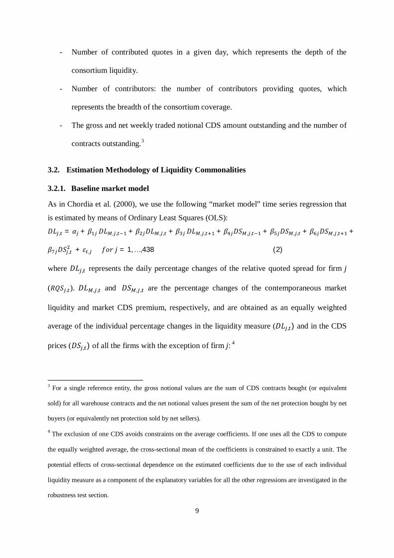
As in Chordia et al. (2000), we use the following “market model” time series regression that

is estimated by means of Ordinary Least Squares (OLS):

퐷퐿 , = 훼 + 훽 퐷퐿 , , + 훽 퐷퐿 , , + 훽 퐷퐿 , , + 훽 퐷푆 , , + 훽 퐷푆 , , + 훽 퐷푆 , , +

훽 퐷푆 , + 휀 , 푓표푟푗 = 1, … ,438(2)

where 퐷퐿 , represents the daily percentage changes of the relative quoted spread for firm j

(푅푄푆 , ). 퐷퐿 , , and 퐷푆 , , are the percentage changes of the contemporaneous market

liquidity and market CDS premium, respectively, and are obtained as an equally weighted

average of the individual percentage changes in the liquidity measure (퐷퐿 , ) and in the CDS

prices (퐷푆 , ) of all the firms with the exception of firm j: 4

3 For a single reference entity, the gross notional values are the sum of CDS contracts bought (or equivalent

sold) for all warehouse contracts and the net notional values present the sum of the net protection bought by net

buyers (or equivalently net protection sold by net sellers).

4 The exclusion of one CDS avoids constraints on the average coefficients. If one uses all the CDS to compute

the equally weighted average, the cross-sectional mean of the coefficients is constrained to exactly a unit. The

potential effects of cross-sectional dependence on the estimated coefficients due to the use of each individual

liquidity measure as a component of the explanatory variables for all the other regressions are investigated in the

robustness test section.

10

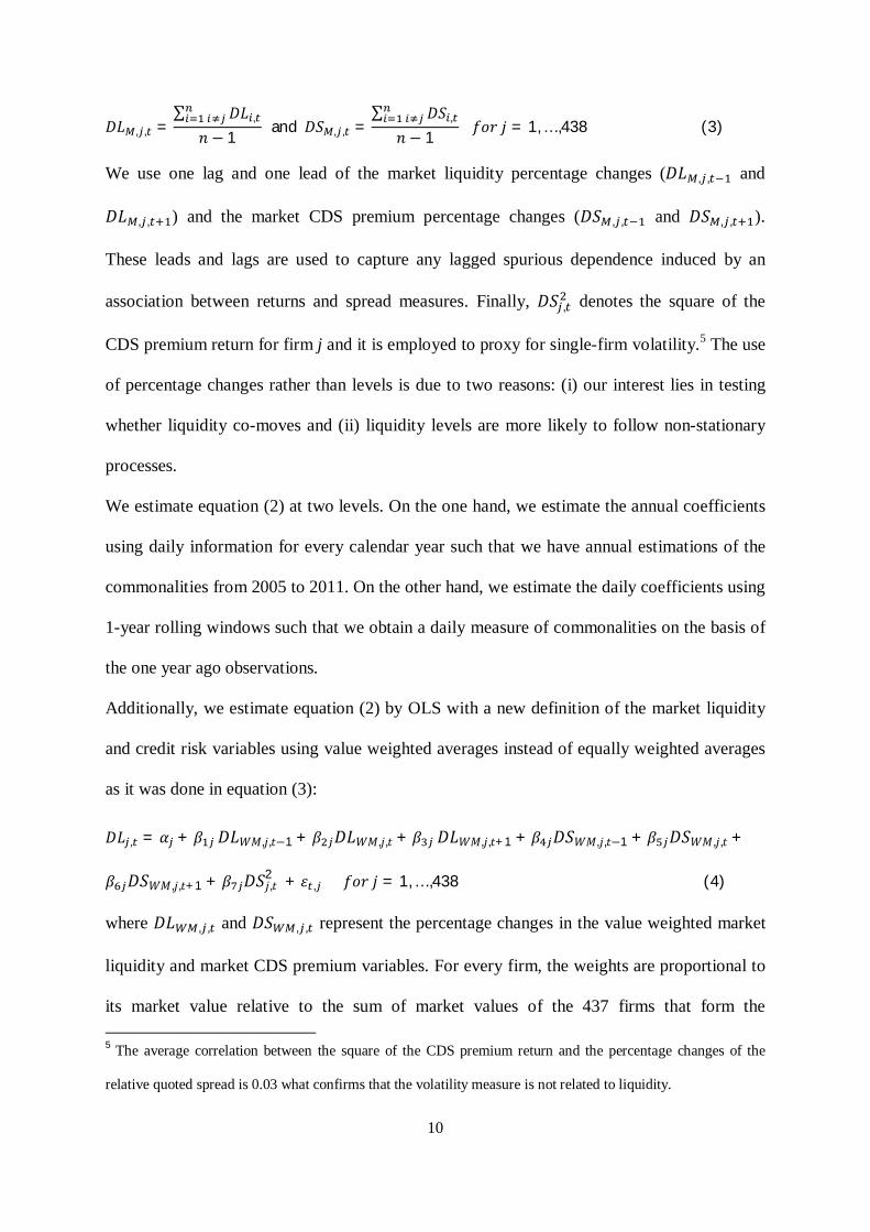
퐷퐿 , , =∑ 퐷퐿 ,

푛 − 1and퐷푆 , , =

∑ 퐷푆 ,

푛 − 1푓표푟푗 = 1, … ,438(3)

We use one lag and one lead of the market liquidity percentage changes (퐷퐿 , , and

퐷퐿 , , ) and the market CDS premium percentage changes (퐷푆 , , and 퐷푆 , , ).

These leads and lags are used to capture any lagged spurious dependence induced by an

association between returns and spread measures. Finally, 퐷푆 , denotes the square of the

CDS premium return for firm j and it is employed to proxy for single-firm volatility.5 The use

of percentage changes rather than levels is due to two reasons: (i) our interest lies in testing

whether liquidity co-moves and (ii) liquidity levels are more likely to follow non-stationary

processes.

We estimate equation (2) at two levels. On the one hand, we estimate the annual coefficients

using daily information for every calendar year such that we have annual estimations of the

commonalities from 2005 to 2011. On the other hand, we estimate the daily coefficients using

1-year rolling windows such that we obtain a daily measure of commonalities on the basis of

the one year ago observations.

Additionally, we estimate equation (2) by OLS with a new definition of the market liquidity

and credit risk variables using value weighted averages instead of equally weighted averages

as it was done in equation (3):

퐷퐿 , = 훼 + 훽 퐷퐿푊푀,푗,푡−1 + 훽 퐷퐿푊푀,푗,푡 + 훽 퐷퐿푊푀,푗,푡+1 + 훽 퐷푆푊푀,푗,푡−1 + 훽 퐷푆푊푀,푗,푡 +

훽 퐷푆푊푀,푗,푡+1 + 훽 퐷푆푗,푡2 + 휀 , 푓표푟푗 = 1, … ,438(4)

where 퐷퐿 , , and 퐷푆 , , represent the percentage changes in the value weighted market

liquidity and market CDS premium variables. For every firm, the weights are proportional to

its market value relative to the sum of market values of the 437 firms that form the 5 The average correlation between the square of the CDS premium return and the percentage changes of the

relative quoted spread is 0.03 what confirms that the volatility measure is not related to liquidity.

11

considered market. As we are using firms from different countries the market values are

uniformly defined in U.S. Dollars.6

The 438 reference entities employed in this paper correspond to 25 countries that we assign

to 5 economic areas. Due to their heterogeneity, we alternatively construct the market

liquidity and market CDS premium measures at economic area level (i.e., using only the

firms that belong to the same economic area of firm j in equation (3)). Then, we use these

new measures as explanatory variables to estimate the liquidity commonalities by OLS

according to the specification of equation (5).

퐷퐿 , = 훼 + 훽 퐷퐿푀,푖,푗,푡−1 + 훽 퐷퐿푀,푖,푗,푡 + 훽 퐷퐿푀,푖,푗,푡+1 + 훽 퐷푆푀,푖,푗,푡−1 + 훽 퐷푆푀,푖,푗,푡 +

훽 퐷푆푀,푖,푗,푡+1 + 훽 퐷푆푗,푡2 + 휀 , 푓표푟푗 = 1, … ,438andi = 1, … ,5(5)

where 퐷퐿 , , , and 퐷푆 , , , represent the percentage changes in the equally weighted market

liquidity and market returns variables of economic area i.

3.2.2. Market model with asymmetries in liquidity commonalities

We next split up the contemporaneous effect of the market liquidity variable into two effects

depending on whether the market CDS returns have a positive or negative sign. For such aim,

we use two interaction variables obtained as the product of the percentage changes in market

liquidity and two different dummy variables: (i) a dummy 푑 that takes value one when

the market CDS premium is going up at a given date; and (ii) a dummy 푑 that takes

value one when the market CDS premium is going down. We use the same methodology as

in equation (2) but excluding the lagged and lead values of the changes in market liquidity

from the estimation such that the new equation is defined as follows:

6 Market values converted to the common currency are directly downloaded from Datastream. This database

uses the corresponding daily exchange rate to convert the market value in the domestic currency to US Dollars.

12

퐷퐿 , = 훼 + 훽 푑 퐷퐿 , , + 훽 푑 퐷퐿 , , + 훽 퐷푆 , , + 훽 퐷푆 , , + 훽 퐷푆 , , +

훽 퐷푆 , + 휀 , 푓표푟푗 = 1, … ,438(6)

3.2.3 Two variations of the standard market model

We first examine in more detail the effect of liquidity commonalities using both market and

industry equally weighted liquidity measures. We add lagged, contemporaneous, and leading

industry liquidity variables to equation (2):

퐷퐿 , = 훼 + 훽 퐷퐿 , , + 훽 퐷퐿 , , + 훽 퐷퐿 , , + 훽 퐷푆 , , + 훽 퐷푆 , , + 훽 퐷푆 , , +

훽 퐷푆 , + 훽 퐷퐿 , , + 훽 퐷퐿 , , + 훽 퐷퐿 , , + 휀 , 푓표푟푗 = 1, … ,438(7)

where 퐷퐿 , , is the percentage change in the industry liquidity, obtained using only the firms

that belong to the same industry that firm j in equation (3). We consider 28 out of 41

industries distinguished by the Industry Classification Benchmark (ICB), which is available

from Datastream.7

We then test the hypothesis that the reference entities with the highest credit risk could be the

ones causing the commonality effect. For this reason, we add to the explanatory variable

group collected in equation (2) the percentage changes of the contemporaneous (퐷퐿 , , ),

lagged (퐷퐿 , , ), and leading (퐷퐿 , , ) high credit risk firms’ liquidity measure that is

constructed using only the firms that belong to the top quartile according to their level of

CDS prices in equation (3):8

퐷퐿 , = 훼 + 훽 퐷퐿 , , + 훽 퐷퐿 , , + 훽 퐷퐿 , , + 훽 퐷푆 , , + 훽 퐷푆 , , + 훽 퐷푆 , , +

훽 퐷푆 , + 훽 퐷퐿 , , + 훽 퐷퐿 , , + 훽 퐷퐿 , , + 휀 , 푓표푟푗 = 1, … ,438(8)

7 No information on CDS is available for the firms of the remaining 13 sectors in the ICB classification system.

8 The classification of a given firm among the firms in the top quartile according to the CDS premia is

performed on an annual basis. Alternatively we could use credit ratings instead of CDS premia. Both measures

should give an equivalent stratification. Nevertheless, we use CDS prices because according to previous

literature (see Hull et al., 2004, among others), the CDS premia seem to anticipate the rating announcements.

13

3.3. Estimation Methodology of the Determinants of Liquidity Commonalities

We study the determinants of liquidity commonalties at aggregate and firm levels. To

proceed with the former analysis we first estimate the individual monthly liquidity

commonalities using daily information for every calendar month where the market model is a

variation of equation (2) in which we do not include the leads and lags of any variable:

퐷퐿 , = 훼 + 훽 , 퐷퐿 , , + 훽 , 퐷푆 , , + 훽 , 퐷푆 , + 휀 , forj = 1, … ,438(9)

We next construct the monthly aggregate beta as the median of the firm’s betas referring to

the contemporaneous market liquidity (훽 , in equation (9)). Finally, we conduct the

following analysis:

푀푒푑푖푎푛(훽 ) = 휂 + 휂 푅푖푠푘퐹푎푐푡표푟 + 휀 (10)

in which we regress the aggregate betas for every month m on the monthly averages of three

risk factors: global risk, global liquidity/ funding costs, and counterparty risk in the CDS

market. We use a robust to heteroscedasticy OLS methodology to estimate the effect of the

above variables.

The analysis of the determinants of the market liquidity on individual liquidity is carried out

on the basis of the daily liquidity commonalities estimated in equation (2) using 1-year

rolling windows. Concretely, we use the sum of the betas for the lagged, contemporaneous

and lead market liquidity measures as the dependent variable. As the liquidity commonalities

are based on overlapping information, we run a Fama-MacBeth cross-sectional regression for

every day in the sample to avoid time series dependencies and to exploit the cross-sectional

dimension. The standard errors are corrected for autocorrelation using the Newey-West

methodology.9

9 The number of lags employed in the Newey-West regressions must grow with the sample size to ensure

consistency when the moment conditions are dependent. We use a lag length determined by the widely

employed method of the number of observations raised to the power of 1/3 that is equal to 12 lags.

14

푆푢푚퐵푒푡푎푠 , = 훿 + 훿 퐹푖푟푚퐼푛푓표 , + 훿 퐶표푢푛푡푟푦퐼푛푓표 , + 휀 푤ℎ푒푟푒푡 = 1, … , 1625(11)

Among the determinants of the co-variation between the CDS and market illiquidity

measures we use firm and country specific variables. Among the former variables, we use

proxies for the firm size, leverage, level of credit risk, and firm shares’ squared returns

(volatility). Among the variables referred to the country of origin of the firm, we use proxies

for the volatility of the stock indexes and 3-month interbank interest rate.

4. Data

The data consist of daily 5-year CDS information for 438 listed firms from 25 countries and

span from 1 January 2005 to 31 March 2012.10 Due to the variety of countries and to ensure a

minimum number of firms in subsequent analysis we group them into 5 economic areas: the

U.S. (236 firms), the European Monetary Union (E.M.U., 108 firms), the United Kingdom

(U.K., 41 firms), Japan (15 firms), and Others (28 firms).

CDS information is obtained from Credit Market Analysis (CMA), an independent CDS data

provider that is part of the Chicago Mercantile Exchange. CMA sources its CDS data from a

consortium consisting of around 40 members of the buy-side community (hedge funds, asset

managers, and major investment banks) who are active participants in the CDS market. CMA

is found to be one of the more reliable CDS data sources by Mayordomo et al. (2010).

The information reported by CMA includes: (i) bid/mid/ask CDS premia for the 0.5 to 10

year maturities; (ii) an observed/derived indicator, which indicates whether the published

10 The sample does not include sovereign or unlisted reference entities. The use of the 5-year maturity CDS

contracts is due to the higher liquidity in these contracts. The reference entities belong to the following countries

(the number of firms in each country in brackets): the United States (236), the United Kingdom (41), France

(35), Germany (24), Japan (15), Canada (11), Italy (9), the Netherlands (9), Switzerland (7), Australia (6),

Finland (6), Spain (6), Sweden (6), Hong Kong (5), South Korea (4), Belgium (3), Malaysia (3), Portugal (3),

Ireland (2), Singapore (2), Austria (1), Denmark (1), Greece (1), New Zealand (1), and Norway (1).

15

level was observed in the market or implied through a model using recently observed

quotes;11 (iii) the number of contributors, which is the number of contributors providing

quotes; (iv) contributed quotes, which reports the number of contributed quotes on a given

day. The number of contributors and quotes is only available from June 2008. The nature of

the CMA data supposes an advantage for the use of the bid–ask spread as a measure of

liquidity, in addition to the other measures employed in the robustness test, because of the use

of information from the buy–sell sides.

The information for the gross and net notional CDS amount and the number of contracts

outstanding for each reference firm is obtained from the Depository Trust and Clearing

Corporation’s (DTCC). These data are only available for 399 of the 438 firms since

November 2008 and with a weekly frequency.

Next, we briefly describe the information employed to construct the remaining variables and

their sources. Information referring to global risk, which is proxied by the implied volatility

index (VIX), is obtained from Reuters.12 Due to the difficulty in obtaining data on

institutional-level funding constraints, we proxy the funding costs by means of the difference

between the 90-day U.S. AA-rated commercial paper interest rates for the financial

companies and the 90-day U.S. T-bill which should be a proxy for the funding cost faced by

AAA-rated financial investors. Both rates jointly with the 3-month interbank rate and the

country stock indexes are obtained from Datastream. As in Arce et al. (2012), we compute

the proxy for counterparty risk by means of the first principal component obtained from the

CDS premium of the main banks acting as dealers in the market. The information on the

11 CMA considers a CDS price as observed when they receive three different prices from at least two members

of its consortium. The CDS prices that do not fulfill this principle become derived prices.

12 According to Lustig et al. (2011) “the VIX seems like a good proxy for the global risk factor. The VIX is

highly correlated with similar volatility indices abroad”.

16

banks CDSs is obtained from CMA. The first principal component series should reflect the

common default probability that is an aggregate measure of counterparty risk.13 The

information on the firms’ stock prices, market capitalization, total debt and total assets is

obtained from Datastream.

Table 1 summarizes the most salient features of the descriptive statistics for related

information to the sample of CDS contracts. For the sake of brevity we focus on the annual

cross-sectional average of the mean, median and standard deviation (SD) from 2005 to 2011.

We also provide information about 2012 which refers to the first quarter of that year. Looking

at the CDS premium levels, we observe a gradual increase in the levels and their volatilities

from 2005 to 2009 and this behavior is common in both the total sample and in the economic

areas. In 2010 CDS prices perform on average a generalized drop. Average CDS prices

increase again in all economic areas apart from the U.S. in 2011 as a consequence of the

deterioration of the economic situation worldwide and especially in Europe.

Focusing on the bid-ask spreads, measured in basis points, their behavior is in line with the

CDS premium levels. Looking at the relative bid-ask spread, measured in percentage over

average price, we observe a gradual decrease in levels and volatilities from 2005 to 2011. It

implies that the liquidity in the CDS market tends to increase and its volatility to decrease

what is consistent with the market growing in size over time. Table 1 also contains the

squared of the CDS returns, which is used as a proxy of the individual volatility. We observe

that the higher average volatility is achieved in 2007 and 2008.

< Insert Table 1 here >

Regarding additional properties of the daily percentage changes of the relative bid-ask

spreads (퐷퐿 , ) employed in equation (2), this variable is equal to zero (no changes in the 13 We use the 14 main banks acting as dealers in the CDS market. The first PC for the series of CDS prices of

the previous dealers explains 90% of the total variance.

17

level of liquidity) for around 10% of the total number of observations. This occurs mainly at

the beginning of the sample coinciding with the early stages of the CDS market. This figure

supports the idea that results are not driven by the level of persistence in 퐷퐿 , . In fact, the

average autocorrelation of 퐷퐿 , is around -0.3 which suggests that autocorrelation is hardly a

relevant issue in our analysis.

5. Empirical Findings

5.1. Basic Empirical Evidence

We first test the co-variation between single-name CDS liquidity and CDS market-wide

liquidity per calendar year. Table 2 reports the results for the estimation of equation (2)

showing the cross-sectional averages of the slopes of the contemporaneous, lagged, and

leading market liquidity measures and the t-statistics over the 438 firms in our sample.14 The

table also includes the proportion of individual positive slopes and the proportion of

individual positive and significant (critical value 5%) coefficients. Finally, we report the

“sum” and “median”, which refer to the cross-sectional average and median of the sum of the

contemporaneous, lead, and lag betas, respectively. The coefficients are estimated year by

year from 2005 to 2011.15

The results show a positive and significant contemporaneous effect of the CDS market

liquidity variables on the individual liquidity measure, while the magnitude of the lagged and

leading coefficients is much lower and the number of significant coefficients only exceeds

14 Given that the individual disturbances in equation (2) are probably not normally distributed it is safer to

concentrate on the average cross-sectional results, the distribution of which is probably close to Gaussian under

some mild conditions.

15 We do not estimate the commonalities in liquidity for 2012 because we only have information for the first

quarter. However, we use the information of year 2012 in the later rolling windows estimation.

18

11% in 2010.16 The contemporaneous effect reaches its maximum values in 2007 and 2008

(0.82 and 0.86, respectively), both of them being highly significant. High significant values

are also found in 2010 and 2011 (0.78 and 0.79, respectively). On the other hand, the

minimum effect of the liquidity commonality occurs in 2005 (0.57) and 2006 (0.59).

On the basis of the sum of the three coefficients we find a positive and significant effect of

the CDS market liquidity on the individual liquidity measures over the eight years of the

sample. The median follows the same trend but the estimated levels are lower. The

explanatory power as measured by the R-squared is not very high, ranging from 4% in 2005

to 9% in 2010, but it is in line with other papers using the same methodology, such as

Chordia et al.’s (2000) analysis of the stock market commonalities. This fact suggests that

there are additional explanatory variables that this methodology is not identifying. An

interesting result is the trend observed in the liquidity commonalities which seem to evolve

over time according to the economic conditions. It suggests that liquidity commonalities

could be state-dependent as it is documented in Figure 1, which contains the cross-sectional

median of the sum of the contemporaneous, lead and lag daily coefficients using 1-year

rolling windows. Note that in the subsequent analysis we use the median to avoid any

potential extreme betas, although the correlation between the median and average betas

obtained in the baseline analysis is equal to 0.95.

< Insert Table 2 here >

Panel A of Figure 1 shows the median of the sum of liquidity commonalities from 2006 to

2012 obtained using the baseline methodology (equation (2)) and an alternative methodology

16 In some years such as 2005, 2006, and 2009 only 19, 14, and 28% of contemporaneous coefficients are

positive and significant, respectively. The maximum level of significance is achieved in 2008 (70%).

Nevertheless, this significance is not the one that determines the level of significance of liquidity commonalities

but the one referred to the aggregate (“Sum”) effect whose t-statistic is shown at the bottom of this Table 2.

19

in which market measures are constructed by means of value weighted averages by firm

capitalization (equation (4)). The first comment that applies is that both methods for

computing the market measures give similar trends given that the correlation between the two

measures is 0.94. The baseline methodology gives systematically stronger liquidity

commonalities before January 2008. After this date, the commonalities are larger under the

equally weighted specification but the differences are smaller than before January 2008. After

the Greek’s bailout requests, both methodologies provide very similar levels. A potential

explanation is that the liquidity of some large firms is not representative of the market

liquidity, especially before the main episodes of high risk, and so the co-variation of other

CDS contracts with the new market liquidity measure decreases.

Looking at the baseline specification we observe that the lowest levels of liquidity

commonalities occur during year 2006, which is a tranquil period. During the whole year

2007 there is a monotonic increasing trend. The high liquidity commonalities reached by the

end of 2007 persist until summer 2009 when there is a decrease that persists until the end of

the year. The levels of commonalities remain relatively constant until March 2010. From this

date commonalities exhibit a remarkable increase that reaches its maximum value around

May 2010, coinciding with the Greek rescue, and remains high until March 2011 when there

is a significant drop. A new increase is observed by June-July 2011 coinciding with the

European Council of 21st July in which there was a failure to arrive at a clearly articulated

and adequately funded agreement to guarantee the viability of Greece’s public finances.

Liquidity commonalities remain around this level until the end of the sample.

In view of the pattern of the commonalities in liquidity, we next study whether there are

significant changes around two relevant events related to the so-called subprime crisis

(Lehman Brothers’ collapse on September 15th, 2008) and sovereign debt crisis (Greek’s

bailout requests on April 23rd, 2010); on the basis of the liquidity commonalities obtained in

20

the baseline analysis (equation (2)). For such aim, we carry out a mean test comparing the

average of the liquidity commonalities one month before and after the relevant event. We

find significant increases in liquidity commonalities after the two considered events

supporting the idea that co-movements in liquidity strengthen around global shocks.

We next check whether the liquidity commonalities depend on several firm dimensions such

as the size, the level of credit risk and the leverage. For such aim we stratify the liquidity

commonality effects (the sum of the lagged, contemporaneous, and leading betas) in quartiles

on the basis of the level of the three previous dimensions and check whether there are

differences across the different stratified groups. Results are summarized in Panels B to D of

Figure 1. We do not find a clear relation between the firm’s total assets defined in USD (size)

and the degree of liquidity commonality (see Panel B). Thus, the evidence does not support

the hypotheses that the largest or the smallest firms have different liquidity commonalities.

As in the case of size stratification, Panel C shows that there is not a clear relation between

the level of credit risk and the effect of market liquidity. The firms with a stronger

dependence on market liquidity do not necessarily exhibit higher levels of CDS prices. The

same result is obtained in Panel D when firms are stratified according to their leverage

defined as the ratio of total debt relative to total assets.

< Insert Figure 1 here >

5.2. Empirical Evidence by Economic Area

Due to the heterogeneity of countries (25 in total), we alternatively construct the market

liquidity and CDS premium measures at economic area level. The countries are then grouped

into 5 economic areas. The cross-sectional median of the aggregate liquidity commonalities

for each economic area are reported in Figure 2. Liquidity commonalities are still present

when the analysis is carried out at economic area level but the degree of co-movement varies

across economic areas. The highest level of liquidity commonalities in U.S. and U.K.

21

corresponds to the first quarter of 2008 and May 2010 while the highest levels in the E.M.U.

are reached after summer 2011 coinciding with the one of the hardest stages in the European

sovereign debt crisis. In Japan the highest commonalities are reached in summer 2008 while

in Others we do not observe a remarkable strength in commonalities.

As in the baseline estimation, we test whether there are significant changes in the liquidity

commonalities at economic area level around the Lehman Brothers’ and Greek’s episodes

through a test of means. After the Lehman Brothers’ collapse the liquidity commonalities in

the U.S., E.M.U. and U.K. significantly increase while there are not significant impacts on

Japan and the Others economic areas. After the Greek’s bailout requests, the level of

commonalities increases significantly in the U.S. and U.K. from 0.4 to 1. This event also

affects significantly to the level of commonalities in the E.M.U area but the increase was of a

lower magnitude, mainly because liquidity commonalities were much higher there than in

other economic areas prior to this event. The effect of this event on Japanese firms is also

positive and significant. Summing up, liquidity commonalities at economic area level

significantly react to the main episodes of the subprime and sovereign crisis. The U.S.

economic area seems to be the most sensitive to the events.

< Insert Figure 2 here >

5.3. Asymmetries in Liquidity Commonalities

In this section we test the existence of asymmetries in liquidity commonalities. Concretely we

study whether the level of liquidity commonalities depends on the upward or downward trend

of the CDS prices. Results are shown in Figure 3. This figure shows that liquidity

commonalities when the market CDS premium increases are larger around certain specific

events. The first date for which this behavior is observed is December 2006 – March 2007.

The second episode around which this phenomenon is found is the collapse of Lehman

Brothers. The two most significant episodes in which we find this asymmetric effect in

22

commonalities are around May 2010 and July 2010, coinciding with the rescue of Greece and

the European Council of 21st July. These results suggest the existence of asymmetries in

commonalities around financial distress episodes such that the effect of market liquidity is

stronger when the CDS market price increases, meaning that commonalities based on the

information for these dates could be more informative around specific risky events.17

< Insert Figure 3 here >

5.4. Industry and high CDS firms effects

We first differentiate market liquidity from industry liquidity commonalities according to

equation (7). Table 3 reports the annual results referring to the liquidity commonalities to be

compared with those obtained in Table 2. We find that the market commonality is stronger

than the industry commonality but lower than in the baseline analysis because it is split up

into the market and industry effects. Attending to the sum of the lagged, current, and leading

coefficients, the industry commonality remains almost constant from 2005 to 2007 and

increases in 2008 to remain almost invariable up to 2011. However, we find a significant

increase in the market commonality from 2005 to 2007 and a decrease in 2008 and 2009 that

are consistent with those obtained in Table 2. We obtain a new increase in the effect of

market liquidity commonalities in 2010 followed by a decrease in 2011.

< Insert Table 3 here >

We also test whether this pattern is common for all industries by stratifying the results at

industry level and find that the banking industry is the only sector in which industry liquidity

17 We check the correlations between the variable for the market returns and the two market liquidity measures

that represent both types of asymmetries and find that they are 0.40 and -0.45 for the up and down market

returns references, respectively. Thus, there are not problems of collinearity derived from the joint use of market

returns and the asymmetric liquidity measure.

23

is significantly stronger than market liquidity for all the considered years. This finding could

be explained by a strong effect of potential determinants of liquidity commonalities (such as

global, liquidity or counterparty risks) that are specific of this sector. In fact, the main players

in the CDS market are banks.18

We also study this effect over time in Figure 4, which contains the cross-sectional median of

the sum of the contemporaneous, lead and lag daily coefficients of market and industry

liquidity measures using 1-year rolling windows for all firms and for the banking and real

estate sectors. In line with the previous finding we observe that market liquidity

commonalities are stronger than the industry commonalities but the spread narrows from

2011 on. As obtained in the annual analysis, industry commonalities in the banking sector are

stronger than market commonalities for the whole sample with the exception of some weeks

around summer 2011. The effect of the real estate industry liquidity commonality is also

interesting. In 2006 the commonality is driven by the market but this relation changes in 2007

and especially in 2008, coinciding with the subprime crisis, such that the industry

commonality is significantly higher than the market commonality. This stronger effect of the

industry liquidity could be related to the collapse of the U.S. housing bubble.

We next check whether the level of liquidity commonalities is influenced by a certain number

of influential CDS single names. Our hypothesis is that the reference entities with the highest

credit risk could be causing the commonality effect such that liquidity is conditioned by the

firms with the highest CDS premia. We study this variation over time in Figure 5, which

contains the median of the cross-sectional average of the sum of the contemporaneous, lead

and lag daily coefficients of market and high CDS liquidity measures, as estimated in

equation (8), using 1-year rolling windows. The results suggest that liquidity commonalities

18 Results are not reported for brevity but are available upon request.

24

are not driven by the liquidity of the reference entities with the highest CDS prices because it

is close to zero during the whole sample.

< Insert Figure 5 here >

6. Determinants of CDS Liquidity Commonalities and their Role as Indicators of Global Risk

6.1. Determinants of Liquidity Commonalities at Aggregate Level

In Figure 6 we depict the time series relation between the cross-sectional median of the

individual monthly commonality betas (equation (9)) and the monthly average global (Panel

A), counterparty (Panel B), and funding liquidity (Panel C) risks. Each panel contains two

figures showing the risk measures in levels (left) and in first differences (right). The liquidity

betas on the one hand, and the global, counterparty, and funding liquidity risks proxies either

in levels or first differences on the other hand; are closely related. In fact, the correlation

between the liquidity commonalities and the global risk expressed in levels and first

differences are 0.42 and 0.43, and look similar to the ones with the counterparty risk (0.24

and 0.43). The funding liquidity risk in levels also shows a high correlation with the

commonalities (0.45) but it is much lower in first differences (0.03). Panel D reports the daily

series for the three global variables in levels and the daily median betas obtained using 1-year

rolling windows. This figure reinforces the strong relation between the liquidity

commonalities and the other variables. The correlations of daily betas with global,

counterparty and liquidity risks are 0.50, 0.56, and 0.35, respectively.

< Insert Figure 6 here >

After documenting the close relation between the commonalities in liquidity and the previous

risks variables, we next analyze formally their relation according to equation (10). We first

check the order of integration of the above variables. The monthly averages of the global and

counterparty risks are integrated of order one while the global funding costs and the betas

25

series do not exhibit a unit root. Thus, we use the first difference of the global and

counterparty risk proxies as the explanatory variables. Panel A of table 4 reports the results.

The first three columns include the effects of the three potential determinants of the liquidity

commonalities individually. We observe that the liquidity commonalities’ betas are well

explained by the economy-wide variables. The first column confirms that the global risk has

a positive and significant effect on the estimated betas. This variable has explanatory power

as the R-squared of 25% suggests. One possible explanation is that the CDS market

participants are strongly and homogenously affected by the shocks to the global economy,

given the high degree of concentration of the market participants in this market. This result

could also reflect the higher sensitivity of the CDS market to the global market factors. This

result is in line with the findings of Kempf and Mayston (2005), among others, for the stock

market in the sense that they find that commonality is much stronger in falling markets than

in rising markets.

We next test how counterparty risk affects the degree of co-movement. The increase in

counterparty risk could make it more difficult to find a counterparty to sell/buy protection,

which lowers liquidity. The results of the second column show that as counterparty risk

increases, liquidity commonalities also increase. The explanatory power of this variable is

lower than the one of global risk but it is not negligible (16%).

Another potential global effect to consider as a determinant of liquidity commonalities is the

role of capital constraints. The effect of such constraints on stock market liquidity

commonality is documented by Comerton-Forde et al. (2010) and Brunnermeier and

Pedersen (2009). We consider the capital constraints as a dimension of liquidity related to the

overall funding constraints which should affect the investments in CDS. We find a positive

and significant effect of the funding costs variable defined in levels. This variable has

explanatory power (0.13) but lower than the ones for the two previous factors. The previous

26

empirical evidence implies that as the funding cost increases, and as a consequence the

liquidity risk also increases, so do the liquidity commonalities.

In the fourth column we use the three variables at the same time as explanatory variables and

find similar results in terms of the degree of significance and the R-squared increases to 0.32.

The results are also robust to other specifications.19

< Insert Table 4 here >

6.2. Determinants of Liquidity Commonalities at Firm Level

In this section we study whether market liquidity has a different effect depending on firm

characteristics or whether it is mainly determined by global factors. To do that, we study the

determinants of liquidity commonalities in terms of firm level characteristics (leverage,

credit-risk, volatility and size) and global levels of risk. The results for the estimation of

equation (11) are shown in Panel B of Table (4).

The firm’s size measured as the log of market capitalization does not have a significant

effect. Chordia et al. (2000) find that liquidity commonalities in the stock market are stronger

in large firms, arguing that this pattern could be due to greater prevalence of institutional

investors in large firms. On the contrary, participants in the CDS market are institutional

investors what could explain that the effect of the CDS market liquidity on single-name CDS

is not significantly higher for large firms.

We also study the effect of leverage, defined as the ratio of total debt to total assets, and the

level of credit risk, proxied by the CDS premium. The joint use of these two variables allows

19 Similar results are obtained when we use another global risk proxy as the VDAX index. We also repeat the

analysis using the mean betas instead of the median and we find that the economic variables have positive and

significant signs, although the estimated R-squared are lower. We repeated the regression using quarterly

instead of monthly betas and obtained similar results.

27

us to control by the fact that the investors might focus on either the market information or the

balance-sheet information to infer the risk or distance to default of a firm. The results show

that the leverage and CDS premium do not affect significantly the relation between the CDS

liquidity and the market liquidity.

Finally, we find that the volatility in the stock prices measured by the squared of the stock

returns does not affect significantly the individual betas. Thus, a larger volatility does not

make the firm CDS liquidity more dependent on market liquidity. In sum, there are not

significant effects of the firm specific variables in line with the results shown in Figure 1.

There are many potential global risk variables to consider in the cross-sectional regression

analysis. Our aim is to consider the effects of the three global variables employed in Section

6.1. Nevertheless, we can only include variables that are country specific being the effect of

all other omitted global risk variables, such as counterparty risk, collected by the constant

term. The same applies to the global risk variable. However, in this case we can use the

standard deviation of the country stock indexes to take into account the effect of the country

risk premium. Regarding the global funding costs referred to the constraints that global

investors may face, we use the 3-month interbank rate for each country given that there is no

information on the commercial paper for most of the countries forming the sample.

As expected in view of the results obtained in Section 6.1, we find positive significant effects

for the two global variables employed in our regression. Additionally, the constant term is

also positive and highly significant suggesting that other global risk variables lead to a larger

exposition of CDS single-names liquidity to market liquidity. Thus, a change in the risk

premium equal to one standard deviation would lead to an increase of 0.248 units of the beta

referred to the commonalities. This increase is equal to 30.4% of the average level of beta.

An increase of one standard deviation in the interbank rate would lead to an increase of 0.093

units of beta, or equivalently 11.5% of its average level. Similar changes in the firm specific

28

variables have a more limited effect that never goes beyond 1.5% of the average level of

liquidity commonalities.

6.3. Liquidity Commonalities as Indicators of Global Risk We next check whether the cross-sectional median of the individual liquidity commonalities

provides additional informational with respect to the aggregate risk measures around the two

most relevant periods of financial distress (Lehman and Greek events) by means of a Granger

causality test. This test enables us to examine whether past information of liquidity

commonalities helps to explain the current behaviour of the risk measures and vice versa. The

results of Section 5.3 suggest that the asymmetric commonalities referred to the increases of

CDS market prices perform particularly well around stress periods. Using an interval of three

months before and after the previous events, we first run a Granger causality test between the

baseline and the asymmetric commonalities and find that asymmetric commonalities

Granger-cause the other measure around the two events.20

Using this asymmetric commonalities measure, we perform the same analysis with respect to

the global, counterparty, and funding liquidity risks and find that commonalities Granger-

cause the three risk measures around the Lehman Brothers’ collapse but only the funding

liquidity risk around the Greek’s bailout requests. This result reinforces the role played by the

CDS around the Lehman’s collapse as shock issuers (see Rodriguez-Moreno et al., 2012) and

suggests a lower effect of this market around the Greek episode.

7. Robustness Test

7.1. Alternative Definitions of Market Liquidity

The quoted bid-ask spreads suffer from well-known problems such as thin trading in the CDS

market. It is not possible to use measures such as effective spreads as we do not have

20 Results are robust to longer intervals.

29

transaction level information but there are some additional measures of liquidity that we

employ in this section to estimate equation (2). Moreover, we use other methods to define the

market liquidity rather than the relative spreads.21 Individual CDS and market-wide liquidity

measures are constructed under the specification of equation (1).

Figure 7 reports the cross-sectional median of the sum of the lagged, contemporaneous, and

leading liquidity commonality coefficients for the different liquidity specifications using 1-

year rolling windows. In Panel A we consider the number of contributors and quotes used to

form the CDS prices as liquidity measures. Due to data availability, the sample spans from

June 2009 to March 2012. We observe that the alternative liquidity measures provide very

similar commonalities and in comparison to the baseline analysis they show even stronger

commonalities apart from the interval between May 2010 and April 2011.

In Panel B we use as liquidity measures the DTCC information about the weekly traded gross

and net nominal values and the number of contracts. Due to the data limitations the estimated

measures span from October 2010 to March 2012 on weekly basis. We observe that these

alternative liquidity measures provide similar commonalities among them but they are

systematically stronger than the ones in the baseline analysis and this difference widens at the

end of the sample.22

21 Given that intraday data are not available and our interest is to exploit the daily frequency, we do not consider

the measures of liquidity that are based on the co-variations in prices. For the same reason, we cannot use as an

alternative liquidity measure the days without changes in the CDS price within a given month as in Pu (2009).

22 Additionally, we take advantage of these measures of trading activity and estimate the baseline specification

using only the more active firms according to the average gross amount outstanding of each single-name CDS

over the period November 2008 – March 2012. Concretely, we repeat our analysis for the firms whose average

gross amount outstanding is above the median and hence, the number of firms decreases to 219. The trend of the

new liquidity commonalities measure is in line with the ones obtained using the baseline liquidity measure and

30

In Panel C liquidity commonalities are obtained from (i) the absolute bid-ask spread and (ii)

the first differences of the daily relative bid-ask spread instead of the percentage changes.

Results are shown in Panel C. Up to July 2007 there is no difference between liquidity

commonalities using the relative or absolute bid-ask spread. Then, the baseline liquidity

measure exhibits stronger commonalities. Using the first difference of the relative bid-ask

spread, the liquidity commonalities are systematically lower before 2008 and become

stronger mainly during 2009 and at the end of 2011. Summing up, we estimate liquidity

commonalities using alternative liquidity measures and in spite of some differences in levels,

the results are in line to the baseline estimation: strong liquidity commonalities that are

sensitive to the periods of global financial distress.

< Insert Figure 7 here >

7.2. The effect of the derived quotes on liquidity commonalities

Depending on the intraday market activity CMA denotes the prices as observed or derived.

Observed prices reflect idiosyncratic liquidity but derived prices could be influenced by

market or industry liquidity. The reason is that when there is no information on a specific

company CMA uses information from the firm’s peer group, which is constructed according

to the firm’s industry and rating. The percentage of derived prices over the total number of

prices observed for the 438 firms and 8 years (823,878 observations) is 14.7%. We test

whether the “derived” liquidity measures, which correspond to the derived prices, have any

influence on the liquidity commonalities. For this aim, we exclude the information referred to

the derived quotes such that we only use the data points that were observed and repeat the

the level of the commonalities is on average larger than the one under the baseline specification. In the sake of

brevity, we do not report the results of this analysis but they are available upon request.

31

baseline estimation as in equation (2). Results are shown in Figure 8. The average level of

liquidity commonalities for the whole sample period when using observed quotes is 0.63

while the average liquidity commonality in the baseline analysis is 0.76. The difference

between these two figures is not significantly different from zero. This difference can be

explained by the imputed values for the non-observed CDS quotes on the basis of

industry/market liquidity measures that could reflect a more general dimension of liquidity

rather than firm specific liquidity but also to the use of a lower number of observations.

7.3. Reliability of the t-statistics

As Chordia et al. (2000) state, the reliability of the t-statistics depends on the estimation error

being independent across the equations, which is a presumption equivalent to not having

omitted a significant common variable. The standard deviations of the average

corresponding to the liquidity commonality variable are obtained under the assumption that

the estimated errors in are independent across the regressions and we now test the

reliability of such an assumption. We check this following Chordia et al.’s (2000) method on

the basis of the residuals obtained in equation (2). According to this method, we regress the

adjacent time series of the residuals (i.e. we regress the residuals for firm 2 on the ones for

firm 1, the residuals for firm 3 on the ones for firm 2, and so successively). The two firms to

be used in each regression are selected by alphabetical order, such as they appear in our

sample. Thus, we run 437 regressions for 437 alphabetically ordered pairs of the total 438

firms as follows:

휀 , = 훾 , + 훾 , 휀 , + 휉 , 푓표푟푗 = 1, … ,437(12)

where 휀 , is the residual obtained in the baseline estimation for firm j while 휀 , is the

residual corresponding to firm j+1, which is the next in alphabetical order to j,훾 , and 훾 ,

32

are the estimated coefficients, and 휉 , is an estimated disturbance. The t-statistic for

parameter γ , is the one that determines the existence of cross-equation dependence.

As it is observed in Table 5, we do not find evidence of cross-equation dependence given that

the parameter γ , is not significantly different from zero. Given that the correlations between

errors are very close to zero on average, the adjustment for cross-equation dependence should

not materially affect the conclusions.

< Insert Table 5 here >

8. Conclusions

Corporate CDS individual liquidity measures co-move with the aggregate liquidity in the

corporate CDS market. We present extensive empirical evidence based on data for the period

2005–2012 in support of this claim. The liquidity commonalities are still present when we

analyze the co-movement of firms located in the same economic area, but the degree of

commonality differs across them being the E.M.U. the region with the average stronger

commonalities during the whole sample period. Regarding the effect of market and industry

commonalities, the effect of the market is usually stronger than the one of the industry in

most industries but there are some exceptions as the banking industry.

The liquidity commonalities are time-varying and increase in times of financial distress

characterized by high counterparty, global, and funding liquidity risks. Nevertheless, the co-

movement of the firm’s liquidity with the market liquidity does not depend on firm’s

characteristics such as size, leverage, credit risk, or equity volatility but on global risk factors

as the aforementioned. In this line, we find that the Lehman Brothers collapse and the

Greek’s bailout requests trigger a significantly increase in commonalities. In fact, the results

suggest the existence of asymmetries in commonalities around these episodes of financial

distress such that the effect of market liquidity is stronger when the CDS market price

33

increases. Finally, we find that liquidity commonalities provide informational efficiencies

relative to the three previous aggregate risks around periods of financial distress originated or

amplified by the CDS market such as Lehman Brothers collapse. All these results are robust

to alternative liquidity measures and they are not driven by the CDS data imputation method

(derived versus observed) or by the firms with high credit risk.

Some implications for traders, investors, and regulators follow. First, our results are

consistent with inventory risk being the main source of the commonalities in liquidity.

Second, the CDS market has a high probability of suffering sudden changes in aggregate

liquidity. Third, and given that the degree of commonality differs across economic areas, the

expected returns on CDSs of otherwise similar companies located in different countries might

differ. Given that the expected returns before costs are related to trading costs; the higher the

trading costs, the higher the expected returns. The more sensitive an asset is to the liquidity

commonality component, the greater its expected return must be. Finally, regulators should

consider whether the standardization of the CDS contracts and the implementation of a

Central Counterparty Clearing House would alleviate the CDS market’s relative propensity

for abrupt changes in liquidity.

Acknowledgements

We thank Aditya Kaul, Jialin Yu and other participants in the 2012 FMA European Conference and the

Liquidity Risk Management Conference hosted by Center for Research in Contemporary Finance, Fordham

University. We acknowledge financial support from MCI grant ECO2009-12551.

34

References Acharya, V. V., and Pedersen, L. H. (2005). Asset pricing with liquidity risk. Journal of

Financial Economics 77, pp. 375-410.

Anderson, R. G., Binner, J. M., Björn H., and Nilsson, B. (2010). Evaluating systematic

liquidity estimators. Working Paper, 2010 FMA Annual Meeting – Academic Paper

Sessions.

Arce, O., Mayordomo, S., and Peña, J. I. (2012). Credit Risk Valuation in the Sovereign CDS

and Bond Markets: Evidence from the Euro Area Crisis. Working Paper CNMV No. 53

Bongaerts, D., de Jong, F., and Driessen, J. (2011). Derivative Pricing with Liquidity Risk:

Theory and Evidence from the Credit Default Swap Market. Journal of Finance, 66, 203 –

240.

Brockman, P., and Chung, D. (2002). Commonality in liquidity: Evidence from an order-

driven market structure. Journal of Financial Research, 25, 521-539.

Brockman, P., and Chung, D. (2008). Commonality under market stress: Evidence from an

order-driven market. International Review of Economics & Finance, 17, 179-196.

Brockman, P., Chung, D., and Pérignon, C. (2009). Commonality in liquidity: A global

perspective. Journal of Financial and Quantitative Analysis, 44, 851-882.

Brunnermeier, M., and Pedersen, L. (2009). Market liquidity and funding liquidity. Review of

Financial Studies, 22, 2201-2238.

Cao, M., and Wei, J. Z. (2010). Commonality in Liquidity: Evidence from the Option Market.

Journal of Financial Markets, 13, 20 – 48.

Chordia, T., Roll, R., and Subrahmanyam A. (2000). Commonality in Liquidity. Journal of

Financial Economics, 56, 3–28.

Chordia, T., Sarkar, A., and Subrahmanyam, A. (2005). An Empirical Analysis of Stock and

Bond Market Liquidity. Review of Financial Studies, 18, 85-129.

Comerton-Forde, C., Hendershott, T., Jones, C. M., Moulton, P. C., and Seasholes, M. S.

(2010). Time Variation in Liquidity: The Role of Market Maker Inventories and

Revenues. Journal of Finance,65, 295-332.

Coughenour, J., and Saad, M. (2004). Common market makers and commonality in liquidity.

Journal of Financial Economics, 73, 37-69.

Dewatripont, M., Rochet, J. C. and Tirole, J. (2010). Balancing the Banks. Princeton

University Press.

35

Domowitz, I., Hansch, O., and Wang, X. (2005). Liquidity commonality and return co-

movement. Journal of Financial Markets 8, 351-376.

Fama, E., and MacBeth, J. (1973). Risk, Return and Equilibrium: Empirical Tests. Journal of

Political Economy, 81, 607-636.

Fitch, 2009, Derivatives: A Closer Look at What New Disclosures in the U.S. Reveal.

Fleming, M. (2003). Measuring Treasury Market Liquidity. Economic Policy Review, 9, 83-

108.

Goyenko, R. (2009). Stock and Bond Market Liquidity: A Long-run Empirical Analysis.

Journal of Financial and Quantitative Analysis, 44, 189-212.

Hasbrouck, J., and Seppi, D. (2001). Common factors in prices, order flows, and liquidity.

Journal of Financial Economics, 59, 383-411.

Huberman, G., and Halka, D. (2001). Systematic liquidity. Journal of Financial Research,

24, 161-178.

Hull, J., Predescu, M., and White, A. (2004). The relationship between credit default swap

spreads, bond yields, and credit rating announcements. Journal of Banking and Finance,

28 (11), 2789-2811.

Jacoby, G., Jiang, G. J., and Theocharides, G. (2009). Cross-Market Liquidity Shocks:

Evidence from the CDS, Corporate Bond, and Equity Markets. Working Paper.

Kamara, A., Lou, X., and Sadka, R. (2008). The divergence of liquidity commonality in the

cross-section. Journal of Financial Economics, 89, 444-466.

Karolyi, G. A., Lee, K.-H., and van Dijk, M. A. (2009). Commonality in returns, liquidity,

and turnover around the world. Working Paper, Ohio State University.

Kempf, A., and Mayston, D. (2008). Liquidity commonality beyond best prices. Journal of

Financial Research, 31, 25-40.

Kempf, A., and Mayston, D. (2005). Commonalities in the Liquidity of a Limit Order Book.

Working Paper, University of Cologne.

Korajczyk, R., and Sadka, R. (2008). Pricing the commonality across alternative measures of

liquidity. Journal of Financial Economics, 87, 45-72.

Lustig, H., Roussanov, N., and Verdelhan, A. (2011). Common Risk Factors in Currency

Markets. Review of Financial Studies, 24 (11), 3731-3777.

Marshall, B. R., Nguyen, N. H., and Visaltanachoti, N. (2010). Liquidity Commonality in

Commodities. Working Paper SSRN No. 1603705.

36

Mayordomo, S., Peña, J. I., and Schwartz, E. S. (2010). Are All Credit Default Swap

Databases Equal? NBER Working Paper, No. w16590.

Meng, L, and ap Gwilym, O. (2008). The Determinants of CDS Bid-Ask Spreads. Journal of

Derivatives, 16, 70-80.

Pastor, L., and Stambaugh, R. F. (2001) “Liquidity Risk and Expected Stock Returns”.

Journal of Political Economy, 111, 642-685.

Pu, X. (2009). Liquidity Commonality Across the Bond and CDS Markets. Journal of Fixed

Income, 19, 26-39.

Mayordomo, Sergio and Peña, Juan Ignacio, An Empirical Analysis of the Dynamic

Dependences in the European Corporate Credit Markets: Bonds vs. Credit Derivatives

(2012). SSRN Working Paper 1719287.

Rodriguez-Moreno, M., Mayordomo, S., and Peña, J.I. (2012). Derivatives Holdings and

Systemic Risk in the U.S. Banking Sector. Working Paper SSRN No. 1973953.

Tang, D.Y. and Yan, H. (2007). Liquidity and Credit Default Swap Spreads. Working Paper,

Kennesaw State University and University of South Carolina.

Zhang, Z., J. Cai, and Y. Cheung (2009). Explaining Country and Cross-border Liquidity

Commonality in International Equity Markets. Journal of Futures Markets, 29, 630–52.

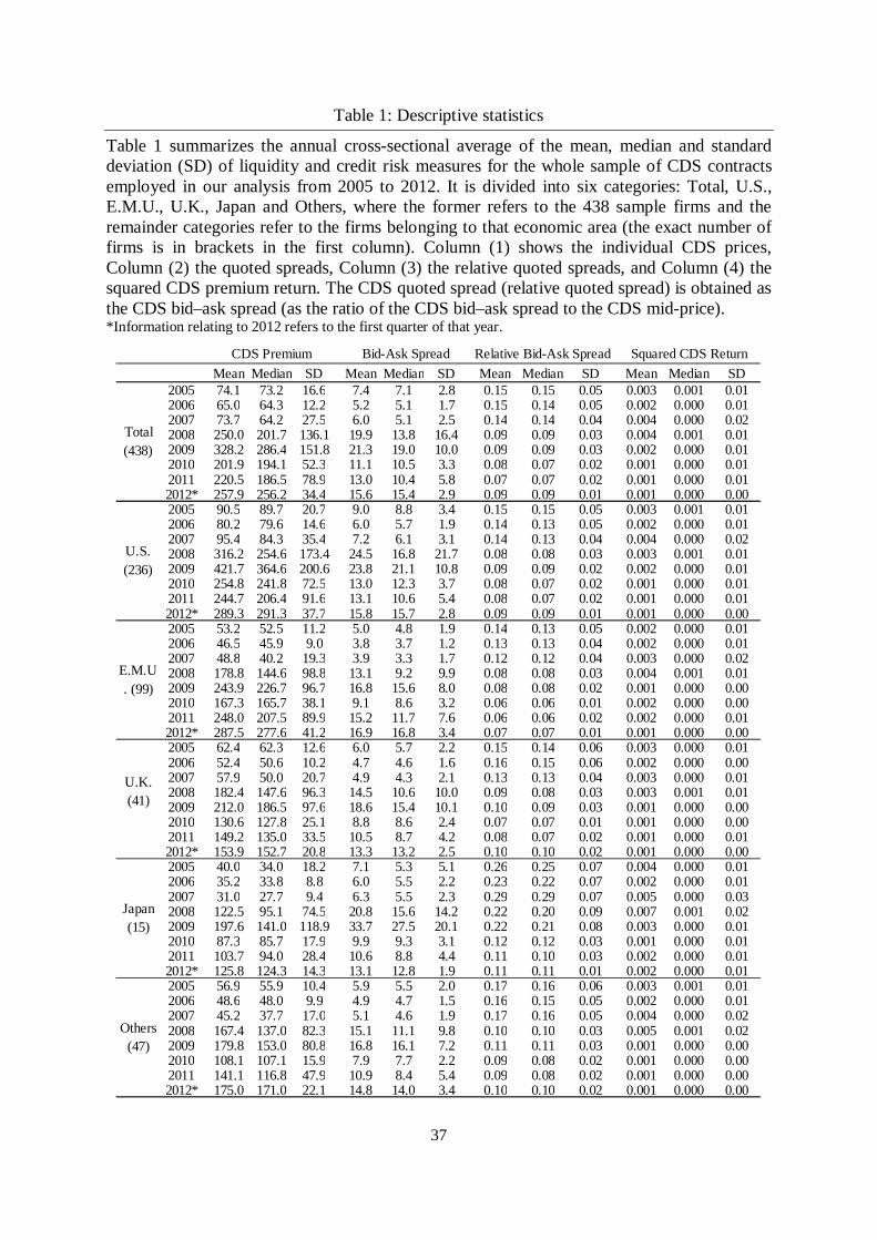
37

Table 1: Descriptive statistics

Table 1 summarizes the annual cross-sectional average of the mean, median and standard deviation (SD) of liquidity and credit risk measures for the whole sample of CDS contracts employed in our analysis from 2005 to 2012. It is divided into six categories: Total, U.S., E.M.U., U.K., Japan and Others, where the former refers to the 438 sample firms and the remainder categories refer to the firms belonging to that economic area (the exact number of firms is in brackets in the first column). Column (1) shows the individual CDS prices, Column (2) the quoted spreads, Column (3) the relative quoted spreads, and Column (4) the squared CDS premium return. The CDS quoted spread (relative quoted spread) is obtained as the CDS bid–ask spread (as the ratio of the CDS bid–ask spread to the CDS mid-price). *Information relating to 2012 refers to the first quarter of that year.

Mean Median SD Mean Median SD Mean Median SD Mean Median SD2005 74.1 73.2 16.6 7.4 7.1 2.8 0.15 0.15 0.05 0.003 0.001 0.012006 65.0 64.3 12.2 5.2 5.1 1.7 0.15 0.14 0.05 0.002 0.000 0.012007 73.7 64.2 27.5 6.0 5.1 2.5 0.14 0.14 0.04 0.004 0.000 0.022008 250.0 201.7 136.1 19.9 13.8 16.4 0.09 0.09 0.03 0.004 0.001 0.012009 328.2 286.4 151.8 21.3 19.0 10.0 0.09 0.09 0.03 0.002 0.000 0.012010 201.9 194.1 52.3 11.1 10.5 3.3 0.08 0.07 0.02 0.001 0.000 0.012011 220.5 186.5 78.9 13.0 10.4 5.8 0.07 0.07 0.02 0.001 0.000 0.012012* 257.9 256.2 34.4 15.6 15.4 2.9 0.09 0.09 0.01 0.001 0.000 0.002005 90.5 89.7 20.7 9.0 8.8 3.4 0.15 0.15 0.05 0.003 0.001 0.012006 80.2 79.6 14.6 6.0 5.7 1.9 0.14 0.13 0.05 0.002 0.000 0.012007 95.4 84.3 35.4 7.2 6.1 3.1 0.14 0.13 0.04 0.004 0.000 0.022008 316.2 254.6 173.4 24.5 16.8 21.7 0.08 0.08 0.03 0.003 0.001 0.012009 421.7 364.6 200.6 23.8 21.1 10.8 0.09 0.09 0.02 0.002 0.000 0.012010 254.8 241.8 72.5 13.0 12.3 3.7 0.08 0.07 0.02 0.001 0.000 0.012011 244.7 206.4 91.6 13.1 10.6 5.4 0.08 0.07 0.02 0.001 0.000 0.012012* 289.3 291.3 37.7 15.8 15.7 2.8 0.09 0.09 0.01 0.001 0.000 0.002005 53.2 52.5 11.2 5.0 4.8 1.9 0.14 0.13 0.05 0.002 0.000 0.012006 46.5 45.9 9.0 3.8 3.7 1.2 0.13 0.13 0.04 0.002 0.000 0.012007 48.8 40.2 19.3 3.9 3.3 1.7 0.12 0.12 0.04 0.003 0.000 0.022008 178.8 144.6 98.8 13.1 9.2 9.9 0.08 0.08 0.03 0.004 0.001 0.012009 243.9 226.7 96.7 16.8 15.6 8.0 0.08 0.08 0.02 0.001 0.000 0.002010 167.3 165.7 38.1 9.1 8.6 3.2 0.06 0.06 0.01 0.002 0.000 0.002011 248.0 207.5 89.9 15.2 11.7 7.6 0.06 0.06 0.02 0.002 0.000 0.012012* 287.5 277.6 41.2 16.9 16.8 3.4 0.07 0.07 0.01 0.001 0.000 0.002005 62.4 62.3 12.6 6.0 5.7 2.2 0.15 0.14 0.06 0.003 0.000 0.012006 52.4 50.6 10.2 4.7 4.6 1.6 0.16 0.15 0.06 0.002 0.000 0.002007 57.9 50.0 20.7 4.9 4.3 2.1 0.13 0.13 0.04 0.003 0.000 0.012008 182.4 147.6 96.3 14.5 10.6 10.0 0.09 0.08 0.03 0.003 0.001 0.012009 212.0 186.5 97.6 18.6 15.4 10.1 0.10 0.09 0.03 0.001 0.000 0.002010 130.6 127.8 25.1 8.8 8.6 2.4 0.07 0.07 0.01 0.001 0.000 0.002011 149.2 135.0 33.5 10.5 8.7 4.2 0.08 0.07 0.02 0.001 0.000 0.012012* 153.9 152.7 20.8 13.3 13.2 2.5 0.10 0.10 0.02 0.001 0.000 0.002005 40.0 34.0 18.2 7.1 5.3 5.1 0.26 0.25 0.07 0.004 0.000 0.012006 35.2 33.8 8.8 6.0 5.5 2.2 0.23 0.22 0.07 0.002 0.000 0.012007 31.0 27.7 9.4 6.3 5.5 2.3 0.29 0.29 0.07 0.005 0.000 0.032008 122.5 95.1 74.5 20.8 15.6 14.2 0.22 0.20 0.09 0.007 0.001 0.022009 197.6 141.0 118.9 33.7 27.5 20.1 0.22 0.21 0.08 0.003 0.000 0.012010 87.3 85.7 17.9 9.9 9.3 3.1 0.12 0.12 0.03 0.001 0.000 0.012011 103.7 94.0 28.4 10.6 8.8 4.4 0.11 0.10 0.03 0.002 0.000 0.012012* 125.8 124.3 14.3 13.1 12.8 1.9 0.11 0.11 0.01 0.002 0.000 0.012005 56.9 55.9 10.4 5.9 5.5 2.0 0.17 0.16 0.06 0.003 0.001 0.012006 48.6 48.0 9.9 4.9 4.7 1.5 0.16 0.15 0.05 0.002 0.000 0.012007 45.2 37.7 17.0 5.1 4.6 1.9 0.17 0.16 0.05 0.004 0.000 0.022008 167.4 137.0 82.3 15.1 11.1 9.8 0.10 0.10 0.03 0.005 0.001 0.022009 179.8 153.0 80.8 16.8 16.1 7.2 0.11 0.11 0.03 0.001 0.000 0.002010 108.1 107.1 15.9 7.9 7.7 2.2 0.09 0.08 0.02 0.001 0.000 0.002011 141.1 116.8 47.9 10.9 8.4 5.4 0.09 0.08 0.02 0.001 0.000 0.002012* 175.0 171.0 22.1 14.8 14.0 3.4 0.10 0.10 0.02 0.001 0.000 0.00

U.K. (41)

Japan (15)

Others (47)

CDS Premium Bid-Ask Spread Relative Bid-Ask Spread

Total (438)

U.S. (236)

E.M.U. (99)

Squared CDS Return

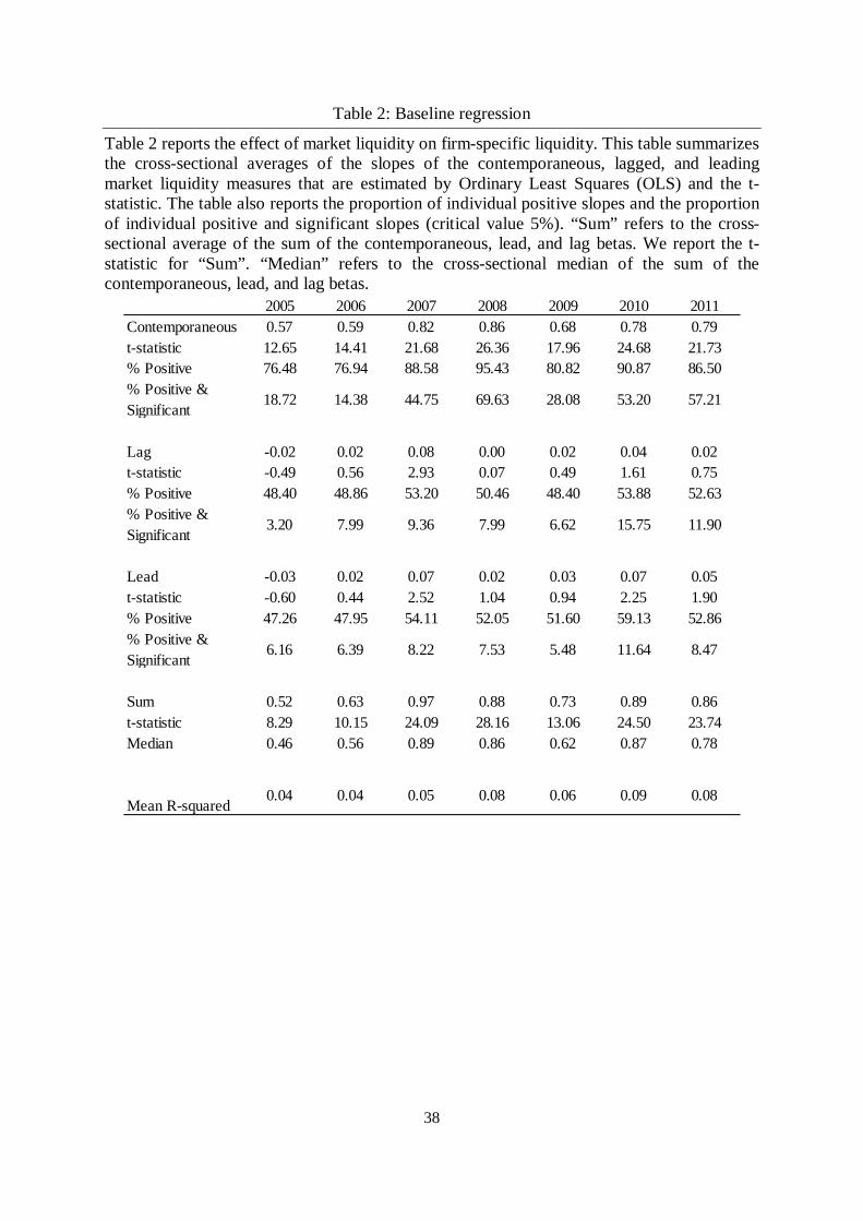
38

Table 2: Baseline regression

Table 2 reports the effect of market liquidity on firm-specific liquidity. This table summarizes the cross-sectional averages of the slopes of the contemporaneous, lagged, and leading market liquidity measures that are estimated by Ordinary Least Squares (OLS) and the t-statistic. The table also reports the proportion of individual positive slopes and the proportion of individual positive and significant slopes (critical value 5%). “Sum” refers to the cross-sectional average of the sum of the contemporaneous, lead, and lag betas. We report the t-statistic for “Sum”. “Median” refers to the cross-sectional median of the sum of the contemporaneous, lead, and lag betas.

2005 2006 2007 2008 2009 2010 2011Contemporaneous 0.57 0.59 0.82 0.86 0.68 0.78 0.79t-statistic 12.65 14.41 21.68 26.36 17.96 24.68 21.73% Positive 76.48 76.94 88.58 95.43 80.82 90.87 86.50% Positive & Significant

18.72 14.38 44.75 69.63 28.08 53.20 57.21

Lag -0.02 0.02 0.08 0.00 0.02 0.04 0.02t-statistic -0.49 0.56 2.93 0.07 0.49 1.61 0.75% Positive 48.40 48.86 53.20 50.46 48.40 53.88 52.63% Positive & Significant

3.20 7.99 9.36 7.99 6.62 15.75 11.90

Lead -0.03 0.02 0.07 0.02 0.03 0.07 0.05t-statistic -0.60 0.44 2.52 1.04 0.94 2.25 1.90% Positive 47.26 47.95 54.11 52.05 51.60 59.13 52.86% Positive & Significant

6.16 6.39 8.22 7.53 5.48 11.64 8.47

Sum 0.52 0.63 0.97 0.88 0.73 0.89 0.86t-statistic 8.29 10.15 24.09 28.16 13.06 24.50 23.74Median 0.46 0.56 0.89 0.86 0.62 0.87 0.78

Mean R-squared0.04 0.04 0.05 0.08 0.06 0.09 0.08

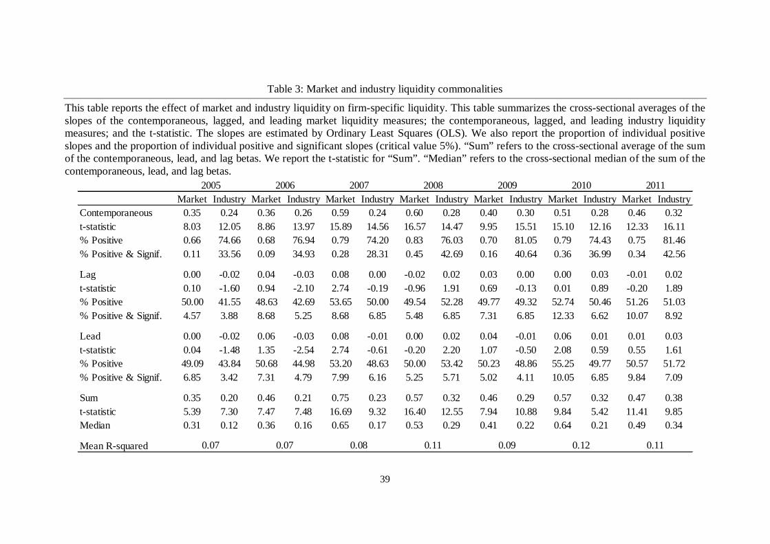
39

Table 3: Market and industry liquidity commonalities

This table reports the effect of market and industry liquidity on firm-specific liquidity. This table summarizes the cross-sectional averages of the slopes of the contemporaneous, lagged, and leading market liquidity measures; the contemporaneous, lagged, and leading industry liquidity measures; and the t-statistic. The slopes are estimated by Ordinary Least Squares (OLS). We also report the proportion of individual positive slopes and the proportion of individual positive and significant slopes (critical value 5%). “Sum” refers to the cross-sectional average of the sum of the contemporaneous, lead, and lag betas. We report the t-statistic for “Sum”. “Median” refers to the cross-sectional median of the sum of the contemporaneous, lead, and lag betas.

Market Industry Market Industry Market Industry Market Industry Market Industry Market Industry Market IndustryContemporaneous 0.35 0.24 0.36 0.26 0.59 0.24 0.60 0.28 0.40 0.30 0.51 0.28 0.46 0.32t-statistic 8.03 12.05 8.86 13.97 15.89 14.56 16.57 14.47 9.95 15.51 15.10 12.16 12.33 16.11% Positive 0.66 74.66 0.68 76.94 0.79 74.20 0.83 76.03 0.70 81.05 0.79 74.43 0.75 81.46% Positive & Signif. 0.11 33.56 0.09 34.93 0.28 28.31 0.45 42.69 0.16 40.64 0.36 36.99 0.34 42.56

Lag 0.00 -0.02 0.04 -0.03 0.08 0.00 -0.02 0.02 0.03 0.00 0.00 0.03 -0.01 0.02t-statistic 0.10 -1.60 0.94 -2.10 2.74 -0.19 -0.96 1.91 0.69 -0.13 0.01 0.89 -0.20 1.89% Positive 50.00 41.55 48.63 42.69 53.65 50.00 49.54 52.28 49.77 49.32 52.74 50.46 51.26 51.03% Positive & Signif. 4.57 3.88 8.68 5.25 8.68 6.85 5.48 6.85 7.31 6.85 12.33 6.62 10.07 8.92

Lead 0.00 -0.02 0.06 -0.03 0.08 -0.01 0.00 0.02 0.04 -0.01 0.06 0.01 0.01 0.03t-statistic 0.04 -1.48 1.35 -2.54 2.74 -0.61 -0.20 2.20 1.07 -0.50 2.08 0.59 0.55 1.61% Positive 49.09 43.84 50.68 44.98 53.20 48.63 50.00 53.42 50.23 48.86 55.25 49.77 50.57 51.72% Positive & Signif. 6.85 3.42 7.31 4.79 7.99 6.16 5.25 5.71 5.02 4.11 10.05 6.85 9.84 7.09

Sum 0.35 0.20 0.46 0.21 0.75 0.23 0.57 0.32 0.46 0.29 0.57 0.32 0.47 0.38t-statistic 5.39 7.30 7.47 7.48 16.69 9.32 16.40 12.55 7.94 10.88 9.84 5.42 11.41 9.85Median 0.31 0.12 0.36 0.16 0.65 0.17 0.53 0.29 0.41 0.22 0.64 0.21 0.49 0.34

Mean R-squared

2011

0.07 0.07 0.08 0.11 0.09 0.12 0.11

2005 2006 2007 2008 2009 2010

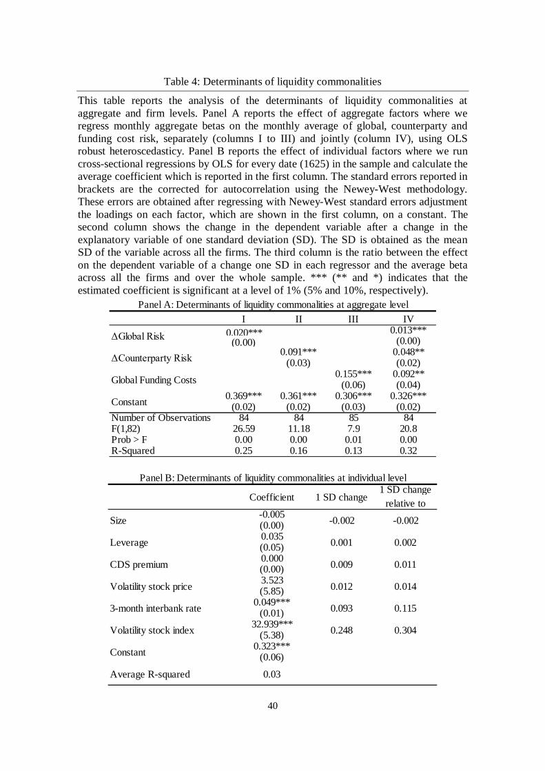
40

Table 4: Determinants of liquidity commonalities

This table reports the analysis of the determinants of liquidity commonalities at aggregate and firm levels. Panel A reports the effect of aggregate factors where we regress monthly aggregate betas on the monthly average of global, counterparty and funding cost risk, separately (columns I to III) and jointly (column IV), using OLS robust heteroscedasticy. Panel B reports the effect of individual factors where we run cross-sectional regressions by OLS for every date (1625) in the sample and calculate the average coefficient which is reported in the first column. The standard errors reported in brackets are the corrected for autocorrelation using the Newey-West methodology. These errors are obtained after regressing with Newey-West standard errors adjustment the loadings on each factor, which are shown in the first column, on a constant. The second column shows the change in the dependent variable after a change in the explanatory variable of one standard deviation (SD). The SD is obtained as the mean SD of the variable across all the firms. The third column is the ratio between the effect on the dependent variable of a change one SD in each regressor and the average beta across all the firms and over the whole sample. *** (** and *) indicates that the estimated coefficient is significant at a level of 1% (5% and 10%, respectively).

I II III IV 0.020*** 0.013***

(0.00) (0.00)0.091*** 0.048**

(0.03) (0.02)0.155*** 0.092**

(0.06) (0.04)0.369*** 0.361*** 0.306*** 0.326***

(0.02) (0.02) (0.03) (0.02)Number of Observations 84 84 85 84F(1,82) 26.59 11.18 7.9 20.8Prob > F 0.00 0.00 0.01 0.00R-Squared 0.25 0.16 0.13 0.32

ΔGlobal Risk

ΔCounterparty Risk

Global Funding Costs

Constant

Panel A: Determinants of liquidity commonalities at aggregate level

-0.005(0.00)0.035(0.05)0.000(0.00)3.523(5.85)

0.049***(0.01)

32.939***(5.38)

0.323***(0.06)Constant

Panel B: Determinants of liquidity commonalities at individual level

0.012 0.014

0.093 0.115

1 SD change relative to

Average R-squared

-0.002 -0.002

0.001 0.002

0.009 0.011

Size

Leverage

CDS premium

Volatility stock price

0.03

0.248 0.304

3-month interbank rate

Volatility stock index

Coefficient 1 SD change

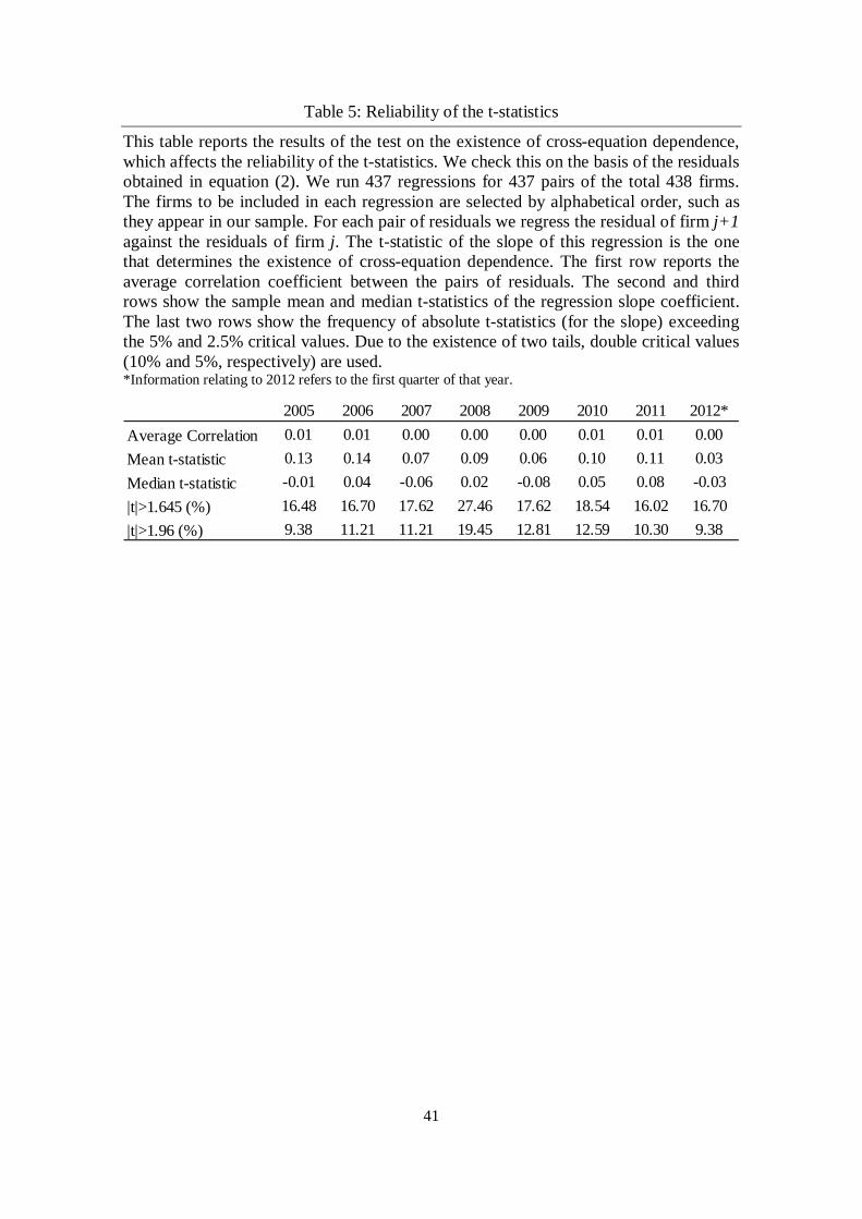
41

Table 5: Reliability of the t-statistics

This table reports the results of the test on the existence of cross-equation dependence, which affects the reliability of the t-statistics. We check this on the basis of the residuals obtained in equation (2). We run 437 regressions for 437 pairs of the total 438 firms. The firms to be included in each regression are selected by alphabetical order, such as they appear in our sample. For each pair of residuals we regress the residual of firm j+1 against the residuals of firm j. The t-statistic of the slope of this regression is the one that determines the existence of cross-equation dependence. The first row reports the average correlation coefficient between the pairs of residuals. The second and third rows show the sample mean and median t-statistics of the regression slope coefficient. The last two rows show the frequency of absolute t-statistics (for the slope) exceeding the 5% and 2.5% critical values. Due to the existence of two tails, double critical values (10% and 5%, respectively) are used. *Information relating to 2012 refers to the first quarter of that year.

2005 2006 2007 2008 2009 2010 2011 2012*Average Correlation 0.01 0.01 0.00 0.00 0.00 0.01 0.01 0.00Mean t-statistic 0.13 0.14 0.07 0.09 0.06 0.10 0.11 0.03Median t-statistic -0.01 0.04 -0.06 0.02 -0.08 0.05 0.08 -0.03|t|>1.645 (%) 16.48 16.70 17.62 27.46 17.62 18.54 16.02 16.70|t|>1.96 (%) 9.38 11.21 11.21 19.45 12.81 12.59 10.30 9.38

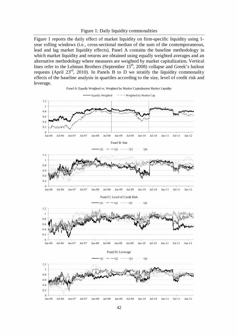
42

Figure 1: Daily liquidity commonalities

Figure 1 reports the daily effect of market liquidity on firm-specific liquidity using 1-year rolling windows (i.e., cross-sectional median of the sum of the contemporaneous, lead and lag market liquidity effects). Panel A contains the baseline methodology in which market liquidity and returns are obtained using equally weighted averages and an alternative methodology where measures are weighted by market capitalization. Vertical lines refer to the Lehman Brothers (September 15th, 2008) collapse and Greek’s bailout requests (April 23rd, 2010). In Panels B to D we stratify the liquidity commonality effects of the baseline analysis in quartiles according to the size, level of credit risk and leverage.

Panel A: Equally Weighted vs. Weighted by Market Capitalization Market Liquidity

Panel B: Size

Panel C: Level of Credit Risk

Panel D: Leverage

0

0.2

0.4

0.6

0.8

1

1.2

Jan-06 Jul-06 Jan-07 Jul-07 Jan-08 Jul-08 Jan-09 Jul-09 Jan-10 Jul-10 Jan-11 Jul-11 Jan-12

Equally Weighted Weighted by Market Cap.

0

0.2

0.4

0.6

0.8

1

1.2

Jan-06 Jul-06 Jan-07 Jul-07 Jan-08 Jul-08 Jan-09 Jul-09 Jan-10 Jul-10 Jan-11 Jul-11 Jan-12

Q1 Q2 Q3 Q4

0

0.2

0.4

0.6

0.8

1

1.2

Jan-06 Jul-06 Jan-07 Jul-07 Jan-08 Jul-08 Jan-09 Jul-09 Jan-10 Jul-10 Jan-11 Jul-11 Jan-12

Q1 Q2 Q3 Q4

0

0.2

0.4

0.6

0.8

1

1.2

Jan-06 Jul-06 Jan-07 Jul-07 Jan-08 Jul-08 Jan-09 Jul-09 Jan-10 Jul-10 Jan-11 Jul-11 Jan-12

Q1 Q2 Q3 Q4

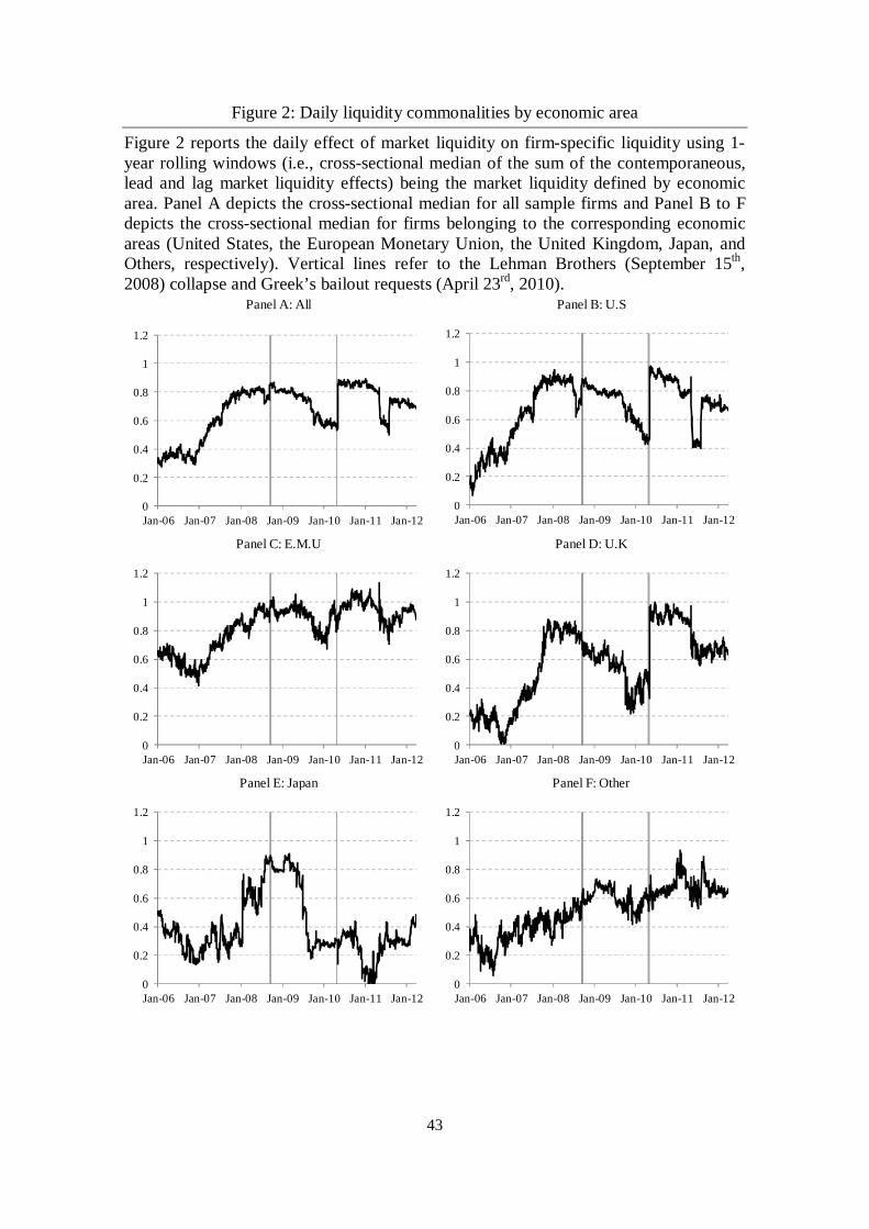
43

Figure 2: Daily liquidity commonalities by economic area

Figure 2 reports the daily effect of market liquidity on firm-specific liquidity using 1-year rolling windows (i.e., cross-sectional median of the sum of the contemporaneous, lead and lag market liquidity effects) being the market liquidity defined by economic area. Panel A depicts the cross-sectional median for all sample firms and Panel B to F depicts the cross-sectional median for firms belonging to the corresponding economic areas (United States, the European Monetary Union, the United Kingdom, Japan, and Others, respectively). Vertical lines refer to the Lehman Brothers (September 15th, 2008) collapse and Greek’s bailout requests (April 23rd, 2010).

Panel A: All Panel B: U.S

Panel C: E.M.U Panel D: U.K

Panel E: Japan Panel F: Other

0

0.2

0.4

0.6

0.8

1

1.2

Jan-06 Jan-07 Jan-08 Jan-09 Jan-10 Jan-11 Jan-120

0.2

0.4

0.6

0.8

1

1.2

Jan-06 Jan-07 Jan-08 Jan-09 Jan-10 Jan-11 Jan-12

0

0.2

0.4

0.6

0.8

1

1.2

Jan-06 Jan-07 Jan-08 Jan-09 Jan-10 Jan-11 Jan-120

0.2

0.4

0.6

0.8

1

1.2

Jan-06 Jan-07 Jan-08 Jan-09 Jan-10 Jan-11 Jan-12

0

0.2

0.4

0.6

0.8

1

1.2

Jan-06 Jan-07 Jan-08 Jan-09 Jan-10 Jan-11 Jan-120

0.2

0.4

0.6

0.8

1

1.2

Jan-06 Jan-07 Jan-08 Jan-09 Jan-10 Jan-11 Jan-12

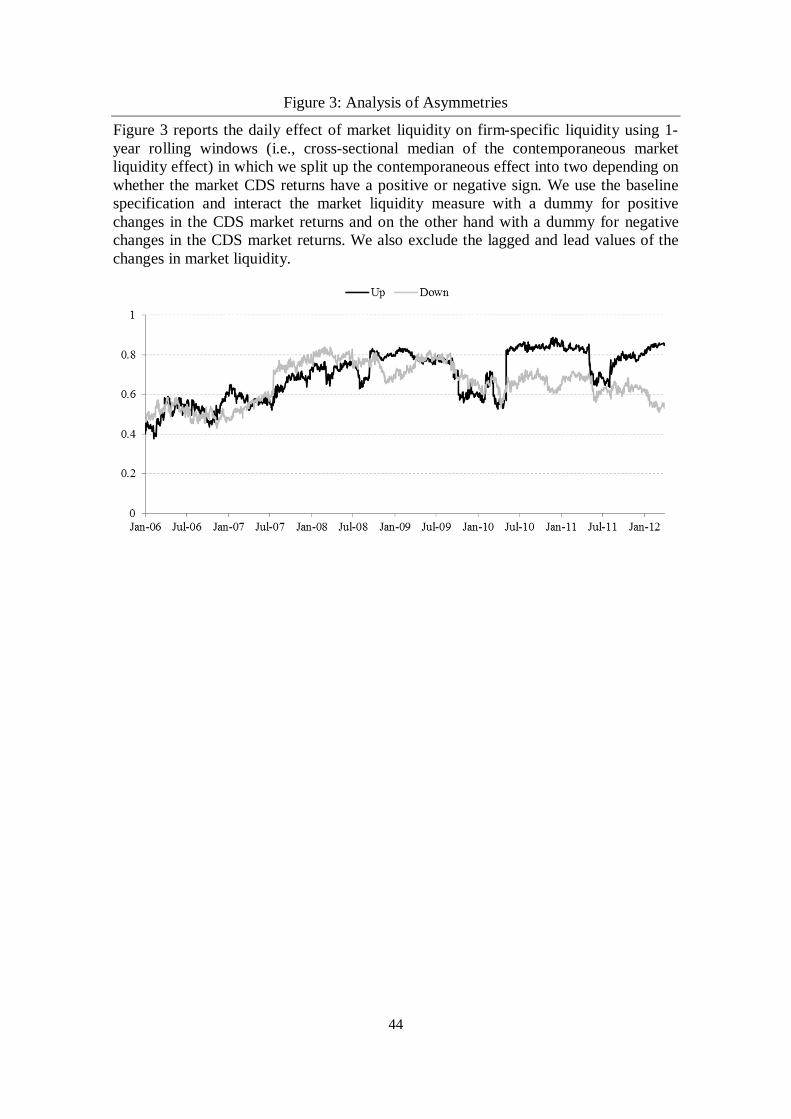
44

Figure 3: Analysis of Asymmetries

Figure 3 reports the daily effect of market liquidity on firm-specific liquidity using 1-year rolling windows (i.e., cross-sectional median of the contemporaneous market liquidity effect) in which we split up the contemporaneous effect into two depending on whether the market CDS returns have a positive or negative sign. We use the baseline specification and interact the market liquidity measure with a dummy for positive changes in the CDS market returns and on the other hand with a dummy for negative changes in the CDS market returns. We also exclude the lagged and lead values of the changes in market liquidity.

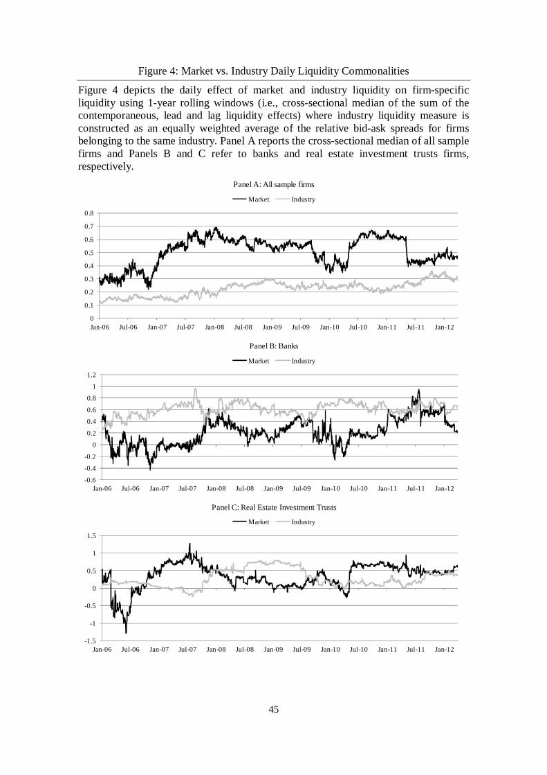
45

Figure 4: Market vs. Industry Daily Liquidity Commonalities

Figure 4 depicts the daily effect of market and industry liquidity on firm-specific liquidity using 1-year rolling windows (i.e., cross-sectional median of the sum of the contemporaneous, lead and lag liquidity effects) where industry liquidity measure is constructed as an equally weighted average of the relative bid-ask spreads for firms belonging to the same industry. Panel A reports the cross-sectional median of all sample firms and Panels B and C refer to banks and real estate investment trusts firms, respectively.

Panel B: Banks

Panel A: All sample firms

Panel C: Real Estate Investment Trusts

-1.5

-1

-0.5

0

0.5

1

1.5

Jan-06 Jul-06 Jan-07 Jul-07 Jan-08 Jul-08 Jan-09 Jul-09 Jan-10 Jul-10 Jan-11 Jul-11 Jan-12

Market Industry

-0.6

-0.4

-0.2

0

0.2

0.4

0.6

0.8

1

1.2

Jan-06 Jul-06 Jan-07 Jul-07 Jan-08 Jul-08 Jan-09 Jul-09 Jan-10 Jul-10 Jan-11 Jul-11 Jan-12

Market Industry

0

0.1

0.2

0.3

0.4

0.5

0.6

0.7

0.8

Jan-06 Jul-06 Jan-07 Jul-07 Jan-08 Jul-08 Jan-09 Jul-09 Jan-10 Jul-10 Jan-11 Jul-11 Jan-12

Market Industry

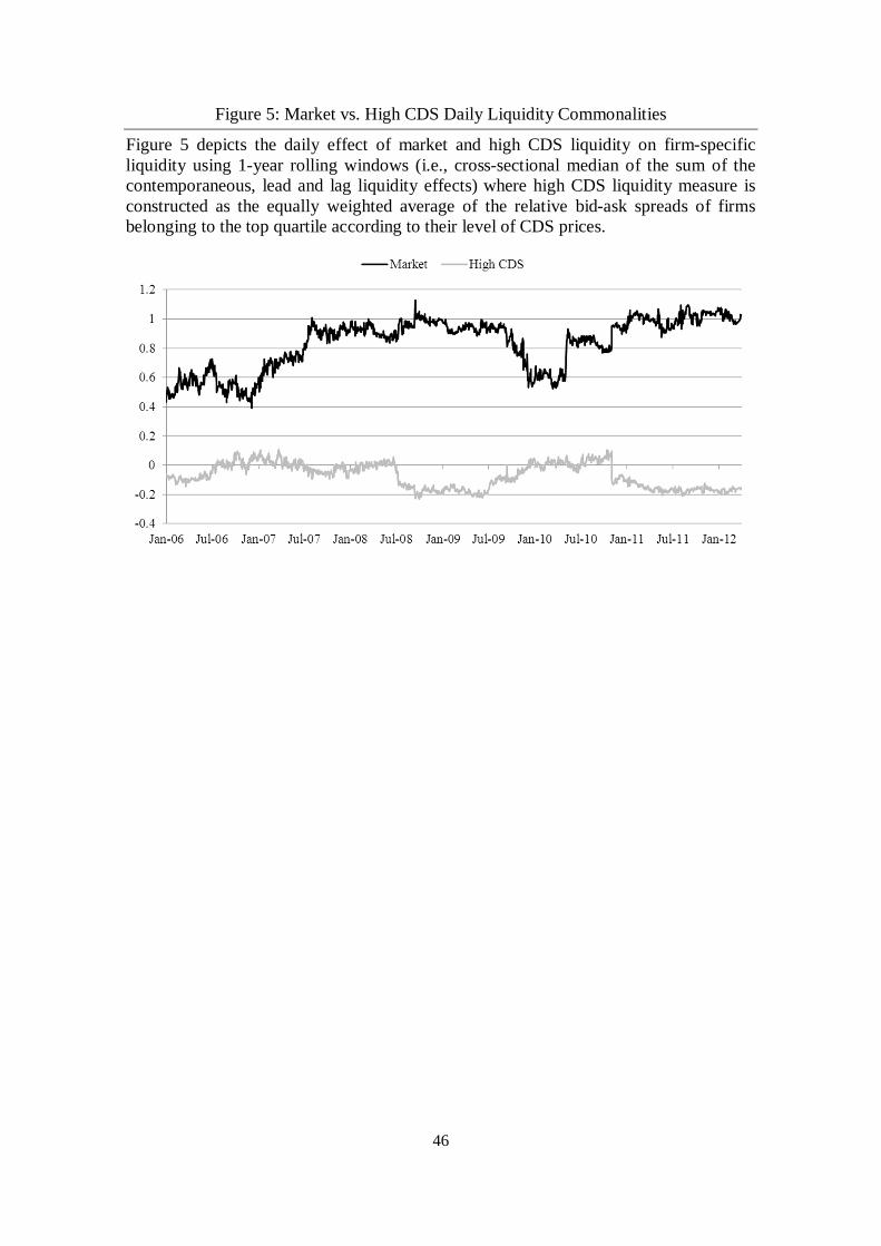
46

Figure 5: Market vs. High CDS Daily Liquidity Commonalities

Figure 5 depicts the daily effect of market and high CDS liquidity on firm-specific liquidity using 1-year rolling windows (i.e., cross-sectional median of the sum of the contemporaneous, lead and lag liquidity effects) where high CDS liquidity measure is constructed as the equally weighted average of the relative bid-ask spreads of firms belonging to the top quartile according to their level of CDS prices.

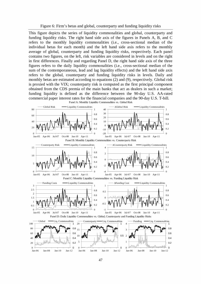
47

Figure 6: Firm’s betas and global, counterparty and funding liquidity risks

This figure depicts the series of liquidity commonalities and global, counterparty and funding liquidity risks. The right hand side axis of the figures in Panels A, B, and C refers to the monthly liquidity commonalities (i.e., cross-sectional median of the individual betas for each month) and the left hand side axis refers to the monthly average of global, counterparty and funding liquidity risks, respectively. Each panel contains two figures, on the left, risk variables are considered in levels and on the right in first differences. Finally and regarding Panel D, the right hand side axis of the three figures refers to the daily liquidity commonalities (i.e., cross-sectional median of the sum of the contemporaneous, lead and lag liquidity effects) and the left hand side axis refers to the global, counterparty and funding liquidity risks in levels. Daily and monthly betas are estimated according to equations (2) and (9), respectively. Global risk is proxied with the VIX; counterparty risk is computed as the first principal component obtained from the CDS premia of the main banks that act as dealers in such a market; funding liquidity is defined as the difference between the 90-day U.S. AA-rated commercial paper interest rates for the financial companies and the 90-day U.S. T-bill.

Panel A: Monthly Liquidity Commonalities vs. Global Risk

Panel B: Monthly Liquidity Commonalities vs. Counterparty Risk

Panel C: Monthly Liquidity Commonalities vs. Funding Liquidity Risk

Panel D: Daily Liquidity Commonalities vs. Global, Counterparty and Funding Liquidity Risks

0

0.2

0.4

0.6

0.8

1

0

0.51

1.5

22.5

3

Jan-05 Apr-06 Jul-07 Oct-08 Jan-10 Apr-11

Funding Costs Liquidity Commonalities

0

0.2

0.4

0.6

0.8

1

-1

-0.5

0

0.5

1

Jan-05 Apr-06 Jul-07 Oct-08 Jan-10 Apr-11

ΔFunding Cost Liquidity Commonalities

0

0.2

0.4

0.6

0.8

1

0

20

40

60

80

100

Jan-06 Jan-08 Jan-10 Jan-12

Global Liq. Commonalities

0

0.5

1

0

5

10

15

20

Jan-06 Jan-08 Jan-10 Jan-12

Counterparty Liq. Commonalities

0

0.2

0.4

0.6

0.8

1

0

1

2

3

4

Jan-06 Jan-08 Jan-10 Jan-12

Funding Liq. Commonalities

0

0.2

0.4

0.6

0.8

1

0

20

40

60

80

Jan-05 Apr-06 Jul-07 Oct-08 Jan-10 Apr-11

Global Risk Liquidity Commonalities

0

0.2

0.4

0.6

0.8

1

-20-10

010

2030

40

Jan-05 Apr-06 Jul-07 Oct-08 Jan-10 Apr-11

ΔGlobal Risk Liquidity Commonalities

0

0.2

0.4

0.6

0.8

1

0

5

10

15

Jan-05 Apr-06 Jul-07 Oct-08 Jan-10 Apr-11

Counterparty Risk Liquidity Commonalities

0

0.2

0.4

0.6

0.8

1

-4

-2

0

2

4

Jan-05 Apr-06 Jul-07 Oct-08 Jan-10 Apr-11

ΔCounterparty Risk Liquidity Commonalities

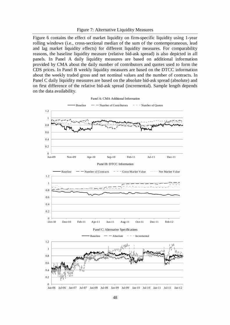
48

Figure 7: Alternative Liquidity Measures

Figure 6 contains the effect of market liquidity on firm-specific liquidity using 1-year rolling windows (i.e., cross-sectional median of the sum of the contemporaneous, lead and lag market liquidity effects) for different liquidity measures. For comparability reasons, the baseline liquidity measure (relative bid-ask spread) is also depicted in all panels. In Panel A daily liquidity measures are based on additional information provided by CMA about the daily number of contributors and quotes used to form the CDS prices. In Panel B weekly liquidity measures are based on the DTCC information about the weekly traded gross and net nominal values and the number of contracts. In Panel C daily liquidity measures are based on the absolute bid-ask spread (absolute) and on first difference of the relative bid-ask spread (incremental). Sample length depends on the data availability.

Panel A: CMA Additional Information

Panel B: DTCC Information

Panel C: Alternative Specifications

0

0.2

0.4

0.6

0.8

1

1.2

Jun-09 Nov-09 Apr-10 Sep-10 Feb-11 Jul-11 Dec-11

Baseline Number of Contributors Number of Quotes

0

0.2

0.4

0.6

0.8

1

1.2

Oct-10 Dec-10 Feb-11 Apr-11 Jun-11 Aug-11 Oct-11 Dec-11 Feb-12

Baseline Number of Contracts Gross Market Value Net Market Value

0

0.2

0.4

0.6

0.8

1

1.2

Jan-06 Jul-06 Jan-07 Jul-07 Jan-08 Jul-08 Jan-09 Jul-09 Jan-10 Jul-10 Jan-11 Jul-11 Jan-12

Baseline Absolute Incremental

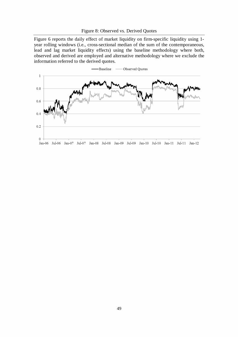
49

Figure 8: Observed vs. Derived Quotes

Figure 6 reports the daily effect of market liquidity on firm-specific liquidity using 1-year rolling windows (i.e., cross-sectional median of the sum of the contemporaneous, lead and lag market liquidity effects) using the baseline methodology where both, observed and derived are employed and alternative methodology where we exclude the information referred to the derived quotes.