1

Working with Project Files in ArcGIS and HEC-RAS

Prepared by Cassandra Fagan and David Maidment

CE 365K Hydraulic Engineering Design

Spring 2016

Contents (1) View the spatial files in ArcGIS ........................................................................................... 1

(2) Delineate the Drainage Area of your Project Site ................................................................. 8

(3) Open the hydraulic model in HEC-RAS ............................................................................. 14

(1) View the spatial files in ArcGIS

The models and spatial files may be found in the following folder. If you are accessing this from

a remote computer, you’ll have to use VPN to connect to UT first.

\\austin.utexas.edu\disk\engrstu\class\caee\ce365k\CE365K2016

Navigate to this folder and download the model and spatial files corresponding to your site.

The Boggy Creek folder contains the City of Austin’s official HEC-RAS model for Boggy Creek.

The Boggy Creek Spatial folder contains spatial data for Boggy Creek that may be viewed using

ArcGIS.

To explore additional data available from the City of Austin visit: www.austintexas.gov/floodpro/

Open ArcMap , , and select “cancel” when the “ ArcMap – Getting Started” prompt

appears, seen below.

2

Navigate to File Map Document Properties, and check the box next to “Store relative

pathnames to data sources”.

Then if you keep the map document and its data in the same folder and move the entire folder

between computers the references to the data in the map persist.

Next, let’s save our map document. Navigate to File, and select save as Boggy.mxd.

3

Next, add the Spatial files to the ArcMap Display. Select the Add Data icon, seen below.

In the Add Data pop-up window select “connect to folder”.

Navigate to the folder where your spatial files are stored and select add.

Select the spatial files you wish to add to the ArcMap display.

4

.

Now you can view the modeled reach, its cross-sections, and various floodplains.

You can turn layers on, and off by clicking on the check mark next to the layer’s name.

5

If you want to make the display more interesting, select Add Data, and choose Add

Basemap. The Streets and Topographic maps are helpful for understanding the location of your

site on the modeled river.

Go to the project data folder and get the folder Project Sites

6

Use Add Data to add the ProjectSites shape file to your ArcMap display

And you’ll see a ProjectSites feature class displayed

Which has a small dot to show your site. Click on this dot to open the Symbol Selector, and

make your dot larger so that you can see it more clearly on the map.

7

The pan, zoom in, and zoom out tools, , are helpful to navigate to the site location.

Once you have located your site use the identify tool, , to identify which cross-sections in

the model correspond to the inlet and outlet on your site. Right-click on the cross-sections

using the identify tool. This tells us that the inlet to the structure located at the intersection of

Boggy Creek, and Delwau Lane bounded by cross-sections 3208 and 3118.

8

(2) Delineate the Drainage Area of your Project Site

In ArcMap, sign in to your UT Austin Organizational Account

In ArcCatalog (tab on right hand side of ArcMap document), expand the “Ready to Use

Services” to find the Watershed function

9

Click on this Watershed function, and in the open window, select a Snap Distance of 100 meters,

the FINEST source resolution data then move the cursor to the Project Sites point and click on it,

then say OK in the Watershed window. It takes a little bit for this function to run (you are

10

accessing digital terrain data in the cloud to facilitate this).

You’ll see two new feature classes added to your project legend, Output Snapped Points and

Output Watershed. If you right click on Output Watershed and select Zoom to Layer, you’ll see

the drainage area of your project site. Pretty cool!!

Let’s create a storage location for your project watershed.

Right click on the folder where you project files are stored in Arc Catalog, and select New File

Geodatabase

11

And name it Project.gdb. Then right click on the resulting Project Geodatabase and establish a

new Feature Dataset

Name the resulting Feature Dataset BoggyCk or whatever you want, and in the next screen,

navigate to the bottom of the display and in the folder called “Layers” select the Central Texas

State Plane Coordinate System (the legal standard for work in this area).

12

Keep clicking until you hit Finish.

Now, lets put our Watershed into this Geodatabase. Right click on Output Watershed and

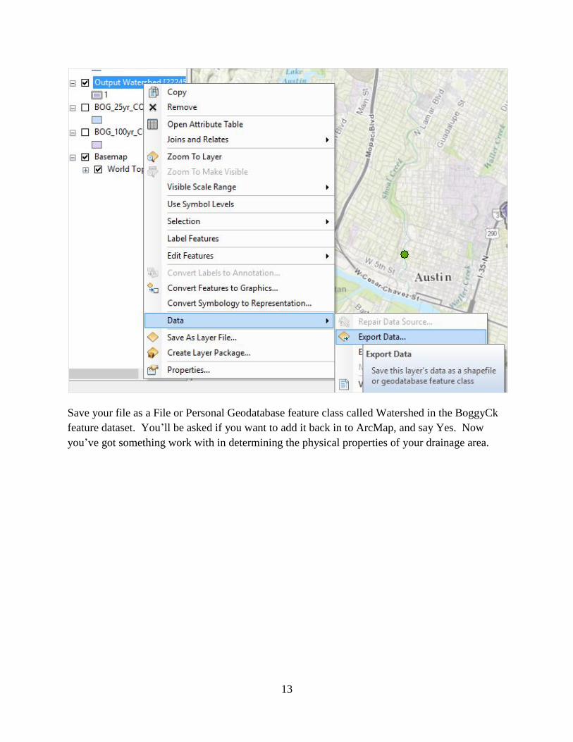
13

Save your file as a File or Personal Geodatabase feature class called Watershed in the BoggyCk

feature dataset. You’ll be asked if you want to add it back in to ArcMap, and say Yes. Now

you’ve got something work with in determining the physical properties of your drainage area.

14

If you right click on the Watershed feature class and open its Attribute table, you can find the

drainage area of your watershed:

Save your BoggyCk.mxd file using File/Save As in ArcMap to preserve your current project

outputs.

(3) Open the hydraulic model in HEC-RAS

Next we will open the creek model in HEC-RAS. This program is operational at the Learning

Resource Center. It can also be obtained directly from the Hydrologic Engineering Center at:

http://www.hec.usace.army.mil/software/hec-ras/ The latest version is HEC-RAS 5.0 which has

just come out. We’ll use HEC-RAS 4.1 because that is what is loaded at the LRC. Navigate to

the folder containing the HEC-RAS model and if necessary, unzip it.

15

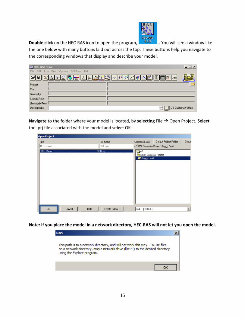
Double click on the HEC-RAS icon to open the program, . You will see a window like

the one below with many buttons laid out across the top. These buttons help you navigate to

the corresponding windows that display and describe your model.

Navigate to the folder where your model is located, by selecting File Open Project. Select

the .prj file associated with the model and select OK.

Note: If you place the model in a network directory, HEC-RAS will not let you open the model.

16

Once you have loaded the project you will see the Project name, file path, plan, and steady flow

files.

To view the profile of the reach:

(1) Click on the View profiles button, .

(2) Study the Profile Plot. What do you notice? The x-axis shows the distance upstream

from the most downstream cross section while the y-axis shows the elevation. The

legend shows the Energy Grade line, EG, the Water Surface line, WS, and Critical Depth

line, Crit.

(3) Close the Profile Plot window.

17

To view the cross sections along the reach:

(1) Click on the View cross sections button, .

(2) In the Cross Section window you can cycle through all the cross sections in the model by

clicking on the arrows next to River Sta. at the top of the window. Scan through the

Cross Sections until you find your site. Remember which river station is for later

reference.

(3) If you start at station 0 and move upstream, do you notice the water surface changing?

Like the Profile Plot, you will see the EG, WS and Crit lines plotted.

(4) Close the Cross Section window.

Finally, we can look at some rating curves created by HEC-RAS to gain a further understanding

of the analysis.

18

To view rating curves:

(1) In the main HEC-RAS window, click on the View General Rating Curve button, .

(2) The Rating Curve window will open and you will see a graph of the channel velocity as a

function of upstream distance. Navigate to your site’s rating curve. This will help you

understand the relationship between stage and discharge at your site.

19

Open the Bridge Output table:

(1) In the main HEC-RAS window, click on the Bridge Output button, .

(2) Navigate to your site’s Reach Section (RS).

(3) Change the profile to the storm you are designing for.

This table has information about the velocity, flow, and channel depth at your cross-section.

Save your HEC-RAS file before closing the program.