Embed Size (px)
Citation preview
WORLD HEALTH ORGANIZATION VACCINATION COVERAGE CLUSTER
SURVEYS: REFERENCE MANUAL

WORLD HEALTH ORGANIZATION VACCINATION COVERAGE CLUSTER
SURVEYS: REFERENCE MANUAL

Vaccination Coverage Cluster Surveys: Reference Manual.
Ordering code: WHO/IVB/18.09
Published: June 2018
© World Health Organization 2018
Some rights reserved. This work is available under the Creative Commons Attribution-NonCommercial-ShareAlike 3.0 IGO licence (CC BY-NC-SA 3.0 IGO; https://creativecommons.org/licenses/by-nc-sa/3.0/igo).
Under the terms of this licence, you may copy, redistribute and adapt the work for non-commercial purposes, provided the work is appropriately cited, as indicated below. In any use of this work, there should be no suggestion that WHO endorses any specific organization, products or services. The use of the WHO logo is not permitted. If you adapt the work, then you must license your work under the same or equivalent Creative Commons licence. If you create a translation of this work, you should add the following disclaimer along with the suggested citation: “This translation was not created by the World Health Organization (WHO). WHO is not responsible for the content or accuracy of this translation. The original English edition shall be the binding and authentic edition”.
Any mediation relating to disputes arising under the licence shall be conducted in accordance with the mediation rules of the World Intellectual Property Organization
Suggested citation. Vaccination Coverage Cluster Surveys: Reference Manual. Geneva: World Health Organization; 2018 (WHO/IVB/18.09). Licence: CC BY-NC-SA 3.0 IGO.
Cataloguing-in-Publication (CIP) data. CIP data are available at http://apps.who.int/iris.
Sales, rights and licensing. To purchase WHO publications, see http://apps.who.int/bookorders. To submit requests for commercial use and queries on rights and licensing, see http://www.who.int/about/licensing.
Third-party materials. If you wish to reuse material from this work that is attributed to a third party, such as tables, figures or images, it is your responsibility to determine whether permission is needed for that reuse and to obtain permission from the copyright holder. The risk of claims resulting from infringement of any third-party-owned component in the work rests solely with the user.
General disclaimers. The designations employed and the presentation of the material in this publication do not imply the expression of any opinion whatsoever on the part of WHO concerning the legal status of any country, territory, city or area or of its authorities, or concerning the delimitation of its frontiers or boundaries. Dotted and dashed lines on maps represent approximate border lines for which there may not yet be full agreement.
The mention of specific companies or of certain manufacturers’ products does not imply that they are endorsed or recommended by WHO in preference to others of a similar nature that are not mentioned. Errors and omissions excepted, the names of proprietary products are distinguished by initial capital letters.
All reasonable precautions have been taken by WHO to verify the information contained in this publication. However, the published material is being distributed without warranty of any kind, either expressed or implied. The responsibility for the interpretation and use of the material lies with the reader. In no event shall WHO be liable for damages arising from its use.
Design & layout: L’IV Com Sàrl, Villars-sous-Yens, Switzerland.
Printed in Switzerland.
iii
Contents
List of annexes iv Manual resources for each step of the survey process viList of boxes, figures and tables vii Abbreviations viii Acknowledgements ixPreface x1. Introduction 1
1.1. Why vaccination coverage is assessed 21.2. Methods for measuring vaccination coverage 21.3. Population-based surveys: cluster sampling 31.4. Changes to previous methods and materials 5
2. Design the sample structure of the survey 92.1. Convene a survey steering group 102.2. Discuss the purpose of the survey 112.3. Identify primary questions that affect survey design and sample size 112.4. Define the target population 122.5. Set inferential goals 122.6. Select a survey design 132.7. Calculate the required sample size 152.8. Draft an analysis plan, table shells and report figures 222.9. Budget for the survey and estimate the timeline 222.10. Evaluate affordability and timeliness 242.11. Implications of adding routine immunization questions to a post-SIA survey 252.12. Designing for multiple outcomes 262.13. Designing for multiple geographic areas 262.14. Designing for multiple levels of administrative or geographic hierarchy 262.15. Reporting results by subgroups 28
3. Make concrete plans 293.1. Set survey schedule 303.2. Decide who will conduct the survey and create a project plan 303.3. Obtain ethical clearance 313.4. Design data collection tools and methods 31

World Health Organization vaccination coverage cluster surveys: reference manual
iv
3.5. Choose data analysis tools 353.6. Select a sample 353.7. Obtain access to health registers for vaccination records 413.8. Select and hire staff 423.9. Train staff 46
4. Conduct field work 494.1. Collect data from households 504.2. Check health registers from the health centre 514.3. Monitor the quality of field data collection 524.4. Check questionnaire forms and transmit 534.5. Clusters that become suddenly inaccessible 54
5. Data entry, cleaning and management 555.1. Database design 565.2. Data entry 565.3. Clean the dataset 575.4. Merge datasets and construct derived variables 585.5. Generate a codebook 60
6. Tabulation and analysis 616.1. Conduct descriptive analyses to characterise the sample and assess its quality 626.2. Calculate weights for analysis 676.3. Conduct standard analyses 696.4. Conduct additional analyses 776.5. Classifying coverage 84
7. Interpret, format, and share results 897.1. Draft the background section 907.2. Draft the survey methods and limitations 917.3. Draft the results section 917.4. Draft the discussion section 937.5. Develop implications and recommendations 937.6. Revise the report and obtain clearance on final draft 967.7. Share the results 96
References 98
v
List of Annexes 100Annex A: Glossary of terms 100Annex B1: Steps to calculate a cluster survey sample size for estimation or classification 105Annex B2: Sample size equations for estimation or classification 129Annex B3: Sample size equations for comparisons between places or subgroups, or over time 132Annex C: Survey budget template 141Annex D: An example of systematic random cluster selection without replacement and
probability proportional to estimated size (PPES) 143Annex E: How to map and segment a primary sampling unit 150Annex F: How to enumerate and select households in a two-stage cluster sample 156Annex G: Tips for high-quality training of survey staff 162Annex H: Sample survey questions 162Annex I: Using information and communication technology (ICT) for digital data capture 185Annex J: Calculating survey weights 186Annex K: Using software to calculate weighted coverage estimates 189Annex L: Standard definitions for vaccine coverage indicators 190Annex M: Graphical display of coverage results 191Annex N: Examples of classifying vaccination coverage 197Annex O: Missed opportunities for vaccination (MOV) analysis 208Annex P: Suggested outline for coverage survey report 216

World Health Organization vaccination coverage cluster surveys: reference manual
vi
Manual resources for each step of the survey process
Step Manual ResourcesGetting started 1. Assess need for a survey
2. Create Steering Group Manual sections 2.1 and 3.5.1.
3. Define survey scope and budget Manual sections 2.2 and 2.3Manual section 2.9, Annex B and C
Planning 4. Set survey schedule Manual section 3.1
5. Develop survey proposal
6. Confirm funding is in place
7. Decide who will conduct survey Manual section 3.2
8. Finalize survey protocol
9. Verify ethical clearance Manual section 3.3
10. Design data collection tools Manual section 3.4, Annex H
11. Hire staff and coordinate logistics Manual section 3.6
12. Select sample Manual section 3.8, Annexes D to F
13. Train staff Manual section 3.9, Annex G
Implementing 14. Conduct field work Manual sections 4.1 to 4.5
15. Enter, clean and manage data Manual sections 5.1 to 5.5, Annex I
16. Analyse data Manual sections 6.1 to 6.5, Annexes J to O
Taking action 17. Interpret and share survey results Manual sections 7.1 to 7.7
vii
List of boxes, figures and tables
BoxesBox 1. Oversampling 15Box 2. How much precision do you need? 17Box 3. Features of a good probability sample survey 35Box 4. Using Google Earth to segment large enumeration areas 39Box 5. How do we interpret a confidence interval? 70Box 6. Essential components of a report 90
FiguresFigure 1. Early steps in survey design 10Figure 2. Precise estimation uses larger sample sizes than classification 14Figure 3. The name “Organ Pipe Plots” is inspired by pipes like these 63Figure 4. Organ pipe plots for four hypothetical strata, each with coverage of 50% 64Figure 5. Organ pipe plots for four real strata from a self-weighted measles SIA 65Figure 6. Five ways of graphically showing estimated coverage and its uncertainty 72Figure 7. DTP3 coverage estimated at two different times with surveys of different sizes 82Figure 8. Point estimate, 95% confidence interval and 95% lower confidence bound for coverage in hypothetical province #7 85Figure 9. Point estimate, 95% confidence interval and 95% upper confidence bound for coverage in hypothetical province #7 85Figure 10. Measles SIA coverage and confidence interval and bounds for 24 fictional districts and the province that they comprise; districts are sorted by estimated coverage 87
TablesTable 1. Main potential sources of error and strategies to minimize them in immunization coverage surveys 7Table 2. Timeframe for a national coverage survey 23Table 3. Results of the household visits and interviews 63Table 4. Crude vaccination coverage by source of information, by age at the time of the survey, among (N=**) children aged 12–23 months 73Table 5. Crude and valid vaccination coverage 74Table 6. Survey-weighted dropout rates between different vaccine-dose combinations, by source of information 75Table 7. Potential coverage achievable by time of survey among (n=**) children with a documented source of information (card or clinic register), if all doses had been valid and all opportunities taken 80
World Health Organization vaccination coverage cluster surveys: reference manual
viii
Abbreviations
BCG: Bacillus Calmette-Guérin, vaccine against severe forms of tuberculosisCAPI: computer assisted personal interviewingCI: confidence intervalDEFF: design effectDHS: Demographic and Health SurveyDTPCV: diphtheria–tetanus–pertussis- containing vaccine. DTPCV1 refers to first dose, DTPCV2 refers to the second, DTPCV3 refers to third dose, etc.EA: enumeration areaEPI: Expanded Programme on ImmunizationGIS: geographic information systemGPS: global positioning systemHBR: home-based recordHepB: hepatitis B (vaccine)Hib: Haemophilus influenzae type b (vaccine) HPV: Human Papilloma VirusICC: intracluster correlation coefficient, or sometimes intraclass correlation coefficientICT: information and communication technologyIPV: inactivated polio vaccineLCB: lower confidence boundLQAS: Lot Quality Assurance SamplingMICS: Multiple Indicator Cluster SurveyMCV: measles-containing vaccine; MCV1 refers to the first dose, MCV2 refers to the second doseMMR: measles-mumps-rubella vaccineMOV: missed opportunity for vaccination MR: measles-rubella vaccineOPV: oral polio vaccinePCV: pneumococcal conjugate vaccinePPES: probability proportional to estimated sizePSU: primary sampling unitRFP: Request for proposalsRI: routine immunizationRV: rotavirus vaccineSIA: supplementary immunization activity (also known as a vaccination campaign)SOPs: standard operating proceduresTd: tetanus and diphtheria toxoid – adult formulation (vaccine) TT: tetanus toxoid (vaccine)UCB: upper confidence boundUNICEF: The United Nations Children’s FundYF: yellow fever WHO: World Health Organization

ix
Acknowledgements
This manual was developed by the Expanded Programme on Immunization (EPI) of the World Health Organization (WHO) Department of Immunization, Vaccines and Biologicals (IVB). It was written by a Working Group comprised of Anthony (Tony) Burton, Pierre Claquin, Felicity Cutts and Dale Rhoda. Their work was supplemented by helpful contributions from Mary Prier, Kathleen Wannemuehler and Mamadou S. Diallo. We thank WHO’s Strategic Advisory Group of Experts on Immunization (SAGE) and the Immunization and Vaccines Related Implementation Research Advisory Committee (IVIR-AC). This manual responds to SAGE recommendations for improving vaccination coverage survey accuracy and promoting better use of survey results in the current context of much more complex immunization programmes. In September 2014, the IVIR-AC reviewed a draft version of this Manual and provided valuable observations and suggestions. Finally, we acknowledge with sincere gratitude the many people who constructively reviewed the Manual and gave their feedback. We highlight in particular colleagues at the Bill and Melinda Gates Foundation (BMGF); the United States Centers for Disease Control and Prevention (CDC); China CDC; Gavi, the Vaccine Alliance; UNICEF; and WHO colleagues in regions and several countries. We also thank colleagues from countries that have used the draft Manual and participants in several survey-related meetings and training activities held between December 2015 and October 2017.

World Health Organization vaccination coverage cluster surveys: reference manual
x
Preface
The World Health Organization’s (WHO) Department of Immunization, Vaccines, and Biologicals has long provided guidance on assessing vaccination coverage using both cluster and Lot Quality Assurance Sampling (LQAS) survey methods.
Over time, Expanded Programme on Immunization (EPI) coverage surveys have increased in complexity, matching the evolution of the EPI since its inception in 1974. Although many of the previous surveys were likely done well, their implementation was often not thoroughly documented and the methods used were open to criticism. This document updates previous versions of the EPI coverage survey manual, focusing on methods to reduce bias, and improve the accuracy and precision of survey results.
This manual is for ministries of health (such as immunization programme managers, communicable disease epidemiologists and surveillance officers) and their partners who are considering a vaccination coverage survey. The survey itself may be contracted out to a research, or other, institution via a request for proposals (RFP), in which case this manual should help groups who are writing the survey proposal to respond to the RFP as well as the team or committee who judges the responses, awards the contract and monitors its implementation.
Much of the document is written in technical language appropriate for readers with a university degree or equivalent in statistics or epidemiology, although the chapters on field implementation and use of results will be understood by those without such expertise. At a minimum, readers who will be tasked with designing the survey and analysing the data need to be very familiar with complex survey sampling, calculating sample sizes and conducting weighted analyses. Those who will be involved in implementing the survey must understand the principles of ensuring data quality, in particular how to ensure that fieldwork follows protocol and standard operating procedures. To make the document easier to read, an informal tone is used to say directly to the reader what should be done, even if the reader is not the person acting on all aspects of the survey.
The WHO recommends that immunization coverage surveys use probability sampling methods and, in general, use census data with lists of enumeration areas for the sampling frame. Therefore, excellent links with the central statistical office, or equivalent, will be needed, and surveys should to be planned well enough in advance to allow time to obtain census data and maps. A multi-disciplinary team or steering committee is recommended to oversee the survey, as detailed in Chapter 2, and should include statistical expertise and individuals familiar with using census data, geographic information systems (GIS) and maps.
Many countries obtain survey data on vaccination coverage every 3–5 years from large-scale multi-purpose survey programmes that meet most programme needs. Additional surveys may nonetheless be needed from time to time, for example, to evaluate coverage achieved by vaccination campaigns, or after major changes have occurred in the vaccination programme. Surveys should use rigorous statistical principles and prescriptive field protocols, which will require a substantial investment in time, expertise and resources. The role of vaccination coverage surveys in programme monitoring must be carefully defined to make the best use of resources. For example, it will rarely be a cost-effective use of resources to attempt to conduct surveys in every district of a country. At the most peripheral health system levels, practical field methods such as health facility-based assessments can evaluate multiple aspects of service provision, coverage and timeliness of each vaccine among clinic attendees, and can stimulate improvement of vaccination as well as recording practices.
This document is one of several current and forthcoming tools to help countries conduct high-quality immunization surveys. Other tools under development to complement this manual include training materials and methods, a step-by-step guide to

xi
survey implementation, a discussion paper on defining the role of coverage surveys, and Vaccination Coverage Quality Indicators (VCQI), an open source software with standard code for analysing immunization survey data. They will all be made available on the following website: http://www.who.int/immunization/monitoring_surveillance/routine/coverage/en/, under survey methods.
In the past, most immunization programmes were able and encouraged to conduct their own vaccination coverage surveys. Nevertheless, with the aim of obtaining more accurate, precise and reliable results, this paradigm has changed. Countries are currently encouraged to conduct high-quality and statistically sound independently implemented vaccination coverage surveys conducted by institutions or partners with statistical and survey expertise. The reasons for this change are many fold, but include the EPI getting more and more complex with the addition of new vaccines targeting different age groups; increasing coverage levels in most countries, which calls for more precise coverage estimates; improved survey and statistical methods as well as tools to manage efficiently large databases; and a world where accountability is key for governments, partners supporting EPI and for the beneficiaries of the immunization programme.
The contents of this manual are as follows:
Chapter 1, Introduction, summarizes the purposes and common methods of measuring coverage together with key points for obtaining high quality data from surveys.
Chapter 2, Design the sample structure of the survey, discusses how to establish the objectives and inferential goals of a survey and how to select an appropriate design to meet these objectives. Guidance for estimating the cost and time of different design options is given, together with guidance on how to modify the design if certain options appear too costly, or are so large that there may be doubts about the ability to obtain high quality data in a timeframe that will be helpful to the end users of the information.
Chapter 3, Make concrete plans, explains how to prepare for fieldwork by planning the schedule, designing and pilot testing the data collection tools, obtaining ethical clearance for the survey, and assembling a field staff.
Chapter 4, Conduct field work, provides information on how to organize the survey in the field, with particular attention to methods to ensure good data quality. This chapter includes tips on the recruitment, selection, and training of field teams and supervisors, descriptions of the supervisor’s role and responsibilities, and examples of checks that should be done in the field.
Chapter 5, Data entry, cleaning, and management, explains how to design the database, enter the data, clean the data, merge datasets, and create a codebook (data dictionary).
Chapter 6, Tabulations and analyses, provides guidance on standard analyses to answer primary questions (such as coverage by given age) and secondary questions (such as missed opportunities for vaccination), including table shells.
Chapter 7, Interpret, format, and share results, offers guidance on how to interpret the estimates of coverage and how precise they are, to classify coverage at subnational levels, and aggregate data to estimate coverage at higher levels. This chapter also offers guidance on what to include in the report, and importantly, how to communicate the results of the survey to stakeholders and stimulate appropriate action in response to the results.


1Introduction
World Health Organization vaccination coverage cluster surveys: reference manual
2
1.1. Why vaccination coverage is assessedVaccination1 coverage is defined as the proportion of a given population that has been vaccinated in a given time period. It is estimated for each vaccine and, for multi-dose vaccines, for each dose received (e.g., diphtheria-tetanus-pertussis-containing vaccine (DTPCV1, DTPCV2, DTPCV3)). It is usually presented as a percentage.
Measurements of vaccination coverage levels and trends are used to:
• monitor the performance of routine vaccination services at subnational and national levels, especially if administrative reports are thought to be unreliable;
• measure the effectiveness of interventions to increase coverage;
• evaluate how well a supplementary immunization activity (SIA), or vaccination campaign, has reached the target population;
• provide insights into areas of programme weakness, for example, by showing the proportion of children receiving no vaccines at all (often an indicator of access to health services), estimating the rate of dropout between starting and completing the vaccination series (high dropout potentially indicating health system barriers to re-attendance or weakness of tracking activities), and estimating the frequency of missed immunization opportunities due to non-simultaneous vaccination;
• measure the coverage of vaccines recently introduced into the national immunization programme and compare this to coverage of traditional vaccines (if coverage of the newly introduced vaccine is lower, it may suggest vaccine supply problems and/or suboptimal information, education and communications activities around the new vaccine introduction);
• contribute data to models of the impact of vaccination on disease burden, including risk assessment of outbreak potential; and
• act as an indicator of programme readiness to introduce new vaccines, in particular for receiving support from the Gavi, the Vaccine Alliance for new vaccine introduction.
1.2. Methods for measuring vaccination coverageVaccination coverage can be measured by administrative reports or by several types of surveys. Unfortunately, in many countries, administrative coverage estimates are inaccurate due to errors in the denominator (total target population), errors in recording vaccinations at health facilities, and errors in compiling the data on vaccinations to report to higher levels (Cutts, Izurieta & Rhoda, 2013). Substantial efforts are ongoing to improve administrative coverage estimates, including regular data quality self-assessments and development of appropriate action plans, development and rollout of registry-based systems, increased use of digital technology for the vaccine supply chain and for vaccination reporting, and renewed efforts to disseminate best practices in vaccination recording both on home-based and health facility records. Administrative data have the advantage of being available at all levels of the health system with very little delays, which enables programme managers to do real-time monitoring, investigate potential problems and take remedial action. Improving the accuracy of administrative data is a high priority. By improving recording practices and encouraging the retention of home-based records, investment in better administrative data will also improve the quality of survey data.
Surveys can be helpful to monitor coverage while efforts to improve administrative reporting systems are ongoing (Cutts, Claquin, Danovaro-Holliday & Rhoda, 2016). In coverage surveys, evidence is collected from vaccination records, usually home-based records (HBRs), as well as from a vaccination history as recalled by the individual or, for a child, the child’s caretakers.
1 In this manual, vaccination refers to the administration of antigenic material (a vaccine) to stimulate an individual's immune system to develop adaptive immunity to a pathogen. Immunization refers to the process by which an individual's immune system produces an immune response. Immunity can occur due to natural exposure to infectious agents or artificially through the administration of vaccine. Vaccination may not result in immunity, due to impotent vaccine (through exposure to heat or freezing), host factors, the child not receiving all doses of a multi-dose vaccine, the child receiving the vaccine before the recommended minimum age, the child receiving a subsequent dose of a multi-dose vaccine before the recommended minimum interval between doses, or the efficacy of the vaccine itself. This manual describes how to conduct surveys that measure the number of children vaccinated without making claims as to their immunological status or how that status was acquired.
1 Introduction
3
Some surveys supplement evidence from records and recall by collecting biological samples (usually blood, but sometimes oral fluid samples) and measuring the presence of antibodies. Serosurveys use methods for collecting and testing specimens from a defined population over a specified period of time to estimate the prevalence of antibodies against a given aetiologic agent as a direct measure of immunity.
There are, however, several difficulties in trying to correlate seroprevalence with vaccine coverage. First, for most vaccines, the presence of antibody following vaccination cannot be distinguished from that following natural infection. Exceptions are the presence of tetanus antibody (which indicates vaccination because infection does not generate lasting immunity) and hepatitis B vaccine (which induces antibody only to surface antigen whereas infection also induces antibody to other antigens such as core antigen). Second, for multi-dose vaccines, detection of antibodies does not indicate reliably how many doses have been received. Third, absence of detectable antibody does not necessarily mean that the individual was never vaccinated; the individual may not have responded to vaccination (for example, due to cold chain failure), or antibody levels may have waned to low levels that were not detected by the laboratory assay.
Biomarkers are therefore potentially useful to estimate population-level protection but not necessarily to validate coverage measurements or vaccination programme performance (Cutts, Izurieta & Rhoda, 2013; MacNeil, Lee & Dietz, 2014; Cutts & Hanson, 2016). The development of antibody assays on oral fluid samples for tetanus and measles may make surveys with repeated sample collection more acceptable, and facilitate evaluation of vaccination campaigns. Separate WHO guidance for hepatitis B serosurveys have been published (WHO, 2011), and are under development for measles-rubella serosurveys. The measles-rubella serosurvey manual will build on the general issues of survey design, sample selection, and field implementation described in this document. Serosurveys are not considered further in this document.
1.3. Population-based surveys: cluster samplingPopulation-based surveys can provide reliable estimates of coverage if designed appropriately and implemented with high quality. Sampling should be done at one or more stages to capture a representative sample of the target population. Surveys using cluster sampling are often more feasible to implement than surveys that use a simple random sample because fieldwork is concentrated in a given number of clusters. It is difficult to do a simple random sample because a complete list of eligible participants is often not available for the entire target population (see Chapter 2 and Annexes B1, B2, and B3). With single-stage cluster sampling, clusters are sampled followed by a complete census within selected clusters. With two-stage cluster sampling, sampling is also done at the second stage rather than taking a census. Other designs requiring three or more stages may be appropriate in some settings.
In this manual, we discuss the use of cluster surveys for three purposes: to measure coverage achieved by the routine vaccination programme in order to estimate coverage with stated precision (95% confidence interval); to classify coverage using qualitative labels like probably adequate, probably inadequate, or intermediate; or to compare coverage, either with a previous survey, two future surveys, or two subpopulations. In the past, the method that has been used to classify coverage is lot quality assurance sampling (LQAS). This method has some disadvantages; in particular, it uses a priori defined decision rules to classify coverage. This manual shows how to classify using cluster sampling to get estimated confidence bounds, which take the cluster design into account.
A probability sample requires you to use a random mechanism to select the units to include in the sample. To avoid selection bias, each eligible respondent should have a known and non-zero probability of selection. With this method, the sampling probability is noted at each stage of selection so the sampling weights may be calculated later. Although they require additional steps, probability samples are valuable because they allow you to:
World Health Organization vaccination coverage cluster surveys: reference manual
4
• Generalize the sample results to the target population
• Reduce the potential for selection bias due to fieldworker practices
• Increase the comparability of survey data with those from ongoing large multi-purpose surveys such as the Demographic and Health Surveys (DHS) [www.dhsprogram.com] and Multiple Indicator Cluster Surveys (MICS) [mics.unicef.org]
• Calculate meaningful confidence intervals and confidence bounds
The DHS and MICS use highly standardized tools and processes to conduct their probability-based surveys, and their sponsoring agencies provide substantial technical assistance and quality control for the design, implementation, analysis and reporting of results (Hancioglu & Arnold, 2013). By contrast, the EPI coverage survey has historically been less standardized in its implementation and reporting. Although it has played a key role in monitoring programme performance over the past 30 years and in encouraging health workers to understand the status of vaccination of the communities they serve, the method has had certain disadvantages (Brogan, Flagg, Deming & Waldman, 1994; Cutts, Izurieta & Rhoda, 2013; Grais, Rose & Gurthmann, 2007), including:
• Non-probability sample. In the original Immunization Coverage Survey: Reference Manual (WHO/EPI/MLM/91.10), interviewers were instructed to go house to house from a starting point until they enrolled a quota, usually of 7 children per cluster. Although the starting point was identified using a random selection process, different households had unequal and unquantified probabilities of being selected as the starting point. This was not a true probability sample.
• Selection of households by fieldworkers. This practice could introduce bias if fieldworkers were tempted to prefer easily accessible households. For example, interviewers may choose not o interview families in areas difficult to access. These families may also be less likely to attend vaccination clinics due to their location, and their information would be missed.
• Single design regardless of sample size or goals. There has been a tendency to use a single design (most often 30 clusters of 7 individuals per cluster) without appropriate adaptation of sample size and survey design according to survey goals. The 2005 reference manual (WHO, 2005) gave guidance on how to adapt the design, but in practice this guidance was not often used.
• Limited revisits: There was often a failure to conduct or document revisits to households where the respondent was not available at the first visit. Instead, it was common practice to replace non-responders with other respondents and not even keep track of the number of household replaced.
• Incorrect assumption of self-weighing sample. Analyses of survey data required assuming that the sample was self-weighting. This is rarely a valid assumption because sampling frames are often out of date, inaccurate or incomplete. In addition, a self-weighting sample would only work with probability sampling, which was rarely used.
• Limited ability to assess quality. It was difficult for external reviewers or policymakers to assess the quality and reliability of surveys because there was little or no documentation of quality control of fieldwork or of data management. Also, survey meta-data were rarely made available internationally.
Globally, immunization programmes have made remarkable progress since the EPI coverage survey was introduced. Most countries now have high coverage of an increasing number of vaccines delivered to several different age groups. Newer vaccines are much more expensive than older vaccines, and strategies such as SIAs are resource-intensive, providing vaccines to wide age groups. Hence, it is ever more important to have high-quality data for programme monitoring and evaluation. When coverage surveys are done, results must be credible to national and international policymakers. This manual offers updated guidance on EPI coverage surveys to address the changing context of the EPI.
1 Introduction
5
1.4. Changes to previous methods and materialsImprovements to the EPI survey method in this revision of the manual include the following changes:
Use a probability-based sample. The most significant change is that WHO now recommends using probability-based sampling methods at each stage. See section 3.6 for guidance on how to choose between single-stage or two-stage sampling. See Annexes E and F for guidance on how to implement probability sampling within selected clusters through the use of household listing and mapping.
Have households selected by a central group of planners rather than interviewers in the field. To avoid selection bias, the survey coordinator or statistician, instead of field teams, should be responsible for the selection of households or segments. This will improve representativeness, ensure that sampling probabilities can be calculated, and facilitate supervision and external monitoring of adherence to the survey protocol. See section 3.6.6.
Eliminate the residency requirement. The 2005 EPI manual proposed that only persons who had been residing in the area for at least six months be included in the sample. The updated guidance removes this requirement because it can lead to potential bias: migrant populations, including seasonal workers, would not be located in their usual residences and so would not be eligible to enter the survey at their temporary living site. They would thus not have the opportunity to be included in either sample. Given that highly mobile population groups may be less likely to be fully vaccinated, their exclusion could bias vaccination estimates upwards. Instead, WHO recommends including both residents and all other persons who slept in the household the previous night, as is usually done in DHS and MICS. Likewise, the document proposes adding a question to the individual questionnaire to document how long each surveyed individual has lived in that household. (For SIAs, the question could be expanded to determine whether they were living in the areas included in the SIA at the time of the SIA). Including all persons irrespective of residence will help immunization programmes assess their ability to enlist and provide services to any new arrival and track those who have moved into and out of an area.
Interview every eligible child in the household. Earlier protocols had interviewers select a single respondent when a household contained more than one eligible individual. This manual recommends collecting data for every eligible child in every household surveyed for routine immunization surveys, because there are not many children per household in 1 or 2-year cohorts in the general population. For SIAs where age eligibility may range from 9 months up to 15 years or older, it may make more sense to sample eligible children within households. It may also make sense for situations like serosurveys, because of the substantial burden and cost to enrol all age-eligible individuals. See section 4.1.3
Conduct a weighted analysis. Under the process set forth in this manual, the probability of an individual being selected will vary from cluster to cluster, as will the number of completed questionnaires. Therefore, it is essential to conduct a weighted analysis that accounts properly for the complex sampling design. It is also essential to ensure that the aggregates from the sample are accurate estimates of the equivalent parameters of the target population. See section 6.2.
Select an appropriate sample size for the survey goals. The traditional EPI cluster survey chose a fixed sample of 7 children in 30 clusters (7 x 30) to guarantee a maximum absolute confidence interval width of ± 10% at an assumed coverage level of 50%, and design effect of 2. A maximum precision of ± 10% was acceptable at that time because vaccination coverage was expected to be fairly low, and programmatic decisions at such levels did not require greater precision. Nowadays, there is great variation between countries in terms of immunization schedules and programme strategies, and within countries in terms of coverage. There is a range of potential goals for immunization coverage surveys. This document offers updated guidance on estimating the appropriate sample size for a variety of goals, including detecting differences in coverage between administrative areas, detecting changes over time in the same administrative area, or confirming coverage levels in SIAs or other activities that require high levels of coverage. See section 2.7.

World Health Organization vaccination coverage cluster surveys: reference manual
6
Take account of multiple potential survey goals and determine the most feasible combination of goals to address in the survey. One increasingly common scenario is that a survey is done to evaluate coverage in a SIA that targeted a wide age group (for example, up to age 15 years for measles-containing vaccine (MCV) or up to age 30 years for meningococcal vaccine), and programme planners and partners want to investigate variation in province or district coverage. A stratified cluster design may be used which has a sample size adequate for classification at peripheral levels and for estimation of coverage at higher levels, as long as probability sampling and strict quality control are used at all levels. We give guidance on how to calculate sample sizes for multiple objectives, how to review the priorities of each objective, and how to compromise where necessary. See section 2.12.
Visit health facilities to find vaccination records. Traditionally a child’s vaccination status has been inferred from home-based records or the caretaker’s memory. Given the number of vaccinations now offered and the potential to confuse vaccinations received during SIAs with those received through the routine programme, it is increasingly difficult for caretakers to know and remember all the vaccinations a child had received. When the home-based record is not available, or is poorly filled (illegible or incomplete), WHO recommends that vaccination documentation be sought at the child’s usual health care facility(s) in addition to asking for and recording the caretaker’s recall about the child’s vaccination history.
The caretaker’s recall is still useful because it may be difficult to obtain complete vaccination data from health facilities for several reasons. The individual may have been vaccinated at multiple health facilities (including some in other geographic areas), or given vaccinations during outreach sessions that were not recorded in the health facility register. Vaccinations that are recorded are often done by date of visit rather than by registering each individual on only one page of the register, making it difficult to search for the relevant data. Another challenge is that registers may not be available for all age cohorts included in the survey. When feasible, using health facility records is an important additional component of credible coverage surveys, until an effective method is implemented to improve the availability, use, and retention of home-based records. See section 3.7. This requires extra time and expense, but should increase the accuracy of coverage estimates. It has the added benefit of reinforcing the importance of good record keeping at health facilities.
Photograph vaccination cards and health facility registers. It is essential to record the dates from health records accurately, in order to draw strong conclusions about the timeliness and validity of vaccination. Data entry typing errors are more common for entering dates than for other types of survey responses. Digital cameras are inexpensive now, and smartphones are increasingly available, having the added advantage of geographical positional systems (GPS) capability, and we recommend that protocols for new surveys include a step of photographing cards and registers so dates can be verified during data cleaning. This will require some data management to track photo file names and associate them with the appropriate survey records. See section 3.4.5.
In summary, this manual aims to reduce the main sources of error in coverage surveys using methods shown in the table and detailed in the following chapters.

1 Introduction
7
Table 1. Main potential sources of error and strategies to minimize them in immunization coverage surveys
Source of error Effect of error on results Strategies to minimise errorRandom error
Sampling error Reduces precision Choose optimum sample design (e.g. number and size of clusters) and adjust sample size to achieve desired precision while retaining budgetary and logistical practicality
Systematic error
Selection bias sampling frame
Depends on size of excluded population and difference in vaccination uptake between those excluded and included
Use most recent census data availableIf large populations have been excluded (e.g., security constraints at time of census), consider special efforts to include themBe clear when writing report which populations may have been excluded and what the likely effect is on coverage
Selection bias sampling procedures
Non-probability sampling may lead to bias in either direction
Use probability sampling method Use appropriate weighting in analysis
Selection biaspoor field procedures
Most likely to lead to upward bias in coverage results
Pre-select households and ensure strict supervision Conduct survey at time of year and of day when people most likely to be availableWork with communities to enhance survey participation rates Conduct revisits as necessary to locate caretakers and HBRsDo not substitute households
Information biasLack of HBR or poorly filled HBR
May under- or over-estimate coverage depending on how missing data are handled and how HBRs are read by enumerators
Consider publicising reminders about HBRs prior to survey Allow time for mothers to look for HBR, revisit if necessaryInclude questions as to condition of HBR and checks for errorsSeek health facility-based records on children without HBR or with poorly filled HBR
Information biasInaccurate verbal history
Caretakers may forget how many doses have been received or may over-report if feel pressure to say they have been vaccinated
Ensure interviewers maintain neutral attitudeGive time to mothers to respondShorter questionnaires likely to have less interviewee fatigueStandardize questions, use visual aids, close supervision For tetanus toxoid, ask careful questions about all doses received in previous and current pregnancies and in campaigns
Data transcription and data entry errors
May increase data classed as missingCan bias coverage results
Conduct close supervisionPhotograph vaccination recordsConduct range and consistency checks while enumerators can revisit household if necessary to correct data
Missing data If non-random, biases result, often upwards
Conduct high-quality planning, training and supervision Include appropriate statistical adjustment for missing data
Table published in: Cutts FT, Izurieta HS, Rhoda DA (2013) Measuring Coverage in MNCH: Design, Implementation, and Interpretation Challenges Associated with Tracking Vaccination Coverage Using Household Surveys. PLoS Med 10(5): e1001404. Table doi:10.1371/journal.pmed.1001404.t002


2Design the sample structure
of the survey

World Health Organization vaccination coverage cluster surveys: reference manual
10
The survey design process is iterative and often requires revising the primary questions and goals. Programme managers and donors often start with ambitious and expensive survey goals, such as knowing the exact coverage in every district. Once they see the sample size and budget required, however, they may choose to modify the goals. For example, they may change the goal from estimating coverage at district level to doing so at provincial level, or they may just select a few districts where precise coverage estimates are needed (where major demographic or programmatic changes have occurred recently). They may decide to do separate surveys in these few districts in addition to a national survey, rather than trying to estimate coverage in all districts. Figure 1 illustrates the iterative process of identifying compatible survey goals and budget and timeframe.
Figure 1. Early steps in survey design
2.1. Convene a survey steering groupForming a task force or steering group will help coordinate the complex task of designing and conducting the survey. Representatives may be solicited from the host country’s national ministry of health, national census agency, WHO, UNICEF, the funding agency, and other partners. Ideally, some members should have experience with past vaccination surveys in the area so the group can customize the survey to the local context, and anticipate and address the country’s unique challenges. Because this revised manual relies on more rigorous statistical design and inference than earlier versions did, it will also be helpful for the steering group to secure technical assistance from a sampling statistician in the early stages of the work.
Identify primary questions (section 2.3)
Translate questions to inferential goals (section 2.5)
Select a study design to meet the goals and calculate sample size (sections 2.6 and 2.7)
Estimate budget and timeline (section 2.9)
Begin Survey Planning
Affordable & Timely?
No?
Yes
2 Design the sample structure of the survey
11
2.2. Discuss the purpose of the surveySurveys can be expensive and time-consuming, so check existing information and data first to see if a new survey is truly necessary (Cutts, Claquin, Danovaro-Holliday & Rhoda, 2016). If you decide to spend the time and money to do a survey, follow the steps in this revised manual to ensure that it your survey is a useful and worthwhile investment.
Discuss the goals of the survey and the levels at which representative results are required. Administrative or geographic levels could include national, subnational (called province throughout this manual) and peripheral levels (called district throughout this manual). For the purposes of this manual, a district probably has 10,000+ population. The end of the chapter contains recommendations for addressing multiple questions and results calculated for more than one administrative level.
2.3. Identify primary questions that affect survey design and sample sizeIt will be helpful to identify one primary coverage outcome or question, and then use the material in Annexes B1, B2, and B3 to determine the survey sample size. The survey will usually address several other secondary goals such as assessing dropout rates, validity and timeliness of doses, missed opportunities for vaccination, or reasons for not being fully vaccinated, but in most cases you will not use these questions to determine the sample size (see Chapter 6).
There are three major types of primary questions. An estimation question is a descriptive question that will result in a quantitative estimate of coverage. Classification questions yield qualitative coverage labels like “PASS” or “FAIL” or “INTERMEDIATE” instead of precise quantitative estimates. Comparative or hypothesis testing questions compare coverage with an important programmatic threshold or across time, or between populations or geographic strata, or between levels of other characteristics like sex, education, or wealth.
2.3.1. Descriptive or estimation questionsHere are some common descriptive or estimation questions, which lead to a quantitative estimate of vaccination coverage:
• What is the target population coverage by a vaccine-dose combination (for example, DTPCV1, DTPCV2, and DTPCV3)1?
• What proportion of the target population is fully vaccinated according to the national schedule2?
• What proportion of the target population was vaccinated during an SIA (also known as a vaccination campaign)?
• What proportion, or how many, of the individuals vaccinated during the SIA had never been vaccinated with those vaccines before?
• What proportion of children born in the last 12 months were protected at birth against tetanus?
2.3.2. Comparative or hypothesis-testing questionsComparative or hypothesis-testing questions such as the ones below allow you to compare coverage over time, or between sexes, populations, geographic strata, etc.:
• Has coverage for a vaccine improved since the last survey measurement?
• Is there evidence that coverage (routine and/or SIA) differs between provinces or districts?3
1 It will be helpful for the survey steering group to review the latest vaccination schedule and discuss which vaccines to assess and whether recent changes or vaccine introductions will make the survey especially complicated. For example, if new home-based records or cards are issued that list new vaccines, then survey staff will need to be trained to read both the old and the new cards.
2 The definition of ‘fully vaccinated’ may vary from country to country, may vary over time, and it may include only a subset of all vaccines; make the definition clear from the very start of the project.
2 There are appropriate quantitative tests to evaluate whether an observed difference is statistically significant but further judgment will be needed to decide whether the differences are meaningful or programmatically significant.
World Health Organization vaccination coverage cluster surveys: reference manual
12
• Is there evidence that coverage (routine and/or SIA) in one sub-population is higher than another (for example, boys vs. girls, those with uneducated mothers vs. those with educated mothers, indigenous vs. non-indigenous)?
• Are survey results consistent with the administrative coverage estimate (for example, within ± 5 percentage points of the administrative estimate)?
2.3.3. Classification QuestionsQuestions such as the ones below may be used to produce qualitative labels like “high”, “intermediate” or “low” to classify coverage for either routine vaccination or post-SIA surveys:
• Which health districts have coverage that is below an important programmatic threshold (for example, DTPCV3 coverage below 80%)?
• Which health districts have coverage that is above an important threshold?
• Which health districts have estimated coverage so close to the threshold that the survey does not tell us with 95% confidence whether it is above or below the threshold?
2.4. Define the target populationTo clarify the primary questions, it is important to specify the eligibility criteria for the population you plan to survey. For evaluations of routine vaccination coverage, target populations are defined in 12-month groups to represent annual birth cohorts.
Use the following criteria to define the population for most routine vaccination coverage surveys:
• children aged 12–23 months, if the final primary vaccination is at 9 months of age – this is the most commonly chosen target population;
• children aged 24–35 months, if the age recommended for the vaccination (for example, MCV2, DTPCV4) is between 12–23 months of age;
• women who gave birth in the last 12 months4 (whether the child survived or not), if evaluating tetanus (vaccination with tetanus toxoid (TT) or tetanus-diphtheria vaccine (Td)) coverage among pregnant women and whether their children were protected against neonatal tetanus at birth; and
• girls aged 15 years (and not yet 16), if evaluating human papilloma virus (HPV) vaccine in a country where HPV vaccine is recommended for girls 9–14 years old. This age range may need to be adapted according to the vaccination schedule in each individual country.
For evaluation of SIA coverage, remember that the age group targeted by the SIA is sometimes stratified to provide precise estimates within subgroups (for example, <5 year-olds, 5–9 year-olds, 10–14 year-olds, etc. for a measles-rubella (MR) SIA).
2.5. Set inferential goalsOnce you have identified the survey’s primary questions, you are ready to set inferential goals. An inferential goal states how much uncertainty is acceptable in the primary outcome.
4 Respondents who gave birth in the past 12 months are used for evaluating Td or TT coverage because this yields information about the most recent vaccination activities (that is, those that occurred within the past year) and the protection of the most recently born children and their mothers. Surveys that evaluate tetanus toxoid coverage usually involve interviewing women who gave birth in the last year, but might also include a selection of women of childbearing age regardless of when they last gave birth, if this group was targeted for Td or TT vaccination.
2 Design the sample structure of the survey
13
In general, the more certain you need the outcome of the survey to be, the more respondents you will need (larger sample size), and the more expensive the survey will be. In an extreme case, a census of all eligible children would reveal vaccination coverage at the national, province, and district levels very precisely. A full census would be very expensive and impractical; to reduce the survey costs, we assess vaccination status in a representative sample of children and accept some uncertainty in the results.
Uncertainty and inferential goals are described in different ways depending on the primary survey question.
• When estimating coverage, the inferential goal is expressed as a confidence interval (CI). Select a sample size that balances precision (typically represented with the 95% confidence interval) with the budget and time required to survey large numbers of respondents. For example, you might estimate the proportion of children who are fully immunized by one year of age, with the 95% CI no wider than ± 5% if the coverage is 70% or higher.
• When classifying coverage, the inferential goal is expressed using the probability of classification error (often called misclassification). The sample sizes usually compromise between the likely rates of misclassification and the available budget and time. In this case, define the thresholds against which the province or district is classified, and then set upper bounds on the probabilities of classification errors. See Annexes B1 and B2 for more detail. For example, if you want to classify SIA coverage as low or high, and low means under 85%, then you might specify that the probability that any particular district with actual SIA coverage truly above 90% is misclassified as low should be 5% or smaller. That is, there is less than a 5% chance of failing a district that has coverage above 90%. Likewise, the probability that any district with actual SIA coverage truly below 80% is misclassified as high should be 10% or smaller.
• When comparing two coverage estimates using a formal hypothesis test, the inferential goal is expressed as statistical power. The design and sample size are the result of a compromise between the ability to find a difference of a programmatically relevant magnitude (statistical power) and the available budget or time. Statistical power is usually characterized by three parameters:
1. The minimum detectable difference between two groups, or between a fixed threshold and the survey sample.
2. The probability of making a Type I error, usually named (alpha). This refers to the probability that the hypothesis test will declare the difference to be statistically significant when in truth there is no underlying difference.
3. The power of the test, which is the probability that the hypothesis test will find a statistically significant difference given that the difference exists in the population quantities. Power is often expressed as 1– (beta). See Annex B3 for more detail.
For example, to assess whether national coverage has improved since the last survey, you might conduct a 1-sided hypothesis test, setting to 5% and yielding at least 80% power ( = 20%), to detect an improvement in coverage if the true difference has increased by 10% or more.
2.6. Select a survey designOnce you have identified your primary questions, determined eligibility criteria, and specified your inferential goals, you should be able to propose a cluster survey design, sample size, and analysis plan to meet those goals. This section describes survey designs for estimating and classifying coverage.
If you are planning a survey that requires multiple outcomes, populations, administrative regions, or geographic levels (national, province, district), it is strongly recommended that you consult with a sampling statistician. We provide some guidance for these situations at the end of this chapter, but such designs are complex and are most successful with a statistician’s assistance. In simpler situations, you should be able to use the tables in this document to identify a design and sample size to meet the goals of your survey.
World Health Organization vaccination coverage cluster surveys: reference manual
14
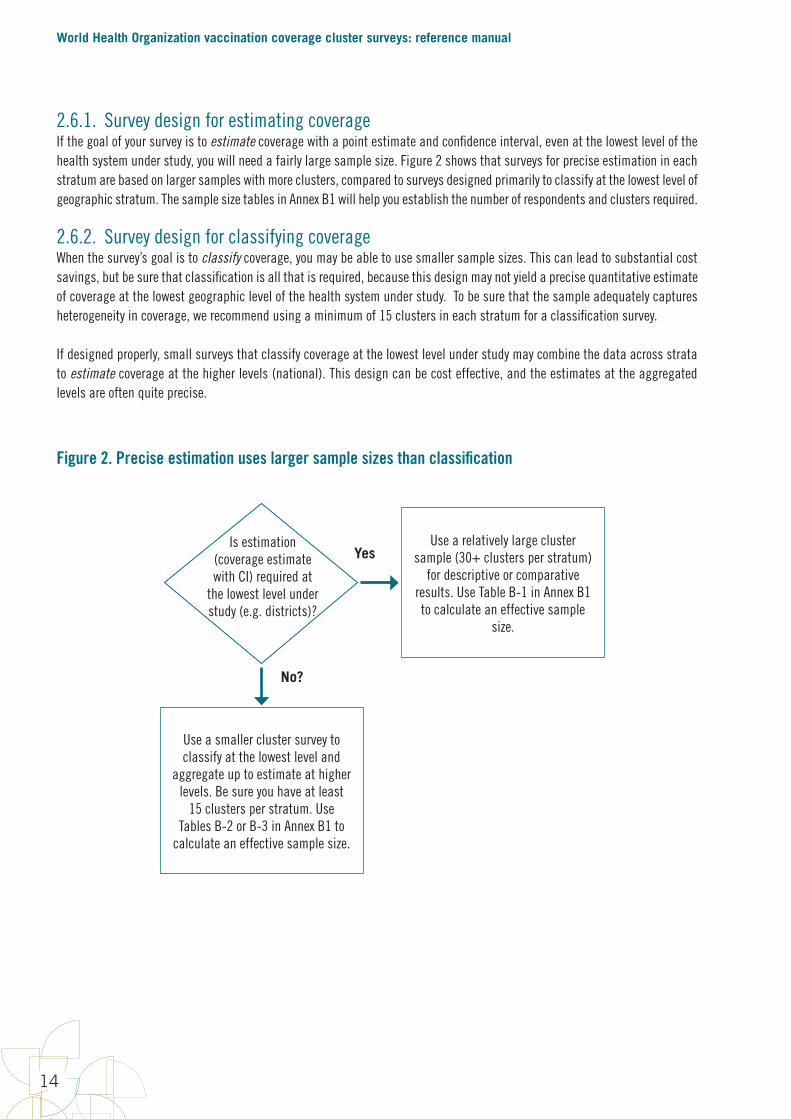
2.6.1. Survey design for estimating coverageIf the goal of your survey is to estimate coverage with a point estimate and confidence interval, even at the lowest level of the health system under study, you will need a fairly large sample size. Figure 2 shows that surveys for precise estimation in each stratum are based on larger samples with more clusters, compared to surveys designed primarily to classify at the lowest level of geographic stratum. The sample size tables in Annex B1 will help you establish the number of respondents and clusters required.
2.6.2. Survey design for classifying coverageWhen the survey’s goal is to classify coverage, you may be able to use smaller sample sizes. This can lead to substantial cost savings, but be sure that classification is all that is required, because this design may not yield a precise quantitative estimate of coverage at the lowest geographic level of the health system under study. To be sure that the sample adequately captures heterogeneity in coverage, we recommend using a minimum of 15 clusters in each stratum for a classification survey.
If designed properly, small surveys that classify coverage at the lowest level under study may combine the data across strata to estimate coverage at the higher levels (national). This design can be cost effective, and the estimates at the aggregated levels are often quite precise.
Figure 2. Precise estimation uses larger sample sizes than classification
Use a smaller cluster survey to classify at the lowest level and
aggregate up to estimate at higher levels. Be sure you have at least
15 clusters per stratum. Use Tables B-2 or B-3 in Annex B1 to
calculate an effective sample size.
Is estimation (coverage estimate with CI) required at
the lowest level under study (e.g. districts)?
No?
YesUse a relatively large cluster
sample (30+ clusters per stratum) for descriptive or comparative
results. Use Table B-1 in Annex B1 to calculate an effective sample
size.
2 Design the sample structure of the survey
15
2.7. Calculate the required sample sizeTo budget the survey accurately, you must calculate a sample size that will yield a dataset that meets the inferential goals. Annexes B1, B2, and B3 describe the parameters needed to calculate sample sizes. Work with the annexes or a sampling statistician to select a sample size (number of clusters and target number of respondents per cluster).
Box 1. Oversampling
If you plan to report precise survey results in several demographic subgroups, you must ensure that there are a sufficient number of respondents in each group. When a subgroup is comparatively small in the population, it is sometimes necessary to oversample members of that group, to purposefully interview more members of that group than might have appeared randomly in the sample. The respondents are still selected in a random fashion so their results are representative of the subgroup population. But the sampling plan takes specific measures to draw more respondents from areas where that subgroup lives. The precision of subgroup coverage estimates is determined by the subgroup sample size. When a survey oversamples some groups, their survey weights are specifically adjusted so their responses represent the appropriate proportion in calculations that combine subgroups. If it is important to obtain precise coverage estimates for demographic subgroups in your survey, work with a statistician to develop an appropriate sampling plan.
2.7.1. Sample size for estimating, classifying, or comparing coverageFor surveys of several non-overlapping geographical areas such as provinces or districts, where coverage will be assessed in each stratum, it is traditional to conduct what is essentially a separate survey in each stratum. The stratum-level results are often combined to estimate an aggregated coverage figure. For example, the steering group may wish to estimate coverage in each province in a country to within ± 5%, and also to combine the provincial figures to obtain a national coverage estimate with even more precision. See section 2.13 (near the end of this chapter) for specific advice regarding surveys conducted in several geographic areas at once.
Whether the goal is estimation of coverage with a confidence interval, or classification of coverage with respect to a threshold, a certain number of households must be visited to yield enough eligible, cooperative respondents to meet the survey’s inferential goals. This number is calculated by identifying a set of five numbers to multiply together: A x B x C x D x E. These parameters are described below, with additional details in Annexes B1, B2, and B3.
A. Identify the number of strata in which you will repeat the survey.
B. Use a table or equation to identify the base sample size per stratum (the effective sample size) – this is the sample size that would be needed with a simple random sample.
C. Use a table or equation to identify the likely design effect (DEFF), which is a multiplier required because this is a cluster survey and vaccination status is likely to be spatially correlated. Earlier survey guidelines have assumed a design effect of 2 when you lack a recent estimate from a similar survey in your country. Annex B1 shows how to estimate design effect using Table C; it suggests being conservative and selecting a higher value to make it likely to meet the inferential goals in strata where coverage varies substantially from area to area and cluster to cluster.

World Health Organization vaccination coverage cluster surveys: reference manual
16
D. Estimate the average number of households you will need to visit to find an eligible respondent. This will depend on the demographics of the survey target population as well as the birth rate and average household size in the country. It may vary between different regions or between rural and urban areas. In areas with disruption or seasonal mobility, this parameter might take into account the likelihood of abandoned or uninhabited households.
E. Use a table to identify a multiplier that accounts for expected non-response due to persons not being at home after at least two revisits, or eligible persons who refuse to participate.
For classifying coverage, there are additional parameters relating to the thresholds being examined (for example, probably below 90% or probably above 80%) and the probability of classification errors. Annex B2 describes each of these parameters.
Similar calculations are used to calculate sample sizes for comparing coverage, for example, to compare provinces over time, or HPV coverage among girls who do and do not attend school. For surveys comparing coverage, you will also need to specify the parameters for power and statistical significance.
Use Annexes B1, B2, and B3 to guide your selection of figures to multiply together. The next section discusses some of the common parameters used to calculate the sample size required to meet the survey’s inferential goals.
2.7.2. Common parameters for sample size calculationsThe calculations for each inferential goal require certain parameters. Gather these numbers, or estimate them, before you do the calculations. This section briefly describes the main parameters; additional definitions and details are in Annex A and Annexes B1, B2, and B3.
• Target population size: If the sample size turns out to be >10% of the target population then it will be worthwhile to apply a finite population correction to the sample size calculation and to the estimation equations. The details are not described here. Contact a sampling statistician for assistance.
• Anticipated vaccination coverage (p): The steering group will often have an idea of what coverage levels the survey will find, and those expectations can affect sample size. For a fixed level of precision or statistical power, larger sample sizes are required if the expected coverage is near 50%, while smaller sample sizes will suffice if the coverage is expected to be near 0% or 100%. This parameter may vary for different strata if the steering committee has sufficient information about the expected coverage in each stratum.
• Intracluster correlation coefficient (ICC): This is a measure of correlation of responses within clusters. This number affects the design effect (DEFF) and therefore affects the sample size calculation. Usually, you will not know this number in the planning stage, so you can use an observed figure from a recent survey in the study area. Alternately, you can use a conservative value that is slightly larger than what is likely to be observed in the field, to increase the likelihood that the results will have acceptable precision. Annex B1 gives some guidance on selecting ICC values.
• Confidence level (): This is usually 5%. The confidence intervals for estimation will be (100-) %, or usually 95%.
• Confidence interval (CI) half width: This measures the precision of a coverage estimate. If the (100-) % CI should be no wider than ± 5% (for example, CI = (52%, 62%)), this value will be 5%. The more precise the estimate, the narrower the CI will be, and a larger sample will be required. If less precision is acceptable, the CI will be wider and the required sample size will be smaller.5
5 Coverage figures are proportions, and the confidence interval (CI) for a proportion is essentially symmetric when the proportion is near 50%, but it is skewed if the proportion is near 0% or 100%. In this document, the sample sizes are designed so both sides of the CI are smaller than the precision target. That is, if you select a sample size to yield ± 5% precision, both the shorter and the longer sides of the CI should be ≤ 5%.

2 Design the sample structure of the survey
17
• Target number of respondents per cluster (m): This parameter is usually selected to fall between 5 and 15, and is based on the number of households a data collection team can visit in a day as well as the total number of target respondents expected in an average size cluster, assuming that all eligible respondents in those households visited are interviewed. We call this figure a target because we cannot know precisely how many eligible respondents will be found in each cluster. The number of completed questionnaires will vary from cluster to cluster, and the average number of eligible respondents per cluster will hopefully be ≥ m.
• Target number of clusters per stratum: The total sample size divided by m yields the target number of clusters per stratum. This number is fixed at the time the sample size is selected, and the clusters are selected randomly.
• Parameters relating to the statistical power of the test and the probability of errors. Annex B3 describes each of these parameters.
The next section provides a few examples of how to set these parameters.
Box 2. How much precision do you need?
After you carefully conduct a survey and estimate coverage and a 2-sided 95% confidence interval, imagine for a moment that you could request a visit from a helpful magical genie who will tell you the true proportion of children in the target population who have been vaccinated. Lucky you! She appears and tells you that the true coverage value is at the highest limit of the 2-sided confidence interval. You thank the genie … she disappears … and you prepare to act upon the coverage result. Imagine further that the embarrassed genie returns unexpectedly and confesses to a clerical error—the true coverage figure is not at the highest limit, but is actually at the very lowest limit of the 2-sided confidence interval. She begs your pardon and disappears again. What would you do? Would this new information change your plans for action?
If you would take the same action now that you know coverage is at the lower limit that you would have taken if coverage were at the upper limit, then the 2-sided confidence interval is precise enough for your purposes. But if you would take different actions depending on whether true coverage is at the lower or the upper limit, then we might say that the estimate is not precise enough. You need more precision.
2.7.3. Examples of calculating a sample size
Example 1: National level coverage only
If the steering group wishes to estimate national-level coverage with confidence intervals no wider than ± 10% when coverage is at 50%, then the tables in Annex B1 indicate that the numbers for A x B x C x D x E should be as follows:
A. Number of strata = 1 (national estimate only)
B. Effective sample size = 103 (Annex B1, Table B-1)
C. Assume we will collect data from an average of m=7 respondents per cluster and assume an intracluster correlation coefficient of 1/3, so the design effect will be 3. (Annex B1, Table C)6
D. Assume that an eligible child will be found in an average of 20% of the homes visited, based on the estimated number of households with children in the target age, so we must visit an average of 5 homes per eligible child.
E. Assume that 10% of families with eligible children will either not be at home when the survey team visits, or will refuse to participate in the survey, so we inflate the sample size by 11% to account for likely non-response. (Annex B1, Table E)
6 In this example we are using a conservative value of ICC and temporarily ignoring any extra DEFF that will result from unequal weights. If we have results from an earlier similar survey, we could also calculate the unequal weighting term of DEFF that is described in Annex B1.

World Health Organization vaccination coverage cluster surveys: reference manual
18
These values can be combined to calculate several quantities that are important for planning and budgeting purposes:
1. Estimated total target respondents with completed questionnaires: target = A x B x C = (1)(103)(3) = 309. The actual number will vary because different clusters will yield different numbers of eligible respondents.
2. Total households to visit to yield approximately 309 completed questionnaires: (A x B x C) x D x E = (309)(5)(1.11) = 1,715
3. Number of clusters
23
2.7.3. Examples of calculating a sample size Example1:Nationallevelcoverageonly
Ifthesteeringgroupwishestoestimatenational-levelcoveragewithconfidenceintervalsnowiderthan±10%whencoverageisat50%,thenthetablesinAnnexB1indicatethatthenumbersforAxBxCxDxEshouldbeasfollows:
A. Numberofstrata=1(nationalestimateonly)B. Effectivesamplesize=103(AnnexB1,TableB-1)C. Assumewewillcollectdatafromanaverageofm=7respondentsperclusterandassumean
intraclustercorrelationcoefficientof1/3,sothedesigneffectwillbe3.(AnnexB1,TableC)D. Assumethataneligiblechildwillbefoundinanaverageof20%ofthehomesvisited,basedon
theestimatednumberofhouseholdswithchildreninthetargetage,sowemustvisitanaverageof5homespereligiblechild.
E. Assumethat10%offamilieswitheligiblechildrenwilleithernotbeathomewhenthesurveyteamvisits,orwillrefusetoparticipateinthesurvey,soweinflatethesamplesizeby11%toaccountforlikelynon-response.(AnnexB1,TableE)
Thesevaluescanbecombinedtocalculateseveralquantitiesthatareimportantforplanningandbudgetingpurposes:
1. Estimatedtotaltargetrespondentswithcompletedquestionnaires:target=AxBxC=(1)(103)(3)=309.Theactualnumberwillvarybecausedifferentclusterswillyielddifferentnumbersofeligiblerespondents.
2. Totalhouseholdstovisittoyieldapproximately309completedquestionnaires:(AxBxC)xDxE=(309)(5)(1.11)=1,715
3. Numberofclusters=!#$%
=&'()=44.1.Roundupto45.
4. Numberofhouseholdstovisitpercluster=DxExm=(5)(1.11)(7)=38.85.Roundupto40.
Inthisexample,thesurveycallsfor45clusters(thatis,censusenumerationareasorEAs)—toberandomlyselectedacrossthecountry.IfEAsarelikelytoholdsubstantiallymorethan40households,thentheEAcanbedivided(usingdetailedmaps)intosegmentsthateachholdabout40householdsandasinglesegmentcanberandomlyselected(seeAnnexE).
Thisselectionisdonebeforethedatacollectorsgotothefield.Theteamplanningthesurveylogisticswilleitherusequalitysatellitemapsorwillmakeaplanningtriptoeachcluster.Ineithercase,theywilldrawanexcellentmapoftheclusteranditsboundaries.Afterselectingonerandomsegmenttheywillprepareamapforthefielddatacollectorstouse,showingtheboundariesoftheselectedsegmentveryclearly.Fielddatacollectorslatervisittheclustersandvisiteveryhouseholdinsidethecluster(orsegment)boundaries,takingdatafromalleligiblerespondents.Thenumberofcompletedinterviewsperclusterwillvarybecausetheteamisnotdoingaquotasamplebutinsteadinterviewingeveryeligiblerespondentinthepre-selectedsegment.Onaverage,thesurveyshouldyieldaboutsevencompletedsurveyspercluster.Plannerscandecidewhetherateamcandoalltheworkinaclusterinasingleday,orwhetheritismorerealistictoplantwodaysofworkpercluster,accountingfortheneed
44.1. Round up to 45.
4. Number of households to visit per cluster = D x E x m = (5)(1.11)(7) = 38.85. Round up to 40.
In this example, the survey calls for 45 clusters (that is, census enumeration areas or EAs)—to be randomly selected across the country. If EAs are likely to hold substantially more than 40 households, then the EA can be divided (using detailed maps) into segments that each hold about 40 households and a single segment can be randomly selected (see Annex E).
This selection is done before the data collectors go to the field. The team planning the survey logistics will either use quality satellite maps or will make a planning trip to each cluster. In either case, they will draw an excellent map of the cluster and its boundaries. After selecting one random segment they will prepare a map for the field data collectors to use, showing the boundaries of the selected segment very clearly. Field data collectors later visit the clusters and visit every household inside the cluster (or segment) boundaries, taking data from all eligible respondents. The number of completed interviews per cluster will vary because the team is not doing a quota sample but instead interviewing every eligible respondent in the pre-selected segment. On average, the survey should yield about seven completed surveys per cluster. Planners can decide whether a team can do all the work in a cluster in a single day, or whether it is more realistic to plan two days of work per cluster, accounting for the need to revisit households where no one is at home during the first interview attempt. The planners can also decide how many people make up a data collection team and how many teams one supervisor can effectively serve. These factors all affect the estimated budget for the survey.
Example 2: National and provincial coverage
Now assume that the steering group wishes to estimate routine vaccination coverage in each province as well as at the national level. In a country with five provinces, this essentially involves conducting five separate surveys, and then combining the results in a weighted fashion to estimate national level coverage. Suppose the steering group wishes to estimate coverage in each province with confidence intervals that are no wider than ± 5% when coverage is at 50% in each province. The tables in Annex B1 yield the following:
A. Number of strata = 5 (one survey in each province)
B. Effective sample size = 401 (Annex B1, Table B-1)
C. Assume we will collect data from an average of m=7 respondents per cluster, and assume an intracluster correlation coefficient of 1/3, so the design effect will be 3. (Annex B1, Table C)7
D. Assume that an eligible child will be found in an average of 20% of the homes visited, so we must visit an average of 5 homes per eligible child.
E. Assume that 10% of families with eligible children will either not be at home when the survey team visits or will refuse to participate in the survey, so inflate the sample size by 11% to account for likely non-response. (Annex B1, Table E)
These values can be combined to calculate several quantities that are important for planning and budgeting purposes:
7 As in the earlier example we temporarily ignore the term in the DEFF equation that accounts for unequal weights. Before finalizing the sample size, we should consider inflating DEFF based on what we can anticipate about the weights, as described in Annex B1.
2 Design the sample structure of the survey
19
1. Total target respondents with completed questionnaires: target = A x B x C = (5)(401)(3) = 6,015. The actual number will vary because different clusters will yield different numbers of eligible respondents.
2. Total households to visit to yield an average of 6,015 completed questionnaires: (A x B x C) x D x E = (6,015)(5)(1.11) = 33,384
3. Target households to visit in each province: B x C x D x E = (401)(3)(5)(1.11) = 6,677
4. Number of clusters per stratum =
24
torevisithouseholdswherenooneisathomeduringthefirstinterviewattempt.Theplannerscanalsodecidehowmanypeoplemakeupadatacollectionteamandhowmanyteamsonesupervisorcaneffectivelyserve.Thesefactorsallaffecttheestimatedbudgetforthesurvey.
Example2:Nationalandprovincialcoverage
Nowassumethatthesteeringgroupwishestoestimateroutinevaccinationcoverageineachprovinceaswellasatthenationallevel.Inacountrywithfiveprovinces,thisessentiallyinvolvesconductingfiveseparatesurveys,andthencombiningtheresultsinaweightedfashiontoestimatenationallevelcoverage.Supposethesteeringgroupwishestoestimatecoverageineachprovincewithconfidenceintervalsthatarenowiderthan±5%whencoverageisat50%ineachprovince.ThetablesinAnnexB1yieldthefollowing:
A. Numberofstrata=5(onesurveyineachprovince)B. Effectivesamplesize=401(AnnexB1,TableB-1)C. Assumewewillcollectdatafromanaverageofm=7respondentspercluster,andassumean
intraclustercorrelationcoefficientof1/3,sothedesigneffectwillbe3.(AnnexB1,TableC)D. Assumethataneligiblechildwillbefoundinanaverageof20%ofthehomesvisited,sowe
mustvisitanaverageof5homespereligiblechild.E. Assumethat10%offamilieswitheligiblechildrenwilleithernotbeathomewhenthesurvey
teamvisitsorwillrefusetoparticipateinthesurvey,soinflatethesamplesizeby11%toaccountforlikelynon-response.(AnnexB1,TableE)
Thesevaluescanbecombinedtocalculateseveralquantitiesthatareimportantforplanningandbudgetingpurposes:
1. Totaltargetrespondentswithcompletedquestionnaires:target=AxBxC=(5)(401)(3)=6,015.Theactualnumberwillvarybecausedifferentclusterswillyielddifferentnumbersofeligiblerespondents.
2. Totalhouseholdstovisittoyieldanaverageof6,015completedquestionnaires:(AxBxC)xDxE=(6,015)(5)(1.11)=33,384
3. Targethouseholdstovisitineachprovince:BxCxDxE=(401)(3)(5)(1.11)=6,677
4. Numberofclustersperstratum=!#$%
= *'+ &)
=172
5. Numberofhouseholdstovisitpercluster=DxExm=(5)(1.11)(7)=38.85.Roundupto40.
6. Totalclustersinthesurvey=,#!#$%
= - *'+)(&)
=860
Inthisexample,172clusterswillberandomlyselectedperprovince.Ineachofthoseclusters,detailedmapswillbeusedtodecidehowandwhethertosegmenttheclustertoidentifyarandomlyselectedcontiguousgroupof40households.All40householdsperclusterwillbevisitedandfielddatacollectorswillcompleteaquestionnaireforeacheligiblerespondent.Thenumberofcompletedquestionnaireswillvarypercluster,buttheaverageshouldbenear7.Separateweightedcoveragefigureswillbecalculatedforeachprovince,andthenalltheresultsmaybecombinedinaweightedcalculationtoestimatenationallevelcoverage.Thenationalcoveragefigureswillbeextremelyprecise,havingacombinedeffectivesamplesizeof(401)(5)=2,005.
5. Number of households to visit per cluster = D x E x m = (5)(1.11)(7) = 38.85. Round up to 40.
6. Total clusters in the survey =
24
torevisithouseholdswherenooneisathomeduringthefirstinterviewattempt.Theplannerscanalsodecidehowmanypeoplemakeupadatacollectionteamandhowmanyteamsonesupervisorcaneffectivelyserve.Thesefactorsallaffecttheestimatedbudgetforthesurvey.
Example2:Nationalandprovincialcoverage
Nowassumethatthesteeringgroupwishestoestimateroutinevaccinationcoverageineachprovinceaswellasatthenationallevel.Inacountrywithfiveprovinces,thisessentiallyinvolvesconductingfiveseparatesurveys,andthencombiningtheresultsinaweightedfashiontoestimatenationallevelcoverage.Supposethesteeringgroupwishestoestimatecoverageineachprovincewithconfidenceintervalsthatarenowiderthan±5%whencoverageisat50%ineachprovince.ThetablesinAnnexB1yieldthefollowing:
A. Numberofstrata=5(onesurveyineachprovince)B. Effectivesamplesize=401(AnnexB1,TableB-1)C. Assumewewillcollectdatafromanaverageofm=7respondentspercluster,andassumean
intraclustercorrelationcoefficientof1/3,sothedesigneffectwillbe3.(AnnexB1,TableC)D. Assumethataneligiblechildwillbefoundinanaverageof20%ofthehomesvisited,sowe
mustvisitanaverageof5homespereligiblechild.E. Assumethat10%offamilieswitheligiblechildrenwilleithernotbeathomewhenthesurvey
teamvisitsorwillrefusetoparticipateinthesurvey,soinflatethesamplesizeby11%toaccountforlikelynon-response.(AnnexB1,TableE)
Thesevaluescanbecombinedtocalculateseveralquantitiesthatareimportantforplanningandbudgetingpurposes:
1. Totaltargetrespondentswithcompletedquestionnaires:target=AxBxC=(5)(401)(3)=6,015.Theactualnumberwillvarybecausedifferentclusterswillyielddifferentnumbersofeligiblerespondents.
2. Totalhouseholdstovisittoyieldanaverageof6,015completedquestionnaires:(AxBxC)xDxE=(6,015)(5)(1.11)=33,384
3. Targethouseholdstovisitineachprovince:BxCxDxE=(401)(3)(5)(1.11)=6,677
4. Numberofclustersperstratum=!#$%
= *'+ &)
=172
5. Numberofhouseholdstovisitpercluster=DxExm=(5)(1.11)(7)=38.85.Roundupto40.
6. Totalclustersinthesurvey=,#!#$%
= - *'+)(&)
=860
Inthisexample,172clusterswillberandomlyselectedperprovince.Ineachofthoseclusters,detailedmapswillbeusedtodecidehowandwhethertosegmenttheclustertoidentifyarandomlyselectedcontiguousgroupof40households.All40householdsperclusterwillbevisitedandfielddatacollectorswillcompleteaquestionnaireforeacheligiblerespondent.Thenumberofcompletedquestionnaireswillvarypercluster,buttheaverageshouldbenear7.Separateweightedcoveragefigureswillbecalculatedforeachprovince,andthenalltheresultsmaybecombinedinaweightedcalculationtoestimatenationallevelcoverage.Thenationalcoveragefigureswillbeextremelyprecise,havingacombinedeffectivesamplesizeof(401)(5)=2,005.
In this example, 172 clusters will be randomly selected per province. In each of those clusters, detailed maps will be used to decide how and whether to segment the cluster to identify a randomly selected contiguous group of 40 households. All 40 households per cluster will be visited and field data collectors will complete a questionnaire for each eligible respondent. The number of completed questionnaires will vary per cluster, but the average should be near 7. Separate weighted coverage figures will be calculated for each province, and then all the results may be combined in a weighted calculation to estimate national level coverage. The national coverage figures will be extremely precise, having a combined effective sample size of (401)(5) = 2,005.
Note that increasing precision from ± 10% in Example 1 to ± 5% in Example 2 increased the effective sample size from 103 to 401. It is costly to have an increased sample size to improve the precision. See Table B-2 in Annex B1 for additional detail on this point.
Example 3: Imprecise estimation for classification at the province level
In Example 2, it would be quite expensive to achieve an effective sample size of 401 per province. Upon reflection, the steering group may decide that they do not strictly need ± 5% precision everywhere, but rather they want to clarify which provinces have very high coverage, which ones have very low coverage, and which are likely to have coverage in between.
For example, if an important programmatic threshold for DTPCV3 is 80%, the steering group may wish to identify which provinces have coverage that is clearly higher than 80%, clearly lower than 80%, or likely to be near 80%. This is a classification goal; Tables B-2 and B-3 in Annex B1 are relevant here for calculating the effective sample size (parameter B).
This manual suggests using one-sided confidence bounds to classify coverage. Select a sample size for each stratum, conduct the survey, and calculate confidence bounds. The classification rules are as follows:
1. If the one-sided 95% lower confidence bound is above the threshold, classify coverage as being very likely to fall above the threshold.
2. If the one-sided 95% upper confidence bound is below the threshold, classify coverage as being very likely to fall below the threshold.
3. If the upper and lower one-sided bounds fall on either side of the threshold, one above and one below, conclude that the sample size was too small to classify the coverage as being above or below 80% with 95% confidence.
This last result might be disappointing: you have spent a substantial amount of money and effort to collect data just to find that the classification result is inconclusive. To avoid this situation, you would have to select a sample size large enough to yield conclusive results for your survey’s threshold. To classify which strata are likely to have coverage above or below 80%, the study designer selects a distance from the threshold, called delta, and uses Tables B-2 or B-3 to look up a sample size that will guarantee a suitably high probability that the one-sided confidence bound will fall on the correct side of the threshold.
World Health Organization vaccination coverage cluster surveys: reference manual
20
This affects the required sample size dramatically. If coverage in a stratum is very high (for example, 95%), then a survey with an effective sample size as low as 45 will yield a sample where the one-sided 95% lower confidence bound is very likely to fall above the important threshold of 80%. However, the closer you get to 80%, the bigger the effective sample size will need to be. If the true coverage is 85%, you will need an effective sample size of about 250. If the true coverage is 81%, you will need an effective sample size of nearly 10,000 respondents to draw a confident conclusion that coverage is above the 80% threshold!
This process of classification is illustrated graphically in Annex N and in Figure 10 in section 6.5.2. There are sample sizes in Annex B3 to help draw strong conclusions for delta values of 1%, 5%, 10%, and 15%. Smaller delta values require much larger sample sizes to yield conclusive classification results.
The important point in this example is that programmatically useful classification can sometimes be achieved using smaller sample sizes than needed for precise estimation if the study designer is willing to accept classification #3 above (sample size not large enough to classify with 95% confidence) when the true coverage is within delta points of the programmatic threshold. Although it can be disappointing to have inconclusive classification results in some strata, there are three features that make the results programmatically valuable:
1. The graphic portrayal of the coverage results, as illustrated in Annex N, will sometimes make it clear that coverage is very likely to fall above or below the threshold, even when a conclusion may not be assigned 95% confidence. In other words, if one of the one-sided bounds is quite near the threshold, you may be able to confidently classify coverage, albeit with a confidence level slightly lower than 95%.
2. You will interpret the inconclusive results in the context of strata with conclusive results, so if some strata are classified as above the threshold, some below, and some inconclusive, then you know where the inconclusive strata fall compared with the others.
3. Finally, if the sample uses nested strata, like sampling from all provinces in a nation, the results from conclusive and inconclusive strata alike will be aggregated together to estimate and classify coverage quite precisely at the national level.
Example 4: HPV coverage among 12-year-old girls
In this example the steering group is evaluating coverage with Human Papilloma Virus (HPV) vaccine among girls aged 12 in a single province. If the vaccine is administered through location-based methods, possibly at schools, then the survey might have several goals:
1. Estimate coverage among those most likely to benefit from the vaccine administration strategy – girls who are enrolled in school and regularly attend.
2. Estimate coverage among the overall population of girls who need the vaccine – girls who are a particular age (for example, 12), regardless of whether they attend school.
The first goal might evaluate the success of the delivery strategy while the second goal evaluates the likely population protection in a cohort defined by age.
If the inferential goal is to estimate coverage of 2 or more HPV doses among girls age 12 with precision no worse than ± 5% if coverage is 75%, then the tables in Annex B1 yield the following:
2 Design the sample structure of the survey
21
A. Number of strata = 1 (a single survey in a single province)
B. Effective sample size = 340 (Annex B1, Table B-1)
C. Assume we will collect data from an average of m=10 respondents per cluster and assume an intracluster correlation coefficient of 1/6, so the design effect will be 2.5. (Annex B1, Table C)8
D. Assume that an eligible child will be found in an average of 10% of the homes visited, so we must visit an average of 10 homes per eligible girl.
E. Assume that 10% of families with eligible children will either not be at home when the survey team visits or will refuse to participate in the survey, so inflate the sample size by 11% to account for likely non-response. (Annex B1, Table E)
These values can be combined to calculate several quantities that are important for planning and budgeting purposes:
1. Total target respondents with completed questionnaires: target = A x B x C = (1)(340)(2.5)= 850. The actual number will vary because different clusters will yield different numbers of eligible respondents.
2. Total households to visit to yield an average of 6,015 completed questionnaires: (A x B x C) x D x E = (850)(10)(1.11) = 9,435
3. Number of clusters =
27
D. Assumethataneligiblechildwillbefoundinanaverageof10%ofthehomesvisited,sowemustvisitanaverageof10homespereligiblegirl.
E. Assumethat10%offamilieswitheligiblechildrenwilleithernotbeathomewhenthesurveyteamvisitsorwillrefusetoparticipateinthesurvey,soinflatethesamplesizeby11%toaccountforlikelynon-response.(AnnexB1,TableE)
Thesevaluescanbecombinedtocalculateseveralquantitiesthatareimportantforplanningandbudgetingpurposes:
1. Totaltargetrespondentswithcompletedquestionnaires:target=AxBxC=(1)(340)(2.5)=850.Theactualnumberwillvarybecausedifferentclusterswillyielddifferentnumbersofeligiblerespondents.
2. Totalhouseholdstovisittoyieldanaverageof6,015completedquestionnaires:(AxBxC)xDxE=(850)(10)(1.11)=9,435
3. Numberofclusters=!#$%
= &*' 0.-+'
=85
4. Numberofhouseholdstovisitpercluster=DxExm=(10)(1.11)(10)=111
Inthisexample,85clusterswillberandomlyselectedintheprovince.Ineachcluster,detailedmapswillbeusedtodecidehowandwhethertosegmenttheclustertoidentifyarandomlyselectedcontiguousgroupof111households.All111householdsperclusterwillbevisited,anddatacollectorswillcompleteaquestionnaireforeachgirlwhois12yearsold.Thenumberofcompletedquestionnaireswillvarypercluster,buttheaverageshouldbenearten.Iftheestimatedcoverageisnotlowerthan75%andiftheICCisnothigherthantheassumed1/6,thentheconfidenceintervalshouldbenowiderthan±5%.
Noteagainherethattherelativelylargesamplesizeisdrivenbytherequirementfornarrowprecision.Ifthesteeringcommitteewerewillingtoacceptprecisionof±7%,thenTableB-1indicatesthattheeffectivesamplesizewoulddropfrom340to182andthenumberofclusterswoulddropfrom85to46.
Ifthevaccinedeliverystrategywasschool-basedandifschoolattendancewasnot100%among12-year-oldgirls,thenaportionofthesampledgirlswouldbeunschooledandlesslikelytohavebeenvaccinated.Sotheestimatedcoverageamongthesurveypopulationwouldbeamixofthecoverageamongschoolgirlsandcoverageamongunschooledgirls.Thiswouldtendtoyieldalowercoverageestimate,whichmightbeappropriateforevaluatingpopulationlevelprotection,butwouldlikelyunderestimatecoverageamongschoolgirlsonly.Toguaranteeahighprecisionestimateofcoverageamongschoolgirlsitwouldbenecessarytoeitherrestrictthesurveysampletoschoolgirls,ortooversampleschoolgirls.Iftheseapproacheswerepursuedinahouseholdsurveythenitwouldlikelybenecessarytovisitmorethan10householdstofindeacheligiblerespondentandsotheplanningwouldneedtoaccountforadditionaleffort.
2.8. Draft an analysis plan, table shells and report figures Atthisstageintheplanningprocess,itishelpfultodraftananalysisplanandlayouttableshellsforthefinalsurveyreport.Thiswillhelpyoubudgetrealisticallyfortheanalysisportionoftheproject,andwill
4. Number of households to visit per cluster = D x E x m = (10)(1.11)(10) = 111
In this example, 85 clusters will be randomly selected in the province. In each cluster, detailed maps will be used to decide how and whether to segment the cluster to identify a randomly selected contiguous group of 111 households. All 111 households per cluster will be visited, and data collectors will complete a questionnaire for each girl who is 12 years old. The number of completed questionnaires will vary per cluster, but the average should be near ten. If the estimated coverage is not lower than 75% and if the ICC is not higher than the assumed 1/6, then the confidence interval should be no wider than ± 5%.
Note again here that the relatively large sample size is driven by the requirement for narrow precision. If the steering committee were willing to accept precision of ± 7%, then Table B-1 indicates that the effective sample size would drop from 340 to 182 and the number of clusters would drop from 85 to 46.
If the vaccine delivery strategy was school-based and if school attendance was not 100% among 12-year-old girls, then a portion of the sampled girls would be unschooled and less likely to have been vaccinated. So the estimated coverage among the survey population would be a mix of the coverage among schoolgirls and coverage among unschooled girls. This would tend to yield a lower coverage estimate, which might be appropriate for evaluating population level protection, but would likely underestimate coverage among schoolgirls only. To guarantee a high precision estimate of coverage among schoolgirls it would be necessary to either restrict the survey sample to schoolgirls, or to oversample schoolgirls. If these approaches were pursued in a household survey then it would likely be necessary to visit more than 10 households to find each eligible respondent and so the planning would need to account for additional effort.
8 This example ignores the extra inflation to DEFF that occurs because of unequal weights.
World Health Organization vaccination coverage cluster surveys: reference manual
22
2.8. Draft an analysis plan, table shells and report figuresAt this stage in the planning process, it is helpful to draft an analysis plan and lay out table shells for the final survey report. This will help you budget realistically for the analysis portion of the project, and will also confirm whether the survey design will meet the programmatic goals of the survey stakeholders. See Chapter 6 and the Vaccination Coverage Quality Indicators (VCQI) documentation for examples on the WHO website.
2.9. Budget for the survey and estimate the timelineNext, create a budget for the survey design you’ve selected. As you budget money and time, consider all aspects listed in this manual. Consult Table 2 for a list of activities and items to include in the budget. In addition to budgeting the monetary cost of the survey, make an estimate of the project timeline, accounting realistically for likely delays. Remember that your top priority is to ensure high data quality. To do this, you should have only as many field teams as can realistically be well supervised. It is better to use a small number of field teams and take longer to implement the survey than to have so many field teams that their training and supervision suffers, and data quality is compromised.
In addition to fixed costs, the cost of cluster surveys is proportional to the number of strata, the number of clusters per stratum, and the total number of respondents. Be sure to include all items with a cost that depends upon the questions, goals, sampling design, or sample size. See the DHS and MICS budget templates at http://dhsprogram.com/publications/publication-dhsm10-dhs-questionnaires-and-manuals.cfm and http://mics.unicef.org/tools for examples.
The timetable should likewise be adjusted according to the specific needs of the survey and, especially, the local administrative procedures required. Often, it takes additional time to access funds, choose a contractor to do the survey (if one is used) and gain ethical clearance from the relevant organizations.
For post-SIA surveys, it is best to conduct fieldwork very soon after the campaign in order to have a chance of seeing finger marks indicating vaccination or retrieving any SIA-specific cards that were given to caretakers. Thus, it is important to prepare for the survey well in advance, ideally at the same time you prepare for SIA implementation. The training and fieldwork for a post-SIA survey can be shorter than the timeline in Table 2 suggests, if data are only needed at the national level and only vaccines administered in the SIA are assessed. If the steering group requests data at the province or district level, and especially if they also request these data on all routine vaccinations, the survey becomes much larger, and it will probably not be completed quickly after the SIA ends. In order to ensure high-quality data, if results are needed quickly, it is better to compromise on the goals of the survey than to add too many field teams.
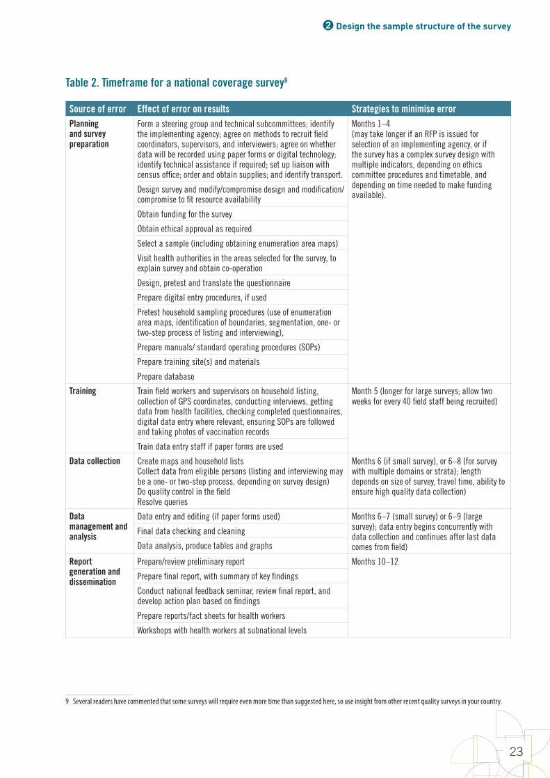
2 Design the sample structure of the survey
23
Table 2. Timeframe for a national coverage survey9
Source of error Effect of error on results Strategies to minimise errorPlanning and survey preparation
Form a steering group and technical subcommittees; identify the implementing agency; agree on methods to recruit field coordinators, supervisors, and interviewers; agree on whether data will be recorded using paper forms or digital technology; identify technical assistance if required; set up liaison with census office; order and obtain supplies; and identify transport.
Months 1–4 (may take longer if an RFP is issued for selection of an implementing agency, or if the survey has a complex survey design with multiple indicators, depending on ethics committee procedures and timetable, and depending on time needed to make funding available).
Design survey and modify/compromise design and modification/compromise to fit resource availability
Obtain funding for the survey
Obtain ethical approval as required
Select a sample (including obtaining enumeration area maps)
Visit health authorities in the areas selected for the survey, to explain survey and obtain co-operation
Design, pretest and translate the questionnaire
Prepare digital entry procedures, if used
Pretest household sampling procedures (use of enumeration area maps, identification of boundaries, segmentation, one- or two-step process of listing and interviewing),
Prepare manuals/ standard operating procedures (SOPs)
Prepare training site(s) and materials
Prepare database
Training Train field workers and supervisors on household listing, collection of GPS coordinates, conducting interviews, getting data from health facilities, checking completed questionnaires, digital data entry where relevant, ensuring SOPs are followed and taking photos of vaccination records
Month 5 (longer for large surveys; allow two weeks for every 40 field staff being recruited)
Train data entry staff if paper forms are used
Data collection Create maps and household listsCollect data from eligible persons (listing and interviewing may be a one- or two-step process, depending on survey design)Do quality control in the fieldResolve queries
Months 6 (if small survey), or 6–8 (for survey with multiple domains or strata); length depends on size of survey, travel time, ability to ensure high quality data collection)
Data management and analysis
Data entry and editing (if paper forms used) Months 6–7 (small survey) or 6–9 (large survey); data entry begins concurrently with data collection and continues after last data comes from field)
Final data checking and cleaning
Data analysis, produce tables and graphs
Report generation and dissemination
Prepare/review preliminary report Months 10–12
Prepare final report, with summary of key findings
Conduct national feedback seminar, review final report, and develop action plan based on findings
Prepare reports/fact sheets for health workers
Workshops with health workers at subnational levels
9 Several readers have commented that some surveys will require even more time than suggested here, so use insight from other recent quality surveys in your country.
World Health Organization vaccination coverage cluster surveys: reference manual
24
2.10. Evaluate affordability and timelinessIf the proposed design is affordable and the results are likely to be available in the timeframe needed, you can begin to do more specific planning, as described in Chapter 3.
If the design is not affordable or if it would take too long, either appropriate more money for the survey or modify some combination of questions, strata, and inferential goals to find a lower-cost design that still addresses the steering group’s primary questions, with an acceptable level of uncertainty and in an acceptable timeframe. See below for examples of compromise strategies.
If the designs that are affordable do not adequately address the primary programmatic questions, the steering group should seriously consider not doing a survey at this time, and instead use other methods to assess and strengthen vaccination services. See Cutts, Claquin, Danovaro-Holliday & Rhoda, 2016.
If it is not possible to appropriate more money to conduct a large survey that meets the initial goals of the survey steering group, but some sort of survey is still desirable, the design team must compromise on one or more parameters to find a less expensive survey that still yields helpful results. These parameters may be varied to reduce the cost of the survey.
1. Adjust the number of geographic strata in which conclusions will be reported. If the steering group wants results in all districts but the cost is too high, it might be affordable to do a survey in each province instead.
2. Adjust the survey goals in different strata. For example, you might estimate SIA coverage at the province level but assess routine vaccination coverage at the national level only. Since the target age group for SIA coverage is much wider than for routine immunization, sample sizes are reached by visiting a smaller number of households for SIA than for RI coverage.
3. Adjust the desired precision of the coverage estimates in each stratum. Accepting additional uncertainty will decrease the effective sample size.
4. Classify rather than estimate coverage at the lowest geographic hierarchy level. Rather than calculating a narrow confidence interval in each district, it may often suffice to use a smaller sample to classify coverage in each district, and aggregate data across districts to estimate coverage precisely at the province and national levels. The smaller sample will identify districts that are doing very poorly and those that are doing very well. There is likely to be a middle category of districts that are not clearly doing either poorly or well. In order to identify their current coverage precisely, a larger survey would be needed, but at least the small survey identifies that they are neither at the top nor the bottom of the performance continuum. When three or more strata are aggregated up to the next level of hierarchy, the confidence intervals typically become substantially more narrow and informative.
For example, assume a country has 10 provinces, each having between 15 and 25 districts, for a national total of 203 districts. The steering group may initially wish to estimate coverage in all districts with ± 5% precision. Average national coverage of DTPCV3 is thought to be 85%, varying from 55% to 95% between districts. To estimate coverage to ± 5% when it is only 55%, using a design effect of 4 requires 1,600 completed interviews.10 At 10 completed questionnaires per cluster, this would require 160 clusters per district. Repeating this in 203 districts would require visiting 32,480 clusters and collecting data from 324,800 respondents! This is prohibitively expensive, and would take a very long time to implement while ensuring high quality. Below are options for revising the survey goals.
1. Estimate coverage at national level and in a small number of key districts (such as those thought to have particularly poor administrative data, those where major recent programmatic or demographic changes occurred, or major metropolitan areas).
10 The WHO 2005 reference manual always used a design effect of 2. In practice, the design effects observed in vaccination coverage surveys have often exceeded 2, so this manual recommends a more conservative value of 3 if there are 7 respondents per cluster, or 4 if there are 10 respondents per cluster.

2 Design the sample structure of the survey
25
2. Classify coverage in all districts and aggregate data to estimate coverage at provincial and national levels. Classification might be achieved using 15 or 20 clusters per district. This would require a total of (203 x 15) = 3,045 clusters, covering all districts of the country. Although the total sample size will be smaller than when coverage is estimated in all districts, there are still important logistical considerations for getting well trained and supervised teams to this many clusters.
3. Estimate coverage precisely at only the provincial and national levels, using, for example, 160 clusters per province. This requires a total of (10 x 160) = 1,600 clusters, which may not necessarily include all districts if some districts have very small populations. The precision of coverage estimates at the provincial level could also be varied, to determine the effect on budget and time.
4. Estimate coverage imprecisely at the provincial level, for example, using 30 clusters per province and aggregating to estimate coverage at the national level. This means visiting only (10 x 30) = 300 clusters – a substantially smaller sample size than the other options. It will yield, however, imprecise estimates at the provincial level. This will be useful for identifying (classifying) provinces that are clearly low or clearly high, but not useful for making fine distinctions between provinces whose coverage levels are nearly equal.
The options here fit a wide range of budgets, ranging from 32,480 clusters down to 300 clusters. The larger options yield precise district level estimates and the smallest option yields precise estimates only at the national level, while providing some insight into which provinces are performing best or worst.
2.11. Implications of adding routine immunization questions to a post-SIA surveyIt is increasingly common for survey stakeholders to consider adding questions about routine immunization (RI) to a survey designed to evaluate SIA coverage. Planners may reason that substantial resources are already being devoted to planning and conducting a nationally representative survey, and believe those resources should be leveraged to assess the performance of the RI services while the survey staff are already in the field to collect data. It seems reasonable, but an RI survey can require a much larger field effort than a post-SIA survey does. Sorting out what is best in each situation will require careful consideration, to strike a balance between a lean and timely SIA coverage estimate and a precise, geographically specific, multi-vaccine assessment of RI services.
Whether it is feasible and affordable to bundle RI questions with an SIA survey will depend on the inferential goals of both surveys. The best time to work through these issues is long before the actual SIA begins.
These are some considerations that may substantially expand the resources required when adding RI questions to an SIA survey:
• The window of age-eligibility is very small for RI surveys (usually a one- or two-year window) compared with that for an SIA (often a 14-year window), so the survey staff must visit more households just to find an eligible respondent. If precise RI coverage estimates are desired, the number of homes to visit in each cluster will be multiplied by a large factor – possibly five or more. This is a substantial increase in cost and logistical complexity.
• The standard RI questionnaire takes much longer to complete than a post-SIA interview, so field staff will be able to complete substantially fewer interviews per day.
• RI coverage figures for important vaccines are often much lower than SIA coverage achieved, thus requiring a larger sample size to achieve the target precision.
• The intracluster correlation coefficient (ICC), which drives the design effect, will be substantially higher for RI vaccines than for that observed in a well-run SIA with consistently high coverage, so the RI design effect will increase the required sample size for precise estimation.
• It is a best practice in RI surveys to visit health facilities and obtain vaccination dates from EPI registers if the child’s caretaker cannot furnish a home-based record. This also represents a substantial commitment of time and resources.
World Health Organization vaccination coverage cluster surveys: reference manual
26
• Finally, stakeholders may wish to estimate RI coverage in many more, smaller strata (such as health districts) than the people evaluating SIA coverage do. As described above, the overall sample size is proportional to the number of strata where you will report results, so this can increase the survey sample size.
If the idea to add an RI component occurs late in the SIA survey planning process, the extra planning and resources required could easily postpone the survey fieldwork for several months. A long delay will likely degrade the quality of SIA coverage responses and estimates, by increasing recall bias.
But if the goals of the SIA campaign are for precise estimation and the goals of the RI survey are less precise, and if the geographic or administrative focus is similar for both surveys, then it may be possible to add an RI component without much extra effort or delays. For example, it may be relatively easy to add an RI component if the RI survey requires results at a higher level of hierarchy (province level) than the SIA survey (district level). The key is to discuss it early, estimate the sample size and timeline realistically, and explore whether there is a design that does indeed leverage the SIA survey resources without compromising its goals.
2.12. Designing for multiple outcomesSample size calculations are most straightforward when the survey steering group identifies a single primary goal to size the survey. When agreement cannot be reached on a primary goal, it is possible to do sample size calculations independently for two or more goals, and estimate a budget for the largest of the several sample sizes. If that design is affordable, it should be possible to meet all the goals. If it is not affordable, some sort of compromise will be necessary.
2.13. Designing for multiple geographic areasIf you are planning to assess coverage in more than one geographic or administrative area, it will be necessary to calculate the sample size required in each area to estimate the budget for the survey. In some cases the sample sizes may vary considerably from one stratum to another, especially if the fertility rates or expected coverage vary substantially. Strata with coverage near 50% will require larger samples to obtain a given level of precision (for example, ± 5%) than strata with coverage near 0% or 100%. A simple shortcut may be to calculate the required sample size that is likely to be largest, and conduct surveys of that size in each stratum. You may save some money and time, however, by calculating sample sizes for each stratum individually, based on what is known about each stratum’s sample size inputs.
For example, using Table B-1 in Annex B1, to estimate coverage with ± 5% precision requires an effective sample size of 401 if coverage is in the range of 50%–70%, but only requires an effective sample size of 216 if coverage is near 90%. Substantial savings are potentially available by doing a smaller survey in locations with higher coverage. Of course, if you knew the coverage before doing the survey, you would not need to do a survey at all, so it is usually a good idea to select a conservative sample size in case coverage is closer to 50% than was originally anticipated.
Similarly, if fertility rates vary substantially by urban/rural status or by ethnic group, then the number of households to visit per cluster may vary enough to achieve some important cost savings by customizing the calculation of number of households to visit by stratum.
2.14. Designing for multiple levels of administrative or geographic hierarchyCoverage surveys often assess coverage for several levels of a geographic or administrative hierarchy. The steering group may wish to estimate coverage within each province, and then aggregate results to estimate national coverage figures. In other situations coverage may be assessed at three levels. For example, the steering group may wish to identify all districts where SIA
2 Design the sample structure of the survey
27
coverage is very likely to be below 95% and aggregate district surveys to estimate coverage in each province, with a confidence interval no wider than ± 5%, and then aggregate provincial results up to a national coverage figure with a confidence interval that is even more narrow, such as ± 3%.
In these cases, identify the level in the hierarchy with the most important inferential goal, identify a design and sample size that will meet that goal, and check to see whether the goals at other levels will be met as well. It is often the lowest level of the hierarchy (that is, those with the smallest geographic or administrative extent) where the survey results will be used to drive actions. The goals at that level are often the most important, with precision at higher levels being of secondary importance. If a design meets the goals at one level, but does not meet the inferential goals at another level, you will likely need to increase the sample size to move closer to satisfying goals at all levels. Balance this option against the budget and time implications of conducting a larger survey.
The tools in this manual should help survey teams identify designs that will meet goals at the most important level. In situations that are not complicated, it may also help them assess whether a single design will meet goals at multiple levels. For more complex scenarios, it will be helpful to enlist help from a sampling statistician.
Example: Combining multiple outcomes and multiple levels of hierarchy
Consider a measles campaign coverage survey in a country with 60 health districts, nested within ten provinces. Possible inferential goals might be:
1. estimate campaign coverage nationally, without reporting subnational results (1 stratum);
2. estimate campaign coverage in each province and nationally (10 strata; number of clusters depends on desired precision);
3. classify coverage in each province and estimate national coverage precisely (10 strata; fewer clusters per province than in the previous design);
4. estimate coverage in each district, and aggregate for provincial and national results (60 strata; number of clusters depends on desired precision); or
5. classify coverage in each district, and aggregate for provincial and national results (60 strata; fewer clusters per district than in the previous design).
Assume the steering group selects option 5. They will conduct a separate survey in each of 60 districts, using 15 clusters each and a target number of 10 completed interviews per cluster. The target age range group for the campaign is 9 months to 14 years, so they expect to find a cooperative, eligible respondent in every second household they visit, on average. That means visiting 20 randomly selected households per cluster, or 300 per district, or 18,000 nationwide. The number of expected completed interviews is 10 per cluster, 150 per district, 900 per province, and 9,000 nationally. In comparison to the classic 30 x 7 design, this survey is somewhat smaller, at 15 x 10. But it is being conducted in every district, so the overall effort and sample size is very large.
Now consider adding an RI component to the survey. The reasoning is logical: since the post-campaign survey will be nationally representative and survey workers will visit 18,000 homes across the land, why not also estimate RI coverage at the same time? If the sample size is fixed and you can find one child aged 12–23 months with a cooperative caretaker in every five households visited, the expected number of RI respondents per cluster is four, the expected number per district is 60, the expected number per province is 360, and the expected number nationally is 3,600.
Adding the RI component has numerous implications for survey logistics, data collection, data management, analysis and reporting, and cost and schedule. Each cluster’s work will take longer because you are adding an average of four RI interviews per cluster. Four RI interviews could turn into eight interviews if you also ask about tetanus vaccinations among women who gave birth in the last year. The supervision, training and data collection will be more complicated than for a simple post-campaign survey. The additional complexity of conducting three simultaneous surveys (SIA, 12–23 months for RI, and 0–11 months for tetanus) may tempt the survey organizers to collect primary data using handheld electronic devices. Will they photograph
World Health Organization vaccination coverage cluster surveys: reference manual
28
vaccination cards? Visit health facilities in search of documented evidence of vaccination? In some cases, the steering group may decide that the added insight is worth the cost of adding the RI component.
Careful consideration should be given at this point to whether adding the RI component will delay the start of the fieldwork and possibly compromise the quality of campaign-related responses. Finger marks from the SIA campaign may no longer be visible by the time the survey begins, or caretakers may lose their campaign-issued vaccination cards and forget or become confused about which of their children were vaccinated in the campaign. Furthermore, in countries with important seasonal migration due to weather, agriculture, and availability of work, a delay will give people time to move; some who were vaccinated will leave and some who were not will return. The survey results will reflect a combination of campaign effectiveness and population movement, which may be challenging to interpret.
Another consideration is the precision of the RI coverage estimates. With such a small number of RI respondents per cluster, the design effect would likely be small (maybe 1.5), so the effective sample size per province would be 240. Table B-1 in Annex B1 indicates that this is sufficient to yield precision of ± 6% at the province level if RI coverage were 75%. The effective sample size in each district would be
35
10percluster,150perdistrict,900perprovince,and9,000nationally.Incomparisontotheclassic30x7design,thissurveyissomewhatsmaller,at15x10.Butitisbeingconductedineverydistrict,sotheoveralleffortandsamplesizeisverylarge.
NowconsideraddinganRIcomponenttothesurvey.Thereasoningislogical:sincethepost-campaignsurveywillbenationallyrepresentativeandsurveyworkerswillvisit18,000homesacrosstheland,whynotalsoestimateRIcoverageatthesametime?Ifthesamplesizeisfixedandyoucanfindonechildaged12–23monthswithacooperativecaretakerineveryfivehouseholdsvisited,theexpectednumberofRIrespondentsperclusterisfour,theexpectednumberperdistrictis60,theexpectednumberperprovinceis360,andtheexpectednumbernationallyis3,600.
AddingtheRIcomponenthasnumerousimplicationsforsurveylogistics,datacollection,datamanagement,analysisandreporting,andcostandschedule.Eachcluster’sworkwilltakelongerbecauseyouareaddinganaverageoffourRIinterviewspercluster.FourRIinterviewscouldturnintoeightinterviewsifyoualsoaskabouttetanusvaccinationsamongwomenwhogavebirthinthelastyear.Thesupervision,traininganddatacollectionwillbemorecomplicatedthanforasimplepost-campaignsurvey.Theadditionalcomplexityofconductingthreesimultaneoussurveys(SIA,12–23monthsforRI,and0–11monthsfortetanus)maytemptthesurveyorganizerstocollectprimarydatausinghandheldelectronicdevices.Willtheyphotographvaccinationcards?Visithealthfacilitiesinsearchofdocumentedevidenceofvaccination?Insomecases,thesteeringgroupmaydecidethattheaddedinsightisworththecostofaddingtheRIcomponent.
CarefulconsiderationshouldbegivenatthispointtowhetheraddingtheRIcomponentwilldelaythestartofthefieldworkandpossiblycompromisethequalityofcampaign-relatedresponses.FingermarksfromtheSIAcampaignmaynolongerbevisiblebythetimethesurveybegins,orcaretakersmaylosetheircampaign-issuedvaccinationcardsandforgetorbecomeconfusedaboutwhichoftheirchildrenwerevaccinatedinthecampaign.Furthermore,incountrieswithimportantseasonalmigrationduetoweather,agriculture,andavailabilityofwork,adelaywillgivepeopletimetomove;somewhowerevaccinatedwillleaveandsomewhowerenotwillreturn.Thesurveyresultswillreflectacombinationofcampaigneffectivenessandpopulationmovement,whichmaybechallengingtointerpret.
AnotherconsiderationistheprecisionoftheRIcoverageestimates.WithsuchasmallnumberofRIrespondentspercluster,thedesigneffectwouldlikelybesmall(maybe1.5),sotheeffectivesamplesizeperprovincewouldbe240.TableB-1inAnnexB1indicatesthatthisissufficienttoyieldprecisionof±
6%attheprovincelevelifRIcoveragewere75%.Theeffectivesamplesizeineachdistrictwouldbe2'+.-
=
40,whichwouldresultincoverageestimatesthatarequiteimprecise.TableB-1indicatesthattheconfidenceintervalswouldbewiderthan±10%whentheeffectivesamplesizeis40.
IfitisacceptabletoclassifySIAcoverageineachdistrict,andestimateitmorepreciselyattheprovincialandnationallevels,thesamplesizeanddatacollectioneffortineachclusteranddistrictmaybemanageable.
= 40, which would result in coverage estimates that are quite imprecise. Table B-1 indicates that the confidence intervals would be wider than ± 10% when the effective sample size is 40.
If it is acceptable to classify SIA coverage in each district, and estimate it more precisely at the provincial and national levels, the sample size and data collection effort in each cluster and district may be manageable.
If the steering group in this example wanted precise RI estimates in every district, the sample size must increase, as described in section 2.11. To obtain an average of 10 RI respondents per cluster it would be necessary to visit 50 homes per cluster. This would increase the design effect to 2.5 and increase the effective sample size to 60 RI respondents per district, which Table B-1 indicates will still yield estimates with confidence intervals wider than ± 10%. A larger sample size and more clusters per district are necessary for more precise estimation. This will increase the level of effort for the survey and affect the survey start date, which in turn has consequences for the quality of the SIA survey results.
2.15. Reporting results by subgroupsSurvey stakeholders often wish to report coverage results by subgroups, such as sex or age groups (in a post-SIA survey), whether or not the child attends school (in an HPV survey), economic status, religion, or education of the caretaker. These comparisons may be so important that the study designers take steps to ensure a large enough sample size to estimate coverage precisely among those groups.
The subgroups may be listed explicitly as strata in the design phase, or the groups might be over-sampled (with respect to their prevalence in the population) to obtain precise results. If precise estimates are required for subgroups, it is important to maintain this goal even when other goals are compromised or dropped. In the end, it will be numerically possible to report results by various subgroups, but those estimates will not be precise if the sample size is small.
Designing the study specifically to report on some subgroups does not prevent you from calculating and reporting results based on other subgroups, but the survey designers and the survey report should be clear about for which groups the survey was intentionally designed to yield precise estimates. Some surveys use the guideline that results should only be reported for estimates or tests where the relative standard error (100 x standard error of the estimate/estimate) is no greater than 30% or where there are at least 12 statistical degrees of freedom (the number of clusters containing the subgroup minus the number of strata containing the subgroup) – see the Centers for Disease Control and Prevention’s NHANES tutorial11. When finalizing the survey design, it will be helpful to have the project statistician look over the analysis plan and identify any subgroups or comparisons that may be in danger of yielding imprecise estimates and to reconsider whether to report them.
11 http://www.cdc.gov/nchs/tutorials/NHANES/SurveyDesign/VarianceEstimation/intro.htm

3Make concrete plans

World Health Organization vaccination coverage cluster surveys: reference manual
30
3.1. Set survey scheduleReview the survey request and goals to determine the time constraints for the survey. When must the survey findings be available? Work backwards from this date, using Table 2 to determine how long the survey will take to complete. Keep in mind other potential deadlines, such as donor review or national budget sessions. Also keep in mind some of the factors that tend to delay the surveys, such as obtaining ethical clearance, obtaining access to accurate sampling frames, and obtaining and configuring touchscreen phones or tablets for data collection.
Below are some other considerations to take into account when preparing a schedule for the survey.
• Avoid seasons with adverse weather conditions. Avoid the rainy season, the winter (in northern or southern countries), the hottest summer months, etc. as they may influence the physical accessibility of the households. The increased hardship on the survey workers may affect the reliability of the data collection. Difficulties in transportation may also increase costs.
• Avoid collecting data during religious and cultural events. For example, the month of Ramadan with its fasting may be hard on household members and survey workers; they may find it difficult to concentrate on the questionnaires. Also, during religious, political and cultural events you are likely to find the population absent from their regular households, particularly in urban settings.
• Avoid, if possible, certain agricultural seasonal cycles. Rural people are either very busy or absent from their households during planting, harvest, migrant seasonal work, jhum (rotating cultivation on hills) or nomadic migration.
• Determine what time of day to do the survey. The survey should be timed to maximize chances of finding people at home. This may require early or late interviews during the day, to accommodate people who will be out for work during the day (including women, in urban slums or rural areas). Market days may also not be a good time to find parents at home. Conducting fieldwork during the weekend may find respondent at home but may conflict with data collectors’ weekly rest.
• For post-SIA surveys, start fieldwork no later than a month after the campaign to minimize the recall bias.
3.2. Decide who will conduct the survey and create a project planDetermine which organization is responsible for completing the survey. Academic institutions are often a reliable option. If a contractor is used, draft a detailed Terms of Reference document that clearly indicates the contractor’s responsibility for completing the steps described throughout in this manual. You may choose to contract out some of these tasks and not others. Determine how and when the expenses of the survey will be covered. Clarify with contractors how much money must be paid in advance and how much will be paid only upon receipt of proper deliverables (you may want to include penalties in case of significant delays).
Whether you are contracting out some of the project, or doing it all in-house, create a project plan that includes detailed roles and responsibilities for the following tasks:
• obtaining ethical clearance
• gathering the preliminary documentation, such as census data, maps, etc.
• designing data collection tools and methods
• choosing data analysis tools
• obtaining a sampling frame and selecting a sample
• obtaining vaccination registers
• hiring and training staff

3 Make concrete plans
31
• conducting fieldwork and ensuring quality data collection
• designing a database
• entering and cleaning data
• analysing data
• writing a report and sharing results.
3.3. Obtain ethical clearanceThe survey must be conducted in accordance with the national policies on ethics for surveys involving human subjects. Doing so typically requires an extra round of paperwork to explain and justify the survey. Allow adequate time in the planning phase for this time-consuming step.
If a national body exists to review the ethics of the study design of the study, the survey coordinator must obtain clearance from this body. For a standard survey, clearance should be a simple process. For a surveys using with biological samples, it may take longer to obtain clearance.
Most Institutional Review Boards (IRBs) will accept verbal informed consent for a standard coverage survey, which is relatively non-intrusive and does not seek sensitive information. Verbal informed consent has four elements:
1. a description of the objectives of the survey;
2. basic information on how the survey will be conducted;
3. assurances about the confidentiality of personal data; and
4. a specific request for permission to conduct the interview, which can be obtained from each household by explaining, in detail and in the local language, the purposes of the survey.
Avoid making people respondents sign a consent form if at all possible. Many residents, particularly in rural areas, are wary of outsiders asking them to sign documents that might be confused with land deeds or taxes. Insisting on written consent has thus complicated the survey implementation in many communities. If, however, you are planning to collect biological samples, written consent will likely be required.
The Review Board will need to see a concrete description of how the confidentiality of the data will be preserved, how the individual identifying markers will be stripped and who will have access to what type of records.
3.4. Design data collection tools and methods
3.4.1. Vaccination data to collectIn order to standardize procedures across surveys, we recommend the following hierarchy of evidence of vaccination1 (see section 5.4.2).
1. Home-based records (vaccination cards). The best evidence is a legible date of vaccination on the home-based record (vaccination card) with a day, a month, and a year.
1 No judgment is implied about the relative accuracy of home-based versus health facility records.

World Health Organization vaccination coverage cluster surveys: reference manual
32
2. Health centre records. At times it will be necessary to check a child’s vaccination status in the health centre records (see section 3.7). There may be several obstacles to getting or using the data from the health centres: the record may not be legible; the record may have incomplete information, including date of birth; the child or his/her parents may have several different names; and registers may be only available only during short periods. However, you can overcome such obstacles by getting support from the local health authorities, identifying all relevant registers, photocopying all pages for the relevant time period before the time the household visits takes place, and assigning specific staff to review the records ideally within 24 hours of the household visits.
3. Recall, or verbal history of vaccination. If there is no home-based record of vaccination, or if it is incomplete, the next level of evidence is a verbal history of vaccination by the caretaker (vaccination recall). Start by asking the caretaker the place of the injection (on the body) for injectable vaccines, or act out putting drops in the mouth to ask about oral polio vaccine or rotavirus vaccines. Ask when the vaccine was received in relation to other documented vaccinations. Plan to use helpful visual aids matching the national vaccination practices when asking this question. Also ask the caretaker where the person went to receive the vaccination (for example, clinic, outreach site, hospital, school, home). A child might have been vaccinated in a health centre different from the nearest one. In such case it will not be possible to look for the record at the closest health centre. If a date is mentioned in the card it should be recorded, otherwise it should be marked as vaccinated with no date.
3.4.2. Design formsAlthough the WHO vaccination coverage survey manuals have proposed several standard survey forms over the years, the introduction of new vaccines and the specific needs of each new survey suggest that these templates need to be adjusted and new forms produced for each step of the survey. The forms listed below are the ones most likely to be needed. See Annex H, for Sample survey questions. Allow adequate time to translate the forms into local languages and back-translate them as appropriate. The forms will be finalized after pilot tests and staff training.
• List of Households – In a single-stage survey every household in each cluster will be interviewed. It is important to make an updated sketch map (See Annex F) and to list every building or structure in the cluster, assigning an ID to each, and to list every household in each structure, identifying whether anyone in the household is eligible for your survey. The map will be important during data collection and it must be accurate and clear in case independent monitors follow along behind the survey workers to check their work in a small number of follow-up interviews. In a two-stage survey, every household will be identified on the sketch map and household list, and then a small number of households will be randomly selected to participate in the survey. Form HH will serve as the sampling frame for household selection, and then interviewers will use Form HH and the sketch map to go back to the selected households. Note that a household is considered to be a collection of persons who usually eat food prepared from a single cooking area, or kitchen. In some countries, there will be several households contained within an extended family’s compound. Assign a separate household ID to each cooking area, even if the households are related, and record the appropriate ID on each interview form.
• Household member listing form – Form HM in Annex H is used to document who lives in each interviewed household, who is eligible for different components of the survey, whether they consent or refuse to participate, whether the appropriate respondent (the child’s caretaker or a woman who gave birth in last 12 months) was absent despite repeated visits to the household, and how many revisits were made. Several persons in the household may be eligible for different parts of the survey. At any visit, all, some or none of the appropriate respondents might be home, so the form should allow for a clear indication of interview status and of whether the team needs to return to the household again to complete its work.
• Individual questionnaires – Forms RI, TT, and SIA in Annex H serve as examples on which to record responses for a routine immunization survey, a tetanus protection-at-birth survey, or a post-vaccination campaign survey, respectively.
• Health facility register forms – Forms RIHC and TTHC in Annex H serve as examples for data to be collected from a registry at the health facility.
3 Make concrete plans
33
• Cluster forms – Other forms may be designed and incorporated, as necessary, for summarizing data by cluster, such as total households, total completed interviews, and total completed survey questionnaires for each component of the survey (12–23 months (or 24–35 months), for women who gave birth in the last 12 months, and post-SIA).
• Forms or checklists – These forms are for the field supervisors to record problems and progress.
Forms for collection of vaccination data should be designed to simplify data transcription from home-based records and minimize recording errors. For example, the order in which vaccines are listed on the questionnaire should match the order in which they are listed on home-based records. The “date of vaccination” fields should be big enough to allow for legible recording, so data entry operators can easily read the date. Enough space should be provided on the paper questionnaire to include relevant comments. A comment section should also be considered when using tablets or other electronic data collection tools (see section 3.4.3).
A note about finger marking as as evidence of vaccination: a child’s finger is often marked with an indelible pen during SIAs for intracampaign monitoring purposes. These marks should not be used as the sole or even primary source of vaccination evidence in coverage surveys because it is rare for post-campaign surveys to be conducted soon enough before the markings fade away, and there are often issues with not enough pens/markers being distributed during the campaign.
3.4.3. Design digital surveys, if applicableMobile devices (portable computers, tablets and smartphones) are ubiquitous and increasingly used for data collection. The survey forms must be adapted for mobile devices if the survey will use digital data collection.
Sometimes the data entry into a mobile device is linked directly via data transmission to a central location for storage. The questionnaire templates are put on the portable electronic devices in advance and the data is entered in the field. Safeguards can be built in to flag obvious mistakes, like out-of-range dates of birth. Such data-based questionnaires require a software application to design the questionnaire templates, and a plan for safe and frequent data back-up.
Using devices for direct data entry must allow the interviewer to check the entries for mistakes and correct them before the data is transmitted. The supervisor must be able to review the records each day, even when data collection is done and has been transmitted through mobile devices. In several countries, a list of the data entered during the day is sent back to the field every evening for corrections.
Digital data collection has benefits. Direct data entry eliminates the issue of bad handwriting. Using a smartphone allows access to the GPS coordinates of the house, which will help identify if a household is within the right geographical boundaries. In some cases, it will help the supervisor to identify a house that has to be re-checked. A smartphone can also document the time of entry and exit of each house.
It is likely that the use of computer assisted personal interviewing (CAPI) or data collection will expand rapidly, and survey planners should consult with experienced groups before using it for a given survey. When using CAPI, qualified support to develop the questionnaires and troubleshoot any problem in the field must be available. This manual will be updated as CAPI data collection becomes more prevalent.
3.4.4. Put individual IDs on formsEvery surveyed individual must be allocated a unique ID. This unique number links the household questionnaire, the photo of the card, and the photo/scan of the health centre record. The ID is made up of a sequence of numbers related to different type of information:
• cluster number (up to 4 digits)
• household number for that cluster (three digits; each interviewer is assigned 100 numbers in advance, such as 0-99, 100-199, 200-299, etc.)
World Health Organization vaccination coverage cluster surveys: reference manual
34
• child number for the household (usually one digit; maybe two digits in surveys of SIA coverage).
Each survey coordinator will structure the ID digits according to the survey’s specific needs. The cluster number will be known in advance and, based on the sample documentation, will show which administrative area it is in and whether it is urban or rural. Thus, individual IDs can often be pre-printed on the survey forms. If not, the ID should be handwritten legibly on a small white piece of paper to be used for photos.
3.4.5. Plan to collect photos of vaccination evidencePictures of individual children are not needed; do not take them. However, taking a picture of the card and/or the health centre record for each child provides a reference document that serves multiple purposes. A paper-based data collection form may include a place for the photo of the vaccination card, showing also the household and child ID, and a photo/scan of the health centre record. If the data is collected on a smart phone or other mobile device, pictures of these documents may be attached to the interview form.
Photograph only the portion of the register or card that you need, focusing the camera close in. If the ethics committee requires it, cover up the child’s name to maintain confidentiality, using for example a self-stick label (Post-it®) on which the child’s unique questionnaire ID from the questionnaire is written. Save the photo using a file name with the same a unique ID number of the child, to help with later work associating digital photos with digital survey records. Record the filename(s) of the photo(s) on the child’s paper interview form.
Taking photos of evidence has several advantages. When dates are available on cards or health centre registers they are sometimes difficult to decipher and the recording might be incorrect. A photo offers the opportunity to re-examine the dates and possibly correct them, or check a date that is out of range in the database. A photo might be also be useful when a calendar other than the Gregorian calendar has been used; the dates are entered in the phone in the local calendar and automatically translated in to the Gregorian calendar. Looking at a photo of the card will show if the date error was actually written on the card (for example, sometimes people continue writing the previous year for the first several weeks of a new year), or if it was a transcription error. Finally, having a photo of a home-based record or vaccination card may help identify a child in the health centre register.
Collecting, storing, and managing these photos requires trained personnel and digital resources. There is some workload associated with managing the photos, possibly rotating them, cropping them, and in some cases manually renaming the photo files to ensure easy matching with survey respondents and records. If interview responses are collected electronically then the data collection software may include a robust and straightforward system for associating photos with survey records. The protocol should be clear about how photos will be managed, and the process should be pre-tested and practiced during staff training. See Chipchase (2017) for helpful guidance.
Observe all the relevant national rules and restrictions concerning data privacy. Only authorized persons should have access to the digital photo files and records. Only authorized persons should have access to the list that indicates which photos are associated with which survey respondents. To this end, it is not advisable to have the interviewers use their personal smartphones to take survey pictures. Keep questionnaires and photos in separate directories to ensure the privacy of health information, and to prevent unauthorized persons from matching questionnaire records and with photos of cards or health centre records that may contain names. Avoid having data collectors use their personal phones to take photographs of cards or other documents including personal identifiers.
3.4.6. Pre-test survey forms and cluster mapsBefore the survey begins, field supervisors or other senior survey staff should do 5–10 interviews to test the household listing form, to get a sense of whether the households have been listed correctly.
It is also important to test the reliability of the maps showing the clusters or segments. Before the survey begins, plan to visit at least one urban and one rural enumeration area that is not a part of the survey, to see if the maps are accurate. If the maps are not good and there are no better maps available, it may be necessary to create sketch maps (see section 3.6.5).
3 Make concrete plans
35
3.5. Choose data analysis toolsNext, decide what program or tools you will use to analyse the survey data. To calculate coverage estimates and confidence intervals, you will need statistical software that accounts for the survey design and the survey weights because the surveys recommended in this manual are not self-weighting. The WHO has developed an open-source collection of Stata programs named Vaccination Coverage Quality Indicators (VCQI) that is consistent with the recommendations in this manual. For more information about VCQI, see WHO’s immunization coverage webpage: http://www.who.int/immunization/monitoring_surveillance/routine/coverage/en/index2.html.
If you do not wish to use VCQI, data analysts may use Stata, R, SAS, Epi Info and SPSS or other software programs to analyse the data and produce tables of results. These programs work well as long as the parameters of analysis and definitions of coverage indicators are clearly understood. (The missed opportunities for vaccination analysis is often the least understood by programme managers—see section 6.4.1.)
3.6. Select a sampleIn Chapter 2, we discussed how to calculate the sample size and choose an appropriate survey design. In this section we provide details on sample selection at each stage.
Probability sampling provides a way to estimate population parameters and corresponding sampling errors. Sampling error is a measure of precision for the estimate of a population parameter. Features of probability sampling are summarized in Box 3.
Box 3. Features of a good probability sample survey
Features of a good probability sample survey
• Uses a sampling frame covering the entire target population. A sampling frame is a complete list of all sampling units that entirely covers the target population, preferably a recent and well-conducted census. Any proposed frame should be evaluated to identify any gaps (for example, nomadic populations or homeless persons). If these gaps cannot be filled by preliminary work to update the census in certain areas, this should be well documented in the survey report as one of the limitations of the survey.
• Uses accepted probability sampling methods. Use simple random sampling, systematic random sampling, or sampling with probability proportional to estimated size, at every stage of sample selection.
• Selects a representative sample at the required geographic level(s), such as national, stratified national, certain districts, etc.
• Ensures that the field implementation is faithful to the sample design and survey protocol
• Ensures that the sample size is sufficient to achieve precision requirements.
• Is well documented to facilitate review and calculation of survey weights and non-response adjustments.
• If the design is a cluster survey, use an adequate number primary sampling units (PSUs) (generally 30+ for estimation). For a given total sample size, a large number of clusters with a small number of individuals in each will generally have a smaller standard error than a few clusters with large numbers of individuals in each.
• If the design is a stratified cluster survey, a minimum of two PSUs should be allocated to each stratum.
World Health Organization vaccination coverage cluster surveys: reference manual
36
3.6.1. Design optionsDesigning, selecting and implementing a proper probability sample from beginning to end can be a time-consuming and expensive process. Hence, survey planners often first check for existing samples that would be appropriate for an EPI survey.If there are other surveys being planned, consider combining the EPI survey with another survey by adding an immunization module to the questionnaire for the other survey. This is an option only if the other survey will be conducted within the prescribed time frame for your survey, and if its sample size is adequate for your needs.
If there is no option to join forces with another survey, consider using an existing sample of PSUs from a recent survey. This is a feasible option if the survey used a random sample from a reasonable sampling frame, and the first stage sampling probabilities of selected PSUs are available. Often, you will need to get agreement from the agency sponsoring or implementing the survey. Many countries use master samples developed from master sampling frames, from which subsets are selected for particular surveys. If a recent survey was conducted, or a master frame is available, you may use all or a subset of these PSUs for another survey. This can save the coverage survey team from having to obtain census data and maps from the census office. Having access to recently updated maps and household listings can save time and money. In some cases, it may still be necessary to update the household listing. This listing can quickly become out of date, and household occupancy or composition may change in different seasons.
Existing samples that may be good candidates are the DHS, MICS and similar surveys. Before committing to use another survey’s frame or PSUs, evaluate whether their sample size is large enough for the required number of people in your target age group(s), and whether the number of PSUs and cluster sizes are within the ranges discussed in this manual.
Since DHS bases its sample size calculations on the number of women of reproductive age required for its primary purposes, there are often fewer than four children aged 12–23 months per cluster. A new sample with a larger number of households may be needed to estimate routine immunization coverage. Assess whether the PSUs in the DHS sample have enough households to give, on average, the desired number of children per cluster (see Annex B1). For SIA coverage evaluation of a broader age group, the number of households in a DHS or MICS is likely to be adequate.
If there is no upcoming or recent survey, you will likely need to design the survey and draw the sample from start to finish. Work closely with the National Statistics Office to obtain the sampling frame, which is usually the most recent census with population projections where relevant. Also check if there have been DHS or MICS surveys since the census and whether those surveys updated the sampling frame. If so, even if you do not use their actual sample (as in the option above), it may be better to use their updated sampling frame than to use the census. But you may not want to use their sampling frame if any areas were excluded at the time of the DHS/MICS that have since become accessible.
Some areas that were included in the census or in previous surveys may have to be excluded from the current survey for security reasons or, occasionally, for climatic reasons (for example, if part of the country had been recently flooded). Identify these areas as much as possible before taking the sample, and document them carefully both in the survey protocol and when reporting survey findings.
3.6.2. Using cluster sampling.For household surveys, cluster sampling is often used because it has feasibility and cost advantages over simple random sampling. Clusters are randomly selected from a complete list of all sampling units that entirely covers the target population (sampling frame). The simplest cluster sample is a single-stage design, in which primary sampling units (PSUs) are sampled, and all eligible persons within the selected PSUs are included. With a two-stage design, a random sample of units is selected from secondary sampling units (SSUs) such as households. This requires a list of all secondary sampling units.
Desirable qualities of a PSU sampling frame are:
• it covers the entire population (exhaustive)

3 Make concrete plans
37
• every household is in only one of the units (mutually exclusive)
• PSU boundaries are well-defined and easily identified by field teams
• maps are available for every PSU that is selected
• a size estimate (number of households or target population) is available for each PSU.
The sampling frame may be a list of any geographic unit that has clearly defined boundaries, such as census enumeration areas (EAs), villages, gridded high-resolution satellite maps or urban neighbourhoods. EAs are usually good a choice for PSUs for the following reasons:
• EAs are the smallest defined geographical units. Being small reduces the work of listing and sampling households within clusters.
• EAs are created for the enumeration purposes of the census. Therefore, in theory, they are appropriate for a listing exercise and are exhaustive and mutually exclusive. If possible, work with a country’s national office that maintains the census data. This office has access to EA frames, often has sketch maps to show the boundaries and places of interest, and may have GPS coordinates of either the EA centroid or the boundary.
• In most instances, EAs are smaller and more consistent in size than villages, towns and urban neighbourhoods, leading to similar workloads per cluster.
• The smaller and more consistent size of EAs also eliminates or substantially reduces the chance a PSU will be selected more than once in systematic probability proportional to estimates size (systematic PPES) sampling. If a PSU has a size greater than the sampling interval (total population divided by the number of PSUs being selected), it is called a certainty unit. A certainty unit is one that is guaranteed to be selected at least once. This is not a desirable property. To avoid this, you need information that allows you to divide the area into two or more smaller units before sampling.
In principle, one can choose to sample PSUs with equal probability (EPSEM). However, there are advantages to sampling with probability proportional to estimated size (PPES) when the size of the sampling unit varies and when the outcome is correlated with cluster size. With systematic PPES sampling, larger units that represent a larger proportion of the population or more likely to be sampled, and it permits greater control over the ultimate sample size in a two-stage design. Another advantage of systematic PPES sampling is that it reduces variation among sampling weights, which reduces confidence interval width for coverage estimates. Systematic PPES allows for implicit stratification when the frame is sorted by a characteristic such as administrative area, population size or urban/rural. Whatever the choice of sorting, systematic PPES sampling spreads the sample across the subgroups of interest.
3.6.3. Evaluating the sampling frameIt is important to have a sampling frame that is as accurate as possible and meets the needs of the survey. The steps below will help you obtain the best sampling frame possible.
1. Obtain a sampling frame of EAs from the most recent census, where available. Invest the time and effort to obtain the cooperation of the census office or national statistics office so you have access to the census spreadsheets. Learn how to use their EA sketch maps and GPS coordinates, if available, and try to include a fieldworker with census experience on each survey team. If you cannot obtain a list of EAs from the census bureau or national statistical office after exhaustive efforts, you can consider using alternative sampling frames under exceptional circumstances (DHS Sampling and Household Listing Manual, 2012a). It is important that whatever administrative unit is used, its boundaries can be clearly and objectively identified in the field so the team can locate the cluster and work there effectively. When boundaries are not clear, there is a risk that eligible respondents who live at the periphery will be missed, or respondents from neighbouring unselected clusters will mistakenly be included in the sample.

World Health Organization vaccination coverage cluster surveys: reference manual
38
2. Evaluate the sampling frame for population coverage, distribution, identification and coding, as well as size and consistency (DHS Sampling and Household Listing Manual, ICF International, 2012a). Carefully document whether any areas were excluded for any reason. Document any major changes that may have occurred since the census was conducted, such as population movements due to major construction like dams. The WHO recognizes that in most instances, the sampling frames will not be up-to-date, or the population estimate will be for the entire population instead of the target population. It is impractical to update entire sampling frames for a vaccination coverage survey. Using an existing sampling frame is adequate for calculating survey weights based on the probability that the PSU is selected into the survey sample (see section 6.2). You can minimize problems with out-of-date frames by doing a new household listing in all selected PSUs.
3.6.4. Preparing the sampling frameBefore sampling, review the size measures of the PSUs in the sampling frame. If any EA is small and likely to have fewer households than the target per PSU (see Annex B1), combine it with a geographically contiguous neighbour to form a single entry in the sampling frame. Divide any large selected EAs that have many more households than needed into segments that are estimated to have (a) at least the target number of households per cluster and (b) no more than two times the target number of households per cluster. (See Annex E for more details.) The census office can usually provide a sketch map, which may be an aerial photograph, digital map or hand-drawn map. It shows landmarks within the EA, the location of the boundaries, streets within the EA (if any), and households that are concentrated within the EA (especially for rural areas). If EAs are geo-referenced, Google Earth images can be used as a substitute, often with more detailed information (see Box 4).
If there are no existing maps or the maps are incomplete or poor quality, a mapping team must locate the EA to draw a sketch map to create segments. Sketch maps for segmentation purposes need only show dwellings and not each individual household, and thus can be completed relatively quickly – as little as half a day (see Annex E). To segment urban areas, it is almost always preferable to use a mapping team rather than aerial or satellite photos. Using a random number table or a computer program, randomly select one segment in each of these large EAs. Use these segments plus the EAs that did not need segmenting as the clusters for your survey. Another option would be to make some areas certainty units (see below in section 3.6.5); this option would require discussion with, and support from, a survey statistician.
3.6.5. Sampling PSUs by systematic PPESBelow are steps for sampling PSUs. If you are sampling from the entire frame, simply follow these steps. If the sample is explicitly stratified (a specific number of PSUs is allocated to each stratum), you must repeat the steps for each stratum. If the sample is implicitly stratified (sorted by a characteristic), you do not have to repeat the steps.
In the data, each row should represent one PSU. One column should contain the size of the PSU (for example, the number of households or the population).
1. If you are using implicit stratification, sort the records by the characteristic of choice (for example, urban/rural, region/zone or population size).
2. Once ordered, calculate the cumulative size measure and place these values in another column.
3. Calculate the sampling interval. The interval is equal to the sum of the size measure of all PSUs, divided by the number of PSUs to select.
4. Compare the sampling interval with each size measure. If a size measure is greater than or equal to the sampling interval, this PSU would be selected with certainty and thus, it would be a certainty unit. If possible, divide the PSU up into smaller units, each with an estimated size (see section 3.6.4). Then return to step 1 to sample each PSU. If in step 6 there are PSUs that are certainty units that cannot be divided into smaller units, then these should be removed and included in the sample as certainty units, which for practical purposes are treated as strata. The process above should be started again from step 1 to sample the remaining PSUs.
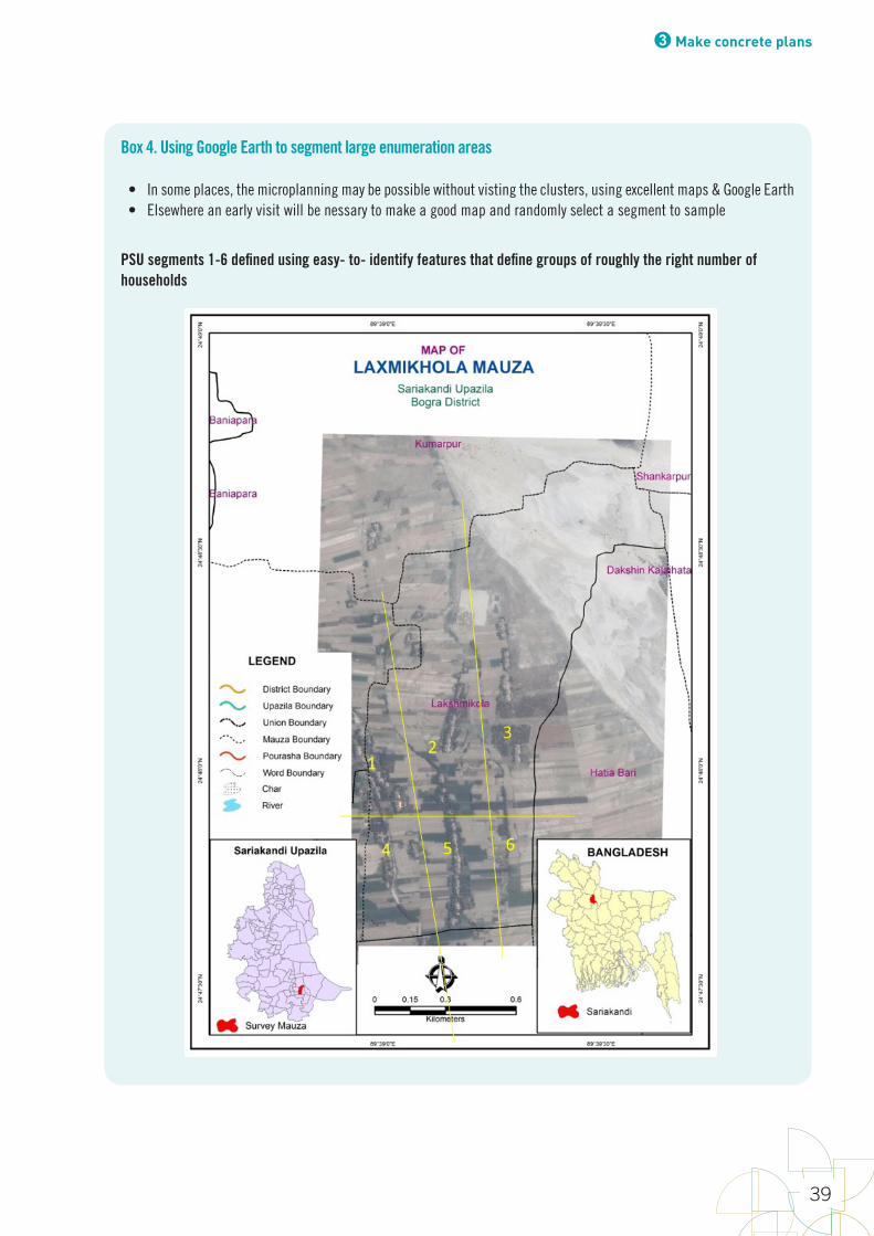
3 Make concrete plans
39
Box 4. Using Google Earth to segment large enumeration areas
• In some places, the microplanning may be possible without visting the clusters, using excellent maps & Google Earth• Elsewhere an early visit will be nessary to make a good map and randomly select a segment to sample
PSU segments 1-6 defined using easy- to- identify features that define groups of roughly the right number of households
World Health Organization vaccination coverage cluster surveys: reference manual
40
5. Choose a random number (x1) between 1 and the sampling interval. Compare this number with the cumulative population sizes to identify the first selected PSU. A PSU is selected if the random number chosen is greater than the cumulative size measure of the preceding PSU, but less than or equal to its own cumulative size of measure. The first PSU in the list is chosen if the random number is smaller than the size measure of the first row.
6. Calculate the next number (x2) = x1 + sampling interval, to determine the next selected PSU.
7. Continue x3 = x2 + sampling interval, and so forth until the desired number of PSUs is selected.
The worked example in Annex D shows you how to combine systematic PPES sampling with geographic arrangement of the sampling frame to achieve implicit stratification by urban/rural residence.
For special population such as refugees or internally displaced persons (IDPs), vaccination coverage survey sampling recommendations will vary depending on the phase of the emergency. In stabilized situations, it will be important to include refugees and IDP populations into the national coverage surveys with consideration given to ensure the sampling frame includes camps and other areas hosting refugees and IDPs to have a representative sample including these populations. In some contexts where refugees or IDPs represent a large proportion of the population, particularly where there is reason to suspect that coverage may be different among this group, oversampling may be considered to provide estimates for both the displaced persons and the host population. If these populations have recently been displaced and there is dynamic population movement, insecurity issues, and a different population size than is typically used for standard EPI surveys, other survey, or even rapid assessment, guidance may be used. It is often necessary to use data other than the national sampling frame in these settings. In addition, maps and up-to-date lists of residents may not be available during emergency situations. Therefore, different approaches to surveying these populations must be accounted for during the planning and execution of surveys. For guidance in planning a vaccination coverage survey in immediate emergencies, please refer to the UNHCR vaccination survey guidelines reference manual2, and 2013 UNHCR Standardized Expanded Nutrition Survey (SENS) guidelines (http://sens.unhcr.org).3
3.6.6. List households in selected clustersDepending on the survey goals, target age group(s), length of the individual questionnaires, and local demographics, survey planners may choose a single-stage design or two-stage design. In a single-stage design, all eligible children in the selected clusters are enrolled to participate in the survey. A two-stage design has an initial phase of household listing and random household selection, followed by a repeat visit to interview parents of eligible children.
For evaluation of routine vaccination coverage using a relatively short questionnaire (for example, one that does not have many extra questions on knowledge, attitudes and practice, or indicators related to other health programmes), a single-stage approach in which all eligible children in the selected clusters are enrolled is often more efficient than a two-stage approach. For example, if the survey requires 10 children aged 12–23 months per cluster, and the local birth rate is 30/1000 population and average household size is 5 persons, on average the number of households needed to enrol 10 children would be
49
------------------------------------------------------------------
Box4.UsingGoogleEarthtosegmentlargeenumerationareas
3.6.6. List households in selected clusters Dependingonthesurveygoals,targetagegroup(s),lengthoftheindividualquestionnaires,andlocaldemographics,surveyplannersmaychooseasingle-stagedesignortwo-stagedesign.Inasingle-stagedesign,alleligiblechildrenintheselectedclustersareenrolledtoparticipateinthesurvey.Atwo-stagedesignhasaninitialphaseofhouseholdlistingandrandomhouseholdselection,followedbyarepeatvisittointerviewparentsofeligiblechildren.
Forevaluationofroutinevaccinationcoverageusingarelativelyshortquestionnaire(forexample,onethatdoesnothavemanyextraquestionsonknowledge,attitudesandpractice,orindicatorsrelatedtootherhealthprogrammes),asingle-stageapproachinwhichalleligiblechildrenintheselectedclustersareenrolledisoftenmoreefficientthanatwo-stageapproach.Forexample,ifthesurveyrequires10childrenaged12–23monthspercluster,andthelocalbirthrateis30/1000populationandaveragehouseholdsizeis5persons,onaveragethenumberofhouseholdsneededtoenrol10childrenwouldbe+'#+'''&'#-
=66.7.Ifanenumerationarea(EA)containsonaverage100households,theaveragenumber
ofchildrenexpectedtobefoundinthatEAwouldbe+''#-#&'+'''
=15children.Itislikelytobemore
efficienttoenrolalleligiblechildrenintheEA,byvisitingallhouseholdsandenrollingeligiblechildren
= 66.7. If an enumeration area (EA) contains on average 100 households, the average number of children expected to be found in that EA would be
49
------------------------------------------------------------------
Box4.UsingGoogleEarthtosegmentlargeenumerationareas
3.6.6. List households in selected clusters Dependingonthesurveygoals,targetagegroup(s),lengthoftheindividualquestionnaires,andlocaldemographics,surveyplannersmaychooseasingle-stagedesignortwo-stagedesign.Inasingle-stagedesign,alleligiblechildrenintheselectedclustersareenrolledtoparticipateinthesurvey.Atwo-stagedesignhasaninitialphaseofhouseholdlistingandrandomhouseholdselection,followedbyarepeatvisittointerviewparentsofeligiblechildren.
Forevaluationofroutinevaccinationcoverageusingarelativelyshortquestionnaire(forexample,onethatdoesnothavemanyextraquestionsonknowledge,attitudesandpractice,orindicatorsrelatedtootherhealthprogrammes),asingle-stageapproachinwhichalleligiblechildrenintheselectedclustersareenrolledisoftenmoreefficientthanatwo-stageapproach.Forexample,ifthesurveyrequires10childrenaged12–23monthspercluster,andthelocalbirthrateis30/1000populationandaveragehouseholdsizeis5persons,onaveragethenumberofhouseholdsneededtoenrol10childrenwouldbe+'#+'''&'#-
=66.7.Ifanenumerationarea(EA)containsonaverage100households,theaveragenumber
ofchildrenexpectedtobefoundinthatEAwouldbe+''#-#&'+'''
=15children.Itislikelytobemore
efficienttoenrolalleligiblechildrenintheEA,byvisitingallhouseholdsandenrollingeligiblechildren
= 15 children. It is likely to be more efficient to enrol all eligible children in the EA, by visiting all households and enrolling eligible children immediately, than to have a first step of listing households, selecting 67 households randomly, revisiting those 67 households, and enrolling eligible children at the revisit. On the other hand, if a long questionnaire is to be administered to eligible individuals (that is, one that takes an hour or more to complete), it may take less time overall to use a two-stage approach so you are not interviewing more individuals than necessary. In surveys such as post-MR campaign surveys, which enrol persons of a wide age range and an eligible person is found in every one or two households visited, a single-stage approach would result in a sample size much higher than needed, and a two-stage approach may be preferred.
2 UNHCR (2017) Vaccination Survey Guidelines Reference Manual (Draft)3 UNHCR (2013). Standardised Expanded Nutrition Survey (SENS) Guidelines for Refugee Populations- Pre-Module: Survey Steps and Sampling, Version 2
3 Make concrete plans
41
Whether a single-stage or two-stage design is used, a household listing step is essential (see Annex F). In each cluster, survey teams list each structure on a listing form, noting which are inhabited and which are not (for example, schools and offices). See Form HH in Annex H for an example. Interviews are conducted at each household to record the names of the heads of the households and the household composition on this form. In a single-stage design, this is done concurrently with enrolling eligible persons, and it facilitates quality control of the completeness of the fieldwork and provides the data needed for the weighted analysis. In a two-stage design, the listing enables the coordinator to select a random sample of households for field teams to visit at the second stage to collect vaccination data. In both designs, up to two revisits should be conducted, if needed, to obtain all the information for all eligible persons.
If no one is at home, it may be possible to ask neighbours whether any eligible respondents live in the household. Form HH lists a field to indicate whether the information about the household comes from a resident or a neighbour.
Regardless of whether the survey uses a single-stage or two-stage design, the outcome of all visits to households in the survey sample must be carefully documented. Children in households with an available and willing respondent may be more likely to have been vaccinated than those in households with unavailable or uncooperative respondents, so careful accounting for missing data is needed to reduce bias in coverage estimates. Form HM in Annex H lists a space for a disposition code (interview outcome code) for three visits to every eligible respondent in the household.
3.6.7. Collect data on vaccination from eligible persons in each household selected for the sampleIn single-stage designs, all households in the cluster are screened and all eligible persons are included in the sample. It is essential to visit all dwellings, list all households, and enrol all eligible individuals in the cluster, no matter what the estimate target number of respondents per cluster originally was in sample size calculations. In two-stage designs, a random sample or systematic random sample of households within the cluster is pre-selected and the list given to field teams. All households on this list are visited, and if an eligible person lives there or has spent the previous night there, a vaccination questionnaire is completed.
Up to two revisits should be done as necessary to complete vaccination questionnaires as fully and accurately as possible. If a respondent is not present at the first visit, do up to two more visits to meet them. If a respondent (for example, the caretaker of a 12–23 month-old child) is present at the first visit but the home-based record is not available, then complete as much of the questionnaire as possible at the first visit but do up to two more visits to review the home-based record and complete the relevant section of the questionnaire.
To have enough time for high-quality household listing, enrolment of eligible persons and collection of complete and high-quality data, it is likely that more than one day will be needed in each cluster, whether a single-stage or two-stage design is used. Exceptions may be for post-SIA coverage evaluations for national-level coverage estimates of an SIA that targeted a wide age range (such as MR campaign of children aged 9 months to 14 years, or meningitis A campaigns of persons up to age 30 years). As few as five households may be needed in each cluster, and the questionnaires are short, so it may be possible to do the household listing and mapping in the morning and revisit the few selected households in the afternoon (for an example, see Meyer et al. 2015). Revisits of households where a respondent was absent at the first visit are still required, however, which might still require a second day of fieldwork in the cluster.
3.7. Obtain access to health registers for vaccination recordsThe value of adding visits to health facilities in order to seek more documented evidence of vaccination (for example, for children whose home-based records (HBRs) were not available) will depend on many factors. One of the most important ones is the likelihood of finding vaccination records in the facility that are complete and organized in a manner that allows tracking the

World Health Organization vaccination coverage cluster surveys: reference manual
42
records needed for specific children. In setting where HBRs are less available, oftentimes health facility vaccination records are also less likely to be of quality or properly archived. These surveys are precisely the ones that would benefit most from having a higher proportion of children with documented evidence of vaccination. Visits to health facilities while planning the survey may help you better understand the practices related to record keeping and the feasibility of identifying vaccination records for selected children. To add value to visiting health facilities, and offset costs, some surveys have added interviews to health workers about immunization or data quality assessment activities, such as reviews of data in tally sheets and registries, and comparisons with the data reported in the monthly report form.
It will be necessary to search for evidence of vaccination status in health facility records for children in the cluster whose caretaker says that they received some routine vaccinations locally, and if:
• the caretaker does not show interviewers the vaccination card, or
• the card indicates some doses with a tick mark, but no date, or
• the caretaker says that the child received some routine doses that are not recorded on the card.
If you decide to access to health facility records to check the vaccination status of some of the children, it is wise to budget the additional time and resources necessary to do this. Plan to visit all health facilities that vaccinate children in the survey clusters to establish collaboration, gather early documentation (copies of the records), and assess the health register quality (legibility of the records).
Before fieldwork begins, obtain lists of the names of the vaccination providers (including private ones), health facilities, and outreach posts with their geographical catchment areas. It is best to obtain these lists from the district director of health or the EPI manager, whom the survey coordinator should visit anyway as a courtesy before teams go into the field. You should also ask local guides for the names and locations of vaccination places the local population uses. If it is common in your country for children to receive vaccinations from private providers, the steering committee may decide that data collectors should visit the private providers’ offices to obtain records for children whose home-based records are not available. When surveying IDPs during or after a crisis, try to locate the health register data at refugee camp health facilities.
It may be more cost-effective to finish the list of children whose records need to be searched and have a different team collect the data in the health facilities. Taking pictures of the registries may also be useful to verify the data collected.
Be aware that even the original health records could be hard to decipher and may require clarification from the original writer.
3.8. Select and hire staffOver time there has been a growing trend to subcontract vaccination coverage surveys to private or research institutions. If the survey is subcontracted, all requirements of the survey, including provisions for data ownership, should be spelled out in detail in the request for proposal (RFP), and the submissions scrutinized for their exact adequacy adherence to the terms of reference.
One key staff person is the survey coordinator. The coordinator has authority over everyone involved in the survey, and works directly with whomever requested the survey.
The coordinator is responsible for:
• overseeing the implementation of the vaccination coverage survey
• ensuring the cooperation of other relevant government agencies

3 Make concrete plans
43
• making budget estimates for the survey before potential funding sources are identified for the survey
• ensuring proper selection of field teams
• overseeing the fieldwork
• reporting survey results
• overseeing training and pilot testing
• overseeing data entry and data management
• overseeing data analysis and report writing.
Whether directly hired by the survey coordinator or indirectly by a contractor, all types of workers who will be involved with the data collection and analysis must be identified and selected. The coordinator or the contractor must select people capable of working as members of a team and qualified to undertake their respective roles, as defined by the job description. The coordinator or the contractor should establish the required profile of each type of staff for the tasks they have to perform.
The data collection and analysis process have several consecutive steps, each involving its own team of skilled workers:
• data collection, with a team of field interviewers and supervisors (in two-stage cluster surveys, the data collection team may be subdivided into a household mapping/listing team and an interviewing team)
• data entry, with a team of computer operators, data cleaners, and supervisors
• data analysis, with data analysts producing the tables already defined by the steering group and agreed upon with senior officials and partners requesting the survey.
Each step of the process requires a thorough data-checking process that includes all of the following:
• in the field by the interviewers (checking each other’s forms for completeness and accuracy) and supervisors (checking forms, observing interviews, conducting repeat interviews)
• by the data entry staff at the time of the dataset is created (creating the dataset by using a double entry process and by inserting limits for each field)
• by the data analysts (checking the consistency and range of the data).
3.8.1. Field staff
Regional coordinators
Regional coordinators are responsible for the fieldwork in one or more strata of the survey. They check the quality of maps and microplans. Similarly, they assist supervisors and interviewers to be able to find the appropriate clusters, communicate with each supervisor daily, and make others aware of progress and changes in plans. Regional coordinators also work to ensure consistent responses to unforeseen developments. Supervisors report daily progress to the regional coordinators, and in turn the regional coordinators report the progress up to the survey coordinator.
Regional coordinators also conduct quality checks by revisiting a portion of households already surveyed to verify that the household listing and interviews were conducted properly, that all eligible respondents in those households completed questionnaires, and that vaccination dates (and possibly other responses) were recorded correctly in homes where cards are available.

World Health Organization vaccination coverage cluster surveys: reference manual
44
Interviewers should know ahead of time that a proportion of households will be revisited by regional coordinators, or by other independent monitors, but should not know which ones.
Field supervisors
Field supervisors have several roles. They must make sure that the fieldwork of their teams is performed according to standards. Although the supervisor cannot be with every team every moment, this person is expected to be in the field, observing the teams as much as possible. Field supervisors are also the first-line reference for clarification in case the interviewer has doubts. They must also flag inconsistencies in the questionnaires, and update the survey coordinator on the progress of their teams.
Too often, supervisors are selected at the end of the training from among the brightest trainees. This may be inadequate for several reasons. Supervisors do not only need technical skills, but also the capacity to lead a fieldwork team, and to monitor and constructively correct poor practices of field interviewers. Also, specific training on these skills may have to be organized at the same time that interviewers are trained to interview, or right before, so that supervisors can also help facilitate the training of interviewers.
Field supervisors are responsible for:
• ensuring the welfare and safety of the team
• ensuring each member of their teams is fluent with the questionnaires and techniques of the interview
• ensuring each member of the team has the necessary materials for their his or her daily activities
• overseeing the activity in the field
» confirming that a verbal history of vaccination is obtained using the standardized approach, agreed upon during training, so that the language does not bias the responses
» confirming that adequate time is allowed for the respondent to look for all available home-based records
» checking that field staff do not make transcription errors when copying down dates from the cards or health facility records
» visiting every home in a sub-sample of clusters to confirm that each was visited and revisited if necessary.
• reviewing all forms before leaving the cluster (perhaps at the end of each day) for legibility, completeness, and accuracy, and the use of photos of cards when possible
• ensuring that completed data collection forms are given to those responsible for data processing in a timely fashion
• checking the quality of photos.
Interviewers
Interviewers work under the supervision and guidance of the field supervisor, and are responsible for collecting the data according to the instructions given in the data collection instructions to the forms. They are accountable for the data they collect and the way they collect it.
Below are some things to consider when selecting interviewers.
• Interviewers should have a sufficient level of education (defined nationally), a pleasant personality tuned to local social customs, enough physical stamina to walk long distances under rain and sun under through sometimes difficult terrain at times, and a fluency in the language(s) spoken by the interviewees.
• Depending on the local customs, it may be necessary to have the correct mix of male and female members of the field teams. In some cultures interviews can only be conducted between people of the same sex, and in some cultures female interviewers must be accompanied by a male staff person.
3 Make concrete plans
45
• It may be an advantage to hire field interviewers who have worked on other surveys. Although they have demonstrated they can perform under field conditions, their previous experience may give them a false sense of confidence and weaken their capacity to pay attention to the specific requirements of the new survey. It can be beneficial to include an interviewer with census experience in each survey team, in case there is a need to do sketch maps.
• Interviewers must be able to write carefully and clearly, especially numbers. If using CAPI, interviewers must be able to correctly operate the data collection device to be used for the survey.
• The survey coordinator or the contractor should avoid using health or EPI staff as interviewers when possible.
» People associated with the vaccination services (local EPI staff) may unwittingly influence the way respondents reply to some questions, particularly those relating to reasons for not being vaccinated. However, people unfamiliar with the vaccination services may not naturally probe for important information on vaccination age, dates, and reasons for failure, and may also confuse dates that they see on a card (for example, the proposed return date with the actual date of vaccination). This is why it is important to train interviewers thoroughly on vaccination practices and on the rationale of the survey questions. In case no local candidates are found, the coordinator may consider hiring a health or vaccination staff member from another area, if the candidate can speak the local language.
Drivers and local guides
Drivers are responsible for the proper timing of the daily activities, and for the reliability and safety of the teams’ transportation to and from sites. This is a very important role, so drivers and guides must be made to feel part of the team and feel accountable for the timely conduct of the survey.
The selection of a local guide is not usually the responsibility of the coordinator. Usually the coordinator makes arrangements with authorities in the areas to be covered by the survey cluster or health facilities, to assign guides to the field teams.
The role of local guides is to:
• help field teams familiarize themselves with the clusters they are to survey
• introduce them to the cluster’s administrative and social authorities
• advise survey staff on when it is best to visit households
• introduce field teams at houses if requested by the interviewers.
Local guides should not be involved in deciding which dwellings to visit, or in interviewing and collecting data.
Observers
The coordinator may decide to include international or national participants, observers or monitors to enhance the confidence and objectivity in the results of the survey.
3.8.2. Data management and analysisInformation communication technology specialist
Where data is collected using CAPI on mobile devices, the information communication technology (ICT) specialist is a full-time position based at the central office. This person is responsible for receiving the daily data collection on the server, checking the coherence of the data, and returning any problematic data to the field that night to be checked and corrected the next day.
World Health Organization vaccination coverage cluster surveys: reference manual
46
Data manager
The data manager is a full-time position worker responsible for designing the database structure and the data entry interface. This person verifies that all data (GPS coordinates, questionnaires from households and from health centre registers, photos of cards, etc.) have been sent daily, monitors the data checking process, and verifies that the monitoring tools have been filled out daily by the supervisors and given to the survey coordinator. Monitoring tools include the numbers of household visited, percentage of questionaires completed, percentage of persons whose vaccine records were extracted from the health centre registers, etc.
The data manager also merges files from the data entry operators, and ensures that the paper forms are correctly archived and stored, copies of the data file are free of viruses, and the data file has been copied for backup purposes. Finally, the data manager is responsible for training and supervising the data entry operators.
Data entry operators
Depending on the number of computers available for data entry, more than one shift of data entry operators may be employed to complete data entry. When using double shifts, avoid inconsistencies by training all data entry operators and their managers uniformly, so all managers give the same answers to the same procedural questions. Data entry operators should be identified and trained shortly before data entry begins.
Statistician
The statistician contributes at several stages of the project, first working closely with the steering group and later working closely with the data manager. In early conversations about the survey goals, the statistician calculates sample sizes to meet the objectives identified by the steering group. Later, the statistician reviews the proposed questionnaires and works with the data manager to define the database design, design a codebook, and specify appropriate checks on valid ranges of values for survey responses.
The statistician also helps to evaluate candidate sampling frames for clusters, may conduct or help with cluster selection, and contributes to the microplanning protocol to be sure that microplanners save information that will be needed to calculate survey weights. Likewise, he or she works with the steering group to draft table shells and identify graphs needed for the survey report. When a sample dataset is available, the statistician also writes well-documented statistical code to check the dataset, identify unexpected data values, calculate derived variables, populate table shells and generate figures.
After the data is analysed, the statistician helps draft the methods, results, and strengths and limitations sections of the report, and works with other authors to be sure that results are interpreted clearly and correctly. The statistician populates individual variable summary tables in the final codebook and, when appropriate, makes both the dataset and analysis code available for checking by independent parties.
When CAPI is used to collect data in the field and upload it to a server, the statistician works with the data manager to create tools to summarize the data collected thus far, and to identify problems based on whether data are missing or have strange values, or whether the latitude and longitude of each team’s data are in the expected location of the clusters.
3.9. Train staffA good survey requires dedicated and motivated interviewers who understand the importance of the survey and their role in it, and have mastered the use of good tools. The acquisition of the needed skills is the result of the quality of the individual candidates and their training.

3 Make concrete plans
47
Final interviewer selection should take place at the end of the training session. Candidates with poor handwriting or those who still have an incomplete understanding of the forms should not be selected. Train more people than needed so you can select the best, and also have additional trained workers available in reserve in case several selected workers default for sickness or other reason.
3.9.1. Training time and number of traineesAnnex G provides helpful training tips. Training should be given considerable attention and time. Do not rush the training, and confirm that the information presented is clearly understood by all trainees. In addition to training on the survey process and tools, supervisors need training in supervisory skills and in how to do field checks for data quality.
It may require multiple checks to ensure that the staff has acquired the necessary skills. Not doing so will jeopardize the quality of the results. This is why each instructor should be limited to 20 trainees, so the instructor can devote sufficient time and attention to each trainee. Having even fewer trainees per instructor may be even better.
A minimum of five days is generally required for the initial training, the field pilot test, the analysis of the pilot test data (to identify individual mistakes or the flaws in the instruments), direct feedback and potentially revising the tools. Enough time should be allocated to ensure that field staff understand how to identify the boundaries of the selected clusters or segments, how to do the household listing, and how to complete the individual questionnaires correctly. If there are several variations in vaccination cards or EPI register books in circulation, interviewers should learn to recognize and extract data from each type.
3.9.2. Training topics and methodsProvide training on how to handle common problems with household-level data collection. Useful areas to address include:
• what to do with several households in a common dwelling
• how to define the date of birth if it is not clearly written in the card
• how to deal with incomplete or illegible dates or errors in the chronology of dates of birth and vaccinations
• how to document a vaccination history from the caretaker, and what to do if there are incomplete forms or absent cards, or if the caretakers are not present.
For training on using health centre records, focus on the most common problems:
• inability to access the records (staff out of station, records in the field, records already archived elsewhere, etc.)
• inability to locate the child from the records due to misspelling of the child’s or parent’s name
• inability to locate the child in the records due to registrations organized by day instead of alphabetically or by card serial sequence.
Training methods should be as practical as possible. Include instruction on a standard way to write numbers clearly (with handwriting exercises if paper forms are used), and on how to review incorrectly filled forms. Include role plays on how to do introductions, ascertain dates and assess likely vaccinations from caretakers. Close observations during training and the pilot field test will allow the trainer to give immediate feedback and corrective action. Such training is necessary even when field staff will use digital data entry.
Consider doing a video recording of the pilot field practices of the trainees (budget for this in advance). The day after the field pilot test, the parts of the videos documenting shortcomings or errors should be shown and discussed. A good technique is to let the trainees discuss what is wrong or could be improved in that section of the video


4Conduct field work
4.1. Collect data from households
4.1.1 Visit all households selected for interviewsHigh quality data collection (including the revisit of households initially found vacant) will probably require field staff to spend more than one day in each cluster. Sometimes evening or early morning visits will be required. The interviewers may spend the night in the cluster if it is logistically possible and safe. The logistical arrangements should allow the interviewers to start early enough to find children and their caretakers at home.
Sometimes evening (or early next morning) visits will be required. Some interviews may need to take place in the evening after caretakers have returned home. In these cases, local guides may be even more important to obtain access to houses. Evening visits may have to be done by male interviewers if security is a concern, or if cultural considerations require it.
Young children do not need to be physically present at the time of the interview, but a caretaker or knowledgeable guardian, ideally someone who can supply the child’s vaccination card, must be present to proceed with the survey. Nevertheless, when vaccination has taken place in schools, and with older children, it may be beneficial to have the child present, as the caretaker may not know about the said vaccination. If no knowledgeable caretaker or card is available during the first visit, a second and third visit in the evening or on the next day should take place before the interviewer leaves the cluster. Record the interview outcome for each visit using a disposition code on Form HM.
The total counts of eligible children in each cluster will be used to calculate survey weights. Putting zero or indicating a missing value for households would lead to an underestimation of the total. So, if no one is at home during the initial visit, some survey protocols will allow interviewers to ask neighbours how many survey-eligible children live in a household where no one is at home at the time of the initial visit, and to record this information on the household listing form (Form HH in Annex H).
4.1.2. Conduct the interviewAfter introducing themselves and explaining the purpose of the survey, the interviewers should establish whether anyone in the home is eligible (spent the previous night in that household and is of the appropriate age group), and if so, obtain informed consent to administer the questionnaire. In most cases, ethical review boards will allow a protocol to use verbal informed consent only if the survey does not include taking biological samples. If the coverage survey is combined with a serosurvey, then the protocol may involve having an adult sign a consent form.
To ascertain the eligibility of a person it is necessary to identify his/her age and therefore the date of birth. This can be done from the vaccination card, or a birth certificate, if available. If a card is not available, the date of birth should be reconstructed from a calendar of local events (prepared during training): religious festivals, political events like elections, climatic events (monsoons, cold weather), etc. It might be time consuming but is essential.
After obtaining consent to proceed, begin the interview, following the logical flow of the questionnaire. The availability of a vaccination card should be immediately assessed using the specific questions in the questionnaire (Have you ever been given a card? Do you still have it? Can you bring it?). It is vital to give the caretaker time to find the card, and to offer to return at a later time if necessary (for example, if the card is in a locked cupboard and the father has the key and will return later that day).
If a card is available, the interviewer should check the date of birth and available dates of vaccinations for legibility and consistency. The card should be interpreted according to the format used in the area. For example, sometimes a date written in pencil means the date the child should return for the next dose. The protocol should be clear about any local or national practices that could be confusing to survey staff.
World Health Organization vaccination coverage cluster surveys: reference manual
50
If there are no written dates for a vaccination the child is eligible for, the caretaker should be asked for a history of that vaccination, using the national EPI body site for each injection, such as right arm or left leg, as a reference. The interviewer should also ask about the name of the place (health facility, outreach site, etc.) where each vaccination was received to facilitate obtaining the health record from the health register. 4.1.3. Refer unvaccinated children to the health centreIf the interviewer learns that a child in the household is overdue for a vaccine, he or she should recommend that the caretaker take the child to the health centre to receive the vaccine. Before the survey begins, you may ask the ministry of health to create a referral letter for this purpose, and give a copy to the child’s caretaker. Give the health centre a copy in advance so they are aware that the survey team may refer a small number of unvaccinated children over the age of 12 months. Also give a copy of the letter to the caretaker of any child that should be referred to the health centre for a vaccine.
4.1.4. Check the completed questionnaireEvery completed questionnaire should be checked by the interviewer first, and later by the supervisor. Every question of the form should be filled in clearly and legibly. If one interview team member writes the dates, then before leaving the home, the other team member should check the form to verify the correctness and legibility of the dates. The dates on the questionnaire must match what was recorded on the vaccination card, even if the vaccination card has invalid dates. The data manager or field coordinator, not the interviews, must decide how to handle such dates. If the protocol includes taking a photo of the vaccination card, the photo should be checked for clarity. Additional photos should be taken, if necessary, to eliminate a bright glare, dark shadow, or blurriness.
The supervisor must verify every questionnaire for completeness, consistency, and legibility, and also evaluate photos for clarity and completeness. If there are errors in completing the questionnaire, the interviewer must correct them before leaving the cluster.
4.2. Check health registers from the health centre See section 3.7 for guidance on when it is appropriate to check health registers. If the team plans to check health registers, the first task is to find the child in the health register:
• Narrow the time period to match the month and year of birth with the month and year of the record pages;
• In case of a health record issued serially with the vaccination card, try to match them;
• Try to match the name of the village, hamlet, or administrative unit from the questionnaire with that on the register; and
• Try to match the name of the child as well as the names of the father and mother. Often people have two names (their official administrative name and their usual name), which makes matching difficult. In some cultures, very young infants do not receive a name until several weeks after birth.
After the child’s record is found in the health register, the team should copy the data from the vaccination record on a separate health centre form (RIHC questions in Annex H).
Some surveys may include up to three types of vaccination information for each child:
• vaccination history according to the card
• vaccination history according to the caretaker’s recall
• vaccination history according to the health registers.
4 Conduct field work
51
Sometimes these sources will have discrepancies. The data collection field teams do not need to make any decisions in case of discrepancies, but simply to record verbatim what has been found. At a later stage, data analysts will describe and address the discrepancies, carefully documenting each decision they make about editing data in the database and why.
4.3. Monitor the quality of field data collectionA quality survey depends on the work done in the field. There are several potential sources for error in the data, and the interviewers, supervisors, and field coordinators have the primary responsibility for identifying and correcting errors in the initial collection and recording of the data.
4.3.1. Re-check households with no eligible children
If the household listing form says that there is no eligible child in the household, check the household again to be sure.
4.3.2. Check completed questionnaires Responses from the child’s caretaker, the home-based record, or the health register may be missing, illegible, or in error. The interviewer may have misunderstood the child’s caretaker or misread the home-based record or health register. The interviewer may also have forgotten to enter the information or may have entered it incorrectly.
Each form, and ideally each page on the form, should contain the following information, and supervisors in the field should check each questionnaire for these items: • Form number: Each questionnaire should be assigned a unique form number to facilitate checking the data entered with
a paper form.
• Cluster number: A cluster number should be entered for each form, because the data cannot be properly analysed if there is no cluster number. Ideally, clusters should be numbered from 1 to the total number of clusters. For example, if data are being collected for 30 clusters, clusters should be numbered from 1 through 30. Although census bureaus usually assign a much longer and more complicated identification (ID) to each EA to indicate province and district location as well as a rural/urban distinction, these long sequences of ID characters are subject to transcription errors and should be avoided in field paperwork. The survey data coordinator can maintain a list that matches the simple survey cluster number from each stratum (for example, 1–30) to the complete and specific EA number provided by the census bureau.
• Household number: The household number is a combination of structure ID and household serial number, as recorded on Form HH (see Annex H). The household number for each household in which an eligible child has been interviewed should be recorded to facilitate data checking. Since several interviewers are likely to be working in the same cluster, each interviewer should be assigned a set of structure numbers in advance (for example, 100–199, 300–399).
• Household resident number: A resident number must likewise be entered for each form so that the data can be properly analysed. Household resident numbers are assigned within households and range from 1 to the total number of residents in the household. Forms RI, TT and SIA in Annex H include a place to record the resident number for each child and caretaker from Form HM. It can be helpful to record the child’s first name as well. (Note: During data cleaning and management, each child will be assigned a unique ID in for the survey, consisting of a combination of stratum ID, cluster ID, household ID, and household resident number. It is not necessary to construct this unique number in the field.)
• Child’s date of birth: The child’s date of birth should be entered on the questionnaire and checked to ensure the date of birth is between the eligible dates of birth for the age cohort.
• Date of interview: The date the interview was conducted should be recorded and checked.
World Health Organization vaccination coverage cluster surveys: reference manual
52
• Dates of vaccinations: Vaccination dates should be between the date of birth and the date of the interview. The answers to questions on dates of vaccination should be consistent with the response to the answers about the presence of a home-based record. If there is no home-based record, or the card had only a tick mark, there should be no dates of vaccination, and instead, there should be answers on the caretaker’s verbal history of vaccination. For such children, vaccination dates will be sought in the health facility and recorded on a health facility form.
• Home-based record (vaccination card): If the completed questionnaire indicates that there is no home-based record for an eligible child, check to make sure this is actually true.
• Other fields should have an entry within the range of acceptable entries.
• Finally, a field for comments about the interview is often useful, even when data is collected using mobile devices.
Each data collection form should have an entry for each field (unless some questions cause others to be skipped) and the responses should be legible. In general, in survey forms, text in lowercase represents what is to be read as part of the interview and text in uppercase represents text that is not to be read, such as instructions to interviewers. Each form should have a correct cluster and household resident number entered. Only those who meet the eligibility criteria should be included in the sample.
There are several levels of quality monitoring expected in the field:
1. Each interviewer is expected to submit only completed, legible, and accurate questionnaires. When there are teams of two interviewers, it is useful to have each worker check the other’s questionnaires after completion.
2. Every day, the supervisor must check every questionnaire for completeness, legibility, and accuracy. The supervisor checks that the household list indicates that questionnaires have been completed for all eligible children, and if not, there are reasons recorded for missing questionnaires (for example, caretaker not available after two visits or refused to participate). All forms must be checked and corrected before leaving the cluster area. The supervisor’s signature on the questionnaire confirms that this was done.
3. The survey coordinator or contractor is expected to organize a revisit of 10% (as an ideal) of all eligible children a day or two after they have been visited, to be sure that maps were followed correctly, cluster or segment boundaries were correctly identified, and that fieldworkers did not skip (either intentionally or by mistake) interviews for eligible children. Because the coordinator’s priority is to support the ongoing survey activities, it is not practical for him/her to do all of these revisits alone. Instead, the survey team should budget for a dedicated supervisor or two to be assigned to that task. Contractors may resist this provision, but it is a recommended practice. A 10% sample of clusters should also be revisited for repeat household listing, to check that the household lists have been done correctly and tally eligible respondents in each home. The children to be revisited can be selected randomly or not, as the coordinator may have doubts on specific questionnaires. When revisiting the households, the supervisor should ask the caretaker to repeat the interview for the sake of quality control, and compare the resulting questionnaire’s results with those of the interviewers.
Supervisors should give feedback immediately to interviewers about any discrepancies, correct the discrepancies, and discuss steps to improve the next day’s work. Any discrepancy or missing data should be resolved by discussions with the interviewers, a review of photographs of the vaccination card (if available), or revisits to households if necessary.
4.4. Check questionnaire forms and transmitThe data collection team should count all questionnaire forms and verify them against the household lists. Once the questionnaires and health register forms have been checked by the supervisor, the supervisor should send them to the survey coordinator through safe channels as soon as possible, to be entered into a database. When data is collected digitally through smartphones or other portable devices, it may be easier and faster to transmit the data to the survey coordinator provided that there is good connectivity, than when paper forms are used.
4 Conduct field work
53
4.5. Clusters that become suddenly inaccessibleAs the survey progresses, situations can change and some clusters may become suddenly unsafe due to nearby hostility, wildfires or flooding. If safe access is expected to be restored during the period of field data collection, make every reasonable effort to retain the originally selected cluster in the sample. (For example, a flooded river is expected to recede.) This may require postponing data collection in that area and coming back toward the end of the survey. This is the most desirable outcome from the perspective of data integrity and representativeness. If the problem persists and there is no reasonable expectation of being able to collect data in that cluster as planned, then the survey steering group will need to determine whether to select a replacement cluster, and how the data analysis should account for the missing data from the originally selected cluster.
If the factor that made the cluster inaccessible to the survey team might also periodically make the same cluster inaccessible for vaccine delivery, that cluster might have especially low vaccination coverage and leaving it out of the survey might bias results upward. Some sensitivity analysis might be required to understand what the effect of finding low coverage in that cluster would have been. On the other hand, if the inaccessibility during the survey was clearly not related to anything that might have affected vaccination coverage (for example, these were the first wildfires in the region in over five years), the steering group may decide simply to substitute another randomly selected cluster for the inaccessible cluster and skip the sensitivity analysis.
The safety of the survey personnel is of primary importance, of course, and decisions about survey operations should ensure as safe a working environment as possible. If some originally selected clusters are omitted or replaced during the fieldwork, then the survey report should document clearly what was done and indicate the reasons for omission, speculate about whether these causes might also affect vaccination coverage there, and document any sensitivity analyses.
World Health Organization vaccination coverage cluster surveys: reference manual
54

5Data entry, cleaning
and management
This chapter describes steps necessary to prepare the data for analysis. Some surveys use paper to record interview responses and others use CAPI to record, store and transmit data.
5.1. Database design Design and test a database in advance of the survey completion. Develop the database structure, create data entry routines and entry range checks and complete consistency checks. The database structure should be complete and accurate, and tested with pilot data so that the development of the statistical analysis programs can begin as soon as possible. The data manager is responsible for designing the database structure and the data entry interface.
Construct a complete list of survey variables, known as a data dictionary or codebook, at the same time the database structure is established. Each variable will have a type (string or number), a label, and a set of valid values. Categorical variables should have clear, concise labels for each category. Responses like “Do not know” or “Refused to answer” should have well-defined values in the codebook and in the data entry software. After data has been collected, the codebook can be updated to include a brief summary of each variable in the dataset. Section 5.5 describes the components of a useful codebook.
In most cases, each child will be represented with one data record. If the survey collected data on more than one cohort of subjects (for example, a cohort of children 12–23 months of age surveyed for routine vaccination, and a second cohort of women who have given birth in the last year surveyed for tetanus toxoid coverage), it is advisable to have a separate database for each cohort.
When responses are recorded on paper and entered later into a computer, the data entry form should look as much like the paper data collection form as possible.
Data entry operators may make errors such as typing a response inaccurately, not entering records (or entire forms) completely, or entering forms multiple times. The database should be designed to catch or prevent as many of these errors as possible, using appropriate filters and error checking. The software should accept only valid values for categorical variables and should provide a warning when data appear illogical (for example, the date of the second dose of the oral polio vaccine (OPV2) is earlier than that for OPV1).
If the data will be analysed using the WHO Vaccination Coverage Quality Indicators (VCQI) tool, it will be more efficient to use variable names and coding conventions listed in the VCQI Forms and Variable List (FVL) document (WHO, 2017, available on the web http://www.who.int/immunization/monitoring_surveillance/routine/coverage/en/index2.html ).
5.2. Data entryDepending on the number of computers available for data entry, more than one shift of data entry operators may be employed to complete data entry. When using double shifts, care should be taken to avoid inconsistencies by training all data entry operators and supervisors uniformly, so all supervisors give the same answers to the same procedural questions. Data entry should take place in a separate room from other survey activities, where the staff is not disturbed and the questionnaires are secure. Each data entry operator should be assigned a unique staff ID number that they enter with every record so feedback can be given to the right people if data quality audits reveal too many data entry errors. To reduce data entry errors, have each data form entered independently by a second data entry operator, and then compare the two entries using computer software (see section 5.3).
Once all the data is entered, the data manager must merge files from the different data entry operators, and ensure that the paper forms are correctly archived and securely stored in a fireproof and dry location that also ensures confidentiality. Only a
World Health Organization vaccination coverage cluster surveys: reference manual
56
limited number of survey staff members should have access to forms or photos that contain personally identifying information, and they should be well trained on how to do their work without revealing the identity of participants to other people who do not need to know that information. The data manager should also check that copies of the data files are free of viruses, and should backup data files regularly. In some instances, it may be important to document and manage different versions of the master data file to ensure the correct version is being used, and many available software packages have methods to do this automatically.
5.3. Clean the datasetThe data manager should work with the statistician to clean the dataset and create a series of checks for every variable in the dataset. The data cleaning step, when performed over all variables and all records, is time-consuming, but it is important to devote adequate resources for it. It is not sufficient to spot-check a subset of variables or a subset of records. Computer software should compare every variable and every record in the dataset, and all inconsistencies should be resolved before the data are summarized and analysed.
The data manager must have a plan for what to do when there are errors, and must follow the plan consistently. If the data management team changes any values in the dataset, the change should be documented in a data cleaning log. The change should be made using software, not by changing the value in the original dataset. This makes the changes reproducible and makes it possible to reverse the changes if they are later overruled. The software should include either comments or variables that capture the reasoning behind the decision to change a variable’s value. The sections below provide suggestions for handling different types of errors.
5.3.1. Duplicate, missing, or conflicting dataThe data manager should check for duplicate entries or forms that were not entered. When entries for one or more fields differ between the two versions entered, the data manager should refer to the original data collection forms (and, where relevant, photographs of home-based records or health facility registers) to determine which entries are correct.
5.3.2. Implausible or illogical responses The values should be checked to be sure they are plausible, and any logical relation should be checked to be sure the relation holds. Some examples: every vaccination date for a particular child should fall between that child’s birth date and the date of the interview, every record from a particular cluster should have been collected on the dates that the team visited that cluster, and every record from a single geographic stratum should have latitude and longitude values that fall within the boundaries of that stratum. The data manager should document any checks done for plausible values or logical relations.
The data manager should correct any implausible values found. Consult the original paper form, photograph of the vaccination card, or health facility record in case the problem occurred during data entry. If the unlikely or invalid value occurs on the original document as well, then the problem should be noted. When it is obvious what the correct value should be (for example, when dates fall in early January, it is common for people to continue to write the previous year), the value can be re-coded, but the decision to re-code responses from the value given to another valid value should be considered soberly. This serious action must be justified, documented clearly, applied consistently, and noted in the final report. If there is any ambiguity at all about the correct value, the safest course of action is often to set improbable values to “missing” and document that decision. If the incorrect value is a vaccination date, set the date to “missing” and include a tick mark variable to indicate that the child received the dose, but we do not know the correct date.
5 Data entry, cleaning and management
57

5.3.3. Skip patternsSome complicated forms use skip patterns, where one response on an earlier question causes the interviewer to skip later questions. For instance, in the verbal history portion of the questionnaire, if a caretaker says that a child has never received any vaccinations at all, the interviewer would skip the specific questions about BCG, OPV, etc. When data is collected using CAPI, the skip logic is usually programmed and tested, and is performed automatically. But when data are collected using paper forms, it is common for interviewers to inadvertently ask questions they should have skipped, or fail to ask questions they should have asked.
Data checking should include a step to evaluate whether skip patterns were correctly observed. If a question should have been skipped but data was recorded and entered, change the response to “missing” and document the change.
5.4. Merge datasets and construct derived variablesThis manual gives broad guidance, which may be made more specific by consulting with the statistician who will analyse the survey data.
5.4.1. Merge datasetsAfter the data have been entered, cleaned, and checked, there may be some work necessary to merge data from different sources. Data collected in the respondents’ household may be held in a different dataset than that collected in health facilities, and these datasets may need to be merged to construct a master dataset for analysis. Photo file names may need to be merged or associated with individual survey records.
5.4.2. Construct derived variablesThe statistician will need to calculate a set of derived variables, new variables created using information about the sample design and the data collected in the survey. These variables help populate the table shells identified in the analysis plan that was developed during the survey planning stage. Derived variables include indicator variables, such as fully immunized child, and the survey weights.
A set of derived variables will combine information from the home-based questionnaire and the records from a health facility to indicate whether a child received a particular dose. Different derived variables can code, as described below, whether the child’s coverage status is documented by (a) any documented source of evidence (card or register), or (b) any documented source of evidence (card or register) OR verbal history. These derived coverage variables will be summarized to estimate vaccination coverage in the survey target population.
If the survey collected data on questions with open-ended answers, in which the respondents’ words are recorded on the data collection form (for example, “Other, please specify:” or “If not, why not?”), it may be useful to have someone evaluate all of the responses to identify common themes or answers. These themes can be coded for later summary, using a small number of categories in a derived categorical variable.
The dataset should include variables to calculate the survey weights and to identify which cluster and household the respondent comes from. If the survey design was repeated across numerous strata (for example, a cluster survey was conducted in each region of the country), there should be a variable to indicate which stratum the respondent belongs to.
World Health Organization vaccination coverage cluster surveys: reference manual
58
Derived variables showing evidence of vaccination
The analysis will summarize vaccination in several ways (crude doses, valid doses, doses given before age 1, etc.). It will be helpful to construct indicator variables for many of these conditions for later summary in the tables. If you use VCQI, it calculates these variables automatically.
One helpful convention is to code the variable using a “1” if the respondent meets the category, using a “0” if he or she does not, and using a “missing value” if the respondent cannot be assessed for the variable in question. Some examples of helpful vaccination indicator variables include the following, for each vaccine/dose combination (for example, BCG, OPV0, OPV1, OPV2, OPV3, DTPCV1, DTPCV2, DTPCV3, MCV, etc.):
• got_DTPCV3_by_card
• got_DTPCV3_by_register
• got_DTPCV3_by_history
• got_DTPCV3_by_any_source
• got_crude_DTPCV3
• got_valid_DTPCV3
• got_DTPCV3_by_12months
• got_DTPCV3_resolved_for_coverage (this last indicator is the one used for official coverage estimates; it applies logic like that listed below to resolve disagreements between card, register, and history).
Resolve data conflicts consistently
Some children in the dataset will have vaccination information from a single source (card, register, or history), but depending on the questionnaire and protocol, many children may have more than one source of information. If the sources disagree on whether or when the child received a particular dose, then the analysis plan should specify a protocol or hierarchy to decide which source of information to use. It is best to specify this hierarchy early in the process and use it to construct the derived outcome variables.
Each indicator will have a favorable outcome and an unfavorable outcome: for valid coverge, the favorable outcome is to decide that the child received a valid dose; for dropout, the favorable outcome is to decide that the child received both the early and later dose. We recommend a hierarchy of evidence that depends on which sources of evidence are available, whether health facility records were sought and if so, for whom.
Indicators that require dates, such as valid coverage, should use a hierarchy like the one below.
1. If health facility records were sought for every child:
» If both home-based (card) and health facility-based records (register) are available for the child in question and there is evidence of the favorable outcome on either the card or the register, that favorable outcome is coded in the derived variable for the indicator. (For example, if the card shows that OPV1 was invalid and the register shows that it was a valid dose, we give credit for the valid dose.)
» If a card is available but the child’s record was not located in the health facility records, the outcome is coded according to the information on the card.
» If no card is available but the child was located in health facility records, the outcome is coded according to the health facility record.
» If no card is available and the child was not located in the health facility records, the outcome is coded as missing.
5 Data entry, cleaning and management
59
2. If health facility records were only sought for children who did not have a home-based record:
» If a card is available, the outcome is coded according to the information on the card.
» If no card is available but the child was located in health facility records, the outcome is coded according to the health facility record.
» If no card is available and the child was not located in the health facility records, the outcome is coded as missing.
3. If health facility records were not sought at all:
» If a card is available, the outcome is coded according to the information on the card.
» If no card is available, the outcome is missing
5.5. Generate a codebook When the dataset is nearly ready, it is helpful to update the codebook (also called a data dictionary). The data manager and statistician should review it carefully to identify any remaining implausible values. An excellent codebook includes the following:
• Overall Summary. Briefly describes the source of the data, the time period and manner in which it was collected, and contact information for the organization responsible for the survey, in case eventual codebook readers have detailed questions.
• List of variables. A simple, uncluttered list of the variable names and labels for quick reading and electronic parsing.
• Full Dataset Summary. Summarizes each variable in the dataset, documenting variable name, label, type, and length, and then summarizing the variable in one of several fixed formats:
» For categorical variables: a frequency table with data values, formatted labels, and a count of the number and percent of observations that take on that value in the dataset.
» For continuous variables: a univariate summary including minimum, maximum, median, mean, standard deviation, standard error, and the number of observations that are missing, or that use special missing values (for example, Refused, Don’t Know, Questionnaire Item Skipped Appropriately).
» For dates: an indication of the first and last dates in the dataset (to detect outliers).
» For open-ended questions: the codebook can either list the variable and the number of missing and non-missing responses, or it can document every unique verbatim answer in the dataset (often in a separate section for each open-ended response).
• Stratum-Specific Summaries. In some cases where there are well-defined subgroups in the dataset, the responses from each subgroup are documented in a separate section. These data summaries are usually constructed, calculated, and formatted using automated tools that can easily produce periodic updates to codebooks, and can serve as a basis for conversations about project progress or difficult data-related issues.
• Notes. This part of the codebook provides any helpful information about the dataset, including special documentation of data quality flags, problematic periods of data collection, formulas for calculating derived variables, known problems with individual variables, citations to literature that describe derived variables, and validated scales or scores calculated from raw survey responses.
World Health Organization vaccination coverage cluster surveys: reference manual
60

6Tabulation and analysis
This chapter describes standard and optional vaccination coverage analyses, and provides table shells and example figures for how to show the results. WHO has developed an open source Stata package named Vaccination Coverage Quality Indicators (VCQI)1 to perform many of the analyses described here.
It is essential to specify the desired analyses, table shells, and figures at an early stage of the project, to ensure that the survey sample will be adequate to meet the survey goals, and to ensure that there is adequate budget and time to do the analyses.
In the past, reference manuals have given guidance and formulas for calculating coverage estimates by hand. Now that the survey uses a probability sample and conducts a weighted analysis to account properly for the complex sampling design, we recommend always using survey software to do the analysis. Therefore, this manual does not provide formulas for calculating coverage estimates, confidence intervals, or confidence bounds. These should all be calculated using software and syntax appropriate for stratified cluster surveys. Appropriate software might include Stata, R, Epi Info, SAS or SPSS.
For the sake of transparency and reproducability, the survey report should describe clearly what software you used and, in many cases, what options you used within the software. How were standard errors and confidence intervals calculated? Did you use the Taylor-series linearization method or some other method? What confidence intervals were calculated for the coverage proportions? What statistical methods and what software procedures were used to test hypotheses? The report should be very clear on all these points. Accordingly, the software programs and syntax used to conduct analyses should be saved, not run once and deleted. They should be made available for auditing or for editing in case mistakes are found.
Analysis of routine vaccination data takes more time than it once did, because the increasing numbers of vaccines and doses in national EPI schedules make the analysis more complicated. In addition, the new recommendation to seek documented evidence of vaccination by visiting health facilities creates an additional dataset that complicates the analysis process. Even after data have been collected well, managed well, and cleaned well, the summary and analysis of a coverage survey requires a substantial amount of statistical programming to generate clear results that are well-documented and reproducible.
6.1. Conduct descriptive analyses to characterise the sample and assess its quality
6.1.1. Describe the sampleDescribe the general characteristics of the sample and show how it compared to what was predicted in the planning phase. List the number of clusters that the teams planned to visit, whether any were inaccessible, and whether any were replaced. List the expected and observed numbers of completed responses per cluster by stratum. This can be done in the form of a table. (See Table 3.) If the survey was stratified for example, urban/rural stratification, the table should show the results for each stratum so it is easy to identify any differences (such as in participation rates, card availability rates, sex distribution, age of participants). These differences may raise the possibility of data quality issues that need further investigation.
1 VCQI resources are available on WHO vaccination coverage survey webpage http://www.who.int/immunization/monitoring_surveillance/routine/coverage/en/ under survey methods and at the User’s Group website online: https://www.technet-21.org/en/network/groups/293-vcqi
World Health Organization vaccination coverage cluster surveys: reference manual
62
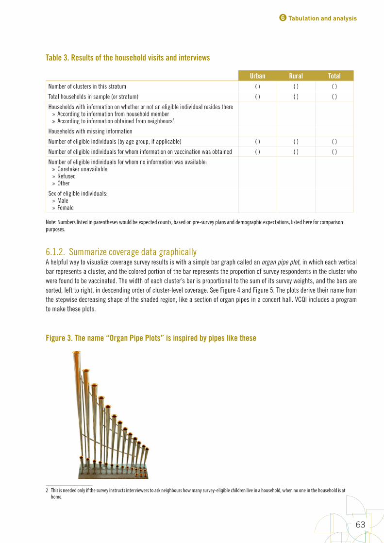
Table 3. Results of the household visits and interviews
Urban Rural TotalNumber of clusters in this stratum ( ) ( ) ( )
Total households in sample (or stratum) ( ) ( ) ( )
Households with information on whether or not an eligible individual resides there » According to information from household member » According to information obtained from neighbours2
Households with missing information
Number of eligible individuals (by age group, if applicable) ( ) ( ) ( )
Number of eligible individuals for whom information on vaccination was obtained ( ) ( ) ( )
Number of eligible individuals for whom no information was available: » Caretaker unavailable » Refused » Other
Sex of eligible individuals: » Male » Female
Note: Numbers listed in parentheses would be expected counts, based on pre-survey plans and demographic expectations, listed here for comparison purposes.2
6.1.2. Summarize coverage data graphically A helpful way to visualize coverage survey results is with a simple bar graph called an organ pipe plot, in which each vertical bar represents a cluster, and the colored portion of the bar represents the proportion of survey respondents in the cluster who were found to be vaccinated. The width of each cluster’s bar is proportional to the sum of its survey weights, and the bars are sorted, left to right, in descending order of cluster-level coverage. See Figure 4 and Figure 5. The plots derive their name from the stepwise decreasing shape of the shaded region, like a section of organ pipes in a concert hall. VCQI includes a program to make these plots.
2 This is needed only if the survey instructs interviewers to ask neighbours how many survey-eligible children live in a household, when no one in the household is at home.
Figure 3. The name “Organ Pipe Plots” is inspired by pipes like these
6 Tabulation and analysis
63
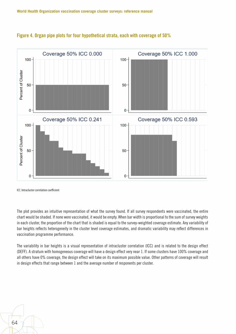
The plot provides an intuitive representation of what the survey found. If all survey respondents were vaccinated, the entire chart would be shaded. If none were vaccinated, it would be empty. When bar width is proportional to the sum of survey weights in each cluster, the proportion of the chart that is shaded is equal to the survey-weighted coverage estimate. Any variability of bar heights reflects heterogeneity in the cluster level coverage estimates, and dramatic variability may reflect differences in vaccination programme performance.
The variability in bar heights is a visual representation of intracluster correlation (ICC) and is related to the design effect (DEFF). A stratum with homogeneous coverage will have a design effect very near 1. If some clusters have 100% coverage and all others have 0% coverage, the design effect will take on its maximum possible value. Other patterns of coverage will result in design effects that range between 1 and the average number of responents per cluster.
Figure 4. Organ pipe plots for four hypothetical strata, each with coverage of 50%
ICC: Intracluster correlation coefficient
World Health Organization vaccination coverage cluster surveys: reference manual
64
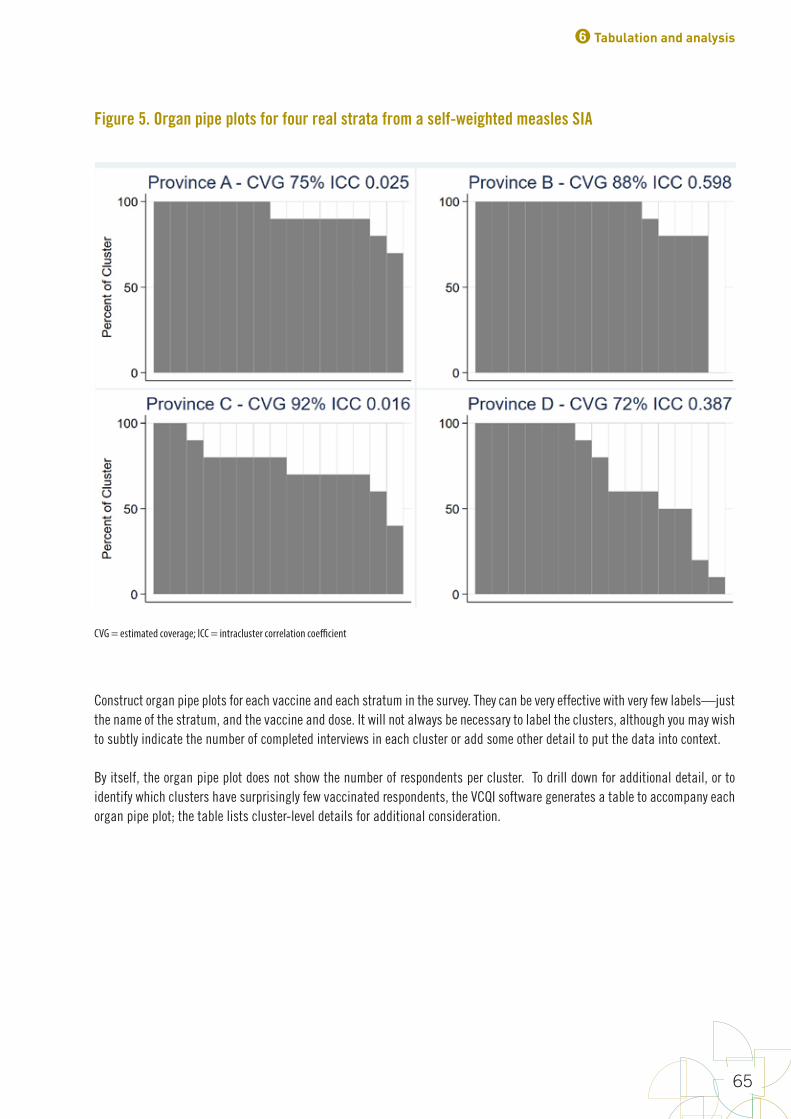
Construct organ pipe plots for each vaccine and each stratum in the survey. They can be very effective with very few labels—just the name of the stratum, and the vaccine and dose. It will not always be necessary to label the clusters, although you may wish to subtly indicate the number of completed interviews in each cluster or add some other detail to put the data into context.
By itself, the organ pipe plot does not show the number of respondents per cluster. To drill down for additional detail, or to identify which clusters have surprisingly few vaccinated respondents, the VCQI software generates a table to accompany each organ pipe plot; the table lists cluster-level details for additional consideration.
Figure 5. Organ pipe plots for four real strata from a self-weighted measles SIA
CVG = estimated coverage; ICC = intracluster correlation coefficient
6 Tabulation and analysis
65
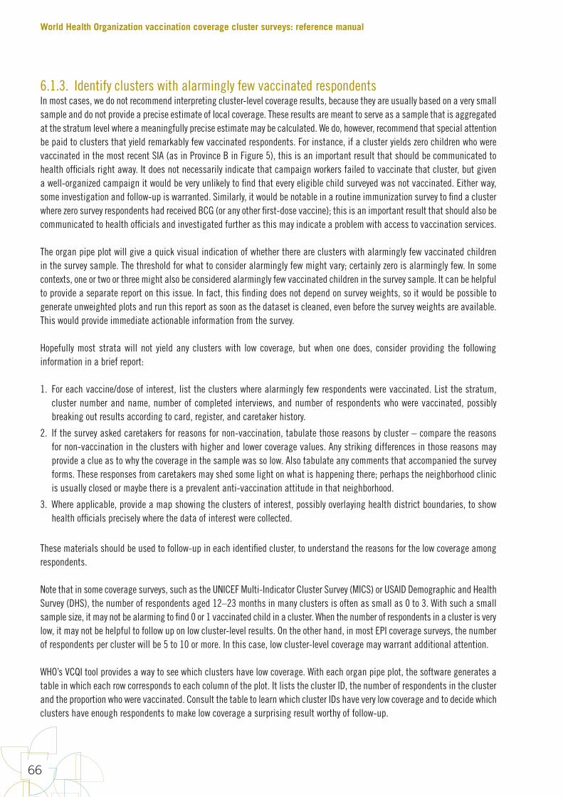
6.1.3. Identify clusters with alarmingly few vaccinated respondentsIn most cases, we do not recommend interpreting cluster-level coverage results, because they are usually based on a very small sample and do not provide a precise estimate of local coverage. These results are meant to serve as a sample that is aggregated at the stratum level where a meaningfully precise estimate may be calculated. We do, however, recommend that special attention be paid to clusters that yield remarkably few vaccinated respondents. For instance, if a cluster yields zero children who were vaccinated in the most recent SIA (as in Province B in Figure 5), this is an important result that should be communicated to health officials right away. It does not necessarily indicate that campaign workers failed to vaccinate that cluster, but given a well-organized campaign it would be very unlikely to find that every eligible child surveyed was not vaccinated. Either way, some investigation and follow-up is warranted. Similarly, it would be notable in a routine immunization survey to find a cluster where zero survey respondents had received BCG (or any other first-dose vaccine); this is an important result that should also be communicated to health officials and investigated further as this may indicate a problem with access to vaccination services.
The organ pipe plot will give a quick visual indication of whether there are clusters with alarmingly few vaccinated children in the survey sample. The threshold for what to consider alarmingly few might vary; certainly zero is alarmingly few. In some contexts, one or two or three might also be considered alarmingly few vaccinated children in the survey sample. It can be helpful to provide a separate report on this issue. In fact, this finding does not depend on survey weights, so it would be possible to generate unweighted plots and run this report as soon as the dataset is cleaned, even before the survey weights are available. This would provide immediate actionable information from the survey.
Hopefully most strata will not yield any clusters with low coverage, but when one does, consider providing the following information in a brief report:
1. For each vaccine/dose of interest, list the clusters where alarmingly few respondents were vaccinated. List the stratum, cluster number and name, number of completed interviews, and number of respondents who were vaccinated, possibly breaking out results according to card, register, and caretaker history.
2. If the survey asked caretakers for reasons for non-vaccination, tabulate those reasons by cluster – compare the reasons for non-vaccination in the clusters with higher and lower coverage values. Any striking differences in those reasons may provide a clue as to why the coverage in the sample was so low. Also tabulate any comments that accompanied the survey forms. These responses from caretakers may shed some light on what is happening there; perhaps the neighborhood clinic is usually closed or maybe there is a prevalent anti-vaccination attitude in that neighborhood.
3. Where applicable, provide a map showing the clusters of interest, possibly overlaying health district boundaries, to show health officials precisely where the data of interest were collected.
These materials should be used to follow-up in each identified cluster, to understand the reasons for the low coverage among respondents.
Note that in some coverage surveys, such as the UNICEF Multi-Indicator Cluster Survey (MICS) or USAID Demographic and Health Survey (DHS), the number of respondents aged 12–23 months in many clusters is often as small as 0 to 3. With such a small sample size, it may not be alarming to find 0 or 1 vaccinated child in a cluster. When the number of respondents in a cluster is very low, it may not be helpful to follow up on low cluster-level results. On the other hand, in most EPI coverage surveys, the number of respondents per cluster will be 5 to 10 or more. In this case, low cluster-level coverage may warrant additional attention.
WHO’s VCQI tool provides a way to see which clusters have low coverage. With each organ pipe plot, the software generates a table in which each row corresponds to each column of the plot. It lists the cluster ID, the number of respondents in the cluster and the proportion who were vaccinated. Consult the table to learn which cluster IDs have very low coverage and to decide which clusters have enough respondents to make low coverage a surprising result worthy of follow-up.
World Health Organization vaccination coverage cluster surveys: reference manual
66
6.2. Calculate weights for analysisUnder the multistage PPES sampling approach described in this manual, the analysis will most likely need to be weighted because sampling probabilities will likely differ for different respondents. Each respondent’s data record will be accompanied by one or more weights that will be calculated by a statistician or partners in the national census agency. Weights can be scaled so they sum to the target population for the survey, in which case the weight is interpreted as the number of eligible respondents in the population who are represented by this respondent in the sample. The survey report should include an annex that clearly describes how the weights were calculated for your survey.
The calculation of sampling weights can be conducted in three steps: 1) calculating the design weight, 2) adjusting for nonresponse and 3) post-stratifying to match population totals. The first step should be done in all vaccination coverage surveys. The other two are applied as needed. Below is a description of how to calculate the sampling weights. The process is described in more detail in Annex J.
6.2.1. Calculate the design weightThe design weight is the reciprocal of the probability that the respondent was selected to participate in the survey, which is the product of the probabilities of selection at each stage. There can commonly be up to four stages of selection:
1.
76
neighborhoodclinicisusuallyclosedormaybethereisaprevalentanti-vaccinationattitudeinthatneighborhood.
3. Whereapplicable,provideamapshowingtheclustersofinterest,possiblyoverlayinghealthdistrictboundaries,toshowhealthofficialspreciselywherethedataofinterestwerecollected.
Thesematerialsshouldbeusedtofollow-upforineachidentifiedcluster,tounderstandthereasonsforthelowcoverageamongrespondents.
Notethatinsomecoveragesurveys,suchastheUNICEFMulti-IndicatorClusterSurvey(MICS)orDemographicandHealthSurvey(DHS),thenumberofrespondentsaged12–23monthsinmanyclustersisoftenassmallas0to3.Withsuchasmallsamplesize,itmaynotbealarmingtofind0or1vaccinatedchildinacluster.Whenthenumberofrespondentsinaclusterisverylow,itmaynotbehelpfultofollowuponlowcluster-levelresults.Ontheotherhand,inmostEPIcoveragesurveys,thenumberofrespondentsperclusterwillbe5to10ormore.Inthiscase,lowcluster-levelcoveragemaywarrantadditionalattention.
WHO’sVCQIsoftwareprovidesawaytoseewhichclustershavelowcoverage.Witheachorganpipeplot,thesoftwaregeneratesatableinwhicheachrowcorrespondstoeachcolumnoftheplot.ItliststheclusterID,thenumberofrespondentsintheclusterandtheproportionwhowerevaccinated.ConsultthetabletolearnwhichclusterIDshaveverylowcoverageandtodecidewhichclustershaveenoughrespondentstomakelowcoverageasurprisingresultworthyoffollow-up.
6.2. Calculate weights for analysis UnderthemultistagePPESsamplingapproachdescribedinthismanual,theanalysiswillmostlikelyneedtobeweightedbecausesamplingprobabilitieswilllikelydifferfordifferentrespondents.Eachrespondent’sdatarecordwillbeaccompaniedbyoneormoreweightsthatwillbecalculatedbyastatisticianorpartnersinthenationalcensusagency.Weightscanbescaledsotheysumtothetargetpopulationforthesurvey,inwhichcasetheweightisinterpretedasthenumberofeligiblerespondentsinthepopulationwhoarerepresentedbythisrespondentinthesample.Thesurveyreportshouldincludeanannexthatclearlydescribeshowtheweightswerecalculatedforyoursurvey.
Thecalculationofsamplingweightscanbeconductedinthreesteps:1)calculatingthedesignweight,2)adjustingfornonresponseand3)post-stratifyingtomatchpopulationtotals.Thefirststepshouldbedoneinallvaccinationcoveragesurveys.Theothertwoareappliedasneeded.Belowisadescriptionofhowtocalculatethesamplingweights.TheprocessisdescribedinmoredetailinAnnexJ.
6.2.1. Calculate the design weight Thedesignweightisthereciprocaloftheprobabilitythattherespondentwasselectedtoparticipateinthesurvey,whichistheproductoftheprobabilitiesofselectionateachstage.Therecancommonlybeuptofourstagesofselection:
1. 𝑝𝑝456istheprobabilitythatthePSUwasselectedfromtheframeofallpossiblePSUs2. 𝑝𝑝578%79:;9456istheprobabilitythatthesegmentofthePSUwasselectedfromthelistof
segmentsinthePSU(=1ifthePSUisnotsegmented)
is the probability that the PSU was selected from the frame of all possible PSUs
2.
76
neighborhoodclinicisusuallyclosedormaybethereisaprevalentanti-vaccinationattitudeinthatneighborhood.
3. Whereapplicable,provideamapshowingtheclustersofinterest,possiblyoverlayinghealthdistrictboundaries,toshowhealthofficialspreciselywherethedataofinterestwerecollected.
Thesematerialsshouldbeusedtofollow-upforineachidentifiedcluster,tounderstandthereasonsforthelowcoverageamongrespondents.
Notethatinsomecoveragesurveys,suchastheUNICEFMulti-IndicatorClusterSurvey(MICS)orDemographicandHealthSurvey(DHS),thenumberofrespondentsaged12–23monthsinmanyclustersisoftenassmallas0to3.Withsuchasmallsamplesize,itmaynotbealarmingtofind0or1vaccinatedchildinacluster.Whenthenumberofrespondentsinaclusterisverylow,itmaynotbehelpfultofollowuponlowcluster-levelresults.Ontheotherhand,inmostEPIcoveragesurveys,thenumberofrespondentsperclusterwillbe5to10ormore.Inthiscase,lowcluster-levelcoveragemaywarrantadditionalattention.
WHO’sVCQIsoftwareprovidesawaytoseewhichclustershavelowcoverage.Witheachorganpipeplot,thesoftwaregeneratesatableinwhicheachrowcorrespondstoeachcolumnoftheplot.ItliststheclusterID,thenumberofrespondentsintheclusterandtheproportionwhowerevaccinated.ConsultthetabletolearnwhichclusterIDshaveverylowcoverageandtodecidewhichclustershaveenoughrespondentstomakelowcoverageasurprisingresultworthyoffollow-up.
6.2. Calculate weights for analysis UnderthemultistagePPESsamplingapproachdescribedinthismanual,theanalysiswillmostlikelyneedtobeweightedbecausesamplingprobabilitieswilllikelydifferfordifferentrespondents.Eachrespondent’sdatarecordwillbeaccompaniedbyoneormoreweightsthatwillbecalculatedbyastatisticianorpartnersinthenationalcensusagency.Weightscanbescaledsotheysumtothetargetpopulationforthesurvey,inwhichcasetheweightisinterpretedasthenumberofeligiblerespondentsinthepopulationwhoarerepresentedbythisrespondentinthesample.Thesurveyreportshouldincludeanannexthatclearlydescribeshowtheweightswerecalculatedforyoursurvey.
Thecalculationofsamplingweightscanbeconductedinthreesteps:1)calculatingthedesignweight,2)adjustingfornonresponseand3)post-stratifyingtomatchpopulationtotals.Thefirststepshouldbedoneinallvaccinationcoveragesurveys.Theothertwoareappliedasneeded.Belowisadescriptionofhowtocalculatethesamplingweights.TheprocessisdescribedinmoredetailinAnnexJ.
6.2.1. Calculate the design weight Thedesignweightisthereciprocaloftheprobabilitythattherespondentwasselectedtoparticipateinthesurvey,whichistheproductoftheprobabilitiesofselectionateachstage.Therecancommonlybeuptofourstagesofselection:
1. 𝑝𝑝456istheprobabilitythatthePSUwasselectedfromtheframeofallpossiblePSUs2. 𝑝𝑝578%79:;9456istheprobabilitythatthesegmentofthePSUwasselectedfromthelistof
segmentsinthePSU(=1ifthePSUisnotsegmented) is the probability that the segment of the PSU was selected from the list of segments in the PSU (equals
1 if the PSU is not segmented)
3.
77
3. 𝑝𝑝<=>?7@=AB;9578%79:istheprobabilitythatthehouseholdwasselectedfromthelistofhouseholdsinthesegment(=1ifallhouseholdsareselected)
4. 𝑝𝑝C7?D=9B79:;9<=>?7@=ABistheprobabilitythattherespondentwasselectedfromthelistofeligiblerespondentsinthehousehold(=1ifallrespondentsareselected)
Theprobabilitythattherespondentisselectedis
𝑝𝑝57A7E:;=9 = 𝑝𝑝456 ∗ 𝑝𝑝578%79:;9456 ∗ 𝑝𝑝<=>?7@=AB;9578%79: ∗ 𝑝𝑝C7?D=9B79:;9<=>?7@=AB
Thedesignweightis:
𝑊𝑊𝑊𝑊𝑊𝑊𝑊𝑊ℎ𝑡𝑡N7?;89 =1
𝑃𝑃57A7E:;=9
6.2.2. Adjust for nonresponse Thedesignweightreflectstheselectionprocess,andallthesampledeligiblepersonswillhaveapositivevaluefor𝑊𝑊𝑊𝑊𝑊𝑊𝑊𝑊ℎ𝑡𝑡N7?;89.However,itwillnotbepossibletoobtaininformationonalltheselectedrespondents,forexample,becausethecaretakersareabsentorrefusetoparticipateinthesurvey.Toensurethatthesurveyresultsrepresentthetargetpopulation,anadjustmentismadetothedesignweighttotransferthesamplingweightofthenon-respondentstotherespondentsofthesurvey.Thisadjustmentisreferredtoasthenonresponseadjustment.Thenonresponseadjustmentshouldbedonebyasurveystatistician.
Therearenumerouswaystodoanonresponseadjustment.Sophisticatedadjustmentsrequirecollectingauxiliaryinformationavailableforboththerespondentsandthenon-respondents.InthecontextoftheEPIsurveys,thesamplingframesandthehousehold-levelinformationareusuallyverylimitedanddonotpermitforthesesophisticatednonresponseadjustmentmethods.Furthermore,thegenerallyhighresponseratesintheEPIsurveysdonotsuggestimportantdifferencesinresponseratebetweengroups.
Hence,fortheEPIsurveys,doanon-responseadjustmentbyformingadjustmentclasseswithineachstratum,andadjustingthedesignweightwithinthoseclasses.Ifmorethanoneagecohortwassurveyed,agecohortswithinstratumcanbeusedastheresponseclasses.Itmayalsomakesensetouseadministrativelevelssuchasdistrictstoformtheresponseclasses.Ifimplicitstratificationwasusedtoselectthesample,thecorrespondingvariablecanbethebasisforformingnonresponseclasses.Forexample,ifresidencetype(urban/rural)wasusedasimplicitstratification,thenseparateurbanandruralnonresponseclassescanbeusedfortheweightadjustment.Infact,itmaymakesensetosystematicallyuseresidencetypetoformthenonresponseclassesregardlessofituseintheselectionprocess.
Withineachnonresponseclass,calculatethenonresponseadjustmentfactor(𝑎𝑎𝑎𝑎𝑎𝑎TC)astheratioofthesumofallthedesignweightsintheclasstothesumofthedesignweightsoftherespondents.Obtaintheresponseweight(𝑊𝑊𝑊𝑊𝑊𝑊𝑊𝑊ℎ𝑡𝑡C7?D=9?7)bymultiplyingthedesignweightoftherespondentbytheadjustmentfactorthatis𝑊𝑊𝑊𝑊𝑊𝑊𝑊𝑊ℎ𝑡𝑡C7?D=9?7 = 𝑎𝑎𝑎𝑎𝑎𝑎TC ∗ 𝑊𝑊𝑊𝑊𝑊𝑊𝑊𝑊ℎ𝑡𝑡N7?;89.Notethatthenon-respondentswillbegivenaweightof0andexcludedfromthefinalanalysisfile.
is the probability that the household was selected from the list of households in the segment (equals 1 if all households are selected)
4.
77
3. 𝑝𝑝<=>?7@=AB;9578%79:istheprobabilitythatthehouseholdwasselectedfromthelistofhouseholdsinthesegment(=1ifallhouseholdsareselected)
4. 𝑝𝑝C7?D=9B79:;9<=>?7@=ABistheprobabilitythattherespondentwasselectedfromthelistofeligiblerespondentsinthehousehold(=1ifallrespondentsareselected)
Theprobabilitythattherespondentisselectedis
𝑝𝑝57A7E:;=9 = 𝑝𝑝456 ∗ 𝑝𝑝578%79:;9456 ∗ 𝑝𝑝<=>?7@=AB;9578%79: ∗ 𝑝𝑝C7?D=9B79:;9<=>?7@=AB
Thedesignweightis:
𝑊𝑊𝑊𝑊𝑊𝑊𝑊𝑊ℎ𝑡𝑡N7?;89 =1
𝑃𝑃57A7E:;=9
6.2.2. Adjust for nonresponse Thedesignweightreflectstheselectionprocess,andallthesampledeligiblepersonswillhaveapositivevaluefor𝑊𝑊𝑊𝑊𝑊𝑊𝑊𝑊ℎ𝑡𝑡N7?;89.However,itwillnotbepossibletoobtaininformationonalltheselectedrespondents,forexample,becausethecaretakersareabsentorrefusetoparticipateinthesurvey.Toensurethatthesurveyresultsrepresentthetargetpopulation,anadjustmentismadetothedesignweighttotransferthesamplingweightofthenon-respondentstotherespondentsofthesurvey.Thisadjustmentisreferredtoasthenonresponseadjustment.Thenonresponseadjustmentshouldbedonebyasurveystatistician.
Therearenumerouswaystodoanonresponseadjustment.Sophisticatedadjustmentsrequirecollectingauxiliaryinformationavailableforboththerespondentsandthenon-respondents.InthecontextoftheEPIsurveys,thesamplingframesandthehousehold-levelinformationareusuallyverylimitedanddonotpermitforthesesophisticatednonresponseadjustmentmethods.Furthermore,thegenerallyhighresponseratesintheEPIsurveysdonotsuggestimportantdifferencesinresponseratebetweengroups.
Hence,fortheEPIsurveys,doanon-responseadjustmentbyformingadjustmentclasseswithineachstratum,andadjustingthedesignweightwithinthoseclasses.Ifmorethanoneagecohortwassurveyed,agecohortswithinstratumcanbeusedastheresponseclasses.Itmayalsomakesensetouseadministrativelevelssuchasdistrictstoformtheresponseclasses.Ifimplicitstratificationwasusedtoselectthesample,thecorrespondingvariablecanbethebasisforformingnonresponseclasses.Forexample,ifresidencetype(urban/rural)wasusedasimplicitstratification,thenseparateurbanandruralnonresponseclassescanbeusedfortheweightadjustment.Infact,itmaymakesensetosystematicallyuseresidencetypetoformthenonresponseclassesregardlessofituseintheselectionprocess.
Withineachnonresponseclass,calculatethenonresponseadjustmentfactor(𝑎𝑎𝑎𝑎𝑎𝑎TC)astheratioofthesumofallthedesignweightsintheclasstothesumofthedesignweightsoftherespondents.Obtaintheresponseweight(𝑊𝑊𝑊𝑊𝑊𝑊𝑊𝑊ℎ𝑡𝑡C7?D=9?7)bymultiplyingthedesignweightoftherespondentbytheadjustmentfactorthatis𝑊𝑊𝑊𝑊𝑊𝑊𝑊𝑊ℎ𝑡𝑡C7?D=9?7 = 𝑎𝑎𝑎𝑎𝑎𝑎TC ∗ 𝑊𝑊𝑊𝑊𝑊𝑊𝑊𝑊ℎ𝑡𝑡N7?;89.Notethatthenon-respondentswillbegivenaweightof0andexcludedfromthefinalanalysisfile.
is the probability that the respondent was selected from the list of eligible respondents in the household (equals 1 if all respondents are selected)
The probability that the respondent is selected is
77
3. 𝑝𝑝<=>?7@=AB;9578%79:istheprobabilitythatthehouseholdwasselectedfromthelistofhouseholdsinthesegment(=1ifallhouseholdsareselected)
4. 𝑝𝑝C7?D=9B79:;9<=>?7@=ABistheprobabilitythattherespondentwasselectedfromthelistofeligiblerespondentsinthehousehold(=1ifallrespondentsareselected)
Theprobabilitythattherespondentisselectedis
𝑝𝑝57A7E:;=9 = 𝑝𝑝456 ∗ 𝑝𝑝578%79:;9456 ∗ 𝑝𝑝<=>?7@=AB;9578%79: ∗ 𝑝𝑝C7?D=9B79:;9<=>?7@=AB
Thedesignweightis:
𝑊𝑊𝑊𝑊𝑊𝑊𝑊𝑊ℎ𝑡𝑡N7?;89 =1
𝑃𝑃57A7E:;=9
6.2.2. Adjust for nonresponse Thedesignweightreflectstheselectionprocess,andallthesampledeligiblepersonswillhaveapositivevaluefor𝑊𝑊𝑊𝑊𝑊𝑊𝑊𝑊ℎ𝑡𝑡N7?;89.However,itwillnotbepossibletoobtaininformationonalltheselectedrespondents,forexample,becausethecaretakersareabsentorrefusetoparticipateinthesurvey.Toensurethatthesurveyresultsrepresentthetargetpopulation,anadjustmentismadetothedesignweighttotransferthesamplingweightofthenon-respondentstotherespondentsofthesurvey.Thisadjustmentisreferredtoasthenonresponseadjustment.Thenonresponseadjustmentshouldbedonebyasurveystatistician.
Therearenumerouswaystodoanonresponseadjustment.Sophisticatedadjustmentsrequirecollectingauxiliaryinformationavailableforboththerespondentsandthenon-respondents.InthecontextoftheEPIsurveys,thesamplingframesandthehousehold-levelinformationareusuallyverylimitedanddonotpermitforthesesophisticatednonresponseadjustmentmethods.Furthermore,thegenerallyhighresponseratesintheEPIsurveysdonotsuggestimportantdifferencesinresponseratebetweengroups.
Hence,fortheEPIsurveys,doanon-responseadjustmentbyformingadjustmentclasseswithineachstratum,andadjustingthedesignweightwithinthoseclasses.Ifmorethanoneagecohortwassurveyed,agecohortswithinstratumcanbeusedastheresponseclasses.Itmayalsomakesensetouseadministrativelevelssuchasdistrictstoformtheresponseclasses.Ifimplicitstratificationwasusedtoselectthesample,thecorrespondingvariablecanbethebasisforformingnonresponseclasses.Forexample,ifresidencetype(urban/rural)wasusedasimplicitstratification,thenseparateurbanandruralnonresponseclassescanbeusedfortheweightadjustment.Infact,itmaymakesensetosystematicallyuseresidencetypetoformthenonresponseclassesregardlessofituseintheselectionprocess.
Withineachnonresponseclass,calculatethenonresponseadjustmentfactor(𝑎𝑎𝑎𝑎𝑎𝑎TC)astheratioofthesumofallthedesignweightsintheclasstothesumofthedesignweightsoftherespondents.Obtaintheresponseweight(𝑊𝑊𝑊𝑊𝑊𝑊𝑊𝑊ℎ𝑡𝑡C7?D=9?7)bymultiplyingthedesignweightoftherespondentbytheadjustmentfactorthatis𝑊𝑊𝑊𝑊𝑊𝑊𝑊𝑊ℎ𝑡𝑡C7?D=9?7 = 𝑎𝑎𝑎𝑎𝑎𝑎TC ∗ 𝑊𝑊𝑊𝑊𝑊𝑊𝑊𝑊ℎ𝑡𝑡N7?;89.Notethatthenon-respondentswillbegivenaweightof0andexcludedfromthefinalanalysisfile.
The design weight is:
77
3. 𝑝𝑝<=>?7@=AB;9578%79:istheprobabilitythatthehouseholdwasselectedfromthelistofhouseholdsinthesegment(=1ifallhouseholdsareselected)
4. 𝑝𝑝C7?D=9B79:;9<=>?7@=ABistheprobabilitythattherespondentwasselectedfromthelistofeligiblerespondentsinthehousehold(=1ifallrespondentsareselected)
Theprobabilitythattherespondentisselectedis
𝑝𝑝57A7E:;=9 = 𝑝𝑝456 ∗ 𝑝𝑝578%79:;9456 ∗ 𝑝𝑝<=>?7@=AB;9578%79: ∗ 𝑝𝑝C7?D=9B79:;9<=>?7@=AB
Thedesignweightis:
𝑊𝑊𝑊𝑊𝑊𝑊𝑊𝑊ℎ𝑡𝑡N7?;89 =1
𝑃𝑃57A7E:;=9
6.2.2. Adjust for nonresponse Thedesignweightreflectstheselectionprocess,andallthesampledeligiblepersonswillhaveapositivevaluefor𝑊𝑊𝑊𝑊𝑊𝑊𝑊𝑊ℎ𝑡𝑡N7?;89.However,itwillnotbepossibletoobtaininformationonalltheselectedrespondents,forexample,becausethecaretakersareabsentorrefusetoparticipateinthesurvey.Toensurethatthesurveyresultsrepresentthetargetpopulation,anadjustmentismadetothedesignweighttotransferthesamplingweightofthenon-respondentstotherespondentsofthesurvey.Thisadjustmentisreferredtoasthenonresponseadjustment.Thenonresponseadjustmentshouldbedonebyasurveystatistician.
Therearenumerouswaystodoanonresponseadjustment.Sophisticatedadjustmentsrequirecollectingauxiliaryinformationavailableforboththerespondentsandthenon-respondents.InthecontextoftheEPIsurveys,thesamplingframesandthehousehold-levelinformationareusuallyverylimitedanddonotpermitforthesesophisticatednonresponseadjustmentmethods.Furthermore,thegenerallyhighresponseratesintheEPIsurveysdonotsuggestimportantdifferencesinresponseratebetweengroups.
Hence,fortheEPIsurveys,doanon-responseadjustmentbyformingadjustmentclasseswithineachstratum,andadjustingthedesignweightwithinthoseclasses.Ifmorethanoneagecohortwassurveyed,agecohortswithinstratumcanbeusedastheresponseclasses.Itmayalsomakesensetouseadministrativelevelssuchasdistrictstoformtheresponseclasses.Ifimplicitstratificationwasusedtoselectthesample,thecorrespondingvariablecanbethebasisforformingnonresponseclasses.Forexample,ifresidencetype(urban/rural)wasusedasimplicitstratification,thenseparateurbanandruralnonresponseclassescanbeusedfortheweightadjustment.Infact,itmaymakesensetosystematicallyuseresidencetypetoformthenonresponseclassesregardlessofituseintheselectionprocess.
Withineachnonresponseclass,calculatethenonresponseadjustmentfactor(𝑎𝑎𝑎𝑎𝑎𝑎TC)astheratioofthesumofallthedesignweightsintheclasstothesumofthedesignweightsoftherespondents.Obtaintheresponseweight(𝑊𝑊𝑊𝑊𝑊𝑊𝑊𝑊ℎ𝑡𝑡C7?D=9?7)bymultiplyingthedesignweightoftherespondentbytheadjustmentfactorthatis𝑊𝑊𝑊𝑊𝑊𝑊𝑊𝑊ℎ𝑡𝑡C7?D=9?7 = 𝑎𝑎𝑎𝑎𝑎𝑎TC ∗ 𝑊𝑊𝑊𝑊𝑊𝑊𝑊𝑊ℎ𝑡𝑡N7?;89.Notethatthenon-respondentswillbegivenaweightof0andexcludedfromthefinalanalysisfile.
6.2.2. Adjust for nonresponseThe design weight reflects the selection process, and all the sampled eligible persons will have a positive value for
77
3. 𝑝𝑝<=>?7@=AB;9578%79:istheprobabilitythatthehouseholdwasselectedfromthelistofhouseholdsinthesegment(=1ifallhouseholdsareselected)
4. 𝑝𝑝C7?D=9B79:;9<=>?7@=ABistheprobabilitythattherespondentwasselectedfromthelistofeligiblerespondentsinthehousehold(=1ifallrespondentsareselected)
Theprobabilitythattherespondentisselectedis
𝑝𝑝57A7E:;=9 = 𝑝𝑝456 ∗ 𝑝𝑝578%79:;9456 ∗ 𝑝𝑝<=>?7@=AB;9578%79: ∗ 𝑝𝑝C7?D=9B79:;9<=>?7@=AB
Thedesignweightis:
𝑊𝑊𝑊𝑊𝑊𝑊𝑊𝑊ℎ𝑡𝑡N7?;89 =1
𝑃𝑃57A7E:;=9
6.2.2. Adjust for nonresponse Thedesignweightreflectstheselectionprocess,andallthesampledeligiblepersonswillhaveapositivevaluefor𝑊𝑊𝑊𝑊𝑊𝑊𝑊𝑊ℎ𝑡𝑡N7?;89.However,itwillnotbepossibletoobtaininformationonalltheselectedrespondents,forexample,becausethecaretakersareabsentorrefusetoparticipateinthesurvey.Toensurethatthesurveyresultsrepresentthetargetpopulation,anadjustmentismadetothedesignweighttotransferthesamplingweightofthenon-respondentstotherespondentsofthesurvey.Thisadjustmentisreferredtoasthenonresponseadjustment.Thenonresponseadjustmentshouldbedonebyasurveystatistician.
Therearenumerouswaystodoanonresponseadjustment.Sophisticatedadjustmentsrequirecollectingauxiliaryinformationavailableforboththerespondentsandthenon-respondents.InthecontextoftheEPIsurveys,thesamplingframesandthehousehold-levelinformationareusuallyverylimitedanddonotpermitforthesesophisticatednonresponseadjustmentmethods.Furthermore,thegenerallyhighresponseratesintheEPIsurveysdonotsuggestimportantdifferencesinresponseratebetweengroups.
Hence,fortheEPIsurveys,doanon-responseadjustmentbyformingadjustmentclasseswithineachstratum,andadjustingthedesignweightwithinthoseclasses.Ifmorethanoneagecohortwassurveyed,agecohortswithinstratumcanbeusedastheresponseclasses.Itmayalsomakesensetouseadministrativelevelssuchasdistrictstoformtheresponseclasses.Ifimplicitstratificationwasusedtoselectthesample,thecorrespondingvariablecanbethebasisforformingnonresponseclasses.Forexample,ifresidencetype(urban/rural)wasusedasimplicitstratification,thenseparateurbanandruralnonresponseclassescanbeusedfortheweightadjustment.Infact,itmaymakesensetosystematicallyuseresidencetypetoformthenonresponseclassesregardlessofituseintheselectionprocess.
Withineachnonresponseclass,calculatethenonresponseadjustmentfactor(𝑎𝑎𝑎𝑎𝑎𝑎TC)astheratioofthesumofallthedesignweightsintheclasstothesumofthedesignweightsoftherespondents.Obtaintheresponseweight(𝑊𝑊𝑊𝑊𝑊𝑊𝑊𝑊ℎ𝑡𝑡C7?D=9?7)bymultiplyingthedesignweightoftherespondentbytheadjustmentfactorthatis𝑊𝑊𝑊𝑊𝑊𝑊𝑊𝑊ℎ𝑡𝑡C7?D=9?7 = 𝑎𝑎𝑎𝑎𝑎𝑎TC ∗ 𝑊𝑊𝑊𝑊𝑊𝑊𝑊𝑊ℎ𝑡𝑡N7?;89.Notethatthenon-respondentswillbegivenaweightof0andexcludedfromthefinalanalysisfile.
However, it will not be possible to obtain information on all the selected respondents, for example, because the caretakers are absent or refuse to participate in the survey. To ensure that the survey results represent the target population, an adjustment is made to the design weight to transfer the sampling weight of the non-respondents to the respondents of the survey. This adjustment is referred to as the nonresponse adjustment. The nonresponse adjustment should be done by a survey statistician.
There are numerous ways to do a nonresponse adjustment. Sophisticated adjustments require collecting auxiliary information available for both the respondents and the non-respondents. In the context of the EPI surveys, the sampling frames and the household-level information are usually very limited and do not permit for these sophisticated nonresponse adjustment methods. Furthermore, the generally high response rates in the EPI surveys do not suggest important differences in response rates between groups.
6 Tabulation and analysis
67
Hence, for the EPI surveys, do a non-response adjustment by forming adjustment classes within each stratum, and adjusting the design weight within those classes. If more than one age cohort was surveyed, age cohorts within stratum can be used as the response classes. It may also make sense to use administrative levels such as districts to form the response classes. If implicit stratification was used to select the sample, the corresponding variable can be the basis for forming non-response classes. For example, if residence type (urban/rural) was used as implicit stratification, then separate urban and rural non-response classes can be used for the weight adjustment. In fact, it may make sense to systematically use residence type to form the non-response classes regardless of its use in the selection process.
Within each non-response class, calculate the non-response adjustment factor
77
3. 𝑝𝑝<=>?7@=AB;9578%79:istheprobabilitythatthehouseholdwasselectedfromthelistofhouseholdsinthesegment(=1ifallhouseholdsareselected)
4. 𝑝𝑝C7?D=9B79:;9<=>?7@=ABistheprobabilitythattherespondentwasselectedfromthelistofeligiblerespondentsinthehousehold(=1ifallrespondentsareselected)
Theprobabilitythattherespondentisselectedis
𝑝𝑝57A7E:;=9 = 𝑝𝑝456 ∗ 𝑝𝑝578%79:;9456 ∗ 𝑝𝑝<=>?7@=AB;9578%79: ∗ 𝑝𝑝C7?D=9B79:;9<=>?7@=AB
Thedesignweightis:
𝑊𝑊𝑊𝑊𝑊𝑊𝑊𝑊ℎ𝑡𝑡N7?;89 =1
𝑃𝑃57A7E:;=9
6.2.2. Adjust for nonresponse Thedesignweightreflectstheselectionprocess,andallthesampledeligiblepersonswillhaveapositivevaluefor𝑊𝑊𝑊𝑊𝑊𝑊𝑊𝑊ℎ𝑡𝑡N7?;89.However,itwillnotbepossibletoobtaininformationonalltheselectedrespondents,forexample,becausethecaretakersareabsentorrefusetoparticipateinthesurvey.Toensurethatthesurveyresultsrepresentthetargetpopulation,anadjustmentismadetothedesignweighttotransferthesamplingweightofthenon-respondentstotherespondentsofthesurvey.Thisadjustmentisreferredtoasthenonresponseadjustment.Thenonresponseadjustmentshouldbedonebyasurveystatistician.
Therearenumerouswaystodoanonresponseadjustment.Sophisticatedadjustmentsrequirecollectingauxiliaryinformationavailableforboththerespondentsandthenon-respondents.InthecontextoftheEPIsurveys,thesamplingframesandthehousehold-levelinformationareusuallyverylimitedanddonotpermitforthesesophisticatednonresponseadjustmentmethods.Furthermore,thegenerallyhighresponseratesintheEPIsurveysdonotsuggestimportantdifferencesinresponseratebetweengroups.
Hence,fortheEPIsurveys,doanon-responseadjustmentbyformingadjustmentclasseswithineachstratum,andadjustingthedesignweightwithinthoseclasses.Ifmorethanoneagecohortwassurveyed,agecohortswithinstratumcanbeusedastheresponseclasses.Itmayalsomakesensetouseadministrativelevelssuchasdistrictstoformtheresponseclasses.Ifimplicitstratificationwasusedtoselectthesample,thecorrespondingvariablecanbethebasisforformingnonresponseclasses.Forexample,ifresidencetype(urban/rural)wasusedasimplicitstratification,thenseparateurbanandruralnonresponseclassescanbeusedfortheweightadjustment.Infact,itmaymakesensetosystematicallyuseresidencetypetoformthenonresponseclassesregardlessofituseintheselectionprocess.
Withineachnonresponseclass,calculatethenonresponseadjustmentfactor(𝑎𝑎𝑎𝑎𝑎𝑎TC)astheratioofthesumofallthedesignweightsintheclasstothesumofthedesignweightsoftherespondents.Obtaintheresponseweight(𝑊𝑊𝑊𝑊𝑊𝑊𝑊𝑊ℎ𝑡𝑡C7?D=9?7)bymultiplyingthedesignweightoftherespondentbytheadjustmentfactorthatis𝑊𝑊𝑊𝑊𝑊𝑊𝑊𝑊ℎ𝑡𝑡C7?D=9?7 = 𝑎𝑎𝑎𝑎𝑎𝑎TC ∗ 𝑊𝑊𝑊𝑊𝑊𝑊𝑊𝑊ℎ𝑡𝑡N7?;89.Notethatthenon-respondentswillbegivenaweightof0andexcludedfromthefinalanalysisfile.
as the ratio of the sum of all the design weights in the class to the sum of the design weights of the respondents. Obtain the response weight
77
3. 𝑝𝑝<=>?7@=AB;9578%79:istheprobabilitythatthehouseholdwasselectedfromthelistofhouseholdsinthesegment(=1ifallhouseholdsareselected)
4. 𝑝𝑝C7?D=9B79:;9<=>?7@=ABistheprobabilitythattherespondentwasselectedfromthelistofeligiblerespondentsinthehousehold(=1ifallrespondentsareselected)
Theprobabilitythattherespondentisselectedis
𝑝𝑝57A7E:;=9 = 𝑝𝑝456 ∗ 𝑝𝑝578%79:;9456 ∗ 𝑝𝑝<=>?7@=AB;9578%79: ∗ 𝑝𝑝C7?D=9B79:;9<=>?7@=AB
Thedesignweightis:
𝑊𝑊𝑊𝑊𝑊𝑊𝑊𝑊ℎ𝑡𝑡N7?;89 =1
𝑃𝑃57A7E:;=9
6.2.2. Adjust for nonresponse Thedesignweightreflectstheselectionprocess,andallthesampledeligiblepersonswillhaveapositivevaluefor𝑊𝑊𝑊𝑊𝑊𝑊𝑊𝑊ℎ𝑡𝑡N7?;89.However,itwillnotbepossibletoobtaininformationonalltheselectedrespondents,forexample,becausethecaretakersareabsentorrefusetoparticipateinthesurvey.Toensurethatthesurveyresultsrepresentthetargetpopulation,anadjustmentismadetothedesignweighttotransferthesamplingweightofthenon-respondentstotherespondentsofthesurvey.Thisadjustmentisreferredtoasthenonresponseadjustment.Thenonresponseadjustmentshouldbedonebyasurveystatistician.
Therearenumerouswaystodoanonresponseadjustment.Sophisticatedadjustmentsrequirecollectingauxiliaryinformationavailableforboththerespondentsandthenon-respondents.InthecontextoftheEPIsurveys,thesamplingframesandthehousehold-levelinformationareusuallyverylimitedanddonotpermitforthesesophisticatednonresponseadjustmentmethods.Furthermore,thegenerallyhighresponseratesintheEPIsurveysdonotsuggestimportantdifferencesinresponseratebetweengroups.
Hence,fortheEPIsurveys,doanon-responseadjustmentbyformingadjustmentclasseswithineachstratum,andadjustingthedesignweightwithinthoseclasses.Ifmorethanoneagecohortwassurveyed,agecohortswithinstratumcanbeusedastheresponseclasses.Itmayalsomakesensetouseadministrativelevelssuchasdistrictstoformtheresponseclasses.Ifimplicitstratificationwasusedtoselectthesample,thecorrespondingvariablecanbethebasisforformingnonresponseclasses.Forexample,ifresidencetype(urban/rural)wasusedasimplicitstratification,thenseparateurbanandruralnonresponseclassescanbeusedfortheweightadjustment.Infact,itmaymakesensetosystematicallyuseresidencetypetoformthenonresponseclassesregardlessofituseintheselectionprocess.
Withineachnonresponseclass,calculatethenonresponseadjustmentfactor(𝑎𝑎𝑎𝑎𝑎𝑎TC)astheratioofthesumofallthedesignweightsintheclasstothesumofthedesignweightsoftherespondents.Obtaintheresponseweight(𝑊𝑊𝑊𝑊𝑊𝑊𝑊𝑊ℎ𝑡𝑡C7?D=9?7)bymultiplyingthedesignweightoftherespondentbytheadjustmentfactorthatis𝑊𝑊𝑊𝑊𝑊𝑊𝑊𝑊ℎ𝑡𝑡C7?D=9?7 = 𝑎𝑎𝑎𝑎𝑎𝑎TC ∗ 𝑊𝑊𝑊𝑊𝑊𝑊𝑊𝑊ℎ𝑡𝑡N7?;89.Notethatthenon-respondentswillbegivenaweightof0andexcludedfromthefinalanalysisfile.
by multiplying the design weight of the respondent by the adjustment factor that is
77
3. 𝑝𝑝<=>?7@=AB;9578%79:istheprobabilitythatthehouseholdwasselectedfromthelistofhouseholdsinthesegment(=1ifallhouseholdsareselected)
4. 𝑝𝑝C7?D=9B79:;9<=>?7@=ABistheprobabilitythattherespondentwasselectedfromthelistofeligiblerespondentsinthehousehold(=1ifallrespondentsareselected)
Theprobabilitythattherespondentisselectedis
𝑝𝑝57A7E:;=9 = 𝑝𝑝456 ∗ 𝑝𝑝578%79:;9456 ∗ 𝑝𝑝<=>?7@=AB;9578%79: ∗ 𝑝𝑝C7?D=9B79:;9<=>?7@=AB
Thedesignweightis:
𝑊𝑊𝑊𝑊𝑊𝑊𝑊𝑊ℎ𝑡𝑡N7?;89 =1
𝑃𝑃57A7E:;=9
6.2.2. Adjust for nonresponse Thedesignweightreflectstheselectionprocess,andallthesampledeligiblepersonswillhaveapositivevaluefor𝑊𝑊𝑊𝑊𝑊𝑊𝑊𝑊ℎ𝑡𝑡N7?;89.However,itwillnotbepossibletoobtaininformationonalltheselectedrespondents,forexample,becausethecaretakersareabsentorrefusetoparticipateinthesurvey.Toensurethatthesurveyresultsrepresentthetargetpopulation,anadjustmentismadetothedesignweighttotransferthesamplingweightofthenon-respondentstotherespondentsofthesurvey.Thisadjustmentisreferredtoasthenonresponseadjustment.Thenonresponseadjustmentshouldbedonebyasurveystatistician.
Therearenumerouswaystodoanonresponseadjustment.Sophisticatedadjustmentsrequirecollectingauxiliaryinformationavailableforboththerespondentsandthenon-respondents.InthecontextoftheEPIsurveys,thesamplingframesandthehousehold-levelinformationareusuallyverylimitedanddonotpermitforthesesophisticatednonresponseadjustmentmethods.Furthermore,thegenerallyhighresponseratesintheEPIsurveysdonotsuggestimportantdifferencesinresponseratebetweengroups.
Hence,fortheEPIsurveys,doanon-responseadjustmentbyformingadjustmentclasseswithineachstratum,andadjustingthedesignweightwithinthoseclasses.Ifmorethanoneagecohortwassurveyed,agecohortswithinstratumcanbeusedastheresponseclasses.Itmayalsomakesensetouseadministrativelevelssuchasdistrictstoformtheresponseclasses.Ifimplicitstratificationwasusedtoselectthesample,thecorrespondingvariablecanbethebasisforformingnonresponseclasses.Forexample,ifresidencetype(urban/rural)wasusedasimplicitstratification,thenseparateurbanandruralnonresponseclassescanbeusedfortheweightadjustment.Infact,itmaymakesensetosystematicallyuseresidencetypetoformthenonresponseclassesregardlessofituseintheselectionprocess.
Withineachnonresponseclass,calculatethenonresponseadjustmentfactor(𝑎𝑎𝑎𝑎𝑎𝑎TC)astheratioofthesumofallthedesignweightsintheclasstothesumofthedesignweightsoftherespondents.Obtaintheresponseweight(𝑊𝑊𝑊𝑊𝑊𝑊𝑊𝑊ℎ𝑡𝑡C7?D=9?7)bymultiplyingthedesignweightoftherespondentbytheadjustmentfactorthatis𝑊𝑊𝑊𝑊𝑊𝑊𝑊𝑊ℎ𝑡𝑡C7?D=9?7 = 𝑎𝑎𝑎𝑎𝑎𝑎TC ∗ 𝑊𝑊𝑊𝑊𝑊𝑊𝑊𝑊ℎ𝑡𝑡N7?;89.Notethatthenon-respondentswillbegivenaweightof0andexcludedfromthefinalanalysisfile.
Note that the non-respondents will be given a weight of 0 and excluded from the final analysis file.
The non-response weight is the final weight used for the analysis of the data when there is no post-stratification step.
To be able to adjust for non-response, the survey team must record the survey result or disposition code at every selected household. If no one is home, it can be helpful to ask neighbours whether the absent household contains members in the age range that would make them eligible for the survey. If the survey collects the appropriate data on number of non-respondents (households not at home and respondents who decline to be interviewed), it will be possible and prudent to make this adjustment.
6.2.3. Post-stratify weights for aggregationThe first or second set of weights will be sufficient for estimating population proportions (like coverage estimates) within each stratum. But in most cases the analysis plan also calls for pooling the estimates across strata to calculate a national coverage estimate. In some cases the analysis is intended to estimate population totals: What is the estimated number of children in the country who are unvaccinated? What is the estimated number of children born in the last year who were not protected at birth from neonatal tetanus? To aggregate coverage estimates across strata or to estimate totals, it may be helpful to calculate yet another set of weights: post-stratified weights.
Post-stratified weights are adjusted to make the sum of weights in each stratum proportional to the known eligible population, if such population totals are known to be accurate. To post-stratify, each weight is multiplied by a stratum-specific factor proportional to the known population of the stratum, divided by the sum of weights (first or second set) in that stratum. See Annex J for additional detail. If the weights need to be post-stratified to fit population totals for several demographics (population totals by sex and age group), the process is known as raking the weights. Seek the help of a sampling statistician to rake the weights.
If the EPI program or the government does not have recent and accurate data on the total eligible population in each stratum, post-stratification will not be possible. In that case, the coverage survey itself may serve as a better source of estimating the relative population of eligible respondents across strata. Both DHS and MICS choose not to post-stratify the vast majority of their surveys because they feel that their household listing exercises are thorough and their survey data provides a good estimate of the relative proportion of respondents across strata. You might choose not to post-stratify the coverage survey data if:
a) government population projections are based on a very old census, and
b) the coverage survey had excellent cluster maps with which to list households, and
c) the coverage survey listing teams did high-quality work, updating the list carefully and in the entire cluster, and
d) the coverage survey recorded the survey result at every selected household.
World Health Organization vaccination coverage cluster surveys: reference manual
68

As with all matters related to weights, consult a sampling statistician for input regarding the decision to post-stratify. Document your decisions in a weighting annex of the survey report.
6.3. Conduct standard analyses A standard survey provides results on coverage for each stratum and each vaccine in the survey. Include the following survey-weighted analyses in every coverage survey report:
• Crude coverage (includes all doses, whether valid or not) for each respective vaccine by document (home-based record and/or register) plus history, by the time of the survey. This is the most liberal (highest) estimate of coverage. Respondents who are missing card, health centre and recall data are included in the denominator and counted as unvaccinated in the numerator.
• Valid coverage for each respective vaccine and of fully vaccinated children by the time of the survey , and sometimes by age 12 months, classifying children without a document as unvaccinated.3 If both the home-based record and health register data are available but each has a different date of vaccination, it is accepted in this analysis if either of the sources show that the dose was valid. The numerator for valid coverage includes only those children who received the dose when they were age-eligible for it according to the country’s vaccination schedule. For later doses in a sequence, the child is only eligible after the minimum interval has passed since the earlier dose (often 28 days). If the document indicates that one of the earlier doses in a sequence was invalid but followed later by valid doses, then for the purpose of this calculation invalid doses are dropped and later valid doses are shifted down, and counted as if they had been the earlier dose.
For example, consider a child who received DTP at 7 weeks, 10 weeks and 14 weeks. The dose administered at 10 weeks of age is not valid because it was given before four weeks elapsed after the first dose. That dose would be ignored, and the dose given at 14 weeks would be counted as the second valid dose. In the valid dose analysis, this child is counted as having had DTP1 and DTP2, but not DTP3.
• The dropout rate (proportion) between the first and third doses of multi-dose vaccines and between BCG or first dose DTPCV and measles-containing vaccines.
» Dropout is often described with a weighted indicator and may be easily calculated from the table of crude coverage results. For example, if the weighted crude DTPCV1 coverage estimate is 80% and for DTPCV3 it is 65%, then the weighted estimate of crude dropout is (80-65)/80 = 18.8%. That is to say:
79
6.3. Conduct standard analyses Astandardsurveyprovidesresultsoncoverageforeachstratumandeachvaccineinthesurvey.Includethefollowingsurvey-weightedanalysesineverycoveragesurveyreport:
• Crudecoverage(includesalldoses,whethervalidornot)foreachrespectivevaccinebydocument(home-basedrecordand/orregister)plushistory,bythetimeofthesurvey.Thisisthemostliberal(highest)estimateofcoverage.Respondentswhoaremissingcard,healthcentreandrecalldataareincludedinthedenominatorandcountedasunvaccinatedinthenumerator.
• Validcoverageforeachrespectivevaccineandoffullyvaccinatedchildrenbythetimeofthesurveyandbyage12months,classifyingchildrenwithoutadocumentasunvaccinated.13Ifboththehome-basedrecordandhealthregisterdataareavailablebuteachhasadifferentdateofvaccination,itisacceptedinthisanalysisifeitherofthesourcesshowthatthedosewasvalid.Thenumeratorforvalidcoverageincludesonlythosechildrenwhoreceivedthedosewhentheywereage-eligibleforitaccordingtothecountry’svaccinationschedule.Forlaterdosesinasequence,thechildisonlyeligibleaftertheminimumintervalhaspassedsincetheearlierdose(often28days).Ifthedocumentindicatesthatoneoftheearlierdosesinasequencewasinvalidbutfollowedlaterbyvaliddoses,thenforthepurposeofthiscalculationinvaliddosesaredroppedandlatervaliddosesareshifteddown,andcountedasiftheyhadbeentheearlierdose.Forexample,considerachildwhoreceivedDTPat7weeks,10weeksand14weeks.Thedoseadministeredat10weeksofageisnotvalidbecauseitwasgivenbeforefourweekselapsedafterthefirstdose.Thatdosewouldbeignored,andthedosegivenat14weekswouldbecountedasthesecondvaliddose.Inthevaliddoseanalysis,thischildiscountedashavinghadDTP1andDTP2,butnotDTP3.
• Thedropoutrate(proportion)betweenthefirstandthirddosesofmulti-dosevaccinesandbetweenBCGorfirstdoseDTPCVandmeasles-containingvaccines.
o Dropoutisoftendescribedwithaweightedindicatorandmaybeeasilycalculatedfromthetableofcrudecoverageresults.Forexample,iftheweightedcrudeDTPCV1coverageestimateis80%andforDTPCV3itis65%,thentheweightedestimateofcrudedropoutis(80-65)/80=18.8%.Thatistosay:
𝐷𝐷𝐷𝐷𝐷𝐷𝐷𝐷𝐷𝐷𝐷𝐷𝐷𝐷% =𝑤𝑤𝑤𝑤𝑤𝑤𝑤𝑤ℎ𝐷𝐷𝑤𝑤𝑡𝑡%𝑤𝑤ℎ𝐷𝐷𝐷𝐷𝑤𝑤𝑟𝑟𝑤𝑤𝑤𝑤𝑟𝑟𝑤𝑤𝑡𝑡𝑤𝑤𝑒𝑒𝐷𝐷𝑒𝑒𝑒𝑒𝑡𝑡𝐷𝐷𝑑𝑑𝑤𝑤 − (𝑤𝑤𝑤𝑤𝑤𝑤𝑤𝑤ℎ𝐷𝐷𝑤𝑤𝑡𝑡%𝑤𝑤ℎ𝐷𝐷𝐷𝐷𝑤𝑤𝑟𝑟𝑤𝑤𝑤𝑤𝑟𝑟𝑤𝑤𝑡𝑡𝑒𝑒𝑒𝑒𝐷𝐷𝑤𝑤𝐷𝐷𝑡𝑡𝐷𝐷𝑑𝑑𝑤𝑤)
(𝑤𝑤𝑤𝑤𝑤𝑤𝑤𝑤ℎ𝐷𝐷𝑤𝑤𝑡𝑡%𝑤𝑤ℎ𝐷𝐷𝐷𝐷𝑤𝑤𝑟𝑟𝑤𝑤𝑤𝑤𝑟𝑟𝑤𝑤𝑡𝑡𝑤𝑤𝑒𝑒𝐷𝐷𝑒𝑒𝑒𝑒𝑡𝑡𝐷𝐷𝑑𝑑𝑤𝑤)
13Thatistosaythatallchildrenarerepresentedinthedenominatorandonlychildrenwhohavehome-basedorfacility-basedrecordswithvaccinationdatescanberepresentedinthenumerator.Thus,thisweightedestimateofvalidcoveragecanneverbehigherthanthe%ofrespondentswithdatafromcardsorregisters.Insomesituations,itmaybehelpfultocalculateasecondvaliddoseindicatorwherethedenominatorincludesonlychildrenwithhome-orfacility-basedrecordsandthenumeratorincludesonlychildrenwithdocumentedevidenceofreceivingavaliddose.Ifyoureportvaliddosecoveragetwoways(witheveryoneinthedenominatorandwithonlychildrenwithdocumentsinthedenominator)beveryclearinthedescription.Forexample,theresultsmightread:“Overall,67%ofrespondentshaddosesdocumentedwitheitheracardorafacility-basedrecord(95%CI:64-69%).TheestimatedproportionofchildrenwhohaveevidenceofreceivingavaliddoseofDTPCV3is55%(95%CI:51-59%).Amongchildrenwithdocumentedvaccinationrecords,82%(55%/67%=82%)hadevidenceofreceivingavaliddoseofDTPCV3.TheproportionofchildreninthepopulationwhoreceivedavalidDTPCV3islikelybetween55%and82%because55%assumesthatNONEofthechildrenwithoutrecordsreceivedavaliddose,butsomeofthemlikelydid,and82%assumesthatthesameproportionofchildrenwithoutrecordsreceiveavaliddoseasthosewhodohaverecords,andthatislikelytoooptimistic.”
It is possible to calculate a confidence interval (CI) for the weighted dropout rate, but the CI has not traditionally been reported.
» Dropout is sometimes described with an unweighted indicator, where the denominator is the number of children who received the early dose and the numerator is the number of those in the denominator who did not receive the later dose.
3 That is to say that all children are represented in the denominator and only children who have home-based or facility-based records with vaccination dates can be represented in the numerator. Thus, this weighted estimate of valid coverage can never be higher than the % of respondents with data from cards or registers. In some situations, it may be helpful to calculate a second valid dose indicator where the denominator includes only children with home- or facility-based records and the numerator includes only children with documented evidence of receiving a valid dose. If you report valid dose coverage two ways (with everyone in the denominator and with only children with documents in the denominator) be very clear in the description. For example, the results might read: “Overall, 67% of respondents had doses documented with either a card or a facility-based record (95% CI: 64-69%). The estimated proportion of children who have evidence of receiving a valid dose of DTPCV3 is 55% (95% CI: 51-59%). Among children with documented vaccination records, 82% (55%/67%=82%) had evidence of receiving a valid dose of DTPCV3. The proportion of children in the population who received a valid DTPCV3 is likely between 55% and 82% because 55% assumes that NONE of the children without records received a valid dose, but some of them likely did, and 82% assumes that the same proportion of children without records receive a valid dose as those who do have records, and that is likely too optimistic.”
6 Tabulation and analysis
69
6.3.1. Report confidence intervals for weighted indicatorsBecause the results of a survey are based on a sample rather than a census, they have an element of uncertainty due to sampling variability. If the survey team had selected different clusters or households, the estimated coverage results would differ slightly from those obtained in the current survey sample. For weighted indicators that estimate population level characteristics, each point estimate should be accompanied by a 95% CI so the reader understands the range of values likely to include the true population coverage value.
There are different valid opinions about the best method for calculating confidence intervals for proportions using survey data. See Brown, Cai & DasGupta (2001) along with responses to it in the same journal and subsequent literature that cites this article. In this manual, we recommend the modified Wilson intervals suggested by Korn & Graubard (1998) because they are appropriately asymmetric when effective sample size is modest, and because simulation studies have shown them to be a good compromise between being narrow and truly containing the population coverage value 95% of the time. See Dean & Pagano (2015) for simulation description and results. The sample size calculations in Annex B1 assume that you will use Wilson intervals with a continuity correction, as suggested in Fleiss et al. (2003). The WHO VCQI tool allows the user to specify one of several confidence interval options; the Wilson interval with continuity correction is set as the default.
Box 5. How do we interpret a confidence interval?
If coverage for the BCG vaccine is estimated to be 87% with a 95% CI of 83-90%, we might say informally: If the survey is free from important biases then we are 95% confident that the true population coverage value for BCG is somewhere between 83% and 90%. Or we might say formally that if the survey were repeated without important biases a large number of times, drawing a different sample of clusters and respondents each time, then 95% of the confidence intervals associated with the different samples would contain the true population coverage value. We will not repeat the survey many times, but we have 95% confidence that this CI calculated from the sample that was collected is one of those that contains the true coverage value. Hence the interpretation that we are 95% confidence that true coverage falls between 83% and 90%.
Can confidence intervals be asymmetric?
In introductory statistics classes, we are often taught a simple formula that yields symmetric confidence intervals. But when we estimate proportions, it is appropriate for intervals to be asymmetric (with one side longer than the other) unless:
• the estimated coverage is very close to 50%, or
• the sample size is very large.
At national levels, coverage surveys often have large sample sizes and therefore symmetric intervals. But for province populations or demographic subgroups, the effective sample sizes are often on the order of several dozens rather than several hundreds, so the confidence intervals may have one side that is longer than the other.
Which side will be longer?
If the interval is asymmetric, the side of the confidence interval that points toward 50% will be longer than the other.
Why?
Consider a limiting case where estimated coverage is 99%. Many values of true coverage below 99% could yield a lucky (high) sample proportion of 99%, right? The true coverage could be 10% but you may have drawn a very unlikely sample (by chance) in which 99% of the children were vaccinated. But only the very few values between 99% and 100% could yield an unlucky (low) sample of 99%. The asymmetric interval is appropriate when sample sizes are modest and when estimated coverage approaches 0% or 100%.
World Health Organization vaccination coverage cluster surveys: reference manual
70
Whenever a population level parameter is estimated with the survey data, confidence intervals should be included in tables. On the other hand, it is not necessary to calculate confidence intervals when tables for the report are simply summarizing descriptive statistics about the sample dataset. This distinction is important: If the report says that 24% of the survey respondents were found to be illiterate, then there is no confidence interval needed because you are describing the sample, not the population. The analysis is not weighted and each respondent counts as much as the next. This figure is not subject to uncertainty. But if you use the survey data to estimate the proportion of caretakers of children 12–23 months in the entire population who are illiterate, it is appropriate for the calculation to be weighted. The calculation must take the complex design into account and include a confidence interval with the point estimate.
Both the analysis plan and the survey report should be very clear about which results are describing the sample only (often unweighted and reported without confidence intervals) and which results are being applied to the eligible population of respondents (should be weighted and include confidence intervals).
Although you have the option to use survey weights for all indicators, at this time we recommend most strongly that weights be employed for indicators where all respondents are in the denominator, with weighted population level estimates accompanied by confidence intervals. For indicators where only a fraction of respondents are represented in the denominator, we place less emphasis on weighted analysis. It is acceptable and traditional in coverage surveys for these to be unweighted indicators. Also by tradition, the unweighted indicators where denominators are subsets of respondents are usually not accompanied by confidence intervals in vaccination coverage survey reports. While it is acceptable to calculate confidence intervals, it is not typically done. At this time, the VCQI tool reports confidence intervals for weighted indicators where all respondents are in the denominator. It does not weight estimates that use only a subset of respondents in the denominator, nor does it report confidence intervals for unweighted indicators.
For example, crude coverage is a population level estimate. Every eligible person is represented using their survey weight in the denominator of the indicator, and the point estimate is accompanied by a confidence interval. But VCQI’s dropout indicator includes only a subset of respondents in the denominator, so it is unweighted and does not include a confidence interval, but includes the N. In the future, the practice may shift toward using weights and confidence intervals for all indicators. At this time, we insist that population level coverage estimates be weighted, but allow indicators based on subsets of respondents to be unweighted. See Tables 4, 5 and 6 for examples.
6.3.2. Summarize coverage estimates graphically It will often be helpful to use graphics to describe estimated coverage. Bar charts are one popular method of showing estimated proportions. When the indicator estimates population level coverage, the graphic should include a representation of the confidence interval. Many software programs can add a 1-dimensional (1-D) representation of confidence intervals to coverage bar charts.
One drawback to the 1-D representation of a confidence interval is that the reader may not be able to appreciate how much more confidence to have when the population value falls near the point estimate as compared to values near the ends of the CI. This manual addresses this challenge using figures called inchworm plots. See Figure 6, Figure 7, Figure 8, Figure 9, and especially Figure 10 for examples. See the material in Annexes M and N for detailed descriptions and examples.
Figure 6 shows five different ways of depicting a coverage estimate of 90% from a sample with an effective sample size of 105. The lowest row shows only a bar. The second row adds a 1-D representation of the 2-sided 95% CI. The third row omits the bar because, after all, the most important part of the bar is its end or tip. The fourth row shows a bar with an inchworm at the end. The width of the inchworm corresponds to the 2-sided CI and the small tick marks to the left and right of the shape show the locations of the 1-sided 95% upper and lower confidence bounds. The top row shows the inchworm without the bar.
6 Tabulation and analysis
71
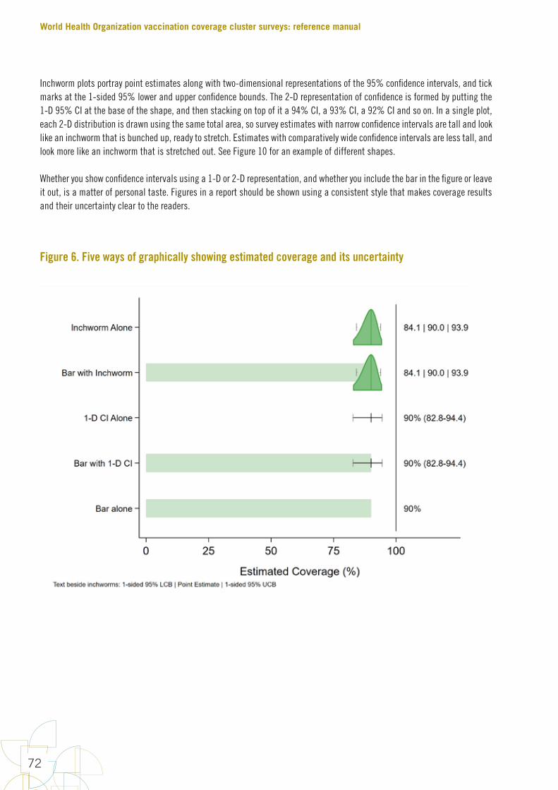
Inchworm plots portray point estimates along with two-dimensional representations of the 95% confidence intervals, and tick marks at the 1-sided 95% lower and upper confidence bounds. The 2-D representation of confidence is formed by putting the 1-D 95% CI at the base of the shape, and then stacking on top of it a 94% CI, a 93% CI, a 92% CI and so on. In a single plot, each 2-D distribution is drawn using the same total area, so survey estimates with narrow confidence intervals are tall and look like an inchworm that is bunched up, ready to stretch. Estimates with comparatively wide confidence intervals are less tall, and look more like an inchworm that is stretched out. See Figure 10 for an example of different shapes.
Whether you show confidence intervals using a 1-D or 2-D representation, and whether you include the bar in the figure or leave it out, is a matter of personal taste. Figures in a report should be shown using a consistent style that makes coverage results and their uncertainty clear to the readers.
Figure 6. Five ways of graphically showing estimated coverage and its uncertainty
World Health Organization vaccination coverage cluster surveys: reference manual
72
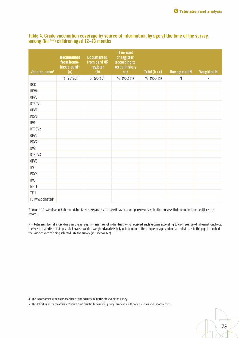
Table 4. Crude vaccination coverage by source of information, by age at the time of the survey, among (N=**) children aged 12–23 months
Vaccine, dose4
Documented from home-based card*
(a)
Documented, from card OR
register (b)
If no card or register,
according to verbal history
(c) Total (b+c) Unweighted N Weighted N % (95%CI) % (95%CI) % (95%CI) % (95%CI) N N
BCG
HBV0
OPV0
DTPCV1
OPV1
PCV1
RV1
DTPCV2
OPV2
PCV2
RV2
DTPCV3
OPV3
IPV
PCV3
RV3
MR 1
YF 1
Fully vaccinated5 45
* Column (a) is a subset of Column (b), but is listed separately to make it easier to compare results with other surveys that do not look for health centre records
N = total number of individuals in the survey. n = number of individuals who received each vaccine according to each source of information. Note: the % vaccinated is not simply n/N because we do a weighted analysis to take into account the sample design, and not all individuals in the population had the same chance of being selected into the survey (see section 6.2).
4 The list of vaccines and doses may need to be adjusted to fit the context of the survey.5 The definition of ‘fully vaccinated’ varies from country to country. Specify this clearly in the analysis plan and survey report.
6 Tabulation and analysis
73

Table 5. Crude and valid vaccination coverage
Vaccine, dose
Crude Coverage – documented evidence or caretaker recall of vaccination, (includes invalid doses and verbal history)Estimated % 95% CI 95% LCB 95% UCB
Valid Dose Coverage – documented evidence of vaccination at correct ages and with correct intervals (includes only valid doses)Estimated % 95% CI 95% LCB 95% UCB
BCG
HBV0
OPV0
DTPCV1
OPV1
PCV1
RV1
DTPCV2
OPV2
PCV2
RV2
DTPCV3
OPV3
IPV
PCV3
RV3 (if in schedule)
MR 1
YF
Fully vaccinated6 6
CI: confidence interval: LCB: lower confidence bound; UCB: upper confidence bound
(When N for the weighted valid coverage table is the same as N for the crude coverage table, it need not be repeated here.)
6 See earlier footnote on documenting the definition of ‘fully vaccinated’.
World Health Organization vaccination coverage cluster surveys: reference manual
74
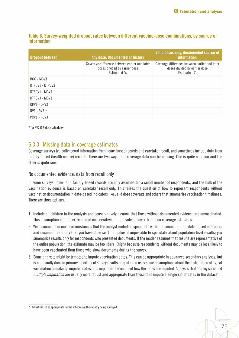
Table 6. Survey-weighted dropout rates between different vaccine-dose combinations, by source of information
Dropout between7 Any dose, documented or history Valid doses only, documented source of
informationCoverage difference between earlier and later
doses divided by earlier doseEstimated %
Coverage difference between earlier and later doses divided by earlier dose
Estimated %
BCG - MCV1
DTPCV1 - DTPCV3
DTPCV1 - MCV1
DTPCV3 - MCV1
OPV1 - OPV3
RV1 - RV3 *
PCV1 - PCV37
* (or RV2 if 2-dose schedule)
6.3.3. Missing data in coverage estimatesCoverage surveys typically record information from home-based records and caretaker recall, and sometimes include data from facility-based (health centre) records. There are two ways that coverage data can be missing. One is quite common and the other is quite rare.
No documented evidence; data from recall only
In some surveys home- and facility-based records are only availabe for a small number of respondents, and the bulk of the vaccination evidence is based on caretaker recall only. This raises the question of how to represent respondents without vaccination documentation in date-based indicators like valid dose coverage and others that summarize vaccination timeliness. There are three options:
1. Include all children in the analysis and conservatively assume that those without documented evidence are unvaccinated. This assumption is quite extreme and conservative, and provides a lower-bound on coverage estimates.
2. We recommend in most circumstances that the analyst exclude respondents without documents from date-based indicators and document carefully that you have done so. This makes it impossible to speculate about population level results; you summarize results only for respondents who presented documents. If the reader assumes that results are representative of the entire population, the estimate may be too liberal (high) because respondents without documents may be less likely to have been vaccinated than those who show documents during the survey.
3. Some analysts might be tempted to impute vaccination dates. This can be appropriate in advanced secondary analyses, but is not usually done in primary reporting of survey results. Imputation uses some assumptions about the distribution of age at vaccination to make up imputed dates. It is important to document how the dates are imputed. Analyses that employ so-called multiple imputation are usually more robust and appropriate than those that impute a single set of dates in the dataset.
7 Adjust the list as appropriate for the schedule in the country being surveyed.
6 Tabulation and analysis
75

Analysts should not simply assume that respondents without documents are vaccinated at the same ages as children who do present documented evidence. When estimating valid dose coverage or any other date-based indicator, some analysts may be tempted to suggest that children with cards are representative of those without cards. Unless the proportion of respondents with cards is very very high, that speculation is not appropriate for the primary results section of the report.
Traditionally, calculating valid coverage has conservatively considered respondents without documents are unvaccinated. The team writing the survey report will need to decide whether the audience is likely to understand this approach, in which some respondents in the denominator are not allowed into the numerator. In many cases, it will be more clear for the reader if respondents without documentation of vaccination are excluded from the calculation. The reader needs to be reminded that valid coverage may likely be lower among respondents without documentation of vaccination. Yet the survey data cannot tell us whether that is true or not.
Furthermore, traditionally, the percentage of children who receive a crude dose by age of 12 months has been calculated assuming, generously, that children without documents are vaccinated at the same ages as those with documents. In this manual, we recommend instead that respondents without documents be excluded from this calculation and that the report clearly states the proportion of respondents who were excluded from the calculation.
Regardless of what you decide, the survey report should be very clear about what proportion of respondents had documented vaccination history and how the respondents without documents were handled in date-based indicators.
No documented evidence and recall data is "Missing" or "Do Not Know"
Even in very well run surveys, a small number of eligible persons who lack vaccination documents might also be missing recall data due to an oversight, or might be coded to indicate that the caretaker “does not know (DNK)” whether their child received the dose. There are four possible approaches to handling missing or DNK recall data in coverage calculations:
1. Some analysts exclude these children from the calculation on a dose-by-dose basis; they are excluded from both the numerator and denominator of the coverage calculation. They are included if they have a non-missing response, but are not included if the response is missing or DNK. We do not recommend this approach. This child (and all the other children represented by this child’s survey weight) should be included in the coverage denominator of every dose using approach #3 or #4 below.
2. Some analysts might be tempted to impute responses to missing coverage data. For most situations we do not recommend this approach, either. The primary analysis should summarize the evidence collected during the survey. Speculation about unobserved evidence will involve various assumptions and could follow as a secondary analysis. But the primary analysis is typically not complicated in this manner.
3. Count any child with missing data or DNK as not vaccinated. This is a conservative approach, and the one we recommend. In most cases these children will represent a very small proportion of the total and may safely be grouped with those who were clearly not vaccinated.
4. Sometimes the missing/DNK category is large or conceptually important (maybe to emphasize the poor state of record-keeping in the country or to emphasize the very honest nature of the caretaker respondents). When this is the case, expand coverage summary tables to include three outcome categories:
» the % with evidence of vaccination
» the % with evidence that they are not vaccinated
» the % with missing data or DNK responses
(Tables may be expanded even further to itemize the sources of vaccination evidence: % with evidence from card, % with evidence from health centre, % with evidence from caretaker recall, etc.)
World Health Organization vaccination coverage cluster surveys: reference manual
76
6.4. Conduct additional analysesThis section describes additional analyses that can give very useful information to programme managers. Some rely on having a dataset with vaccination dates, thus, are restricted to children with documented vaccination and may be advisable only where availability of documented records is high.
Additional analysis options include:
• Missed opportunities analysis
• Vaccination by calendar month
• Assessment of the age at receipt of each dose (that is, validity and timeliness)
• Coverage by subgroups
• Comparing coverage between different locations in the same survey
• Comparing coverage over time
• Concordance across sources
• Co-administration or simultaneous vaccination for vaccines recommended at the same age
6.4.1. Missed opportunities8 In the context of a coverage survey, a missed opportunity for vaccination (MOV) is the failure to administer all vaccines for which the child was eligible (according to the national vaccination schedule) on the date of a clinic visit. For these analyses, only children having at least one documented date of vaccination are included. This analysis gives an idea of the prevalence of MOVs, but it is not possible to know by looking at a vaccination record whether the opportunity was truly missed or whether a real contraindication was present and the failure to vaccinate was a good decision.
For example, a child who received a first dose of DTPCV at age 6 weeks but did not receive pneumococcal conjugate vaccine (PCV) on the same date, when the national schedule recommended both at age 6 weeks and no true contraindication existed, has a MOV for PCV. A child may have multiple MOVs for a given vaccine. To read more about MOV, visit http://www.who.int/immunization/programmes_systems/policies_strategies/MOV/en/.
Two types of analyses are recommended: (1) visit-based analysis and (2) child-based analysis. As their names suggest, the visit-based analysis analyses the number of health facility visits of the children where there was 1+ MOV, whereas the child-based analysis analyses the number of children who experienced 1+ MOVs.
The steps to accomplish an MOV analysis are described briefly here, and in more detail in Annex O.
Visit-Based Analyses
The visit-based (VB) analysis consists of three calculations: the proportion of visits resulting in MOV for each vaccine (VB1), the proportion of visits resulting in at least one MOV across all vaccines (VB2), and the rate of MOVs per visit across all vaccines (VB3).
8 A high-quality analysis of missed opportunities depends very much on having a high-quality dataset of vaccination dates. Yet experience has shown that data entry clerks are more likely to make typographical errors when entering dates than when entering other types of data. It will be prudent to compare the dates on the photographs of home-based records and EPI registries with the dates in the dataset to evaluate the quality of the dataset. In order to ensure excellent data quality, it may be necessary to use photos of vaccination cards to confirm every date in the dataset.
6 Tabulation and analysis
77

(VB1) Proportion of visits resulting in an MOV for a given vaccine:
Numerator: Number of visits where a child received another vaccine (documented by card or register) and was eligible for the considered dose, but did not receive the considered dose
Denominator: Number of visits where a child was eligible to receive the considered dose
(VB2) Proportion of visits with at least one MOV (across all vaccines)
Numerator: Number of visits with at least one MOV (for any vaccine)
Denominator: Number of visits where a child was eligible to receive at least one vaccine
(VB3) Rate of MOVs per visit (across all vaccines)
Numerator: Number of MOVs summed across all vaccines (that is, sum of VB1 numerator across all vaccines)
Denominator: Number of visits where a child was eligible to receive at least one vaccine
Note: This calcuation is a rate, and so results greater than one are plausible.
Child-Based Analyses
The child-based (CB) analysis consists of two calculations: the proportion of children who had at least one MOV for a given vaccine (CB1), and the proportion of children with at least one MOV across all vaccines (CB2). CB1 can be further subdivided into the proportion of children who never received the particular vaccine (an uncorrected MOV), and those who did receive it by the time of the survey (a corrected MOV). Similarly, CB2 can be subdivided into the proportion of children where none, all, or some of the MOVs for the child were corrected by the time of the survey.
(CB1) Proportion of children who had at least one missed opportunity for a given vaccine:
Numerator: Number of children with at least one vaccination date recorded, who were eligible to receive the considered dose but did not receive the considered dose
Denominator: Number of children with at least one vaccination date recorded, who were eligible to receive the considered dose
Subdividing (CB1):
(CB1a) Proportion of children with uncorrected MOVs
Numerator: Children in (CB1) numerator who had not received the given vaccine by the time of the survey
Denominator: Same denominator as (CB1)
World Health Organization vaccination coverage cluster surveys: reference manual
78
(CB1b) Proportion of children with corrected MOVs
Numerator: Children in (CB1) numerator who had received the given vaccine at a later visit as documented by the vaccination card
Denominator: Same denominator as (CB1)
(CB2) Proportion of children who had at least one missed opportunity for any vaccine:
Numerator: Number of children with at least one vaccination date recorded who did not receive a vaccine/dose when they were eligible for it
Denominator: Number of children with at least one vaccination date recorded who were eligible to receive at least one vaccine/dose
Subdividing (CB2):
(CB2a) Proportion of children with no corrected MOVs
Numerator: Children in (CB2) numerator who had not received any of the missed vaccine(s) by the time of the survey
Denominator: Same denominator as (CB2)
(CB2b) Proportion of children with all corrected MOVs
Numerator: Children in (CB2) numerator who had received all the vaccine(s) at a later visit, as documented by the vaccination card or register
Denominator: Same denominator as (CB2)
(CB2c) Proportion of children with some corrected MOVs
Numerator: Children in (CB2) numerator who had received some, but not all, of the vaccine(s) at a later visit, as documented by the vaccination card or register
Denominator: Same denominator as (CB2)
After the visit-based and child-based MOV analyses are conducted, it is possible to calculate the potential coverage that could have been achieved if there had been no missed opportunities. This is done by re-estimating coverage while counting the children who had an uncorrected MOV for a given vaccine as if they had received the vaccine. This essentially moves these children from the “did not receive vaccine” group in the original coverage estimate calculation to the “documented from card” group. The coverage estimate is then recalculated, as shown in this table shell.
6 Tabulation and analysis
79
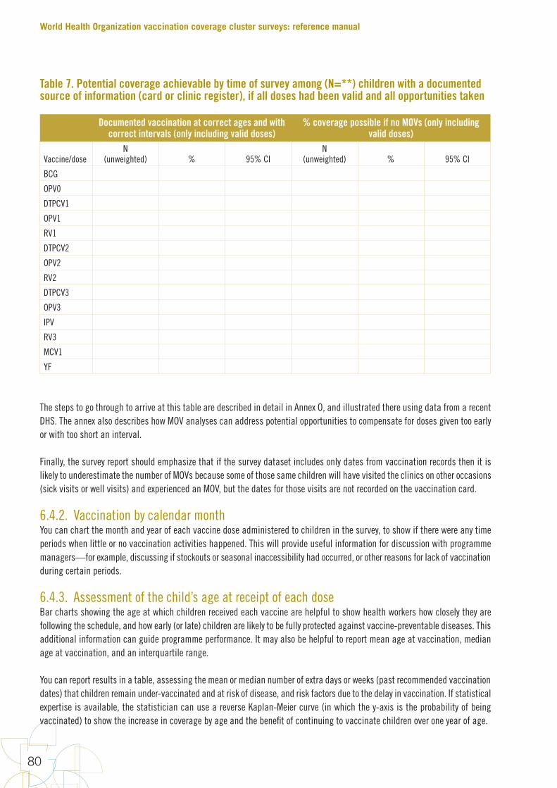
Table 7. Potential coverage achievable by time of survey among (N=**) children with a documented source of information (card or clinic register), if all doses had been valid and all opportunities taken
Documented vaccination at correct ages and with correct intervals (only including valid doses)
% coverage possible if no MOVs (only including valid doses)
Vaccine/doseN
(unweighted) % 95% CIN
(unweighted) % 95% CI
BCG
OPV0
DTPCV1
OPV1
RV1
DTPCV2
OPV2
RV2
DTPCV3
OPV3
IPV
RV3
MCV1
YF
The steps to go through to arrive at this table are described in detail in Annex O, and illustrated there using data from a recent DHS. The annex also describes how MOV analyses can address potential opportunities to compensate for doses given too early or with too short an interval.
Finally, the survey report should emphasize that if the survey dataset includes only dates from vaccination records then it is likely to underestimate the number of MOVs because some of those same children will have visited the clinics on other occasions (sick visits or well visits) and experienced an MOV, but the dates for those visits are not recorded on the vaccination card.
6.4.2. Vaccination by calendar monthYou can chart the month and year of each vaccine dose administered to children in the survey, to show if there were any time periods when little or no vaccination activities happened. This will provide useful information for discussion with programme managers—for example, discussing if stockouts or seasonal inaccessibility had occurred, or other reasons for lack of vaccination during certain periods.
6.4.3. Assessment of the child’s age at receipt of each dose Bar charts showing the age at which children received each vaccine are helpful to show health workers how closely they are following the schedule, and how early (or late) children are likely to be fully protected against vaccine-preventable diseases. This additional information can guide programme performance. It may also be helpful to report mean age at vaccination, median age at vaccination, and an interquartile range.
You can report results in a table, assessing the mean or median number of extra days or weeks (past recommended vaccination dates) that children remain under-vaccinated and at risk of disease, and risk factors due to the delay in vaccination. If statistical expertise is available, the statistician can use a reverse Kaplan-Meier curve (in which the y-axis is the probability of being vaccinated) to show the increase in coverage by age and the benefit of continuing to vaccinate children over one year of age.
World Health Organization vaccination coverage cluster surveys: reference manual
80
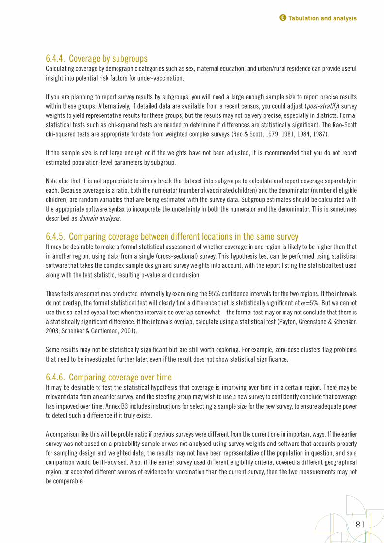
6.4.4. Coverage by subgroups Calculating coverage by demographic categories such as sex, maternal education, and urban/rural residence can provide useful insight into potential risk factors for under-vaccination.
If you are planning to report survey results by subgroups, you will need a large enough sample size to report precise results within these groups. Alternatively, if detailed data are available from a recent census, you could adjust (post-stratify) survey weights to yield representative results for these groups, but the results may not be very precise, especially in districts. Formal statistical tests such as chi-squared tests are needed to determine if differences are statistically significant. The Rao-Scott chi-squared tests are appropriate for data from weighted complex surveys (Rao & Scott, 1979, 1981, 1984, 1987).
If the sample size is not large enough or if the weights have not been adjusted, it is recommended that you do not report estimated population-level parameters by subgroup.
Note also that it is not appropriate to simply break the dataset into subgroups to calculate and report coverage separately in each. Because coverage is a ratio, both the numerator (number of vaccinated children) and the denominator (number of eligible children) are random variables that are being estimated with the survey data. Subgroup estimates should be calculated with the appropriate software syntax to incorporate the uncertainty in both the numerator and the denominator. This is sometimes described as domain analysis.
6.4.5. Comparing coverage between different locations in the same surveyIt may be desirable to make a formal statistical assessment of whether coverage in one region is likely to be higher than that in another region, using data from a single (cross-sectional) survey. This hypothesis test can be performed using statistical software that takes the complex sample design and survey weights into account, with the report listing the statistical test used along with the test statistic, resulting p-value and conclusion.
These tests are sometimes conducted informally by examining the 95% confidence intervals for the two regions. If the intervals do not overlap, the formal statistical test will clearly find a difference that is statistically significant at =5%. But we cannot use this so-called eyeball test when the intervals do overlap somewhat – the formal test may or may not conclude that there is a statistically significant difference. If the intervals overlap, calculate using a statistical test (Payton, Greenstone & Schenker, 2003; Schenker & Gentleman, 2001).
Some results may not be statistically significant but are still worth exploring. For example, zero-dose clusters flag problems that need to be investigated further later, even if the result does not show statistical significance.
6.4.6. Comparing coverage over timeIt may be desirable to test the statistical hypothesis that coverage is improving over time in a certain region. There may be relevant data from an earlier survey, and the steering group may wish to use a new survey to confidently conclude that coverage has improved over time. Annex B3 includes instructions for selecting a sample size for the new survey, to ensure adequate power to detect such a difference if it truly exists.
A comparison like this will be problematic if previous surveys were different from the current one in important ways. If the earlier survey was not based on a probability sample or was not analysed using survey weights and software that accounts properly for sampling design and weighted data, the results may not have been representative of the population in question, and so a comparison would be ill-advised. Also, if the earlier survey used different eligibility criteria, covered a different geographical region, or accepted different sources of evidence for vaccination than the current survey, then the two measurements may not be comparable.
6 Tabulation and analysis
81
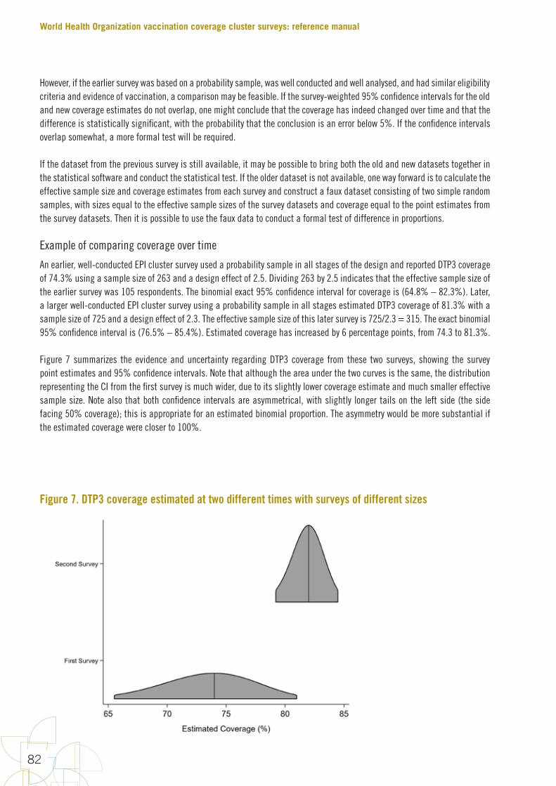
However, if the earlier survey was based on a probability sample, was well conducted and well analysed, and had similar eligibility criteria and evidence of vaccination, a comparison may be feasible. If the survey-weighted 95% confidence intervals for the old and new coverage estimates do not overlap, one might conclude that the coverage has indeed changed over time and that the difference is statistically significant, with the probability that the conclusion is an error below 5%. If the confidence intervals overlap somewhat, a more formal test will be required.
If the dataset from the previous survey is still available, it may be possible to bring both the old and new datasets together in the statistical software and conduct the statistical test. If the older dataset is not available, one way forward is to calculate the effective sample size and coverage estimates from each survey and construct a faux dataset consisting of two simple random samples, with sizes equal to the effective sample sizes of the survey datasets and coverage equal to the point estimates from the survey datasets. Then it is possible to use the faux data to conduct a formal test of difference in proportions.
Example of comparing coverage over time
An earlier, well-conducted EPI cluster survey used a probability sample in all stages of the design and reported DTP3 coverage of 74.3% using a sample size of 263 and a design effect of 2.5. Dividing 263 by 2.5 indicates that the effective sample size of the earlier survey was 105 respondents. The binomial exact 95% confidence interval for coverage is (64.8% – 82.3%). Later, a larger well-conducted EPI cluster survey using a probability sample in all stages estimated DTP3 coverage of 81.3% with a sample size of 725 and a design effect of 2.3. The effective sample size of this later survey is 725/2.3 = 315. The exact binomial 95% confidence interval is (76.5% – 85.4%). Estimated coverage has increased by 6 percentage points, from 74.3 to 81.3%.
Figure 7 summarizes the evidence and uncertainty regarding DTP3 coverage from these two surveys, showing the survey point estimates and 95% confidence intervals. Note that although the area under the two curves is the same, the distribution representing the CI from the first survey is much wider, due to its slightly lower coverage estimate and much smaller effective sample size. Note also that both confidence intervals are asymmetrical, with slightly longer tails on the left side (the side facing 50% coverage); this is appropriate for an estimated binomial proportion. The asymmetry would be more substantial if the estimated coverage were closer to 100%.
Figure 7. DTP3 coverage estimated at two different times with surveys of different sizes
World Health Organization vaccination coverage cluster surveys: reference manual
82
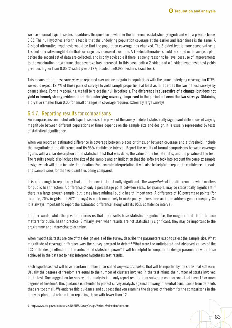
We use a formal hypothesis test to address the question of whether the difference is statistically significant with a p-value below 0.05. The null hypothesis for this test is that the underlying population coverage at the earlier and later times is the same. A 2-sided alternative hypothesis would be that the population coverage has changed. The 2-sided test is more conservative; a 1-sided alternative might state that coverage has increased over time. A 1-sided alternative should be stated in the analysis plan before the second set of data are collected, and is only advisable if there is strong reason to believe, because of improvements to the vaccination programme, that coverage has increased. In this case, both a 2-sided and a 1-sided hypothesis test yields p-values higher than 0.05 (2-sided p = 0.127; 1-sided p=0.083; Fisher’s Exact Test).
This means that if these surveys were repeated over and over again in populations with the same underlying coverage for DTP3, we would expect 12.7% of those pairs of surveys to yield sample proportions at least as far apart as the two in these surveys by chance alone. Formally speaking, we fail to reject the null hypothesis. The difference is suggestive of a change, but does not yield extremely strong evidence that the underlying coverage improved in the period between the two surveys. Obtaining a p-value smaller than 0.05 for small changes in coverage requires extremely large surveys.
6.4.7. Reporting results for comparisonsFor comparisons conducted with hypothesis tests, the power of the survey to detect statistically significant differences of varying magnitude between different populations or times depends on the sample size and design. It is usually represented by tests of statistical significance.
When you report an estimated difference in coverage between places or times, or between coverage and a threshold, include the magnitude of the difference and its 95% confidence interval. Report the results of formal comparisons between coverage figures with a clear description of the statistical test that was done, the value of the test statistic, and the p-value of the test. The results should also include the size of the sample and an indication that the software took into account the complex sample design, which will often include stratification. For accurate interpretation, it will also be helpful to report the confidence intervals and sample sizes for the two quantities being compared.
It is not enough to report only that a difference is statistically significant. The magnitude of the difference is what matters for public health action. A difference of only 1 percentage point between sexes, for example, may be statistically significant if there is a large enough sample, but it may have minimal public health importance. A difference of 10 percentage points (for example, 70% in girls and 80% in boys) is much more likely to make policymakers take action to address gender inequity. So it is always important to report the estimated difference, along with its 95% confidence interval.
In other words, while the p-value informs us that the results have statistical significance, the magnitude of the difference matters for public health practice. Similarly, even when results are not statistically significant, they may be important to the programme and interesting to examine.
When hypothesis tests are one of the design goals of the survey, describe the parameters used to select the sample size. What magnitude of coverage difference was the survey powered to detect? What were the anticipated and observed values of the ICC or the design effect, and the anticipated statistical power? It will be helpful to compare the design parameters with those achieved in the dataset to help interpret hypothesis test results.
Each hypothesis test will have a certain number of so-called degrees of freedom that will be reported by the statistical software. Usually the degrees of freedom are equal to the number of clusters involved in the test minus the number of strata involved in the test. One suggestion for survey data analysis is to only report results from subgroup comparisons that have 12 or more degrees of freedom9. This guidance is intended to protect survey analysts against drawing inferential conclusions from datasets that are too small. We endorse this guidance and suggest that you examine the degrees of freedom for the comparisons in the analysis plan, and refrain from reporting those with fewer than 12.
9 http://www.cdc.gov/nchs/tutorials/NHANES/SurveyDesign/VarianceEstimation/intro.htm
6 Tabulation and analysis
83
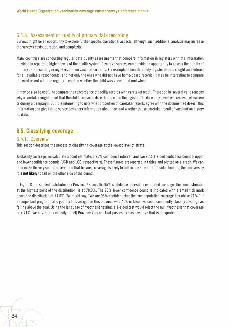
6.4.8. Assessment of quality of primary data recordingSurveys might be an opportunity to explore further specific operational aspects, although such additional analysis may increase the survey’s costs, duration, and complexity.
Many countries are conducting regular data quality assessments that compare information in registers with the information provided in reports to higher levels of the health system. Coverage surveys can provide an opportunity to assess the quality of primary data recording in registers and on vaccination cards. For example, if health facility register data is sought and entered for all available respondents, and not only the ones who did not have home-based records, it may be interesting to compare the card record with the register record on whether the child was vaccinated and when.
It may be also be useful to compare the concordance of facility records with caretaker recall. There can be several valid reasons why a caretaker might report that the child received a dose that is not in the register. The dose may have been received elsewhere or during a campaign. But it is interesting to note what proportion of caretaker reports agree with the documented doses. This information can give future survey designers information about how and whether to use caretaker recall of vaccination history as data.
6.5. Classifying coverage 6.5.1. OverviewThis section describes the process of classifying coverage at the lowest level of strata.
To classify coverage, we calculate a point estimate, a 95% confidence interval, and two 95% 1-sided confidence bounds: upper and lower confidence bounds (UCB and LCB, respectively). These figures are reported in tables and plotted on a graph. We can then make the very simple observation that because coverage is likely to fall on one side of the 1-sided bounds, then conversely it is not likely to fall on the other side of the bound.
In Figure 8, the shaded distribution for Province 7 shows the 95% confidence interval for estimated coverage. The point estimate, at the highest point of the distribution, is at 78.0%. The 95% lower confidence bound is indicated with a small tick mark above the distribution at 71.0%. We might say, “We are 95% confident that the true population coverage lies above 71%.” If an important programmatic goal for this antigen in this province was 71% or lower, we could confidently classify coverage as falling above the goal. Using the language of hypothesis testing, a 1-sided test would reject the null hypothesis that coverage is < 71%. We might thus classify (label) Province 7 as one that passes, or has coverage that is adequate.
World Health Organization vaccination coverage cluster surveys: reference manual
84
In Figure 9 the shaded 95% confidence interval is the same as in Figure 8, but now we indicate the upper 95% confidence bound with a tick mark at 83.7%. Note that the programmatic goal of 90% coverage is indicated with a blue vertical line. Although the confidence interval for Province 7 is quite wide (69.5% to 84.7%), we can confidently classify the coverage as being 95% likely to fall below 83.7%. So this province clearly fails to meet the goal of 90% coverage. When the programmatic goal lies above the 95% upper confidence bound, then we can confidently classify coverage as falling below the goal. Here, coverage fails, or is inadequate.
Figure 8. Point estimate, 95% confidence interval and 95% lower confidence bound for coverage in hypothetical province #7
Figure 9. Point estimate, 95% confidence interval and 95% upper confidence bound for coverage in hypothetical province #7
6 Tabulation and analysis
85
In the intermediate situation, where the programmatic goal falls between the upper and lower confidence bounds, we cannot classify coverage as above or below the threshold with 95% confidence. We would have needed to conduct a larger survey to do that. But looking at the graphic confidence intervals for all strata, especially if they are sorted in order of estimated coverage, will show where each stratum falls in the pattern and should provide actionable insight, especially regarding the strata with the lowest and highest levels of coverage.
It is not strictly necessary to portray what you learn from the survey graphically, but it is strongly recommended. You can present point estimates, confidence intervals, and upper and lower confidence bounds in a table only, but the results may not be clear to stakeholders who do not have a clear understanding of confidence intervals and limits. Portraying the two-dimensional distributions of estimated coverage, and showing them for all the strata in the survey at once, may be a powerful way to communicate what you have learned about coverage from the survey. It is also a powerful way of communicating what you have NOT learned, such as when true coverage is very near a programmatic threshold and the sample size is small. In this case, you cannot use the survey to confidently conclude whether that stratum is above or below the threshold of interest.
To sum up:
1. Classification and estimation use the same underlying processes: calculate a point estimate and a confidence interval, and portray them. When classifying, also portray the 1-sided confidence bounds and use those bounds (rather than the ends of the 2-sided confidence interval) to make strong statements about whether coverage is above or below an important threshold.
2. This can be done using only tables, but adding graphics may help some audiences understand what you have learned more easily than tables alone.
3. Rather than sort the strata in alphabetic or administrative order, it is helpful to sort them in order of estimated coverage, or in order of the upper or lower confidence bounds. See Figure 10 below.
4. This approach to classification may be used with either small or large sample sizes. As the sample size gets larger, the upper and lower confidence bounds will fall nearer and nearer to the coverage point estimate. Conversely, if the sample sizes are small, the confidence bounds will fall farther from the point estimate. However, the principle of using the bound to confidently characterize whether coverage is above or below a threshold of interest is the same, regardless of sample size.
5. It is permissible to both estimate and classify coverage using a single survey. When describing estimation results, we usually focus on saying that the coverage is likely to fall within a 2-sided confidence interval. When classifying, we focus on saying that coverage is likely to fall on one side of a confidence bound. We recommend using at least 15 clusters per stratum for classification and at least 30 clusters per stratum for precise estimation.
6.5.2. Examples of classificationTo classify coverage, calculate and plot the point estimate, the 95% CI, and the upper and lower 95% confidence bounds10. Recall that the 1-sided confidence bound is different than the endpoint of a 95% confidence interval. The 95% lower confidence bound can be calculated using the lower end of a 90% confidence interval. The 95% upper confidence bound can be calculated using the upper end of a 90% confidence interval. These bounds will fall inside the 95% confidence interval.
Figure 10 shows estimated measles SIA coverage for 24 fictional districts, based on samples of 15 clusters and 10 respondents per cluster in each district. For each district, the 95% confidence interval is indicated in light gray and the 95% upper and lower confidence bounds are indicated with small black tick marks. Three intervals are listed at the right side of each distribution. The first is the classic 2-sided 95% confidence interval. The second is the interval that extends from 0% coverage up to the 95% upper confidence bound. The third is the interval that extends from the 95% lower confidence bound up to coverage of 100%. All three intervals are equally valid for drawing conclusions with 95% confidence. The regions are plotted in increasing
10 Recall that we say informally that we are 95% confident that the true coverage falls within the 95% CI. We also say that we are 95% confident that true coverage falls somewhere above the 95% lower confidence bound, and we are 95% confident that the true coverage falls somewhere below the 95% upper confidence bound.
World Health Organization vaccination coverage cluster surveys: reference manual
86

order of coverage point estimate, from bottom to top. The red vertical line marks the spot where coverage is 95%, an important programmatic threshold for measles. The district data are aggregated to estimate province coverage (shaded with a light gray bar) very precisely.
Although all the districts had samples of the same size, the width of the confidence intervals varies substantially, reflecting district-level differences in sample coverage and in the underlying ICC. Many of the intervals are too wide for precise estimation, but the data in the figure can be used to classify coverage into two or more categories.
Any consistent categorization is permissible as long as it is useful and described clearly. The programmatic threshold of 95% coverage is important for measles campaigns. Several logical coverage categorizations are described in Annex N.
Figure 10. Measles SIA coverage and confidence interval and bounds for 24 fictional districts and the province that they comprise; districts are sorted by estimated coverage
Note: The distributions are plotted with equal areas, corresponding to 95% confidence for each district, so those with narrow confidence intervals appear taller and those with wider intervals have very little height. Tick marks near the left edge of each distribution indicate the 95% one-sided lower confidence bound; those near the right edge indicate the 95% one-sided upper confidence bound. The red vertical line indicates a programmatic threshold of 95% coverage. Districts coloured green are 95% likely to have coverage ≥ 95%. Those coloured red are 95% likely to have coverage < 95%. Those coloured yellow cannot be classified as above or below 95% with this sample of 150 respondents.
6 Tabulation and analysis
87


7Interpret, format, and share results
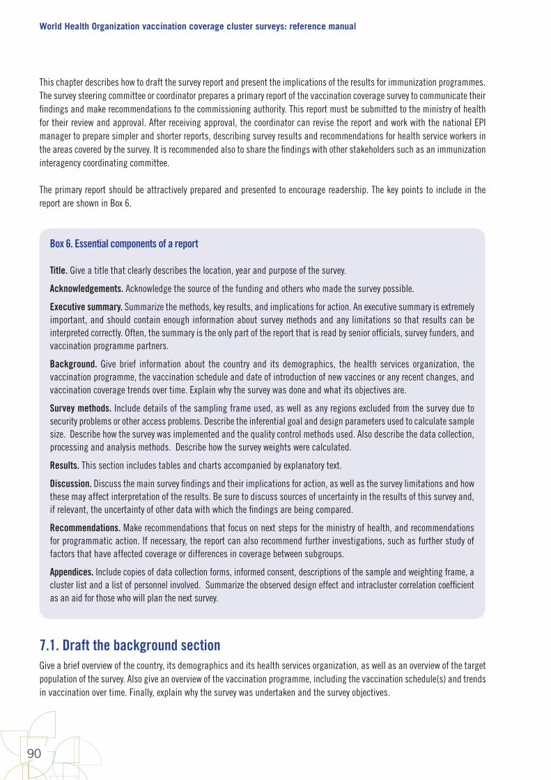
World Health Organization vaccination coverage cluster surveys: reference manual
90
This chapter describes how to draft the survey report and present the implications of the results for immunization programmes. The survey steering committee or coordinator prepares a primary report of the vaccination coverage survey to communicate their findings and make recommendations to the commissioning authority. This report must be submitted to the ministry of health for their review and approval. After receiving approval, the coordinator can revise the report and work with the national EPI manager to prepare simpler and shorter reports, describing survey results and recommendations for health service workers in the areas covered by the survey. It is recommended also to share the findings with other stakeholders such as an immunization interagency coordinating committee.
The primary report should be attractively prepared and presented to encourage readership. The key points to include in the report are shown in Box 6.
Box 6. Essential components of a report
Title. Give a title that clearly describes the location, year and purpose of the survey.
Acknowledgements. Acknowledge the source of the funding and others who made the survey possible.
Executive summary. Summarize the methods, key results, and implications for action. An executive summary is extremely important, and should contain enough information about survey methods and any limitations so that results can be interpreted correctly. Often, the summary is the only part of the report that is read by senior officials, survey funders, and vaccination programme partners.
Background. Give brief information about the country and its demographics, the health services organization, the vaccination programme, the vaccination schedule and date of introduction of new vaccines or any recent changes, and vaccination coverage trends over time. Explain why the survey was done and what its objectives are.
Survey methods. Include details of the sampling frame used, as well as any regions excluded from the survey due to security problems or other access problems. Describe the inferential goal and design parameters used to calculate sample size. Describe how the survey was implemented and the quality control methods used. Also describe the data collection, processing and analysis methods. Describe how the survey weights were calculated.
Results. This section includes tables and charts accompanied by explanatory text.
Discussion. Discuss the main survey findings and their implications for action, as well as the survey limitations and how these may affect interpretation of the results. Be sure to discuss sources of uncertainty in the results of this survey and, if relevant, the uncertainty of other data with which the findings are being compared.
Recommendations. Make recommendations that focus on next steps for the ministry of health, and recommendations for programmatic action. If necessary, the report can also recommend further investigations, such as further study of factors that have affected coverage or differences in coverage between subgroups.
Appendices. Include copies of data collection forms, informed consent, descriptions of the sample and weighting frame, a cluster list and a list of personnel involved. Summarize the observed design effect and intracluster correlation coefficient as an aid for those who will plan the next survey.
7.1. Draft the background sectionGive a brief overview of the country, its demographics and its health services organization, as well as an overview of the target population of the survey. Also give an overview of the vaccination programme, including the vaccination schedule(s) and trends in vaccination over time. Finally, explain why the survey was undertaken and the survey objectives.
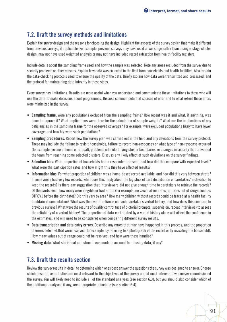
7 Interpret, format, and share results
91
7.2. Draft the survey methods and limitationsExplain the survey design and the reasons for choosing the design. Highlight the aspects of the survey design that make it different from previous surveys, if applicable. For example, previous surveys may have used a two-stage rather than a single-stage cluster design, may not have used weighted analysis or may not have included record extraction from health facility registers.
Include details about the sampling frame used and how the sample was selected. Note any areas excluded from the survey due to security problems or other reasons. Explain how data was collected in the field from households and health facilities. Also explain the data-checking protocols used to ensure the quality of the data. Briefly explain how data were transmitted and processed, and the protocol for maintaining data integrity in these steps.
Every survey has limitations. Results are more useful when you understand and communicate these limitations to those who will use the data to make decisions about programmes. Discuss common potential sources of error and to what extent these errors were minimized in the survey:
• Sampling frame. Were any populations excluded from the sampling frame? How recent was it and what, if anything, was done to improve it? What implications were there for the calculation of sample weights? What are the implications of any deficiencies in the sampling frame for the observed coverage? For example, were excluded populations likely to have lower coverage, and how big were such populations?
• Sampling procedures. Report how the survey plan was carried out in the field and any deviations from the survey protocol. These may include the failure to revisit households, failure to record non-responses or what type of non-response occurred (for example, no one at home or refusal), problems with identifying cluster boundaries, or changes in security that prevented the team from reaching some selected clusters. Discuss any likely effect of such deviations on the survey findings.
• Selection bias. What proportion of households had a respondent present, and how did this compare with expected levels? What were the participation rates and how might this they have affected results?
• Information bias. For what proportion of children was a home-based record available, and how did this vary between strata? If some areas had very few records, what does this imply about the logistics of card distribution or caretakers’ motivation to keep the records? Is there any suggestion that interviewers did not give enough time to caretakers to retrieve the records? Of the cards seen, how many were illegible or had errors (for example, no vaccination dates, or dates out of range such as DTPCV1 before the birthdate)? Did this vary by area? How many children without records could be traced at a health facility to obtain documentation? What was the overall reliance on each caretaker’s verbal history, and how does this compare to previous surveys? What were the results of quality control (use of pictorial prompts, supervision, repeat interviews) to assess the reliability of a verbal history? The proportion of data contributed by a verbal history alone will affect the confidence in the estimates, and will need to be considered when comparing different survey results.
• Data transcription and data entry errors. Describe any errors that may have happened in this process, and the proportion of errors detected that were resolved (for example, by referring to a photograph of the record or by revisiting the household). How many values out of range could not be resolved, and how were these handled?
• Missing data. What statistical adjustment was made to account for missing data, if any?
7.3. Draft the results sectionReview the survey results in detail to determine which ones best answer the questions the survey was designed to answer. Choose which descriptive statistics are most relevant to the objectives of the survey and of most interest to whomever commissioned the survey. You will likely need to include all of the standard analyses (see section 6.3), but you should also consider which of the additional analyses, if any, are appropriate to include (see section 6.4).

World Health Organization vaccination coverage cluster surveys: reference manual
92
Because survey results are based on a sample instead of a full census, they have some inherent uncertainty: if the survey were repeated using the same protocol and sample size, but a different set of households were visited, the results from those sampled households would vary somewhat from the ones sampled in this survey. This element of uncertainty, called sampling variability or sampling error, affects all survey results and is taken into account in different ways according to the type of result.
Select how you want to present the results, using the format that will make it easiest for the audience to understand the data. Diagrams and graphs are often most useful for communicating survey results. It is difficult to discern trends and draw conclusions from tables, but tables allow more detail to be presented. Tables should, therefore, be complemented by data visualizations. Decide which visualizations are most effective in drawing attention to the most important or relevant aspect of the data. Also consider visualizations that use color, lines and shapes to accurately portray the data. Choose visualizations that eliminate as much graphical clutter as possible.
In this manual we recommend the inchworm plot representation described in Chapter 6 for graphical display of coverage results. We recognize that bar charts are often used to portray coverage and are simpler to make than inchworm plots. If you portray coverage with a bar chart, be sure to include a representation of the 95% confidence interval on the chart to convey the magnitude of uncertainty due to sampling variability.
7.3.1. Describing results for estimates of coverageFor descriptive results such as estimates of coverage, the precision reflects sampling variability and is usually represented by the 95% confidence interval. The estimated proportion of eligible persons in the population who received each vaccine is called the point estimate of vaccination coverage. These estimates are often the main outcome of interest, and significant attention should be given to them.
7.3.2. Describing results for classifying coverageTo classify coverage, calculate the upper and lower 95% confidence bounds and compare those bounds to a pre-specified coverage threshold. It is always best to state classification rules clearly and report the upper and lower 95% confidence bounds to help readers gauge the strength of classification conclusions. Classify coverage as follows:
• When the lower 95% lower confidence bound falls above the threshold, confidently classify coverage as high; true coverage is very likely to be above the threshold.
• When the upper 95% confidence bound falls below the threshold, confidently classify coverage as low; true coverage is very likely to be below the threshold.
• When the threshold falls between the two bounds, conclude that the sample was not large enough at this level to classify with 95% confidence whether true coverage is above or below the threshold.
See Annex N for classification examples.
Some reports summarize classification results by simply listing which strata were classified as being high or low, but we discourage this practice. Reporting only the qualitative result may be helpful for simplicity, but it comes at the cost of omitting important information that may be useful to some readers of the report. Consider listing the confidence bounds for every classification result, so that readers of the report can compare coverage to other thresholds that may be of secondary interest. It is helpful to report and plot the 95% confidence interval along with the upper and lower confidence bounds for each coverage result, as shown in section 6.5.
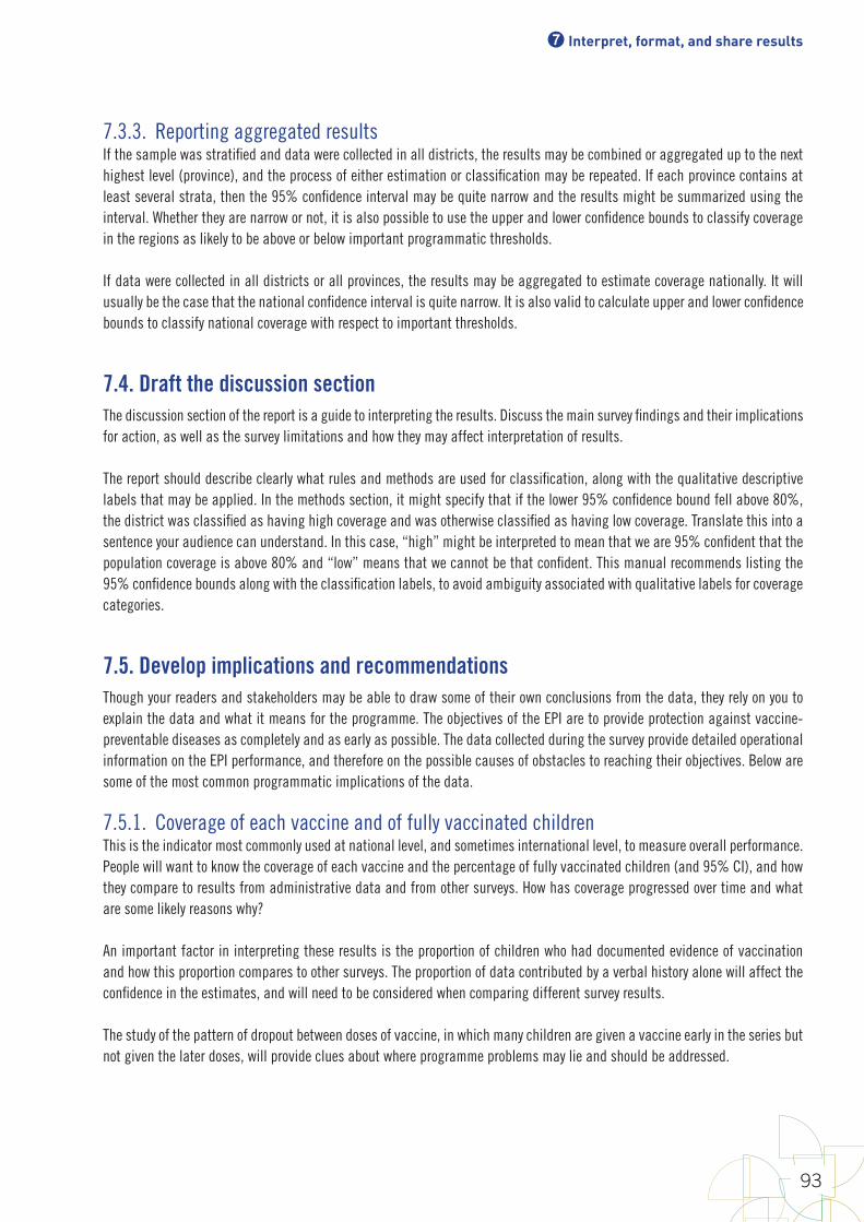
7 Interpret, format, and share results
93
7.3.3. Reporting aggregated resultsIf the sample was stratified and data were collected in all districts, the results may be combined or aggregated up to the next highest level (province), and the process of either estimation or classification may be repeated. If each province contains at least several strata, then the 95% confidence interval may be quite narrow and the results might be summarized using the interval. Whether they are narrow or not, it is also possible to use the upper and lower confidence bounds to classify coverage in the regions as likely to be above or below important programmatic thresholds.
If data were collected in all districts or all provinces, the results may be aggregated to estimate coverage nationally. It will usually be the case that the national confidence interval is quite narrow. It is also valid to calculate upper and lower confidence bounds to classify national coverage with respect to important thresholds.
7.4. Draft the discussion sectionThe discussion section of the report is a guide to interpreting the results. Discuss the main survey findings and their implications for action, as well as the survey limitations and how they may affect interpretation of results.
The report should describe clearly what rules and methods are used for classification, along with the qualitative descriptive labels that may be applied. In the methods section, it might specify that if the lower 95% confidence bound fell above 80%, the district was classified as having high coverage and was otherwise classified as having low coverage. Translate this into a sentence your audience can understand. In this case, “high” might be interpreted to mean that we are 95% confident that the population coverage is above 80% and “low” means that we cannot be that confident. This manual recommends listing the 95% confidence bounds along with the classification labels, to avoid ambiguity associated with qualitative labels for coverage categories.
7.5. Develop implications and recommendationsThough your readers and stakeholders may be able to draw some of their own conclusions from the data, they rely on you to explain the data and what it means for the programme. The objectives of the EPI are to provide protection against vaccine-preventable diseases as completely and as early as possible. The data collected during the survey provide detailed operational information on the EPI performance, and therefore on the possible causes of obstacles to reaching their objectives. Below are some of the most common programmatic implications of the data.
7.5.1. Coverage of each vaccine and of fully vaccinated childrenThis is the indicator most commonly used at national level, and sometimes international level, to measure overall performance. People will want to know the coverage of each vaccine and the percentage of fully vaccinated children (and 95% CI), and how they compare to results from administrative data and from other surveys. How has coverage progressed over time and what are some likely reasons why?
An important factor in interpreting these results is the proportion of children who had documented evidence of vaccination and how this proportion compares to other surveys. The proportion of data contributed by a verbal history alone will affect the confidence in the estimates, and will need to be considered when comparing different survey results.
The study of the pattern of dropout between doses of vaccine, in which many children are given a vaccine early in the series but not given the later doses, will provide clues about where programme problems may lie and should be addressed.

World Health Organization vaccination coverage cluster surveys: reference manual
94
7.5.2. Reaching a birth cohortSometimes the results indicate that there was difficulty in reaching a certain birth cohort. • DPTCV1/BCG crude coverage by record, history, and register is an indicator of access to vaccination services (the percentage
reached at least once as well as the percentage of children who have never received these vaccines). Access should be quite high in most settings nowadays. It is worth looking carefully at the clusters where none of the children in the survey received DPTCV1/BCG. Which health facilities serve those clusters, and how is it possible that so many children in the sample were not vaccinated?
• Dropouts between the first vaccine and the last vaccine to be provided (for DTPCV1 and MCV1) may be an indicator of the EPI’s capacity of the EPI to follow-up with each birth cohort (and of utilization). What was the dropout between first and final doses of multi-dose vaccines? What were the likely reasons? Have dropout rates fallen since the last survey? If dropout rates are still high (for example, above 10 %), what strategies are needed to ensure that all children who start the vaccination series complete it? The data can provide clues about where programme problems may lie. Infant death rates and migrations influence the dropout rate, but so does the dissatisfaction of the families with the programme (irregular vaccination sessions, lack of information, fever or abscess following vaccination, etc.).
7.5.3. Quality of recording and reporting vaccinationsSometimes the data suggest that the issue is not necessarily with administration of the vaccine, but with reporting when vaccines were administered and to whom. Questions to consider: • Is there an important difference between survey coverage results and administrative reports, and does this vary by stratum?
The data may help indicate potential problems with the numerators, denominators or both used in administrative estimates.
• What proportion of individuals in the survey had a home-based record available, and has this improved since previous surveys? What proportion said that they had received one but did not have it available at the time of the survey? What are the likely reasons for lack of cards (such as stockouts, failure to emphasize their importance, caretakers not keeping them after the vaccination series has been completed)?
• How well were vaccination records completed? What proportion of records had dates that were outside the valid range (for example, date of birth after date of DTPCV1)? What proportion had illegible or missing dates (for example, tick marks instead of dates)?
• What proportion of children’s vaccination records was located in health facility records? For those not located, what were the likely reasons (for example, migrants, poor storage of health facility records, stockouts)?
• What was the quality of health facility records? How many illegible entries or out-of-range entries were found?
• Depending on survey design, health facility records may have been sought for all children, or only for children who did not have a home-based record. If sought for all children, how did data from health facility records compare with those from home-based records, and what are some likely reasons for discrepancies?
• Are dropout rates in the survey similar to those reported from administrative data? If routine reports show much lower dropout rates than survey results, investigate how well health workers are recording each dose of vaccine. Sometimes they may intentionally record the first or second dose of DTPCV1 incorrectly as the third dose, because they know that the third dose is monitored more closely.
7.5.4. Invalid doses and timely encounters Many problems with low vaccination rates can be corrected by better adherence to the vaccination schedules and standards.
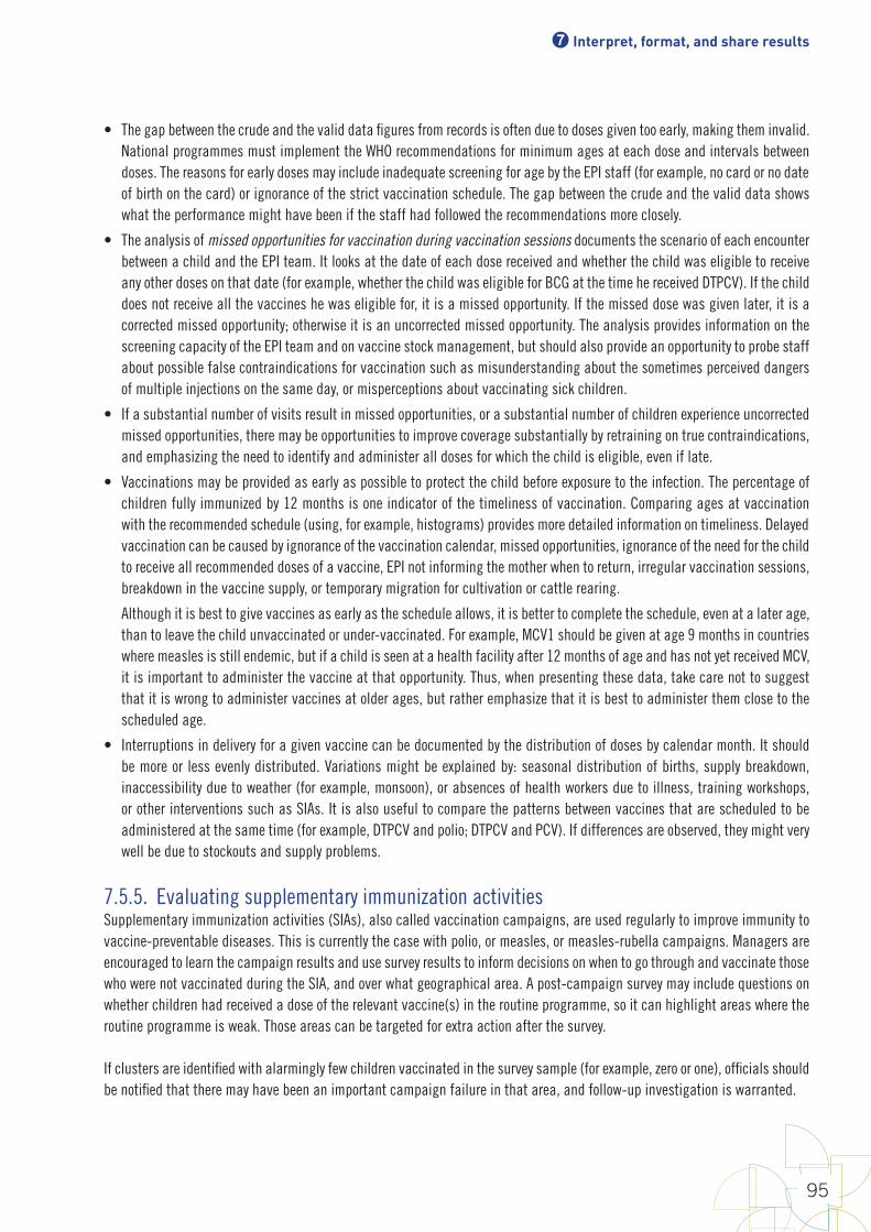
7 Interpret, format, and share results
95
• The gap between the crude and the valid data figures from records is often due to doses given too early, making them invalid. National programmes must implement the WHO recommendations for minimum ages at each dose and intervals between doses. The reasons for early doses may include inadequate screening for age by the EPI staff (for example, no card or no date of birth on the card) or ignorance of the strict vaccination schedule. The gap between the crude and the valid data shows what the performance might have been if the staff had followed the recommendations more closely.
• The analysis of missed opportunities for vaccination during vaccination sessions documents the scenario of each encounter between a child and the EPI team. It looks at the date of each dose received and whether the child was eligible to receive any other doses on that date (for example, whether the child was eligible for BCG at the time he received DTPCV). If the child does not receive all the vaccines he was eligible for, it is a missed opportunity. If the missed dose was given later, it is a corrected missed opportunity; otherwise it is an uncorrected missed opportunity. The analysis provides information on the screening capacity of the EPI team and on vaccine stock management, but should also provide an opportunity to probe staff about possible false contraindications for vaccination such as misunderstanding about the sometimes perceived dangers of multiple injections on the same day, or misperceptions about vaccinating sick children.
• If a substantial number of visits result in missed opportunities, or a substantial number of children experience uncorrected missed opportunities, there may be opportunities to improve coverage substantially by retraining on true contraindications, and emphasizing the need to identify and administer all doses for which the child is eligible, even if late.
• Vaccinations may be provided as early as possible to protect the child before exposure to the infection. The percentage of children fully immunized by 12 months is one indicator of the timeliness of vaccination. Comparing ages at vaccination with the recommended schedule (using, for example, histograms) provides more detailed information on timeliness. Delayed vaccination can be caused by ignorance of the vaccination calendar, missed opportunities, ignorance of the need for the child to receive all recommended doses of a vaccine, EPI not informing the mother when to return, irregular vaccination sessions, breakdown in the vaccine supply, or temporary migration for cultivation or cattle rearing.
Although it is best to give vaccines as early as the schedule allows, it is better to complete the schedule, even at a later age, than to leave the child unvaccinated or under-vaccinated. For example, MCV1 should be given at age 9 months in countries where measles is still endemic, but if a child is seen at a health facility after 12 months of age and has not yet received MCV, it is important to administer the vaccine at that opportunity. Thus, when presenting these data, take care not to suggest that it is wrong to administer vaccines at older ages, but rather emphasize that it is best to administer them close to the scheduled age.
• Interruptions in delivery for a given vaccine can be documented by the distribution of doses by calendar month. It should be more or less evenly distributed. Variations might be explained by: seasonal distribution of births, supply breakdown, inaccessibility due to weather (for example, monsoon), or absences of health workers due to illness, training workshops, or other interventions such as SIAs. It is also useful to compare the patterns between vaccines that are scheduled to be administered at the same time (for example, DTPCV and polio; DTPCV and PCV). If differences are observed, they might very well be due to stockouts and supply problems.
7.5.5. Evaluating supplementary immunization activitiesSupplementary immunization activities (SIAs), also called vaccination campaigns, are used regularly to improve immunity to vaccine-preventable diseases. This is currently the case with polio, or measles, or measles-rubella campaigns. Managers are encouraged to learn the campaign results and use survey results to inform decisions on when to go through and vaccinate those who were not vaccinated during the SIA, and over what geographical area. A post-campaign survey may include questions on whether children had received a dose of the relevant vaccine(s) in the routine programme, so it can highlight areas where the routine programme is weak. Those areas can be targeted for extra action after the survey.
If clusters are identified with alarmingly few children vaccinated in the survey sample (for example, zero or one), officials should be notified that there may have been an important campaign failure in that area, and follow-up investigation is warranted.
World Health Organization vaccination coverage cluster surveys: reference manual
96
7.6. Revise the report and obtain clearance on final draftA draft report should be prepared as soon as possible after the survey ends, and presented to national authorities (and, if possible, to health authorities in each stratum of the survey). Often, when presenting results, additional issues will be raised that will lead to fuller discussion of the results and their implications. The report should be updated accordingly, and the final report submitted to all relevant institutions. It will be necessary to obtain clearance on the final report from the ministry of health before distributing it widely.
7.7. Share the resultsAlthough the coverage survey results might initially seem to be a technical subject only, in practice they can become political and sensitive, and should be approached as such. The survey organizers should be aware that survey results should sometimes be perceived as an assessment of the performance of the specific programmes implementing the SIA, and indirectly of the institutions (EPI, ministry of health), and potentially of the government and the political parties in power.
The survey is not simply an academic exercise or a formal requirement for international donor and technical agencies. Rather, it produces data that could be used to improve the EPI at each level. Therefore, it is essential that each level of stakeholders understands the implications of the results, and how they can facilitate corrective actions. Because of this, it is important to think through how you will share the results. Below are some steps to consider taking as you plan to share the survey results.
7.7.1. Choose the key messagesThere are usually a few main themes that emerge from the data. Create messages based on these themes. Consider the survey goals and the political context as you create messages.
Phrase the conclusions and the recommendations of the report in objective, moderate terms, stating the facts and their meaning. The general tone should be not to blame but to emphasize progress, while documenting the possible reasons for slow progress and opportunities for improvement. The recommendations should stem practically from an interpretation of the results that would have been expressed in operational terms. For example, a DTPCV first dose coverage of 87% will be interpreted as 13% of children not being reached, and the recommendation will be to document the profile of these children in order to reach them in the future.
Ideally, the following will be true when it is time to share the results:
• The organization of the survey (including the selection of a contractor) has been requested and approved by the Ministry of Health at the beginning of the process.
• The reliability of the data collection and of the data processing have been checked and documented thoroughly.
• The interpretation of the data has been peer reviewed at least by the following: the steering group, the survey coordinator, the statistician, the EPI director, and senior members of the ministry of health.
If any of these has not been done, you will need additional talking points to address what happened and why.

7 Interpret, format, and share results
97
7.7.2. Select audiences Consider who needs to learn about the survey results and how best to communicate them. Priority should be given to the policymakers, but also to the local EPI managers who will take corrective action. The goal of the survey is to provide actionable information to the EPI managers at different levels to take corrective action. It is essential that the presentation of the results and their implications go beyond a national presentation to multiple administrative levels (provinces, districts, etc.). The level that can make the most impactful changes based on survey results is probably the lowest statistically valid stand-alone level, the strata at the lowest level of administrative hierarchy.
It is also important to give feedback to all relevant partners (which could be done in a meeting of the interagency coordinating committee), including health facility workers, other providers in the area and senior health officials. Feedback should be ideally provided soon, ideally within one month, and is most effective if provided through meetings or newsletters. Feedback helps make health facility staff feel that they are an important part of the vaccination services, thereby increasing their motivation. Communities covered by the survey should also receive feedback, presented in ways appropriate to a lay audience.
The survey budget should include the costs of workshops designed for the EPI manager or deputies and the local EPI staff. During these sessions, attendees will discuss the probable causes of any weaknesses or incomplete performance, and identify corrective actions along with their costs and timetables.
If there are topics for which the team does not have enough information, the EPI should do focused operational research. For example, they could look into health facility studies of missed opportunities and their causes, or conduct focus groups to assess community attitudes and knowledge. In any case, once completed, a survey is likely to translate in to strategies for improvements, and such strategies cost money. At the time of evaluating the survey and its financial feasibility, also investigate the availability of funds to implement its recommendations.
7.7.3. Create communication pieces and presentationsPrepare other forms of communication in addition to the survey report. The purpose of the survey, ultimately, is to improve vaccination practices and vaccination rates, so it is essential to communicate with district health offices so they can learn from the survey results and improve practices.
Use slide presentations for feedback workshops, and create a brief summary of the national survey results, as well as province- or district-specific results and recommendations, for all districts. You can also print four or five of the key charts and tables (for example, coverage by the time of the survey, by stratum, histogram of age at DTPCV1 and MCV1, and tables summarizing crude and valid coverage and missed opportunities), with bullet points showing their implications for action. These can be used for widespread distribution to health workers.
The high officials attending the presentation meeting should be provided the report or an executive summary in advance, to give them an opportunity to voice any questions and receive satisfactory answers before the beginning of the meeting.
7.7.4. Contribute micro-data, documentation, and code to a Coverage Survey RepositorySurvey data (stripped of names) and documentation of survey methods will be of greatest use if they are made freely available via the Internet, as is done for DHS and MICS. WHO is setting up a coverage survey repository that can be used to share vaccination coverage survey data. Details of survey methods (including the programs used to analyse the data) should accompany the micro-data of the survey. See the American Association for Public Opinion Research Transparency Initiative1 for more information on this issue.
1 http://www.aapor.org/Standards-Ethics/Transparency-Initiative/FAQs.aspx
World Health Organization vaccination coverage cluster surveys: reference manual
20
References
Brogan D, Flagg EW, Deming M, Waldman R (1994). Increasing the accuracy of the Expanded Programme on Immunization's cluster survey design. Annals of Epidemiology. 4(4):302–311.
Brown LD, Cai TT, DasGupta A (2001). Interval estimation for a binomial proportion. Stat Sci. 16:101–133.
Chipchase, Jan (2017). The Field Study Handbook. San Francisco: Field Institute.
Cochran, WG (1977). Sampling techniques, third edition. New York: John Wiley and Sons, Inc.
Cutts FT, Izurieta H, Rhoda DA (2013). Measuring coverage in MNCH: design, implementation and interpretation challenges associated with tracking vaccination coverage using household surveys. PLoS Med. 10(5).
Cutts, F. T., Claquin, P., Danovaro-Holliday, M. C., & Rhoda, D. A. (2016). Monitoring vaccination coverage: defining the role of surveys. Vaccine. 34(35):4103-4109.
Cutts, F.T & Hanson M. (2016). Seroepidemiology: an underused tool for designing and monitoring vaccination programmes in low- and middle-income countries. Trop Med and Intern Health. 21(9):1086-1098.
Dayan, GH, Shaw, KM, Baughman, AL, Orellana, LC, Forlenza, R, Ellis, A, Chaui, J, Kaplan S, & Strebel, P. (2006). Assessment of delay in age-appropriate vaccination using survival analysis. Am J Epidemiol. 163.6:561–570.
Driscoll J, Lidow, N (2014). Representative surveys in insecure environments: a case study of Mogadishu, Somalia. J Surv Stat and Methodol. 2:78–95.
Fleiss JL, Levin B, Paik MC (2003). Statistical methods for rates and proportions. Hoboken, NJ, USA: John Wiley & Sons, Inc.
Grais, R. F., Rose, A. M., & Guthmann, J. P. (2007). Don’t spin the pen: two alternative methods for second-stage sampling in urban cluster surveys. Emerg Themes Epidemiol, 4(8):1-7.
Hancioglu A, Arnold F (2013). Measuring coverage in MNCH: tracking progress in health for women and children using DHS and MICS household surveys. PLoS Med. 10(5).
Heeringa SG, West BT, Berglund PA (2010). Applied survey data analysis. Boca Raton, FL, USA: CRC Press.
Henderson RH, Sundaresan T (1982). Cluster sampling to assess immunization coverage: a review of experience with a simplified sampling method. Bull World Health Organ. 60(2):253.
Hutchins SS, Jansen HA, Robertson SE, Evans P, Kim-Farley, RJ (1993). Studies of missed opportunities for immunization in developing and industrialized countries. Bull World Health Organ. 71(5):549.
ICF International (2012a). Demographic and Health Survey sampling and household listing manual. MEASURE DHS. Calverton, MD, USA: ICF International.
ICF International (2012b). Survey organization manual for demographic and health surveys. MEASURE DHS. Calverton, MD, USA: ICF International.
Kalton, Graham, J. Michael Brick, and Thanh Lê. Estimating components of design effects for use in sample design. Household Sample Surveys in Developing and Transition Countries (2005): 95-121. https://unstats.un.org/unsd/hhsurveys/

References
99
Kish, L. (1987). Weighting in Deft. The Survey Statistician. The Newsletter of the International Association of Survey Statisticians, June.
Kish, Leslie (1965). Survey sampling. New York: John Wiley and Sons, Inc.
Korn EL, Graubard BI (1998). Confidence intervals for proportions with small expected number of positive counts estimated from survey data. Surv Methodol. 24:193–201.
Levy PS, Lemeshow S (1980). Sampling for health professionals, vol. 14. Belmont, CA, USA: Lifetime Learning Publications.
Levy PS, Lemeshow, S. (2013). Sampling of populations: methods and applications. Hoboken, NJ, USA: John Wiley & Sons, Inc.
Lohr, Sharon (2009). Sampling: design and analysis, second edition. Boston, MA, USA: Cengage Learning.
MacNeil, A., Lee, C. W., & Dietz, V. (2014). Issues and considerations in the use of serologic biomarkers for classifying vaccination history in household surveys. Vaccine. 32(39):4893-4900.
Meyer SA, Kambou JL, Cohn A, Goodson JL, Flannery B, Medah I, Messonnier N, Novak R, Diomande F, Djingarey MH, Clark TA, Yameogo I, Fall A, & Wannemuehler K. (2015). Serogroup A meningococcal conjugate (PsA-TT) vaccine coverage and measles vaccine coverage in Burkina Faso—implications for introduction of PsA-TT into the Expanded Programme on Immunization. Vaccine. 33(12):1492–8.
Park, Inho, Marianne Winglee, Jay Clark, Keith Rust, Andrea Sedlak, and David Morganstein. Design effects and survey planning. Joint Statistical Meetings – Section on Survey Research Methods (2003). http://ww2.amstat.org/sections/srms/proceedings/y2003/Files/JSM2003-000820.pdf
Payton ME, Greenstone MH, Schenker N (2003). Overlapping confidence intervals or standard error intervals: what do they mean in terms of statistical significance? J of Insect Science 3.1:34.
Rao JNK, Scott, AJ (1979). Chi-squared tests for analysis of categorical data from complex surveys. Proceedings of the Survey Research Methods Section, ASA. 58–66.
Rao JNK, Scott AJ (1981). The analysis of categorical data from complex surveys: chi-squared tests for goodness of fit and independence in two-way tables. J of the Am Stat Assn. 76:221–230.
Rao JNK, Scott, AJ (1984). On chi-squared tests for multiway contingency tables with cell properties estimated from survey data. Ann of Statistics. 12:46–60.
Rao JNK, and Scott AJ (1987). On simple adjustments to chi-square tests with survey data. Ann of Statistics. 15:385–397.
Schenker N, Gentleman JF (2001). On judging the significance of differences by examining the overlap between confidence intervals. Am Stat. 55.3:182–186.
Sridhar S, Maleq N, Guillermet E, Colombini A, Gessner BD (2014). A systematic literature review of missed opportunities for immunization in low- and middle-income countries. Vaccine. 32(51):6870–6879.
Valliant R, Dever JA, Kreuter F (2013). Practical tools for designing and weighting survey samples. New York: Springer.
World Health Organization (2005). Immunization coverage cluster survey: reference manual. WHO/IVB/04.23
World Health Organization (2011). Documenting the impact of Hepatitis B immunization: best practices for conducting a serosurvey. (http://whqlibdoc.who.int/hq/2011/WHO_IVB_11.08_eng.pdf?ua=1; accessed March 6, 2015)
Vaccination Coverage Quality Indicators (VCQI) references and materials may be found on the WHO vaccination coverage survey webpage: http://www.who.int/immunization/monitoring_surveillance/routine/coverage/en/, under survey methods

World Health Organization vaccination coverage cluster surveys: reference manual
100
ANNEXES
Annex A: Glossary of terms1-sided test A statistical test when the difference tested is directionally specified beforehand; for example, testing
whether vaccination coverage is higher in one area than in another. For vaccination coverage, in the language of statistical hypothesis tests, the null hypothesis (H0) for a 1-sided test is that coverage is on one side of a threshold and the alternative hypothesis is that coverage is on the other side of that threshold. For example, H0: coverage for DTPCV3 < 80% and the alternative hypothesis (HA): coverage ≥80%. Likewise, the null hypothesis could be that coverage in stratum A is equal to that in stratum B, and the alternative hypothesis could be that coverage in A is greater than coverage in B.
2-sided test A statistical test when the difference tested is not directionally specified beforehand; for example, testing whether vaccination coverage equals a specific value. In the language of hypothesis testing, the null hypothesis for a 2-sided test is that coverage is equal to a specific value, and the alternative hypothesis is that it is not equal to (either below or above) that value. Likewise, the null hypothesis could be that coverage in stratum A is equal to that in stratum B, and the alternative would be that coverage is not equal, but the alternative would not specify which of the two is higher.
Alpha () In parameter estimation, alpha is the probability value used to define the precision for estimated confidence intervals. Alpha is typically set to 0.05 and the corresponding confidence intervals are 95% confidence intervals, where 95% = 100 x (1 – )%.
In hypothesis testing, alpha is the probability of making a Type I error: rejecting the null hypothesis when in fact the null hypothesis is true.
Beta () In hypothesis testing, beta is the probability of making a Type II error: failing to reject the null hypothesis when in fact the null is false.
Bias Tendency of a sample statistic to systematically over- or under-estimate a population parameter
Classification (of coverage) A quantitative process of assigning a descriptive label to the estimated level of vaccination coverage. Labels might include high, low, adequate, inadequate, above the threshold, below the threshold or indeterminate.
Classification rules that use a single coverage threshold to divide results into two categories often provide one strong conclusion and one weak conclusion. This manual recommends using three classification outcomes: likely to be higher than the threshold, likely to be lower than the threshold, and indeterminate due to limited sample size.
Cluster A collection of elements (for example, households, communities, villages, census enumeration areas, etc.) grouped within defined geographical or administrative boundaries.
Cluster survey A survey in which the population under study is divided into an exhaustive and mutually exclusive set of primary sampling units (clusters), and a subset of those clusters is randomly selected for sampling.
Confidence bounds In this manual, confidence bounds mean 1-sided confidence limits. The upper confidence bound (UCB) is the upper limit of the 100 x (1 – )% confidence interval whose lower limit is 0%; the lower confidence bound (LCB) is the lower end of the 100 x (1 – )% confidence interval whose upper limit is 100%. Alpha is usually set to 0.05, so we say that we are 95% confident that the population parameter falls above the LCB, or we say that we are 95% confident that it falls below the UCB.
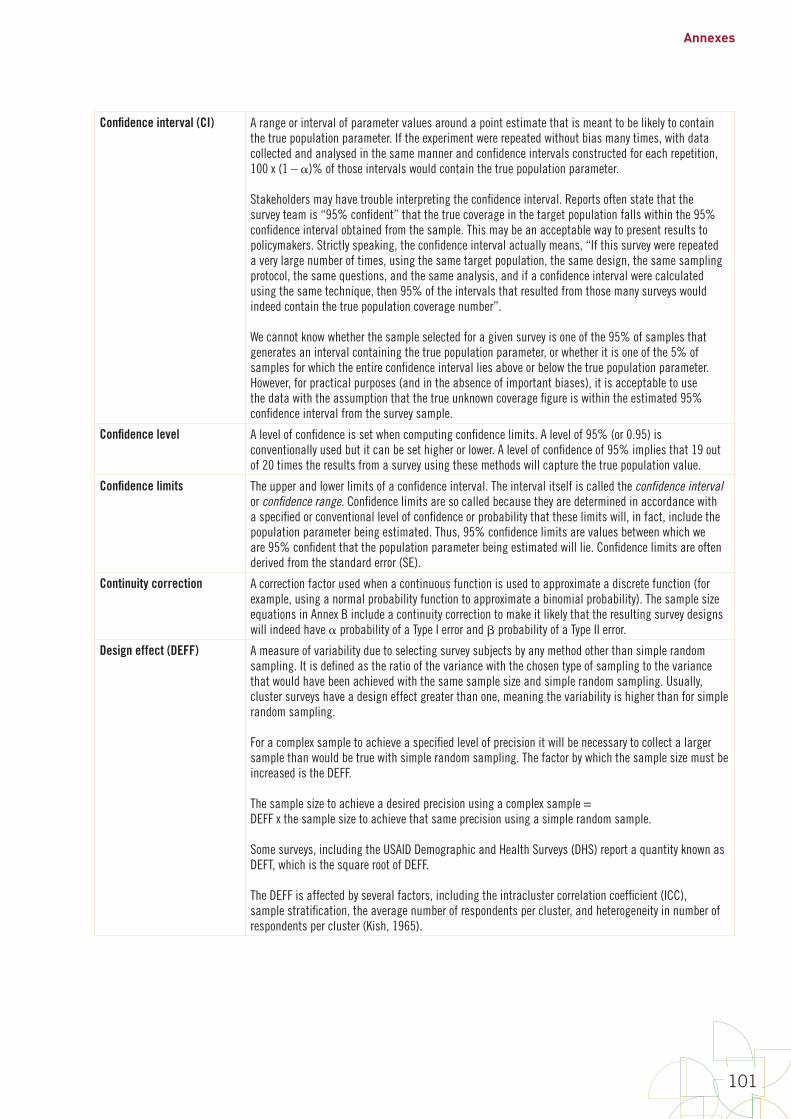
Annexes
101
Confidence interval (CI) A range or interval of parameter values around a point estimate that is meant to be likely to contain the true population parameter. If the experiment were repeated without bias many times, with data collected and analysed in the same manner and confidence intervals constructed for each repetition, 100 x (1 – )% of those intervals would contain the true population parameter.
Stakeholders may have trouble interpreting the confidence interval. Reports often state that the survey team is “95% confident” that the true coverage in the target population falls within the 95% confidence interval obtained from the sample. This may be an acceptable way to present results to policymakers. Strictly speaking, the confidence interval actually means, “If this survey were repeated a very large number of times, using the same target population, the same design, the same sampling protocol, the same questions, and the same analysis, and if a confidence interval were calculated using the same technique, then 95% of the intervals that resulted from those many surveys would indeed contain the true population coverage number”. We cannot know whether the sample selected for a given survey is one of the 95% of samples that generates an interval containing the true population parameter, or whether it is one of the 5% of samples for which the entire confidence interval lies above or below the true population parameter. However, for practical purposes (and in the absence of important biases), it is acceptable to use the data with the assumption that the true unknown coverage figure is within the estimated 95% confidence interval from the survey sample.
Confidence level A level of confidence is set when computing confidence limits. A level of 95% (or 0.95) is conventionally used but it can be set higher or lower. A level of confidence of 95% implies that 19 out of 20 times the results from a survey using these methods will capture the true population value.
Confidence limits The upper and lower limits of a confidence interval. The interval itself is called the confidence interval or confidence range. Confidence limits are so called because they are determined in accordance with a specified or conventional level of confidence or probability that these limits will, in fact, include the population parameter being estimated. Thus, 95% confidence limits are values between which we are 95% confident that the population parameter being estimated will lie. Confidence limits are often derived from the standard error (SE).
Continuity correction A correction factor used when a continuous function is used to approximate a discrete function (for example, using a normal probability function to approximate a binomial probability). The sample size equations in Annex B include a continuity correction to make it likely that the resulting survey designs will indeed have probability of a Type I error and probability of a Type II error.
Design effect (DEFF) A measure of variability due to selecting survey subjects by any method other than simple random sampling. It is defined as the ratio of the variance with the chosen type of sampling to the variance that would have been achieved with the same sample size and simple random sampling. Usually, cluster surveys have a design effect greater than one, meaning the variability is higher than for simple random sampling.
For a complex sample to achieve a specified level of precision it will be necessary to collect a larger sample than would be true with simple random sampling. The factor by which the sample size must be increased is the DEFF.
The sample size to achieve a desired precision using a complex sample = DEFF x the sample size to achieve that same precision using a simple random sample.
Some surveys, including the USAID Demographic and Health Surveys (DHS) report a quantity known as DEFT, which is the square root of DEFF.
The DEFF is affected by several factors, including the intracluster correlation coefficient (ICC), sample stratification, the average number of respondents per cluster, and heterogeneity in number of respondents per cluster (Kish, 1965).
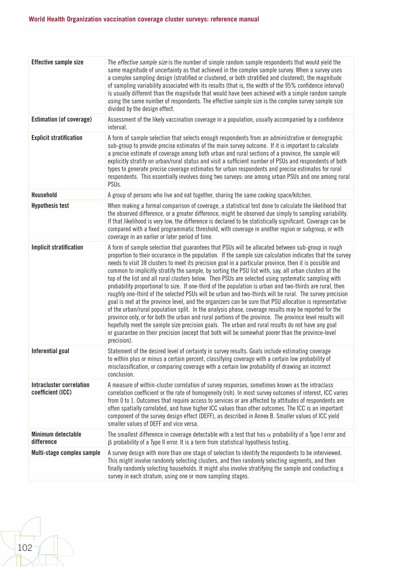
World Health Organization vaccination coverage cluster surveys: reference manual
102
Effective sample size The effective sample size is the number of simple random sample respondents that would yield the same magnitude of uncertainty as that achieved in the complex sample survey. When a survey uses a complex sampling design (stratified or clustered, or both stratified and clustered), the magnitude of sampling variability associated with its results (that is, the width of the 95% confidence interval) is usually different than the magnitude that would have been achieved with a simple random sample using the same number of respondents. The effective sample size is the complex survey sample size divided by the design effect.
Estimation (of coverage) Assessment of the likely vaccination coverage in a population, usually accompanied by a confidence interval.
Explicit stratification A form of sample selection that selects enough respondents from an administrative or demographic sub-group to provide precise estimates of the main survey outcome. If it is important to calculate a precise estimate of coverage among both urban and rural sections of a province, the sample will explicitly stratify on urban/rural status and visit a sufficient number of PSUs and respondents of both types to generate precise coverage estimates for urban respondents and precise estimates for rural respondents. This essentially involves doing two surveys: one among urban PSUs and one among rural PSUs.
Household A group of persons who live and eat together, sharing the same cooking space/kitchen.
Hypothesis test When making a formal comparison of coverage, a statistical test done to calculate the likelihood that the observed difference, or a greater difference, might be observed due simply to sampling variability. If that likelihood is very low, the difference is declared to be statistically significant. Coverage can be compared with a fixed programmatic threshold, with coverage in another region or subgroup, or with coverage in an earlier or later period of time.
Implicit stratification A form of sample selection that guarantees that PSUs will be allocated between sub-group in rough proportion to their occurance in the population. If the sample size calculation indicates that the survey needs to visit 38 clusters to meet its precision goal in a particular province, then it is possible and common to implicitly stratify the sample, by sorting the PSU list with, say, all urban clusters at the top of the list and all rural clusters below. Then PSUs are selected using systematic sampling with probability proportional to size. If one-third of the population is urban and two-thirds are rural, then roughly one-third of the selected PSUs will be urban and two-thirds will be rural. The survey precision goal is met at the province level, and the organizers can be sure that PSU allocation is representative of the urban/rural population split. In the analysis phase, coverage results may be reported for the province only, or for both the urban and rural portions of the province. The province level results will hopefully meet the sample size precision goals. The urban and rural results do not have any goal or guarantee on their precision (except that both will be somewhat poorer than the province-level precision).
Inferential goal Statement of the desired level of certainty in survey results. Goals include estimating coverage to within plus or minus a certain percent, classifying coverage with a certain low probability of misclassification, or comparing coverage with a certain low probability of drawing an incorrect conclusion.
Intracluster correlation coefficient (ICC)
A measure of within-cluster correlation of survey responses, sometimes known as the intraclass correlation coefficient or the rate of homogeneity (roh). In most survey outcomes of interest, ICC varies from 0 to 1. Outcomes that require access to services or are affected by attitudes of respondents are often spatially correlated, and have higher ICC values than other outcomes. The ICC is an important component of the survey design effect (DEFF), as described in Annex B. Smaller values of ICC yield smaller values of DEFF and vice versa.
Minimum detectable difference
The smallest difference in coverage detectable with a test that has probability of a Type I error and probability of a Type II error. It is a term from statistical hypothesis testing.
Multi-stage complex sample A survey design with more than one stage of selection to identify the respondents to be interviewed. This might involve randomly selecting clusters, and then randomly selecting segments, and then finally randomly selecting households. It might also involve stratifying the sample and conducting a survey in each stratum, using one or more sampling stages.
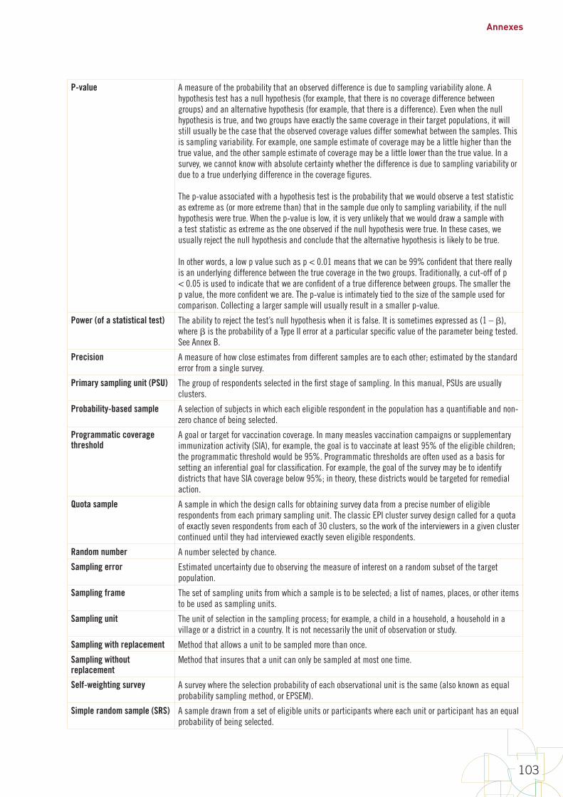
Annexes
103
P-value A measure of the probability that an observed difference is due to sampling variability alone. A hypothesis test has a null hypothesis (for example, that there is no coverage difference between groups) and an alternative hypothesis (for example, that there is a difference). Even when the null hypothesis is true, and two groups have exactly the same coverage in their target populations, it will still usually be the case that the observed coverage values differ somewhat between the samples. This is sampling variability. For example, one sample estimate of coverage may be a little higher than the true value, and the other sample estimate of coverage may be a little lower than the true value. In a survey, we cannot know with absolute certainty whether the difference is due to sampling variability or due to a true underlying difference in the coverage figures.
The p-value associated with a hypothesis test is the probability that we would observe a test statistic as extreme as (or more extreme than) that in the sample due only to sampling variability, if the null hypothesis were true. When the p-value is low, it is very unlikely that we would draw a sample with a test statistic as extreme as the one observed if the null hypothesis were true. In these cases, we usually reject the null hypothesis and conclude that the alternative hypothesis is likely to be true.
In other words, a low p value such as p < 0.01 means that we can be 99% confident that there really is an underlying difference between the true coverage in the two groups. Traditionally, a cut-off of p < 0.05 is used to indicate that we are confident of a true difference between groups. The smaller the p value, the more confident we are. The p-value is intimately tied to the size of the sample used for comparison. Collecting a larger sample will usually result in a smaller p-value.
Power (of a statistical test) The ability to reject the test’s null hypothesis when it is false. It is sometimes expressed as (1 – ), where is the probability of a Type II error at a particular specific value of the parameter being tested. See Annex B.
Precision A measure of how close estimates from different samples are to each other; estimated by the standard error from a single survey.
Primary sampling unit (PSU) The group of respondents selected in the first stage of sampling. In this manual, PSUs are usually clusters.
Probability-based sample A selection of subjects in which each eligible respondent in the population has a quantifiable and non-zero chance of being selected.
Programmatic coverage threshold
A goal or target for vaccination coverage. In many measles vaccination campaigns or supplementary immunization activity (SIA), for example, the goal is to vaccinate at least 95% of the eligible children; the programmatic threshold would be 95%. Programmatic thresholds are often used as a basis for setting an inferential goal for classification. For example, the goal of the survey may be to identify districts that have SIA coverage below 95%; in theory, these districts would be targeted for remedial action.
Quota sample A sample in which the design calls for obtaining survey data from a precise number of eligible respondents from each primary sampling unit. The classic EPI cluster survey design called for a quota of exactly seven respondents from each of 30 clusters, so the work of the interviewers in a given cluster continued until they had interviewed exactly seven eligible respondents.
Random number A number selected by chance.
Sampling error Estimated uncertainty due to observing the measure of interest on a random subset of the target population.
Sampling frame The set of sampling units from which a sample is to be selected; a list of names, places, or other items to be used as sampling units.
Sampling unit The unit of selection in the sampling process; for example, a child in a household, a household in a village or a district in a country. It is not necessarily the unit of observation or study.
Sampling with replacement Method that allows a unit to be sampled more than once.
Sampling without replacement
Method that insures that a unit can only be sampled at most one time.
Self-weighting survey A survey where the selection probability of each observational unit is the same (also known as equal probability sampling method, or EPSEM).
Simple random sample (SRS) A sample drawn from a set of eligible units or participants where each unit or participant has an equal probability of being selected.

World Health Organization vaccination coverage cluster surveys: reference manual
104
Single-stage cluster sample A sample in which clusters are selected randomly, and within each selected cluster, every eligible respondent is interviewed.
Statistical significance The standard by which results are judged as being likely due or not due to chance.
Stratum (plural: strata) and stratification
The word stratum can mean different things in different contexts, and there are several methods of stratification. In this entry we use the example of urban and rural residents as two sub-populations of interest. The points below would be equally applicable with many other demographic characteristics.
In the sample size calculation and sample design phase of a survey, a stratum is portion of the population for which survey results will be estimated and reported with a desired level of precision on the survey's primary outcome (the sample size has been purposefully selected to be large enough to do this). We say that a survey is stratified if the eligible respondents are divided into mutually exclusive and exhaustive groups, and a separate survey is conducted and reported for several or all groups. Coverage surveys are often explicitly stratified geographically (e.g., visiting enough PSUs in each province to generate a precise coverage estimate for every province - see the Annex A entry titled Explicit Stratification). Within each province it is possible to further explicitly stratify by urban/rural status, selecting enough urban PSUs and enough rural PSUs to generate precise coverage estimates among both groups. This is possible, but not common in WHO coverage surveys. The more common practice is to explicitly stratify on geographic areas and then to implicitly stratify the sample within each province based on a demographic characteristic, like urban and rural population. (See the Annex A entry titled Implicit Stratification.) Separate results may be reported for coverage among urban vs rural portions of the province in both situations: whether the survey uses explicit or implicit urban/rural stratification. Explicit stratification may sound desirable but it requires additional costs, resources, time and sample size.
A third possibility would be to select PSUs without consideration or regard for urban/rural status. In that case the analysis would require additional weighting and assumptions in order to generate meaninful coverage estimates for both the urban and rural portion of the province.
When the survey is conducted in every stratum, it is possible to aggregate the data (or results) across strata, with care, to estimate overall results. For example, we can combine data across all provinces, weighting appropriately, to estimate representative national level coverage figures. In some situations, eligible respondents are divided into groups, and surveys are only conducted in a subset of those groups (for example, only in provinces thought to have especially low coverage). It may not be possible to combine data across the subset of strata that were selected purposefully (that is, not selected randomly) to estimate national level results.
Supplementary immunization activity/ activities (SIA)
Any immunization activity conducted in addition to routine immunization services.
Survey weight A value that indicates how much each record or case will count in a statistical procedure. Each record in a survey dataset might be accompanied by one or more survey weights, to indicate how many population level eligible respondents are represented by the respondent in the sample. A statistician calculates the weights in what is usually a multi-step process, as described in Annex J.
Two-stage cluster sample A sample in which clusters are selected randomly, and then within each selected cluster, a second stage of sampling occurs in which a subset of eligible respondents is selected to be interviewed.
Type I error A term from statistical hypothesis testing: to incorrectly reject the null hypothesis. In study design we limit the probability of Type I errors by setting an explicit (usually low) value of the parameter designated (alpha). It is common to set =0.05 or 5%.
Type II error A term from statistical hypothesis testing: to incorrectly fail to reject the null hypothesis. In study design we limit the probability of Type II errors at some value of the parameter being tested, by setting an explicit value of the parameter designated (beta). Note that 1- equals the statistical power of the test at that value of the parameter.
Vaccination coverage The proportion of individuals in the target population who are vaccinated.
Vaccination coverage target A goal that is prepared for a health facility, stating that states what proportion of individuals in the target population will be vaccinated with specific vaccines in a given time period.
Valid dose A dose that was administered when a child had reached the minimum age for the vaccine, and was administered with the proper spacing between doses according to the national schedule.
Weight A number that expresses the relative number of population units represented by a given sampled unit.
Annexes
105
Annex B1: Steps to calculate a cluster survey sample size for estimation or classification
This annex is the first of three that explain how to calculate the right sample size to meet the survey goals. These three annexes contain the following information: 1. Annex B1 describes six steps to calculate a cluster survey sample size for either coverage estimation or classification
purposes. Along the way, the accompanying tables and equations will help readers to calculate several factors, labelled A through E, which may be multiplied together to calculate the target total number of respondents, number of clusters, and number of households to visit, in order to achieve a total survey sample size that will meet the inferential goals of the survey.
2. Annex B2 provides equations for extending the tables in Annex B1. Some readers may wish to understand more precisely how the tables were constructed; they may wish to work through the equations themselves. Other readers may encounter situations with unusual design parameters; the equations in Annex B2 will facilitate extending the tables to include these situations.
3. Annex B3 addresses the less common inferential goal of designing a survey to be well powered to detect differences in coverage – either differences over time or differences between subgroups. This is usually not the primary goal of a vaccination coverage survey but can be an important secondary goal. The tables and equations will help the reader understand the sample sizes needed to conduct formal statistical hypothesis tests to compare coverage.
B1.1 Changes to the 2005 sample size guidance This manual recommends using updated Expanded Programme on Immunization (EPI) survey methods to assess vaccination coverage. We favour using larger samples to estimate coverage precisely, and smaller samples to classify coverage, using a weighted probability sample. Therefore, use the guidance included in this updated manual to calculate cluster survey sample sizes, rather than using Appendix C of the 2005 Immunization Coverage Cluster Survey: Reference Manual. Specifically, the sample size guidance in the 2005 manual had the following weaknesses:
1. The 2005 manual assumes that every survey will have a design effect of 2, regardless of the number of respondents per cluster. This is misleading. The design effect is a function of the intracluster correlation coefficient (ICC), the number of respondents per cluster, and the coefficient of variation of the sampling weights (CVw). Survey organizers do not have any control over the ICC, so if they change the design to include more respondents per cluster, the design effect gets larger. It does not remain constant across designs. This means that Tables C1, C2, and C3 of the 2005 manual are not correct, and should not be used.
2. In tests for changes in coverage over time, the 2005 manual assumes that the coverage at the earlier time is given, and was measured precisely with no uncertainty. This is never the case in practice. The earlier coverage will have been estimated using a survey, so there will be a degree of uncertainty due to sampling variability. This means that Table C4 of the 2005 manual is not correct and should not be used.
3. In Table C5, the 2005 manual assumes a 1-sided test when testing for a difference in coverage between places. This is not correct because a 2-sided test (which requires a larger sample size) is almost always the right thing to do when comparing coverage between two subgroups or places measured at the same time. It is common that before the survey, it is truly not known which subgroup has higher coverage, and therefore requires a 2-sided test. It is rare to have strong grounds for believing that one subgroup has higher coverage than another, so the 2-sided test is a more conservative approach.
For these reasons, we strongly recommend using the tables and equations in this updated reference manual. As always, if you have questions, we recommend consulting a sampling statistician during the design and analysis phases of a survey.
A Short Note on Sample Size Guidance in this 2018 Reference Manual
The sample size guidance in this annex has been updated to address the issues listed above, and to be consistent with sample size advice from a single modern source: Statistical Methods for Rates and Proportions (Third Edition, 2003) by Joseph L. Fleiss, Bruce Levin, Myunghee Cho Paik. This annex refers to specific equations and pages in that text.
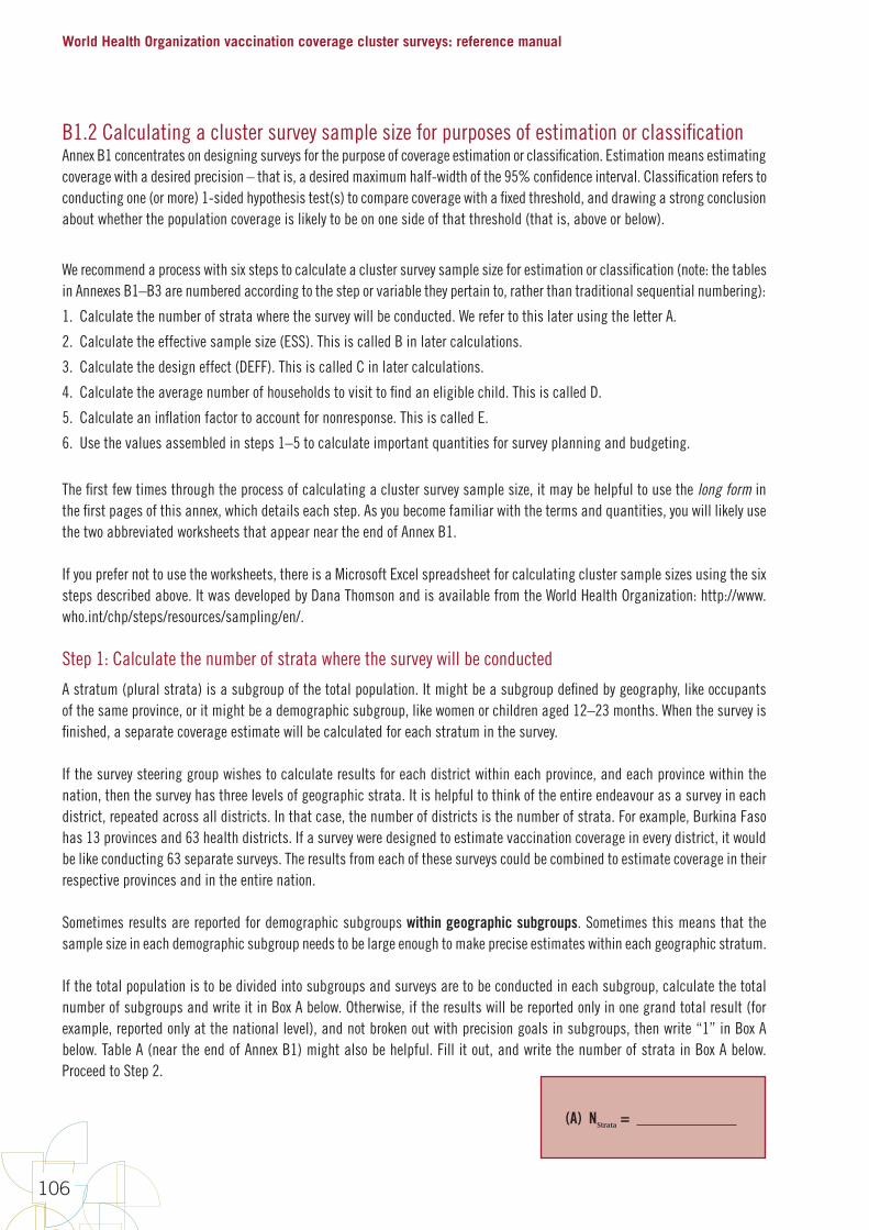
World Health Organization vaccination coverage cluster surveys: reference manual
106
B1.2 Calculating a cluster survey sample size for purposes of estimation or classificationAnnex B1 concentrates on designing surveys for the purpose of coverage estimation or classification. Estimation means estimating coverage with a desired precision – that is, a desired maximum half-width of the 95% confidence interval. Classification refers to conducting one (or more) 1-sided hypothesis test(s) to compare coverage with a fixed threshold, and drawing a strong conclusion about whether the population coverage is likely to be on one side of that threshold (that is, above or below).
We recommend a process with six steps to calculate a cluster survey sample size for estimation or classification (note: the tables in Annexes B1–B3 are numbered according to the step or variable they pertain to, rather than traditional sequential numbering):
1. Calculate the number of strata where the survey will be conducted. We refer to this later using the letter A.
2. Calculate the effective sample size (ESS). This is called B in later calculations.
3. Calculate the design effect (DEFF). This is called C in later calculations.
4. Calculate the average number of households to visit to find an eligible child. This is called D.
5. Calculate an inflation factor to account for nonresponse. This is called E.
6. Use the values assembled in steps 1–5 to calculate important quantities for survey planning and budgeting.
The first few times through the process of calculating a cluster survey sample size, it may be helpful to use the long form in the first pages of this annex, which details each step. As you become familiar with the terms and quantities, you will likely use the two abbreviated worksheets that appear near the end of Annex B1.
If you prefer not to use the worksheets, there is a Microsoft Excel spreadsheet for calculating cluster sample sizes using the six steps described above. It was developed by Dana Thomson and is available from the World Health Organization: http://www.who.int/chp/steps/resources/sampling/en/.
Step 1: Calculate the number of strata where the survey will be conducted
A stratum (plural strata) is a subgroup of the total population. It might be a subgroup defined by geography, like occupants of the same province, or it might be a demographic subgroup, like women or children aged 12–23 months. When the survey is finished, a separate coverage estimate will be calculated for each stratum in the survey.
If the survey steering group wishes to calculate results for each district within each province, and each province within the nation, then the survey has three levels of geographic strata. It is helpful to think of the entire endeavour as a survey in each district, repeated across all districts. In that case, the number of districts is the number of strata. For example, Burkina Faso has 13 provinces and 63 health districts. If a survey were designed to estimate vaccination coverage in every district, it would be like conducting 63 separate surveys. The results from each of these surveys could be combined to estimate coverage in their respective provinces and in the entire nation.
Sometimes results are reported for demographic subgroups within geographic subgroups. Sometimes this means that the sample size in each demographic subgroup needs to be large enough to make precise estimates within each geographic stratum.
If the total population is to be divided into subgroups and surveys are to be conducted in each subgroup, calculate the total number of subgroups and write it in Box A below. Otherwise, if the results will be reported only in one grand total result (for example, reported only at the national level), and not broken out with precision goals in subgroups, then write “1” in Box A below. Table A (near the end of Annex B1) might also be helpful. Fill it out, and write the number of strata in Box A below. Proceed to Step 2.
(A) NStrata
=

Annexes
107
Step 2: Calculate the effective sample size (ESS)
Although cluster samples require a larger total sample size than simple random samples, cluster samples are less expensive than simple random samples. This is because they require field staff to visit fewer locations, and staff can collect data from several respondents per location.
This step calculates the number of survey respondents required in order to meet the inferential goal of the survey, if a simple random sample of respondents were done. In later steps, this is called the effective sample size (ESS) and will be inflated to account for the clustering effect.
First, decide whether you wish to calculate precise results in each stratum (requiring higher sample sizes), or whether less precise results are adequate at the lowest level of stratum (for example, districts) as long as the results are quite precise when aggregated at the province and national levels.
Do you require very precise results for each stratum?
Circle answer: YES / NO
If yes, complete the section titled “Calculating ESS for estimating coverage”. If no, complete the section titled “Calculating ESS for classifying coverage”. If an inferential goal of the survey is to compare results from two surveys (such as over time or between two places), read Annex B3 to obtain the ESS for each of the two surveys, and write both values in Box B below.
Calculating ESS for estimating coverage
If results are to be estimated to within a given precision level at the lowest level of strata (for example, districts), specify the expected coverage level for the vaccine or other measure of most interest, and the precision with which the coverage should be estimated. Write those values below:
Expected coverage: %
Desired precision level: ± %
If you are estimating coverage for several equally important measures, write in the expected coverage for the measure that is likely to be nearest 50% coverage. Use Table B-1 (near the end of Annex B1) to look up the ESS based on your expected coverage and desired precision level. For example, if the outcome of interest is the third dose of a DTP-containing vaccine (DTPCV3), expected coverage is 75%. To have precision of ± 5%, Table B-1 indicates that ESS = 340.

World Health Organization vaccination coverage cluster surveys: reference manual
108
Write the ESS in Box B below. Proceed to Step 3.
(B) ESS =
Calculating ESS for classifying coverage
If sufficient resources are not available to obtain very precise results in every stratum, it can be helpful to select a sample size based on its power to classify coverage in those strata as being higher or lower than a fixed programmatic threshold. The results will be a coverage point estimate and confidence region, and coverage will either be:
• very likely lower than the programmatic threshold,
• very likely higher than the threshold, or
• not distinguishable from the threshold with high confidence using the sample size in this survey.
To select the effective sample size, identify the threshold of interest and then specify the desired likelihood that the survey correctly classifies strata whose coverage falls a certain distance above or below that threshold. Of course, it would be nice to correctly classify strata 100% of the time, but it is difficult to guarantee because of sampling variability: some samples of respondents will yield many vaccinated children, while other samples of the same size, collected in a similarly random fashion, will by chance yield fewer vaccinated children. That is the nature of sampling. Although we cannot guarantee that a small sample will correctly classify every stratum, we can select a sample size that is very likely to make correct classifications when coverage is a specified distance above or below the threshold. This design principle is similar to that used in lot quality assurance sampling (LQAS), but the results here are likely to be clearer than those from clustered LQAS.
This design requires the following five input parameters to be specified in order to look up the corresponding ESS:
1. The programmatic threshold is a coverage level of interest. It might be the coverage target.
2. Delta s a coverage percent defining a distance from the programmatic threshold. If the true coverage is at least delta points away from the programmatic threshold, we choose a sample size likely to classify those districts as having coverage that is likely different than delta.
For example, if the programmatic threshold is 80% and delta is 15%, then when coverage is below 65% (80 – 15) you want the survey results to be very likely to show that coverage is very likely lower than 80%. Similarly, when coverage is above 95% (80 + 15) you want the survey results to be very likely to show that coverage is very likely above 80%.
3. Direction indicates whether you are specifying the statistical power for correctly classifying strata with coverage delta percent above the programmatic threshold, or delta percent below the programmatic threshold. If the threshold of interest is 80% and you want to be very sure to correctly classify strata with coverage above 90%, then the direction is above and you should use Table B-3 to look up the ESS. If the direction is below then use Table B-2. Note that the effective sample sizes in B-2 are larger than those in B-3, so the conservative choice is to use Table B-2 unless your primary focus is detecting differences above the programmatic threshold.
4. Alpha () is the probability that a stratum with true population coverage at the programmatic threshold will be mistakenly classified as very likely to be above or below that threshold.
5. Beta () is the probability that a stratum with true population coverage delta points away from the threshold (Table B-2 for below and Table B-3 for above) will be mistakenly classified as having coverage not different than the threshold. The quantity 100% – is the statistical power of the classifier.
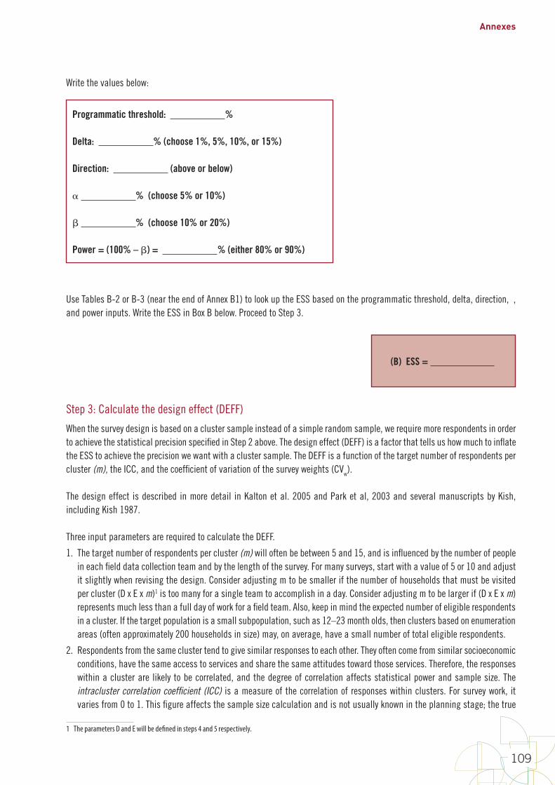
Annexes
109
Write the values below:
Programmatic threshold: %
Delta: % (choose 1%, 5%, 10%, or 15%)
Direction: (above or below)
% (choose 5% or 10%)
% (choose 10% or 20%)
Power = (100% – ) = % (either 80% or 90%)
Use Tables B-2 or B-3 (near the end of Annex B1) to look up the ESS based on the programmatic threshold, delta, direction, α, and power inputs. Write the ESS in Box B below. Proceed to Step 3.
(B) ESS =
Step 3: Calculate the design effect (DEFF)
When the survey design is based on a cluster sample instead of a simple random sample, we require more respondents in order to achieve the statistical precision specified in Step 2 above. The design effect (DEFF) is a factor that tells us how much to inflate the ESS to achieve the precision we want with a cluster sample. The DEFF is a function of the target number of respondents per cluster (m), the ICC, and the coefficient of variation of the survey weights (CVw).
The design effect is described in more detail in Kalton et al. 2005 and Park et al, 2003 and several manuscripts by Kish, including Kish 1987.
Three input parameters are required to calculate the DEFF.
1. The target number of respondents per cluster (m) will often be between 5 and 15, and is influenced by the number of people in each field data collection team and by the length of the survey. For many surveys, start with a value of 5 or 10 and adjust it slightly when revising the design. Consider adjusting m to be smaller if the number of households that must be visited per cluster (D x E x m)1 is too many for a single team to accomplish in a day. Consider adjusting m to be larger if (D x E x m) represents much less than a full day of work for a field team. Also, keep in mind the expected number of eligible respondents in a cluster. If the target population is a small subpopulation, such as 12–23 month olds, then clusters based on enumeration areas (often approximately 200 households in size) may, on average, have a small number of total eligible respondents.
2. Respondents from the same cluster tend to give similar responses to each other. They often come from similar socioeconomic conditions, have the same access to services and share the same attitudes toward those services. Therefore, the responses within a cluster are likely to be correlated, and the degree of correlation affects statistical power and sample size. The intracluster correlation coefficient (ICC) is a measure of the correlation of responses within clusters. For survey work, it varies from 0 to 1. This figure affects the sample size calculation and is not usually known in the planning stage; the true
1 The parameters D and E will be defined in steps 4 and 5 respectively.
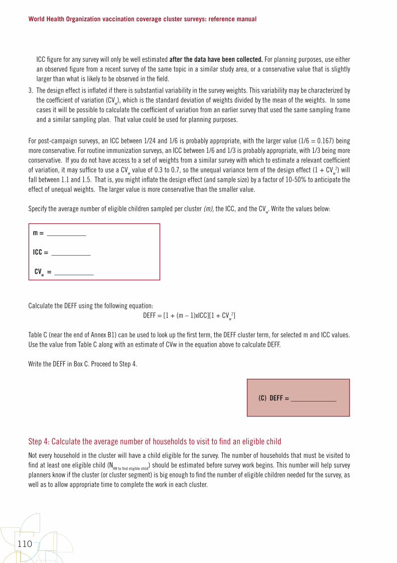
World Health Organization vaccination coverage cluster surveys: reference manual
110
ICC figure for any survey will only be well estimated after the data have been collected. For planning purposes, use either an observed figure from a recent survey of the same topic in a similar study area, or a conservative value that is slightly larger than what is likely to be observed in the field.
3. The design effect is inflated if there is substantial variability in the survey weights. This variability may be characterized by the coefficient of variation (CVw), which is the standard deviation of weights divided by the mean of the weights. In some cases it will be possible to calculate the coefficient of variation from an earlier survey that used the same sampling frame and a similar sampling plan. That value could be used for planning purposes.
For post-campaign surveys, an ICC between 1/24 and 1/6 is probably appropriate, with the larger value (1/6 = 0.167) being more conservative. For routine immunization surveys, an ICC between 1/6 and 1/3 is probably appropriate, with 1/3 being more conservative. If you do not have access to a set of weights from a similar survey with which to estimate a relevant coefficient of variation, it may suffice to use a CVw value of 0.3 to 0.7, so the unequal variance term of the design effect (1 + CVw
2) will fall between 1.1 and 1.5. That is, you might inflate the design effect (and sample size) by a factor of 10-50% to anticipate the effect of unequal weights. The larger value is more conservative than the smaller value.
Specify the average number of eligible children sampled per cluster (m), the ICC, and the CVw. Write the values below:
m =
ICC =
CVw =
Calculate the DEFF using the following equation:DEFF = [1 + (m – 1)xICC][1 + CVw
2]
Table C (near the end of Annex B1) can be used to look up the first term, the DEFF cluster term, for selected m and ICC values. Use the value from Table C along with an estimate of CVw in the equation above to calculate DEFF.
Write the DEFF in Box C. Proceed to Step 4.
(C) DEFF =
Step 4: Calculate the average number of households to visit to find an eligible child
Not every household in the cluster will have a child eligible for the survey. The number of households that must be visited to find at least one eligible child (NHH to find eligible child) should be estimated before survey work begins. This number will help survey planners know if the cluster (or cluster segment) is big enough to find the number of eligible children needed for the survey, as well as to allow appropriate time to complete the work in each cluster.

Annexes
111
If NHH to find eligible child is known or easily found from recent census or survey data, that number should be written in Box D below, and the reader can proceed to Step 5. If it is not known, it can be estimated in various ways. Birth rates, infant mortality rates, and household size are some variables that may be easy to obtain from recent census or survey data to help estimate NHH to find eligible child. Consider the following equations. Equation B1-1 estimates NSurvived at birth per HH, which is used in Equation B1-2 to estimate NHH to find eligible child.
Equation B1-1 and B1-2:
B1-9
Step 4: Calculate the average number of households to visit to find an eligible child Noteveryhouseholdintheclusterwillhaveachildeligibleforthesurvey.Thenumberofhouseholdsthatmustbevisitedtofindatleastoneeligiblechild(NHHtofindeligiblechild)shouldbeestimatedbeforesurveyworkbegins.Thisnumberwillhelpsurveyplannersknowifthecluster(orclustersegment)isbigenoughtofindthenumberofeligiblechildrenneededforthesurvey,aswellastoallowappropriatetimetocompletetheworkineachcluster.
IfNHHtofindeligiblechildisknownoreasilyfoundfromrecentcensusorsurveydata,thatnumbershouldbewritteninBoxDbelow,andthereadercanproceedtoStep5.Ifitisnotknown,itcanbeestimatedinvariousways.Birthrates,infantmortalityrates,andhouseholdsizearesomevariablesthatmaybeeasytoobtainfromrecentcensusorsurveydatatohelpestimateNHHtofindeligiblechild.Considerthefollowingequations.EquationB1-1estimatesNSurvivedatbirthperHH,whichisusedinEquationB1-2toestimateNHHtofindeligiblechild.
!"#$%&%'(*+,&$+-.'$// = 12345
(78889:
)<=>>>?@A
=>>>(B1-1)
!//+BC&D('E&F&,E'G-&E( ==
H:IJKLKMNOPQLJPRSMJ99(B1-2)
YCisthenumberofyearsofeligiblechildreninthecohort,BRisthebirthrateper1000population,HSistheaveragehouseholdsize,andIMistheinfantmortalityrateper1000livebirths.ThefirstterminEquationB1-1estimatesthenumberoflivebirthsperhousehold,andthesecondtermestimatestheproportionoflivebirthsthatsurvivedtotheirfirstbirthday.ThemultiplierYCassumeseveryonesurvivesaftertheirfirstbirthday,soEquationB1-2underestimatesNHHtofindeligiblechild.RoundtheresultfromEquationB1-2uptothenearestwholenumber.Example1:SupposeasurveyisscheduledtooccurinEthiopiaestimatingcoveragelevelsforasingleyearcohort,children12–23months.Inthe2011EthiopiaDemographicHealthSurvey,thebirthrateper1000populationwasestimatedtobe34.5,theinfantmortalityrateper1000livebirthswasestimatedtobe59,andtheaveragehouseholdsizewasestimatedtobe4.6.Thenumberofyearsofeligiblechildreninthecohortis1.UsingEquationsB1-1andB1-2:
!"#$%&%'(*+,&$+-.'$// = 1<34.5
(10004.6 )
<1000 − 591000
= 0.149
!//+BC&D('E&F&,E'G-&E( =1
0.149= 6.7
Anestimated1inevery7householdswillhaveaneligiblechildforthissurvey.Example2:InExample1,ifthecohortofinterestwasfor1–5yearolds,thenYC=5–1=4andEquationsB1-1andB1-2yield:
YC is the number of years of eligible children in the cohort, BR is the birth rate per 1000 population, HS is the average household size, and IM is the infant mortality rate per 1000 live births. The first term in Equation B1-1 estimates the number of live births per household, and the second term estimates the proportion of live births that survived to their first birthday. The multiplier YC assumes everyone survives after their first birthday, so Equation B1-2 underestimates NHH to find eligible child. Round the result from Equation B1-2 up to the nearest whole number.
Example 1: Suppose a survey is scheduled to occur in Ethiopia estimating coverage levels for a single year cohort, children 12–23 months. In the 2011 Ethiopia Demographic Health Survey, the birth rate per 1000 population was estimated to be 34.5, the infant mortality rate per 1000 live births was estimated to be 59, and the average household size was estimated to be 4.6. The number of years of eligible children in the cohort is 1. Using Equations B1-1 and B1-2:
B1-9
Step 4: Calculate the average number of households to visit to find an eligible child Noteveryhouseholdintheclusterwillhaveachildeligibleforthesurvey.Thenumberofhouseholdsthatmustbevisitedtofindatleastoneeligiblechild(NHHtofindeligiblechild)shouldbeestimatedbeforesurveyworkbegins.Thisnumberwillhelpsurveyplannersknowifthecluster(orclustersegment)isbigenoughtofindthenumberofeligiblechildrenneededforthesurvey,aswellastoallowappropriatetimetocompletetheworkineachcluster.
IfNHHtofindeligiblechildisknownoreasilyfoundfromrecentcensusorsurveydata,thatnumbershouldbewritteninBoxDbelow,andthereadercanproceedtoStep5.Ifitisnotknown,itcanbeestimatedinvariousways.Birthrates,infantmortalityrates,andhouseholdsizearesomevariablesthatmaybeeasytoobtainfromrecentcensusorsurveydatatohelpestimateNHHtofindeligiblechild.Considerthefollowingequations.EquationB1-1estimatesNSurvivedatbirthperHH,whichisusedinEquationB1-2toestimateNHHtofindeligiblechild.
!"#$%&%'(*+,&$+-.'$// = 12345
(78889:
)<=>>>?@A
=>>>(B1-1)
!//+BC&D('E&F&,E'G-&E( ==
H:IJKLKMNOPQLJPRSMJ99(B1-2)
YCisthenumberofyearsofeligiblechildreninthecohort,BRisthebirthrateper1000population,HSistheaveragehouseholdsize,andIMistheinfantmortalityrateper1000livebirths.ThefirstterminEquationB1-1estimatesthenumberoflivebirthsperhousehold,andthesecondtermestimatestheproportionoflivebirthsthatsurvivedtotheirfirstbirthday.ThemultiplierYCassumeseveryonesurvivesaftertheirfirstbirthday,soEquationB1-2underestimatesNHHtofindeligiblechild.RoundtheresultfromEquationB1-2uptothenearestwholenumber.Example1:SupposeasurveyisscheduledtooccurinEthiopiaestimatingcoveragelevelsforasingleyearcohort,children12–23months.Inthe2011EthiopiaDemographicHealthSurvey,thebirthrateper1000populationwasestimatedtobe34.5,theinfantmortalityrateper1000livebirthswasestimatedtobe59,andtheaveragehouseholdsizewasestimatedtobe4.6.Thenumberofyearsofeligiblechildreninthecohortis1.UsingEquationsB1-1andB1-2:
!"#$%&%'(*+,&$+-.'$// = 1<34.5
(10004.6 )
<1000 − 591000
= 0.149
!//+BC&D('E&F&,E'G-&E( =1
0.149= 6.7
Anestimated1inevery7householdswillhaveaneligiblechildforthissurvey.Example2:InExample1,ifthecohortofinterestwasfor1–5yearolds,thenYC=5–1=4andEquationsB1-1andB1-2yield:
An estimated 1 in every 7 households will have an eligible child for this survey.
Example 2: In Example 1, if the cohort of interest was for 1–5 year olds, then YC = 5 – 1 = 4 and Equations B1-1 and B1-2 yield:
B1-10
!"#$%&%'(*+,&$+-.'$// = 4<34.5
(10004.6 )
<1000 − 591000
= 0.6
!//+BC&D('E&F&,E'G-&E( =10.6
= 1.67Expandingthebirthcohorttranslatestomorehouseholdswithaneligiblechildforthesurvey.Inthisexample,anaverageoftwohouseholdswouldneedtobevisitedtofindaneligiblechild.Example3:InExample1,ifthebirthcohortwasfor1–15yearolds,thenYC=15–1=14andEquationsB1-1andB1-2yield:
!"#$%&%'(*+,&$+-.'$// = 14<34.510004.6
<1000 − 591000
= 2.09
!__`abcdefgchcigfjℎcge =1
2.09=0.48
Expandingthebirthcohortdramaticallytranslatestoevenmorehouseholdswithaneligiblechildforthesurvey.Inthisexample,everyhouseholdisestimatedtohaveaneligiblechild.UsingEquationsB1-1andB1-2,estimateNHHtofindeligiblechildandwriteitinBoxDbelow.ConsultastatisticianorthecensusbureauiftheratesusedinEquationsB1-1andB1-2arenotknownornotwellestimated,andifadifferentwaytoestimateNHHtofindeligiblechildisneeded.Discussionswithcolleagueswhohaverecentlycompletednationalchildhealthsurveys(malaria,nutrition,etc.)mayalsobehelpful.
(D)NHHtofindeligiblechild=__________
Expanding the birth cohort translates to more households with an eligible child for the survey. In this example, an average of two households would need to be visited to find an eligible child.
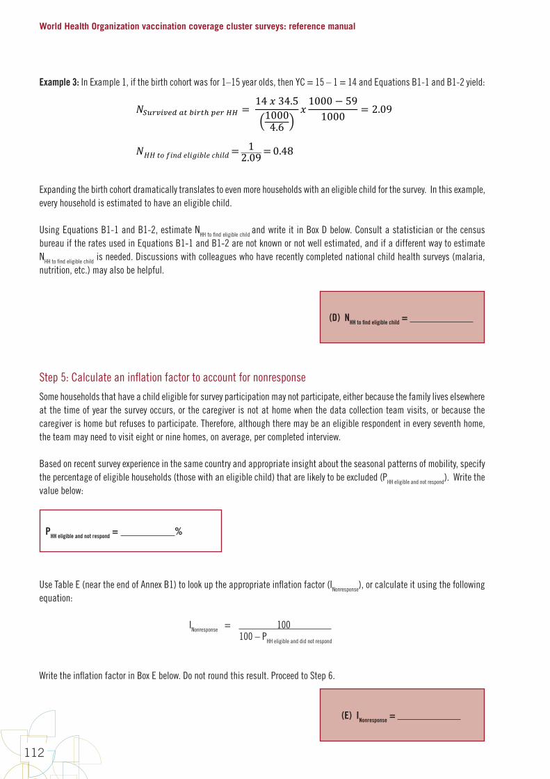
World Health Organization vaccination coverage cluster surveys: reference manual
112
Example 3: In Example 1, if the birth cohort was for 1–15 year olds, then YC = 15 – 1 = 14 and Equations B1-1 and B1-2 yield:
B1-10
!"#$%&%'(*+,&$+-.'$// = 4<34.5
(10004.6 )
<1000 − 591000
= 0.6
!//+BC&D('E&F&,E'G-&E( =10.6
= 1.67Expandingthebirthcohorttranslatestomorehouseholdswithaneligiblechildforthesurvey.Inthisexample,anaverageoftwohouseholdswouldneedtobevisitedtofindaneligiblechild.Example3:InExample1,ifthebirthcohortwasfor1–15yearolds,thenYC=15–1=14andEquationsB1-1andB1-2yield:
!"#$%&%'(*+,&$+-.'$// = 14<34.510004.6
<1000 − 591000
= 2.09
!__`abcdefgchcigfjℎcge =1
2.09=0.48
Expandingthebirthcohortdramaticallytranslatestoevenmorehouseholdswithaneligiblechildforthesurvey.Inthisexample,everyhouseholdisestimatedtohaveaneligiblechild.UsingEquationsB1-1andB1-2,estimateNHHtofindeligiblechildandwriteitinBoxDbelow.ConsultastatisticianorthecensusbureauiftheratesusedinEquationsB1-1andB1-2arenotknownornotwellestimated,andifadifferentwaytoestimateNHHtofindeligiblechildisneeded.Discussionswithcolleagueswhohaverecentlycompletednationalchildhealthsurveys(malaria,nutrition,etc.)mayalsobehelpful.
(D)NHHtofindeligiblechild=__________
Expanding the birth cohort dramatically translates to even more households with an eligible child for the survey. In this example, every household is estimated to have an eligible child.
Using Equations B1-1 and B1-2, estimate NHH to find eligible child and write it in Box D below. Consult a statistician or the census bureau if the rates used in Equations B1-1 and B1-2 are not known or not well estimated, and if a different way to estimate NHH to find eligible child is needed. Discussions with colleagues who have recently completed national child health surveys (malaria, nutrition, etc.) may also be helpful.
(D) NHH to find eligible child =
Step 5: Calculate an inflation factor to account for nonresponse
Some households that have a child eligible for survey participation may not participate, either because the family lives elsewhere at the time of year the survey occurs, or the caregiver is not at home when the data collection team visits, or because the caregiver is home but refuses to participate. Therefore, although there may be an eligible respondent in every seventh home, the team may need to visit eight or nine homes, on average, per completed interview.
Based on recent survey experience in the same country and appropriate insight about the seasonal patterns of mobility, specify the percentage of eligible households (those with an eligible child) that are likely to be excluded (PHH eligible and not respond). Write the value below:
PHH eligible and not respond = %
Use Table E (near the end of Annex B1) to look up the appropriate inflation factor (INonresponse), or calculate it using the following equation:
INonresponse = 100 100 – PHH eligible and did not respond
Write the inflation factor in Box E below. Do not round this result. Proceed to Step 6.
(E) INonresponse =

Annexes
113
Step 6: Use the values above to calculate quantities needed for survey planning and budgeting
Copy the quantities A–E and m from the earlier sheets into these boxes:
A. NStrata
B. ESS
C. DEFF
D. NHH to find eligible child
E. INonresponse
m (from Step 3)
1. Calculate the total completed interviews needed (Ncs):
Ncs = X X = (A) (B) (C)
2. Using Ncs just calculated, and (D) and (E) in the boxes above, calculate the total number of households to visit to get the necessary completed interviews:
NHH to visit = X X = (Ncs) (D) (E)
3. Using (B) through (E) in the boxes above, calculate the target number of households to visit in each stratum:
NHH to visit per stratum = X X X = (B) (C) (D) (E)
4. Using (B) (C) and m, calculate the number of clusters needed per stratum:
Nclusters per stratum = X / = (B) (C) m
5. Calculate the total households to visit per cluster:
NHH per cluster = X X = (D) (E) m
6. Calculate the total number of clusters in the survey:
Nclusters total = X = (A) Nclusters per stratum
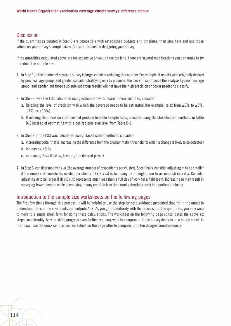
World Health Organization vaccination coverage cluster surveys: reference manual
114
DiscussionIf the quantities calculated in Step 6 are compatible with established budgets and timelines, then stop here and use those values as your survey’s sample sizes. Congratulations on designing your survey!
If the quantities calculated above are too expensive or would take too long, there are several modifications you can make to try to reduce the sample size.
1. In Step 1, if the number of strata to survey is large, consider reducing this number. For example, if results were originally desired by province, age group, and gender, consider stratifying only by province. You can still summarize the analysis by province, age group, and gender, but those sub-sub-subgroup results will not have the high precision or power needed to classify.
2. In Step 2, was the ESS calculated using estimation with desired precision? If so, consider:
a. Relaxing the level of precision with which the coverage needs to be estimated (for example, relax from ±3% to ±5%, ±7%, or ±10%).
b. If relaxing the precision still does not produce feasible sample sizes, consider using the classification methods in Table B-2 instead of estimating with a desired precision level from Table B-1.
3. In Step 2, if the ESS was calculated using classification methods, consider:
a. increasing delta (that is, increasing the difference from the programmatic threshold for which a change is likely to be detected)
b. increasing alpha
c. increasing beta (that is, lowering the desired power)
4. In Step 3, consider modifying m (the average number of respondents per cluster). Specifically, consider adjusting m to be smaller if the number of households needed per cluster (D x E x m) is too many for a single team to accomplish in a day. Consider adjusting m to be larger if (D x E x m) represents much less than a full day of work for a field team. Increasing m may result in surveying fewer clusters while decreasing m may result in less time (and potentially cost) in a particular cluster.
Introduction to the sample size worksheets on the following pagesThe first few times through this process, it will be helpful to use the step-by-step guidance presented thus far in the annex to understand the sample size inputs and outputs A–E. As you gain familiarity with the process and the quantities, you may wish to move to a single sheet form for doing these calculations. The worksheet on the following page consolidates the above six steps considerably. As your skills progress even further, you may wish to compare multiple survey designs on a single sheet. In that case, use the quick comparison worksheet on the page after to compare up to ten designs simultaneously.
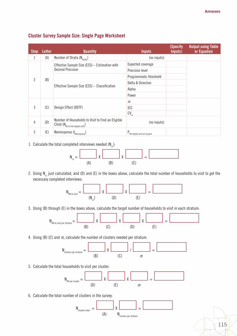
Annexes
115
Cluster Survey Sample Size: Single Page Worksheet
Step Letter Quantity Inputs(Specify Inputs)
Output using Table or Equation
1 (A) Number of Strata (NStrata) (no inputs)
2 (B)
Effective Sample Size (ESS) – Estimation with Desired Precision
Expected coverage
Precision level
Effective Sample Size (ESS) – Classification
Programmatic threshold
Delta & Direction
Alpha
Power
3 (C) Design Effect (DEFF)m
ICCCVw
4 (D) Number of Households to Visit to Find an Eligible Child (NHH to find eligible child)
(no inputs)
5 (E) Nonresponse (INonresponse) PHH eligible and not respond
1. Calculate the total completed interviews needed (Ncs):
Ncs = X X = (A) (B) (C)
2. Using Ncs just calculated, and (D) and (E) in the boxes above, calculate the total number of households to visit to get the necessary completed interviews:
NHH to visit = X X = (Ncs) (D) (E)
3. Using (B) through (E) in the boxes above, calculate the target number of households to visit in each stratum:
NHH to visit per stratum = X X X = (B) (C) (D) (E)
4. Using (B) (C) and m, calculate the number of clusters needed per stratum:
Nclusters per stratum = X / = (B) (C) m
5. Calculate the total households to visit per cluster:
NHH per cluster = X X = (D) (E) m
6. Calculate the total number of clusters in the survey:
Nclusters total = X = (A) Nclusters per stratum
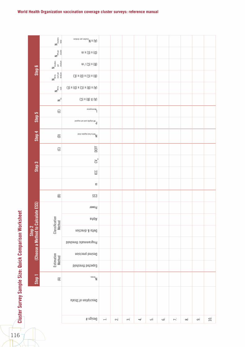
World Health Organization vaccination coverage cluster surveys: reference manual
116
Clus
ter S
urve
y Sa
mpl
e Si
ze: Q
uick
Com
paris
on W
orks
heet
Step
1St
ep 2
(C
hoos
e a
Met
hod
to C
alcu
late
ESS
)St
ep 3
Step
4St
ep 5
Step
6
(A)
Estim
atio
nM
etho
dCl
assi
ficat
ion
Met
hod
(B)
(C)
(D)
(E)
N cs
N HH to
vi
sit
N HH to
vi
sit p
er
stra
tum
N clus
ters
pe
r st
ratu
m
N HH p
er
clus
ter
N clus
ters
to
tal
Design #
Description of Strata
NStrata
Expected threshold
Desired precision
Programmatic threshold
Delta & direction
Alpha
Power
ESS
mIC
CCV
wDE
FF
NHH to find eligible child
PHH eligible and not respond
INonresponse
(A) X (B) x (C)
(A) x (B) x (C) x (D) x (E)
(B) x (C) x (D) x (E)
(B) x (C) / m
(D) x (E) x m
(A) x Nclusters per stratum
1. 2. 3. 4. 5. 6. 7. 8. 9. 10.
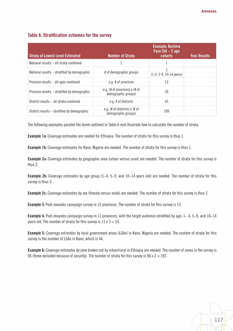
Annexes
117
Table A. Stratification schemes for the survey
Strata at Lowest Level Estimated Number of Strata
Example: Burkina Faso SIA – 3 age
cohorts Your Results
National results – all strata combined 1 1
National results – stratified by demographic # of demographic groups 3(1-4, 5-9, 10-14 years)
Province results – all ages combined e.g. # of provinces 13
Province results – stratified by demographic e.g. (# of provinces) x (# of demographic groups) 39
District results – all strata combined e.g. # of districts 63
District results – stratified by demographic e.g. (# of districts) x (# of demographic groups) 189
The following examples parallel the levels outlined in Table A and illustrate how to calculate the number of strata.
Example 1a: Coverage estimates are needed for Ethiopia. The number of strata for this survey is thus 1.
Example 1b: Coverage estimates for Kano, Nigeria are needed. The number of strata for this survey is thus 1.
Example 2a: Coverage estimates by geographic area (urban versus rural) are needed. The number of strata for this survey is thus 2.
Example 2b: Coverage estimates by age group (1–4, 5–9, and 10–14 years old) are needed. The number of strata for this survey is thus 3.
Example 2c: Coverage estimates by sex (female versus male) are needed. The number of strata for this survey is thus 2.
Example 3: Post-measles campaign survey in 13 provinces. The number of strata for this survey is 13.
Example 4: Post-measles campaign survey in 11 provinces, with the target audience stratified by age: 1– 4, 5–9, and 10–14 years old. The number of strata for this survey is 11 x 3 = 33.
Example 5: Coverage estimates by local government areas (LGAs) in Kano, Nigeria are needed. The number of strata for this survey is the number of LGAs in Kano, which is 44.
Example 6: Coverage estimates by zone broken out by urban/rural in Ethiopia are needed. The number of zones in the survey is 96 (three excluded because of security). The number of strata for this survey is 96 x 2 = 192.

World Health Organization vaccination coverage cluster surveys: reference manual
118
Table B-1. Effective sample size (ESS) by expected coverage and desired precision for the 95% confidence interval (CI)
Precision for 95% CI
Expected Coverage
5% 10% 15% 20% 25% 50-70% 75% 80% 85% 90% 95%
±3% 354 518 663 788 892 1,097 892 788 663 518 354
±4% 227 315 394 461 517 622 517 461 394 315 227
±5% 162 216 265 306 340 401 340 306 265 216 162
±6% 132 160 192 220 242 280 242 220 192 160 132
±7% 110 125 147 167 182 207 182 167 147 125 110
±8% 93 101 117 131 143 159 143 131 117 101 93
±9% 81 83 96 106 115 126 115 106 96 83 81
±10% 70 70 80 88 95 103 95 88 80 70 70
Note 1. These sample sizes are consistent with the sample size equations on page 35 of Fleiss, Levin, and Paik (2003), Statistical Methods for Rates and Proportions, 3rd edition, John Wiley & Sons, Inc., Hoboken, New Jersey. Note that within any row, the ESS does not change for coverage levels between 50% and 70%. This is not a mistake in the table, but rather a result of using a conservative upper bound of k = 1 in calculations for these values. As p moves away from 50%, k can be scaled down to something < 1 and a reduced sample size results.
Note 2. The values of ESS in Table B-1 have this property: If a survey sample has an ESS greater than or equal to the value in the table and if the estimated coverage is equal to the value at the top of the column, then neither side of a 95% Wilson confidence interval with continuity correction (the interval recommended in Fleiss et al.) will be longer than the precision listed at the left edge of the table. For example, see Figure B1-3 for a graphical depiction of the 95% CI when ESS = 70 and estimated coverage is 95%. Note that neither the short portion of the 95% CI (the upper portion in this case) nor the long portion of the 95% CI (the long portion is always the portion that points toward 50%) will be longer than 10%. If neither the upper nor lower portions are longer than 10%, then the two portions together will certainly not be longer than 20%.
Note 3. Recall from the 2005 EPI Cluster Survey Guidelines that when the design effect is 2, a sample of 30 x 7 = 210 will yield confidence intervals no wider than ±10%. The highest entry in this table for a precision of ± 10% is 103. If we multiple 103 by a design effect of 2, we obtain a total sample size per stratum of 206, which is essentially the same as 210. So Table B-1 is consistent with the 2005 EPI Cluster Survey Guidelines in that historically important respect.

Annexes
119
Note 4. For coverage between two values in the table, to be conservative, look up the ESS for the expected coverage that is closer to 50%. For example, if expected coverage is 73%, look up the ESS using 70%. If expected coverage is 23%, then look up the ESS using 25%.
Note 5. Table B-1 assumes that the population of eligible respondents is very large. When studying coverage in strata with small populations (for example, on a small island), it may be possible to achieve the desired precision with a smaller sample by incorporating a so-called finite population correction. Calculate the effective sample size using Table B-1 and estimate the total target population for the survey (N) (population of children aged 12–23 months in the stratum) and then calculate the revised
B1-‐20
Note 5. Table B-‐1 assumes that the population of eligible respondents is very large. When studying coverage in strata with small populations (for example, on a small island), it may be possible to achieve the desired precision with a smaller sample by incorporating a so-‐called finite population correction. Calculate the effective sample size using Table B-‐1 and estimate the total target population for the survey (N) (population of children aged 12–23 months in the stratum) and then calculate the revised ESS using the following formula: 𝐸𝐸𝑆𝑆𝑆𝑆′≥𝐸𝐸𝑆𝑆𝑆𝑆1+𝐸𝐸𝑆𝑆𝑆𝑆−1𝑁𝑁 Note that when the target population N is large compared with the ESS from Table B-‐1, then ESS’ (corrected effective sample size) will be essentially equal to ESS. But if ESS is an appreciable proportion of N then ESS’ will be smaller than ESS and the difference may result in a less expensive survey. Check with a sampling statistician; if the finite population correction is appropriate, use the value of ESS’ rather than ESS for the factor A in subsequent calculations in this annex. Note that if the finite population correction is used to determine sample size, it should also be incorporated into the analysis. Be sure to specify the right options in the analysis software to incorporate N into the calculations.
Figures B1-‐1 through B1-‐3 illustrate the 95% confidence intervals that would be achieved with 24 of the samples from Table B-‐1. Figure B1-‐1 shows eight estimated probability distributions where the sample proportion is 50%. Each distribution is truncated at the limits of the 95% confidence interval. The figure also shows the 95% upper confidence bound and 95% lower confidence bounds using small tick marks.
Figure B1-‐2 shows the comparable distributions that would result from samples where coverage was 80%, and Figure B1-‐3 shows comparable distributions for the designs from Table B-‐1 where sample coverage is 95%. Distributions with coverage >50% are asymmetric, with the longer tail pointing toward 50%. The figures show that the designs in Table B-‐1 achieve the precision goals specified along the vertical axis of the table.
using the following formula:
B1-18
Note5.TableB-1assumesthatthepopulationofeligiblerespondentsisverylarge.Whenstudyingcoverageinstratawithsmallpopulations(forexample,onasmallisland),itmaybepossibletoachievethedesiredprecisionwithasmallersamplebyincorporatingaso-calledfinitepopulationcorrection.CalculatetheeffectivesamplesizeusingTableB-1andestimatethetotaltargetpopulationforthesurvey(N)(populationofchildrenaged12–23monthsinthestratum)andthencalculatetherevisedESSusingthefollowingformula:
!""′ ≥ !""1 + !"" − 1
(
NotethatwhenthetargetpopulationNislargecomparedwiththeESSfromTableB-1,thenESS’(correctedeffectivesamplesize)willbeessentiallyequaltoESS.ButifESSisanappreciableproportionofNthenESS’willbesmallerthanESSandthedifferencemayresultinalessexpensivesurvey.Checkwithasamplingstatistician;ifthefinitepopulationcorrectionisappropriate,usethevalueofESS’ratherthanESSforthefactorAinsubsequentcalculationsinthisannex.Notethatifthefinitepopulationcorrectionisusedtodeterminesamplesize,itshouldalsobeincorporatedintotheanalysis.BesuretospecifytherightoptionsintheanalysissoftwaretoincorporateNintothecalculations.
FiguresB1-1throughB1-3illustratethe95%confidenceintervalsthatwouldbeachievedwith24ofthesamplesfromTableB-1.FigureB1-1showseightestimatedprobabilitydistributionswherethesampleproportionis50%.Eachdistributionistruncatedatthelimitsofthe95%confidenceinterval.Thefigurealsoshowsthe95%upperconfidenceboundand95%lowerconfidenceboundsusingsmalltickmarks.
FigureB1-2showsthecomparabledistributionsthatwouldresultfromsampleswherecoveragewas80%,andFigureB1-3showscomparabledistributionsforthedesignsfromTableB-1wheresamplecoverageis95%.Distributionswithcoverage>50%areasymmetric,withthelongertailpointingtoward50%.ThefiguresshowthatthedesignsinTableB-1achievetheprecisiongoalsspecifiedalongtheverticalaxisofthetable.
Note that when the target population N is large compared with the
B1-‐20
Note 5. Table B-‐1 assumes that the population of eligible respondents is very large. When studying coverage in strata with small populations (for example, on a small island), it may be possible to achieve the desired precision with a smaller sample by incorporating a so-‐called finite population correction. Calculate the effective sample size using Table B-‐1 and estimate the total target population for the survey (N) (population of children aged 12–23 months in the stratum) and then calculate the revised ESS using the following formula: 𝐸𝐸𝑆𝑆𝑆𝑆′≥𝐸𝐸𝑆𝑆𝑆𝑆1+𝐸𝐸𝑆𝑆𝑆𝑆−1𝑁𝑁 Note that when the target population N is large compared with the ESS from Table B-‐1, then ESS’ (corrected effective sample size) will be essentially equal to ESS. But if ESS is an appreciable proportion of N then ESS’ will be smaller than ESS and the difference may result in a less expensive survey. Check with a sampling statistician; if the finite population correction is appropriate, use the value of ESS’ rather than ESS for the factor A in subsequent calculations in this annex. Note that if the finite population correction is used to determine sample size, it should also be incorporated into the analysis. Be sure to specify the right options in the analysis software to incorporate N into the calculations.
Figures B1-‐1 through B1-‐3 illustrate the 95% confidence intervals that would be achieved with 24 of the samples from Table B-‐1. Figure B1-‐1 shows eight estimated probability distributions where the sample proportion is 50%. Each distribution is truncated at the limits of the 95% confidence interval. The figure also shows the 95% upper confidence bound and 95% lower confidence bounds using small tick marks.
Figure B1-‐2 shows the comparable distributions that would result from samples where coverage was 80%, and Figure B1-‐3 shows comparable distributions for the designs from Table B-‐1 where sample coverage is 95%. Distributions with coverage >50% are asymmetric, with the longer tail pointing toward 50%. The figures show that the designs in Table B-‐1 achieve the precision goals specified along the vertical axis of the table.
from Table B-1, then
B1-‐20
Note 5. Table B-‐1 assumes that the population of eligible respondents is very large. When studying coverage in strata with small populations (for example, on a small island), it may be possible to achieve the desired precision with a smaller sample by incorporating a so-‐called finite population correction. Calculate the effective sample size using Table B-‐1 and estimate the total target population for the survey (N) (population of children aged 12–23 months in the stratum) and then calculate the revised ESS using the following formula: 𝐸𝐸𝑆𝑆𝑆𝑆′≥𝐸𝐸𝑆𝑆𝑆𝑆1+𝐸𝐸𝑆𝑆𝑆𝑆−1𝑁𝑁 Note that when the target population N is large compared with the ESS from Table B-‐1, then ESS’ (corrected effective sample size) will be essentially equal to ESS. But if ESS is an appreciable proportion of N then ESS’ will be smaller than ESS and the difference may result in a less expensive survey. Check with a sampling statistician; if the finite population correction is appropriate, use the value of ESS’ rather than ESS for the factor A in subsequent calculations in this annex. Note that if the finite population correction is used to determine sample size, it should also be incorporated into the analysis. Be sure to specify the right options in the analysis software to incorporate N into the calculations.
Figures B1-‐1 through B1-‐3 illustrate the 95% confidence intervals that would be achieved with 24 of the samples from Table B-‐1. Figure B1-‐1 shows eight estimated probability distributions where the sample proportion is 50%. Each distribution is truncated at the limits of the 95% confidence interval. The figure also shows the 95% upper confidence bound and 95% lower confidence bounds using small tick marks.
Figure B1-‐2 shows the comparable distributions that would result from samples where coverage was 80%, and Figure B1-‐3 shows comparable distributions for the designs from Table B-‐1 where sample coverage is 95%. Distributions with coverage >50% are asymmetric, with the longer tail pointing toward 50%. The figures show that the designs in Table B-‐1 achieve the precision goals specified along the vertical axis of the table.
(corrected effective sample size) will be essentially equal to
B1-‐20
Note 5. Table B-‐1 assumes that the population of eligible respondents is very large. When studying coverage in strata with small populations (for example, on a small island), it may be possible to achieve the desired precision with a smaller sample by incorporating a so-‐called finite population correction. Calculate the effective sample size using Table B-‐1 and estimate the total target population for the survey (N) (population of children aged 12–23 months in the stratum) and then calculate the revised ESS using the following formula: 𝐸𝐸𝑆𝑆𝑆𝑆′≥𝐸𝐸𝑆𝑆𝑆𝑆1+𝐸𝐸𝑆𝑆𝑆𝑆−1𝑁𝑁 Note that when the target population N is large compared with the ESS from Table B-‐1, then ESS’ (corrected effective sample size) will be essentially equal to ESS. But if ESS is an appreciable proportion of N then ESS’ will be smaller than ESS and the difference may result in a less expensive survey. Check with a sampling statistician; if the finite population correction is appropriate, use the value of ESS’ rather than ESS for the factor A in subsequent calculations in this annex. Note that if the finite population correction is used to determine sample size, it should also be incorporated into the analysis. Be sure to specify the right options in the analysis software to incorporate N into the calculations.
Figures B1-‐1 through B1-‐3 illustrate the 95% confidence intervals that would be achieved with 24 of the samples from Table B-‐1. Figure B1-‐1 shows eight estimated probability distributions where the sample proportion is 50%. Each distribution is truncated at the limits of the 95% confidence interval. The figure also shows the 95% upper confidence bound and 95% lower confidence bounds using small tick marks.
Figure B1-‐2 shows the comparable distributions that would result from samples where coverage was 80%, and Figure B1-‐3 shows comparable distributions for the designs from Table B-‐1 where sample coverage is 95%. Distributions with coverage >50% are asymmetric, with the longer tail pointing toward 50%. The figures show that the designs in Table B-‐1 achieve the precision goals specified along the vertical axis of the table.
. But if ESS is an appreciable proportion of N then
B1-‐20
Note 5. Table B-‐1 assumes that the population of eligible respondents is very large. When studying coverage in strata with small populations (for example, on a small island), it may be possible to achieve the desired precision with a smaller sample by incorporating a so-‐called finite population correction. Calculate the effective sample size using Table B-‐1 and estimate the total target population for the survey (N) (population of children aged 12–23 months in the stratum) and then calculate the revised ESS using the following formula: 𝐸𝐸𝑆𝑆𝑆𝑆′≥𝐸𝐸𝑆𝑆𝑆𝑆1+𝐸𝐸𝑆𝑆𝑆𝑆−1𝑁𝑁 Note that when the target population N is large compared with the ESS from Table B-‐1, then ESS’ (corrected effective sample size) will be essentially equal to ESS. But if ESS is an appreciable proportion of N then ESS’ will be smaller than ESS and the difference may result in a less expensive survey. Check with a sampling statistician; if the finite population correction is appropriate, use the value of ESS’ rather than ESS for the factor A in subsequent calculations in this annex. Note that if the finite population correction is used to determine sample size, it should also be incorporated into the analysis. Be sure to specify the right options in the analysis software to incorporate N into the calculations.
Figures B1-‐1 through B1-‐3 illustrate the 95% confidence intervals that would be achieved with 24 of the samples from Table B-‐1. Figure B1-‐1 shows eight estimated probability distributions where the sample proportion is 50%. Each distribution is truncated at the limits of the 95% confidence interval. The figure also shows the 95% upper confidence bound and 95% lower confidence bounds using small tick marks.
Figure B1-‐2 shows the comparable distributions that would result from samples where coverage was 80%, and Figure B1-‐3 shows comparable distributions for the designs from Table B-‐1 where sample coverage is 95%. Distributions with coverage >50% are asymmetric, with the longer tail pointing toward 50%. The figures show that the designs in Table B-‐1 achieve the precision goals specified along the vertical axis of the table.
will be smaller than
B1-‐20
Note 5. Table B-‐1 assumes that the population of eligible respondents is very large. When studying coverage in strata with small populations (for example, on a small island), it may be possible to achieve the desired precision with a smaller sample by incorporating a so-‐called finite population correction. Calculate the effective sample size using Table B-‐1 and estimate the total target population for the survey (N) (population of children aged 12–23 months in the stratum) and then calculate the revised ESS using the following formula: 𝐸𝐸𝑆𝑆𝑆𝑆′≥𝐸𝐸𝑆𝑆𝑆𝑆1+𝐸𝐸𝑆𝑆𝑆𝑆−1𝑁𝑁 Note that when the target population N is large compared with the ESS from Table B-‐1, then ESS’ (corrected effective sample size) will be essentially equal to ESS. But if ESS is an appreciable proportion of N then ESS’ will be smaller than ESS and the difference may result in a less expensive survey. Check with a sampling statistician; if the finite population correction is appropriate, use the value of ESS’ rather than ESS for the factor A in subsequent calculations in this annex. Note that if the finite population correction is used to determine sample size, it should also be incorporated into the analysis. Be sure to specify the right options in the analysis software to incorporate N into the calculations.
Figures B1-‐1 through B1-‐3 illustrate the 95% confidence intervals that would be achieved with 24 of the samples from Table B-‐1. Figure B1-‐1 shows eight estimated probability distributions where the sample proportion is 50%. Each distribution is truncated at the limits of the 95% confidence interval. The figure also shows the 95% upper confidence bound and 95% lower confidence bounds using small tick marks.
Figure B1-‐2 shows the comparable distributions that would result from samples where coverage was 80%, and Figure B1-‐3 shows comparable distributions for the designs from Table B-‐1 where sample coverage is 95%. Distributions with coverage >50% are asymmetric, with the longer tail pointing toward 50%. The figures show that the designs in Table B-‐1 achieve the precision goals specified along the vertical axis of the table.
and the difference may result in a less expensive survey. Check with a sampling statistician; if the finite population correction is appropriate, use the value of
B1-‐20
Note 5. Table B-‐1 assumes that the population of eligible respondents is very large. When studying coverage in strata with small populations (for example, on a small island), it may be possible to achieve the desired precision with a smaller sample by incorporating a so-‐called finite population correction. Calculate the effective sample size using Table B-‐1 and estimate the total target population for the survey (N) (population of children aged 12–23 months in the stratum) and then calculate the revised ESS using the following formula: 𝐸𝐸𝑆𝑆𝑆𝑆′≥𝐸𝐸𝑆𝑆𝑆𝑆1+𝐸𝐸𝑆𝑆𝑆𝑆−1𝑁𝑁 Note that when the target population N is large compared with the ESS from Table B-‐1, then ESS’ (corrected effective sample size) will be essentially equal to ESS. But if ESS is an appreciable proportion of N then ESS’ will be smaller than ESS and the difference may result in a less expensive survey. Check with a sampling statistician; if the finite population correction is appropriate, use the value of ESS’ rather than ESS for the factor A in subsequent calculations in this annex. Note that if the finite population correction is used to determine sample size, it should also be incorporated into the analysis. Be sure to specify the right options in the analysis software to incorporate N into the calculations.
Figures B1-‐1 through B1-‐3 illustrate the 95% confidence intervals that would be achieved with 24 of the samples from Table B-‐1. Figure B1-‐1 shows eight estimated probability distributions where the sample proportion is 50%. Each distribution is truncated at the limits of the 95% confidence interval. The figure also shows the 95% upper confidence bound and 95% lower confidence bounds using small tick marks.
Figure B1-‐2 shows the comparable distributions that would result from samples where coverage was 80%, and Figure B1-‐3 shows comparable distributions for the designs from Table B-‐1 where sample coverage is 95%. Distributions with coverage >50% are asymmetric, with the longer tail pointing toward 50%. The figures show that the designs in Table B-‐1 achieve the precision goals specified along the vertical axis of the table.
rather than
B1-‐20
Note 5. Table B-‐1 assumes that the population of eligible respondents is very large. When studying coverage in strata with small populations (for example, on a small island), it may be possible to achieve the desired precision with a smaller sample by incorporating a so-‐called finite population correction. Calculate the effective sample size using Table B-‐1 and estimate the total target population for the survey (N) (population of children aged 12–23 months in the stratum) and then calculate the revised ESS using the following formula: 𝐸𝐸𝑆𝑆𝑆𝑆′≥𝐸𝐸𝑆𝑆𝑆𝑆1+𝐸𝐸𝑆𝑆𝑆𝑆−1𝑁𝑁 Note that when the target population N is large compared with the ESS from Table B-‐1, then ESS’ (corrected effective sample size) will be essentially equal to ESS. But if ESS is an appreciable proportion of N then ESS’ will be smaller than ESS and the difference may result in a less expensive survey. Check with a sampling statistician; if the finite population correction is appropriate, use the value of ESS’ rather than ESS for the factor A in subsequent calculations in this annex. Note that if the finite population correction is used to determine sample size, it should also be incorporated into the analysis. Be sure to specify the right options in the analysis software to incorporate N into the calculations.
Figures B1-‐1 through B1-‐3 illustrate the 95% confidence intervals that would be achieved with 24 of the samples from Table B-‐1. Figure B1-‐1 shows eight estimated probability distributions where the sample proportion is 50%. Each distribution is truncated at the limits of the 95% confidence interval. The figure also shows the 95% upper confidence bound and 95% lower confidence bounds using small tick marks.
Figure B1-‐2 shows the comparable distributions that would result from samples where coverage was 80%, and Figure B1-‐3 shows comparable distributions for the designs from Table B-‐1 where sample coverage is 95%. Distributions with coverage >50% are asymmetric, with the longer tail pointing toward 50%. The figures show that the designs in Table B-‐1 achieve the precision goals specified along the vertical axis of the table.
for the factor A in subsequent calculations in this annex. Note that if the finite population correction is used to determine sample size, it should also be incorporated into the analysis. Be sure to specify the right options in the analysis software to incorporate N into the calculations.
Figures B1-1 through B1-3 illustrate the 95% confidence intervals that would be achieved with 24 of the samples from Table B-1. Figure B1-1 shows eight estimated probability distributions where the sample proportion is 50%. Each distribution is truncated at the limits of the 95% confidence interval. The figure also shows the 95% upper confidence bound and 95% lower confidence bounds using small tick marks.
Figure B1-2 shows the comparable distributions that would result from samples where coverage was 80%, and Figure B1-3 shows comparable distributions for the designs from Table B-1 where sample coverage is 95%. Distributions with coverage >50% are asymmetric, with the longer tail pointing toward 50%. The figures show that the designs in Table B-1 achieve the precision goals specified along the vertical axis of the table.

World Health Organization vaccination coverage cluster surveys: reference manual
120
Figure B1-1. Inchworm plot with 95% confidence intervals for 8 samples where coverage = 50%
Note: ESS = Effective Sample Size; distributions are plotted using equal areas, so those with narrow confidence intervals are taller than those that are wide. For each distribution, the standardized area represents 95% confidence. The values of ESS in this figure correspond to those in Table B-1.
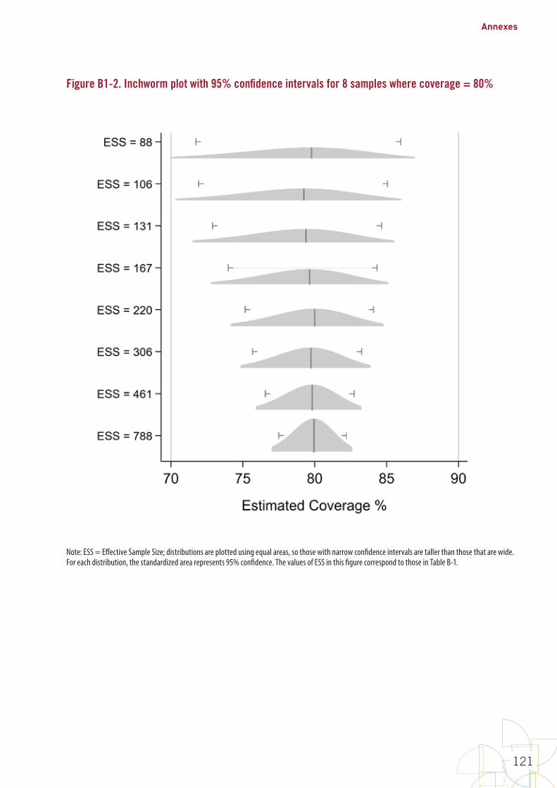
Annexes
121
Figure B1-2. Inchworm plot with 95% confidence intervals for 8 samples where coverage = 80%
Note: ESS = Effective Sample Size; distributions are plotted using equal areas, so those with narrow confidence intervals are taller than those that are wide. For each distribution, the standardized area represents 95% confidence. The values of ESS in this figure correspond to those in Table B-1.
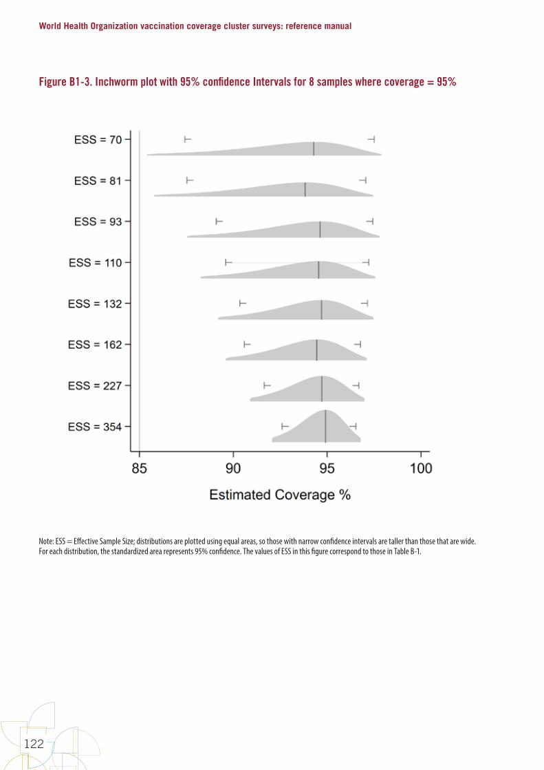
World Health Organization vaccination coverage cluster surveys: reference manual
122
Figure B1-3. Inchworm plot with 95% confidence Intervals for 8 samples where coverage = 95%
Note: ESS = Effective Sample Size; distributions are plotted using equal areas, so those with narrow confidence intervals are taller than those that are wide. For each distribution, the standardized area represents 95% confidence. The values of ESS in this figure correspond to those in Table B-1.

Annexes
123
Table B-2. Effective sample sizes (ESS) to classify coverage as being very likely BELOW a programmatic threshold
Programmatic Threshold (%) Delta (%)
alpha=10% power=80%
alpha=5% power=80%
alpha=10% power=90%
alpha=5% power=90%
ESS ESS ESS ESS50
1
11,368 15,555 16,521 21,506
55 11,273 15,421 16,389 21,330
60 10,953 14,978 15,929 20,725
65 10,407 14,226 15,141 19,692
70 9,636 13,165 14,024 18,230
75 8,640 11,795 12,579 16,341
80 7,418 10,115 10,804 14,023
85 5,970 8,126 8,701 11,276
90 4,296 5,827 6,269 8,100
95 2,396 3,217 3,506 4,494
50
5
469 637 674 873
55 468 635 674 872
60 458 620 661 854
65 439 593 634 818
70 411 554 595 766
75 374 502 542 696
80 328 438 476 609
85 272 362 397 504
90 208 272 304 382
95 133 169 196 241
50
10
121 163 171 221
55 122 163 173 222
60 120 161 171 220
65 116 155 166 213
70 110 146 158 201
75 102 134 146 186
80 91 119 131 165
85 78 101 113 141
90 62 79 91 111
95 44 53 64 77
50
15
55 74 77 98
55 56 74 78 100
60 56 74 78 100
65 54 72 77 97
70 52 68 74 93
75 49 63 69 87
80 44 57 63 79
85 38 49 55 68
90 32 40 46 56
95 24 28 35 41
World Health Organization vaccination coverage cluster surveys: reference manual
124
Note 1. Programmatic threshold is the expected coverage level.
Note 2. Delta is the difference (+ or –) from the programmatic threshold, from which you want to be well powered to reject the null hypothesis. For example, when ESS = 15,555, a classification based on an upper confidence limit will misclassify strata with true coverage of 50% only 5% of the time, and will have 80% power to correctly classify strata with true coverage of 49% or lower as having low coverage.
Note 3. This table conservatively provides ESS based on testing whether coverage is below a programmatic threshold (subtract delta from the programmatic threshold). In some cases, the ESS would be slightly smaller if testing whether coverage is above a programmatic threshold (adding delta to the programmatic threshold), as in Table B-3.
Note 4. For example, if the effective sample size is 146, from the column where alpha = 5%, and power = 80%, and programmatic threshold = 70%, and delta = 10%, then we might say the following: If true vaccination coverage is at least as low as (threshold – delta) = (70% – 10% = 60%) and we conduct numerous repeated surveys, each with an effective sample size of 146, when we calculate 100% –alpha% = (100% – 5% = 95%) upper confidence bound for all those surveys, we expect 80% of them to fall somewhere below 70%, leading to the correct and strong conclusion in at least 80% of those surveys, that we have 95% confidence that the population coverage is below 70%.
Of course, in practice we do not conduct many repeated surveys in a single stratum, and we do not know the true underlying population coverage figure, so we cannot know whether our classification is correct. Therefore, we power the survey to make it likely that the classifications will be correct, and we accept the risk that some classification outcomes will be incorrect due to sampling variability.
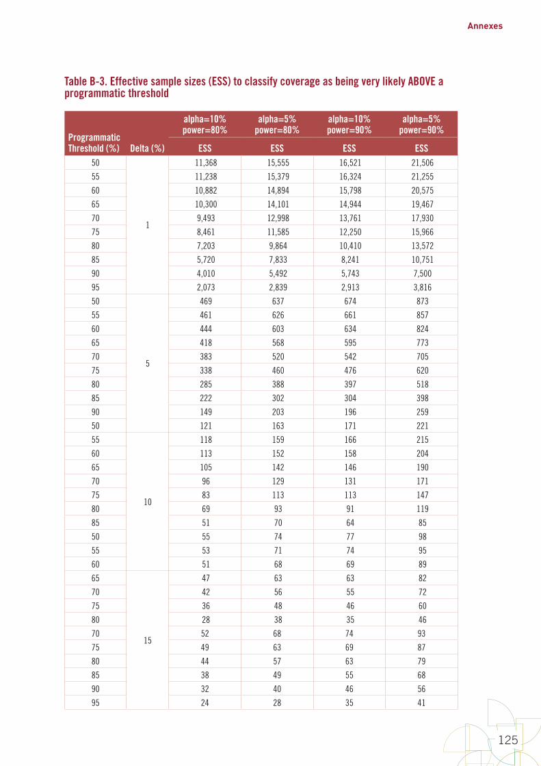
Annexes
125
Table B-3. Effective sample sizes (ESS) to classify coverage as being very likely ABOVE a programmatic threshold
Programmatic Threshold (%) Delta (%)
alpha=10% power=80%
alpha=5% power=80%
alpha=10% power=90%
alpha=5% power=90%
ESS ESS ESS ESS50
1
11,368 15,555 16,521 21,506
55 11,238 15,379 16,324 21,255
60 10,882 14,894 15,798 20,575
65 10,300 14,101 14,944 19,467
70 9,493 12,998 13,761 17,930
75 8,461 11,585 12,250 15,966
80 7,203 9,864 10,410 13,572
85 5,720 7,833 8,241 10,751
90 4,010 5,492 5,743 7,500
95 2,073 2,839 2,913 3,816
50
5
469 637 674 873
55 461 626 661 857
60 444 603 634 824
65 418 568 595 773
70 383 520 542 705
75 338 460 476 620
80 285 388 397 518
85 222 302 304 398
90 149 203 196 259
50 121 163 171 221
55
10
118 159 166 215
60 113 152 158 204
65 105 142 146 190
70 96 129 131 171
75 83 113 113 147
80 69 93 91 119
85 51 70 64 85
50 55 74 77 98
55 53 71 74 95
60 51 68 69 89
65
15
47 63 63 82
70 42 56 55 72
75 36 48 46 60
80 28 38 35 46
70 52 68 74 93
75 49 63 69 87
80 44 57 63 79
85 38 49 55 68
90 32 40 46 56
95 24 28 35 41
World Health Organization vaccination coverage cluster surveys: reference manual
126
Note 1. Programmatic threshold is the expected coverage level.
Note 2. Delta is the difference above the programmatic threshold (PT) from which you want to be well powered to reject the null hypothesis. For example, when ESS = 11,368, a classification based on a 1-sided upper (100-alpha) = (100–10) = 90% confidence limit will misclassify strata with true coverage >=50% no more than 10% of the time, and will have 80% power to correctly classify strata with true coverage of 51% or higher as having high coverage. In other words, if the true coverage is PT + Delta, then a survey of ESS will have at most alpha misclassification errors and at least 1 – beta power.
Note 3. This table provides ESS based on testing whether coverage is above a programmatic threshold (add delta to the programmatic threshold). In some cases, the ESS would be slightly larger if testing whether coverage is below a programmatic threshold (subtract delta from the programmatic threshold), as in Table B-2.
Note 4. For example, if the effective sample size is 129, from the column where alpha = 5%, and power = 80%, and the programmatic threshold = 70%, and delta = 10%, then we might say the following: If true vaccination coverage is at least threshold + delta (70% + 10% = 80%), and we conduct numerous repeated surveys that each have an effective sample size of 129, when we calculate the 100% – alpha% (100% – 5% = 95%) lower confidence bound for all those surveys, we expect 80% of them to fall somewhere above 70%. This leads to the correct and strong conclusion that in at least 80% of those surveys, population coverage is 95% likely to be higher than 70%.
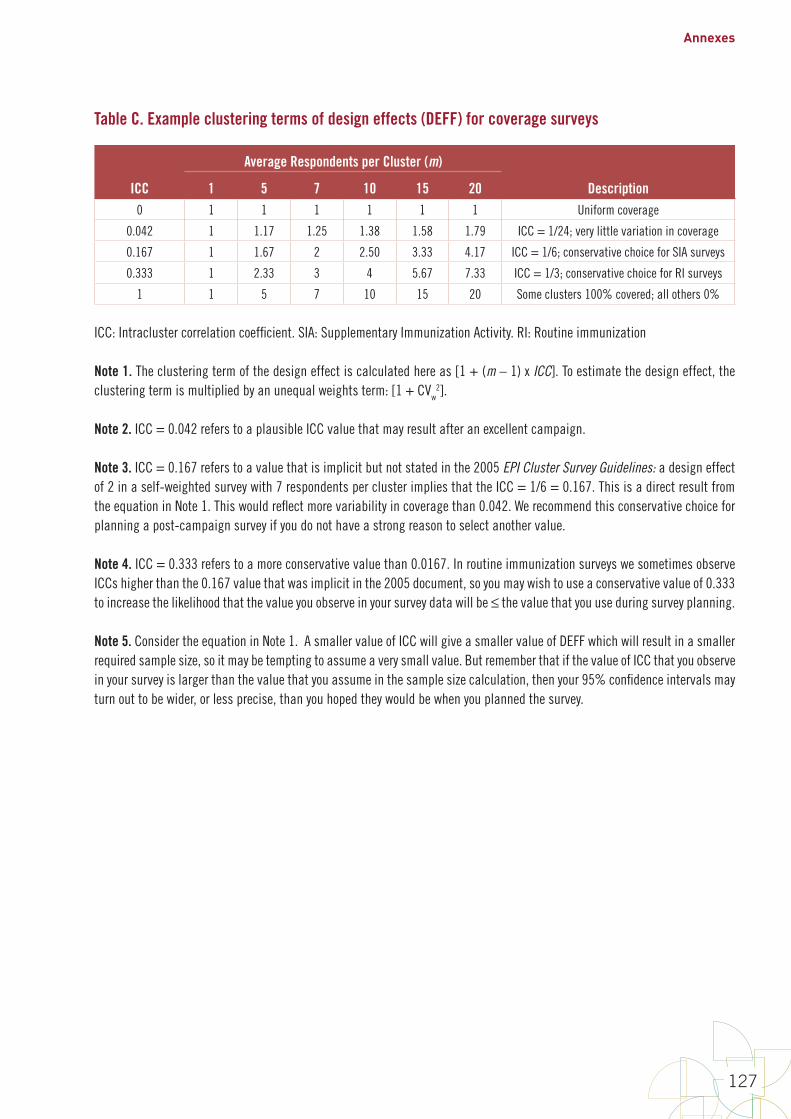
Annexes
127
Table C. Example clustering terms of design effects (DEFF) for coverage surveys
ICC
Average Respondents per Cluster (m)
Description1 5 7 10 15 200 1 1 1 1 1 1 Uniform coverage
0.042 1 1.17 1.25 1.38 1.58 1.79 ICC = 1/24; very little variation in coverage
0.167 1 1.67 2 2.50 3.33 4.17 ICC = 1/6; conservative choice for SIA surveys
0.333 1 2.33 3 4 5.67 7.33 ICC = 1/3; conservative choice for RI surveys
1 1 5 7 10 15 20 Some clusters 100% covered; all others 0%
ICC: Intracluster correlation coefficient. SIA: Supplementary Immunization Activity. RI: Routine immunization
Note 1. The clustering term of the design effect is calculated here as [1 + (m – 1) x ICC]. To estimate the design effect, the clustering term is multiplied by an unequal weights term: [1 + CVw
2].
Note 2. ICC = 0.042 refers to a plausible ICC value that may result after an excellent campaign.
Note 3. ICC = 0.167 refers to a value that is implicit but not stated in the 2005 EPI Cluster Survey Guidelines: a design effect of 2 in a self-weighted survey with 7 respondents per cluster implies that the ICC = 1/6 = 0.167. This is a direct result from the equation in Note 1. This would reflect more variability in coverage than 0.042. We recommend this conservative choice for planning a post-campaign survey if you do not have a strong reason to select another value.
Note 4. ICC = 0.333 refers to a more conservative value than 0.0167. In routine immunization surveys we sometimes observe ICCs higher than the 0.167 value that was implicit in the 2005 document, so you may wish to use a conservative value of 0.333 to increase the likelihood that the value you observe in your survey data will be ≤ the value that you use during survey planning.
Note 5. Consider the equation in Note 1. A smaller value of ICC will give a smaller value of DEFF which will result in a smaller required sample size, so it may be tempting to assume a very small value. But remember that if the value of ICC that you observe in your survey is larger than the value that you assume in the sample size calculation, then your 95% confidence intervals may turn out to be wider, or less precise, than you hoped they would be when you planned the survey.
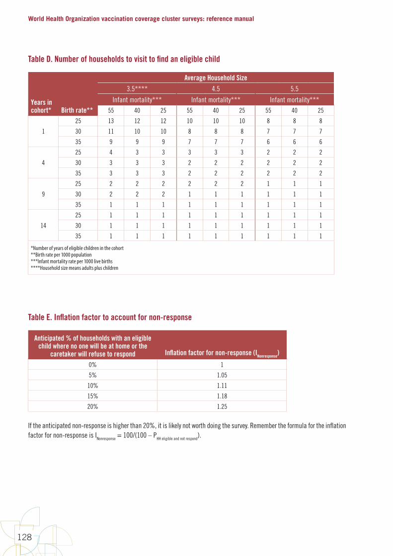
World Health Organization vaccination coverage cluster surveys: reference manual
128
Table D. Number of households to visit to find an eligible child
Years in cohort* Birth rate**
Average Household Size
3.5**** 4.5 5.5
Infant mortality*** Infant mortality*** Infant mortality***55 40 25 55 40 25 55 40 25
1
25 13 12 12 10 10 10 8 8 8
30 11 10 10 8 8 8 7 7 7
35 9 9 9 7 7 7 6 6 6
4
25 4 3 3 3 3 3 2 2 2
30 3 3 3 2 2 2 2 2 2
35 3 3 3 2 2 2 2 2 2
9
25 2 2 2 2 2 2 1 1 1
30 2 2 2 1 1 1 1 1 1
35 1 1 1 1 1 1 1 1 1
14
25 1 1 1 1 1 1 1 1 1
30 1 1 1 1 1 1 1 1 1
35 1 1 1 1 1 1 1 1 1
*Number of years of eligible children in the cohort**Birth rate per 1000 population***Infant mortality rate per 1000 live births****Household size means adults plus children
Table E. Inflation factor to account for non-response
Anticipated % of households with an eligible child where no one will be at home or the
caretaker will refuse to respond Inflation factor for non-response (INonresponse)
0% 1
5% 1.05
10% 1.11
15% 1.18
20% 1.25
If the anticipated non-response is higher than 20%, it is likely not worth doing the survey. Remember the formula for the inflation factor for non-response is INonresponse = 100/(100 – PHH eligible and not respond).
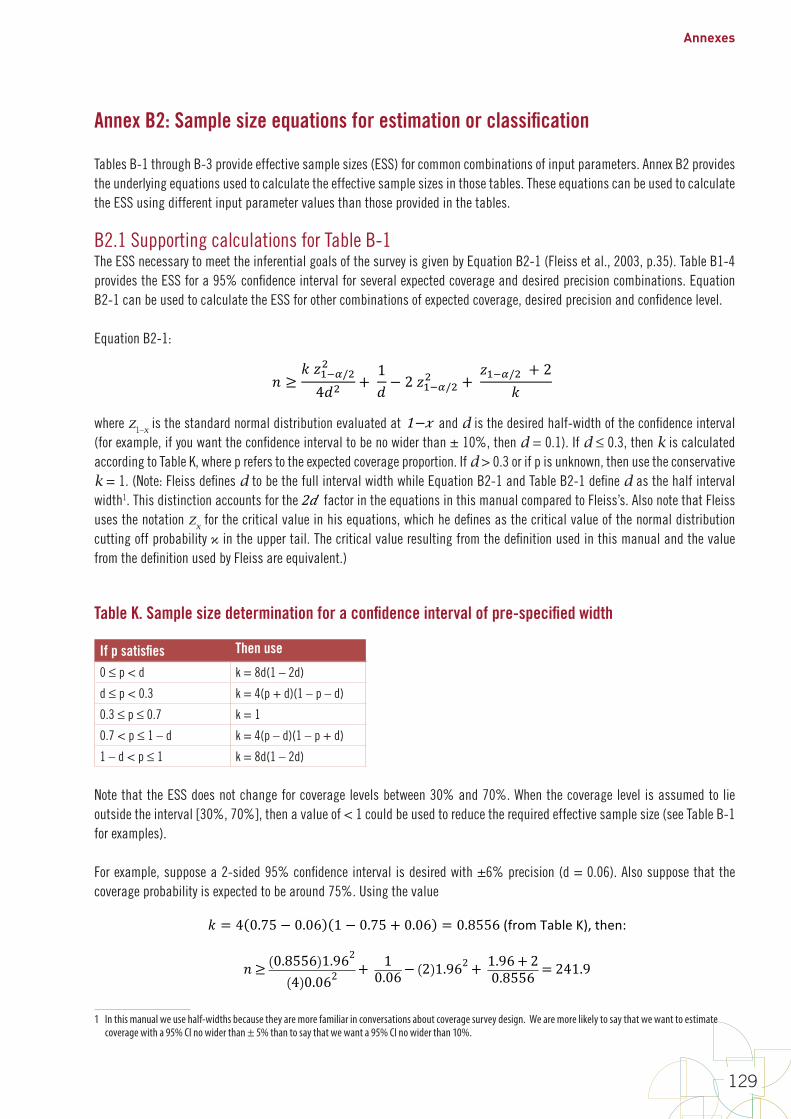
Annexes
129
Annex B2: Sample size equations for estimation or classification
Tables B-1 through B-3 provide effective sample sizes (ESS) for common combinations of input parameters. Annex B2 provides the underlying equations used to calculate the effective sample sizes in those tables. These equations can be used to calculate the ESS using different input parameter values than those provided in the tables.
B2.1 Supporting calculations for Table B-1The ESS necessary to meet the inferential goals of the survey is given by Equation B2-1 (Fleiss et al., 2003, p.35). Table B1-4 provides the ESS for a 95% confidence interval for several expected coverage and desired precision combinations. Equation B2-1 can be used to calculate the ESS for other combinations of expected coverage, desired precision and confidence level.
Equation B2-1:
B2-1
Annex B2: Sample size equations for estimation or classification TablesB-1throughB-3provideeffectivesamplesizes(ESS)forcommoncombinationsofinputparameters.AnnexB2providestheunderlyingequationsusedtocalculatetheeffectivesamplesizesinthosetables.TheseequationscanbeusedtocalculatetheESSusingdifferentinputparametervaluesthanthoseprovidedinthetables.
B2.1 Supporting calculations for Table B-1 TheESSnecessarytomeettheinferentialgoalsofthesurveyisgivenbyEquationB2-1(Fleissetal.,2003,p.35).TableB1-4providestheESSfora95%confidenceintervalforseveralexpectedcoverageanddesiredprecisioncombinations.EquationB2-1canbeusedtocalculatetheESSforothercombinationsofexpectedcoverage,desiredprecisionandconfidencelevel.
EquationB2-1:
) ≥*,-.//11
431 + 13 − 2,-.//11 + ,-.//1 + 2
*
where,-.5isthestandardnormaldistributionevaluatedat1–6and3isthedesiredhalf-widthoftheconfidenceinterval(forexample,ifyouwanttheconfidenceintervaltobenowiderthan±10%,thend=0.1).If3≤0.3,then*iscalculatedaccordingtoTableK,wherepreferstotheexpectedcoverageproportion.If3>0.3orifpisunknown,thenusetheconservative*=1.(Note:Fleissdefines3tobethefullintervalwidthwhileEquationB2-1andTableB2-1define3asthehalfintervalwidth2.Thisdistinctionaccountsforthe23factorintheequationsinthismanualcomparedtoFleiss’s.AlsonotethatFleissusesthenotation,5forthecriticalvalueinhisequations,whichhedefinesasthecriticalvalueofthenormaldistributioncuttingoffprobability6intheuppertail.ThecriticalvalueresultingfromthedefinitionusedinthismanualandthevaluefromthedefinitionusedbyFleissareequivalent.)
TableK.Samplesizedeterminationforaconfidenceintervalofpre-specifiedwidthIfpsatisfies Thenuse
0≤p<d k=8d(1–2d)d≤p<0.3 k=4(p+d)(1–p–d)0.3≤p≤0.7 k=10.7<p≤1–d k=4(p–d)(1–p+d)1–d<p≤1 k=8d(1–2d)
2Inthismanualweusehalf-widthsbecausetheyaremorefamiliarinconversationsaboutcoveragesurveydesign.Wearemorelikelytosaythatwewanttoestimatecoveragewitha95%CInowiderthan±5%thantosaythatwewanta95%CInowiderthan10%.
where z1–x is the standard normal distribution evaluated at
B2-‐1
Annex B2: Sample size equations for estimation or classification Tables B-‐1 through B-‐3 provide effective sample sizes (ESS) for common combinations of input parameters. Annex B2 provides the underlying equations used to calculate the effective sample sizes in those tables. These equations can be used to calculate the ESS using different input parameter values than those provided in the tables.
B2.1 Supporting calculations for Table B-1 The ESS necessary to meet the inferential goals of the survey is given by Equation B2-‐1 (Fleiss et al., 2003, p.35). Table B1-‐4 provides the ESS for a 95% confidence interval for several expected coverage and desired precision combinations. Equation B2-‐1 can be used to calculate the ESS for other combinations of expected coverage, desired precision and confidence level.
Equation B2-‐1:
𝑛𝑛≥𝑘𝑘 𝑧𝑧1−𝛼𝛼/224𝑑𝑑2+ 1𝑑𝑑−2 𝑧𝑧1−𝛼𝛼/22+ 𝑧𝑧1−𝛼𝛼/2 +2𝑘𝑘
where 𝑧𝑧1−𝑥𝑥 is the standard normal distribution evaluated at 1 – 𝑥𝑥 and 𝑑𝑑 is the desired half-‐width of the confidence interval (for example, if you want the confidence interval to be no wider than ± 10%, then d = 0.1). If 𝑑𝑑 ≤ 0.3, then 𝑘𝑘 is calculated according to Table K, where p refers to the expected coverage proportion. If 𝑑𝑑 > 0.3 or if p is unknown, then use the conservative 𝑘𝑘 = 1. (Note: Fleiss defines 𝑑𝑑 to be the full interval width while Equation B2-‐1 and Table B2-‐1 define 𝑑𝑑 as the half interval width2. This distinction accounts for the 2𝑑𝑑 factor in the equations in this manual compared to Fleiss’s. Also note that Fleiss uses the notation 𝑧𝑧𝑥𝑥 for the critical value in his equations, which he defines as the critical value of the normal distribution cutting off probability 𝑥𝑥 in the upper tail. The critical value resulting from the definition used in this manual and the value from the definition used by Fleiss are equivalent.)
Table K. Sample size determination for a confidence interval of pre-‐specified width If p satisfies Then use 0 ≤ p < d k = 8d(1 – 2d)
d ≤ p < 0.3 k = 4(p + d)(1 – p – d) 0.3 ≤ p ≤ 0.7 k = 1
0.7 < p ≤ 1 – d k = 4(p – d)(1 – p + d)
1 – d < p ≤ 1 k = 8d(1 – 2d)
2 In this manual we use half-‐widths because they are more familiar in conversations about coverage survey design. We are more likely to say that we want to estimate coverage with a 95% CI no wider than ± 5% than to say that we want a 95% CI no wider than 10%.
and d is the desired half-width of the confidence interval (for example, if you want the confidence interval to be no wider than ± 10%, then d = 0.1). If d ≤ 0.3, then k is calculated according to Table K, where p refers to the expected coverage proportion. If d > 0.3 or if p is unknown, then use the conservative k = 1. (Note: Fleiss defines d to be the full interval width while Equation B2-1 and Table B2-1 define d as the half interval width1. This distinction accounts for the
B2-‐1
Annex B2: Sample size equations for estimation or classification Tables B-‐1 through B-‐3 provide effective sample sizes (ESS) for common combinations of input parameters. Annex B2 provides the underlying equations used to calculate the effective sample sizes in those tables. These equations can be used to calculate the ESS using different input parameter values than those provided in the tables.
B2.1 Supporting calculations for Table B-1 The ESS necessary to meet the inferential goals of the survey is given by Equation B2-‐1 (Fleiss et al., 2003, p.35). Table B1-‐4 provides the ESS for a 95% confidence interval for several expected coverage and desired precision combinations. Equation B2-‐1 can be used to calculate the ESS for other combinations of expected coverage, desired precision and confidence level.
Equation B2-‐1:
𝑛𝑛≥𝑘𝑘 𝑧𝑧1−𝛼𝛼/224𝑑𝑑2+ 1𝑑𝑑−2 𝑧𝑧1−𝛼𝛼/22+ 𝑧𝑧1−𝛼𝛼/2 +2𝑘𝑘
where 𝑧𝑧1−𝑥𝑥 is the standard normal distribution evaluated at 1 – 𝑥𝑥 and 𝑑𝑑 is the desired half-‐width of the confidence interval (for example, if you want the confidence interval to be no wider than ± 10%, then d = 0.1). If 𝑑𝑑 ≤ 0.3, then 𝑘𝑘 is calculated according to Table K, where p refers to the expected coverage proportion. If 𝑑𝑑 > 0.3 or if p is unknown, then use the conservative 𝑘𝑘 = 1. (Note: Fleiss defines 𝑑𝑑 to be the full interval width while Equation B2-‐1 and Table B2-‐1 define 𝑑𝑑 as the half interval width2. This distinction accounts for the 2𝑑𝑑 factor in the equations in this manual compared to Fleiss’s. Also note that Fleiss uses the notation 𝑧𝑧𝑥𝑥 for the critical value in his equations, which he defines as the critical value of the normal distribution cutting off probability 𝑥𝑥 in the upper tail. The critical value resulting from the definition used in this manual and the value from the definition used by Fleiss are equivalent.)
Table K. Sample size determination for a confidence interval of pre-‐specified width If p satisfies Then use 0 ≤ p < d k = 8d(1 – 2d)
d ≤ p < 0.3 k = 4(p + d)(1 – p – d) 0.3 ≤ p ≤ 0.7 k = 1
0.7 < p ≤ 1 – d k = 4(p – d)(1 – p + d)
1 – d < p ≤ 1 k = 8d(1 – 2d)
2 In this manual we use half-‐widths because they are more familiar in conversations about coverage survey design. We are more likely to say that we want to estimate coverage with a 95% CI no wider than ± 5% than to say that we want a 95% CI no wider than 10%.
factor in the equations in this manual compared to Fleiss’s. Also note that Fleiss uses the notation z
x for the critical value in his equations, which he defines as the critical value of the normal distribution
cutting off probability in the upper tail. The critical value resulting from the definition used in this manual and the value from the definition used by Fleiss are equivalent.)
Table K. Sample size determination for a confidence interval of pre-specified width
If p satisfies Then use
0 ≤ p < d k = 8d(1 – 2d)
d ≤ p < 0.3 k = 4(p + d)(1 – p – d)
0.3 ≤ p ≤ 0.7 k = 1
0.7 < p ≤ 1 – d k = 4(p – d)(1 – p + d)
1 – d < p ≤ 1 k = 8d(1 – 2d)
Note that the ESS does not change for coverage levels between 30% and 70%. When the coverage level is assumed to lie outside the interval [30%, 70%], then a value of < 1 could be used to reduce the required effective sample size (see Table B-1 for examples).
For example, suppose a 2-sided 95% confidence interval is desired with ±6% precision (d = 0.06). Also suppose that the coverage probability is expected to be around 75%. Using the value
B2-2
NotethattheESSdoesnotchangeforcoveragelevelsbetween30%and70%.Whenthecoveragelevelisassumedtolieoutsidetheinterval[30%,70%],thenavalueof*<1couldbeusedtoreducetherequiredeffectivesamplesize(seeTableB-1forexamples).
Forexample,supposea2-sided95%confidenceintervalisdesiredwith±6%precision(d=0.06).Alsosupposethatthecoverageprobabilityisexpectedtobearound75%.Usingthevalue
* = 4 0.75 − 0.06 1 − 0.75 + 0.06 = 0.8556(fromTableK),then:
) ≥ 0.8556 1.962
4 0.062+ 1
0.06− 2 1.962 +1.96+ 20.8556 = 241.9
Rounduptothenearestchildwholenumber,sothattheESSis)≥242.WiththisESS,ifasimplerandomsampleweretaken,thena95%confidenceintervalwillbeatmost±6%foranyobservedcoveragevalueofcoverage75%orhigher.
B2.2 Supporting calculations for Tables B-2 and B-3 Ifsufficientresourcesarenotavailabletoobtainverypreciseresultsineverystratum,itcanbehelpfultoselectasamplesizebasedonthepowertousea1-sidedhypothesistesttoclassifycoverageinthosestrataasbeinghigherorlowerthanafixedprogrammaticthreshold.Coveragewilleitherbe:
• verylikelylowerthantheprogrammaticthreshold• verylikelyhigherthanthethreshold,or• notdistinguishablefromthethresholdwithhighconfidence,usingthesamplesizeinthissurvey.
ThisdesignrequiresfiveinputparameterstobespecifiedinordertocalculatethecorrespondingESS.Theyaredefinedasfollows:
1. Theprogrammaticthreshold(PTor?@)isacoveragelevelofinterest,suchasmightbethecoveragetargetortheexpectedcoveragelevel.
2. Deltaisacoveragepercentdefiningadistancefromtheprogrammaticthreshold.Ifthetruecoverageisatleastdeltapointsawayfromtheprogrammaticthreshold,thenwepickasamplesizelikelytoclassifythosedistrictsashavingcoveragelikelydifferentthandelta.Forexample,iftheprogrammaticthresholdis80%anddeltais5%,thenwhencoverageis80–5=75%(orlower)or80+5=85%(orhigher),youwantthesurveyresultstobeverylikelytoshowthatcoverageisverylikelylowerorhigherthan80%,respectively.
3. Directionindicateswhetheryouarespecifyingstatisticalpowerforcorrectlyclassifyingstratawithcoveragedeltapercentabovetheprogrammaticthreshold,ordeltapercentbelowtheprogrammaticthreshold.Ifthethresholdofinterestis80%andyouwanttobeverysuretocorrectlyclassifystratawith90%orgreatercoverage,thenthedirectionisaboveandyoushoulduseTableB-3tolookuptheESS.IfthedirectionisbelowthenuseTableB-2.NotethattheeffectivesamplesizesinB-2arelargerthanthoseinB1-6,sotheconservativechoiceistouseTableB-2unlessyouareveryfocusedondetectingdifferencesabovetheprogrammaticthreshold.
1 In this manual we use half-widths because they are more familiar in conversations about coverage survey design. We are more likely to say that we want to estimate coverage with a 95% CI no wider than ± 5% than to say that we want a 95% CI no wider than 10%.
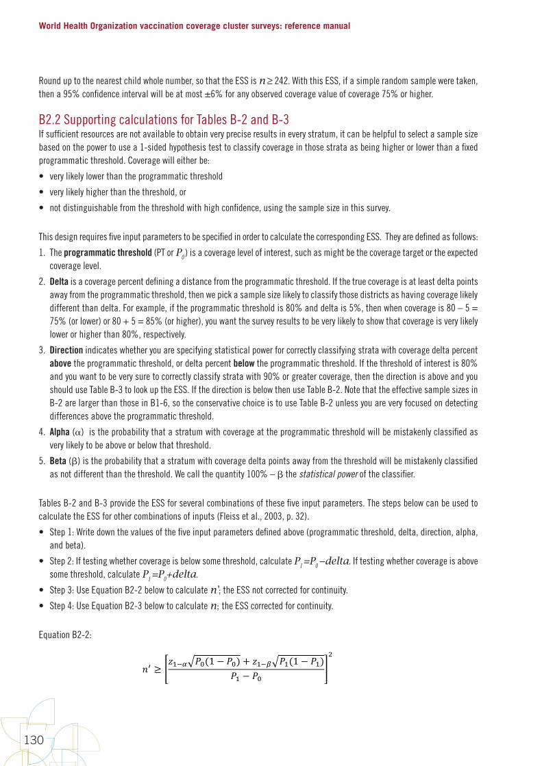
World Health Organization vaccination coverage cluster surveys: reference manual
130
Round up to the nearest child whole number, so that the ESS is n ≥ 242. With this ESS, if a simple random sample were taken, then a 95% confidence interval will be at most ±6% for any observed coverage value of coverage 75% or higher.
B2.2 Supporting calculations for Tables B-2 and B-3If sufficient resources are not available to obtain very precise results in every stratum, it can be helpful to select a sample size based on the power to use a 1-sided hypothesis test to classify coverage in those strata as being higher or lower than a fixed programmatic threshold. Coverage will either be:
• very likely lower than the programmatic threshold
• very likely higher than the threshold, or
• not distinguishable from the threshold with high confidence, using the sample size in this survey.
This design requires five input parameters to be specified in order to calculate the corresponding ESS. They are defined as follows:
1. The programmatic threshold (PT or P0 ) is a coverage level of interest, such as might be the coverage target or the expected coverage level.
2. Delta is a coverage percent defining a distance from the programmatic threshold. If the true coverage is at least delta points away from the programmatic threshold, then we pick a sample size likely to classify those districts as having coverage likely different than delta. For example, if the programmatic threshold is 80% and delta is 5%, then when coverage is 80 – 5 = 75% (or lower) or 80 + 5 = 85% (or higher), you want the survey results to be very likely to show that coverage is very likely lower or higher than 80%, respectively.
3. Direction indicates whether you are specifying statistical power for correctly classifying strata with coverage delta percent above the programmatic threshold, or delta percent below the programmatic threshold. If the threshold of interest is 80% and you want to be very sure to correctly classify strata with 90% or greater coverage, then the direction is above and you should use Table B-3 to look up the ESS. If the direction is below then use Table B-2. Note that the effective sample sizes in B-2 are larger than those in B1-6, so the conservative choice is to use Table B-2 unless you are very focused on detecting differences above the programmatic threshold.
4. Alpha () is the probability that a stratum with coverage at the programmatic threshold will be mistakenly classified as very likely to be above or below that threshold.
5. Beta () is the probability that a stratum with coverage delta points away from the threshold will be mistakenly classified as not different than the threshold. We call the quantity 100% – the statistical power of the classifier.
Tables B-2 and B-3 provide the ESS for several combinations of these five input parameters. The steps below can be used to calculate the ESS for other combinations of inputs (Fleiss et al., 2003, p. 32).
• Step 1: Write down the values of the five input parameters defined above (programmatic threshold, delta, direction, alpha, and beta).
• Step 2: If testing whether coverage is below some threshold, calculate P1 =P0 −delta. If testing whether coverage is above some threshold, calculate P1 =P0+delta.
• Step 3: Use Equation B2-2 below to calculate n'; the ESS not corrected for continuity.
• Step 4: Use Equation B2-3 below to calculate n; the ESS corrected for continuity.
Equation B2-2:
B2-3
4. Alpha(α)istheprobabilitythatastratumwithcoverageattheprogrammaticthresholdwillbemistakenlyclassifiedasverylikelytobeaboveorbelowthatthreshold.
5. Beta(β)istheprobabilitythatastratumwithcoveragedeltapointsawayfromthethresholdwillbemistakenlyclassifiedasnotdifferentthanthethreshold.Wecallthequantity100%–βthestatisticalpoweroftheclassifier.
TablesB-2andB-3providetheESSforseveralcombinationsofthesefiveinputparameters.ThestepsbelowcanbeusedtocalculatetheESSforothercombinationsofinputs(Fleissetal.,2003,p.32).
• Step1:Writedownthevaluesofthefiveinputparametersdefinedabove(programmaticthreshold,delta,direction,alpha,andbeta).
• Step2:Iftestingwhethercoverageisbelowsomethreshold,calculate?- = ?@ − 3ABCD.Iftestingwhethercoverageisabovesomethreshold,calculate?- = ?@ + 3ABC.
• Step3:UseEquationB2-2belowtocalculate)E;theESSnotcorrectedforcontinuity.• Step4:UseEquationB2-3belowtocalculate);theESScorrectedforcontinuity.
EquationB2-2:
)E ≥,-./ ?@(1 − ?@) + ,-.H ?-(1 − ?-)
?- − ?@
1
where,-.5isthestandardnormaldistributionevaluatedat1–x.
EquationB2-3:
) ≥ )E4 1 + 1 + 2
)E ?- − ?@
1
Forexample,supposethecoveragetargetlevelis85%(thatis,PT=0.85),delta=10%,α=5%,andβ=20%(power=100%–20%=80%).Ifitisdesiredtoclassifycoverageasbeingverylikelybelowtheprogrammaticthreshold,(directionisbelow),thenwecalculate?-=0.85–0.10=0.75andfind
)E ≥ 1.645 0.85 1 − 0.85 + 0.842 0.75 1 − 0.750.75 − 0.85
1
= 90.6
Round)EuptothenearestchildwholenumberandsubstituteitintoEquationB2-3toget
) ≥ 914 1 + 1 + 2
91 0.75 − 0.85
1
= 100.8
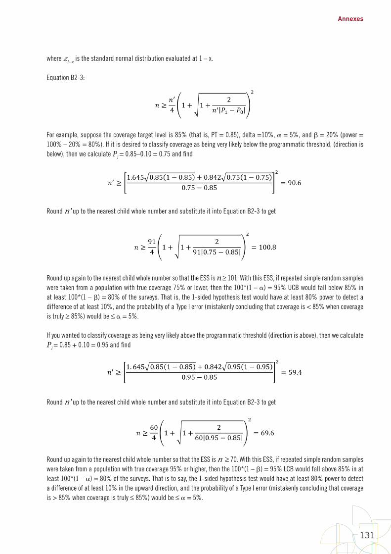
Annexes
131
where z1− is the standard normal distribution evaluated at 1 – x.
Equation B2-3:
B2-3
4. Alpha(α)istheprobabilitythatastratumwithcoverageattheprogrammaticthresholdwillbemistakenlyclassifiedasverylikelytobeaboveorbelowthatthreshold.
5. Beta(β)istheprobabilitythatastratumwithcoveragedeltapointsawayfromthethresholdwillbemistakenlyclassifiedasnotdifferentthanthethreshold.Wecallthequantity100%–βthestatisticalpoweroftheclassifier.
TablesB-2andB-3providetheESSforseveralcombinationsofthesefiveinputparameters.ThestepsbelowcanbeusedtocalculatetheESSforothercombinationsofinputs(Fleissetal.,2003,p.32).
• Step1:Writedownthevaluesofthefiveinputparametersdefinedabove(programmaticthreshold,delta,direction,alpha,andbeta).
• Step2:Iftestingwhethercoverageisbelowsomethreshold,calculate?- = ?@ − 3ABCD.Iftestingwhethercoverageisabovesomethreshold,calculate?- = ?@ + 3ABC.
• Step3:UseEquationB2-2belowtocalculate)E;theESSnotcorrectedforcontinuity.• Step4:UseEquationB2-3belowtocalculate);theESScorrectedforcontinuity.
EquationB2-2:
)E ≥,-./ ?@(1 − ?@) + ,-.H ?-(1 − ?-)
?- − ?@
1
where,-.5isthestandardnormaldistributionevaluatedat1–x.
EquationB2-3:
) ≥ )E4 1 + 1 + 2
)E ?- − ?@
1
Forexample,supposethecoveragetargetlevelis85%(thatis,PT=0.85),delta=10%,α=5%,andβ=20%(power=100%–20%=80%).Ifitisdesiredtoclassifycoverageasbeingverylikelybelowtheprogrammaticthreshold,(directionisbelow),thenwecalculate?-=0.85–0.10=0.75andfind
)E ≥ 1.645 0.85 1 − 0.85 + 0.842 0.75 1 − 0.750.75 − 0.85
1
= 90.6
Round)EuptothenearestchildwholenumberandsubstituteitintoEquationB2-3toget
) ≥ 914 1 + 1 + 2
91 0.75 − 0.85
1
= 100.8
For example, suppose the coverage target level is 85% (that is, PT = 0.85), delta =10%, = 5%, and = 20% (power = 100% – 20% = 80%). If it is desired to classify coverage as being very likely below the programmatic threshold, (direction is below), then we calculate P1 = 0.85–0.10 = 0.75 and find
B2-3
4. Alpha(α)istheprobabilitythatastratumwithcoverageattheprogrammaticthresholdwillbemistakenlyclassifiedasverylikelytobeaboveorbelowthatthreshold.
5. Beta(β)istheprobabilitythatastratumwithcoveragedeltapointsawayfromthethresholdwillbemistakenlyclassifiedasnotdifferentthanthethreshold.Wecallthequantity100%–βthestatisticalpoweroftheclassifier.
TablesB-2andB-3providetheESSforseveralcombinationsofthesefiveinputparameters.ThestepsbelowcanbeusedtocalculatetheESSforothercombinationsofinputs(Fleissetal.,2003,p.32).
• Step1:Writedownthevaluesofthefiveinputparametersdefinedabove(programmaticthreshold,delta,direction,alpha,andbeta).
• Step2:Iftestingwhethercoverageisbelowsomethreshold,calculate?- = ?@ − 3ABCD.Iftestingwhethercoverageisabovesomethreshold,calculate?- = ?@ + 3ABC.
• Step3:UseEquationB2-2belowtocalculate)E;theESSnotcorrectedforcontinuity.• Step4:UseEquationB2-3belowtocalculate);theESScorrectedforcontinuity.
EquationB2-2:
)E ≥,-./ ?@(1 − ?@) + ,-.H ?-(1 − ?-)
?- − ?@
1
where,-.5isthestandardnormaldistributionevaluatedat1–x.
EquationB2-3:
) ≥ )E4 1 + 1 + 2
)E ?- − ?@
1
Forexample,supposethecoveragetargetlevelis85%(thatis,PT=0.85),delta=10%,α=5%,andβ=20%(power=100%–20%=80%).Ifitisdesiredtoclassifycoverageasbeingverylikelybelowtheprogrammaticthreshold,(directionisbelow),thenwecalculate?-=0.85–0.10=0.75andfind
)E ≥ 1.645 0.85 1 − 0.85 + 0.842 0.75 1 − 0.750.75 − 0.85
1
= 90.6
Round)EuptothenearestchildwholenumberandsubstituteitintoEquationB2-3toget
) ≥ 914 1 + 1 + 2
91 0.75 − 0.85
1
= 100.8
Round n' up to the nearest child whole number and substitute it into Equation B2-3 to get
B2-3
4. Alpha(α)istheprobabilitythatastratumwithcoverageattheprogrammaticthresholdwillbemistakenlyclassifiedasverylikelytobeaboveorbelowthatthreshold.
5. Beta(β)istheprobabilitythatastratumwithcoveragedeltapointsawayfromthethresholdwillbemistakenlyclassifiedasnotdifferentthanthethreshold.Wecallthequantity100%–βthestatisticalpoweroftheclassifier.
TablesB-2andB-3providetheESSforseveralcombinationsofthesefiveinputparameters.ThestepsbelowcanbeusedtocalculatetheESSforothercombinationsofinputs(Fleissetal.,2003,p.32).
• Step1:Writedownthevaluesofthefiveinputparametersdefinedabove(programmaticthreshold,delta,direction,alpha,andbeta).
• Step2:Iftestingwhethercoverageisbelowsomethreshold,calculate?- = ?@ − 3ABCD.Iftestingwhethercoverageisabovesomethreshold,calculate?- = ?@ + 3ABC.
• Step3:UseEquationB2-2belowtocalculate)E;theESSnotcorrectedforcontinuity.• Step4:UseEquationB2-3belowtocalculate);theESScorrectedforcontinuity.
EquationB2-2:
)E ≥,-./ ?@(1 − ?@) + ,-.H ?-(1 − ?-)
?- − ?@
1
where,-.5isthestandardnormaldistributionevaluatedat1–x.
EquationB2-3:
) ≥ )E4 1 + 1 + 2
)E ?- − ?@
1
Forexample,supposethecoveragetargetlevelis85%(thatis,PT=0.85),delta=10%,α=5%,andβ=20%(power=100%–20%=80%).Ifitisdesiredtoclassifycoverageasbeingverylikelybelowtheprogrammaticthreshold,(directionisbelow),thenwecalculate?-=0.85–0.10=0.75andfind
)E ≥ 1.645 0.85 1 − 0.85 + 0.842 0.75 1 − 0.750.75 − 0.85
1
= 90.6
Round)EuptothenearestchildwholenumberandsubstituteitintoEquationB2-3toget
) ≥ 914 1 + 1 + 2
91 0.75 − 0.85
1
= 100.8
Round up again to the nearest child whole number so that the ESS is n ≥ 101. With this ESS, if repeated simple random samples were taken from a population with true coverage 75% or lower, then the 100*(1 – ) = 95% UCB would fall below 85% in at least 100*(1 – ) = 80% of the surveys. That is, the 1-sided hypothesis test would have at least 80% power to detect a difference of at least 10%, and the probability of a Type I error (mistakenly concluding that coverage is < 85% when coverage is truly ≥ 85%) would be ≤ = 5%.
If you wanted to classify coverage as being very likely above the programmatic threshold (direction is above), then we calculate P1 = 0.85 + 0.10 = 0.95 and find
B2-4
RoundupagaintothenearestchildwholenumbersothattheESSis)≥101.WiththisESS,ifrepeatedsimplerandomsamplesweretakenfromapopulationwithtruecoverage75%orlower,thenthe100*(1–α)=95%UCBwouldfallbelow85%inatleast100*(1–β)=80%ofthesurveys.Thatis,the1-sidedhypothesistestwouldhaveatleast80%powertodetectadifferenceofatleast10%,andtheprobabilityofaTypeIerror(mistakenlyconcludingthatcoverageis<85%whencoverageistruly≥85%)wouldbe≤α=5%.
Ifyouwantedtoclassifycoverageasbeingverylikelyabovetheprogrammaticthreshold(directionisabove),thenwecalculate?-=0.85+0.10=0.95andfind
)E ≥ 1. 645 0.85 1 − 0.85 + 0.842 0.95 1 − 0.950.95 − 0.85
1
= 59.4
Round)EuptothenearestchildwholenumberandsubstituteitintoEquationB2-3toget
) ≥ 604 1 + 1 + 2
60 0.95 − 0.85
1
= 69.6
RoundupagaintothenearestchildwholenumbersothattheESSis)≥70.WiththisESS,ifrepeatedsimplerandomsamplesweretakenfromapopulationwithtruecoverage95%orhigher,thenthe100*(1–α)=95%LCBwouldfallabove85%inatleast100*(1–β)=80%ofthesurveys.Thatistosay,the1-sidedhypothesistestwouldhaveatleast80%powertodetectadifferenceofatleast10%intheupwarddirection,andtheprobabilityofaTypeIerror(mistakenlyconcludingthatcoverageis>85%whencoverageistruly≤85%)wouldbe≤α=5%.
Round n' up to the nearest child whole number and substitute it into Equation B2-3 to get
B2-4
RoundupagaintothenearestchildwholenumbersothattheESSis)≥101.WiththisESS,ifrepeatedsimplerandomsamplesweretakenfromapopulationwithtruecoverage75%orlower,thenthe100*(1–α)=95%UCBwouldfallbelow85%inatleast100*(1–β)=80%ofthesurveys.Thatis,the1-sidedhypothesistestwouldhaveatleast80%powertodetectadifferenceofatleast10%,andtheprobabilityofaTypeIerror(mistakenlyconcludingthatcoverageis<85%whencoverageistruly≥85%)wouldbe≤α=5%.
Ifyouwantedtoclassifycoverageasbeingverylikelyabovetheprogrammaticthreshold(directionisabove),thenwecalculate?-=0.85+0.10=0.95andfind
)E ≥ 1. 645 0.85 1 − 0.85 + 0.842 0.95 1 − 0.950.95 − 0.85
1
= 59.4
Round)EuptothenearestchildwholenumberandsubstituteitintoEquationB2-3toget
) ≥ 604 1 + 1 + 2
60 0.95 − 0.85
1
= 69.6
RoundupagaintothenearestchildwholenumbersothattheESSis)≥70.WiththisESS,ifrepeatedsimplerandomsamplesweretakenfromapopulationwithtruecoverage95%orhigher,thenthe100*(1–α)=95%LCBwouldfallabove85%inatleast100*(1–β)=80%ofthesurveys.Thatistosay,the1-sidedhypothesistestwouldhaveatleast80%powertodetectadifferenceofatleast10%intheupwarddirection,andtheprobabilityofaTypeIerror(mistakenlyconcludingthatcoverageis>85%whencoverageistruly≤85%)wouldbe≤α=5%.
Round up again to the nearest child whole number so that the ESS is n ≥ 70. With this ESS, if repeated simple random samples were taken from a population with true coverage 95% or higher, then the 100*(1 – ) = 95% LCB would fall above 85% in at least 100*(1 – ) = 80% of the surveys. That is to say, the 1-sided hypothesis test would have at least 80% power to detect a difference of at least 10% in the upward direction, and the probability of a Type I error (mistakenly concluding that coverage is > 85% when coverage is truly ≤ 85%) would be ≤ = 5%.

World Health Organization vaccination coverage cluster surveys: reference manual
132
Annex B3: Sample size equations for comparisons between places or subgroups, or over time
Annexes B1 and B2 were concerned with designing a single survey to meet an inferential goal. Annex B3 explains how to calculate the sample size for a survey that will conduct comparisons, either (1) between subgroups in a single survey (such as urban and rural), (2) between two simultaneous surveys (one survey in each place, Province A and Province B), or (3) between results of two surveys conducted at different time points (that is, changes over time). Comparing results over time could either mean two future surveys (to be conducted at different time points) or a past survey and a future survey. Of the three types of comparison, the first two are the most straightforward.
Regardless of the type of comparison, in order to make a meaningful comparison between surveys, many things about the two surveys should be the same:
• Both surveys should use probability samples selected in the same manner, using the same eligibility criteria.
• Both should use similar methods of fieldwork and similar questionnaires and training. Both should have roughly similar proportions of respondents who give evidence of vaccination by card and by caretaker recall.
In other words, the sources of non-sampling bias or error must be very nearly similar in order to attribute observed differences to actual improvements in vaccination coverage. We do not recommend conducting a new, large, and expensive survey for which the primary inferential goal is to measure change comparing with an earlier survey, if there are questions about the older survey’s details of the implementation or the quality of the work.
If you are planning two surveys simultaneously among different subgroups, and can control the quality and implementation of both, then sources of non-sampling bias or error are likely to be very similar in both surveys. There may be differences in ICC between the two subgroups, and there may be differences in sample sizes; both are accounted for in the guidelines presented here.
Looking for differences in coverage over time works best when you are planning two future surveys, one now and another in several years, so you can control the quality and implementation of both surveys. In that context, it may be possible to make meaningful comparisons between surveys over time. The guidelines presented here can help plan for those situations. The comparison is trickier when the earlier survey occurred in the past and you wish to do a new survey to show that coverage has improved. Some aspects that affect the quality of the earlier survey may be undocumented and difficult to learn. Many aspects of the two surveys may differ, so it will be challenging to draw a strong conclusion that observed differences in coverage are due to underlying differences in population coverage, and not due to other differences in survey design and implementation.
The methods for calculating the sample sizes necessary to conduct comparisons between two future surveys (to be conducted at different time points) are similar to the methods for calculating the sample sizes necessary to compare results between subgroups in a single survey or in two simultaneous surveys (one survey in each place). The next section of this annex discusses these methods. The methods for calculating sample sizes required to compare a past survey and a future survey are discussed near the end of this annex.

Annexes
133
B3.1 Testing for differences in vaccination coverage between places or subgroups, or between two future surveys In this section, we use the term between places, which may be interpreted to mean between groups or between two surveys in the future.
Table B-4 lists effective sample sizes for conducting two surveys of identical size for the purpose of detecting a statistically significant difference in estimated coverage between the two places. The effective sample sizes listed in the table are for each survey. The sample sizes are for a 2-sided test, where the null hypothesis is that coverage is the same in the two places, and the alternative hypothesis is that coverage differs. As with earlier comparisons, alpha is the probability of making a Type I error, or mistakenly concluding that there is a significant difference in coverage. Beta is the probability of making a Type II error, or mistakenly concluding there is no difference when in fact the population coverage difference between the two places is at least delta. Delta is the amount of difference for which you hope to power the comparison, and P1 is the value of coverage that is lower, if there is any difference.
For example, if you conducted surveys in Provinces A and B, each of which had effective sample sizes of 1,291 respondents, and expected coverage in one province was 70%, then you would have 80% power to detect a statistically significant difference using a 2-sided test, if the true prevalence was 75% or higher in the other province. The probability of making a Type I error, and mistakenly detecting a difference would be no more than alpha, or 5%.
The equations described in the text after Table B-4 give guidance on calculating sample sizes for parameters not covered in the table, or for unequal sample sizes in the two places. Those equations help calculate the effective sample size (ESS) needed to power the hypothesis test adequately. Use the equations listed in this section to calculate an ESS that will do the job, and then refer back to Annex B1 of the annex to calculate items C (the design effect), D (the number of households needed to find an eligible candidate), and E (the inflation factor for non-response). At that point you can substitute the ESS from this section in for factor B, and proceed with the calculations listed under Step 6 in Annex B1.
Note that these equations are for conducting a 2-sided test. If two future surveys are to be conducted at different points z1−
in Equation B2-1. This will potentially result in smaller effective sample sizes.
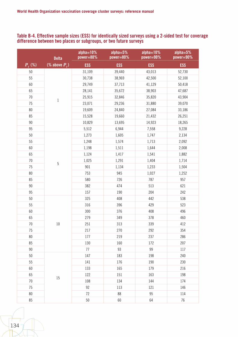
World Health Organization vaccination coverage cluster surveys: reference manual
134
Table B-4. Effective sample sizes (ESS) for identically sized surveys using a 2-sided test for coverage difference between two places or subgroups, or two future surveys
P1 (%)Delta
(% above P1 )
alpha=10% power=80%
alpha=5% power=80%
alpha=10% power=90%
alpha=5% power=90%
ESS ESS ESS ESS50
1
31,109 39,440 43,013 52,730
55 30,738 38,969 42,500 52,100
60 29,749 37,713 41,129 50,418
65 28,141 35,672 38,903 47,687
70 25,915 32,846 35,820 43,904
75 23,071 29,236 31,880 39,070
80 19,609 24,840 27,084 33,186
85 15,528 19,660 21,432 26,251
90 10,829 13,695 14,923 18,265
95 5,512 6,944 7,558 9,228
50
5
1,273 1,605 1,747 2,134
55 1,248 1,574 1,713 2,092
60 1,198 1,511 1,644 2,008
65 1,124 1,417 1,541 1,882
70 1,025 1,291 1,404 1,714
75 901 1,134 1,233 1,504
80 753 945 1,027 1,252
85 580 726 787 957
90 382 474 513 621
95 157 190 204 242
50
10
325 408 442 538
55 316 396 429 523
60 300 376 408 496
65 279 349 378 460
70 251 313 339 412
75 217 270 292 354
80 177 219 237 286
85 130 160 172 207
90 77 93 99 117
50
15
147 183 198 240
55 141 176 190 230
60 133 165 179 216
65 122 151 163 198
70 108 134 144 174
75 92 113 121 146
80 72 88 95 114
85 50 60 64 76
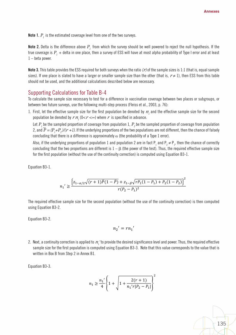
Annexes
135
Note 1. P1 is the estimated coverage level from one of the two surveys.
Note 2. Delta is the difference above P1 from which the survey should be well powered to reject the null hypothesis. If the true coverage is P1 + delta in one place, then a survey of ESS will have at most alpha probability of Type I error and at least 1 – beta power.
Note 3. This table provides the ESS required for both surveys when the ratio (r) of the sample sizes is 1:1 (that is, equal sample sizes). If one place is slated to have a larger or smaller sample size than the other (that is, r ≠ 1), then ESS from this table should not be used, and the additional calculations described below are necessary.
Supporting Calculations for Table B-4To calculate the sample size necessary to test for a difference in vaccination coverage between two places or subgroups, or between two future surveys, use the following multi-step process (Fleiss et al., 2003, p. 76):
1. First, let the effective sample size for the first population be denoted by n1 and the effective sample size for the second population be denoted by r n1 (0<r <∞) where r is specified in advance.
Let P1 be the sampled proportion of coverage from population 1, P2 be the sampled proportion of coverage from population 2, and P = (P1+P2 )/(r +1). If the underlying proportions of the two populations are not different, then the chance of falsely concluding that there is a difference is approximately (the probability of a Type 1 error).
Also, if the underlying proportions of population 1 and population 2 are in fact P1 and P2 ≠ P1, then the chance of correctly concluding that the two proportions are different is 1 – (the power of the test). Thus, the required effective sample size for the first population (without the use of the continuity correction) is computed using Equation B3-1.
Equation B3-1.
B3-4
Note1.P1istheestimatedcoveragelevelfromoneofthetwosurveys.
Note2.DeltaisthedifferenceaboveP1fromwhichthesurveyshouldbewellpoweredtorejectthenullhypothesis.IfthetruecoverageisP1+deltainoneplace,thenasurveyofESSwillhaveatmostalphaprobabilityofTypeIerrorandatleast1–betapower.
Note3.ThistableprovidestheESSrequiredforbothsurveyswhentheratio(r)ofthesamplesizesis1:1(thatis,equalsamplesizes).Ifoneplaceisslatedtohavealargerorsmallersamplesizethantheother(thatis,r≠1),thenESSfromthistableshouldnotbeused,andtheadditionalcalculationsdescribedbelowarenecessary.
Supporting Calculations for Table B-4 Tocalculatethesamplesizenecessarytotestforadifferenceinvaccinationcoveragebetweentwoplacesorsubgroups,orbetweentwofuturesurveys,usethefollowingmulti-stepprocess(Fleissetal.,2003,p.76):
1. First,lettheeffectivesamplesizeforthefirstpopulationbedenotedby)-andtheeffectivesamplesizeforthesecondpopulationbedenotedbyI)-(0 < I < ∞)whereIisspecifiedinadvance.
Let?-bethesampledproportionofcoveragefrompopulation1,?1bethesampledproportionofcoveragefrompopulation2,and? = (?- + I?1)/(I + 1).Iftheunderlyingproportionsofthetwopopulationsarenotdifferent,thenthechanceoffalselyconcludingthatthereisadifferenceisapproximatelyα(theprobabilityofaType1error).
Also,iftheunderlyingproportionsofpopulation1andpopulation2areinfactP1andP2≠P1,thenthechanceofcorrectlyconcludingthatthetwoproportionsaredifferentis1–β(thepowerofthetest).Thus,therequiredeffectivesamplesizeforthefirstpopulation(withouttheuseofthecontinuitycorrection)iscomputedusingEquationB3-1.
EquationB3-1.
)-E ≥,-.//1 (I + 1)?(1 − ?) + ,-.H I?- 1 − ?- + ?1 1 − ?1
1
I(?1 − ?-)1
Therequiredeffectivesamplesizeforthesecondpopulation(withouttheuseofthecontinuitycorrection)isthencomputedusingEquationB3-2.
EquationB3-2.)1E = I)-E
2. Next,acontinuitycorrectionisappliedto)-Etoprovidethedesiredsignificancelevelandpower.Thus,therequiredeffectivesamplesizeforthefirstpopulationiscomputedusingEquationB3-3.NotethatthisvaluecorrespondstothevaluethatiswritteninBoxBfromStep2inAnnexB1.
EquationB3-3.
The required effective sample size for the second population (without the use of the continuity correction) is then computed using Equation B3-2.
Equation B3-2.
B3-4
Note1.P1istheestimatedcoveragelevelfromoneofthetwosurveys.
Note2.DeltaisthedifferenceaboveP1fromwhichthesurveyshouldbewellpoweredtorejectthenullhypothesis.IfthetruecoverageisP1+deltainoneplace,thenasurveyofESSwillhaveatmostalphaprobabilityofTypeIerrorandatleast1–betapower.
Note3.ThistableprovidestheESSrequiredforbothsurveyswhentheratio(r)ofthesamplesizesis1:1(thatis,equalsamplesizes).Ifoneplaceisslatedtohavealargerorsmallersamplesizethantheother(thatis,r≠1),thenESSfromthistableshouldnotbeused,andtheadditionalcalculationsdescribedbelowarenecessary.
Supporting Calculations for Table B-4 Tocalculatethesamplesizenecessarytotestforadifferenceinvaccinationcoveragebetweentwoplacesorsubgroups,orbetweentwofuturesurveys,usethefollowingmulti-stepprocess(Fleissetal.,2003,p.76):
1. First,lettheeffectivesamplesizeforthefirstpopulationbedenotedby)-andtheeffectivesamplesizeforthesecondpopulationbedenotedbyI)-(0 < I < ∞)whereIisspecifiedinadvance.
Let?-bethesampledproportionofcoveragefrompopulation1,?1bethesampledproportionofcoveragefrompopulation2,and? = (?- + I?1)/(I + 1).Iftheunderlyingproportionsofthetwopopulationsarenotdifferent,thenthechanceoffalselyconcludingthatthereisadifferenceisapproximatelyα(theprobabilityofaType1error).
Also,iftheunderlyingproportionsofpopulation1andpopulation2areinfactP1andP2≠P1,thenthechanceofcorrectlyconcludingthatthetwoproportionsaredifferentis1–β(thepowerofthetest).Thus,therequiredeffectivesamplesizeforthefirstpopulation(withouttheuseofthecontinuitycorrection)iscomputedusingEquationB3-1.
EquationB3-1.
)-E ≥,-.//1 (I + 1)?(1 − ?) + ,-.H I?- 1 − ?- + ?1 1 − ?1
1
I(?1 − ?-)1
Therequiredeffectivesamplesizeforthesecondpopulation(withouttheuseofthecontinuitycorrection)isthencomputedusingEquationB3-2.
EquationB3-2.)1E = I)-E
2. Next,acontinuitycorrectionisappliedto)-Etoprovidethedesiredsignificancelevelandpower.Thus,therequiredeffectivesamplesizeforthefirstpopulationiscomputedusingEquationB3-3.NotethatthisvaluecorrespondstothevaluethatiswritteninBoxBfromStep2inAnnexB1.
EquationB3-3.
2. Next, a continuity correction is applied to n1' to provide the desired significance level and power. Thus, the required effective sample size for the first population is computed using Equation B3-3. Note that this value corresponds to the value that is written in Box B from Step 2 in Annex B1.
Equation B3-3.
B3-5
)- ≥)-E4 1 + 1 + 2(I + 1)
)-EI|?1 − ?-|
1
TherequiredESSforthesecondpopulationisthencomputedusingEquationB3-4,andaddedtoBoxBaswell.Again,notethatthisvaluecorrespondstothevaluethatgetswritteninBoxBfromStep2inAnnexB1.
EquationB3-4.)1 ≥ I)-
3. Finally,therequiredclustersurveysamplesizeforthetwopopulationswillbescaledtoaccountfortheclustersamplingdesign.AfterestimatingtheICCforeachpopulation,theDEFFforeachpopulationcanbecomputedforagivenM(thenumberofchildrensampledpercluster)usingEquationB3-5.NotethatthesevaluescorrespondtowhatwouldbewritteninBoxCfromStep3inAnnexB1.
EquationB3-5.N!OO- = 1 + M- − 1 PQQ-
N!OO1 = 1 + M1 − 1 PQQ1
Therequiredclustersurveysamplesizesforthetwopopulations,takingintoaccounttheclusterdesign,arecomputedusingEquationB3-6.NotethatthiscalculationistheresultfrommultiplyingthevaluesfromBoxBandBoxCinAnnexB1.Alsoconsidermultiplyingthefactorsthataccountforthenumberofhouseholdsthatneedtobevisitedinordertofindaneligiblerespondent(BoxDfromStep4inAnnexB1),andaninflationfactorfornonresponse(BoxEfromStep5inAnnexB1),bytheresultsfromEquationB3-6togetamoreaccurateideaoftheclustersurveysamplesizerequired.
EquationB3-6.
)-RSTUVWX ≥ N!OO- ∗ )-
)1RSTUVWX ≥ N!OO1 ∗ )1
Forexample,supposetwostratawithinacountryaretobecomparedtoeachothertotestwhethercoverageinonestratumis10%higherthancoverageintheother.Supposethatonestratumislikelytohaveestimatedcoverageof70%,andthatyouwanttosetalphaas(α=0.05),meaningthatthereisnomorethana5%probabilityofthetestincorrectlyconcludingthatthetwostratahaveacoveragedifferencewheninfacttheydonot.Youalsowantatleast80%probability(β=0.2)thatthetestwillcorrectlyconcludethatthereisacoveragedifferencewhenthetruedifferenceisatleast10%.
Supposethesampleinthesecondstratumshouldbe1.5timesthesizeofthefirststrata(r=1.5).Firstcalculate?=(?- + I?1)/(I + 1)=(0.7+1.5*0.8)/(1.5+1)=0.76.UsingEquationsB3-1andB3-2,calculate
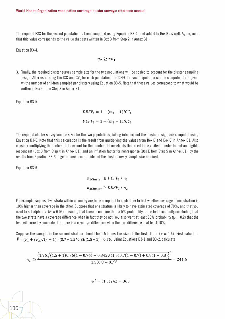
World Health Organization vaccination coverage cluster surveys: reference manual
136
The required ESS for the second population is then computed using Equation B3-4, and added to Box B as well. Again, note that this value corresponds to the value that gets written in Box B from Step 2 in Annex B1.
Equation B3-4.
B3-5
)- ≥)-E4 1 + 1 + 2(I + 1)
)-EI|?1 − ?-|
1
TherequiredESSforthesecondpopulationisthencomputedusingEquationB3-4,andaddedtoBoxBaswell.Again,notethatthisvaluecorrespondstothevaluethatgetswritteninBoxBfromStep2inAnnexB1.
EquationB3-4.)1 ≥ I)-
3. Finally,therequiredclustersurveysamplesizeforthetwopopulationswillbescaledtoaccountfortheclustersamplingdesign.AfterestimatingtheICCforeachpopulation,theDEFFforeachpopulationcanbecomputedforagivenM(thenumberofchildrensampledpercluster)usingEquationB3-5.NotethatthesevaluescorrespondtowhatwouldbewritteninBoxCfromStep3inAnnexB1.
EquationB3-5.N!OO- = 1 + M- − 1 PQQ-
N!OO1 = 1 + M1 − 1 PQQ1
Therequiredclustersurveysamplesizesforthetwopopulations,takingintoaccounttheclusterdesign,arecomputedusingEquationB3-6.NotethatthiscalculationistheresultfrommultiplyingthevaluesfromBoxBandBoxCinAnnexB1.Alsoconsidermultiplyingthefactorsthataccountforthenumberofhouseholdsthatneedtobevisitedinordertofindaneligiblerespondent(BoxDfromStep4inAnnexB1),andaninflationfactorfornonresponse(BoxEfromStep5inAnnexB1),bytheresultsfromEquationB3-6togetamoreaccurateideaoftheclustersurveysamplesizerequired.
EquationB3-6.
)-RSTUVWX ≥ N!OO- ∗ )-
)1RSTUVWX ≥ N!OO1 ∗ )1
Forexample,supposetwostratawithinacountryaretobecomparedtoeachothertotestwhethercoverageinonestratumis10%higherthancoverageintheother.Supposethatonestratumislikelytohaveestimatedcoverageof70%,andthatyouwanttosetalphaas(α=0.05),meaningthatthereisnomorethana5%probabilityofthetestincorrectlyconcludingthatthetwostratahaveacoveragedifferencewheninfacttheydonot.Youalsowantatleast80%probability(β=0.2)thatthetestwillcorrectlyconcludethatthereisacoveragedifferencewhenthetruedifferenceisatleast10%.
Supposethesampleinthesecondstratumshouldbe1.5timesthesizeofthefirststrata(r=1.5).Firstcalculate?=(?- + I?1)/(I + 1)=(0.7+1.5*0.8)/(1.5+1)=0.76.UsingEquationsB3-1andB3-2,calculate
3. Finally, the required cluster survey sample size for the two populations will be scaled to account for the cluster sampling design. After estimating the ICC and CVw for each population, the DEFF for each population can be computed for a given m (the number of children sampled per cluster) using Equation B3-5. Note that these values correspond to what would be written in Box C from Step 3 in Annex B1.
Equation B3-5.
B3-5
)- ≥)-E4 1 + 1 + 2(I + 1)
)-EI|?1 − ?-|
1
TherequiredESSforthesecondpopulationisthencomputedusingEquationB3-4,andaddedtoBoxBaswell.Again,notethatthisvaluecorrespondstothevaluethatgetswritteninBoxBfromStep2inAnnexB1.
EquationB3-4.)1 ≥ I)-
3. Finally,therequiredclustersurveysamplesizeforthetwopopulationswillbescaledtoaccountfortheclustersamplingdesign.AfterestimatingtheICCforeachpopulation,theDEFFforeachpopulationcanbecomputedforagivenM(thenumberofchildrensampledpercluster)usingEquationB3-5.NotethatthesevaluescorrespondtowhatwouldbewritteninBoxCfromStep3inAnnexB1.
EquationB3-5.N!OO- = 1 + M- − 1 PQQ-
N!OO1 = 1 + M1 − 1 PQQ1
Therequiredclustersurveysamplesizesforthetwopopulations,takingintoaccounttheclusterdesign,arecomputedusingEquationB3-6.NotethatthiscalculationistheresultfrommultiplyingthevaluesfromBoxBandBoxCinAnnexB1.Alsoconsidermultiplyingthefactorsthataccountforthenumberofhouseholdsthatneedtobevisitedinordertofindaneligiblerespondent(BoxDfromStep4inAnnexB1),andaninflationfactorfornonresponse(BoxEfromStep5inAnnexB1),bytheresultsfromEquationB3-6togetamoreaccurateideaoftheclustersurveysamplesizerequired.
EquationB3-6.
)-RSTUVWX ≥ N!OO- ∗ )-
)1RSTUVWX ≥ N!OO1 ∗ )1
Forexample,supposetwostratawithinacountryaretobecomparedtoeachothertotestwhethercoverageinonestratumis10%higherthancoverageintheother.Supposethatonestratumislikelytohaveestimatedcoverageof70%,andthatyouwanttosetalphaas(α=0.05),meaningthatthereisnomorethana5%probabilityofthetestincorrectlyconcludingthatthetwostratahaveacoveragedifferencewheninfacttheydonot.Youalsowantatleast80%probability(β=0.2)thatthetestwillcorrectlyconcludethatthereisacoveragedifferencewhenthetruedifferenceisatleast10%.
Supposethesampleinthesecondstratumshouldbe1.5timesthesizeofthefirststrata(r=1.5).Firstcalculate?=(?- + I?1)/(I + 1)=(0.7+1.5*0.8)/(1.5+1)=0.76.UsingEquationsB3-1andB3-2,calculate
The required cluster survey sample sizes for the two populations, taking into account the cluster design, are computed using Equation B3-6. Note that this calculation is the result from multiplying the values from Box B and Box C in Annex B1. Also consider multiplying the factors that account for the number of households that need to be visited in order to find an eligible respondent (Box D from Step 4 in Annex B1), and an inflation factor for nonresponse (Box E from Step 5 in Annex B1), by the results from Equation B3-6 to get a more accurate idea of the cluster survey sample size required.
Equation B3-6.
B3-5
)- ≥)-E4 1 + 1 + 2(I + 1)
)-EI|?1 − ?-|
1
TherequiredESSforthesecondpopulationisthencomputedusingEquationB3-4,andaddedtoBoxBaswell.Again,notethatthisvaluecorrespondstothevaluethatgetswritteninBoxBfromStep2inAnnexB1.
EquationB3-4.)1 ≥ I)-
3. Finally,therequiredclustersurveysamplesizeforthetwopopulationswillbescaledtoaccountfortheclustersamplingdesign.AfterestimatingtheICCforeachpopulation,theDEFFforeachpopulationcanbecomputedforagivenM(thenumberofchildrensampledpercluster)usingEquationB3-5.NotethatthesevaluescorrespondtowhatwouldbewritteninBoxCfromStep3inAnnexB1.
EquationB3-5.N!OO- = 1 + M- − 1 PQQ-
N!OO1 = 1 + M1 − 1 PQQ1
Therequiredclustersurveysamplesizesforthetwopopulations,takingintoaccounttheclusterdesign,arecomputedusingEquationB3-6.NotethatthiscalculationistheresultfrommultiplyingthevaluesfromBoxBandBoxCinAnnexB1.Alsoconsidermultiplyingthefactorsthataccountforthenumberofhouseholdsthatneedtobevisitedinordertofindaneligiblerespondent(BoxDfromStep4inAnnexB1),andaninflationfactorfornonresponse(BoxEfromStep5inAnnexB1),bytheresultsfromEquationB3-6togetamoreaccurateideaoftheclustersurveysamplesizerequired.
EquationB3-6.
)-RSTUVWX ≥ N!OO- ∗ )-
)1RSTUVWX ≥ N!OO1 ∗ )1
Forexample,supposetwostratawithinacountryaretobecomparedtoeachothertotestwhethercoverageinonestratumis10%higherthancoverageintheother.Supposethatonestratumislikelytohaveestimatedcoverageof70%,andthatyouwanttosetalphaas(α=0.05),meaningthatthereisnomorethana5%probabilityofthetestincorrectlyconcludingthatthetwostratahaveacoveragedifferencewheninfacttheydonot.Youalsowantatleast80%probability(β=0.2)thatthetestwillcorrectlyconcludethatthereisacoveragedifferencewhenthetruedifferenceisatleast10%.
Supposethesampleinthesecondstratumshouldbe1.5timesthesizeofthefirststrata(r=1.5).Firstcalculate?=(?- + I?1)/(I + 1)=(0.7+1.5*0.8)/(1.5+1)=0.76.UsingEquationsB3-1andB3-2,calculate
For example, suppose two strata within a country are to be compared to each other to test whether coverage in one stratum is 10% higher than coverage in the other. Suppose that one stratum is likely to have estimated coverage of 70%, and that you want to set alpha as ( = 0.05), meaning that there is no more than a 5% probability of the test incorrectly concluding that the two strata have a coverage difference when in fact they do not. You also want at least 80% probability ( = 0.2) that the test will correctly conclude that there is a coverage difference when the true difference is at least 10%.
Suppose the sample in the second stratum should be 1.5 times the size of the first strata (r = 1.5). First calculate
B3-5
)- ≥)-E4 1 + 1 + 2(I + 1)
)-EI|?1 − ?-|
1
TherequiredESSforthesecondpopulationisthencomputedusingEquationB3-4,andaddedtoBoxBaswell.Again,notethatthisvaluecorrespondstothevaluethatgetswritteninBoxBfromStep2inAnnexB1.
EquationB3-4.)1 ≥ I)-
3. Finally,therequiredclustersurveysamplesizeforthetwopopulationswillbescaledtoaccountfortheclustersamplingdesign.AfterestimatingtheICCforeachpopulation,theDEFFforeachpopulationcanbecomputedforagivenM(thenumberofchildrensampledpercluster)usingEquationB3-5.NotethatthesevaluescorrespondtowhatwouldbewritteninBoxCfromStep3inAnnexB1.
EquationB3-5.N!OO- = 1 + M- − 1 PQQ-
N!OO1 = 1 + M1 − 1 PQQ1
Therequiredclustersurveysamplesizesforthetwopopulations,takingintoaccounttheclusterdesign,arecomputedusingEquationB3-6.NotethatthiscalculationistheresultfrommultiplyingthevaluesfromBoxBandBoxCinAnnexB1.Alsoconsidermultiplyingthefactorsthataccountforthenumberofhouseholdsthatneedtobevisitedinordertofindaneligiblerespondent(BoxDfromStep4inAnnexB1),andaninflationfactorfornonresponse(BoxEfromStep5inAnnexB1),bytheresultsfromEquationB3-6togetamoreaccurateideaoftheclustersurveysamplesizerequired.
EquationB3-6.
)-RSTUVWX ≥ N!OO- ∗ )-
)1RSTUVWX ≥ N!OO1 ∗ )1
Forexample,supposetwostratawithinacountryaretobecomparedtoeachothertotestwhethercoverageinonestratumis10%higherthancoverageintheother.Supposethatonestratumislikelytohaveestimatedcoverageof70%,andthatyouwanttosetalphaas(α=0.05),meaningthatthereisnomorethana5%probabilityofthetestincorrectlyconcludingthatthetwostratahaveacoveragedifferencewheninfacttheydonot.Youalsowantatleast80%probability(β=0.2)thatthetestwillcorrectlyconcludethatthereisacoveragedifferencewhenthetruedifferenceisatleast10%.
Supposethesampleinthesecondstratumshouldbe1.5timesthesizeofthefirststrata(r=1.5).Firstcalculate?=(?- + I?1)/(I + 1)=(0.7+1.5*0.8)/(1.5+1)=0.76.UsingEquationsB3-1andB3-2,calculate
Using Equations B3-1 and B3-2, calculate
B3-6
)-E ≥1.96 1.5 + 1 0.76 1 − 0.76 + 0.842 1.5 0.7 1 − 0.7 + 0.8 1 − 0.8
1
1.5 0.8 − 0.7 1 = 241.6
)1E = 1.5 242 = 363
Roundupandsubstitute)-E intoEquationB3-3andB3-4toget
)- ≥2424 1 + 1 + 2 1.5 + 1
294 1.5 0.8 − 0.7
1
= 258.4
)1 ≥ 1.5 259 = 388.5
Thus,afterroundinguptothenearestwholenumber,theESSforthefirststratumwithestimatedcoverageof70%is)-≥259andtheESSforthesecondstratumis)1≥389.(NotethatthesevaluescorrespondtovaluesthatcouldbewritteninBoxBinStep2inAnnexB1.Inordertoobtaintherequiredclustersurveysamplesize,theESSwouldneedtobemultipliedbyvaluescorrespondingtoBoxesCthroughEinAnnexB1.)
B3.2 Testing for an increase in coverage over time, when the earlier survey was conducted in the past Subjecttothewarningsdescribedaboveaboutthedifficultyofcomparingcoveragebetweentwosurveysconductedatdifferenttimesbydifferentteamsandmethods,thissectionoftheannexgivesguidanceforsizingasurveyfora1-sidedcomparisonbetweentwosurveyswithcoveragemeasuredatanearliertimeforoneofthesurveys.
Incontrasttothepreviouslydescribedcomparisons,thistaskoffersfarlessflexibility.Whentwosurveysaretobecomparedandoneofthemhasalreadybeenconducted,thenthereisnoflexibilityintheeffectivesamplesizeneededtomeettheinferentialgoalsofthecomparisonstudy,astheeffectivesamplesizefromthefirststudyisalreadylockedinandnotnegotiable.Iftheeffectivesamplesizerequiredofthesecondsurveytomeettheinferentialgoalsistoolargeandthereforetooexpensiveortimeconsuming,theinferentialgoalswillneedtobemodified.
Forexample,ifacountryisplanningtoconducttwofuturesurveysatdifferenttimepointssuchthattheresultscanbecompared,thesurveyplannerscoulddecideto(1)conducttwoequallysizedsurveys,(2)conductalargesurveyfirstandthenasmallersurveytofollowor(3)conductasmallersurveyatfirstandalargersurveylater.Dependingonthebudgetandthetimeline,thereisgreatflexibilityplanningthesetwosurveyssuchthattheinferentialgoalsaremet.Whenonesurveyhasalreadybeenconducted,
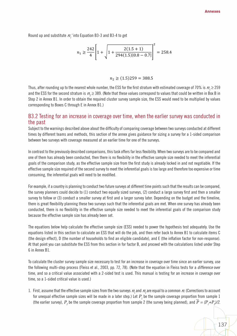
Annexes
137
Round up and substitute n1' into Equation B3-3 and B3-4 to get
B3-6
)-E ≥1.96 1.5 + 1 0.76 1 − 0.76 + 0.842 1.5 0.7 1 − 0.7 + 0.8 1 − 0.8
1
1.5 0.8 − 0.7 1 = 241.6
)1E = 1.5 242 = 363
Roundupandsubstitute)-E intoEquationB3-3andB3-4toget
)- ≥2424 1 + 1 + 2 1.5 + 1
294 1.5 0.8 − 0.7
1
= 258.4
)1 ≥ 1.5 259 = 388.5
Thus,afterroundinguptothenearestwholenumber,theESSforthefirststratumwithestimatedcoverageof70%is)-≥259andtheESSforthesecondstratumis)1≥389.(NotethatthesevaluescorrespondtovaluesthatcouldbewritteninBoxBinStep2inAnnexB1.Inordertoobtaintherequiredclustersurveysamplesize,theESSwouldneedtobemultipliedbyvaluescorrespondingtoBoxesCthroughEinAnnexB1.)
B3.2 Testing for an increase in coverage over time, when the earlier survey was conducted in the past Subjecttothewarningsdescribedaboveaboutthedifficultyofcomparingcoveragebetweentwosurveysconductedatdifferenttimesbydifferentteamsandmethods,thissectionoftheannexgivesguidanceforsizingasurveyfora1-sidedcomparisonbetweentwosurveyswithcoveragemeasuredatanearliertimeforoneofthesurveys.
Incontrasttothepreviouslydescribedcomparisons,thistaskoffersfarlessflexibility.Whentwosurveysaretobecomparedandoneofthemhasalreadybeenconducted,thenthereisnoflexibilityintheeffectivesamplesizeneededtomeettheinferentialgoalsofthecomparisonstudy,astheeffectivesamplesizefromthefirststudyisalreadylockedinandnotnegotiable.Iftheeffectivesamplesizerequiredofthesecondsurveytomeettheinferentialgoalsistoolargeandthereforetooexpensiveortimeconsuming,theinferentialgoalswillneedtobemodified.
Forexample,ifacountryisplanningtoconducttwofuturesurveysatdifferenttimepointssuchthattheresultscanbecompared,thesurveyplannerscoulddecideto(1)conducttwoequallysizedsurveys,(2)conductalargesurveyfirstandthenasmallersurveytofollowor(3)conductasmallersurveyatfirstandalargersurveylater.Dependingonthebudgetandthetimeline,thereisgreatflexibilityplanningthesetwosurveyssuchthattheinferentialgoalsaremet.Whenonesurveyhasalreadybeenconducted,
Thus, after rounding up to the nearest whole number, the ESS for the first stratum with estimated coverage of 70% is n1 ≥ 259 and the ESS for the second stratum is n2 ≥ 389. (Note that these values correspond to values that could be written in Box B in Step 2 in Annex B1. In order to obtain the required cluster survey sample size, the ESS would need to be multiplied by values corresponding to Boxes C through E in Annex B1.)
B3.2 Testing for an increase in coverage over time, when the earlier survey was conducted in the pastSubject to the warnings described above about the difficulty of comparing coverage between two surveys conducted at different times by different teams and methods, this section of the annex gives guidance for sizing a survey for a 1-sided comparison between two surveys with coverage measured at an earlier time for one of the surveys.
In contrast to the previously described comparisons, this task offers far less flexibility. When two surveys are to be compared and one of them has already been conducted, then there is no flexibility in the effective sample size needed to meet the inferential goals of the comparison study, as the effective sample size from the first study is already locked in and not negotiable. If the effective sample size required of the second survey to meet the inferential goals is too large and therefore too expensive or time consuming, the inferential goals will need to be modified.
For example, if a country is planning to conduct two future surveys at different time points such that the results can be compared, the survey planners could decide to (1) conduct two equally sized surveys, (2) conduct a large survey first and then a smaller survey to follow or (3) conduct a smaller survey at first and a larger survey later. Depending on the budget and the timeline, there is great flexibility planning these two surveys such that the inferential goals are met. When one survey has already been conducted, there is no flexibility in the effective sample size needed to meet the inferential goals of the comparison study because the effective sample size has already been set.
The equations below help calculate the effective sample size (ESS) needed to power the hypothesis test adequately. Use the equations listed in this section to calculate an ESS that will do the job, and then refer back to Annex B1 to calculate items C (the design effect), D (the number of households to find an eligible candidate), and E (the inflation factor for non-response). At that point you can substitute the ESS from this section in for factor B, and proceed with the calculations listed under Step 6 in Annex B1.
To calculate the cluster survey sample size necessary to test for an increase in coverage over time since an earlier survey, use the following multi-step process (Fleiss et al., 2003, pp. 72, 78). (Note that the equation in Fleiss tests for a difference over time, and so a critical value associated with a 2-sided test is used. This manual is testing for an increase in coverage over time, so a 1-sided critical value is used.)
1. First, assume that the effective sample sizes from the two surveys n1 and n2 are equal to a common n. (Corrections to account for unequal effective sample sizes will be made in a later step.) Let P1 be the sample coverage proportion from sample 1 (the earlier survey), P2 be the sample coverage proportion from sample 2 (the survey being planned), and P = (P1+P2)/2.
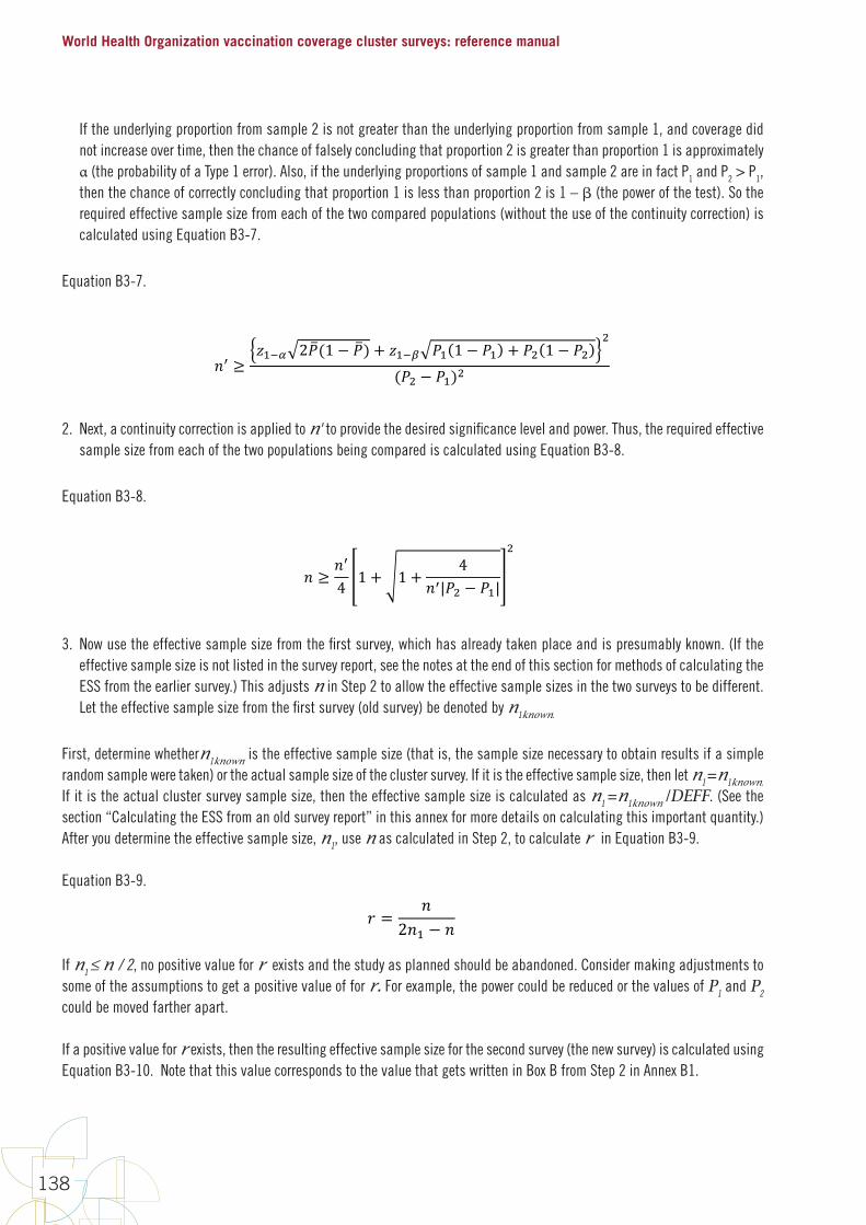
World Health Organization vaccination coverage cluster surveys: reference manual
138
If the underlying proportion from sample 2 is not greater than the underlying proportion from sample 1, and coverage did not increase over time, then the chance of falsely concluding that proportion 2 is greater than proportion 1 is approximately α (the probability of a Type 1 error). Also, if the underlying proportions of sample 1 and sample 2 are in fact P1 and P2 > P1, then the chance of correctly concluding that proportion 1 is less than proportion 2 is 1 – (the power of the test). So the required effective sample size from each of the two compared populations (without the use of the continuity correction) is calculated using Equation B3-7.
Equation B3-7.
B3-7
thereisnoflexibilityintheeffectivesamplesizeneededtomeettheinferentialgoalsofthecomparisonstudybecausetheeffectivesamplesizehasalreadybeenset.
Theequationsbelowhelpcalculatetheeffectivesamplesize(ESS)neededtopowerthehypothesistestadequately.UsetheequationslistedinthissectiontocalculateanESSthatwilldothejob,andthenreferbacktoAnnexB1tocalculateitemsC(thedesigneffect),D(thenumberofhouseholdstofindaneligiblecandidate),andE(theinflationfactorfornon-response).AtthatpointyoucansubstitutetheESSfromthissectioninforfactorB,andproceedwiththecalculationslistedunderStep6inAnnexB1.
Tocalculatetheclustersurveysamplesizenecessarytotestforanincreaseincoverageovertimesinceanearliersurvey,usethefollowingmulti-stepprocess(Fleissetal.,2003,pp.72,78).(NotethattheequationinFleisstestsforadifferenceovertime,andsoacriticalvalueassociatedwitha2-sidedtestisused.Thismanualistestingforanincreaseincoverageovertime,soa1-sidedcriticalvalueisused.)
1. First,assumethattheeffectivesamplesizesfromthetwosurveysn1andn2areequaltoacommonn.(Correctionstoaccountforunequaleffectivesamplesizeswillbemadeinalaterstep.)Let?-bethesamplecoverageproportionfromsample1(theearliersurvey),?1bethesamplecoverageproportionfromsample2(thesurveybeingplanned),and? = (?- + ?1)/2.Iftheunderlyingproportionfromsample2isnotgreaterthantheunderlyingproportionfromsample1,andcoveragedidnotincreaseovertime,thenthechanceoffalselyconcludingthatproportion2isgreaterthanproportion1isapproximatelyα(theprobabilityofaType1error).Also,iftheunderlyingproportionsofsample1andsample2areinfactP1andP2>P1,thenthechanceofcorrectlyconcludingthatproportion1islessthanproportion2is1–β(thepowerofthetest).Sotherequiredeffectivesamplesizefromeachofthetwocomparedpopulations(withouttheuseofthecontinuitycorrection)iscalculatedusingEquationB3-7.
EquationB3-7.
)E ≥,-./ 2?(1 − ?) + ,-.H ?- 1 − ?- + ?1 1 − ?1
1
(?1 − ?-)1
2. Next,acontinuitycorrectionisappliedto)Etoprovidethedesiredsignificancelevelandpower.Thus,therequiredeffectivesamplesizefromeachofthetwopopulationsbeingcomparediscalculatedusingEquationB3-8.
EquationB3-8.
) ≥ )E4 1 + 1 + 4
)E|?1 − ?-|
1
3. Nowusetheeffectivesamplesizefromthefirstsurvey,whichhasalreadytakenplaceandispresumablyknown.(Iftheeffectivesamplesizeisnotlistedinthesurveyreport,seethenotesattheendofthissectionformethodsofcalculatingtheESSfromtheearliersurvey.)Thisadjusts)inStep2toallowtheeffectivesamplesizesinthetwosurveystobedifferent.Lettheeffectivesamplesizefromthefirstsurvey(oldsurvey)bedenotedby)-[\]^\.
2. Next, a continuity correction is applied to n' to provide the desired significance level and power. Thus, the required effective sample size from each of the two populations being compared is calculated using Equation B3-8.
Equation B3-8.
B3-7
thereisnoflexibilityintheeffectivesamplesizeneededtomeettheinferentialgoalsofthecomparisonstudybecausetheeffectivesamplesizehasalreadybeenset.
Theequationsbelowhelpcalculatetheeffectivesamplesize(ESS)neededtopowerthehypothesistestadequately.UsetheequationslistedinthissectiontocalculateanESSthatwilldothejob,andthenreferbacktoAnnexB1tocalculateitemsC(thedesigneffect),D(thenumberofhouseholdstofindaneligiblecandidate),andE(theinflationfactorfornon-response).AtthatpointyoucansubstitutetheESSfromthissectioninforfactorB,andproceedwiththecalculationslistedunderStep6inAnnexB1.
Tocalculatetheclustersurveysamplesizenecessarytotestforanincreaseincoverageovertimesinceanearliersurvey,usethefollowingmulti-stepprocess(Fleissetal.,2003,pp.72,78).(NotethattheequationinFleisstestsforadifferenceovertime,andsoacriticalvalueassociatedwitha2-sidedtestisused.Thismanualistestingforanincreaseincoverageovertime,soa1-sidedcriticalvalueisused.)
1. First,assumethattheeffectivesamplesizesfromthetwosurveysn1andn2areequaltoacommonn.(Correctionstoaccountforunequaleffectivesamplesizeswillbemadeinalaterstep.)Let?-bethesamplecoverageproportionfromsample1(theearliersurvey),?1bethesamplecoverageproportionfromsample2(thesurveybeingplanned),and? = (?- + ?1)/2.Iftheunderlyingproportionfromsample2isnotgreaterthantheunderlyingproportionfromsample1,andcoveragedidnotincreaseovertime,thenthechanceoffalselyconcludingthatproportion2isgreaterthanproportion1isapproximatelyα(theprobabilityofaType1error).Also,iftheunderlyingproportionsofsample1andsample2areinfactP1andP2>P1,thenthechanceofcorrectlyconcludingthatproportion1islessthanproportion2is1–β(thepowerofthetest).Sotherequiredeffectivesamplesizefromeachofthetwocomparedpopulations(withouttheuseofthecontinuitycorrection)iscalculatedusingEquationB3-7.
EquationB3-7.
)E ≥,-./ 2?(1 − ?) + ,-.H ?- 1 − ?- + ?1 1 − ?1
1
(?1 − ?-)1
2. Next,acontinuitycorrectionisappliedto)Etoprovidethedesiredsignificancelevelandpower.Thus,therequiredeffectivesamplesizefromeachofthetwopopulationsbeingcomparediscalculatedusingEquationB3-8.
EquationB3-8.
) ≥ )E4 1 + 1 + 4
)E|?1 − ?-|
1
3. Nowusetheeffectivesamplesizefromthefirstsurvey,whichhasalreadytakenplaceandispresumablyknown.(Iftheeffectivesamplesizeisnotlistedinthesurveyreport,seethenotesattheendofthissectionformethodsofcalculatingtheESSfromtheearliersurvey.)Thisadjusts)inStep2toallowtheeffectivesamplesizesinthetwosurveystobedifferent.Lettheeffectivesamplesizefromthefirstsurvey(oldsurvey)bedenotedby)-[\]^\.
3. Now use the effective sample size from the first survey, which has already taken place and is presumably known. (If the effective sample size is not listed in the survey report, see the notes at the end of this section for methods of calculating the ESS from the earlier survey.) This adjusts n in Step 2 to allow the effective sample sizes in the two surveys to be different. Let the effective sample size from the first survey (old survey) be denoted by n1known.
First, determine whethern1known is the effective sample size (that is, the sample size necessary to obtain results if a simple random sample were taken) or the actual sample size of the cluster survey. If it is the effective sample size, then let n1 =n1known.
If it is the actual cluster survey sample size, then the effective sample size is calculated as n1 =n1known /DEFF. (See the section “Calculating the ESS from an old survey report” in this annex for more details on calculating this important quantity.) After you determine the effective sample size, n1, use n as calculated in Step 2, to calculate r in Equation B3-9.
Equation B3-9.
B3-8
First,determinewhether)-[\]^\istheeffectivesamplesize(thatis,thesamplesizenecessarytoobtainresultsifasimplerandomsampleweretaken)ortheactualsamplesizeoftheclustersurvey.Ifitistheeffectivesamplesize,thenlet)- = )-[\]^\.Ifitistheactualclustersurveysamplesize,thentheeffectivesamplesizeiscalculatedas)- = )-[\]^\/N!OO.(Seethesection“CalculatingtheESSfromanoldsurveyreport”inthisannexformoredetailsoncalculatingthisimportantquantity.)Afteryoudeterminetheeffectivesamplesize,)-,use)ascalculatedinStep2,tocalculateIinEquationB3-9.
EquationB3-9.
I = )2)- − )
If)- ≤ )/2,nopositivevalueforIexistsandthestudyasplannedshouldbeabandoned.ConsidermakingadjustmentstosomeoftheassumptionstogetapositivevalueofforI.Forexample,thepowercouldbereducedorthevaluesof?-and?1couldbemovedfartherapart.
IfapositivevalueforIexists,thentheresultingeffectivesamplesizeforthesecondsurvey(thenewsurvey)iscalculatedusingEquationB3-10.NotethatthisvaluecorrespondstothevaluethatgetswritteninBoxBfromStep2inAnnexB1.
EquationB3-10. )1 ≥ I ∗ )-
4. Finally,therequiredclustersurveysamplesizeforthesecondsurveywillbescaledtoaccountfortheclustersamplingdesign.AfterestimatingtheICC,calculatetheDEFFforagivenM(thenumberofchildrensampledpercluster)usingEquationB3-11.ThesevaluescorrespondtowhatwouldgetwritteninBoxCfromStep3inAnnexB1.
EquationB3-11.
N!OO = 1 + M − 1 PQQ
Theresultingclustersurveysamplesizeforthesecond(new)survey,takingintoaccounttheclusterdesign,iscomputedusingEquationB3-12.NotethatthiscalculationistheresultofmultiplyingthevaluesfromBoxBandBoxCinAnnexB1.Alsoconsidermultiplyingfactorsthataccountforthenumberofhouseholdsneededtothatneedtobevisitedinordertofindaneligiblerespondent(BoxDfromStep4inAnnexB1)andaninflationfactorfornonresponse(BoxEfromStep5inAnnexB1)bytheresultfromEquationB3-12,togetamoreaccurateclustersurveysamplesizefigure.
EquationB3-12.)1RSTUVWX ≥ N!OO ∗ )1
Forexample,supposeacountryconductedasurveyafewyearsagoandtheestimatedcoveragewas70%.Supposeitwasdesiredtoconductanothersurveyandtestifthecoveragehadincreasedovertimeto80%,withnomorethana5%probabilityofincorrectlyconcludingthatithadincreasedwheninfactithadnot(α=0.05),andatleast80%probabilityofcorrectlyconcludingthatithadincreased(β=0.2).Firstcalculate?=(0.7+0.8)/2=0.75.UsingtheequationinStep1,wecalculate
If n1 ≤ n / 2, no positive value for r exists and the study as planned should be abandoned. Consider making adjustments to some of the assumptions to get a positive value of for r. For example, the power could be reduced or the values of P1 and P2
could be moved farther apart.
If a positive value for r exists, then the resulting effective sample size for the second survey (the new survey) is calculated using Equation B3-10. Note that this value corresponds to the value that gets written in Box B from Step 2 in Annex B1.
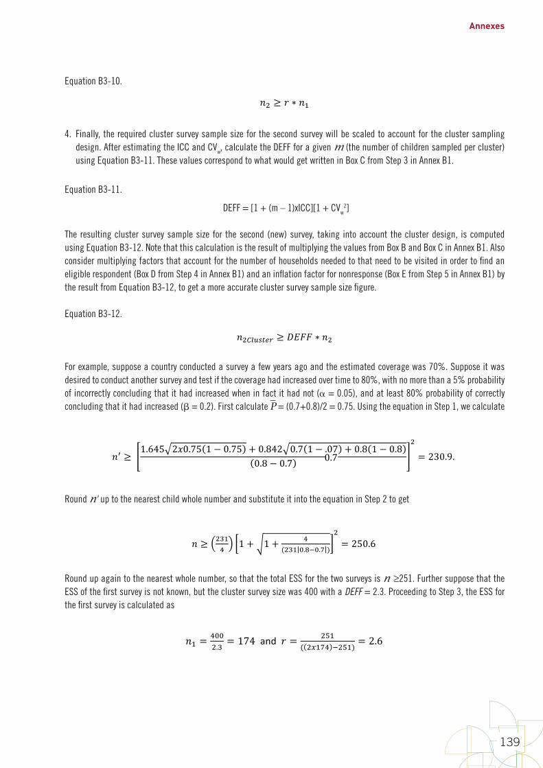
Annexes
139
Equation B3-10.
B3-8
First,determinewhether)-[\]^\istheeffectivesamplesize(thatis,thesamplesizenecessarytoobtainresultsifasimplerandomsampleweretaken)ortheactualsamplesizeoftheclustersurvey.Ifitistheeffectivesamplesize,thenlet)- = )-[\]^\.Ifitistheactualclustersurveysamplesize,thentheeffectivesamplesizeiscalculatedas)- = )-[\]^\/N!OO.(Seethesection“CalculatingtheESSfromanoldsurveyreport”inthisannexformoredetailsoncalculatingthisimportantquantity.)Afteryoudeterminetheeffectivesamplesize,)-,use)ascalculatedinStep2,tocalculateIinEquationB3-9.
EquationB3-9.
I = )2)- − )
If)- ≤ )/2,nopositivevalueforIexistsandthestudyasplannedshouldbeabandoned.ConsidermakingadjustmentstosomeoftheassumptionstogetapositivevalueofforI.Forexample,thepowercouldbereducedorthevaluesof?-and?1couldbemovedfartherapart.
IfapositivevalueforIexists,thentheresultingeffectivesamplesizeforthesecondsurvey(thenewsurvey)iscalculatedusingEquationB3-10.NotethatthisvaluecorrespondstothevaluethatgetswritteninBoxBfromStep2inAnnexB1.
EquationB3-10. )1 ≥ I ∗ )-
4. Finally,therequiredclustersurveysamplesizeforthesecondsurveywillbescaledtoaccountfortheclustersamplingdesign.AfterestimatingtheICC,calculatetheDEFFforagivenM(thenumberofchildrensampledpercluster)usingEquationB3-11.ThesevaluescorrespondtowhatwouldgetwritteninBoxCfromStep3inAnnexB1.
EquationB3-11.
N!OO = 1 + M − 1 PQQ
Theresultingclustersurveysamplesizeforthesecond(new)survey,takingintoaccounttheclusterdesign,iscomputedusingEquationB3-12.NotethatthiscalculationistheresultofmultiplyingthevaluesfromBoxBandBoxCinAnnexB1.Alsoconsidermultiplyingfactorsthataccountforthenumberofhouseholdsneededtothatneedtobevisitedinordertofindaneligiblerespondent(BoxDfromStep4inAnnexB1)andaninflationfactorfornonresponse(BoxEfromStep5inAnnexB1)bytheresultfromEquationB3-12,togetamoreaccurateclustersurveysamplesizefigure.
EquationB3-12.)1RSTUVWX ≥ N!OO ∗ )1
Forexample,supposeacountryconductedasurveyafewyearsagoandtheestimatedcoveragewas70%.Supposeitwasdesiredtoconductanothersurveyandtestifthecoveragehadincreasedovertimeto80%,withnomorethana5%probabilityofincorrectlyconcludingthatithadincreasedwheninfactithadnot(α=0.05),andatleast80%probabilityofcorrectlyconcludingthatithadincreased(β=0.2).Firstcalculate?=(0.7+0.8)/2=0.75.UsingtheequationinStep1,wecalculate
4. Finally, the required cluster survey sample size for the second survey will be scaled to account for the cluster sampling design. After estimating the ICC and CVw, calculate the DEFF for a given m (the number of children sampled per cluster) using Equation B3-11. These values correspond to what would get written in Box C from Step 3 in Annex B1.
Equation B3-11.
DEFF = [1 + (m – 1)xICC][1 + CVw2]
The resulting cluster survey sample size for the second (new) survey, taking into account the cluster design, is computed using Equation B3-12. Note that this calculation is the result of multiplying the values from Box B and Box C in Annex B1. Also consider multiplying factors that account for the number of households needed to that need to be visited in order to find an eligible respondent (Box D from Step 4 in Annex B1) and an inflation factor for nonresponse (Box E from Step 5 in Annex B1) by the result from Equation B3-12, to get a more accurate cluster survey sample size figure.
Equation B3-12.
B3-8
First,determinewhether)-[\]^\istheeffectivesamplesize(thatis,thesamplesizenecessarytoobtainresultsifasimplerandomsampleweretaken)ortheactualsamplesizeoftheclustersurvey.Ifitistheeffectivesamplesize,thenlet)- = )-[\]^\.Ifitistheactualclustersurveysamplesize,thentheeffectivesamplesizeiscalculatedas)- = )-[\]^\/N!OO.(Seethesection“CalculatingtheESSfromanoldsurveyreport”inthisannexformoredetailsoncalculatingthisimportantquantity.)Afteryoudeterminetheeffectivesamplesize,)-,use)ascalculatedinStep2,tocalculateIinEquationB3-9.
EquationB3-9.
I = )2)- − )
If)- ≤ )/2,nopositivevalueforIexistsandthestudyasplannedshouldbeabandoned.ConsidermakingadjustmentstosomeoftheassumptionstogetapositivevalueofforI.Forexample,thepowercouldbereducedorthevaluesof?-and?1couldbemovedfartherapart.
IfapositivevalueforIexists,thentheresultingeffectivesamplesizeforthesecondsurvey(thenewsurvey)iscalculatedusingEquationB3-10.NotethatthisvaluecorrespondstothevaluethatgetswritteninBoxBfromStep2inAnnexB1.
EquationB3-10. )1 ≥ I ∗ )-
4. Finally,therequiredclustersurveysamplesizeforthesecondsurveywillbescaledtoaccountfortheclustersamplingdesign.AfterestimatingtheICC,calculatetheDEFFforagivenM(thenumberofchildrensampledpercluster)usingEquationB3-11.ThesevaluescorrespondtowhatwouldgetwritteninBoxCfromStep3inAnnexB1.
EquationB3-11.
N!OO = 1 + M − 1 PQQ
Theresultingclustersurveysamplesizeforthesecond(new)survey,takingintoaccounttheclusterdesign,iscomputedusingEquationB3-12.NotethatthiscalculationistheresultofmultiplyingthevaluesfromBoxBandBoxCinAnnexB1.Alsoconsidermultiplyingfactorsthataccountforthenumberofhouseholdsneededtothatneedtobevisitedinordertofindaneligiblerespondent(BoxDfromStep4inAnnexB1)andaninflationfactorfornonresponse(BoxEfromStep5inAnnexB1)bytheresultfromEquationB3-12,togetamoreaccurateclustersurveysamplesizefigure.
EquationB3-12.)1RSTUVWX ≥ N!OO ∗ )1
Forexample,supposeacountryconductedasurveyafewyearsagoandtheestimatedcoveragewas70%.Supposeitwasdesiredtoconductanothersurveyandtestifthecoveragehadincreasedovertimeto80%,withnomorethana5%probabilityofincorrectlyconcludingthatithadincreasedwheninfactithadnot(α=0.05),andatleast80%probabilityofcorrectlyconcludingthatithadincreased(β=0.2).Firstcalculate?=(0.7+0.8)/2=0.75.UsingtheequationinStep1,wecalculate
For example, suppose a country conducted a survey a few years ago and the estimated coverage was 70%. Suppose it was desired to conduct another survey and test if the coverage had increased over time to 80%, with no more than a 5% probability of incorrectly concluding that it had increased when in fact it had not ( = 0.05), and at least 80% probability of correctly concluding that it had increased ( = 0.2). First calculate P = (0.7+0.8)/2 = 0.75. Using the equation in Step 1, we calculate
B3-9
)E ≥ 1.645 260.75 1 − 0.75 + 0.842 0.7 1 − .07 + 0.8 1 − 0.80.8 − 0.7
1
= 230.9.
Round)EuptothenearestchildwholenumberandsubstituteitintotheequationinStep2toget
) ≥ 1`-a 1 + 1 + a
(1`- @[email protected] )
1= 250.6
Roundupagaintothenearestwholenumber,sothatthetotalESSforthetwosurveysis)≥251.FurthersupposethattheESSofthefirstsurveyisnotknown,buttheclustersurveysizewas400withaDEFF=2.3.ProceedingtoStep3,theESSforthefirstsurveyiscalculatedas
)- =a@@1.` = 174andI = 1d-
( 15-ca .1d-) = 2.6
ThustheESSforthenewsurvey,roundinguptothenearestwholenumber,is)1≥2.6x174=453.
ThisistheESSneededfortheupcomingsurveytomeettheinferentialgoalsofthesurvey(thatis,thevaluefromBoxBinStep2inAnnexB1).Inordertoobtaintherequiredclustersurveysamplesize,theESSwouldneedtobemultipliedbythevaluescorrespondingtoBoxesCthroughEinAnnexB1.
Calculating the ESS from an old survey report Becausetheearliersurvey’seffectivesamplesizeisrequiredforthecalculationsdescribedabove,onepotentialchallengeishowtocalculateit.Usethefollowingequationstodoso,dependingontheinformationavailable.
• CalculateESSgivenNandDEFF:Ifthetotalclustersurveysamplesizeislisted,alongwiththedesigneffect(DEFF),thentheeffectivesamplesizeisthetotalsamplesizedividedbyDEFF.
• CalculateESSgivenNandDEFT:SometimesratherthanreportingDEFF,DHSandothersurveysreportDEFT,whichisthesquarerootofDEFF.InthatcasetheeffectivesamplesizeisthetotalsamplesizedividedbyDEFT-squared.
• CalculateESSgivenN,p1,andthe95%CI:IftheDEFFisnotlisted,butasymmetricalWald95%confidenceintervalforvaccinationcoverageislisted,alongwiththetotalsurveysamplesize,then:o LetNbethetotalclustersurveysamplesizefromwhichcoveragewascalculatedinthe
earliersurvey.o Letp1bethesurveycoverageestimatefromtheearliersurvey,dividedby100:80%/100%
=0.8.o LetFCW(fullconfidencewidth)equalthefullwidthofthe95%confidenceinterval,
expressedinproportions,soaCIof63%to73%wouldbeaFCWof(73%–63%)/100%=0.1.
Round n' up to the nearest child whole number and substitute it into the equation in Step 2 to get
B3-9
)E ≥ 1.645 260.75 1 − 0.75 + 0.842 0.7 1 − .07 + 0.8 1 − 0.80.8 − 0.7
1
= 230.9.
Round)EuptothenearestchildwholenumberandsubstituteitintotheequationinStep2toget
) ≥ 1`-a 1 + 1 + a
(1`- @[email protected] )
1= 250.6
Roundupagaintothenearestwholenumber,sothatthetotalESSforthetwosurveysis)≥251.FurthersupposethattheESSofthefirstsurveyisnotknown,buttheclustersurveysizewas400withaDEFF=2.3.ProceedingtoStep3,theESSforthefirstsurveyiscalculatedas
)- =a@@1.` = 174andI = 1d-
( 15-ca .1d-) = 2.6
ThustheESSforthenewsurvey,roundinguptothenearestwholenumber,is)1≥2.6x174=453.
ThisistheESSneededfortheupcomingsurveytomeettheinferentialgoalsofthesurvey(thatis,thevaluefromBoxBinStep2inAnnexB1).Inordertoobtaintherequiredclustersurveysamplesize,theESSwouldneedtobemultipliedbythevaluescorrespondingtoBoxesCthroughEinAnnexB1.
Calculating the ESS from an old survey report Becausetheearliersurvey’seffectivesamplesizeisrequiredforthecalculationsdescribedabove,onepotentialchallengeishowtocalculateit.Usethefollowingequationstodoso,dependingontheinformationavailable.
• CalculateESSgivenNandDEFF:Ifthetotalclustersurveysamplesizeislisted,alongwiththedesigneffect(DEFF),thentheeffectivesamplesizeisthetotalsamplesizedividedbyDEFF.
• CalculateESSgivenNandDEFT:SometimesratherthanreportingDEFF,DHSandothersurveysreportDEFT,whichisthesquarerootofDEFF.InthatcasetheeffectivesamplesizeisthetotalsamplesizedividedbyDEFT-squared.
• CalculateESSgivenN,p1,andthe95%CI:IftheDEFFisnotlisted,butasymmetricalWald95%confidenceintervalforvaccinationcoverageislisted,alongwiththetotalsurveysamplesize,then:o LetNbethetotalclustersurveysamplesizefromwhichcoveragewascalculatedinthe
earliersurvey.o Letp1bethesurveycoverageestimatefromtheearliersurvey,dividedby100:80%/100%
=0.8.o LetFCW(fullconfidencewidth)equalthefullwidthofthe95%confidenceinterval,
expressedinproportions,soaCIof63%to73%wouldbeaFCWof(73%–63%)/100%=0.1.
Round up again to the nearest whole number, so that the total ESS for the two surveys is n ≥251. Further suppose that the ESS of the first survey is not known, but the cluster survey size was 400 with a DEFF = 2.3. Proceeding to Step 3, the ESS for the first survey is calculated as
B3-9
)E ≥ 1.645 260.75 1 − 0.75 + 0.842 0.7 1 − .07 + 0.8 1 − 0.80.8 − 0.7
1
= 230.9.
Round)EuptothenearestchildwholenumberandsubstituteitintotheequationinStep2toget
) ≥ 1`-a 1 + 1 + a
(1`- @[email protected] )
1= 250.6
Roundupagaintothenearestwholenumber,sothatthetotalESSforthetwosurveysis)≥251.FurthersupposethattheESSofthefirstsurveyisnotknown,buttheclustersurveysizewas400withaDEFF=2.3.ProceedingtoStep3,theESSforthefirstsurveyiscalculatedas
)- =a@@1.` = 174andI = 1d-
( 15-ca .1d-) = 2.6
ThustheESSforthenewsurvey,roundinguptothenearestwholenumber,is)1≥2.6x174=453.
ThisistheESSneededfortheupcomingsurveytomeettheinferentialgoalsofthesurvey(thatis,thevaluefromBoxBinStep2inAnnexB1).Inordertoobtaintherequiredclustersurveysamplesize,theESSwouldneedtobemultipliedbythevaluescorrespondingtoBoxesCthroughEinAnnexB1.
Calculating the ESS from an old survey report Becausetheearliersurvey’seffectivesamplesizeisrequiredforthecalculationsdescribedabove,onepotentialchallengeishowtocalculateit.Usethefollowingequationstodoso,dependingontheinformationavailable.
• CalculateESSgivenNandDEFF:Ifthetotalclustersurveysamplesizeislisted,alongwiththedesigneffect(DEFF),thentheeffectivesamplesizeisthetotalsamplesizedividedbyDEFF.
• CalculateESSgivenNandDEFT:SometimesratherthanreportingDEFF,DHSandothersurveysreportDEFT,whichisthesquarerootofDEFF.InthatcasetheeffectivesamplesizeisthetotalsamplesizedividedbyDEFT-squared.
• CalculateESSgivenN,p1,andthe95%CI:IftheDEFFisnotlisted,butasymmetricalWald95%confidenceintervalforvaccinationcoverageislisted,alongwiththetotalsurveysamplesize,then:o LetNbethetotalclustersurveysamplesizefromwhichcoveragewascalculatedinthe
earliersurvey.o Letp1bethesurveycoverageestimatefromtheearliersurvey,dividedby100:80%/100%
=0.8.o LetFCW(fullconfidencewidth)equalthefullwidthofthe95%confidenceinterval,
expressedinproportions,soaCIof63%to73%wouldbeaFCWof(73%–63%)/100%=0.1.
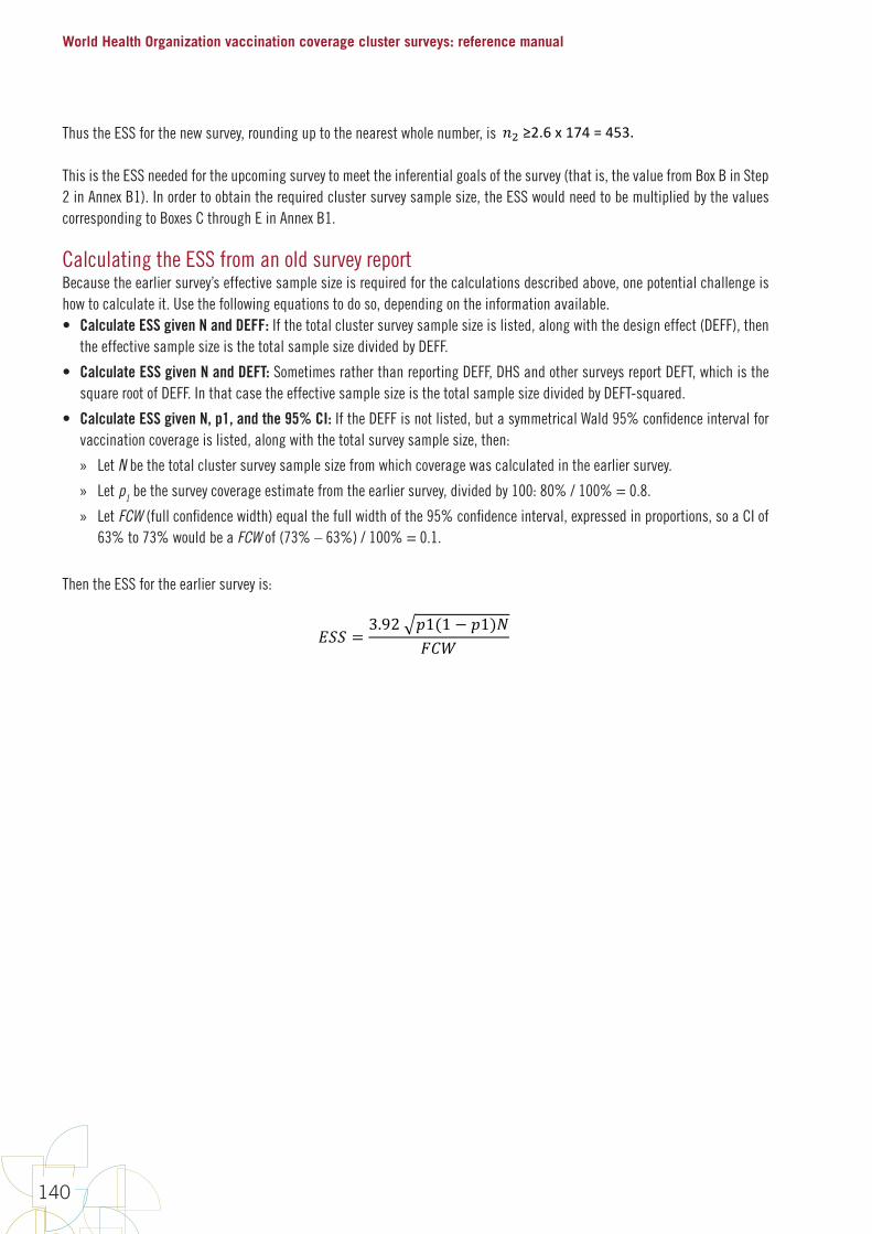
World Health Organization vaccination coverage cluster surveys: reference manual
140
Thus the ESS for the new survey, rounding up to the nearest whole number, is
B3-9
)E ≥ 1.645 260.75 1 − 0.75 + 0.842 0.7 1 − .07 + 0.8 1 − 0.80.8 − 0.7
1
= 230.9.
Round)EuptothenearestchildwholenumberandsubstituteitintotheequationinStep2toget
) ≥ 1`-a 1 + 1 + a
(1`- @[email protected] )
1= 250.6
Roundupagaintothenearestwholenumber,sothatthetotalESSforthetwosurveysis)≥251.FurthersupposethattheESSofthefirstsurveyisnotknown,buttheclustersurveysizewas400withaDEFF=2.3.ProceedingtoStep3,theESSforthefirstsurveyiscalculatedas
)- =a@@1.` = 174andI = 1d-
( 15-ca .1d-) = 2.6
ThustheESSforthenewsurvey,roundinguptothenearestwholenumber,is)1≥2.6x174=453.
ThisistheESSneededfortheupcomingsurveytomeettheinferentialgoalsofthesurvey(thatis,thevaluefromBoxBinStep2inAnnexB1).Inordertoobtaintherequiredclustersurveysamplesize,theESSwouldneedtobemultipliedbythevaluescorrespondingtoBoxesCthroughEinAnnexB1.
Calculating the ESS from an old survey report Becausetheearliersurvey’seffectivesamplesizeisrequiredforthecalculationsdescribedabove,onepotentialchallengeishowtocalculateit.Usethefollowingequationstodoso,dependingontheinformationavailable.
• CalculateESSgivenNandDEFF:Ifthetotalclustersurveysamplesizeislisted,alongwiththedesigneffect(DEFF),thentheeffectivesamplesizeisthetotalsamplesizedividedbyDEFF.
• CalculateESSgivenNandDEFT:SometimesratherthanreportingDEFF,DHSandothersurveysreportDEFT,whichisthesquarerootofDEFF.InthatcasetheeffectivesamplesizeisthetotalsamplesizedividedbyDEFT-squared.
• CalculateESSgivenN,p1,andthe95%CI:IftheDEFFisnotlisted,butasymmetricalWald95%confidenceintervalforvaccinationcoverageislisted,alongwiththetotalsurveysamplesize,then:o LetNbethetotalclustersurveysamplesizefromwhichcoveragewascalculatedinthe
earliersurvey.o Letp1bethesurveycoverageestimatefromtheearliersurvey,dividedby100:80%/100%
=0.8.o LetFCW(fullconfidencewidth)equalthefullwidthofthe95%confidenceinterval,
expressedinproportions,soaCIof63%to73%wouldbeaFCWof(73%–63%)/100%=0.1.
This is the ESS needed for the upcoming survey to meet the inferential goals of the survey (that is, the value from Box B in Step 2 in Annex B1). In order to obtain the required cluster survey sample size, the ESS would need to be multiplied by the values corresponding to Boxes C through E in Annex B1.
Calculating the ESS from an old survey reportBecause the earlier survey’s effective sample size is required for the calculations described above, one potential challenge is how to calculate it. Use the following equations to do so, depending on the information available. • Calculate ESS given N and DEFF: If the total cluster survey sample size is listed, along with the design effect (DEFF), then
the effective sample size is the total sample size divided by DEFF.
• Calculate ESS given N and DEFT: Sometimes rather than reporting DEFF, DHS and other surveys report DEFT, which is the square root of DEFF. In that case the effective sample size is the total sample size divided by DEFT-squared.
• Calculate ESS given N, p1, and the 95% CI: If the DEFF is not listed, but a symmetrical Wald 95% confidence interval for vaccination coverage is listed, along with the total survey sample size, then:
» Let N be the total cluster survey sample size from which coverage was calculated in the earlier survey.
» Let p1 be the survey coverage estimate from the earlier survey, divided by 100: 80% / 100% = 0.8.
» Let FCW (full confidence width) equal the full width of the 95% confidence interval, expressed in proportions, so a CI of 63% to 73% would be a FCW of (73% – 63%) / 100% = 0.1.
Then the ESS for the earlier survey is:
B3-10
ThentheESSfortheearliersurveyis:
!"" = 3.92 e1(1 − e1)(OQf
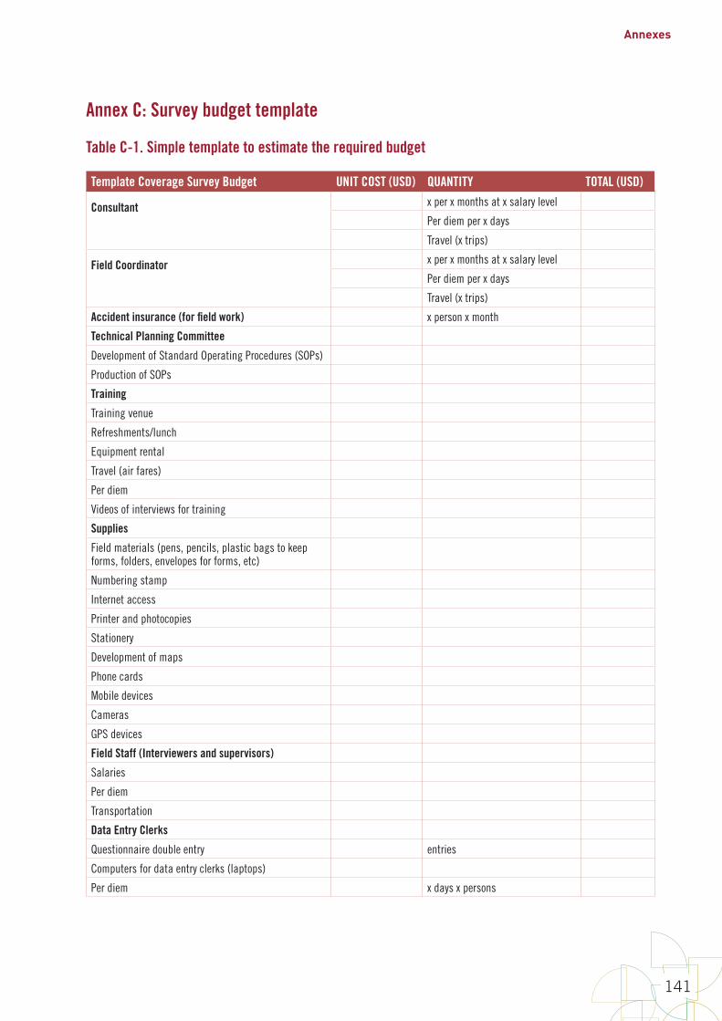
Annexes
141
Annex C: Survey budget template
Table C-1. Simple template to estimate the required budget
Template Coverage Survey Budget UNIT COST (USD) QUANTITY TOTAL (USD)
Consultant
x per x months at x salary level
Per diem per x days
Travel (x trips)
Field Coordinator
x per x months at x salary level
Per diem per x days
Travel (x trips)
Accident insurance (for field work) x person x month
Technical Planning Committee
Development of Standard Operating Procedures (SOPs)
Production of SOPs
Training
Training venue
Refreshments/lunch
Equipment rental
Travel (air fares)
Per diem
Videos of interviews for training
Supplies
Field materials (pens, pencils, plastic bags to keep forms, folders, envelopes for forms, etc)
Numbering stamp
Internet access
Printer and photocopies
Stationery
Development of maps
Phone cards
Mobile devices
Cameras
GPS devices
Field Staff (Interviewers and supervisors)
Salaries
Per diem
Transportation
Data Entry Clerks
Questionnaire double entry entries
Computers for data entry clerks (laptops)
Per diem x days x persons

World Health Organization vaccination coverage cluster surveys: reference manual
142
Template Coverage Survey Budget UNIT COST (USD) QUANTITY TOTAL (USD)Data Entry
Data entry clerks
Flash drives
Data Analysis
Contracting of statistician
Report Writing and Dissemination
Printing final report
Meeting logistics
Social mobilization
Media release
Dissemination meeting
Meeting venue
CDs or USBs
SUB-TOTAL
Coordination visits
Per diem x days x persons x trips
X trips x airfares
SUB-TOTAL
TOTAL
For more comprehensive and detailed budget templates see examples from:DHS: https://www.k4health.org/toolkits/dhs MICS: http://mics.unicef.org/tools
Annexes
143
Annex D: An example of systematic random cluster selection without replacement and probability proportional to estimated size (PPES)
D.1 IntroductionThis annex provides a worked example of how to randomly and systematically select, without replacement, 15 clusters for a survey in a given stratum, using probability proportional to the estimated number of households per cluster. The sampling frame consists of a list of census enumeration areas (EAs). In this example, they are numbered 1–45 by the census bureau.
If the sample had been done with replacement, it would mean that, theoretically, any EA could be selected into the sample two or more times. Because the sampling described here is systematic, and because we recommend segmenting large EAs so that none are sampled with certainty, the sampling here is without replacement. This annex discusses the benefits and disadvantages of sampling large clusters with certainty, and also gives tips for auditing the cluster selection process.
D.2 Example of cluster selectionThe example described in this section demonstrates cluster selection using systematic selection without replacement and demonstrates probability proportional to estimated size (PPES), with implicit urban/rural stratification and pre-segmentation of large clusters to avoid selection of any EA with certainty.
Implicitly stratify the sample
In this example, the survey designers have decided to stratify the sample implicitly by urban/rural status. That is, they want the ratio of urban to rural respondents in the survey to match the ratio of urban to rural population in each stratum. Implicit urban/rural stratification is usually a good idea; it makes the sample proportions representative of the population proportions, even if the survey is not examining urban vs. rural distinctions as a primary goal.
Table D-1 lists the 45 EAs in the stratum, along with the estimated number of households in each and an indicator for urban/rural status. Suppose that there will be 15 clusters in this survey, and that to yield an adequate number of completed questionnaires, the survey design calls for visiting 35 households in each cluster.
When using systematic sampling, first list the EAs in a pre-specified order to facilitate auditing later on. For this example, we will sort the list with all the urban EAs listed at the top and the rural EAs afterward. This creates an implicit urban/rural stratification. Within the urban and rural categories we will sort the list by EA number. Table D-2 shows the re-sorted table, with an additional column for cumulative number of households (HH).
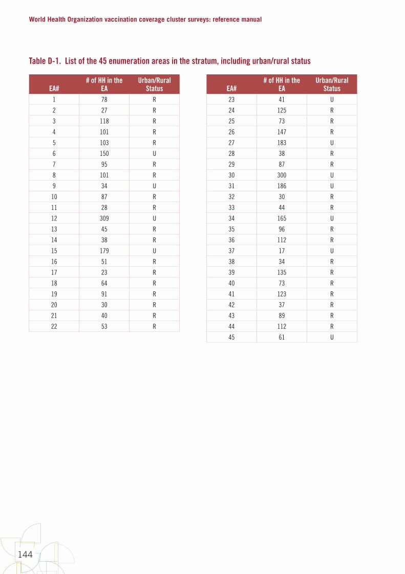
World Health Organization vaccination coverage cluster surveys: reference manual
144
Table D-1. List of the 45 enumeration areas in the stratum, including urban/rural status
EA## of HH in the
EAUrban/Rural
Status EA## of HH in the
EAUrban/Rural
Status1 78 R 23 41 U
2 27 R 24 125 R
3 118 R 25 73 R
4 101 R 26 147 R
5 103 R 27 183 U
6 150 U 28 38 R
7 95 R 29 87 R
8 101 R 30 300 U
9 34 U 31 186 U
10 87 R 32 30 R
11 28 R 33 44 R
12 309 U 34 165 U
13 45 R 35 96 R
14 38 R 36 112 R
15 179 U 37 17 U
16 51 R 38 34 R
17 23 R 39 135 R
18 64 R 40 73 R
19 91 R 41 123 R
20 30 R 42 37 R
21 40 R 43 89 R
22 53 R 44 112 R
45 61 U
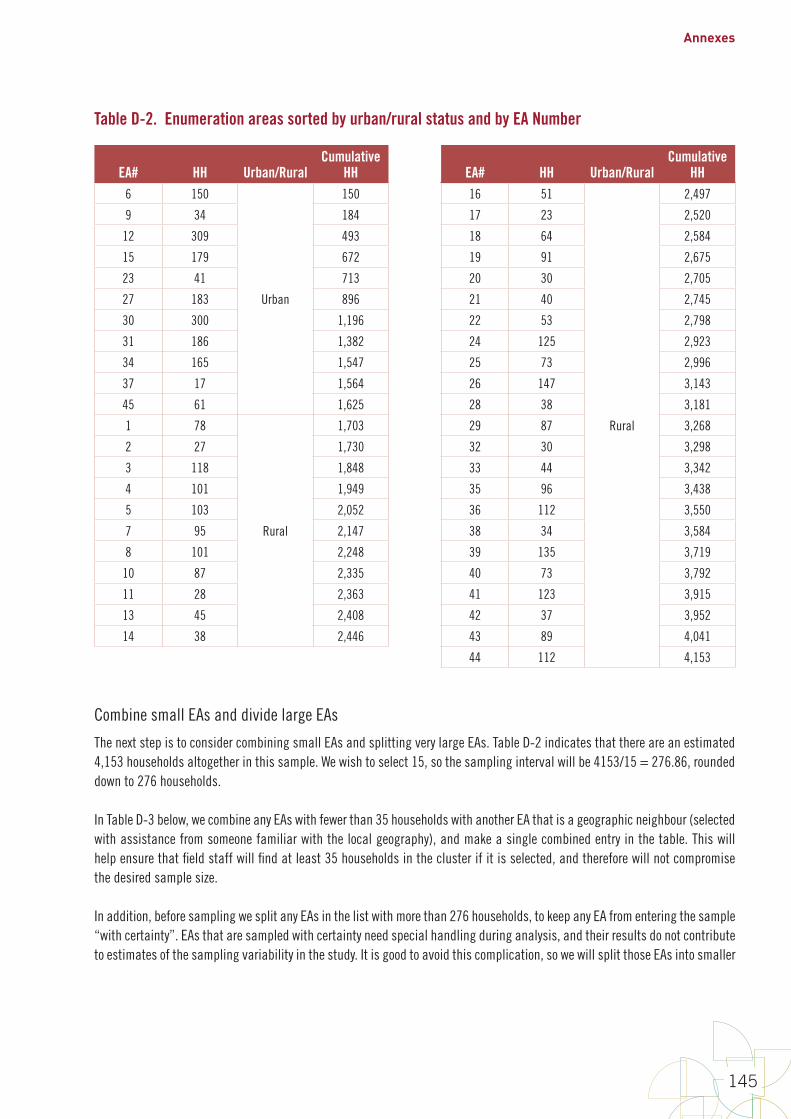
Annexes
145
Table D-2. Enumeration areas sorted by urban/rural status and by EA Number
EA# HH Urban/RuralCumulative
HH EA# HH Urban/RuralCumulative
HH6 150
Urban
150 16 51
Rural
2,497
9 34 184 17 23 2,520
12 309 493 18 64 2,584
15 179 672 19 91 2,675
23 41 713 20 30 2,705
27 183 896 21 40 2,745
30 300 1,196 22 53 2,798
31 186 1,382 24 125 2,923
34 165 1,547 25 73 2,996
37 17 1,564 26 147 3,143
45 61 1,625 28 38 3,181
1 78
Rural
1,703 29 87 3,268
2 27 1,730 32 30 3,298
3 118 1,848 33 44 3,342
4 101 1,949 35 96 3,438
5 103 2,052 36 112 3,550
7 95 2,147 38 34 3,584
8 101 2,248 39 135 3,719
10 87 2,335 40 73 3,792
11 28 2,363 41 123 3,915
13 45 2,408 42 37 3,952
14 38 2,446 43 89 4,041
44 112 4,153
Combine small EAs and divide large EAs
The next step is to consider combining small EAs and splitting very large EAs. Table D-2 indicates that there are an estimated 4,153 households altogether in this sample. We wish to select 15, so the sampling interval will be 4153/15 = 276.86, rounded down to 276 households.
In Table D-3 below, we combine any EAs with fewer than 35 households with another EA that is a geographic neighbour (selected with assistance from someone familiar with the local geography), and make a single combined entry in the table. This will help ensure that field staff will find at least 35 households in the cluster if it is selected, and therefore will not compromise the desired sample size.
In addition, before sampling we split any EAs in the list with more than 276 households, to keep any EA from entering the sample “with certainty”. EAs that are sampled with certainty need special handling during analysis, and their results do not contribute to estimates of the sampling variability in the study. It is good to avoid this complication, so we will split those EAs into smaller
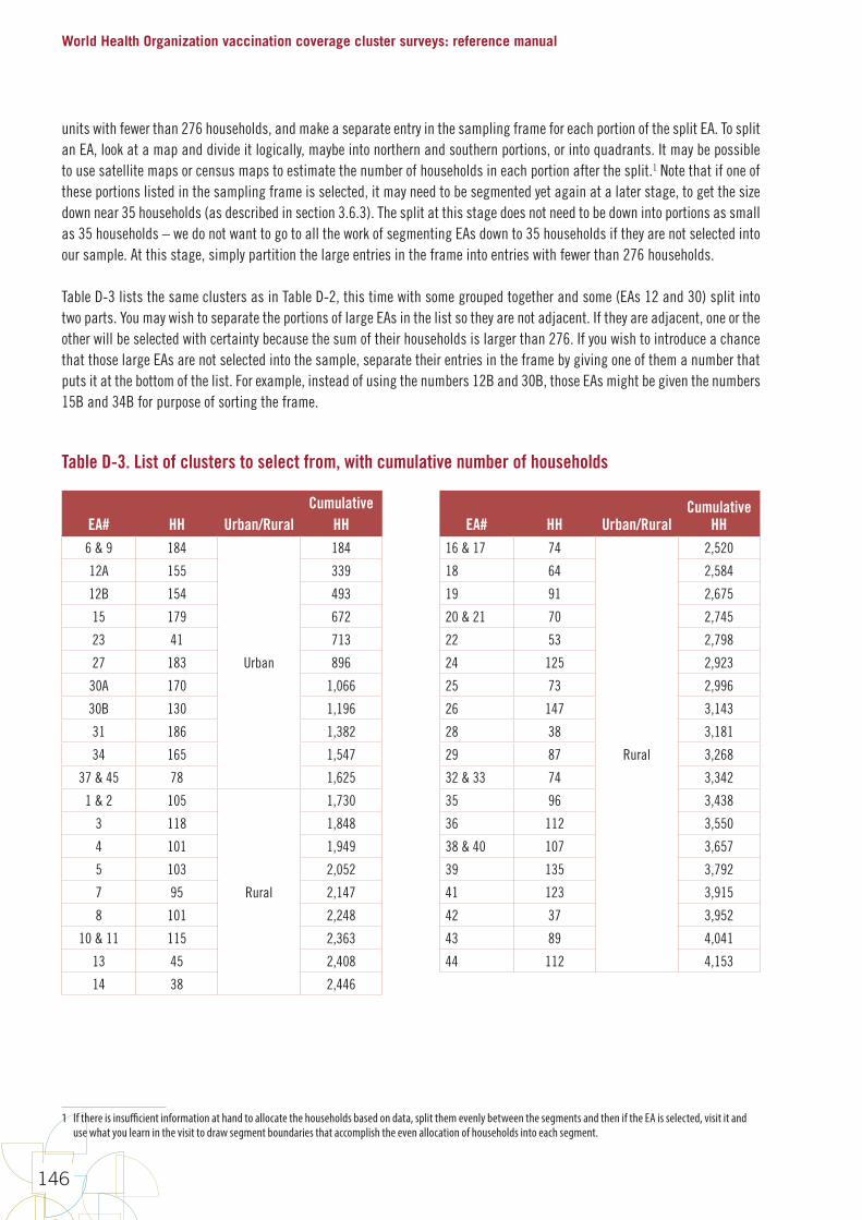
World Health Organization vaccination coverage cluster surveys: reference manual
146
units with fewer than 276 households, and make a separate entry in the sampling frame for each portion of the split EA. To split an EA, look at a map and divide it logically, maybe into northern and southern portions, or into quadrants. It may be possible to use satellite maps or census maps to estimate the number of households in each portion after the split.1 Note that if one of these portions listed in the sampling frame is selected, it may need to be segmented yet again at a later stage, to get the size down near 35 households (as described in section 3.6.3). The split at this stage does not need to be down into portions as small as 35 households – we do not want to go to all the work of segmenting EAs down to 35 households if they are not selected into our sample. At this stage, simply partition the large entries in the frame into entries with fewer than 276 households.
Table D-3 lists the same clusters as in Table D-2, this time with some grouped together and some (EAs 12 and 30) split into two parts. You may wish to separate the portions of large EAs in the list so they are not adjacent. If they are adjacent, one or the other will be selected with certainty because the sum of their households is larger than 276. If you wish to introduce a chance that those large EAs are not selected into the sample, separate their entries in the frame by giving one of them a number that puts it at the bottom of the list. For example, instead of using the numbers 12B and 30B, those EAs might be given the numbers 15B and 34B for purpose of sorting the frame.
Table D-3. List of clusters to select from, with cumulative number of households
EA# HH Urban/RuralCumulative
HH EA# HH Urban/RuralCumulative
HH6 & 9 184
Urban
184 16 & 17 74
Rural
2,520
12A 155 339 18 64 2,584
12B 154 493 19 91 2,675
15 179 672 20 & 21 70 2,745
23 41 713 22 53 2,798
27 183 896 24 125 2,923
30A 170 1,066 25 73 2,996
30B 130 1,196 26 147 3,143
31 186 1,382 28 38 3,181
34 165 1,547 29 87 3,268
37 & 45 78 1,625 32 & 33 74 3,342
1 & 2 105
Rural
1,730 35 96 3,438
3 118 1,848 36 112 3,550
4 101 1,949 38 & 40 107 3,657
5 103 2,052 39 135 3,792
7 95 2,147 41 123 3,915
8 101 2,248 42 37 3,952
10 & 11 115 2,363 43 89 4,041
13 45 2,408 44 112 4,153
14 38 2,446
1 If there is insufficient information at hand to allocate the households based on data, split them evenly between the segments and then if the EA is selected, visit it and use what you learn in the visit to draw segment boundaries that accomplish the even allocation of households into each segment.

Annexes
147
Select clusters
We are ready to begin selecting clusters. The next step is to select a random number between 1 and 276 and identify which cluster it falls in. To select the random number, you can use Microsoft Excel with the formula =RANDBETWEEN(1,276). Be sure to record the result somewhere for the permanent record, as the random number will change every time you refresh.
In this example, assume the equation yielded a random starting number of 107. The household with cumulative number 107 falls in EA 6 and 9. This is the first cluster selected for our sample. The second is identified by adding 276 (the sampling interval) to 107, which yields 383. Household 383 falls in EA #12B. We go on adding 276 to the running total time after time, until we have selected a total of 15 numbers systematically. Table D-4 shows which 15 clusters were selected.
Table D-4. List of clusters to select from, and those selected
EA# HH Urban/RuralCumulative
HH
Selected HH#After adding the sampling interval
(Running Sum) Cluster ID6 & 9 184
Urban
184 107 1
12A 155 339
12B 154 493 383 2
15 179 672 659 3
23 41 713
27 183 896
30A 170 1,066 935 4
30B 130 1,196
31 186 1,382 1,211 5
34 165 1,547 1,487 6
37 & 45 78 1,625
1 & 2 105
Rural
1,730
3 118 1,848 1,763 7
4 101 1,949
5 103 2,052 2,039 8
7 95 2,147
8 101 2,248
10 & 11 115 2,363 2,315 9
13 45 2,408
14 38 2,446
16 & 17 74 2,520
18 64 2,584
19 91 2,675 2,591 10
20 & 21 70 2,745
22 53 2,798
24 125 2,923 2,867 11
25 73 2,996
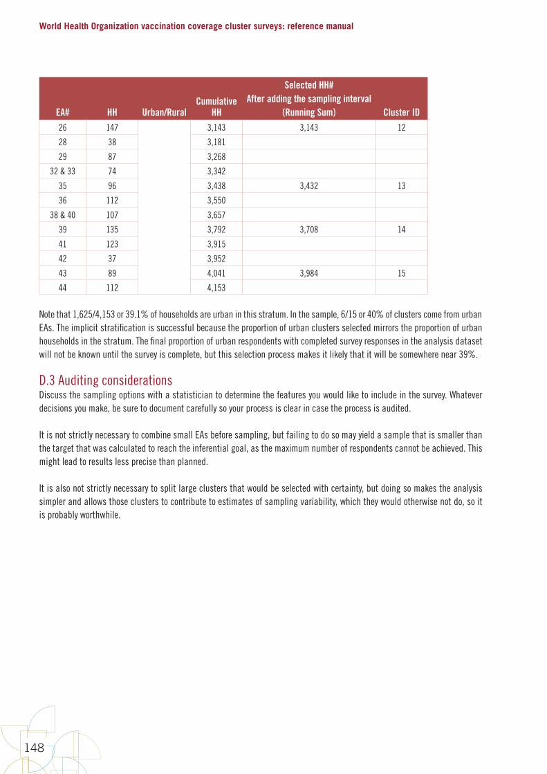
World Health Organization vaccination coverage cluster surveys: reference manual
148
EA# HH Urban/RuralCumulative
HH
Selected HH#After adding the sampling interval
(Running Sum) Cluster ID26 147 3,143 3,143 12
28 38 3,181
29 87 3,268
32 & 33 74 3,342
35 96 3,438 3,432 13
36 112 3,550
38 & 40 107 3,657
39 135 3,792 3,708 14
41 123 3,915
42 37 3,952
43 89 4,041 3,984 15
44 112 4,153
Note that 1,625/4,153 or 39.1% of households are urban in this stratum. In the sample, 6/15 or 40% of clusters come from urban EAs. The implicit stratification is successful because the proportion of urban clusters selected mirrors the proportion of urban households in the stratum. The final proportion of urban respondents with completed survey responses in the analysis dataset will not be known until the survey is complete, but this selection process makes it likely that it will be somewhere near 39%.
D.3 Auditing considerationsDiscuss the sampling options with a statistician to determine the features you would like to include in the survey. Whatever decisions you make, be sure to document carefully so your process is clear in case the process is audited.
It is not strictly necessary to combine small EAs before sampling, but failing to do so may yield a sample that is smaller than the target that was calculated to reach the inferential goal, as the maximum number of respondents cannot be achieved. This might lead to results less precise than planned.
It is also not strictly necessary to split large clusters that would be selected with certainty, but doing so makes the analysis simpler and allows those clusters to contribute to estimates of sampling variability, which they would otherwise not do, so it is probably worthwhile.
Annexes
149
Finally, it is not strictly necessary to use systematic random sampling. Any other system of probability sampling would be acceptable, but systematic sampling has the advantage that the method is easy to audit. Anyone can re-open the spreadsheet and examine the random number, sampling interval, and selected clusters. Sort clusters in alphabetic order by EA name or numeric order by EA identifier, so there is no possibility whatsoever that anyone could tamper with the cluster selection list and hand pick the clusters in the sampling plan.2 An audit of tampered cluster selection would show that the sample frame was not sorted properly from the start, or that the sampling interval was not respected. Therefore, systematic sampling is advisable if the survey steering committee wishes to audit the cluster selection process and ensure that clusters are selected in a random fashion.
D.4 Weighting considerationsRegardless of the method used for random cluster sampling, the materials used to select clusters should be made available to the project statistician to use when calculating sampling weights. The probability of selection for each cluster must be calculable, as they are used to calculate weights. If EAs were combined or split, that information must be available, too.
If applicable, the materials used to further segment the clusters must be made available as well. If a cluster with 70 households was split into two segments and one was randomly selected, the sampling weights need to account for that. The cluster selection process should be well documented, and all the materials used to conduct it should be carefully preserved and made available.
D.5 Analysis considerationsBecause the statistical software needs to account for the sampling design, it is important to specify whether cluster selection was done without replacement, as in the example described, or with replacement. The appropriate syntax should be used to accurately reflect whether sampling was with or without replacement, and whether any clusters were selected with certainty.
2 It is possible to introduce another pre-specified sort order that mixes up the portions of large split EAs, so that it is no longer certain that one portion or the other will be selected. The primary importance of a clear and consistent sorting pattern is to make auditing very straightforward.
World Health Organization vaccination coverage cluster surveys: reference manual
150
Annex E: How to map and segment a primary sampling unit
This is adapted from the guidance provided in the DHS Sampling and Household Listing Manual at http://dhsprogram.com/pubs/pdf/DHSM4/DHS6_Sampling_Manual_Sept2012_DHSM4.pdf. According to WHO recommendations, primary sampling units (PSUs) will usually be census enumeration areas (EAs).
Maps of the clusters selected for the sample are needed first of all to enable field teams to ensure that they remain within the cluster boundaries. Further use of maps, which requires more detailed maps, is indicated in two circumstances:1. In a single-stage sample, more detailed maps are needed ONLY FOR PSUs OF LARGE POPULATION SIZE in order to segment
them.
2. In a two-stage cluster sample, in which there is a stage of household listing followed by selection of a random or systematic random sample of households within the cluster, more detailed maps are needed for ALL SELECTED CLUSTERS, in order for field teams to be able to locate the households that have been selected and to complete questionnaires for those where a person in the target age group resides or slept there the previous night. Household listing may be preceded by segmentation of large PSUs.
There is no standard threshold for the size of an EA that needs to be segmented, or for segment size. The final decision to segment an EA, and the number of segments to be created, must be made by the survey coordinator, and will depend in part on the target number of questionnaires to complete, the target age group, the birth rate and the average household size.
For example, if the sample size calls for questionnaires to be completed for 10 children aged 12–23 months in each cluster, in a setting where the birth rate is 40/1000 population and average household size is five, and where infant mortality is 100/1000 live births, then on average 60 households are needed to complete 10 questionnaires on children aged 12–23 months, and segmentation may be considered in EAs of more than 120 households.
In a setting with a lower birth rate of 20/1000 population, average household size of 4 and infant mortality of 30/1000 live births, allowing for a non-response rate of 10%, on average a total of 143 households needs to be visited to complete 10 questionnaires (see Annex B1, steps 4 and 5 for how this is calculated). In this case, if an EA has 150–200 households, it is not worth segmenting the EA because the time needed to construct adequate maps would likely be more than the time needed to visit the entire EA and enrol all eligible persons. If the EA has more than 200 households then it is likely to be worth considering segmenting the EA, the number of segments depending on the estimated number of households in the EA. If there are approximately 200 households, then the EA can be divided into 4 segments and one of the segments selected randomly for exclusion from the cluster (although the smaller the segment, the more difficult it may be to create segments on the map that have clear and easily identifiable boundaries and it may not always be feasible to create appropriate segments). If there are approximately 300 households in the EA, then the EA can be divided into two segments and one of the two selected at random for exclusion from the cluster.
To segment an EA, you will need maps showing the EA boundaries, the approximate location, number and type of structures, and identifying features such as roads, rivers, railway tracks, electricity or telephone lines that can be used to create logical segments whose boundaries will be identifiable in the field.
As described in Chapter 3, the survey coordinator will obtain maps of the selected EAs from the census office. These maps will vary from country to country in completeness and quality. In some cases, they may be sufficiently detailed to allow segmentation directly on the map. If the maps have GPS coordinates and there are good Google Earth or other images available for that

Annexes
151
country, you can superimpose the GPS coordinates on Google Earth to do the segmentation, for example, in the office of the central coordinator or statistician.
In other cases, only a base map will be available that describes the geographical location and boundaries of an EA, and a field team will need to visit the EA to draw a sketch map prior to segmentation.
To create a sketch map, a mapping team needs to take the following steps. Each step is elaborated further below.
1. Locate the EA.
2. Draw a location map (see below) that indicates the EA boundaries, the main access to the EA (including main roads), and the main landmarks in the EA.
» Sometimes it may be useful to include some important landmarks in the neighbouring EA(s) to help distinguish the boundaries of the EA from its neighbours.
3. Draw a sketch map (see below) of the EA showing the location and indicating the type of all structures in EA.
» This helps the coordinator to assess how many households are in different areas of the EA and thus draw segments appropriately.
» In two-stage sampling, sketch maps also help the interviewer to relocate the selected households.
» A sketch map also contains the EA identification information, location information, access information, principal physical features and landmarks such as mountains, rivers, roads and electric poles.
4. For EAs that are going to be segmented, the field coordinator draws suitable segments on the sketch map and selects one segment randomly (using, for example, a random number table or computer program).
» This differs from practice in DHS and MICS where PPES sampling is used to select EAs.
» It is not necessary to know how many households are in the other segments that are not selected into the sample – the probability of selection of the segment is known (for example, if two segments were drawn on the map and one is selected, then the probability of selection is 0.5; if four segments are drawn and one is randomly excluded, the probability of selection of the remaining segments into the survey is 0.75). It is that probability that is used for weighting.
E.1 Locate the EA and draw the location mapThe survey coordinator will obtain maps of the selected EAs from the census office. At a minimum, these will allow the team to locate the EA and to verify the EA boundaries. Upon arrival the team should first contact the local authorities for help in identifying the boundaries. In most cases, the boundaries follow easily recognizable natural features such as streams or rivers, and construction features such as roads or railroads. In some cases, the boundaries may not be marked with visible features, especially in rural areas. Attention should be paid to locate the cluster boundaries as precisely as possible according to the detailed description of the EA and its base map. The team will make a location map (Figure 1) indicating the boundaries, the main access roads or tracks, and the relative location of landmarks. GPS coordinates should be taken of the boundaries and main landmarks.
The mapping of the cluster should be done in a systematic manner so that there are no omissions or duplications. If an urban cluster consists of a number of blocks, the team should finish each block before going to the next adjacent block. Within each block, start at one corner of the block and move clockwise around it. In rural areas where structures are frequently found in small groups, the team should work in one group of structures at a time and in each group they can start at the centre (choosing any landmark, such as a school, to be the centre) and move around it clockwise.
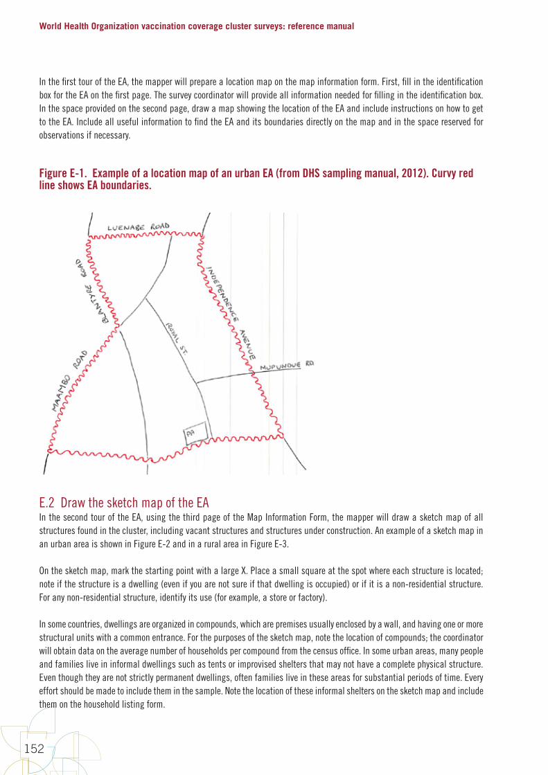
World Health Organization vaccination coverage cluster surveys: reference manual
152
In the first tour of the EA, the mapper will prepare a location map on the map information form. First, fill in the identification box for the EA on the first page. The survey coordinator will provide all information needed for filling in the identification box. In the space provided on the second page, draw a map showing the location of the EA and include instructions on how to get to the EA. Include all useful information to find the EA and its boundaries directly on the map and in the space reserved for observations if necessary.
Figure E-1. Example of a location map of an urban EA (from DHS sampling manual, 2012). Curvy red line shows EA boundaries.
E.2 Draw the sketch map of the EAIn the second tour of the EA, using the third page of the Map Information Form, the mapper will draw a sketch map of all structures found in the cluster, including vacant structures and structures under construction. An example of a sketch map in an urban area is shown in Figure E-2 and in a rural area in Figure E-3.
On the sketch map, mark the starting point with a large X. Place a small square at the spot where each structure is located; note if the structure is a dwelling (even if you are not sure if that dwelling is occupied) or if it is a non-residential structure. For any non-residential structure, identify its use (for example, a store or factory).
In some countries, dwellings are organized in compounds, which are premises usually enclosed by a wall, and having one or more structural units with a common entrance. For the purposes of the sketch map, note the location of compounds; the coordinator will obtain data on the average number of households per compound from the census office. In some urban areas, many people and families live in informal dwellings such as tents or improvised shelters that may not have a complete physical structure. Even though they are not strictly permanent dwellings, often families live in these areas for substantial periods of time. Every effort should be made to include them in the sample. Note the location of these informal shelters on the sketch map and include them on the household listing form.
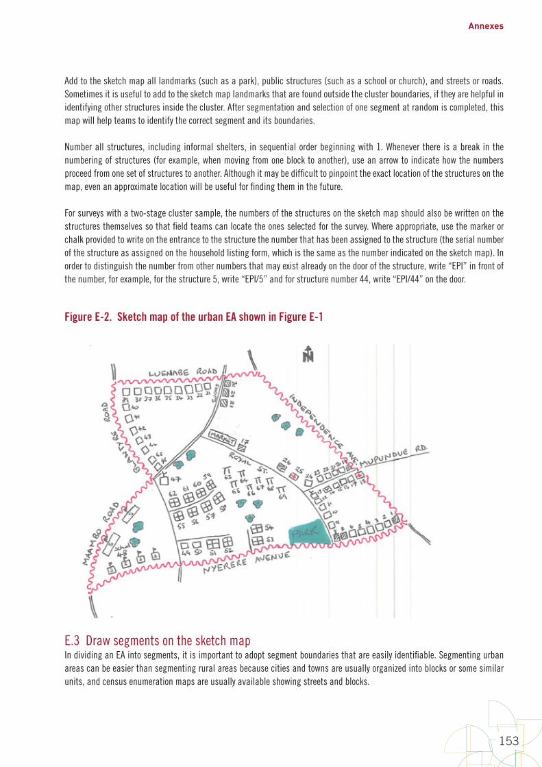
Annexes
153
Add to the sketch map all landmarks (such as a park), public structures (such as a school or church), and streets or roads. Sometimes it is useful to add to the sketch map landmarks that are found outside the cluster boundaries, if they are helpful in identifying other structures inside the cluster. After segmentation and selection of one segment at random is completed, this map will help teams to identify the correct segment and its boundaries.
Number all structures, including informal shelters, in sequential order beginning with 1. Whenever there is a break in the numbering of structures (for example, when moving from one block to another), use an arrow to indicate how the numbers proceed from one set of structures to another. Although it may be difficult to pinpoint the exact location of the structures on the map, even an approximate location will be useful for finding them in the future.
For surveys with a two-stage cluster sample, the numbers of the structures on the sketch map should also be written on the structures themselves so that field teams can locate the ones selected for the survey. Where appropriate, use the marker or chalk provided to write on the entrance to the structure the number that has been assigned to the structure (the serial number of the structure as assigned on the household listing form, which is the same as the number indicated on the sketch map). In order to distinguish the number from other numbers that may exist already on the door of the structure, write “EPI” in front of the number, for example, for the structure 5, write “EPI/5” and for structure number 44, write “EPI/44” on the door.
Figure E-2. Sketch map of the urban EA shown in Figure E-1
E.3 Draw segments on the sketch mapIn dividing an EA into segments, it is important to adopt segment boundaries that are easily identifiable. Segmenting urban areas can be easier than segmenting rural areas because cities and towns are usually organized into blocks or some similar units, and census enumeration maps are usually available showing streets and blocks.
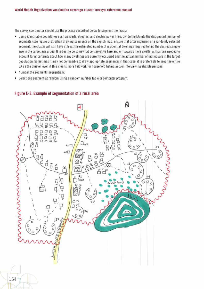
World Health Organization vaccination coverage cluster surveys: reference manual
154
The survey coordinator should use the process described below to segment the maps:
• Using identifiable boundaries such as roads, streams, and electric power lines, divide the EA into the designated number of segments (see Figure E-3). When drawing segments on the sketch map, ensure that after exclusion of a randomly selected segment, the cluster will still have at least the estimated number of residential dwellings required to find the desired sample size in the target age group. It is best to be somewhat conservative here and err towards more dwellings than are needed to account for uncertainty about how many dwellings are currently occupied and the actual number of individuals in the target population. Sometimes it may not be feasible to draw appropriate segments; in that case, it is preferable to keep the entire EA as the cluster, even if this means more fieldwork for household listing and/or interviewing eligible persons.
• Number the segments sequentially.
• Select one segment at random using a random number table or computer program.
Figure E-3. Example of segmentation of a rural area
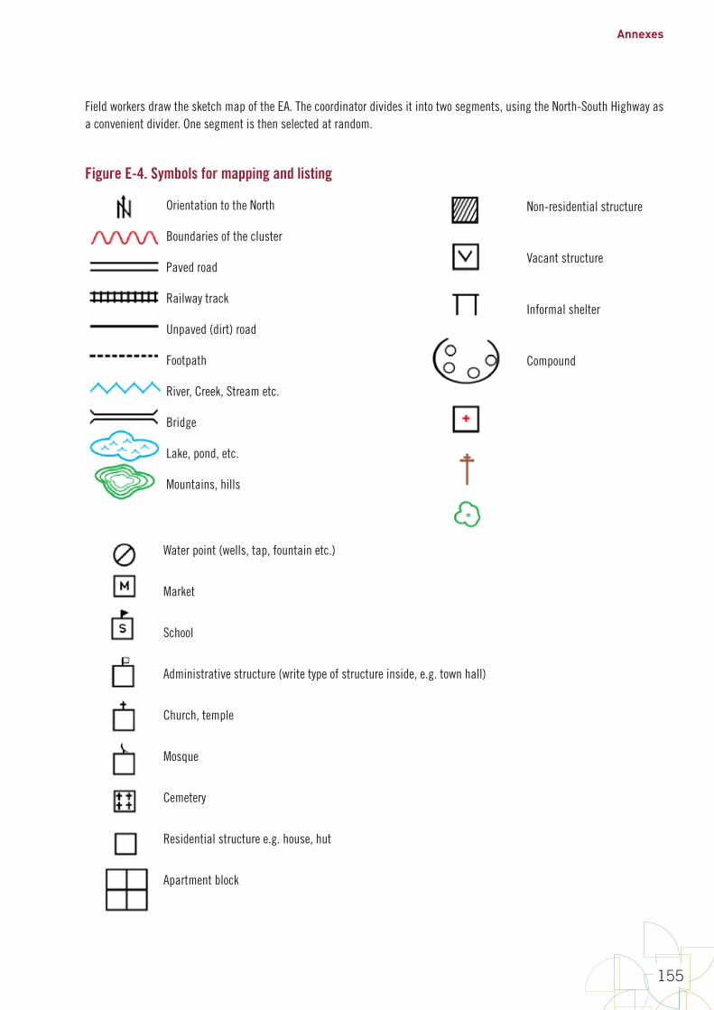
Annexes
155
Field workers draw the sketch map of the EA. The coordinator divides it into two segments, using the North-South Highway as a convenient divider. One segment is then selected at random.
Figure E-4. Symbols for mapping and listing
Orientation to the North
Boundaries of the cluster
Paved road
Railway track
Unpaved (dirt) road
Footpath
River, Creek, Stream etc.
Bridge
Lake, pond, etc.
Mountains, hills
Water point (wells, tap, fountain etc.)
Market
School
Administrative structure (write type of structure inside, e.g. town hall)
Church, temple
Mosque
Cemetery
Residential structure e.g. house, hut
Apartment block
Non-residential structure
Vacant structure
Informal shelter
Compound

World Health Organization vaccination coverage cluster surveys: reference manual
156
Annex F: How to enumerate and select households in a two-stage cluster sample
For surveys of routine vaccination coverage of children aged 12–23 months, it will often be efficient to do a single-stage cluster sample and enrol all eligible children in the selected clusters or segments.
For surveys of wider target age groups, or for those with very long questionnaires, a two-stage sample is a good option. In a two-stage sample, household listing is done first, followed by random selection of households for the completion of individual questionnaires.
The household listing operation consists of visiting each of the selected clusters, collecting geographic coordinates of the cluster, drawing a location map and sketch map as shown in annex E, and recording on listing forms a description of every dwelling together with the names of the heads of the households in the dwellings. Mapping and listing of households represents a substantial field cost, but it is essential to guarantee the exactness of sample implementation.
F.1 DefinitionsA structure is a free-standing building or other construction that can have one or more dwelling units for residential or commercial use. Residential structures can have one or more dwelling units (for example, single house, apartment structure, compound, etc). A structure is called a multi-unit structure if it contains more than one household in the structure. Otherwise it is called a single-unit structure.
A dwelling unit is a room or a group of rooms normally intended as a residence for one household (for example: a single house, an apartment, a group of rooms in a house); a dwelling unit can also have more than one household.
An informal shelter is a non-permanent structure such as a tent, or semi-covered living area, where persons sleep regularly. It is most commonly found in urban areas having large homeless populations. It is usually not possible to capture all homeless populations in a survey, but when there are areas known to be used regularly and to have informal shelters, efforts should be made to include them in the household listing operation.
A household consists of a person or a group of related or unrelated persons, who live together in the same dwelling unit or informal shelter, who acknowledge one adult male or female 15 years old or older as the head of the household, who share the same housekeeping arrangements, and are considered as one unit. In some cases one may find a group of people living together in the same house, but each person has separate eating arrangements; they should be counted as separate one-person households. Collective living arrangements such as army camps, boarding schools or prisons should not be considered as households. Examples of households are:
• a man with his wife or his wives, with or without children
• a man with his wife or his wives, his children and his parents
• a man with his wife or his wives, his married children living together for social or economic reasons (the group recognize one person as household head)
• a widowed, divorced or separated man or woman with or without children
• a single mother and her children.
The head of household is the person who is acknowledged as such by members of the household and who is usually responsible for the upkeep and maintenance of the household.

Annexes
157
A location map is a map produced in the household listing operation that indicates the main access to a cluster, including main roads and main landmarks in the cluster, and sometimes includes important landmarks in the neighbouring cluster.
A sketch map is a map showing the location or marks of all structures found in the listing operation that helps the interviewer to locate the selected households. A sketch map also contains the cluster identification information, location information, access information, principal physical features and landmarks such as mountains, rivers, roads and electric poles.
F.2 Responsibilities of the listing staffPersons recruited to participate in the household listing operation will work in teams consisting of two enumerators. A coordinator will monitor the entire operation.
The responsibilities of the coordinator are to:
• obtain base maps for all the clusters included in the survey
• arrange for the reproduction of all listing materials (listing manuals, mapping and listing forms) –the map information forms and the household listing forms must be prepared in sufficient numbers to cover all of the clusters to be visited
• assign teams to clusters
• monitor the reception of the completed listing forms at the central office
• verify that the quality of work is acceptable.
If GPS coordinates are being collected during the listing operation, the coordinator must also:
• obtain one GPS receiver per listing team, plus two backup receivers, and tag each GPS receiver with a number
• ensure that all GPS receivers have the correct settings and distribute a receiver to each field team
• obtain and copy all GPS training materials for listing staff
• train all listing staff to record GPS waypoints in the GPS units and record them on the paper form.
The responsibilities of the enumerators are to:
• identify the boundaries of the cluster
• draw a location map showing the location of the clustdraw a detailed sketch map of the cluster showing the locations of all structures residing in the cluster
• list all the households in the cluster in a systematic manner
• communicate to the coordinator problems encountered in the field and follow his/her instructions
• transfer the completed listing forms to the coordinator or to the central office.
If GPS coordinates are being collected during the listing operation, enumerators must also capture and record the GPS waypoint of the centre of the cluster, the cluster boundaries and each structure in the cluster.
The materials needed for the household listing operation are:
1. manual for household listing
2. base map of the area containing the cluster
3. Map Information Form
4. Household Listing Form.

World Health Organization vaccination coverage cluster surveys: reference manual
158
If GPS coordinates are to be recorded during the listing operation and are not recorded automatically by the equipment used for data capture, the following additional materials are needed:
1. GPS receivers, batteries and cables
2. GPS training manuals and handouts.
F.3 Locating the cluster and drawing maps This is done as described in Annex E.
F.4 Listing of householdsThe lister will use the Household Listing Form to record all households found in the cluster. Annex H lists data elements to include when designing a household listing form. The text in this section describes some work using the form DHS/2 which is depicted on the last page of this Annex. Your form may vary slightly from this one, but should include the important data elements listed here and in Annex H.
A structure is called a multi-unit structure if it contains more than one household in the structure; otherwise it is called a single-unit structure. All households found in a structure or multi-unit structure must be numbered from 1 to m, within the structure1. The structure number plus the household number form a unique identification number for each household in the cluster. For example, household number 3 in structure number 44 would be uniquely identified with ID number 44-3.
It is useful to write the household ID number at the entrance of the household to later assist the interviewer to identify the household for interview in two-stage samples, and for repeat visits and quality control in both single- or two-stage samples.
Begin by entering the identification information for the cluster. The first two columns are reserved for office use only—leave them blank.
Complete the rest of the form as follows:
1. Column (1) [Serial Number of Structure]: For each structure, record the same structure serial number that the mapper enters on the sketch map. All the structures recorded on the sketch map (except the landmarks) must be recorded on the listing form and numbered.
2. Column (2) [Address/Description of Structure]: Record the street address of the structure. Where structures do not have visible street addresses (especially in rural areas), give a description of the structure and any details that help in locating it (for example, in front of the school, next to the store, etc.). Note that this is not essential in single-stage cluster surveys because interviews are completed concurrently, however it is recommended because it will be helpful if revisits are needed to complete any interviews, and for revisits done by supervisors or coordinators for quality control.
3. Column (3) [Residence Y/N]: Indicate whether the structure is used for residential purposes (eating and sleeping) by writing Y for “Yes”. In cases where a structure is used for commercial or other purposes, write N for “No”. Structures used both for residential and commercial purposes (for example, a combination of store and home) should be classified as residential, and marked Y in column 3). Make sure to list any household unit found in a non-residential structure (for example, a guard living inside a factory or in a church). List any informal shelters identified. Also, do not forget to list vacant structures and structures under construction, and in Column (6) give some explanation (for example, vacant, under construction). All structures seen in the cluster should be recorded on the sketch map of the cluster and in the listing.
4. Column (4) [Serial Number of Household in Structure]: This is the serial number assigned to each household found in the structure; there can be more than one household in a structure. The first household in the structure will always have number 1.
1 This number is different from the household number later given to all of the households listed in the whole cluster just prior to household selection.
Annexes
159
If there is a second household in the structure, this household should be recorded on the next line with a 2 recorded in Column (4); Columns (1) to (3) repeat the structure number and address or are left blank.
5. Column (5) [Name of Head of Household]: Write the name of the head of the household. There can only be one head per household. If no one is home or the household refuses to cooperate, ask neighbours for the name of the head of the household. If a name cannot be determined, leave this column blank. It is not the name of the landlord or owner of the structure that is needed, but the name of the head of the household who lives there.
6. Column (6) [Observations/Occupied or not]: This space is provided for any special remarks that might help the coordinator decide whether to include a household in the household selection, and might also help the interviewing team locate the structure or identify the household during the main survey fieldwork.
If the structure is an apartment block or block of flats or apartments, assign one serial number to the entire structure (only one square with one number appears on the sketch map), but complete Columns (2) through (6) for each apartment in the structure individually. Each apartment should have its own address, which is the apartment number within the structure. The same process is done for compounds in rural areas.
The listing team should be careful to locate hidden structures. In some areas, structures may have been built so haphazardly that they are easily missed. In rural areas, structures may be hidden by tall grasses and trees. If there is a pathway leading from the listed structure, check to see if the pathway goes to another structure. Talking with people living in the area may help with identifying hidden structures.
F.5 Quality controlQuality checks should be performed to ensure that the work done by each listing team is acceptable. The coordinator should tour the regions during the household listing operation, and assess the quality of the finished clusters. The coordinator should select a finished cluster and do an independent listing of 10% of the cluster. If important errors are found, the whole cluster should be relisted. If the problem is related to systematic errors and it is not possible to do corrections on the listing forms, then all of the listed clusters should be relisted.
F.6 Prepare the household listing forms for household selectionHousehold selection might be done by staff in a Central Office, after the household listing forms are turned in, or in some cases the selection might be accomplished in the field, possibly on the same data that interviews are scheduled to begin.
Once the central office receives the completed listing materials for a cluster, they first assign a serial number to all of the households in the cluster in the second column of the form DHS/2. An example is provided on the last page of this Annex.
Only occupied residential households (including households that refused to cooperate at the time of listing and households where the occupants were absent at the time of listing but would return shortly and would be at home during the period of household interview) will be numbered.
• This is a new continuous serial number from 1 to the total number of occupied residential households listed in the cluster.
• Leave the cell in the second column blank if the household is not occupied, or if the structure is not a residential structure.
• Fill in the second column only if the structure on that row is an occupied household.
• Make sure that the numbering of all occupied households follows sequentially from the previous occupied household on the list, with no gaps or repetitions in the numbering.

World Health Organization vaccination coverage cluster surveys: reference manual
160
F.7 Instructions for having staff in a central office select the householdsAfter assigning the serial numbers to all households listed in the cluster, the central office staff will use a protocol for randomly selecting the right number of households. This process will likely involve a table of random numbers or a computer spreadsheet or program to identify a random subset of household serial numbers. The process should be specified in the survey protocol and documented carefully.
The Internet has numerous web pages with instructions for using a spreadsheet to identify a random sample. One simple process using Microsoft Excel is as follows:
1. Enter the serial numbers of eligible households in column A of a new spreadsheet. (1 in the first row, 2 in the second row, etc.)
2. Enter the formula =RAND() in column B of the spreadsheet beside each household’s serial number. This will yield a random number between 0 and 1 in column B.
3. Click at the top of the column to select Column B. Click ‘copy’ and click ‘Paste->Values’ to replace the formula with the random numbers (so the formula does not change the numbers later.)
4. Sort the entire spreadsheet (columns A and B together) based on the numbers in column B (lowest-to-highest). This will re-order the household serial numbers in a random fashion.
5. The households listed at the top of the spreadsheet are those selected for the survey. If the protocol indicates that staff should visit 12 households in each cluster, then record the serial numbers of the top 12 cells of column A. Save the spreadsheet to document the selection.
When the central office produces the list of selected households, they can be marked carefully on the household listing form. Copy the numbers of the selected households to the first column of the form DHS/2, corresponding to the serial number of the households in the listing form. These are the households that must be interviewed. It is recommended to use a different coloured pen on the listing forms to indicate the households selected for interviewing. It is also very helpful to use colour on the cluster’s sketch map to mark the structures where the selected households are located.
F.8 Instructions for household selection by staff in the fieldWhen the household listing occurs on the same day that interviews are scheduled to start, it may not be possible to have the household selection accomplished at a central office, though this is the preferred approach. Make every effort to have a central office do the selection to be sure to avoid any temptation that can bias the work in the field. If the selection must be done by field staff, then have the central office prepare a list of randomly-ordered numbers between 1 and something high like 500. Print the numbers in randomly selected order and seal the pages in an envelope that can be sent to the field. After households are listed and serial numbers are assigned, open the envelope and read the numbers down the list. The first number from the envelope is the serial number of the first household selected in to the sample. The second number from the envelope is the serial number of the second household selected in to the sample. And so on. It is important that the sheets in the envelope have numbers that go up at least as high as the number of eligible homes in the cluster, so it may be necessary for the central office staff to always print lists that include numbers up to 250 or 500 or whatever figure will be sure to be high enough. Staff can identify the randomly selected households using the lists from the envelope. The sheets from the envelope should be saved and turned in with the other forms from the cluster, to document how households were identified.
Another alternative for selecting a random list of households while in the field is to use a handheld computer or smartphone application. There are programs that allow a team to walk around the cluster, listing households in one step, noting whether respondents are eligible or not, and recording a serial number for each household along with its GPS coordinates. Then in a later step the application can select a random subset from the list and provide the team with a list of serial numbers of selected households, along with GPS coordinates to help field staff go back and conduct interviews in those households.
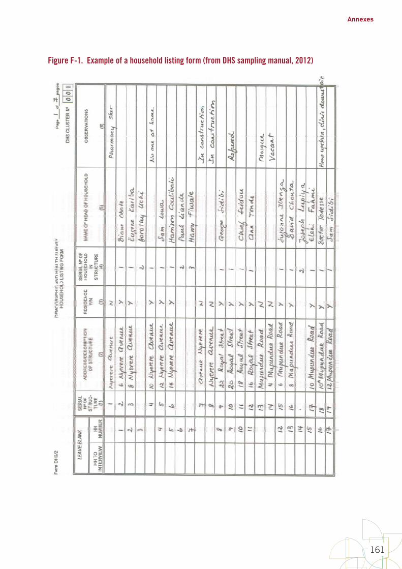
Annexes
161
Figure F-1. Example of a household listing form (from DHS sampling manual, 2012)
F-8
Figure F-1. Example of a household listing form (from DHS sampling manual, 2012)

World Health Organization vaccination coverage cluster surveys: reference manual
162
Annex G: Tips for high-quality training of survey staff
For any vaccination coverage survey, it is essential that the staff be qualified and well trained. Interviewers must be able follow the protocol for identifying the appropriate households, establishing who in the household is eligible, conducting the interview, and completely and correctly recording the information on the survey forms. The text below only provides guidance on training for survey interviewers as an example. Training is also needed for personnel doing household listing and for supervisors.
G.1 Training topicsIn some cases, the purpose of the training is to improve the team members’ understanding of the objectives and methods of the survey. In other instances, the purpose is to ensure that team members correctly perform a task. Where performance of a task is required it is important that the staff not only understand what to do but that they have an opportunity to practice the task with both common and easily understood examples as well as more difficult ones.
During training it is important to ensure that participants have appropriate information on the objectives of the survey and what their roles will be. They should be aware of the different vaccine-preventable diseases for which the vaccine programme provides vaccines, what the different vaccine names are, how many does are required and how they are administered. They should also know what the target populations (for example, women of childbearing age, girls 9–14 years of age, infants less than one year of age, all children under five years of age).
Information from the interview must be clearly and completely records on the survey data collection tools. The tools should be designed such that there is adequate space for the interviewer to easily record the replies. It is usually useful that half an hour or so be spent on practicing recording letters and digits on the form in a standardized way. Handwriting exercises often done by young children are useful and should be used during the training. Such exercises and worksheets are readily available on the Internet and can be adapted as necessary.
Several topics in vaccination surveys are important to learn but difficult to convey. Two of the most important are the issue of eligibility and how to interpret evidence of vaccination.
Survey eligibility
In most vaccination coverage surveys, whether questions are asked about an individual's vaccination history will depend on the individual's age. The eligibility criteria might also include residential status, sex, or other factors. Training on how to ascertain whether the individual should be included in the survey is essential. It may be helpful to build survey aids such as calendars of local events, age estimation charts or pre-calculated eligible dates of birth.
Evidence of vaccination
To complete the survey forms, staff should be familiar with the kinds of evidence used to establish vaccination status. This includes both home-based vaccination or child health cards as well as records kept in health facilities. It might also include records given during supplemental immunization activities (SIAs) and physical marks for vaccinated individuals such as fingernail colouring. The evidence of vaccination from these sources may require interpretation before being recorded on the survey data collection forms and it is essential that interviewers and supervisors can accurately record the vaccination status documented by the different sources of data.

Annexes
163
The naming of vaccines may not be consistent over time, from place to place and source of vaccination. For example, a common name for the diphtheria-pertussis-tetanus-HepB-Hib pentavalent vaccine is “penta”. In some instances the pentavalent vaccine may have recently been introduced and the cards used may still use the name DPT or DTP. The training should include a detailed presentation with examples of the different types of cards that might be seen in the survey and how this information should be recorded.
In some instances children have been vaccinated and no record or physical evidence of that vaccination is available, and the only evidence of the child's vaccination status is that of the child's caretaker's memory. Eliciting as much detail as possible regarding the child's vaccination history from the caretaker is likely to improve the accuracy of their report. It is essential that the training include the appropriate way to gather data based on both documented records and caretaker recall.
G.2 Training methodsOne of the most valuable methods for learning a new task is role playing. Short scenarios should be developed and presented (with team members participating) to the group. It is useful if scenarios not only present correct examples but also include errors for the group to find. The scenarios are useful to identify any lack of complete and common understanding, and surface these issues for group discussion. Such scenarios could include household identification, introduction to the household, eligibility issues and other tasks. Recording and showing short videos of field practice is also useful.
Presentations, examples, practice sessions and role playing scenarios should be prepared prior to the training session. If time permits, training session participants can also practice tasks (for example, conducting an interview) and role playing (determining how may in the house are eligible for the survey) with other participants. Many surveys prepare a manual or standard operating procedures (SOP) for the interviewers and supervisors. The manual should be reviewed during the training. In addition, participants should be encouraged to refer to the manual during exercises, practice sessions and role playing.
G.3 Training scheduleTraining for interviewers and supervisors requires approximately five days, including at least one day in the community practicing the protocol and instruction on the following topics: identifying the appropriate households, obtaining permission to conduct the interview, selecting eligible individuals in the household, using the survey tools to conduct the interview, obtaining the appropriate responses, and clearly and accurately recording the responses.
Below is a sample agenda for a five-day training session for interviewers and field supervisors. The training may take more time if GPS systems, digital recording or cameras are used. It is important that the interviewers and supervisors understand the equipment, how it is to be used and to have time to practice its use.
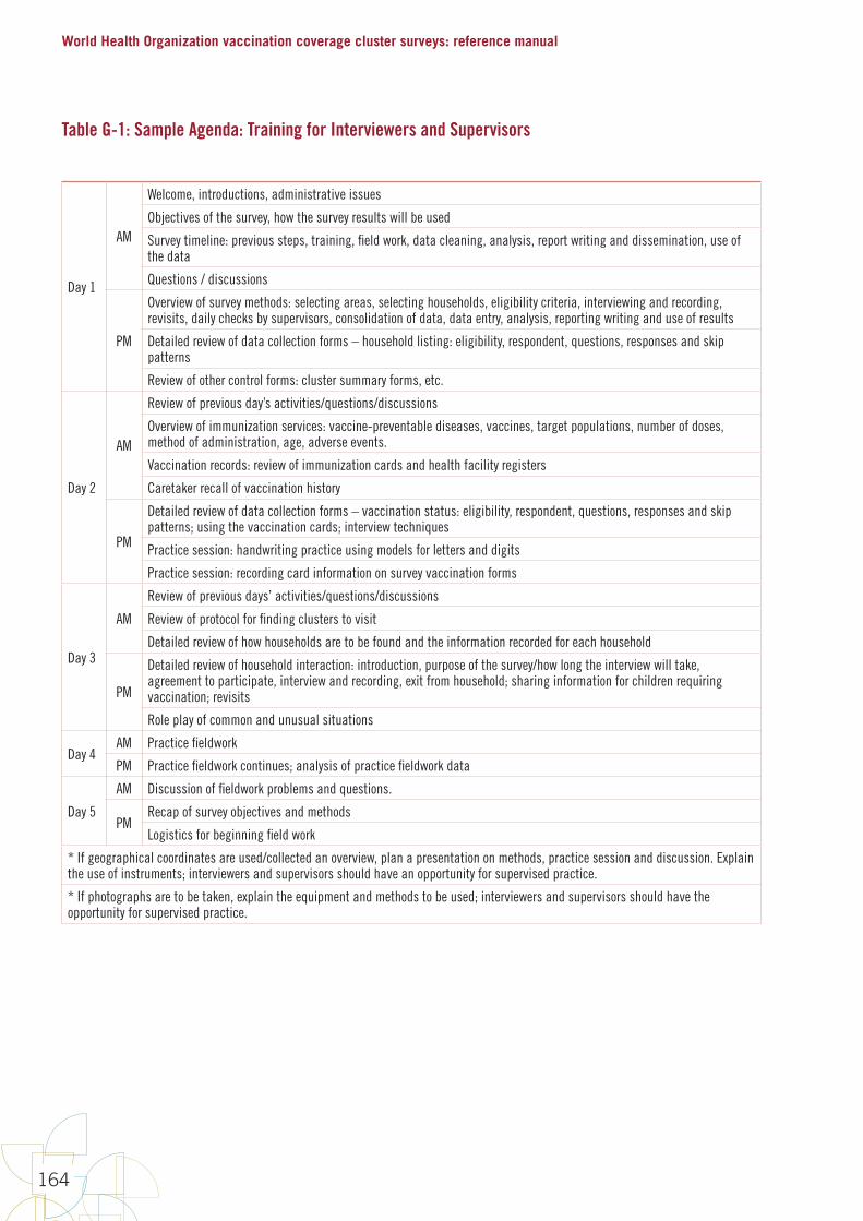
World Health Organization vaccination coverage cluster surveys: reference manual
164
Table G-1: Sample Agenda: Training for Interviewers and Supervisors
Day 1
AM
Welcome, introductions, administrative issues
Objectives of the survey, how the survey results will be used
Survey timeline: previous steps, training, field work, data cleaning, analysis, report writing and dissemination, use of the data
Questions / discussions
PM
Overview of survey methods: selecting areas, selecting households, eligibility criteria, interviewing and recording, revisits, daily checks by supervisors, consolidation of data, data entry, analysis, reporting writing and use of results
Detailed review of data collection forms – household listing: eligibility, respondent, questions, responses and skip patterns
Review of other control forms: cluster summary forms, etc.
Day 2
AM
Review of previous day’s activities/questions/discussions
Overview of immunization services: vaccine-preventable diseases, vaccines, target populations, number of doses, method of administration, age, adverse events.
Vaccination records: review of immunization cards and health facility registers
Caretaker recall of vaccination history
PM
Detailed review of data collection forms – vaccination status: eligibility, respondent, questions, responses and skip patterns; using the vaccination cards; interview techniques
Practice session: handwriting practice using models for letters and digits
Practice session: recording card information on survey vaccination forms
Day 3
AM
Review of previous days’ activities/questions/discussions
Review of protocol for finding clusters to visit
Detailed review of how households are to be found and the information recorded for each household
PM
Detailed review of household interaction: introduction, purpose of the survey/how long the interview will take, agreement to participate, interview and recording, exit from household; sharing information for children requiring vaccination; revisits
Role play of common and unusual situations
Day 4AM Practice fieldwork
PM Practice fieldwork continues; analysis of practice fieldwork data
Day 5
AM Discussion of fieldwork problems and questions.
PMRecap of survey objectives and methods
Logistics for beginning field work
* If geographical coordinates are used/collected an overview, plan a presentation on methods, practice session and discussion. Explain the use of instruments; interviewers and supervisors should have an opportunity for supervised practice.
* If photographs are to be taken, explain the equipment and methods to be used; interviewers and supervisors should have the opportunity for supervised practice.

Annexes
165
Annex H: Sample survey questions
This annex provides lists of questions and guidance on what type of responses and skip patterns might be appropriate. Sample questionnaires are available at the WHO page on vaccination coverage surveys: http://www.who.int/immunization/monitoring_surveillance/routine/coverage/en/index2.html. Data that use these variable names and response codes are compatible with the Vaccination Coverage Quality Indicators (VCQI) tool. Each form is divided into three sections: a suggested header with information for field staff to fill in before they begin the data collection, the main body of the form, and a footer with information for staff to fill in when they finish the work.
The header always includes several fields to identify which stratum and cluster the data is being collected from. If possible, these fields should either be pre-printed on the forms, or pre-printed on weather-proof stickers to be applied to the forms, so that stratum ID and cluster ID will be correct, easy to for data entry clerks to read, and recorded in a uniform fashion across the entire survey.
The main body of the form includes items that will be repeated many times with one entry per household or one entry per respondent. Paper forms should be laid out in a manner that provides enough room to fill in each entry, so it may work best to use two or three rows per entry on the form, instead of one small cramped row. In some cases it may be appropriate to use a separate paper form for each respondent. In other cases you may design forms that will accommodate responses from several respondents on one sheet of paper.
The footer includes fields to document when the work in the household or cluster is finished and spaces for comments so field staff can note information that may be helpful later in interpreting the survey data. On paper forms, be sure to leave large spaces for clearly written comments, including text on how the interview went. Be sure to have data entry clerks enter those comments into the database so they are available to analysts later.
Note that this annex does not include many demographic questions about the respondents’ wealth, education, urban/rural status, occupation or religion. If your survey steering committee wishes to disaggregate results by demographic categories, you will need to add questions to the survey to collect those data elements.
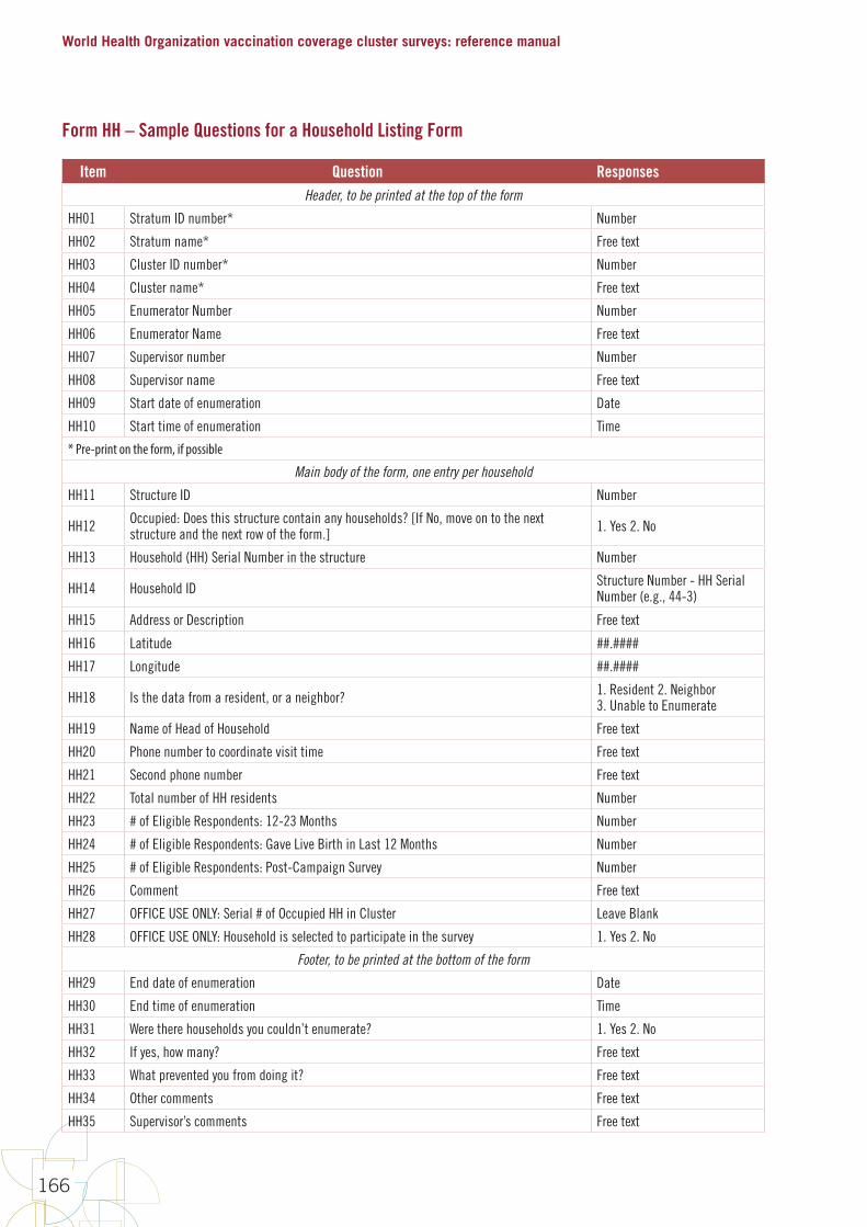
World Health Organization vaccination coverage cluster surveys: reference manual
166
Form HH – Sample Questions for a Household Listing Form
Item Question ResponsesHeader, to be printed at the top of the form
HH01 Stratum ID number* Number
HH02 Stratum name* Free text
HH03 Cluster ID number* Number
HH04 Cluster name* Free text
HH05 Enumerator Number Number
HH06 Enumerator Name Free text
HH07 Supervisor number Number
HH08 Supervisor name Free text
HH09 Start date of enumeration Date
HH10 Start time of enumeration Time
* Pre-print on the form, if possible
Main body of the form, one entry per household
HH11 Structure ID Number
HH12 Occupied: Does this structure contain any households? [If No, move on to the next structure and the next row of the form.] 1. Yes 2. No
HH13 Household (HH) Serial Number in the structure Number
HH14 Household ID Structure Number - HH Serial Number (e.g., 44-3)
HH15 Address or Description Free text
HH16 Latitude ##.####
HH17 Longitude ##.####
HH18 Is the data from a resident, or a neighbor? 1. Resident 2. Neighbor3. Unable to Enumerate
HH19 Name of Head of Household Free text
HH20 Phone number to coordinate visit time Free text
HH21 Second phone number Free text
HH22 Total number of HH residents Number
HH23 # of Eligible Respondents: 12-23 Months Number
HH24 # of Eligible Respondents: Gave Live Birth in Last 12 Months Number
HH25 # of Eligible Respondents: Post-Campaign Survey Number
HH26 Comment Free text
HH27 OFFICE USE ONLY: Serial # of Occupied HH in Cluster Leave Blank
HH28 OFFICE USE ONLY: Household is selected to participate in the survey 1. Yes 2. No
Footer, to be printed at the bottom of the form
HH29 End date of enumeration Date
HH30 End time of enumeration Time
HH31 Were there households you couldn’t enumerate? 1. Yes 2. No
HH32 If yes, how many? Free text
HH33 What prevented you from doing it? Free text
HH34 Other comments Free text
HH35 Supervisor’s comments Free text
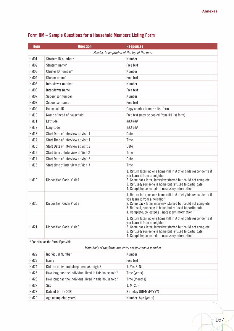
Annexes
167
Form HM – Sample Questions for a Household Members Listing Form
Item Question ResponsesHeader, to be printed at the top of the form
HM01 Stratum ID number* Number
HM02 Stratum name* Free text
HM03 Cluster ID number* Number
HM04 Cluster name* Free text
HM05 Interviewer number Number
HM06 Interviewer name Free text
HM07 Supervisor number Number
HM08 Supervisor name Free text
HM09 Household ID Copy number from HH list form
HM10 Name of head of household Free text (may be copied from HH list form)
HM11 Latitude ##.####
HM12 Longitude ##.####
HM13 Start Date of Interview at Visit 1 Date
HM14 Start Time of Interview at Visit 1 Time
HM15 Start Date of Interview at Visit 2 Date
HM16 Start time of Interview at Visit 2 Time
HM17 Start Date of Interview at Visit 3 Date
HM18 Start time of Interview at Visit 3 Time
HM19 Disposition Code: Visit 1
1. Return later; no one home (fill in # of eligible respondents if you learn it from a neighbor)2. Come back later; interview started but could not complete 3. Refused; someone is home but refused to participate4. Complete; collected all necessary information
HM20 Disposition Code: Visit 2
1. Return later; no one home (fill in # of eligible respondents if you learn it from a neighbor)2. Come back later; interview started but could not complete 3. Refused; someone is home but refused to participate4. Complete; collected all necessary information
HM21 Disposition Code: Visit 3
1. Return later; no one home (fill in # of eligible respondents if you learn it from a neighbor)2. Come back later; interview started but could not complete 3. Refused; someone is home but refused to participate4. Complete; collected all necessary information
* Pre-print on the form, if possible
Main body of the form, one entry per household member
HM22 Individual Number Number
HM23 Name Free text
HM24 Did the individual sleep here last night? 1. Yes 2. No
HM25 How long has the individual lived in this household? Time (years)
HM26 How long has the individual lived in this household? Time (months)
HM27 Sex 1. M 2. F
HM28 Date of birth (DOB) Birthday (DD/MM/YYYY)
HM29 Age (completed years) Number: Age (years)
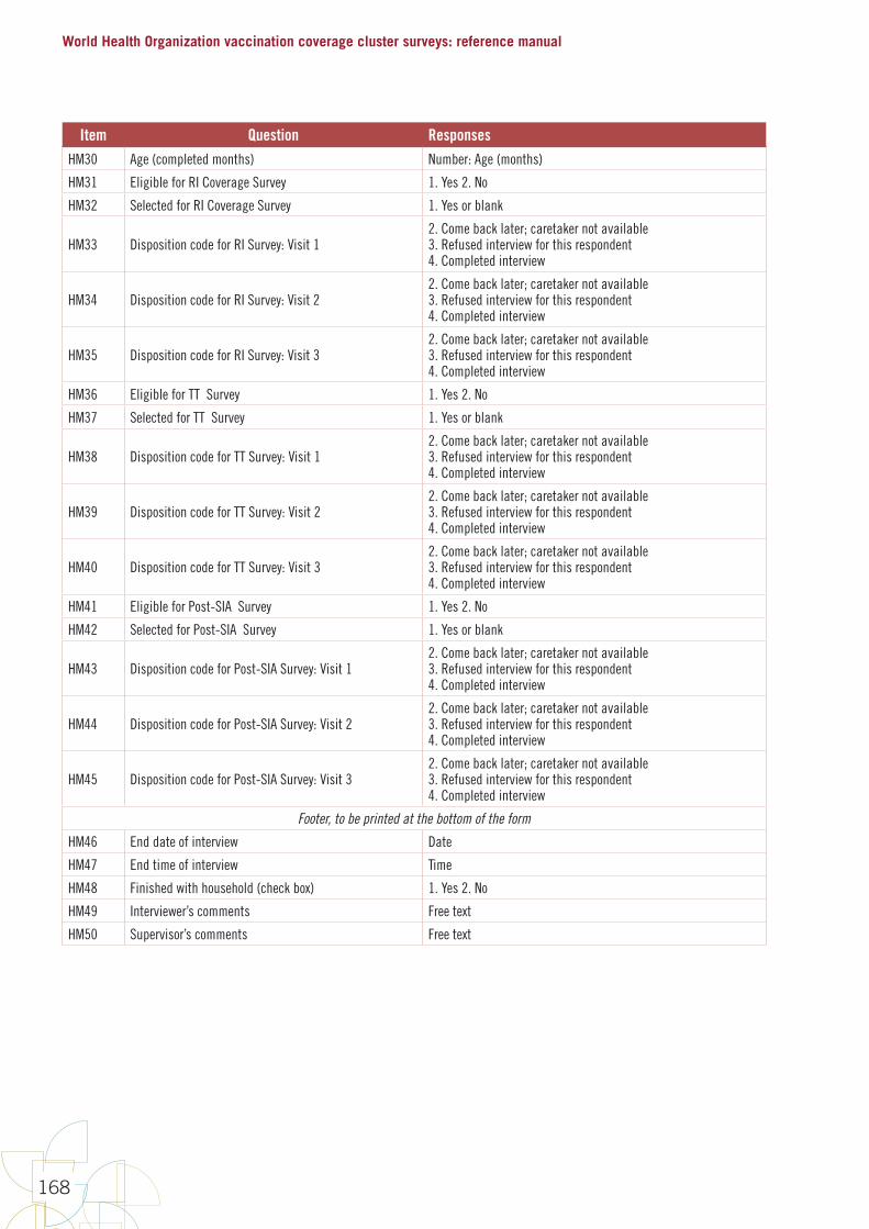
World Health Organization vaccination coverage cluster surveys: reference manual
168
Item Question ResponsesHM30 Age (completed months) Number: Age (months)
HM31 Eligible for RI Coverage Survey 1. Yes 2. No
HM32 Selected for RI Coverage Survey 1. Yes or blank
HM33 Disposition code for RI Survey: Visit 12. Come back later; caretaker not available3. Refused interview for this respondent 4. Completed interview
HM34 Disposition code for RI Survey: Visit 22. Come back later; caretaker not available3. Refused interview for this respondent 4. Completed interview
HM35 Disposition code for RI Survey: Visit 32. Come back later; caretaker not available3. Refused interview for this respondent 4. Completed interview
HM36 Eligible for TT Survey 1. Yes 2. No
HM37 Selected for TT Survey 1. Yes or blank
HM38 Disposition code for TT Survey: Visit 12. Come back later; caretaker not available3. Refused interview for this respondent 4. Completed interview
HM39 Disposition code for TT Survey: Visit 22. Come back later; caretaker not available3. Refused interview for this respondent 4. Completed interview
HM40 Disposition code for TT Survey: Visit 32. Come back later; caretaker not available3. Refused interview for this respondent 4. Completed interview
HM41 Eligible for Post-SIA Survey 1. Yes 2. No
HM42 Selected for Post-SIA Survey 1. Yes or blank
HM43 Disposition code for Post-SIA Survey: Visit 12. Come back later; caretaker not available3. Refused interview for this respondent 4. Completed interview
HM44 Disposition code for Post-SIA Survey: Visit 22. Come back later; caretaker not available3. Refused interview for this respondent 4. Completed interview
HM45 Disposition code for Post-SIA Survey: Visit 32. Come back later; caretaker not available3. Refused interview for this respondent 4. Completed interview
Footer, to be printed at the bottom of the form
HM46 End date of interview Date
HM47 End time of interview Time
HM48 Finished with household (check box) 1. Yes 2. No
HM49 Interviewer’s comments Free text
HM50 Supervisor’s comments Free text
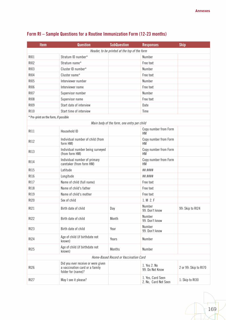
Annexes
169
Form RI – Sample Questions for a Routine Immunization Form (12-23 months)
Item Question SubQuestion Responses Skip Header, to be printed at the top of the form
RI01 Stratum ID number* Number
RI02 Stratum name* Free text
RI03 Cluster ID number* Number
RI04 Cluster name* Free text
RI05 Interviewer number Number
RI06 Interviewer name Free text
RI07 Supervisor number Number
RI08 Supervisor name Free text
RI09 Start date of interview Date
RI10 Start time of interview Time
* Pre-print on the form, if possible
Main body of the form, one entry per child
RI11 Household ID Copy number from Form HM
RI12 Individual number of child (from form HM)
Copy number from Form HM
RI13 Individual number being surveyed (from form HM)
Copy number from Form HM
RI14 Individual number of primary caretaker (from form HM)
Copy number from Form HM
RI15 Latitude ##.####
RI16 Longitude ##.####
RI17 Name of child (full name) Free text
RI18 Name of child's father Free text
RI19 Name of child's mother Free text
RI20 Sex of child 1. M 2. F
RI21 Birth date of child Day Number99. Don't know 99: Skip to RI24
RI22 Birth date of child Month Number99. Don't know
RI23 Birth date of child Year Number99. Don't know
RI24 Age of child (if birthdate not known) Years Number
RI25 Age of child (if birthdate not known) Months Number
Home-Based Record or Vaccination Card
RI26Did you ever receive or were given a vaccination card or a family folder for (name)?
1. Yes 2. No99. Do Not Know 2 or 99: Skip to RI70
RI27 May I see it please? 1. Yes, Card Seen2. No, Card Not Seen 1: Skip to RI30
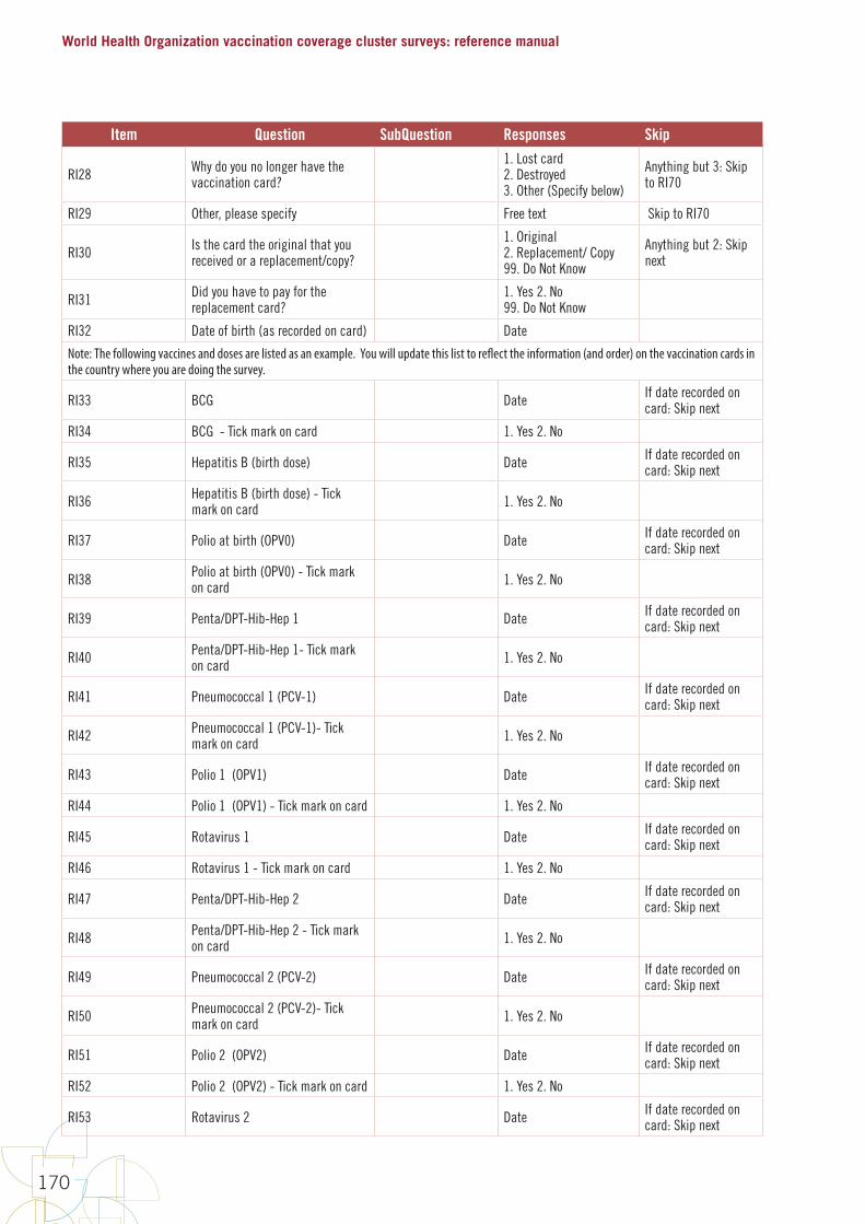
World Health Organization vaccination coverage cluster surveys: reference manual
170
Item Question SubQuestion Responses Skip
RI28 Why do you no longer have the vaccination card?
1. Lost card2. Destroyed3. Other (Specify below)
Anything but 3: Skip to RI70
RI29 Other, please specify Free text Skip to RI70
RI30 Is the card the original that you received or a replacement/copy?
1. Original2. Replacement/ Copy99. Do Not Know
Anything but 2: Skip next
RI31 Did you have to pay for the replacement card?
1. Yes 2. No99. Do Not Know
RI32 Date of birth (as recorded on card) Date
Note: The following vaccines and doses are listed as an example. You will update this list to reflect the information (and order) on the vaccination cards in the country where you are doing the survey.
RI33 BCG Date If date recorded on card: Skip next
RI34 BCG - Tick mark on card 1. Yes 2. No
RI35 Hepatitis B (birth dose) Date If date recorded on card: Skip next
RI36 Hepatitis B (birth dose) - Tick mark on card 1. Yes 2. No
RI37 Polio at birth (OPV0) Date If date recorded on card: Skip next
RI38 Polio at birth (OPV0) - Tick mark on card 1. Yes 2. No
RI39 Penta/DPT-Hib-Hep 1 Date If date recorded on card: Skip next
RI40 Penta/DPT-Hib-Hep 1- Tick mark on card 1. Yes 2. No
RI41 Pneumococcal 1 (PCV-1) Date If date recorded on card: Skip next
RI42 Pneumococcal 1 (PCV-1)- Tick mark on card 1. Yes 2. No
RI43 Polio 1 (OPV1) Date If date recorded on card: Skip next
RI44 Polio 1 (OPV1) - Tick mark on card 1. Yes 2. No
RI45 Rotavirus 1 Date If date recorded on card: Skip next
RI46 Rotavirus 1 - Tick mark on card 1. Yes 2. No
RI47 Penta/DPT-Hib-Hep 2 Date If date recorded on card: Skip next
RI48 Penta/DPT-Hib-Hep 2 - Tick mark on card 1. Yes 2. No
RI49 Pneumococcal 2 (PCV-2) Date If date recorded on card: Skip next
RI50 Pneumococcal 2 (PCV-2)- Tick mark on card 1. Yes 2. No
RI51 Polio 2 (OPV2) Date If date recorded on card: Skip next
RI52 Polio 2 (OPV2) - Tick mark on card 1. Yes 2. No
RI53 Rotavirus 2 Date If date recorded on card: Skip next

Annexes
171
Item Question SubQuestion Responses Skip RI54 Rotavirus 2- Tick mark on card 1. Yes 2. No
RI55 Penta/DPT-Hib-Hep 3 Date If date recorded on card: Skip next
RI56 Penta/DPT-Hib-Hep 3 - Tick mark on card 1. Yes 2. No
RI57 Pneumococcal 3 (PCV-3) Date If date recorded on card: Skip next
RI58 Pneumococcal 3 (PCV-3)- Tick mark on card 1. Yes 2. No
RI59 Polio 3 (OPV3) Date If date recorded on card: Skip next
RI60 Polio 3 (OPV3) - Tick mark on card 1. Yes 2. No
RI61 Rotavirus 3 Date If date recorded on card: Skip next
RI62 Rotavirus 3 - Tick mark on card 1. Yes 2. No
RI63 Polio (IPV) Date If date recorded on card: Skip next
RI64 Polio (IPV) - Tick mark on card 1. Yes 2. No
RI65 Measles (1st) Date If date recorded on card: Skip next
RI66 Measles (1st) - Tick mark on card 1. Yes 2. No
RI67 Yellow Fever Date If date recorded on card: Skip next
RI68 Yellow Fever - Tick mark on card 1. Yes 2. No
Caretaker Recall or History
Again, the vaccines and doses listed here are an example that will likely need to be updated when you design your questionnaire so the list corresponds to the vaccines delivered in your country.
RI69 Has the child received every vaccine in this survey? 1. Yes 2. No 1: Skip to RI103
RI70Has the child ever received any vaccinations, drops or injections in the past?
1. Yes 2. No99. Do Not Know 2 or 99: Skip to RI89
RI71
Has the child ever received an injection in the right upper arm or shoulder that usually causes a scar? – that is, BCG vaccination (against tuberculosis)
1. Yes 2. No99. Do Not Know 2 or 99: Skip next
RI72 If the child is present, check for evidence of a scar and record
1. Scar Present2. No Scar Present3. Child not available to check
RI73Has the child ever received any “vaccination drops in the mouth” – that is, polio?
1. Yes 2. No99. Do Not Know 2 or 99: Skip to RI76
RI74How many times was the polio vaccine received at a health facility?
Number 99. Do Not Know
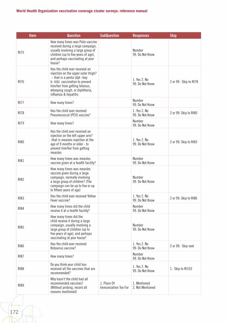
World Health Organization vaccination coverage cluster surveys: reference manual
172
Item Question SubQuestion Responses Skip
RI75
How many times was Polio vaccine received during a large campaign, usually involving a large group of children (up to five years of age), and perhaps vaccinating at your house?
Number 99. Do Not Know
RI76
Has the child ever received an injection on the upper outer thigh? – that is a penta (dpt -hep b- hib) vaccination to prevent him/her from getting tetanus, whooping cough, or diphtheria, influenza & hepatitis
1. Yes 2. No99. Do Not Know 2 or 99 : Skip to RI78
RI77 How many times? Number 99. Do Not Know
RI78 Has the child ever received Pneumococcal (PCV) vaccine?
1. Yes 2. No99. Do Not Know 2 or 99: Skip to RI80
RI79 How many times? Number 99. Do Not Know
RI80
Has the child ever received an injection on the left upper arm? -that is measles injection at the age of 9 months or older - to prevent him/her from getting measles
1. Yes 2. No99. Do Not Know 2 or 99: Skip to RI83
RI81 How many times was measles vaccine given at a health facility?
Number99. Do Not Know
RI82
How many times was measles vaccine given during a large campaign, normally involving a large group of children? (The campaign can be up to five or up to fifteen years of age)
Number99. Do Not Know
RI83 Has the child ever received Yellow Fever vaccine?
1. Yes 2. No99. Do Not Know 2 or 99: Skip to RI86
RI84 How many times did the child receive it at a health facility?
Number99. Do Not Know
RI85
How many times did the child receive it during a large campaign, usually involving a large group of children (up to five years of age), and perhaps vaccinating at your house?
Number99. Do Not Know
RI86 Has the child ever received Rotavirus vaccine?
1. Yes 2. No99. Do Not Know 2 or 99: Skip next
RI87 How many times? Number99. Do Not Know
RI88Do you think your child has received all the vaccines that are recommended?
1. Yes 2. No99. Do Not Know 1: Skip to RI103
RI89
Why hasn't the child had all recommended vaccines? (Without probing, record all reasons mentioned)
1. Place Of Immunization Too Far
1. Mentioned2. Not Mentioned

Annexes
173
Item Question SubQuestion Responses Skip
RI90 Why hasn't the child had all recommended vaccines?
2. Time Of Immunization Inconvenient
1. Mentioned2. Not Mentioned
RI91 Why hasn't the child had all recommended vaccines? 3. Mother Too Busy 1. Mentioned
2. Not Mentioned
RI92 Why hasn't the child had all recommended vaccines?
4. Family Problem, Including Illness Of Mother
1. Mentioned2. Not Mentioned
RI93 Why hasn't the child had all recommended vaccines?
5. Child Ill- Not Brought
1. Mentioned2. Not Mentioned
RI94 Why hasn't the child had all recommended vaccines?
6. Child Ill- Brought But Not Given Immunization
1. Mentioned2. Not Mentioned
RI95 Why hasn't the child had all recommended vaccines? 7. Long Wait 1. Mentioned
2. Not Mentioned
RI96 Why hasn't the child had all recommended vaccines? 8. Rumors 1. Mentioned
2. Not Mentioned
RI97 Why hasn't the child had all recommended vaccines?
9. No Faith In Immunization
1. Mentioned2. Not Mentioned
RI98 Why hasn't the child had all recommended vaccines?
10. Fear Of Side Reactions
1. Mentioned2. Not Mentioned
RI99 Why hasn't the child had all recommended vaccines?
11. Place And/Or Time Of Immunization Unknown
1. Mentioned2. Not Mentioned
RI100 Why hasn't the child had all recommended vaccines?
12. Other (Specify Below)
1. Mentioned2. Not Mentioned
RI101 Why hasn't the child had all recommended vaccines? Other, please specify Free text
RI102 Which reason above is the MOST IMPORTANT reason? 1-12
RI103 Where does your child usually receive vaccinations?
1. Local Government Health Clinic2. Local Private Doctor's Office3. Local Other 4. Outside Government Health Clinic5. Outside Private Doctor's Office6. Outside Other
RI104 Write the name of the clinic or facility. Free text
RI105
Does the child usually receive vaccinations at one of the facilities on your list? (where the team will go to search for records)
1. Yes 2. No
RI106 Where did your child receive his/her most recent vaccination?
1. Local Government Health Clinic2. Local Private Doctor's Office3. Local Other 4. Outside Government Health Clinic5. Outside Private Doctor's Office6. Outside Other

World Health Organization vaccination coverage cluster surveys: reference manual
174
Item Question SubQuestion Responses Skip
RI107Have you taken a child to a health facility for vaccination and the child was not vaccinated?
1. Yes 2. No99. Do Not Remember 2 or 99: Skip to RI118
RI108Why was the child not vaccinated?(Without probing record all reasons mentioned)
1. No Vaccine 1. Mentioned2. Not Mentioned
RI109 Why was the child not vaccinated? 2. No Vaccinator (Not Closed)
1. Mentioned2. Not Mentioned
RI110 Why was the child not vaccinated? 3. Health Facility Closed When I Went
1. Mentioned2. Not Mentioned
RI111 Why was the child not vaccinated? 4. Child Was Sick 1. Mentioned2. Not Mentioned
RI112 Why was the child not vaccinated?
5. Not Enough Children Present To Open A Vial of Vaccine
1. Mentioned2. Not Mentioned
RI113 Why was the child not vaccinated?6. The Visit Was Not On The Vaccination Day
1. Mentioned2. Not Mentioned
RI114 Why was the child not vaccinated? 7. Wait was too long 1. Mentioned2. Not Mentioned
RI115 Why was the child not vaccinated? 8. Others (Specify Below)
1. Mentioned2. Not Mentioned
RI116 Why was the child not vaccinated? 9. Do Not Know 1. Mentioned2. Not Mentioned
RI117 Other, please specify Free text
RI118Do you know of any child (own or neighbor, etc) who had an abscess after a vaccination?
1. Yes 2. No99. Do Not Know 2 or 99: Skip to RI123
RI119 Who was the child?
1. Own Child2. Neighbor’s Child3. Friend's Child4. Family Member's Child5. Classmate/Friend of Own Child6. Other (Specify Below)
Anything but 6: Skip next
RI120 Other, please specify Free text
RI121 Where was the abscess located?
1. Arm2. Thigh3. Other (Specify Below)99. Do Not Know
Anything but 3: Skip next
RI122 Other, please specify Free text
RI123
If your child was due for a vaccination and was showing symptoms of a fever, would you take them to be vaccinated?
1. Yes 2. No99. Do Not Know
RI124 If they had a cough? 1. Yes 2. No99. Unsure
RI125 If they had a rash? 1. Yes 2. No99. Unsure
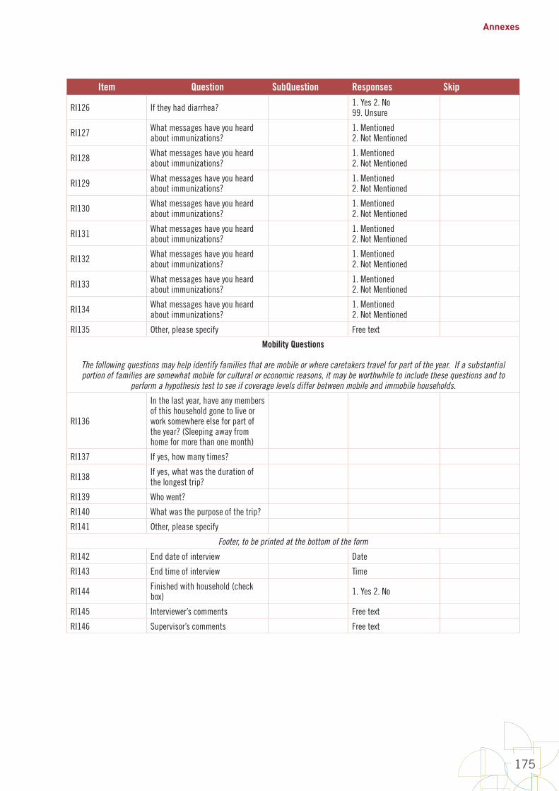
Annexes
175
Item Question SubQuestion Responses Skip
RI126 If they had diarrhea? 1. Yes 2. No99. Unsure
RI127 What messages have you heard about immunizations?
1. Mentioned 2. Not Mentioned
RI128 What messages have you heard about immunizations?
1. Mentioned 2. Not Mentioned
RI129 What messages have you heard about immunizations?
1. Mentioned 2. Not Mentioned
RI130 What messages have you heard about immunizations?
1. Mentioned 2. Not Mentioned
RI131 What messages have you heard about immunizations?
1. Mentioned 2. Not Mentioned
RI132 What messages have you heard about immunizations?
1. Mentioned 2. Not Mentioned
RI133 What messages have you heard about immunizations?
1. Mentioned 2. Not Mentioned
RI134 What messages have you heard about immunizations?
1. Mentioned 2. Not Mentioned
RI135 Other, please specify Free text
Mobility Questions
The following questions may help identify families that are mobile or where caretakers travel for part of the year. If a substantial portion of families are somewhat mobile for cultural or economic reasons, it may be worthwhile to include these questions and to
perform a hypothesis test to see if coverage levels differ between mobile and immobile households.
RI136
In the last year, have any members of this household gone to live or work somewhere else for part of the year? (Sleeping away from home for more than one month)
RI137 If yes, how many times?
RI138 If yes, what was the duration of the longest trip?
RI139 Who went?
RI140 What was the purpose of the trip?
RI141 Other, please specify
Footer, to be printed at the bottom of the form
RI142 End date of interview Date
RI143 End time of interview Time
RI144 Finished with household (check box) 1. Yes 2. No
RI145 Interviewer’s comments Free text
RI146 Supervisor’s comments Free text
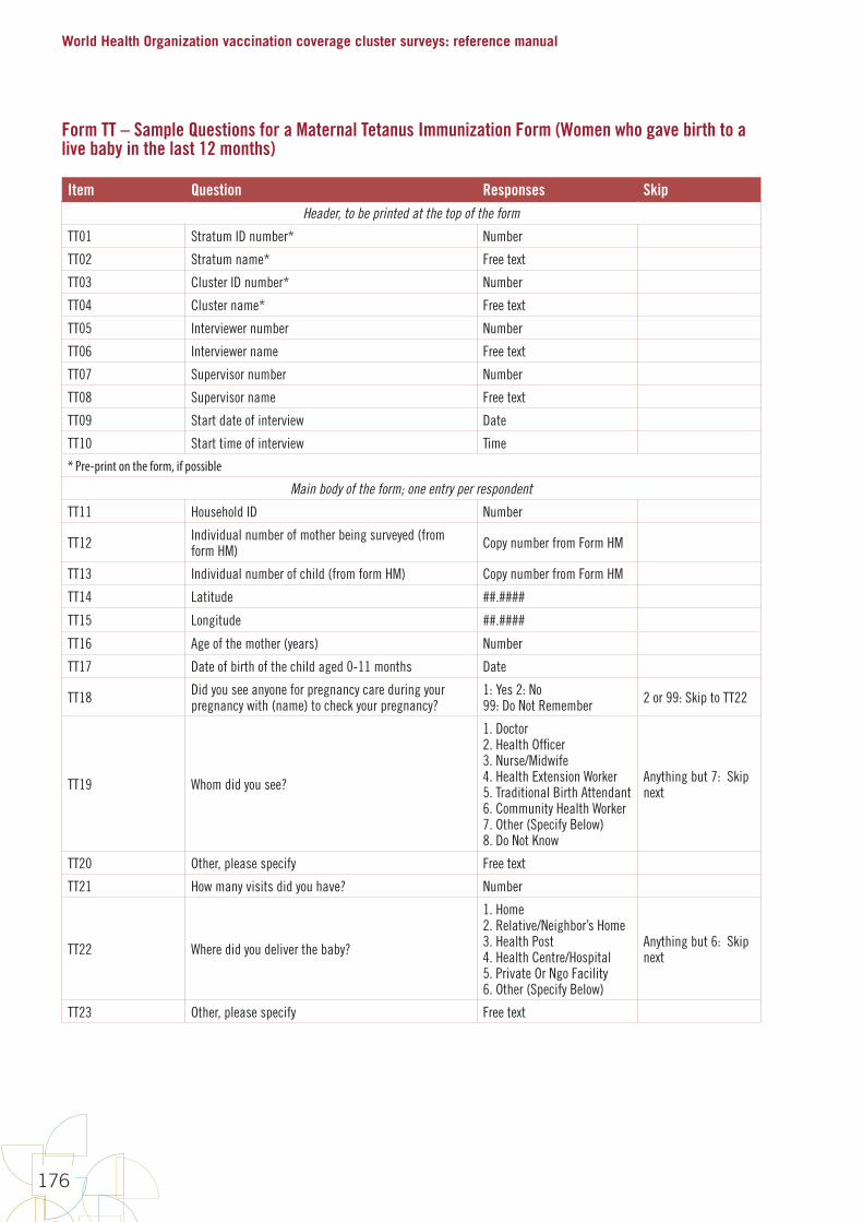
World Health Organization vaccination coverage cluster surveys: reference manual
176
Form TT – Sample Questions for a Maternal Tetanus Immunization Form (Women who gave birth to a live baby in the last 12 months)
Item Question Responses Skip Header, to be printed at the top of the form
TT01 Stratum ID number* Number
TT02 Stratum name* Free text
TT03 Cluster ID number* Number
TT04 Cluster name* Free text
TT05 Interviewer number Number
TT06 Interviewer name Free text
TT07 Supervisor number Number
TT08 Supervisor name Free text
TT09 Start date of interview Date
TT10 Start time of interview Time
* Pre-print on the form, if possible
Main body of the form; one entry per respondent
TT11 Household ID Number
TT12 Individual number of mother being surveyed (from form HM) Copy number from Form HM
TT13 Individual number of child (from form HM) Copy number from Form HM
TT14 Latitude ##.####
TT15 Longitude ##.####
TT16 Age of the mother (years) Number
TT17 Date of birth of the child aged 0-11 months Date
TT18 Did you see anyone for pregnancy care during your pregnancy with (name) to check your pregnancy?
1: Yes 2: No99: Do Not Remember 2 or 99: Skip to TT22
TT19 Whom did you see?
1. Doctor2. Health Officer3. Nurse/Midwife4. Health Extension Worker5. Traditional Birth Attendant6. Community Health Worker7. Other (Specify Below)8. Do Not Know
Anything but 7: Skip next
TT20 Other, please specify Free text
TT21 How many visits did you have? Number
TT22 Where did you deliver the baby?
1. Home 2. Relative/Neighbor’s Home3. Health Post4. Health Centre/Hospital 5. Private Or Ngo Facility 6. Other (Specify Below)
Anything but 6: Skip next
TT23 Other, please specify Free text
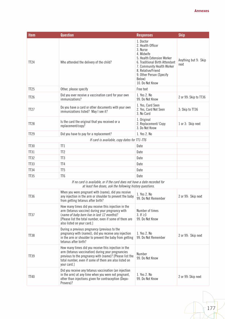
Annexes
177
Item Question Responses Skip
TT24 Who attended the delivery of the child?
1. Doctor 2. Health Officer 3. Nurse 4. Midwife 5. Health Extension Worker 6. Traditional Birth Attendant 7. Community Health Worker 8. Relative/Friend 9. Other Person (Specify Below)10. Do Not Know
Anything but 9: Skip next
TT25 Other, please specify Free text
TT26 Did you ever receive a vaccination card for your own immunizations?
1. Yes 2. No99. Do Not Know 2 or 99: Skip to TT36
TT27 Do you have a card or other documents with your own immunizations listed? May I see it?
1. Yes, Card Seen2. Yes, Card Not Seen3. No Card
3: Skip to TT36
TT28 Is the card the original that you received or a replacement/copy?
1. Original2. Replacement/ Copy3. Do Not Know
1 or 3: Skip next
TT29 Did you have to pay for a replacement? 1. Yes 2. No
If card is available, copy dates for TT1-TT6
TT30 TT1 Date
TT31 TT2 Date
TT32 TT3 Date
TT33 TT4 Date
TT34 TT5 Date
TT35 TT6 Date
If no card is available, or if the card does not have a date recorded for at least five doses, ask the following history questions.
TT36When you were pregnant with (name), did you receive any injection in the arm or shoulder to prevent the baby from getting tetanus after birth?
1. Yes 2. No 99. Do Not Remember 2 or 99: Skip next
TT37
How many times did you receive this injection in the arm (tetanus vaccine) during your pregnancy with (name of baby born live in last 12 months)?[Please list the total number, even if some of them are also listed on your card.]
Number of times3. If ≥399. Do Not Know
TT38
During a previous pregnancy (previous to the pregnancy with (name)), did you receive any injection in the arm or shoulder to prevent the baby from getting tetanus after birth?
1. Yes 2. No 99. Do Not Remember 2 or 99: Skip next
TT39
How many times did you receive this injection in the arm (tetanus vaccination) during your pregnancies previous to the pregnancy with (name)? [Please list the total number, even if some of them are also listed on your card.]
Number99. Do Not Know
TT40
Did you receive any tetanus vaccination (an injection in the arm) at any time when you were not pregnant, other than injections given for contraception (Depo-Provera)?
1. Yes 2. No 99. Do Not Know 2 or 99: Skip next
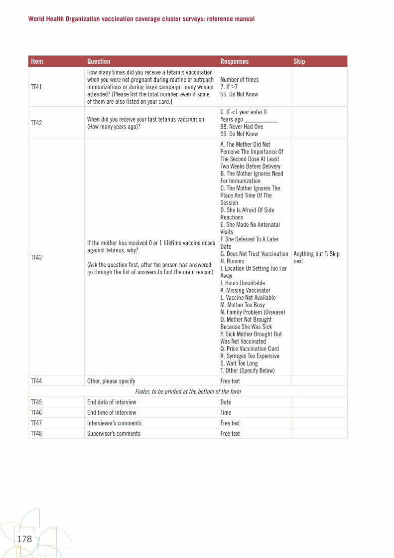
World Health Organization vaccination coverage cluster surveys: reference manual
178
Item Question Responses Skip
TT41
How many times did you receive a tetanus vaccination when you were not pregnant during routine or outreach immunizations or during large campaign many women attended? [Please list the total number, even if some of them are also listed on your card.]
Number of times 7. If ≥7 99. Do Not Know
TT42 When did you receive your last tetanus vaccination (How many years ago)?
0. If <1 year enter 0Years ago __________98. Never Had One99. Do Not Know
TT43
If the mother has received 0 or 1 lifetime vaccine doses against tetanus, why?
(Ask the question first, after the person has answered, go through the list of answers to find the main reason)
A. The Mother Did Not Perceive The Importance Of The Second Dose At Least Two Weeks Before DeliveryB. The Mother Ignores Need For ImmunizationC. The Mother Ignores The Place And Time Of The SessionD. She Is Afraid Of Side ReactionsE. She Made No Antenatal VisitsF. She Deferred To A Later DateG. Does Not Trust VaccinationH. RumorsI. Location Of Setting Too Far AwayJ. Hours UnsuitableK. Missing VaccinatorL. Vaccine Not AvailableM. Mother Too BusyN. Family Problem (Disease) O. Mother Not Brought Because She Was SickP. Sick Mother Brought But Was Not VaccinatedQ. Price Vaccination CardR. Syringes Too ExpensiveS. Wait Too LongT. Other (Specify Below)
Anything but T: Skip next
TT44 Other, please specify Free text
Footer, to be printed at the bottom of the form
TT45 End date of interview Date
TT46 End time of interview Time
TT47 Interviewer’s comments Free text
TT48 Supervisor’s comments Free text
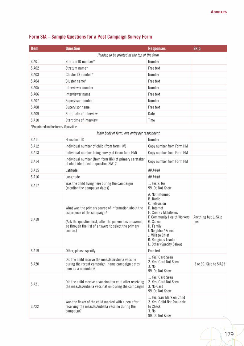
Annexes
179
Form SIA – Sample Questions for a Post Campaign Survey Form
Item Question Responses SkipHeader, to be printed at the top of the form
SIA01 Stratum ID number* Number
SIA02 Stratum name* Free text
SIA03 Cluster ID number* Number
SIA04 Cluster name* Free text
SIA05 Interviewer number Number
SIA06 Interviewer name Free text
SIA07 Supervisor number Number
SIA08 Supervisor name Free text
SIA09 Start date of interview Date
SIA10 Start time of interview Time
*Preprinted on the forms, if possible
Main body of form; one entry per respondent
SIA11 Household ID Number
SIA12 Individual number of child (from form HM) Copy number from Form HM
SIA13 Individual number being surveyed (from form HM) Copy number from Form HM
SIA14 Individual number (from form HM) of primary caretaker of child identified in question SIA12 Copy number from Form HM
SIA15 Latitude ##.####
SIA16 Longitude ##.####
SIA17 Was the child living here during the campaign? (mention the campaign dates)
1. Yes 2. No99. Do Not Know
SIA18
What was the primary source of information about the occurrence of the campaign?
(Ask the question first, after the person has answered, go through the list of answers to select the primary source.)
A. Not InformedB. RadioC. TelevisionD. InternetE. Criers / MobilisersF. Community Health WorkersG. SchoolH. FamilyI. Neighbor/ FriendJ. Village ChiefK. Religious LeaderL. Other (Specify Below)
Anything but L: Skip next
SIA19 Other, please specify Free text
SIA20Did the child receive the measles/rubella vaccine during the recent campaign (name campaign dates here as a reminder)?
1. Yes, Card Seen2. Yes, Card Not Seen3. No 99. Do Not Know
3 or 99: Skip to SIA25
SIA21 Did the child receive a vaccination card after receiving the measles/rubella vaccination during the campaign?
1. Yes, Card Seen2. Yes, Card Not Seen3. No Card99. Do Not Know
SIA22Was the finger of the child marked with a pen after receiving the measles/rubella vaccine during the campaign?
1. Yes, Saw Mark on Child2. Yes, Child Not Available to Check3. No99. Do Not Know
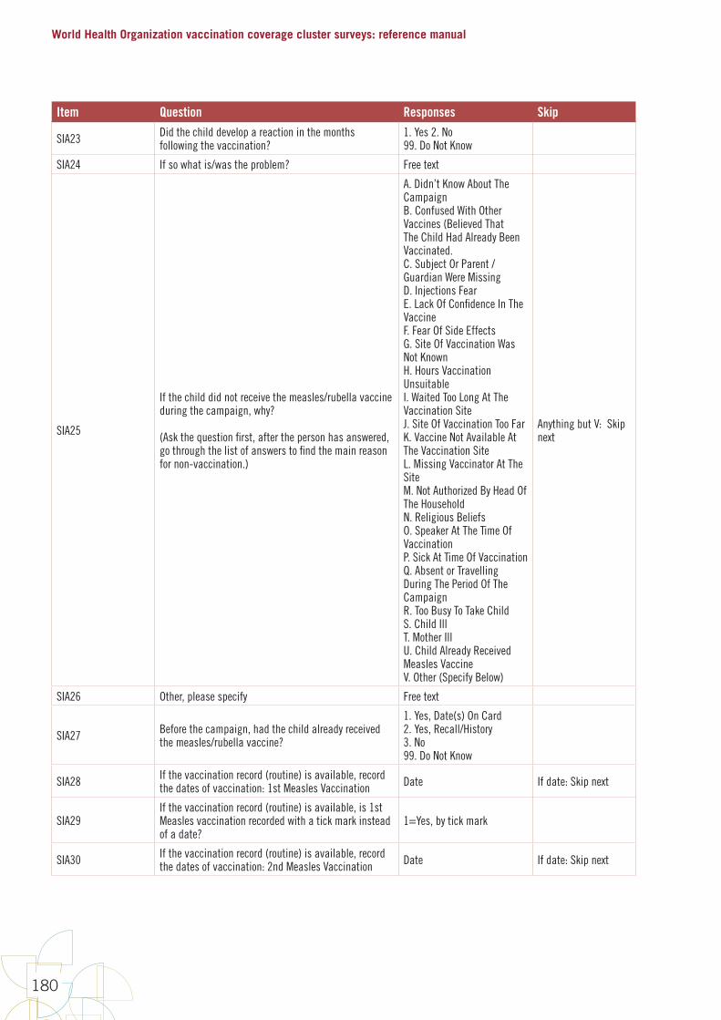
World Health Organization vaccination coverage cluster surveys: reference manual
180
Item Question Responses Skip
SIA23 Did the child develop a reaction in the months following the vaccination?
1. Yes 2. No99. Do Not Know
SIA24 If so what is/was the problem? Free text
SIA25
If the child did not receive the measles/rubella vaccine during the campaign, why?
(Ask the question first, after the person has answered, go through the list of answers to find the main reason for non-vaccination.)
A. Didn’t Know About The CampaignB. Confused With Other Vaccines (Believed That The Child Had Already Been Vaccinated.C. Subject Or Parent / Guardian Were MissingD. Injections FearE. Lack Of Confidence In The VaccineF. Fear Of Side EffectsG. Site Of Vaccination Was Not KnownH. Hours Vaccination UnsuitableI. Waited Too Long At The Vaccination SiteJ. Site Of Vaccination Too FarK. Vaccine Not Available At The Vaccination SiteL. Missing Vaccinator At The SiteM. Not Authorized By Head Of The HouseholdN. Religious BeliefsO. Speaker At The Time Of VaccinationP. Sick At Time Of VaccinationQ. Absent or Travelling During The Period Of The CampaignR. Too Busy To Take ChildS. Child IllT. Mother IllU. Child Already Received Measles VaccineV. Other (Specify Below)
Anything but V: Skip next
SIA26 Other, please specify Free text
SIA27 Before the campaign, had the child already received the measles/rubella vaccine?
1. Yes, Date(s) On Card2. Yes, Recall/History3. No99. Do Not Know
SIA28 If the vaccination record (routine) is available, record the dates of vaccination: 1st Measles Vaccination Date If date: Skip next
SIA29If the vaccination record (routine) is available, is 1st Measles vaccination recorded with a tick mark instead of a date?
1=Yes, by tick mark
SIA30 If the vaccination record (routine) is available, record the dates of vaccination: 2nd Measles Vaccination Date If date: Skip next
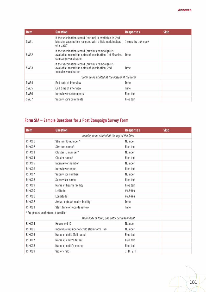
Annexes
181
Item Question Responses Skip
SIA31If the vaccination record (routine) is available, is 2nd Measles vaccination recorded with a tick mark instead of a date?
1=Yes, by tick mark
SIA32If the vaccination record (previous campaign) is available, record the dates of vaccination: 1st Measles campaign vaccination
Date
SIA33If the vaccination record (previous campaign) is available, record the dates of vaccination: 2nd measles vaccination
Date
Footer, to be printed at the bottom of the form
SIA34 End date of interview Date
SIA35 End time of interview Time
SIA36 Interviewer’s comments Free text
SIA37 Supervisor’s comments Free text
Form SIA – Sample Questions for a Post Campaign Survey Form
Item Question Responses SkipHeader, to be printed at the top of the form
RIHC01 Stratum ID number* Number
RIHC02 Stratum name* Free text
RIHC03 Cluster ID number* Number
RIHC04 Cluster name* Free text
RIHC05 Interviewer number Number
RIHC06 Interviewer name Free text
RIHC07 Supervisor number Number
RIHC08 Supervisor name Free text
RIHC09 Name of health facility Free text
RIHC10 Latitude ##.####
RIHC11 Longitude ##.####
RIHC12 Arrival date at health facility Date
RIHC13 Start time of records review Time
* Pre-printed on the form, if possible
Main body of form; one entry per respondent
RIHC14 Household ID Number
RIHC15 Individual number of child (from form HM) Number
RIHC16 Name of child (full name) Free text
RIHC17 Name of child's father Free text
RIHC18 Name of child's mother Free text
RIHC19 Sex of child 1. M 2. F
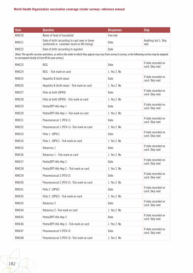
World Health Organization vaccination coverage cluster surveys: reference manual
182
Item Question Responses SkipRIHC20 Name of head of household Free text
RIHC21 Date of birth (according to card seen in home (preferred) or caretaker recall on HH listing) Date Anything but L: Skip
next
RIHC22 Date of birth (according to register) Date
(Note: The specific vaccines and doses, as well as the order in which they appear may vary from survey to survey, so the following section may be adapted to correspond closely to Form RI for your survey.)
RIHC23 BCG Date If date recorded on card: Skip next
RIHC24 BCG - Tick mark on card 1. Yes 2. No
RIHC25 Hepatitis B (birth dose) Date If date recorded on card: Skip next
RIHC26 Hepatitis B (birth dose) - Tick mark on card 1. Yes 2. No
RIHC27 Polio at birth (OPV0) Date If date recorded on card: Skip next
RIHC28 Polio at birth (OPV0) - Tick mark on card 1. Yes 2. No
RIHC29 Penta/DPT-Hib-Hep 1 Date If date recorded on card: Skip next
RIHC30 Penta/DPT-Hib-Hep 1- Tick mark on card 1. Yes 2. No
RIHC31 Pneumococcal 1 (PCV-1) Date If date recorded on card: Skip next
RIHC32 Pneumococcal 1 (PCV-1)- Tick mark on card 1. Yes 2. No
RIHC33 Polio 1 (OPV1) Date If date recorded on card: Skip next
RIHC34 Polio 1 (OPV1) - Tick mark on card 1. Yes 2. No
RIHC35 Rotavirus 1 Date If date recorded on card: Skip next
RIHC36 Rotavirus 1 - Tick mark on card 1. Yes 2. No
RIHC37 Penta/DPT-Hib-Hep 2 Date If date recorded on card: Skip next
RIHC38 Penta/DPT-Hib-Hep 2 - Tick mark on card 1. Yes 2. No
RIHC39 Pneumococcal 2 (PCV-2) Date If date recorded on card: Skip next
RIHC40 Pneumococcal 2 (PCV-2)- Tick mark on card 1. Yes 2. No
RIHC41 Polio 2 (OPV2) Date If date recorded on card: Skip next
RIHC42 Polio 2 (OPV2) - Tick mark on card 1. Yes 2. No
RIHC43 Rotavirus 2 Date If date recorded on card: Skip next
RIHC44 Rotavirus 2- Tick mark on card 1. Yes 2. No
RIHC45 Penta/DPT-Hib-Hep 3 Date If date recorded on card: Skip next
RIHC46 Penta/DPT-Hib-Hep 3 - Tick mark on card 1. Yes 2. No
RIHC47 Pneumococcal 3 (PCV-3) Date If date recorded on card: Skip next
RIHC48 Pneumococcal 3 (PCV-3)- Tick mark on card 1. Yes 2. No
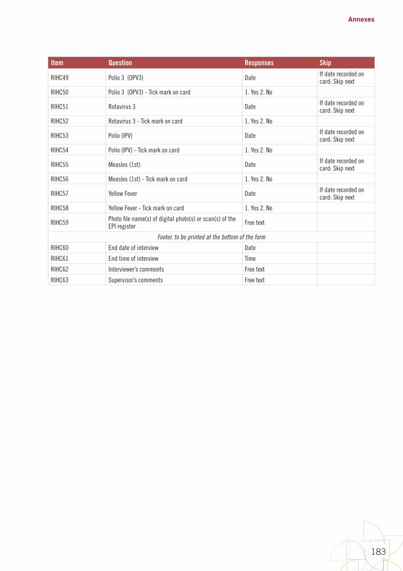
Annexes
183
Item Question Responses Skip
RIHC49 Polio 3 (OPV3) Date If date recorded on card: Skip next
RIHC50 Polio 3 (OPV3) - Tick mark on card 1. Yes 2. No
RIHC51 Rotavirus 3 Date If date recorded on card: Skip next
RIHC52 Rotavirus 3 - Tick mark on card 1. Yes 2. No
RIHC53 Polio (IPV) Date If date recorded on card: Skip next
RIHC54 Polio (IPV) - Tick mark on card 1. Yes 2. No
RIHC55 Measles (1st) Date If date recorded on card: Skip next
RIHC56 Measles (1st) - Tick mark on card 1. Yes 2. No
RIHC57 Yellow Fever Date If date recorded on card: Skip next
RIHC58 Yellow Fever - Tick mark on card 1. Yes 2. No
RIHC59 Photo file name(s) of digital photo(s) or scan(s) of the EPI register Free text
Footer, to be printed at the bottom of the form
RIHC60 End date of interview Date
RIHC61 End time of interview Time
RIHC62 Interviewer’s comments Free text
RIHC63 Supervisor’s comments Free text
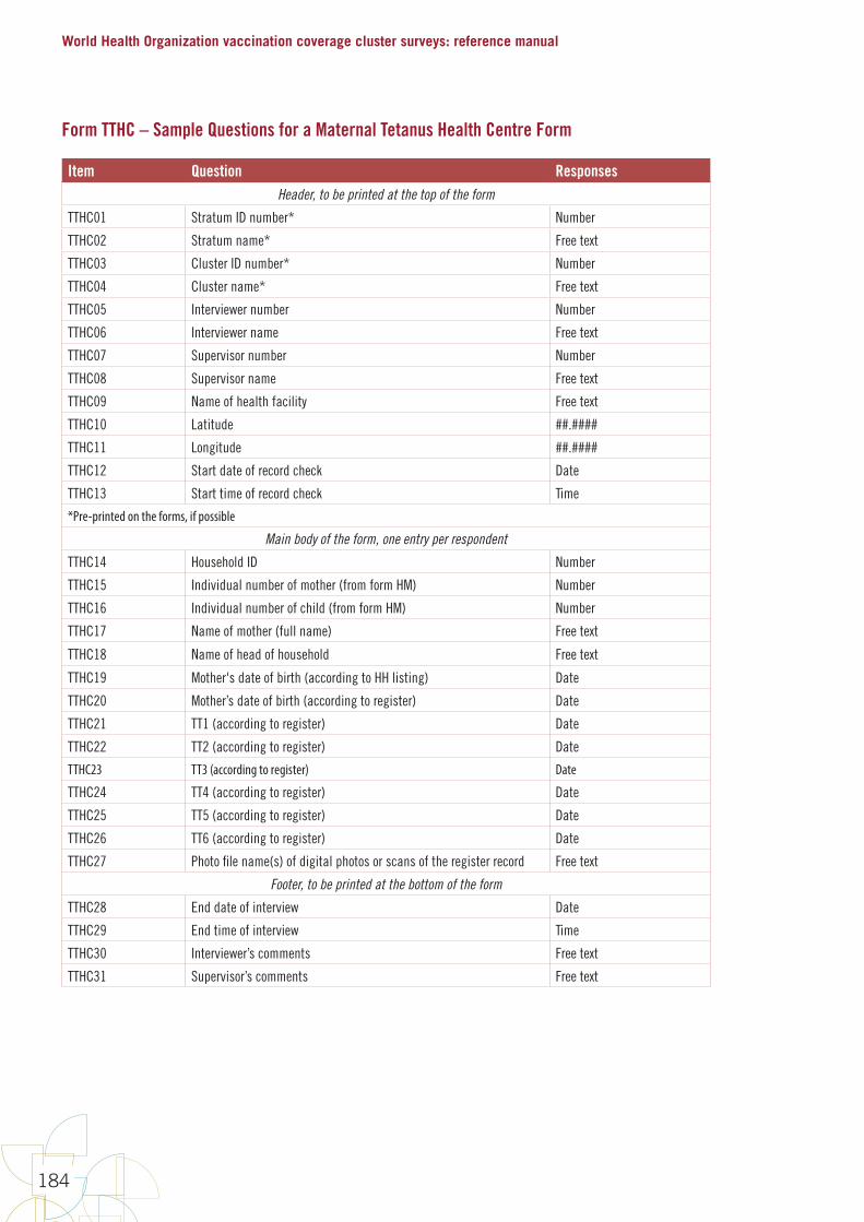
World Health Organization vaccination coverage cluster surveys: reference manual
184
Form TTHC – Sample Questions for a Maternal Tetanus Health Centre Form
Item Question ResponsesHeader, to be printed at the top of the form
TTHC01 Stratum ID number* Number
TTHC02 Stratum name* Free text
TTHC03 Cluster ID number* Number
TTHC04 Cluster name* Free text
TTHC05 Interviewer number Number
TTHC06 Interviewer name Free text
TTHC07 Supervisor number Number
TTHC08 Supervisor name Free text
TTHC09 Name of health facility Free text
TTHC10 Latitude ##.####
TTHC11 Longitude ##.####
TTHC12 Start date of record check Date
TTHC13 Start time of record check Time
*Pre-printed on the forms, if possible
Main body of the form, one entry per respondent
TTHC14 Household ID Number
TTHC15 Individual number of mother (from form HM) Number
TTHC16 Individual number of child (from form HM) Number
TTHC17 Name of mother (full name) Free text
TTHC18 Name of head of household Free text
TTHC19 Mother's date of birth (according to HH listing) Date
TTHC20 Mother’s date of birth (according to register) Date
TTHC21 TT1 (according to register) Date
TTHC22 TT2 (according to register) Date
TTHC23 TT3 (according to register) Date
TTHC24 TT4 (according to register) Date
TTHC25 TT5 (according to register) Date
TTHC26 TT6 (according to register) Date
TTHC27 Photo file name(s) of digital photos or scans of the register record Free text
Footer, to be printed at the bottom of the form
TTHC28 End date of interview Date
TTHC29 End time of interview Time
TTHC30 Interviewer’s comments Free text
TTHC31 Supervisor’s comments Free text
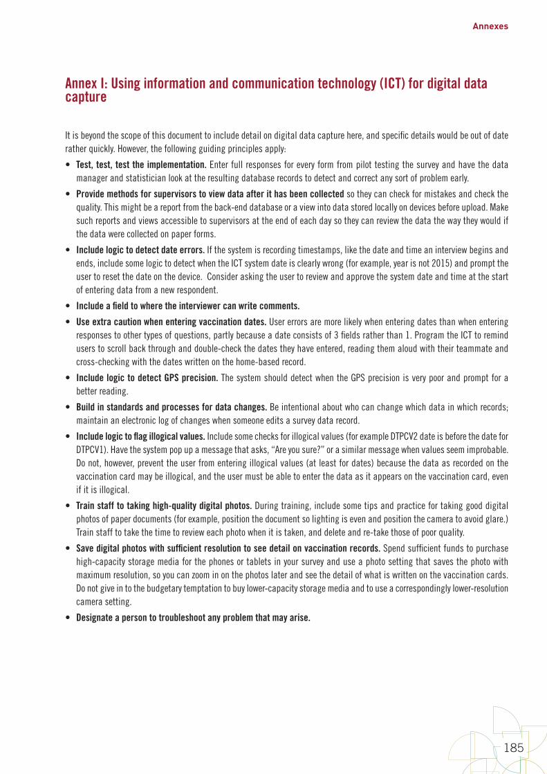
Annexes
185
Annex I: Using information and communication technology (ICT) for digital data capture
It is beyond the scope of this document to include detail on digital data capture here, and specific details would be out of date rather quickly. However, the following guiding principles apply:
• Test, test, test the implementation. Enter full responses for every form from pilot testing the survey and have the data manager and statistician look at the resulting database records to detect and correct any sort of problem early.
• Provide methods for supervisors to view data after it has been collected so they can check for mistakes and check the quality. This might be a report from the back-end database or a view into data stored locally on devices before upload. Make such reports and views accessible to supervisors at the end of each day so they can review the data the way they would if the data were collected on paper forms.
• Include logic to detect date errors. If the system is recording timestamps, like the date and time an interview begins and ends, include some logic to detect when the ICT system date is clearly wrong (for example, year is not 2015) and prompt the user to reset the date on the device. Consider asking the user to review and approve the system date and time at the start of entering data from a new respondent.
• Include a field to where the interviewer can write comments.
• Use extra caution when entering vaccination dates. User errors are more likely when entering dates than when entering responses to other types of questions, partly because a date consists of 3 fields rather than 1. Program the ICT to remind users to scroll back through and double-check the dates they have entered, reading them aloud with their teammate and cross-checking with the dates written on the home-based record.
• Include logic to detect GPS precision. The system should detect when the GPS precision is very poor and prompt for a better reading.
• Build in standards and processes for data changes. Be intentional about who can change which data in which records; maintain an electronic log of changes when someone edits a survey data record.
• Include logic to flag illogical values. Include some checks for illogical values (for example DTPCV2 date is before the date for DTPCV1). Have the system pop up a message that asks, “Are you sure?” or a similar message when values seem improbable. Do not, however, prevent the user from entering illogical values (at least for dates) because the data as recorded on the vaccination card may be illogical, and the user must be able to enter the data as it appears on the vaccination card, even if it is illogical.
• Train staff to taking high-quality digital photos. During training, include some tips and practice for taking good digital photos of paper documents (for example, position the document so lighting is even and position the camera to avoid glare.) Train staff to take the time to review each photo when it is taken, and delete and re-take those of poor quality.
• Save digital photos with sufficient resolution to see detail on vaccination records. Spend sufficient funds to purchase high-capacity storage media for the phones or tablets in your survey and use a photo setting that saves the photo with maximum resolution, so you can zoom in on the photos later and see the detail of what is written on the vaccination cards. Do not give in to the budgetary temptation to buy lower-capacity storage media and to use a correspondingly lower-resolution camera setting.
• Designate a person to troubleshoot any problem that may arise.
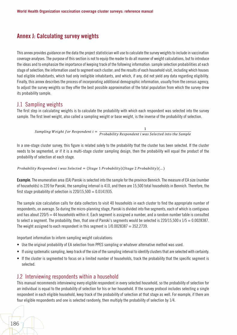
World Health Organization vaccination coverage cluster surveys: reference manual
186
Annex J: Calculating survey weights
This annex provides guidance on the data the project statistician will use to calculate the survey weights to include in vaccination coverage analyses. The purpose of this section is not to equip the reader to do all manner of weight calculations, but to introduce the ideas and to emphasize the importance of keeping track of the following information: sample selection probabilities at each stage of selection; the information used to segment each cluster; and the results of each household visit, including which houses had eligible inhabitants, which had only ineligible inhabitants, and which, if any, did not yield any data regarding eligibility. Finally, this annex describes the process of incorporating additional demographic information, usually from the census agency, to adjust the survey weights so they offer the best possible approximation of the total population from which the survey drew its probability sample.
J.1 Sampling weightsThe first step in calculating weights is to calculate the probability with which each respondent was selected into the survey sample. The first level weight, also called a sampling weight or base weight, is the inverse of the probability of selection.
J-1
Annex J: Calculating survey weights Thisannexprovidesguidanceonthedatatheprojectstatisticianwillusetocalculatethesurveyweightstoincludeinvaccinationcoverageanalyses.Thepurposeofthissectionisnottoequipthereadertodoallmannerofweightcalculations,buttointroducetheideasandtoemphasizetheimportanceofkeepingtrackofthefollowinginformation:sampleselectionprobabilitiesateachstageofselection;theinformationusedtosegmenteachcluster;andtheresultsofeachhouseholdvisit,includingwhichhouseshadeligibleinhabitants,whichhadonlyineligibleinhabitants,andwhich,ifany,didnotyieldanydataregardingeligibility.Finally,thisannexdescribestheprocessofincorporatingadditionaldemographicinformation,usuallyfromthecensusagency,toadjustthesurveyweightssotheyofferthebestpossibleapproximationofthetotalpopulationfromwhichthesurveydrewitsprobabilitysample.
J.1 Sampling weights Thefirststepincalculatingweightsistocalculatetheprobabilitywithwhicheachrespondentwasselectedintothesurveysample.Thefirstlevelweight,alsocalledasamplingweightorbaseweight,istheinverseoftheprobabilityofselection.
"DMeBg)hfAghℎCjkIlAmek)3A)Cg = 1?IknDngBgColAmek)3A)CgpDm"ABAqCA3g)CkCℎA"DMeBA
Inaone-stageclustersurvey,thisfigureisrelatedsolelytotheprobabilitythattheclusterhasbeenselected.Iftheclusterneedstobesegmented,orifitisamulti-stageclustersamplingdesign,thentheprobabilitywillequaltheproductoftheprobabilityofselectionateachstage.
?IknDngBgColAmek)3A)CgpDm"ABAqCA3 = "CDhA1?IknDngBgCo "CDhA2?IknDngBgCo (… )
Example.Theenumerationarea(EA)PanskiisselectedintothesamplefortheprovinceBennich.ThemeasureofEAsize(numberofhouseholds)is220forPanski,thesamplingintervalis410,andthereare15,500totalhouseholdsinBennich.Therefore,thefirststageprobabilityofselectionis220/15,500=0.0141935.
Thesamplesizecalculationcallsfordatacollectorstovisit40householdsineachclustertofindtheappropriatenumberofrespondents,onaverage.Soduringthemicro-planningstage,Bennichisdividedintofivesegments,eachofwhichiscontiguousandhasabout220/4=44householdswithinit.Eachsegmentisassignedanumber,andarandomnumbertableisconsultedtoselectasegment.Theprobability,then,thatPanskiwouldbeselectedis220/15,500x1/5=0.0028387.Theweightassignedtoeachrespondentinthissegmentis1/0.0028387=352.2739.
Importantinformationtoinformsamplingweightcalculations:
• UsetheoriginalprobabilityofEAselectionfromPPESsamplingorwhateveralternativemethodwasused.
• Ifusingsystematicsampling,keeptrackofthesizeofthesamplingintervaltoidentifyclustersthatareselectedwithcertainty.
In a one-stage cluster survey, this figure is related solely to the probability that the cluster has been selected. If the cluster needs to be segmented, or if it is a multi-stage cluster sampling design, then the probability will equal the product of the probability of selection at each stage.
J-1
Annex J: Calculating survey weights Thisannexprovidesguidanceonthedatatheprojectstatisticianwillusetocalculatethesurveyweightstoincludeinvaccinationcoverageanalyses.Thepurposeofthissectionisnottoequipthereadertodoallmannerofweightcalculations,buttointroducetheideasandtoemphasizetheimportanceofkeepingtrackofthefollowinginformation:sampleselectionprobabilitiesateachstageofselection;theinformationusedtosegmenteachcluster;andtheresultsofeachhouseholdvisit,includingwhichhouseshadeligibleinhabitants,whichhadonlyineligibleinhabitants,andwhich,ifany,didnotyieldanydataregardingeligibility.Finally,thisannexdescribestheprocessofincorporatingadditionaldemographicinformation,usuallyfromthecensusagency,toadjustthesurveyweightssotheyofferthebestpossibleapproximationofthetotalpopulationfromwhichthesurveydrewitsprobabilitysample.
J.1 Sampling weights Thefirststepincalculatingweightsistocalculatetheprobabilitywithwhicheachrespondentwasselectedintothesurveysample.Thefirstlevelweight,alsocalledasamplingweightorbaseweight,istheinverseoftheprobabilityofselection.
"DMeBg)hfAghℎCjkIlAmek)3A)Cg = 1?IknDngBgColAmek)3A)CgpDm"ABAqCA3g)CkCℎA"DMeBA
Inaone-stageclustersurvey,thisfigureisrelatedsolelytotheprobabilitythattheclusterhasbeenselected.Iftheclusterneedstobesegmented,orifitisamulti-stageclustersamplingdesign,thentheprobabilitywillequaltheproductoftheprobabilityofselectionateachstage.
?IknDngBgColAmek)3A)CgpDm"ABAqCA3 = "CDhA1?IknDngBgCo "CDhA2?IknDngBgCo (… )
Example.Theenumerationarea(EA)PanskiisselectedintothesamplefortheprovinceBennich.ThemeasureofEAsize(numberofhouseholds)is220forPanski,thesamplingintervalis410,andthereare15,500totalhouseholdsinBennich.Therefore,thefirststageprobabilityofselectionis220/15,500=0.0141935.
Thesamplesizecalculationcallsfordatacollectorstovisit40householdsineachclustertofindtheappropriatenumberofrespondents,onaverage.Soduringthemicro-planningstage,Bennichisdividedintofivesegments,eachofwhichiscontiguousandhasabout220/4=44householdswithinit.Eachsegmentisassignedanumber,andarandomnumbertableisconsultedtoselectasegment.Theprobability,then,thatPanskiwouldbeselectedis220/15,500x1/5=0.0028387.Theweightassignedtoeachrespondentinthissegmentis1/0.0028387=352.2739.
Importantinformationtoinformsamplingweightcalculations:
• UsetheoriginalprobabilityofEAselectionfromPPESsamplingorwhateveralternativemethodwasused.
• Ifusingsystematicsampling,keeptrackofthesizeofthesamplingintervaltoidentifyclustersthatareselectedwithcertainty.
Example. The enumeration area (EA) Panski is selected into the sample for the province Bennich. The measure of EA size (number of households) is 220 for Panski, the sampling interval is 410, and there are 15,500 total households in Bennich. Therefore, the first stage probability of selection is 220/15,500 = 0.0141935.
The sample size calculation calls for data collectors to visit 40 households in each cluster to find the appropriate number of respondents, on average. So during the micro-planning stage, Panski is divided into five segments, each of which is contiguous and has about 220/5 = 44 households within it. Each segment is assigned a number, and a random number table is consulted to select a segment. The probability, then, that one of Panski's segments would be selected is 220/15,500 x 1/5 = 0.0028387. The weight assigned to each respondent in this segment is 1/0.0028387 = 352.2739.
Important information to inform sampling weight calculations:
• Use the original probability of EA selection from PPES sampling or whatever alternative method was used.
• If using systematic sampling, keep track of the size of the sampling interval to identify clusters that are selected with certainty.
• If the cluster is segmented to focus on a limited number of households, track the probability that the specific segment is selected.
J.2 Interviewing respondents within a householdThis manual recommends interviewing every eligible respondent in every selected household, so the probability of selection for an individual is equal to the probability of selection for his or her household. If the survey protocol includes selecting a single respondent in each eligible household, keep track of the probability of selection at that stage as well. For example, if there are four eligible respondents and one is selected randomly, then multiply the probability of selection by 1/4.
Annexes
187
J.3 Adjusting for non-responseA full treatment of methods for accounting for missing data is beyond the scope of this manual, but we do provide guidance that empowers survey designers to collect a dataset that will be compatible with modern methods.
The micro-planning for each cluster identifies a fixed set of households to visit. Field data collectors visit every household in the sample. If the respondents are at home and cooperative in every home, there will be no missing data, and no extra uncertainty in the survey results due to missing data. In most circumstances, though, there will be missing data of some kind:
• There may be entire clusters missing due to natural disaster, war, or other safety concerns.
• Entire households may be missing because no one was at home, despite repeated visits. It will be helpful to collect some information from neighbours when respondents are not at home.
» Establish a protocol for asking neighbours whether there are eligible respondents living in the homes where no one is at home.
» Record this information in a manner that can be coded in the dataset.
⁰ This will help with adjusting for non-response.
⁰ It will also be helpful information during survey data collection, as the team can be sure to revisit those households that are most likely to have eligible respondents.
• Data may be missing from individual respondents, because the caretaker was not available or refused to participate.
• The data for single questions may be missing because respondents don’t know or refuse to answer, or data collectors mistakenly skip a question they should have asked.
Missing data can affect survey weights in several ways. All eligible respondents in the selected households should have a survey weight. If there are households for which you do not know whether occupants were eligible, an adjustment may be made to transfer the weight eligible respondents might have had, if you knew about them, to households for which you do know about eligibility. See Valliant, et al. 2013 for a discussion of this adjustment. The statistician can use the information from homes with respondents to estimate the number of eligible respondents that would have likely been in the homes with no information about eligibility, and then allocate the weight from those missing respondents across the households that responded to the survey.
When there are eligible respondents whose responses are missing, the survey analysis plan should specify the method that will be used to account for extra uncertainty due to not knowing what those responses might have been. Some missing data techniques will involve adjusting survey weights, and some will not. If the survey dataset includes information on the outcome of every visit to every household in the sample, the statistician will be able to construct an analysis plan and conduct analyses that adjust for non-response.
Important information to inform adjustment for non-response:
• description in the analysis plan of how missing data will be handled: entire clusters, entire households, entire respondents, and individual questions
• indication of whether the field data team obtained any information on the number of eligible respondents for each household
• number of eligible respondents in each household in the survey sample, as identified by an occupant of the household (preferred) or by a neighbour.

World Health Organization vaccination coverage cluster surveys: reference manual
188
J.4 Post-stratification to re-scale survey weightsIt may be possible to use the sum of survey weights in each stratum as a high quality estimate of the relative counts of eligible population. (That is, if the sum of weights in Stratum A is 2X the sum in Stratum B, then we assume that Stratum A holds 2X the number of eligible respondents as Stratum B, and when weights are aggregated across strata, the estimate from A will be given 2X the weight as that from B. Both DHS and MICS use this approach.) To do this, all of the following must be true:
• the survey has access to high quality maps of cluster boundaries;
• does a thorough job of listing all households in each cluster;
• tracks the probability of selection at each stage;
• tracks information necessary to adjust for non-response; and
• each stratum includes about 30 or more clusters.
At the time of this writing, it is uncommon in EPI surveys for all of the conditions described above to be true. When they are not all true, and if the weights are well constructed, the dataset can be used to estimate coverage proportions within individual strata. But the dataset should not be used to aggregate across strata or to estimate totals, like the total number of children vaccinated in a campaign. However, if up-to-date stratum-level total population figures or birth cohort totals are available from the census agency, it is possible to re-scale the weights so they sum up to the desired total.
J-3
Whenthereareeligiblerespondentswhoseresponsesaremissing,thesurveyanalysisplanshouldspecifythemethodthatwillbeusedtoaccountforextrauncertaintyduetonotknowingwhatthoseresponsesmighthavebeen.Somemissingdatatechniqueswillinvolveadjustingsurveyweights,andsomewillnot.Ifthesurveydatasetincludesinformationontheoutcomeofeveryvisittoeveryhouseholdinthesample,thestatisticianwillbeabletoconstructananalysisplanandconductanalysesthatadjustfornon-response.
Importantinformationtoinformadjustmentfornon-response:
• descriptionintheanalysisplanofhowmissingdatawillbehandled:entireclusters,entirehouseholds,entirerespondents,andindividualquestions
• indicationofwhetherthefielddatateamobtainedanyinformationonthenumberofeligiblerespondentsforeachhousehold
• numberofeligiblerespondentsineachhouseholdinthesurveysample,asidentifiedbyanoccupantofthehousehold(preferred)orbyaneighbour.
J.4 Post-stratification to re-scale survey weights Itmaybepossibletousethesumofsurveyweightsineachstratumasahighqualityestimateoftherelativecountsofeligiblepopulation.(Thatis,ifthesumofweightsinStratumAis2XthesuminStratumB,thenweassumethatStratumAholds2XthenumberofeligiblerespondentsasStratumB,andwhenweightsareaggregatedacrossstrata,theestimatefromAwillbegiven2XtheweightasthatfromB.BothDHSandMICSusethisapproach.)Todothis,allofthefollowingmustbetrue:
• thesurveyhasaccesstohighqualitymapsofclusterboundaries;• doesathoroughjoboflistingallhouseholdsineachcluster;• trackstheprobabilityofselectionateachstage;• tracksinformationnecessarytoadjustfornon-response;and• eachstratumincludesabout30ormoreclusters.
Atthetimeofthiswriting,itisuncommoninEPIsurveysforalloftheconditionsdescribedabovetobetrue.Whentheyarenotalltrue,andiftheweightsarewellconstructed,thedatasetcanbeusedtoestimatecoverageproportionswithinindividualstrata.Butthedatasetshouldnotbeusedtoaggregateacrossstrataortoestimatetotals,likethetotalnumberofchildrenvaccinatedinacampaign.However,ifup-to-datestratum-leveltotalpopulationfiguresorbirthcohorttotalsareavailablefromthecensusagency,itispossibletore-scaletheweightssotheysumuptothedesiredtotal.
"qDBA3fAghℎCs = t)mqDBA3fAghℎCs u)kp)!BghgnBA?kevBDCgk)wkCDBjkI"CIDCvM
t)mqDBA3fAghℎCmg)"CIDCvM
Thismethodwouldbealsoapplicableinasituationwheresurveydesignersdecidetooversamplethepopulationinastratumofinterest,relativetotheirportionoftheoverallpopulation,inordertoobtainprecisecoverageestimatesforthatstratum.Beforethedataareaggregatedacrossstrata,theweightsshouldbepost-stratified.
This method would be also applicable in a situation where survey designers decide to oversample the population in a stratum of interest, relative to their portion of the overall population, in order to obtain precise coverage estimates for that stratum. Before the data are aggregated across strata, the weights should be post-stratified.
The census agency may provide information on two or more variables, such as projected total eligible population by sex and also by ethnic group. When these figures are provided as marginal population totals (by sex and ethnic group separately, not every combination of sex and ethnic group) then the process known as raking can be used to post-stratify the weights. See Lohr 2009 or Valliant, et al. 2013 for more details.
Important information to inform post-stratification:
• likely eligible population totals for each geographic stratum (from census agency)
• likely totals for each demographic subgroup of interest within each geographic stratum (from census agency).
J.5 Additional commentsThis manual strongly encourages conducting weighted statistical analysis of vaccination coverage survey data. The statistician should be involved early in the project to make recommendations about how to select the sample, how questions should be ordered and coded on data collection forms, how to adjust for non-response, how to post-stratify or make other adjustments to weights, and how to incorporate weights into the analysis.
At each stage of selection careful work is required to track and record all the elements that go into calculating the weights. During fieldwork careful work is required to record the outcome of every visit to every home. The result of the additional work required to conduct a weighted analysis will be a set of results that are more representative and generalizable than they have been in the past. EPI surveys with careful attention to random selection, appropriate use of survey weights and excellent quality control in data collection will be more comparable to other modern surveys (such as the USAID Demographic and Health Surveys- DHS or UNICEF Multi-Indicator Cluster Surveys-MICS) compared to surveys collected and analysed with earlier EPI cluster survey protocols.
Annexes
189
Annex K: Using software to calculate weighted coverage estimates
Calculating weighted coverage estimates from respondents with completed interviews is straightforward and may be accomplished using any statistical software package. Some techniques for accounting for survey nonresponse may be sophisticated and require special software. Calculating coverage confidence intervals is more complicated than point estimates, and definitely requires software that accounts properly for the complex sample design as well as the survey weights.
The appropriate calculations can all be made using modern survey data analysis software like Stata, R, SAS, SUDAAN, SPSS, Epi Info, and others. Consult the user documentation for your software package to be sure to use commands appropriate for weighted analysis of stratified cluster survey data. Exploratory analyses might be conducted using interactive drop-down menus, but the final calculations to be included in the survey report should use commands that are saved in a program or script or syntax file, so important results are reproducible and auditable.
The WHO makes its Vaccination Coverage Quality Indicators (VCQI) tool freely available. VCQI is a set of Stata programs that estimate coverage in a manner consistent with this manual. For more detail, see the WHO’s immunization coverage webpage: VCQI resources are available on WHO vaccination coverage survey webpage http://www.who.int/immunization/monitoring_surveillance/routine/coverage/en/, under survey methods. The VCQI programs are provided free of charge, but you will need a licensed version of Stata1 version 14 or later to run VCQI, and the license for Stata is not free.
The following are best practices for including information about the software in the survey report:
1. Name the software package used and make the programs available for review.
2. Specify analysis choices and assumptions clearly. Describe how the data were weighted and how non-response is handled in the calculations.
3. Use a method of calculating confidence intervals that yields appropriately asymmetrical intervals when the sample size is modest and the estimated proportion falls close to 0% or 100%. All of the software packages described above can calculate a so-called “logit interval”, which is a fine choice. If possible, we recommend using a Wilson interval with degrees of freedom modified to be appropriate with the complex sample design, as described in Dean & Pagano, 2015. The WHO VCQI tool calculates a Wilson interval with continuity correction, by default, as suggested by Fleiss, 2003.
4. When comparing coverage between subgroups or strata or over time, use a technique like the Rao-Scott chi-squared to account for survey sampling and weights.
5. When classifying coverage, describe the classification rules and results clearly. Portray results graphically as described in Annex M.
6. Be clear about which tables and output are describing the survey sample and do not need confidence intervals. Also be clear about which tables and output are estimating outcomes for the broader population who were eligible for the survey; these results should be accompanied by confidence intervals.
7. Portray results graphically, and include confidence intervals (or bounds, as appropriate) in the graphics.
8. Report clearly which data sources are considered in each result (cards alone, cards and health facility registries, cards and caretaker recall, etc.).
9. Facilitate the planning of future surveys by including an annex in the survey report that lists the calculated design effect and intracluster correlation coefficients from your survey for each important outcome in each stratum and overall.
1 https://www.stata.com/

World Health Organization vaccination coverage cluster surveys: reference manual
190
Annex L: Standard definitions for vaccine coverage indicators
Vaccine coverage indictors are the measures used to assess and track vaccination coverage. Coverage data affect vaccination policies and programmes, so choices about what to measure and how to measure it have a real impact.
Why use standard coverage indicators?
WHO has developed a set of standard coverage indicator definitions for routine immunization surveys, tetanus protection-at-birth surveys and supplemental immunization activity (SIA) surveys. These standard indicators are documented in the documents that accompany WHO’s Vaccination Coverage Quality Indicators (VCQI) tool, a freely available set of Stata programs for analysing vaccination survey data.
Whether you use VCQI or not, calculate and report coverage in a manner consistent with these indicators so the numbers in your report will be comparable with other WHO surveys. Under some circumstances you may wish to define new indicators or to depart from the WHO standards. In every report, be clear about how your coverage indicators are defined and calculated.What information does each standard coverage indicator include?
When you use the WHO indicators or VCQI tool, you can simply reference this manual or the VCQI documentation for coverage indicators. If you choose to calculate different indicators, describe them carefully by including the following information:
• Who is included? Who is excluded?
• How are the denominator and numerator calculated?
• What is the role of weights, if any?
• How are missing data and "do not know" (DNK) responses handled?
• How should the results be interpreted and explained? (For example, do the results apply to the sample only, or to the whole population from which the sample is drawn? Does the indicator include an estimate of sampling uncertainty and, if so, how is it calculated?)
Below is an example of the information you will find for each coverage indicator in the VCQI documentation. This example is for the crude coverage indicator.
RI_COVG_01: Crude coverage
Weighted: Yes
Denominator: Sum of weights for all respondents
Numerator: Sum of weights for respondents who received the vaccine dose per card or recall (or register, if health centres were visited in this survey)
Missing/DNK: All respondents are in the denominator, even if their coverage responses from all sources are missing or “do not know” (DNK). In the numerator, respondents with missing data or DNK responses are considered to have not received the dose.
Interpretation: “X% of the population who were eligible for the survey are estimated to have received <dose>, as documented by <source(s)>.”
Where can I find more information and updates on the standard vaccination coverage indicators?
You can find the full list of updated indicators and definitions in the “VCQI Results Interpretation Quick-Reference Guide.” For guidance on how to calculate derived variables from survey variables, refer to the VCQI “Working List of Vaccination Survey Analyses and Software Specifications.” Both are available at WHO’s Immunization Coverage website: http://www.who.int/immunization/monitoring_surveillance/routine/coverage/en/index2.html.
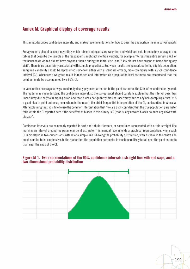
Annexes
191
Annex M: Graphical display of coverage results
This annex describes confidence intervals, and makes recommendations for how to describe and portray them in survey reports
Survey reports should be clear regarding which tables and results are weighted and which are not. Introductory passages and tables that describe the sample or the respondents might not mention weights, for example: “Across the entire survey, 9.6% of the households visited did not have anyone at home during the initial visit, and 7.4% did not have anyone at home during any visit”. There is no uncertainty associated with sample proportions. But when results are generalized to the eligible population, sampling variability should be represented somehow, either with a standard error or, more commonly, with a 95% confidence interval (CI). Whenever a weighted result is reported and interpreted as a population level estimate, we recommend that the point estimate be accompanied by a 95% CI.
In vaccination coverage surveys, readers typically pay most attention to the point estimate; the CI is often omitted or ignored. The reader may misunderstand the confidence interval, so the survey report should carefully explain that the interval describes uncertainty due only to sampling error, and that it does not quantify bias or uncertainty due to any non-sampling errors. It is a good idea to point out once, somewhere in the report, the strict frequentist interpretation of the CI, as described in Annex A. After explaining that, it is fine to use the common interpretation that “we are 95% confident that the true population parameter falls within the CI reported here if the net effect of biases in this survey is 0 (that is, any upward biases balance any downward biases)”.
Confidence intervals are commonly reported in text and tabular formats, or sometimes represented with a thin straight line marking an interval around the parameter point estimate. This manual recommends a graphical representation, where each CI is displayed in two-dimensions instead of a simple line. Showing the probability distribution, with its peak in the centre and much smaller tails, emphasizes to the reader that the population parameter is much more likely to fall near the point estimate than near the ends of the CI.
Figure M-1. Two representations of the 95% confidence interval: a straight line with end caps, and a two-dimensional probability distribution

World Health Organization vaccination coverage cluster surveys: reference manual
192
Three helpful 95% confidence intervals
The manual recommends calculating limits for three helpful 95% CIs. The first interval is illustrated in Figure M-2. Recall that for the traditionally reported 2-sided 95% CI, we represent the probability distribution of the estimated parameter, and we report the point at which 2.5% of the probability falls to the left and 2.5% of the probability falls to the right. (The distributions in Figures M-1 through M-7 are symmetric for purposes of illustration, but for an estimated binomial proportion, the distribution and the 95% CI will be asymmetric when the estimated probability is not 50% and the sample size is not very large. See Figure M-8.)
Figure M-2. The most commonly reported 95% CI is the interval defined by the lowest and highest 2.5% of probability
The second helpful interval is represented in Figure M-3. The lower limit of the interval is the point where 5% of the probability falls to the left and 95% falls to the right. We call the left endpoint the 95% lower confidence bound (LCB). For an estimated proportion, it is also valid to call the interval [LCB, 100%) a 95% CI. When specifying an interval, the square bracket “[”or“]” means that the endpoint is included in the interval, and the parenthesis “(“or“)”is not included in the interval.
Figure M-3. A second useful 95% CI for proportions is defined by the 95% LCB and 1.
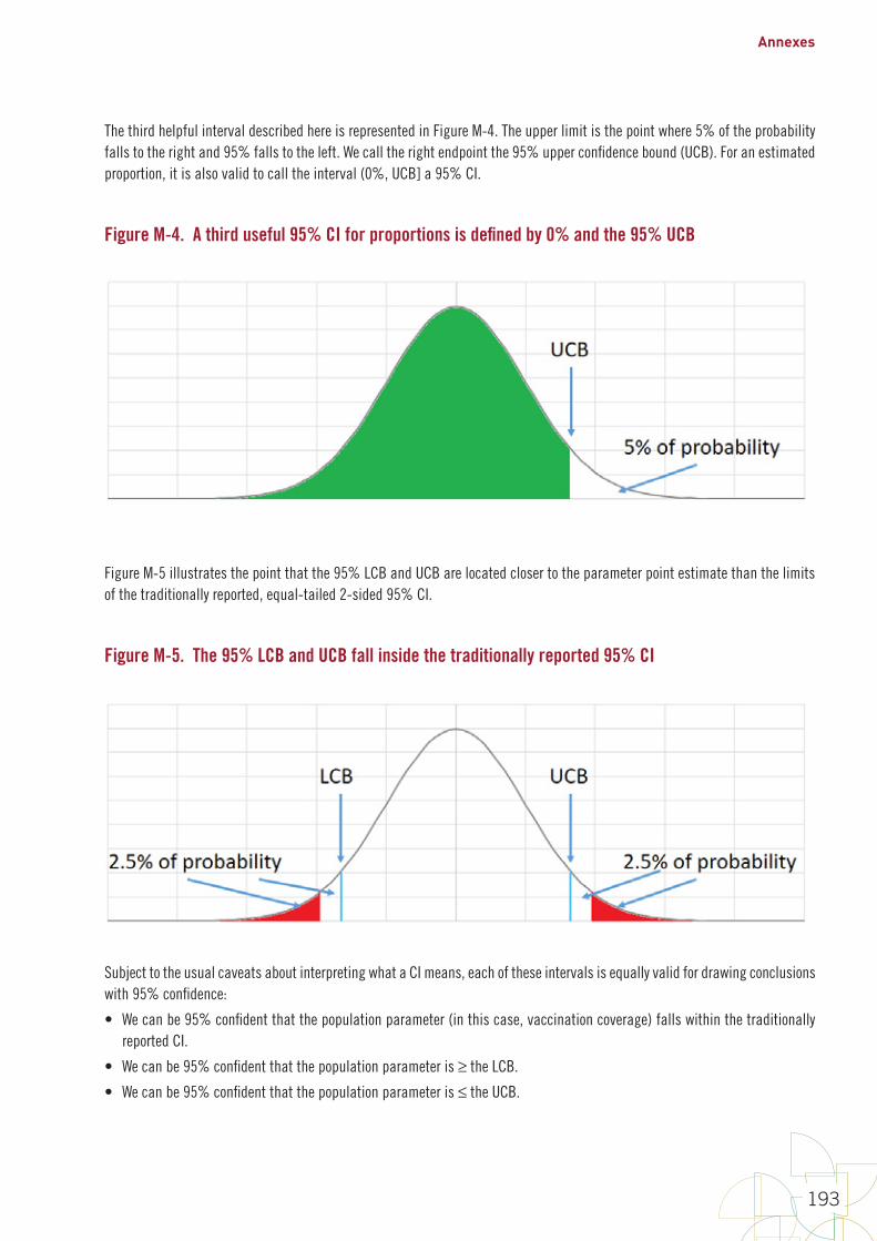
Annexes
193
The third helpful interval described here is represented in Figure M-4. The upper limit is the point where 5% of the probability falls to the right and 95% falls to the left. We call the right endpoint the 95% upper confidence bound (UCB). For an estimated proportion, it is also valid to call the interval (0%, UCB] a 95% CI.
Figure M-4. A third useful 95% CI for proportions is defined by 0% and the 95% UCB
Figure M-5 illustrates the point that the 95% LCB and UCB are located closer to the parameter point estimate than the limits of the traditionally reported, equal-tailed 2-sided 95% CI.
Figure M-5. The 95% LCB and UCB fall inside the traditionally reported 95% CI
Subject to the usual caveats about interpreting what a CI means, each of these intervals is equally valid for drawing conclusions with 95% confidence:
• We can be 95% confident that the population parameter (in this case, vaccination coverage) falls within the traditionally reported CI.
• We can be 95% confident that the population parameter is ≥ the LCB.
• We can be 95% confident that the population parameter is ≤ the UCB.
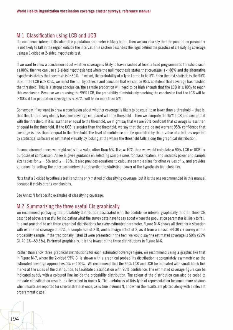
World Health Organization vaccination coverage cluster surveys: reference manual
194
M.1 Classification using LCB and UCBIf a confidence interval tells where the population parameter is likely to fall, then we can also say that the population parameter is not likely to fall in the region outside the interval. This section describes the logic behind the practice of classifying coverage using a 1-sided or 2-sided hypothesis test.
If we want to draw a conclusion about whether coverage is likely to have reached at least a fixed programmatic threshold such as 80%, then we can use a 1-sided hypothesis test where the null hypothesis states that coverage is < 80% and the alternative hypothesis states that coverage is ≥ 80%. If we set, the probability of a Type I error, to be 5%, then the test statistic is the 95% LCB. If the LCB is ≥ 80%, we reject the null hypothesis and conclude that we can be 95% confident that coverage has reached the threshold. This is a strong conclusion: the sample proportion will need to be high enough that the LCB is ≥ 80% to reach this conclusion. Because we are using the 95% LCB, the probability of mistakenly reaching the conclusion that the LCB will be ≥ 80% if the population coverage is < 80%, will be no more than 5%.
Conversely, if we want to draw a conclusion about whether coverage is likely to be equal to or lower than a threshold – that is, that the stratum very clearly has poor coverage compared with the threshold – then we compute the 95% UCB and compare it with the threshold. If it is less than or equal to the threshold, we might say that we are 95% confident that coverage is less than or equal to the threshold. If the UCB is greater than the threshold, we say that the data do not warrant 95% confidence that coverage is less than or equal to the threshold. The level of confidence can be quantified by the p-value of a test, as reported by statistical software or estimated visually by looking at the where the threshold falls along the graphical distribution.
In some circumstances we might set to a value other than 5%. If = 10% then we would calculate a 90% LCB or UCB for purposes of comparison. Annex B gives guidance on selecting sample sizes for classification, and includes power and sample size tables for = 5% and = 10%. It also provides equations to calculate sample sizes for other values of , and provides guidance for setting the other parameters that describe the statistical power of the hypothesis test classifier.
Note that a 1-sided hypothesis test is not the only method of classifying coverage, but it is the one recommended in this manual because it yields strong conclusions.
See Annex N for specific examples of classifying coverage.
M.2 Summarizing the three useful CIs graphicallyWe recommend portraying the probability distribution associated with the confidence interval graphically, and all three CIs described above are useful for indicating what the survey data have to say about where the population parameter is likely to fall. It is not practical to use three graphical distributions for every estimated parameter. Figure M-6 shows all three for a situation with estimated coverage of 50%, a sample size of 210, and a design effect of 2, as if from a classic EPI 30 x 7 survey with a probability sample. If the traditionally listed CI were presented in the text, we would say the estimated coverage is 50% (95% CI: 40.2%–59.8%). Portrayed graphically, it is the lowest of the three distributions in Figure M-6.
Rather than show three graphical distributions for each estimated coverage figure, we recommend using a graphic like that in Figure M-7, where the 2-sided 95% CI is shown with a graphical probability distribution, appropriately asymmetric as the estimated coverage approaches 0% or 100%. We recommend that the 95% LCB and UCB be indicated with small black tick marks at the sides of the distribution, to facilitate classification with 95% confidence. The estimated coverage figure can be indicated subtly with a coloured line inside the probability distribution. The colour of the distribution can also be coded to indicate classification results, as described in Annex N. The usefulness of this type of representation becomes more obvious when results are reported for several strata at once, as is true in Annex N, and when the results are plotted along with a relevant programmatic goal.
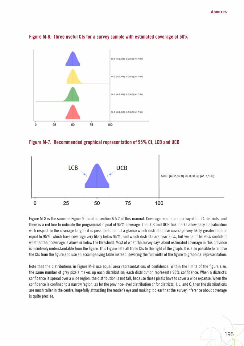
Annexes
195
Figure M-6. Three useful CIs for a survey sample with estimated coverage of 50%
Figure M-7. Recommended graphical representation of 95% CI, LCB and UCB
Figure M-8 is the same as Figure 9 found in section 6.5.2 of this manual. Coverage results are portrayed for 24 districts, and there is a red line to indicate the programmatic goal of 95% coverage. The LCB and UCB tick marks allow easy classification with respect to the coverage target: it is possible to tell at a glance which districts have coverage very likely greater than or equal to 95%, which have coverage very likely below 95%, and which districts are near 95%, but we can’t be 95% confident whether their coverage is above or below the threshold. Most of what the survey says about estimated coverage in this province is intuitively understandable from the figure. This Figure lists all three CIs to the right of the graph. It is also possible to remove the CIs from the figure and use an accompanying table instead, devoting the full width of the figure to graphical representation.
Note that the distributions in Figure M-8 use equal area representations of confidence. Within the limits of the figure size, the same number of grey pixels makes up each distribution; each distribution represents 95% confidence. When a district’s confidence is spread over a wide region, the distribution is not tall, because those pixels have to cover a wide expanse. When the confidence is confined to a narrow region, as for the province-level distribution or for districts H, L, and C, then the distributions are much taller in the centre, hopefully attracting the reader’s eye and making it clear that the survey inference about coverage is quite precise.

World Health Organization vaccination coverage cluster surveys: reference manual
196
The WHO VCQI tool includes a program to make these so-called inchworm plots. See the VCQI documentation to learn more and join the VCQI User’s Group on the TechNet-21 website1 to view tutorials on how to make these plots. It is our hope that this representation will shift attention away from a single-minded focus on coverage point estimates, and intuitively communicate what the survey does and does not tell us about likely coverage levels.
Of course, narrower confidence intervals mean that we have high precision – a good idea of where coverage is likely to fall. While wide CIs mean that our confidence is less focused, even wide CIs give a clear indication of where coverage is likely not to fall, which can often be helpful.
Finally, interpretation of these figures is subject to all the usual caveats that should accompany confidence intervals: if there are important biases in the survey methods or execution, then the true population coverage can fall far below or far above the 95% confidence interval. In order for the CIs to be meaningful, it is important to make every effort to keep biases to an absolute minimum. The survey report should describe efforts to minimize bias in great detail, and should be honest about those biases that may have crept in to the project, so that readers of the report can draw a helpful conclusion about whether the CIs are likely to be meaningful (that is, fall near the true population coverage values). When bias has been minimized, the confidence intervals are useful for purposes of classification, as described in Annex N.
Figure M-8. Graphical coverage survey results for 24 districts and the province that they comprise
1 https://www.technet-21.org/en/network/groups/293-vcqi
Annexes
197
Annex N: Examples of classifying vaccination coverage
In this annex we apply four different classification rules to the same coverage estimation results, and consider the merits of:
• classifying into three categories, high, low and intermediate, rather than using only two categories
• portraying classification results graphically rather than using only tabular output.
N.1 Classifying coverage into categoriesThis manual recommends using upper and lower confidence bounds (usually 95% confidence bounds) to accomplish classification. This is an implementation of a 1-sided hypothesis test. If we apply a single test then we obtain two classification categories, which may be given different labels depending on the context. In this annex we call them pass for high coverage and fail for low coverage. If two hypothesis tests are applied instead, then there could be three outcome categories: high, low, and intermediate.
Figures N-1 through N-4 portray the same data as those in Figure 10 in section 6.4.2 of this manual: estimated measles SIA coverage for 24 fictional districts, based on samples of 15 clusters and 10 respondents per cluster in each district. For each district, the 95% confidence interval is indicated using a coloured probability distribution that has been clipped at the upper and lower limits of the interval. The 95% upper and lower confidence bounds are indicated with small black tick marks.
Three intervals are listed at the right side of each distribution. The first is the classic 2-sided 95% confidence interval. The second is the interval that extends from 0% coverage up to the 95% upper confidence bound. The third is the interval that extends from the 95% lower confidence bound up to coverage of 100%. All three intervals are equally valid for drawing conclusions with 95% confidence. The regions are plotted in increasing order of coverage point estimate, from bottom to top. The red vertical line marks the spot where coverage is 95%, an important programmatic threshold for measles. The district data are aggregated to estimate province coverage (shaded with a light gray bar) very precisely.
The following four classification rules could be applied to the results:
1. A simple rule might use only the point estimate to classify, assigning the label pass to districts where the estimated coverage is greater than or equal to 95% and fail to those with estimated coverage below 95%. See Figure N-1.
2. Another rule might say that districts where the lower 95% confidence bound is greater than or equal to 95% coverage should be designated as pass, and all others should be designated fail. See Figure N-2.
3. Conversely, we could say that any district where the upper 95% confidence bound is less than 95% is designated as fail, and all others are designated pass. See Figure N-3.
4. The final alternative has some important advantages over the previous three: it assigns three labels instead of two. If the lower 95% confidence bound is greater than or equal to 95%, call it pass; if the upper 95% confidence bound is below 95%, call it fail; and otherwise call the results intermediate. See Figure N-4.
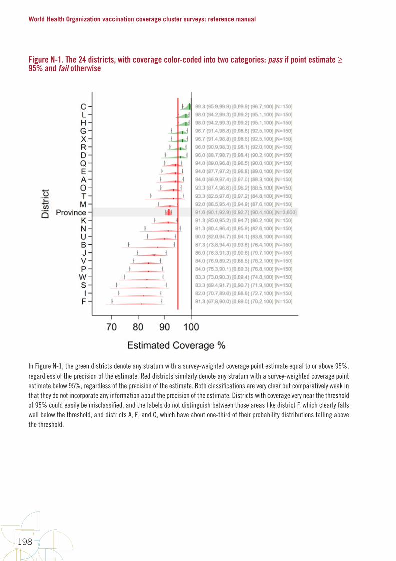
World Health Organization vaccination coverage cluster surveys: reference manual
198
Figure N-1. The 24 districts, with coverage color-coded into two categories: pass if point estimate ≥ 95% and fail otherwise
In Figure N-1, the green districts denote any stratum with a survey-weighted coverage point estimate equal to or above 95%, regardless of the precision of the estimate. Red districts similarly denote any stratum with a survey-weighted coverage point estimate below 95%, regardless of the precision of the estimate. Both classifications are very clear but comparatively weak in that they do not incorporate any information about the precision of the estimate. Districts with coverage very near the threshold of 95% could easily be misclassified, and the labels do not distinguish between those areas like district F, which clearly falls well below the threshold, and districts A, E, and Q, which have about one-third of their probability distributions falling above the threshold.
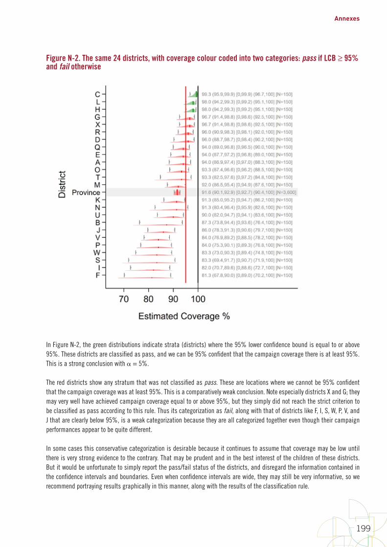
Annexes
199
Figure N-2. The same 24 districts, with coverage colour coded into two categories: pass if LCB ≥ 95% and fail otherwise
In Figure N-2, the green distributions indicate strata (districts) where the 95% lower confidence bound is equal to or above 95%. These districts are classified as pass, and we can be 95% confident that the campaign coverage there is at least 95%. This is a strong conclusion with = 5%.
The red districts show any stratum that was not classified as pass. These are locations where we cannot be 95% confident that the campaign coverage was at least 95%. This is a comparatively weak conclusion. Note especially districts X and G; they may very well have achieved campaign coverage equal to or above 95%, but they simply did not reach the strict criterion to be classified as pass according to this rule. Thus its categorization as fail, along with that of districts like F, I, S, W, P, V, and J that are clearly below 95%, is a weak categorization because they are all categorized together even though their campaign performances appear to be quite different.
In some cases this conservative categorization is desirable because it continues to assume that coverage may be low until there is very strong evidence to the contrary. That may be prudent and in the best interest of the children of these districts. But it would be unfortunate to simply report the pass/fail status of the districts, and disregard the information contained in the confidence intervals and boundaries. Even when confidence intervals are wide, they may still be very informative, so we recommend portraying results graphically in this manner, along with the results of the classification rule.
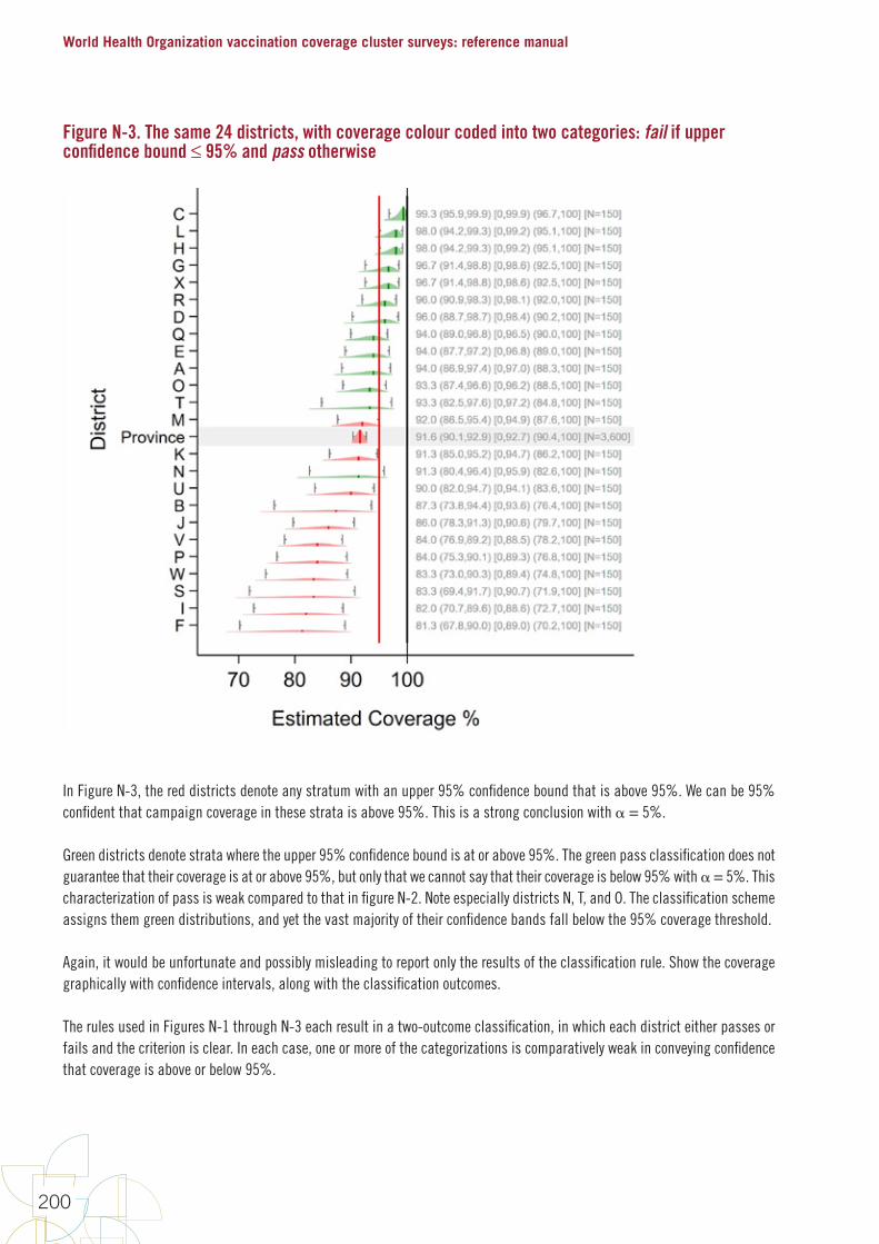
World Health Organization vaccination coverage cluster surveys: reference manual
200
Figure N-3. The same 24 districts, with coverage colour coded into two categories: fail if upper confidence bound ≤ 95% and pass otherwise
In Figure N-3, the red districts denote any stratum with an upper 95% confidence bound that is above 95%. We can be 95% confident that campaign coverage in these strata is above 95%. This is a strong conclusion with = 5%.
Green districts denote strata where the upper 95% confidence bound is at or above 95%. The green pass classification does not guarantee that their coverage is at or above 95%, but only that we cannot say that their coverage is below 95% with = 5%. This characterization of pass is weak compared to that in figure N-2. Note especially districts N, T, and O. The classification scheme assigns them green distributions, and yet the vast majority of their confidence bands fall below the 95% coverage threshold.
Again, it would be unfortunate and possibly misleading to report only the results of the classification rule. Show the coverage graphically with confidence intervals, along with the classification outcomes.
The rules used in Figures N-1 through N-3 each result in a two-outcome classification, in which each district either passes or fails and the criterion is clear. In each case, one or more of the categorizations is comparatively weak in conveying confidence that coverage is above or below 95%.

Annexes
201
A three-outcome scheme that can be informative is portrayed in Figure N-4. The classification rules are as follows:
• If the lower 95% confidence bound is at or above the threshold of interest (for example, 95%), conclude that district coverage is very likely to be at or above 95%.
• If the upper 95% confidence bound is below 95%, conclude that the district coverage is very likely to be below 95%.
• If 95% falls between the lower and upper confidence bounds, conclude that the sample size is too small to say confidently whether the district coverage is above or below 95%. Call this category intermediate.
In Figure N-4, green distributions indicate strata (districts) where the 95% lower confidence bound is at or above 95%. These districts are classified as pass. This is a strong conclusion, and we can be 95% confident that the campaign coverage there is at least 95%.
Red distributions indicate districts where the 95% upper confidence bound is below 95%. These districts are classified as fail. This is a strong conclusion, and we can be 95% confident that the campaign coverage there is below 95%.
Yellow distributions indicate districts with confidence bounds that straddle the 95% threshold, so these data cannot be used to classify them the districts as higher or lower than 95% (pass or fail) at = 5%. We might say that coverage is either too close to 95% or estimated too imprecisely to confidently categorize the district as above or below that important threshold. Depending on your perspective, this might be considered either a strong or weak conclusion.
Note that the number of yellow districts will be a function of true coverage, sample size, ICC (intraclass correlation) and (alpha). If we relaxed alpha to 10% (results not shown here), districts N and O would likely be classified as fail, and no additional districts would be likely to pass.
Annex B1 helps survey designers select a sample size that increases the likelihood that coverage at the district-level will be far enough from the threshold to be classified correctly as pass or fail. If the coverage is very near the threshold, a large and expensive survey would be required to classify those districts confidently and give policymakers a conclusion that is both strong and accurate. If you restrict the classification to two levels (pass or fail), the results will appear to be simpler, but one or both of the two classifications will always be imprecise, and therefore weak and probably misleading for some districts, when communicated without the corresponding confidence interval.
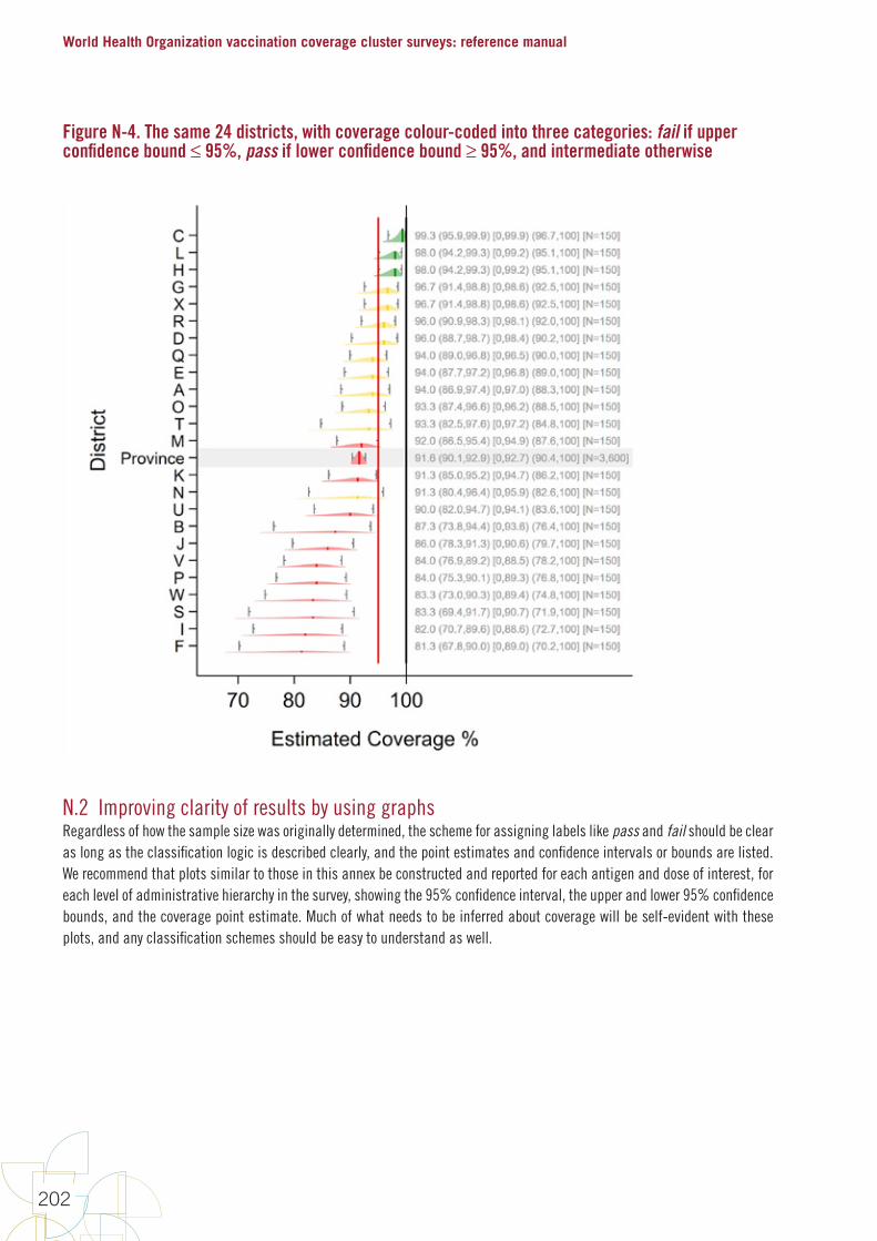
World Health Organization vaccination coverage cluster surveys: reference manual
202
Figure N-4. The same 24 districts, with coverage colour-coded into three categories: fail if upper confidence bound ≤ 95%, pass if lower confidence bound ≥ 95%, and intermediate otherwise
N.2 Improving clarity of results by using graphsRegardless of how the sample size was originally determined, the scheme for assigning labels like pass and fail should be clear as long as the classification logic is described clearly, and the point estimates and confidence intervals or bounds are listed. We recommend that plots similar to those in this annex be constructed and reported for each antigen and dose of interest, for each level of administrative hierarchy in the survey, showing the 95% confidence interval, the upper and lower 95% confidence bounds, and the coverage point estimate. Much of what needs to be inferred about coverage will be self-evident with these plots, and any classification schemes should be easy to understand as well.
Annexes
203
Annex O: Missed opportunities for vaccination (MOV) analysis
O.1 IntroductionA broad variety of authors in the peer-reviewed literature have calculated reasonable and logical measures for missed opportunities for vaccination (MOV) based on survey datasets. As far as we are aware, however, there is no definitive guide or consensus document regarding which measures are clearest and most helpful to EPI programme managers.
Some measures are likely to be better than others for specific purposes. This annex provides some details and worked examples of MOV analysis, working through vaccination records for five children and precisely calculating the numerators and denominators for the measures suggested here. Furthermore, this annex illustrates that the calculations are complicated by how one addresses the topic of doses administered too early (either before the minimum age of eligibility or before the minimum intra-dose interval has elapsed). If the calculations utilize a crude dose analysis and count all doses that are administered, the calculations will yield one set of MOV results. If, instead, a valid dose analysis is conducted and the calculations do not “count” doses that were administered early, children who received early doses will be considered to be under-vaccinated, and as having missed more opportunities for vaccination than would be counted for them in a crude dose analysis. Whether you prefer the crude or valid dose MOV analysis may depend on the main objective of your analysis.
The calculations for the valid dose analysis are substantially more complicated than those for crude doses, so it may suffice to do the crude calculations and then include language in the survey report explaining that the MOV results represent a lower bound, and that higher rates of MOV would likely result from a valid-dose analysis. The document can point to the difference between crude and valid dose coverage, which is calculated as part of the standard coverage survey analysis, to demonstrate the degree to which a crude dose MOV analysis might underestimate what would be obtained in a valid dose analysis.
The WHO tool named Vaccination Coverage Quality Indicators (VCQI) can calculate the MOV indicators described here using either approach: 1) all doses count (crude) when calculating dose eligibility, or 2) only valid doses count, meaning that the child is considered eligible to re-receive doses that were invalid.
O.2 ExamplesTwo examples will be worked through to illustrate an MOV analysis. The first example consists of faux data for five children, and the second example uses actual data from a recent Demographic and Health Survey (DHS).
First, consider the following dates of vaccination for five children in a country whose vaccination schedule is: 1. DTPCV, OPV, and RV (three-dose formulation of RV) beginning at a minimum age of six weeks and with a minimum interval
of four weeks between doses;
2. OPV0 from birth to two weeks and BCG from birth; and
3. MCV1 from age 9 months. Note that in this example, for simplicity, no vaccines were received early (that is, before the child was eligible to receive them) and all vaccines were received before the child was 12 months old.

World Health Organization vaccination coverage cluster surveys: reference manual
204
Table O-1: Dates of vaccination for five children
Child A Child B Child C Child D Child E
Date of birth (d/m/y) 05/05/2012 15/08/2012 20/09/2012 18/07/2012 17/05/2012
From birth BCG 07/05/2012 25/08/2012 19/12/2012 17/04/2013 29/05/2012
From birth to two weeks OPV0 07/05/2012 29/08/2012 29/05/2012
From six weeks
DTPCV1 16/06/2012 26/09/2012 01/11/2012 29/08/2012 06/07/2012
OPV1 16/06/2012 06/10/2012 08/11/2012 29/08/2012 06/07/2012
RV1 16/06/2012 26/09/2012 08/11/2012 29/08/2012 20/07/2012
At least four weeks after previous dose
DTPCV2 16/07/2012 03/11/2012 29/11/2012 26/09/2012 19/08/2012
OPV2 16/07/2012 03/11/2012 29/11/2012 26/09/2012 18/09/2012
RV2 16/07/2012 24/10/2012 29/11/2012 26/09/2012 19/08/2012
At least four weeks after previous dose
DTPCV3 13/08/2012 13/12/2012 20/06/2013 16/09/2012
OPV3 13/08/2012 13/12/2012 20/06/2013 16/10/2012
RV3 13/08/2012 13/12/2012 20/06/2013 16/10/2012
From nine months MCV1 02/02/2013 11/06/2013 17/04/2013 14/02/2013
Fully vaccinated Yes Yes No No Yes
Child A received all vaccines at or close to the recommended age with no MOV. This child had been seen on five separate occasions, none of which resulted in MOV.
Child B had a MOV for OPV0 which could have been given on the same day as BCG, another MOV for OPV1 which could have been given on the same date as DTPCV1 and RV1, and a third MOV for DTPCV2 which could have been given on the same date as RV2. (Note that OPV2 could not have been given on that date because fewer than 28 days had passed since OPV1.) The child had been seen on eight separate occasions, three of which resulted in at least one MOV. All MOVs were corrected by the time of the survey.
Child C had three MOVs for BCG, which could have been given on the same date as DPTCV1, OPV1/RV1, or DPTCV2/OPV2/RV2. There was also an MOV for OPV1 and RV1, which could have been given on the same date as DTPCV1, and another MOV for MCV1, which could have been given on the same date as the third dose of DTPCV, OPV, and RV. The child had still not received MCV1 by the time of the survey (an uncorrected MOV), but all other MOVs were corrected by the time of the survey. The child had been seen on five separate occasions, four of which resulted in at least one MOV. (Note that although the child did not receive OPV0, there had been no opportunity for it because the other vaccines were all given after 14 days of age.)
Child D had two MOVs for BCG, which could have been given at the time of the first or second dose of DTPCV. This child also had an MOV for the third dose of DTPCV, OPV, and RV, which could have been received at the same time as MCV1. The child had not received the latter vaccinations by the time of the survey (an uncorrected MOV). The child had been seen on three separate occasions, all three of which resulted in at least one MOV. (Note that although the child did not receive OPV0, there had been no opportunity for it because the other vaccines were all given after 14 days of age.)
Child E had an MOV for RV1, which could have been received on the same date as DTPCV1 and OPV1; , two MOVs for OPV2, which could have been received on the same date as DTPCV2 or DPTCV3; , and two MOVs for RV3, which could have been received on the same date as DTPCV3 or OPV2. This child had been seen on eight separate occasions, four of which resulted in at least one MOV. All MOVs were corrected by the time of the survey.
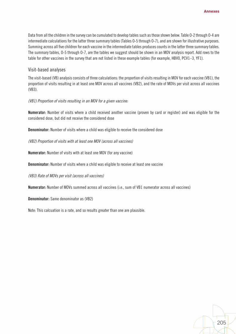
Annexes
205
Data from all the children in the survey can be cumulated to develop tables such as those shown below. Table O-2 through O-4 are intermediate calculations for the latter three summary tables (Tables O-5 through O-7), and are shown for illustrative purposes. Summing across all five children for each vaccine in the intermediate tables produces counts in the latter three summary tables. The summary tables, O-5 through O-7, are the tables we suggest should be shown in an MOV analysis report. Add rows to the table for other vaccines in the survey that are not listed in these example tables (for example, HBV0, PCV1–3, YF1).
Visit-based analyses
The visit-based (VB) analysis consists of three calculations: the proportion of visits resulting in MOV for each vaccine (VB1), the proportion of visits resulting in at least one MOV across all vaccines (VB2), and the rate of MOVs per visit across all vaccines (VB3).
(VB1) Proportion of visits resulting in an MOV for a given vaccine:
Numerator: Number of visits where a child received another vaccine (proven by card or register) and was eligible for the considered dose, but did not receive the considered dose
Denominator: Number of visits where a child was eligible to receive the considered dose
(VB2) Proportion of visits with at least one MOV (across all vaccines)
Numerator: Number of visits with at least one MOV (for any vaccine)
Denominator: Number of visits where a child was eligible to receive at least one vaccine
(VB3) Rate of MOVs per visit (across all vaccines)
Numerator: Number of MOVs summed across all vaccines (i.e., sum of VB1 numerator across all vaccines)
Denominator: Same denominator as (VB2)
Note: This calcuation is a rate, and so results greater than one are plausible.
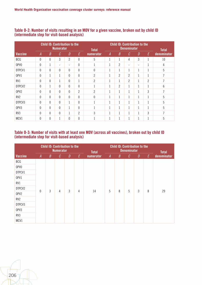
World Health Organization vaccination coverage cluster surveys: reference manual
206
Table O-2: Number of visits resulting in an MOV for a given vaccine, broken out by child ID (intermediate step for visit-based analysis)
Vaccine
Child ID: Contribution to the Numerator Total
numerator
Child ID: Contribution to the Denominator Total
denominatorA B C D E A B C D EBCG 0 0 3 2 0 5 1 1 4 3 1 10
OPV0 0 1 - - 0 1 1 2 - - 1 4
DTPCV1 0 0 0 0 0 0 1 1 1 1 1 5
OPV1 0 1 1 0 0 2 1 2 2 1 1 7
RV1 0 0 1 0 1 2 1 1 2 1 2 7
DTPCV2 0 1 0 0 0 1 1 2 1 1 1 6
OPV2 0 0 0 0 2 2 1 1 1 1 3 7
RV2 0 0 0 0 0 0 1 1 1 1 1 5
DTPCV3 0 0 0 1 0 1 1 1 1 1 1 5
OPV3 0 0 0 1 0 1 1 1 1 1 1 5
RV3 0 0 0 1 2 3 1 1 1 1 3 7
MCV1 0 0 1 0 0 1 1 1 1 1 1 5
Table O-3: Number of visits with at least one MOV (across all vaccines), broken out by child ID (intermediate step for visit-based analysis)
Vaccine
Child ID: Contribution to the Numerator Total
numerator
Child ID: Contribution to the Denominator Total
denominatorA B C D E A B C D EBCG
0 3 4 3 4 14 5 8 5 3 8 29
OPV0
DTPCV1
OPV1
RV1
DTPCV2
OPV2
RV2
DTPCV3
OPV3
RV3
MCV1
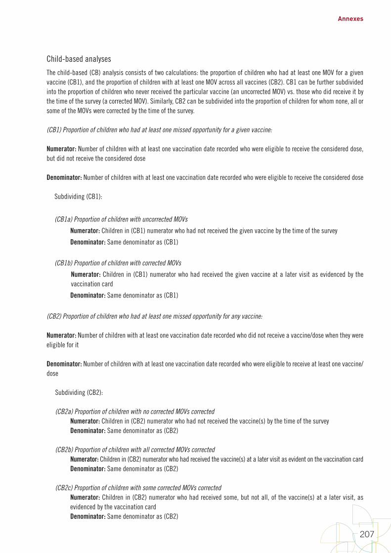
Annexes
207
Child-based analyses
The child-based (CB) analysis consists of two calculations: the proportion of children who had at least one MOV for a given vaccine (CB1), and the proportion of children with at least one MOV across all vaccines (CB2). CB1 can be further subdivided into the proportion of children who never received the particular vaccine (an uncorrected MOV) vs. those who did receive it by the time of the survey (a corrected MOV). Similarly, CB2 can be subdivided into the proportion of children for whom none, all or some of the MOVs were corrected by the time of the survey.
(CB1) Proportion of children who had at least one missed opportunity for a given vaccine:
Numerator: Number of children with at least one vaccination date recorded who were eligible to receive the considered dose, but did not receive the considered dose
Denominator: Number of children with at least one vaccination date recorded who were eligible to receive the considered dose
Subdividing (CB1):
(CB1a) Proportion of children with uncorrected MOVs
Numerator: Children in (CB1) numerator who had not received the given vaccine by the time of the survey
Denominator: Same denominator as (CB1)
(CB1b) Proportion of children with corrected MOVs
Numerator: Children in (CB1) numerator who had received the given vaccine at a later visit as evidenced by the vaccination card
Denominator: Same denominator as (CB1)
(CB2) Proportion of children who had at least one missed opportunity for any vaccine:
Numerator: Number of children with at least one vaccination date recorded who did not receive a vaccine/dose when they were eligible for it
Denominator: Number of children with at least one vaccination date recorded who were eligible to receive at least one vaccine/dose
Subdividing (CB2):
(CB2a) Proportion of children with no corrected MOVs corrected Numerator: Children in (CB2) numerator who had not received the vaccine(s) by the time of the survey Denominator: Same denominator as (CB2)
(CB2b) Proportion of children with all corrected MOVs corrected Numerator: Children in (CB2) numerator who had received the vaccine(s) at a later visit as evident on the vaccination card Denominator: Same denominator as (CB2)
(CB2c) Proportion of children with some corrected MOVs correctedNumerator: Children in (CB2) numerator who had received some, but not all, of the vaccine(s) at a later visit, as evidenced by the vaccination card
Denominator: Same denominator as (CB2)
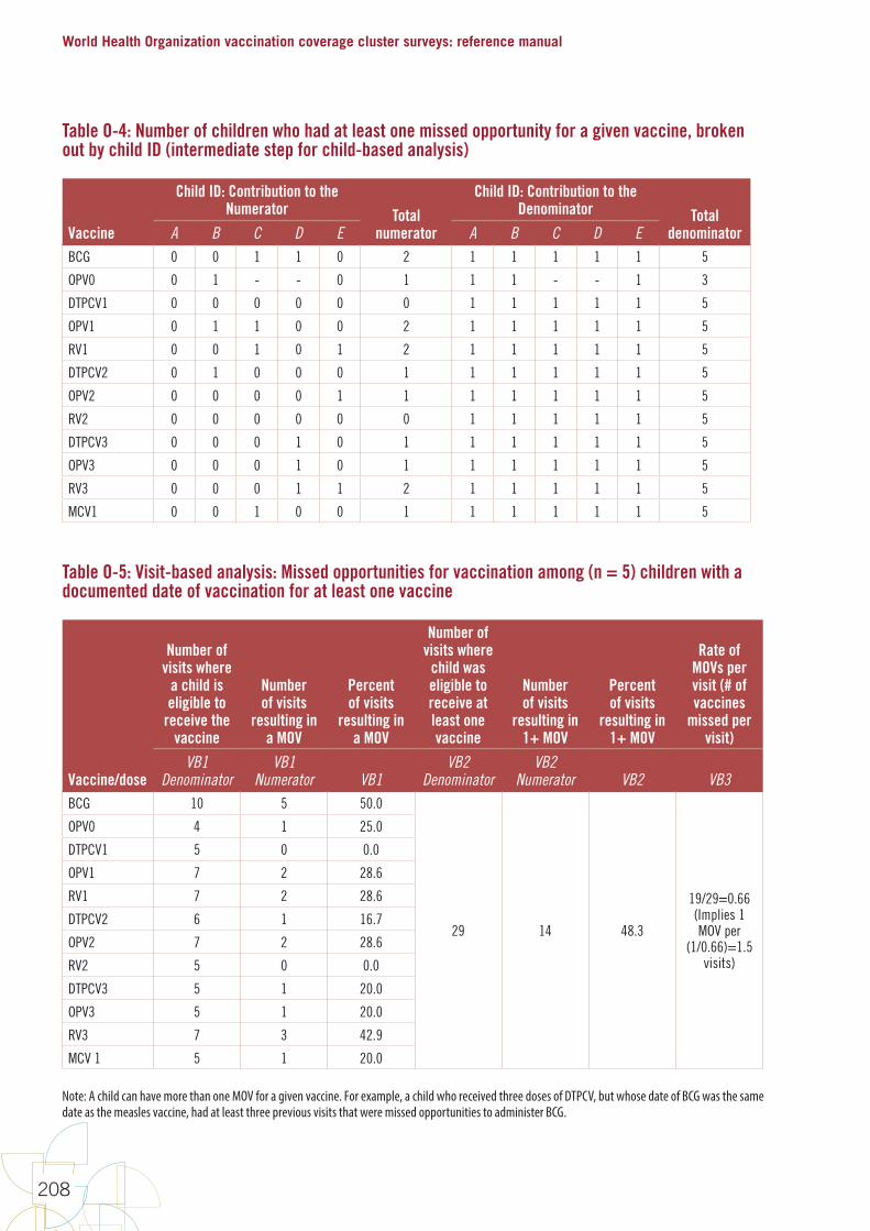
World Health Organization vaccination coverage cluster surveys: reference manual
208
Table O-4: Number of children who had at least one missed opportunity for a given vaccine, broken out by child ID (intermediate step for child-based analysis)
Vaccine
Child ID: Contribution to the Numerator Total
numerator
Child ID: Contribution to the Denominator Total
denominatorA B C D E A B C D EBCG 0 0 1 1 0 2 1 1 1 1 1 5
OPV0 0 1 - - 0 1 1 1 - - 1 3
DTPCV1 0 0 0 0 0 0 1 1 1 1 1 5
OPV1 0 1 1 0 0 2 1 1 1 1 1 5
RV1 0 0 1 0 1 2 1 1 1 1 1 5
DTPCV2 0 1 0 0 0 1 1 1 1 1 1 5
OPV2 0 0 0 0 1 1 1 1 1 1 1 5
RV2 0 0 0 0 0 0 1 1 1 1 1 5
DTPCV3 0 0 0 1 0 1 1 1 1 1 1 5
OPV3 0 0 0 1 0 1 1 1 1 1 1 5
RV3 0 0 0 1 1 2 1 1 1 1 1 5
MCV1 0 0 1 0 0 1 1 1 1 1 1 5
Table O-5: Visit-based analysis: Missed opportunities for vaccination among (n = 5) children with a documented date of vaccination for at least one vaccine
Vaccine/dose
Number of visits where
a child is eligible to
receive the vaccine
Number of visits
resulting in a MOV
Percent of visits
resulting in a MOV
Number of visits where
child was eligible to receive at least one vaccine
Number of visits
resulting in 1+ MOV
Percent of visits
resulting in 1+ MOV
Rate of MOVs per visit (# of vaccines
missed per visit)
VB1 Denominator
VB1 Numerator VB1
VB2 Denominator
VB2 Numerator VB2 VB3
BCG 10 5 50.0
29 14 48.3
19/29=0.66(Implies 1 MOV per
(1/0.66)=1.5 visits)
OPV0 4 1 25.0
DTPCV1 5 0 0.0
OPV1 7 2 28.6
RV1 7 2 28.6
DTPCV2 6 1 16.7
OPV2 7 2 28.6
RV2 5 0 0.0
DTPCV3 5 1 20.0
OPV3 5 1 20.0
RV3 7 3 42.9
MCV 1 5 1 20.0
Note: A child can have more than one MOV for a given vaccine. For example, a child who received three doses of DTPCV, but whose date of BCG was the same date as the measles vaccine, had at least three previous visits that were missed opportunities to administer BCG.
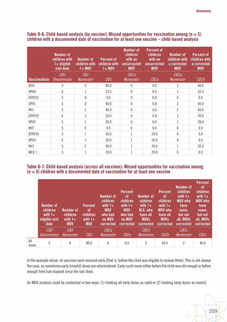
Annexes
209
Table O-6: Child-based analysis (by vaccine): Missed opportunities for vaccination among (n = 5) children with a documented date of vaccination for at least one vaccine – child-based analysis
Vaccine/dose
Number of children with 1+ eligible visit date
Number of children with
1+ MOV
Percent of children with
1+ MOV
Number of children with an
uncorrected MOV
Percent of children with an
uncorrected MOV
Number of children with a corrected
MOV
Percent of children with a corrected
MOV
CB1 Denominator
CB1 Numerator CB1
CB1a Numerator CB1a
CB1b Numerator CB1b
BCG 5 2 40.0 0 0.0 2 40.0
OPV0 3 1 33.3 0 0.0 1 33.3
DTPCV1 5 0 0.0 0 0.0 0 0.0
OPV1 5 2 40.0 0 0.0 2 40.0
RV1 5 2 40.0 0 0.0 2 40.0
DTPCV2 5 1 20.0 0 0.0 1 20.0
OPV2 5 1 20.0 0 0.0 1 20.0
RV2 5 0 0.0 0 0.0 0 0.0
DTPCV3 5 1 20.0 1 20.0 0 0.0
OPV3 5 1 20.0 1 20.0 0 0.0
RV3 5 2 40.0 1 20.0 1 20.0
MCV 1 5 1 20.0 1 20.0 0 0.0
Table O-7: Child-based analysis (across all vaccines): Missed opportunities for vaccination among (n = 5) children with a documented date of vaccination for at least one vaccine
Number of children with 1+
eligible visit date
Number of children with 1+
MOV
Percent of
children with 1+
MOV
Number of children with 1+
MOV who had no MOV
corrected
Percent of
children with 1+
MOV who had no MOV
corrected
Number of children with 1+
M.O. who have all MOVs
corrected
Percent of
children with 1+
MOV who have all MOVs
corrected
Number of children with 1+
MOV who have
some, but not
all, MOVs corrected
Percent of
children with 1+
MOV who have
some, but not
all, MOVs corrected
CB2 Denominator
CB2 Numerator CB2
CB2a Numerator CB2a
CB2b Numerator CB2b
CB2c Numerator CB2c
All doses 5 4 80.0 0 0.0 2 40.0 2 40.0
In the example above, no vaccines were received early (that is, before the child was eligible to receive them). This is not always the case, as sometimes early (invalid) doses are administered. Early could mean either before the child was old enough or before enough time had elapsed since the last dose.
An MOV analysis could be conducted in two ways: (1) treating all early doses as valid or (2) treating early doses as invalid.
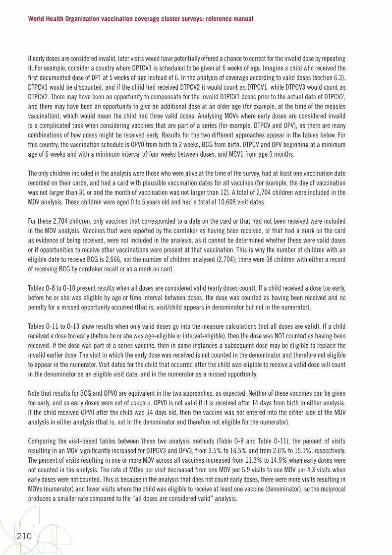
World Health Organization vaccination coverage cluster surveys: reference manual
210
If early doses are considered invalid, later visits would have potentially offered a chance to correct for the invalid dose by repeating it. For example, consider a country where DPTCV1 is scheduled to be given at 6 weeks of age. Imagine a child who received the first documented dose of DPT at 5 weeks of age instead of 6. In the analysis of coverage according to valid doses (section 6.3), DTPCV1 would be discounted, and if the child had received DTPCV2 it would count as DTPCV1, while DTPCV3 would count as DTPCV2. There may have been an opportunity to compensate for the invalid DTPCV1 doses prior to the actual date of DTPCV2, and there may have been an opportunity to give an additional dose at an older age (for example, at the time of the measles vaccination), which would mean the child had three valid doses. Analysing MOVs where early doses are considered invalid is a complicated task when considering vaccines that are part of a series (for example, DTPCV and OPV), as there are many combinations of how doses might be received early. Results for the two different approaches appear in the tables below. For this country, the vaccination schedule is OPV0 from birth to 2 weeks, BCG from birth, DTPCV and OPV beginning at a minimum age of 6 weeks and with a minimum interval of four weeks between doses, and MCV1 from age 9 months.
The only children included in the analysis were those who were alive at the time of the survey, had at least one vaccination date recorded on their cards, and had a card with plausible vaccination dates for all vaccines (for example, the day of vaccination was not larger than 31 or and the month of vaccination was not larger than 12). A total of 2,704 children were included in the MOV analysis. These children were aged 0 to 5 years old and had a total of 10,606 visit dates.
For these 2,704 children, only vaccines that corresponded to a date on the card or that had not been received were included in the MOV analysis. Vaccines that were reported by the caretaker as having been received, or that had a mark on the card as evidence of being received, were not included in the analysis, as it cannot be determined whether these were valid doses or if opportunities to receive other vaccinations were present at that vaccination. This is why the number of children with an eligible date to receive BCG is 2,666, not the number of children analysed (2,704); there were 38 children with either a record of receiving BCG by caretaker recall or as a mark on card.
Tables O-8 to O-10 present results when all doses are considered valid (early doses count). If a child received a dose too early, before he or she was eligible by age or time interval between doses, the dose was counted as having been received and no penalty for a missed opportunity occurred (that is, visit/child appears in denominator but not in the numerator).
Tables O-11 to O-13 show results when only valid doses go into the measure calculations (not all doses are valid). If a child received a dose too early (before he or she was age-eligible or interval-eligible), then the dose was NOT counted as having been received. If the dose was part of a series vaccine, then in some instances a subsequent dose may be eligible to replace the invalid earlier dose. The visit in which the early dose was received is not counted in the denominator and therefore not eligible to appear in the numerator. Visit dates for the child that occurred after the child was eligible to receive a valid dose will count in the denominator as an eligible visit date, and in the numerator as a missed opportunity.
Note that results for BCG and OPV0 are equivalent in the two approaches, as expected. Neither of these vaccines can be given too early, and so early doses were not of concern. OPV0 is not valid if it is received after 14 days from birth in either analysis. If the child received OPV0 after the child was 14 days old, then the vaccine was not entered into the either side of the MOV analysis in either analysis (that is, not in the denominator and therefore not eligible for the numerator).
Comparing the visit-based tables between these two analysis methods (Table O-8 and Table O-11), the percent of visits resulting in an MOV significantly increased for DTPCV3 and OPV3, from 3.5% to 16.5% and from 2.6% to 15.1%, respectively. The percent of visits resulting in one or more MOV across all vaccines increased from 11.3% to 14.9% when early doses were not counted in the analysis. The rate of MOVs per visit decreased from one MOV per 5.9 visits to one MOV per 4.3 visits when early doses were not counted. This is because in the analysis that does not count early doses, there were more visits resulting in MOVs (numerator) and fewer visits where the child was eligible to receive at least one vaccine (denominator), so the reciprocal produces a smaller rate compared to the “all doses are considered valid” analysis.

Annexes
211
In the child-based analysis by vaccine (Table O-9 and Table O-12), these two methods differed considerably in the percent of children with at least one MOV calculation for DTPCV3 and OPV3, from 3.3% to 16.3% and from 2.4% to 14.8%, respectively. The child-based analysis across all vaccines tables (Tables O-10 and O-13) estimated 29.4% of children had at least one MOV when early doses were counted, compared to 36.7% when early doses were not counted. The percent of children with at least one MOV who had no MOVs corrected went from 5.3% to 12.3% when early doses were not counted.
Table O-8: Visit-based analysis: Recent DHS missed opportunities for vaccination among (n = 2,704) children with a documented date of vaccination for at least one vaccine – all doses valid (early doses count)
Vaccine/dose
Number of visits where
a child is eligible to
receive the vaccine
Number of visits
resulting in an MOV
Percent of visits
resulting in an MOV
Number of visits where
child was eligible to receive at least one vaccine
Number of visits
resulting in 1+ MOV
Percent of visits
resulting in 1+ MOV
Rate of MOVs per visit (# of vaccines
missed per visit)
VB1 Denominator
VB1 Numerator VB1 VB2
VB2 Numerator VB2 VB3
BCG 2,798 152 5.4
10,606 1,203 11.3
0.17(Implies 1 MOV per
(1/0.17)=5.9 visits)
OPV0 1,678 39 2.3
DTPCV1 2,978 550 18.5
OPV1 2,932 491 16.7
DTPCV2 2,222 49 2.2
OPV2 2,219 31 1.4
DTPCV3 1,978 70 3.5
OPV3 1,972 51 2.6
MCV 1 1,807 319 17.7
Note: A child can have more than one MOV for a given vaccine. For example, a child who received three doses of DTPCV, but whose date of BCG was the same date as the measles vaccine, had at least three previous visits that were missed opportunities to administer BCG.
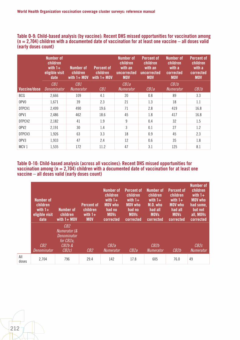
World Health Organization vaccination coverage cluster surveys: reference manual
212
Table O-9: Child-based analysis (by vaccine): Recent DHS missed opportunities for vaccination among (n = 2,704) children with a documented date of vaccination for at least one vaccine – all doses valid (early doses count)
Vaccine/dose
Number of children with 1+
eligible visit date
Number of children
with 1+ MOV
Percent of children
with 1+ MOV
Number of children with an
uncorrected MOV
Percent of children with an
uncorrected MOV
Number of children with a
corrected MOV
Percent of children with a
corrected MOV
CB1 Denominator
CB1 Numerator CB1
CB1a Numerator CB1a
CB1b Numerator CB1b
BCG 2,666 109 4.1 20 0.8 89 3.3
OPV0 1,671 39 2.3 21 1.3 18 1.1
DTPCV1 2,499 490 19.6 71 2.8 419 16.8
OPV1 2,486 462 18.6 45 1.8 417 16.8
DTPCV2 2,182 41 1.9 9 0.4 32 1.5
OPV2 2,191 30 1.4 3 0.1 27 1.2
DTPCV3 1,926 63 3.3 18 0.9 45 2.3
OPV3 1,933 47 2.4 12 0.6 35 1.8
MCV 1 1,535 172 11.2 47 3.1 125 8.1
Table O-10: Child-based analysis (across all vaccines): Recent DHS missed opportunities for vaccination among (n = 2,704) children with a documented date of vaccination for at least one vaccine – all doses valid (early doses count)
Number of children with 1+
eligible visit date
Number of children
with 1+ MOV
Percent of children with 1+
MOV
Number of children with 1+
MOV who had no MOVs
corrected
Percent of children with 1+
MOV who had no MOVs
corrected
Number of children with 1+
M.O. who had all MOVs
corrected
Percent of children with 1+
MOV who had all MOVs
corrected
Number of children with 1+
MOV who had some,
but not all, MOVs corrected
CB2 Denominator
CB2 Numerator (& Denominator
for CB2a, CB2b & CB2c) CB2
CB2a Numerator CB2a
CB2b Numerator CB2b
CB2c Numerator
All doses 2,704 796 29.4 142 17.8 605 76.0 49
Annexes
213
Table O-11: Visit-based analysis: Recent DHS missed opportunities for vaccination among (n = 2,704) children with a documented date of vaccination for at least one vaccine – not all doses valid (early doses DO NOT count)
Vaccine/dose
Number of visits where
a child is eligible to
receive the vaccine
Number of visits
resulting in an MOV
Percent of visits
resulting in an MOV
Number of visits where
child was eligible to receive at least one vaccine
Number of visits
resulting in 1+ MOV
Percent of visits
resulting in 1+ MOV
Rate of MOVs per visit (# of vaccines
missed per visit)
VB1 Denominator
VB1 Numerator VB1 VB2
VB2 Numerator VB2 VB3
BCG 2,798 152 5.4
10,106 1,510 14.9
0.170.23
(Implies 1 MOV per
(1/0.23) = 4.3 visits)
OPV0 1,678 39 2.3
DTPCV1 2,963 562 19.0
OPV1 2,918 503 17.2
DTPCV2 2,187 81 3.7
OPV2 2,167 44 2.0
DTPCV3 1,828 302 16.5
OPV3 1,844 279 15.1
MCV 1 1,599 332 20.8
Note: A child can have more than one MOV for a given vaccine. For example, a child who received three doses of DTPCV, but whose date of BCG was the same date as the measles vaccine, had at least three previous visits that were missed opportunities to administer BCG.
Table O-12 Child-based analysis (by vaccine): Recent DHS missed opportunities for vaccination among (n = 2,704) children with a documented date of vaccination for at least one vaccine – not all doses valid (early doses DO NOT count)
Vaccine/dose
Number of children with 1+
eligible visit date
Number of children
with 1+ MOV
Percent of children
with 1+ MOV
Number of children with an
uncorrected MOV
Percent of children with an
uncorrected MOV
Number of children with a
corrected MOV
Percent of children with a
corrected MOV
CB1 Denominator
CB1 Numerator CB1
CB1a Numerator CB1a
CB1b Numerator CB1b
BCG 2,666 109 4.1 20 0.8 89 3.3
OPV0 1,671 39 2.3 32 1.9 7 0.4
DTPCV1 2,473 502 20.3 72 2.9 430 17.4
OPV1 2,461 473 19.2 46 1.9 427 17.4
DTPCV2 2,134 68 3.2 28 1.3 40 1.9
OPV2 2,143 42 2.0 20 0.9 22 1.0
DTPCV3 1,783 290 16.3 257 14.4 33 1.9
OPV3 1,799 266 14.8 234 13.0 32 1.8
MCV 1 1,326 184 13.9 59 4.4 125 9.4
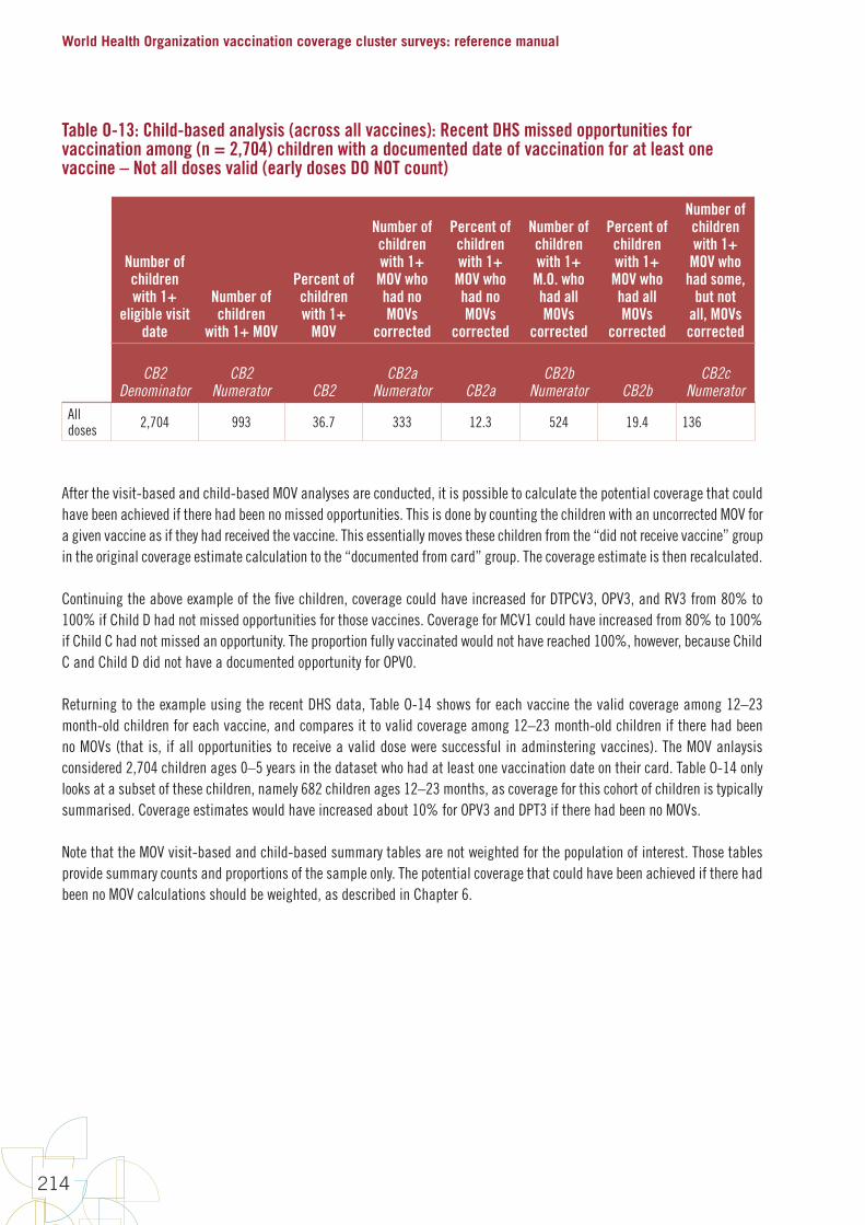
World Health Organization vaccination coverage cluster surveys: reference manual
214
Table O-13: Child-based analysis (across all vaccines): Recent DHS missed opportunities for vaccination among (n = 2,704) children with a documented date of vaccination for at least one vaccine – Not all doses valid (early doses DO NOT count)
Number of children with 1+
eligible visit date
Number of children
with 1+ MOV
Percent of children with 1+
MOV
Number of children with 1+
MOV who had no MOVs
corrected
Percent of children with 1+
MOV who had no MOVs
corrected
Number of children with 1+
M.O. who had all MOVs
corrected
Percent of children with 1+
MOV who had all MOVs
corrected
Number of children with 1+
MOV who had some,
but not all, MOVs corrected
CB2 Denominator
CB2 Numerator CB2
CB2a Numerator CB2a
CB2b Numerator CB2b
CB2c Numerator
All doses 2,704 993 36.7 333 12.3 524 19.4 136
After the visit-based and child-based MOV analyses are conducted, it is possible to calculate the potential coverage that could have been achieved if there had been no missed opportunities. This is done by counting the children with an uncorrected MOV for a given vaccine as if they had received the vaccine. This essentially moves these children from the “did not receive vaccine” group in the original coverage estimate calculation to the “documented from card” group. The coverage estimate is then recalculated.
Continuing the above example of the five children, coverage could have increased for DTPCV3, OPV3, and RV3 from 80% to 100% if Child D had not missed opportunities for those vaccines. Coverage for MCV1 could have increased from 80% to 100% if Child C had not missed an opportunity. The proportion fully vaccinated would not have reached 100%, however, because Child C and Child D did not have a documented opportunity for OPV0.
Returning to the example using the recent DHS data, Table O-14 shows for each vaccine the valid coverage among 12–23 month-old children for each vaccine, and compares it to valid coverage among 12–23 month-old children if there had been no MOVs (that is, if all opportunities to receive a valid dose were successful in adminstering vaccines). The MOV anlaysis considered 2,704 children ages 0–5 years in the dataset who had at least one vaccination date on their card. Table O-14 only looks at a subset of these children, namely 682 children ages 12–23 months, as coverage for this cohort of children is typically summarised. Coverage estimates would have increased about 10% for OPV3 and DPT3 if there had been no MOVs.
Note that the MOV visit-based and child-based summary tables are not weighted for the population of interest. Those tables provide summary counts and proportions of the sample only. The potential coverage that could have been achieved if there had been no MOV calculations should be weighted, as described in Chapter 6.
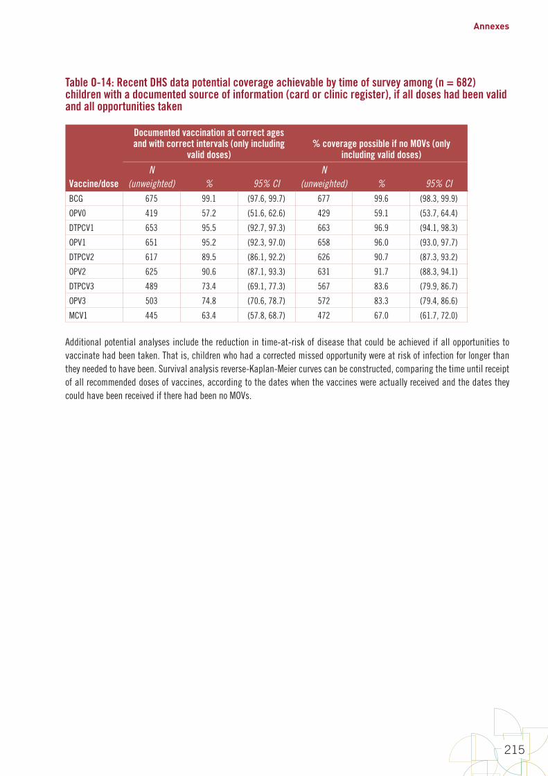
Annexes
215
Table O-14: Recent DHS data potential coverage achievable by time of survey among (n = 682) children with a documented source of information (card or clinic register), if all doses had been valid and all opportunities taken
Vaccine/dose
Documented vaccination at correct ages and with correct intervals (only including
valid doses)% coverage possible if no MOVs (only
including valid doses)
N(unweighted) % 95% CI
N(unweighted) % 95% CI
BCG 675 99.1 (97.6, 99.7) 677 99.6 (98.3, 99.9)
OPV0 419 57.2 (51.6, 62.6) 429 59.1 (53.7, 64.4)
DTPCV1 653 95.5 (92.7, 97.3) 663 96.9 (94.1, 98.3)
OPV1 651 95.2 (92.3, 97.0) 658 96.0 (93.0, 97.7)
DTPCV2 617 89.5 (86.1, 92.2) 626 90.7 (87.3, 93.2)
OPV2 625 90.6 (87.1, 93.3) 631 91.7 (88.3, 94.1)
DTPCV3 489 73.4 (69.1, 77.3) 567 83.6 (79.9, 86.7)
OPV3 503 74.8 (70.6, 78.7) 572 83.3 (79.4, 86.6)
MCV1 445 63.4 (57.8, 68.7) 472 67.0 (61.7, 72.0)
Additional potential analyses include the reduction in time-at-risk of disease that could be achieved if all opportunities to vaccinate had been taken. That is, children who had a corrected missed opportunity were at risk of infection for longer than they needed to have been. Survival analysis reverse-Kaplan-Meier curves can be constructed, comparing the time until receipt of all recommended doses of vaccines, according to the dates when the vaccines were actually received and the dates they could have been received if there had been no MOVs.

World Health Organization vaccination coverage cluster surveys: reference manual
216
Annex P: Suggested outline for coverage survey report
1. High level executive summary
2. Historical background section
a. The EPI (include vaccination schedule(s) that cover all birth cohorts targeted by the survey) and health sector in your country
b. Description of any recent changes in the national immunization programme (for example, the introduction of new vaccines or changes in delivery strategy) or the health sector (for example, introduction of universal health insurance)
c. Summary of recent administrative coverage data or disease outbreak description in the case of a post-SIA survey
d. Summary of previous vaccination coverage survey results
e. Justification for doing this survey
f. Survey objectives (primary, secondary)
3. Survey methods
a. Sampling
i. Target population and exclusions for practical reasons
ii. sampling frames
iii. sample size calculations
iv. Selection methods at each stage
v. Replacement methodology at each stage
b. Profile of implementing personnel
c. Training and piloting
d. Field work (data collection tools, pictures)
e. Ethical considerations
f. Data management (overview of issues related to data collection, segmented clusters with the necessary information, checking, storage and security, etc.)
g. Weighting
i. Overall base weight calculation
ii. Weight adjustments (e.g. nonresponse)
h. Brief summary of the results in terms of sample sizes, response rates, etc. (unweighted or weighted depending on the tables)
i. Final number of clusters (initial, replaced, non-respondent, etc.) by stratum
ii. Final number of households (initial, replaced, non-respondent, etc.) by stratum
iii. Final number of children (initial, replaced, non-respondent, etc.) by stratum
i. Analyses done
4. Results section
a. Summary of available info on those not included in the analysis (for example, refusals, partial completes)
b. Description of sample
i. Summary of respondent background characteristics as appropriate
ii. May want to include issues about estimated number of age-eligible children per household vs. what was observed in each strata/cluster
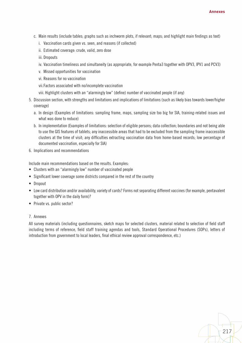
Annexes
217
c. Main results (include tables; graphs such as inchworm plots, if relevant; maps; and highlight main findings as text)
i. Vaccination cards given vs. seen, and reasons (if collected)
ii. Estimated coverage: crude, valid, zero dose
iii. Dropouts
iv. Vaccination timeliness and simultaneity (as appropriate, for example Penta3 together with OPV3, IPV1 and PCV3)
v. Missed opportunities for vaccination
vi. Reasons for no vaccination
vii. Factors associated with no/incomplete vaccination
viii. Highlight clusters with an “alarmingly low” (define) number of vaccinated people (if any)
5. Discussion section, with strengths and limitations and implications of limitations (such as likely bias towards lower/higher coverage)
a. In design (Examples of limitations: sampling frame, maps, sampling size too big for SIA, training-related issues and what was done to reduce)
b. In implementation (Examples of limitations: selection of eligible persons; data collection; boundaries and not being able to use the GIS features of tablets; any inaccessible areas that had to be excluded from the sampling frame inaccessible clusters at the time of visit; any difficulties extracting vaccination data from home-based records; low percentage of documented vaccination, especially for SIA)
6. Implications and recommendations
Include main recommendations based on the results. Examples:• Clusters with an “alarmingly low” number of vaccinated people
• Significant lower coverage some districts compared in the rest of the country
• Dropout
• Low card distribution and/or availability, variety of cards? Forms not separating different vaccines (for example, pentavalent together with OPV in the daily form)?
• Private vs. public sector?
7. Annexes
All survey materials (including questionnaires, sketch maps for selected clusters, material related to selection of field staff including terms of reference, field staff training agendas and tools, Standard Operational Procedures (SOPs), letters of introduction from government to local leaders, final ethical review approval correspondence, etc.)

Notes:. . . . . . . . . . . . . . . . . . . . . . . . . . . . . . . . . . . . . . . . . . . . . . . . . . . . . . . . . . . . . . . . . . . . . . . . . . . . . . . . . . . . . . . . . . . . . . . . . . .
. . . . . . . . . . . . . . . . . . . . . . . . . . . . . . . . . . . . . . . . . . . . . . . . . . . . . . . . . . . . . . . . . . . . . . . . . . . . . . . . . . . . . . . . . . . . . . . . . . .
. . . . . . . . . . . . . . . . . . . . . . . . . . . . . . . . . . . . . . . . . . . . . . . . . . . . . . . . . . . . . . . . . . . . . . . . . . . . . . . . . . . . . . . . . . . . . . . . . . .
. . . . . . . . . . . . . . . . . . . . . . . . . . . . . . . . . . . . . . . . . . . . . . . . . . . . . . . . . . . . . . . . . . . . . . . . . . . . . . . . . . . . . . . . . . . . . . . . . . .
. . . . . . . . . . . . . . . . . . . . . . . . . . . . . . . . . . . . . . . . . . . . . . . . . . . . . . . . . . . . . . . . . . . . . . . . . . . . . . . . . . . . . . . . . . . . . . . . . . .
. . . . . . . . . . . . . . . . . . . . . . . . . . . . . . . . . . . . . . . . . . . . . . . . . . . . . . . . . . . . . . . . . . . . . . . . . . . . . . . . . . . . . . . . . . . . . . . . . . .
. . . . . . . . . . . . . . . . . . . . . . . . . . . . . . . . . . . . . . . . . . . . . . . . . . . . . . . . . . . . . . . . . . . . . . . . . . . . . . . . . . . . . . . . . . . . . . . . . . .
. . . . . . . . . . . . . . . . . . . . . . . . . . . . . . . . . . . . . . . . . . . . . . . . . . . . . . . . . . . . . . . . . . . . . . . . . . . . . . . . . . . . . . . . . . . . . . . . . . .
. . . . . . . . . . . . . . . . . . . . . . . . . . . . . . . . . . . . . . . . . . . . . . . . . . . . . . . . . . . . . . . . . . . . . . . . . . . . . . . . . . . . . . . . . . . . . . . . . . .
. . . . . . . . . . . . . . . . . . . . . . . . . . . . . . . . . . . . . . . . . . . . . . . . . . . . . . . . . . . . . . . . . . . . . . . . . . . . . . . . . . . . . . . . . . . . . . . . . . .
. . . . . . . . . . . . . . . . . . . . . . . . . . . . . . . . . . . . . . . . . . . . . . . . . . . . . . . . . . . . . . . . . . . . . . . . . . . . . . . . . . . . . . . . . . . . . . . . . . .
. . . . . . . . . . . . . . . . . . . . . . . . . . . . . . . . . . . . . . . . . . . . . . . . . . . . . . . . . . . . . . . . . . . . . . . . . . . . . . . . . . . . . . . . . . . . . . . . . . .
. . . . . . . . . . . . . . . . . . . . . . . . . . . . . . . . . . . . . . . . . . . . . . . . . . . . . . . . . . . . . . . . . . . . . . . . . . . . . . . . . . . . . . . . . . . . . . . . . . .
. . . . . . . . . . . . . . . . . . . . . . . . . . . . . . . . . . . . . . . . . . . . . . . . . . . . . . . . . . . . . . . . . . . . . . . . . . . . . . . . . . . . . . . . . . . . . . . . . . .
. . . . . . . . . . . . . . . . . . . . . . . . . . . . . . . . . . . . . . . . . . . . . . . . . . . . . . . . . . . . . . . . . . . . . . . . . . . . . . . . . . . . . . . . . . . . . . . . . . .
. . . . . . . . . . . . . . . . . . . . . . . . . . . . . . . . . . . . . . . . . . . . . . . . . . . . . . . . . . . . . . . . . . . . . . . . . . . . . . . . . . . . . . . . . . . . . . . . . . .
. . . . . . . . . . . . . . . . . . . . . . . . . . . . . . . . . . . . . . . . . . . . . . . . . . . . . . . . . . . . . . . . . . . . . . . . . . . . . . . . . . . . . . . . . . . . . . . . . . .

WORLD HEALTH ORGANIZATION VACCINATION COVERAGE CLUSTER
SURVEYS: REFERENCE MANUAL