4–1

UWarwick

World Models

4–2

UWarwick

Introduction 1

Structure

Observations: cosmological principle holds: The

universe is homogeneous and isotropic.

=⇒Need theoretical framework obeying the

cosmological principle.

Use combination of• General Relativity

• Thermodynamics

• Quantum Mechanics=⇒ Complicated!

For 99% of the work, the above points can be

dealt with separately:1. Define metric obeying cosmological

principle.

2. Obtain equation for evolution of universe

using Einstein field equations.

3. Use thermo/QM to obtain equation of state.

4. Solve equations.

4–3

UWarwick

FRW Metric 1

GRT vs. Newton

Before we can start to think about universe: Brief

introduction to assumptions of general relativity.=⇒ See theory lectures for the gory details, or check with theliterature (Weinberg or MTW).

Assumptions of GRT:

• Space is 4-dimensional, might be curved

• Matter (=Energy) modifies space (Einstein

field equation).

• Covariance: physical laws must be formulated

in a coordinate-system independent way.

• Strong equivalence principle: There is no

experiment by which one can distinguish

between free falling coordinate systems and

inertial systems.

• At each point, space is locally Minkowski (i.e.,

locally, SRT holds).

=⇒Understanding of geometry of space

necessary to understand physics.

4–4

UWarwick

FRW Metric 2

2D Metrics

Before describing the 4D geometry of the

universe: first look at two-dimensional spaces

(easier to visualize).

After Silk (1997, p. 107)

There are three classes of isotropic and

homogeneous two-dimensional spaces:

• 2-sphere (S 2) positively curved

• x-y-plane (R2) zero curvature

• hyperbolic plane (H 2) negatively curved(curvature ≈∑

angles in triangle >, =, or < 180)

We will now compute what the metric for these

spaces looks like.

4–5

UWarwick

FRW Metric 3

2D Metrics

The metric describes the local geometry of a space.

Differential distance, ds, in Euclidean space, R2:

ds2 = dx21 + dx2

2 (4.1)

The metric tensor, gµν, is defined via

ds2 =∑

µ

∑

ν

gµν dxµ dxν =: gµν dxµ dxν (4.2)

(Einstein’s summation convention)

Thus, for the R2,

g11 = 1 g12 = 0

g21 = 0 g22 = 1(4.3)

But: Other coordinate-systems possible!

Changing to polar coordinates r′, θ, defined by

x1 =: r′ cos θ and x2 =: r′ sin θ (4.4)

r´d

dθθ

θds

dr´

x2

x 1

r´

it is easy to see that

ds2 = dr′2+ r′

2dθ2 (4.5)

substituting r′ = Rr,

(change of scale)

ds2 = Rdr2 + r2 dθ2 (4.6)

4–6

UWarwick

FRW Metric 4

2D Metrics

A more complicated case occurs if space is curved. Easiest

case: surface of three-dimensional sphere (a two-sphere).x3

θ x2

R

x1

θ r´

φ

After Kolb & Turner (1990, Fig. 2.1)

Two-sphere with radius R in R3:

x21 + x2

2 + x23 = R2 (4.7)

Length element of R3:

ds2 = dx21 + dx2

2 + dx23

Eq. (4.7) gives

x3 =√

R2 − x21 − x2

2

such that

dx3 =∂x3

∂x1dx1 +

∂x3

∂x2dx2 = −x1 dx1 + x2 dx2

√

R2 − x21 − x2

2

(4.8)

Introduce again polar coordinates r′, θ in x3-plane:

x1 =: r′ cos θ and x2 =: r′ sin θ (4.4)

(note: r′, θ only unique in upper or lower half-sphere)

The differentials are given by

dx1 = cos θ dr′ − r′ sin θ dθ

dx2 = sin θ dr′ + r′ cos θ dθ(4.9)

4–7

UWarwick

FRW Metric 5

2D Metrics

In cartesian coordinates, the length element on S2 is

ds2 = dx21 + dx2

2 +(x1 dx1 + x2 dx2)

2

R2 − x21 − x2

2

(4.10)

inserting eq. (4.9) gives after some algebra

= r′2

dθ2 +R2

R2 − r′2dr′

2(4.11)

finally, defining r = r′/R (i.e., 0 ≤ r ≤ 1) results in

ds2= R2

dr2

1 − r2+ r2 dθ2

(4.12)

Alternatively, we can work in spherical coordinates on S2

x1 = R sin θ cosφ

x2 = R sin θ sinφ

x3 = R cos θ

(4.13)

(θ ∈ [0, π], φ ∈ [0, 2π]).

Going through the same steps as before, we obtain after

some tedious algebra

ds2 = R2

dθ2 + sin2 θ dφ2

(4.14)

4–8

UWarwick

FRW Metric 6

2D Metrics

(Important) remarks:

1. The 2-sphere has no edges, has no

boundaries, but has still a finite volume,

V = 4πR2.

2. Expansion or contraction of sphere caused by

variation of R =⇒ R determines the scale of

volumes and distances on S 2.

R is called the scale factor

3. Positions on S 2 are defined, e.g., by r and θ,

independent on the value of R

r and θ are called comoving coordinates

4. Although the metrics Eq. (4.10), (4.12), and

(4.14) look very different, they still describe the

same space =⇒ that’s why physics should be

covariant.

4–9

UWarwick

FRW Metric 7

2D Metrics

The hyperbolic plane, H 2, is defined by

x21 + x2

2 − x23 = −R2 (4.15)

If we work in Minkowski space, where

ds2 = dx21 + dx2

2 − dx23 (4.16)

then

= dx21 + dx2

2 −(x1 dx1 + x2 dx2)

2

R2 + x21 + x2

2

(4.17)

=⇒substitute R → iR (where i =√−1) to

obtain same form as for sphere (eq. 4.11)!

Therefore,

ds2 = R2

dr2

1 + r2+ r2 dθ2

(4.18)

4–10

UWarwick

FRW Metric 8

2D Metrics

The analogy to spherical coordinates on the

hyperbolic plane are given by

x1 = R sinh θ cosφ

x2 = R sinh θ sinφ

x3 = R cosh θ

(4.19)

(θ ∈ [−∞,+∞], φ ∈ [0, 2π]).

A session with Maple (see handout) will convince

you that these coordinates give

ds2 = R2

dθ2 + sinh2 θ dφ2

(4.20)

Remark:

H 2 is unbound and has an infinite volume.

4–10

Transcript of Maple session to obtain Eq. (4.20):

4–11

UWarwick

FRW Metric 9

2D Metrics

To summarize:

Sphere:

ds2 = R2

dr2

1 − r2+ r2 dθ2

(4.12)

Plane:

ds2 = R2

dr2 + r2 dθ2

(4.6)

Hyperbolic Plane:

ds2 = R2

dr2

1 + r2+ r2 dθ2

(4.18)

=⇒ All three metrics can be written as

ds2 = R2

dr2

1 − k r2+ r2 dθ2

(4.21)

where k defines the geometry:

k =

+1 spherical

0 planar

−1 hyperbolic

(4.22)

4–12

UWarwick

FRW Metric 10

2D Metrics

For “spherical coordinates” we found:

Sphere:

ds2 = R2

dθ2 + sin2 θ dφ2

(4.14)

Plane:

ds2 = R2

dθ2 + θ2dφ2

(4.6)

Hyperbolic plane:

ds2 = R2

dθ2 + sinh2 θ dφ2

(4.20)

=⇒ All three metrics can be written as

ds2 = R2

dθ2 + S2k(θ) dφ2

(4.23)

where

Sk(θ) =

sin θ for k = +1

θ for k = 0

sinh θ for k = −1

(4.24)

We will also need the cos-like analogue

Ck(θ) =√

1 − kS2k(θ) =

cos θ for k = +1

1 for k = 0

cosh θ for k = −1

(4.25)

Note that, compared to the earlier formulae, some coordinateshave been renamed. This is confusing, but legal. . .

4–13

UWarwick

FRW Metric 11

RW Metric

• Cosmological principle + expansion =⇒∃ freely expanding cosmical coordinate

system.

– Observers =: fundamental observers

– Time =: cosmic timeThis is the coordinate system in which the 3K radiation isisotropic, clocks can be synchronized, e.g., by adjusting time tothe local density of the universe.

=⇒ Metric has temporal and spatial part.This also follows directly from the equivalence principle.

• Homogeneity and isotropy =⇒ spatial part is

spherically symmetric:

dψ2 := dθ2 + sin2 θ dφ2 (4.26)

• Expansion: ∃ scale factor, R(t) =⇒ measure

distances using comoving coordinates.

=⇒ metric looks like

ds2 = c2 dt2 −R2(t)[f2(r) dr2 + g2(r) dψ2

]

(4.27)

where f(r) and g(r) are arbitrary.

4–14

UWarwick

FRW Metric 12

RW Metric

Metrics of the form of eq. (4.27) are called

Robertson-Walker (RW) metrics (1935).Previously studied by Friedmann and Lemaître. . .

One common choice is

ds2 = c2 dt2 −R2(t)[

dr2 + S2k(r) dψ2

] (4.28)

where

R(t): scale factor, containing the physics

t: cosmic time

r, θ, φ: comoving coordinates

Sk(r) was defined in Eq. (4.24).

Remark: θ and φ describe directions on sky, as

seen from the arbitrary center of the

coordinate system (=us), r can be interpreted

as a radial coordinate.

4–15

UWarwick

FRW Metric 13

RW Metric

The RW metric defines an universal coordinate

system tied to expansion of space:

B(x2,y2)

A(x1,y1)

d R(t1)

A(x1,y1)

B(x2,y2)

d R(t2)

Scale factor R(t) describes evolution of

universe.

• d is called the comoving distance.

• D(t) := d ·R(t) is called the proper distance,

(note that R is unitless, i.e., d and dR(t) are measured in Mpc)

“World model”: R(t) from GRT plus assumptions

about physics.

4–16

UWarwick

FRW Metric 14

RW Metric

Other forms of the RW metric are also used:

1. Substitution Sk(r) −→ r gives

ds2 = c2 dt2 − R2(t)

dr2

1 − kr2+ r2 dψ2

(4.29)

(i.e., other definition of comoving radius r).

2. A metric with a dimensionless scale factor,

a(t) :=R(t)

R(t0)=R(t)

R0(4.30)

(where t0=today, i.e., a(t0) = 1), gives

ds2 = c2 dt2 − a2(t)

dr2 +S2k(R0r)

R20

dψ2

(4.31)

3. Using a(t) and the substitution Sk(r) −→ r is also

possible:

ds2 = c2 dt2−a2(t)

dr2

1 − k · (R0r)2+ r2 dψ2

(4.32)

The units of R0r are Mpc =⇒ Used for observations!

4–17

UWarwick

FRW Metric 15

RW Metric

4. Replace cosmic time, t, by conformal time,

dη = dt/R(t) =⇒ conformal metric,

ds2 = R2(η)

dη2 − dr2

1 − kr− r2 dψ2

(4.33)

Theoretical importance of this metric: For k = 0, i.e., a

flat space, the RW metric = Minkowski line element ×R2(η) =⇒ Equivalence principle!

5. Finally, the metric can also be written in the isotropic

form,

ds2 = c2dt2 − R(t)

1 + (k/4)r2

dr2 + r2dψ2

(4.34)

Here, the term in . . . is just the line element of a

3d-sphere =⇒ isotropy!

Note: There are as many notations as authors, e.g., some

use a(t) where we use R(t), etc. =⇒ Be careful!

Note 2: Local homogeneity and isotropy (i.e., within a

Hubble radius, r = c/H0), do not imply global homogeneity

and isotropy =⇒ Cosmologies with a non-trivial topology

are possible (e.g., also with more dimensions. . . ).

4–18

UWarwick

Observational Quantities 1

Hubble’s Law

Hubble’s Law follows from the variation of R(t):

R(t+dt

)r

R(t)r

r r

Small scales =⇒ Euclidean geometry

Proper distance between two observers:

D(t) = d ·R(t) (4.35)

where d: comoving distance.

Expansion =⇒ proper separation changes:

∆D

∆t=R(t + ∆t)d− R(t)d

∆t(4.36)

Thus, for ∆t→ 0,

v =dD

dt= R d =

R

RD =: HD (4.37)

=⇒ Identify local Hubble “constant” as

H =R

R= a(t) (4.38)

(a(t) from Eq. 4.30, a(today) = 1)

Since R = R(t) =⇒H is time-dependent!

For small v, interpreted classically the red-shift is

z = 1 +v

c=⇒ z − 1 =

Hd

c(4.39)

4–19

UWarwick

Observational Quantities 2

Redshift, I

The cosmological redshift is a consequence of

the expansion of the universe:

The comoving distance is constant, thus in terms of the

proper distance:

d =D(t = today)

R(t = today)=D(t)

R(t)= const. (4.40)

Set a(t) = R(t)/R(t = today), then eq. (4.40) implies

λobs =λemit

aemit(4.41)

(λobs: observed wavelength, λemit: emitted wavelength)

Thus the observed redshift is

z =λobs − λemit

λemit=λobs

λemit− 1 (4.42)

or

1 + z =1

aemit=R(t = today)

R(t)(4.43)

Light emitted at z = 1 was emitted when the universe was half asbig as today!

z: measure for relative size of universe at time the observed

light was emitted.

Because of z = νemit/νobs,

νemit

νobs=

1

aemit(4.44)

4–19

An alternative derivation of the cosmological redshift follows directly from general relativity, using the basicGR fact that for photons ds2 = 0. Inserting this into the metric, and assuming without loss of generalitythat dψ2 = 0, one finds

0 = c2 dt2 −R2(t) dr2 =⇒ dr = ± c dt

R(t)(4.45)

Since photons travel forward, we choose the +-sign.

temit

temit+∆ tetobs

tobs+∆ to

The comoving distance traveled by photons emitted at cosmic times temit and temit + ∆te is

r1 =

∫tobs

temit

c dt

R(t)and r2 =

∫tobs+∆to

temit+∆te

c dt

R(t)(4.46)

But the comoving distances are equal, r1 = r2! Therefore

0 =

∫tobs

temit

c dt

R(t)−∫

tobs+∆to

temit+∆te

c dt

R(t)(4.47)

=

∫temit+∆te

temit

c dt

R(t)−∫

tobs+∆to

tobs

c dt

R(t)(4.48)

If ∆t small =⇒ R(t) ≈ const.:

=c ∆teR(temit)

− c ∆toR(tobs)

(4.49)

For a wave: c∆t = λ, such that

λemit

R(temit)=

λobs

R(tobs)⇐⇒ λemit

λobs

=R(temit)

R(tobs)(4.50)

From this equation it is straightforward to derive Eq. (4.42).

4–20

UWarwick

Observational Quantities 3

Redshift, II

Outside of the local universe: Eq. (4.43) only valid

interpretation of z.

=⇒ It is common to interpret z as in special

relativity:

1 + z =

√

1 + v/c

1 − v/cThis is WRONG

(4.51)

Redshift is due to expansion of space, not due to

motion of galaxy.What is true is that z is accumulation of many infinitesimalred-shifts à la Eq. (4.39), see, e.g., Peacock (1999).

4–21

UWarwick

Observational Quantities 4

Time Dilatation

Note the implication of Eq. (4.49) on the hand-out:

c ∆teR(temit)

=c ∆toR(tobs)

(4.49)

=⇒ dt/R is constant:

dt

R(t)= const. (4.52)

In other words:dtobs

dtemit=R(tobs)

R(temit)= 1 + z (4.53)

=⇒ Time dilatation of events at large z.

This cosmological time dilatation has been

observed in the light curves of supernova

outbursts.

All other observables apart from z (e.g., number

density N (z), luminosity distance dL, etc.)

require explicit knowledge of R(t) =⇒ Need to

look at the dynamics of the universe.

4–22

UWarwick

Dynamics 1

Friedmann Equations, I

General relativistic approach: Insert metric into

Einstein equation to obtain differential equation

for R(t):

Einstein equation:

Rµν −1

2Rgµν

︸ ︷︷ ︸

Gµν

=8πG

c4Tµν + Λgµν (4.54)

where

gµν: Metric tensor (ds2 = gµν dxµ dxν)

Rµν: Ricci tensor (function of gµν)

R: Ricci scalar (function of gµν)

Gµν: Einstein tensor (function of gµν)

Tµν: Stress-energy tensor, describing curvature

of space due to fields present (matter,

radiation,. . . )

Λ: Cosmological constant

=⇒Messy, but doable

4–23

UWarwick

Dynamics 2

Friedmann Equations, II

r R(t)

m

M

Here, Newtonian derivation of

Friedmann equations: Dynamics

of a mass element on the

surface of sphere of density ρ(t)

and comoving radius d, i.e.,

proper radius d ·R(t) (after

McCrea & Milne, 1934).

Mass of sphere:

M =4π

3(dR)3ρ(t) =

4π

3d3ρ0 where ρ(t) =

ρ0

R(t)3

(4.55)

Force on mass element:

md2

dt2(

dR(t))

= − GMm

(dR(t))2= −4πG

3

dρ0

R2(t)m (4.56)

Canceling m · d gives momentum equation:

R = −4πG

3

ρ0

R2= −4πG

3ρ(t)R(t) (4.57)

From energy conservation, or from multiplying Eq. (4.57)

with R and integrating, we obtain the energy equation,

1

2R2 = +

4πG

3

ρ0

R(t)+ const.

= +4πG

3ρ(t)R2(t) + const.

(4.58)

where the constant can only be obtained from GR.

4–24

UWarwick

Dynamics 3

Friedmann Equations, III

Problems with the Newtonian derivation:

1. Cloud is implicitly assumed to have rcloud <∞(for rcloud → ∞ the force is undefined)

=⇒ violates cosmological principle.

2. Particles move through space

=⇒ v > c possible

=⇒ violates SRT.

Why do we get correct result?

GRT −→ Newton for small scales and mass

densities; since universe is isotropic =⇒ scale

invariance on Mpc scales =⇒ Newton sufficient

(classical limit of GR).

(In fact, point 1 above does hold in GR: Birkhoff’s theorem).

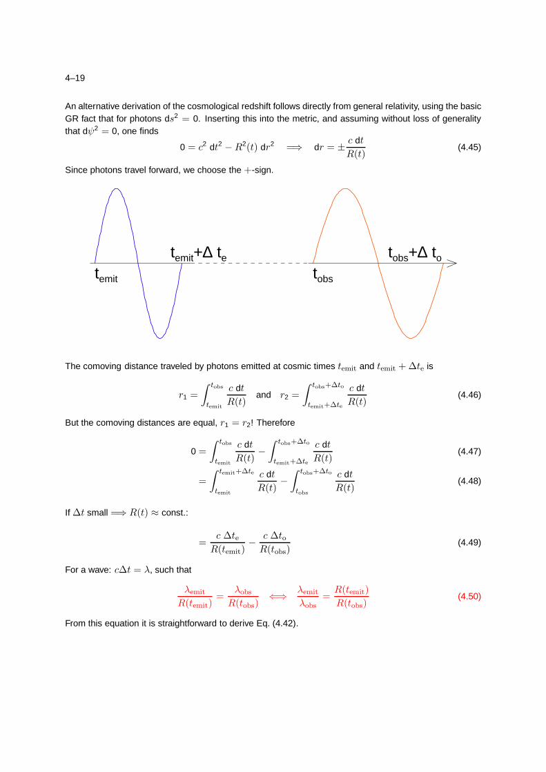
4–25

UWarwick

Dynamics 4

Friedmann Equations, IV

The exact GR derivation of Friedmanns equation

gives:

R = −4πG

3R(

ρ +3p

c2

)

+[1

3ΛR]

R2 = +8πGρ

3R2 − kc2 +

[1

3Λc2R2

] (4.59)

Notes:

1. For k = 0: Eq. (4.59) −→ Eq. (4.58).

2. k ∈ −1, 0,+1 determines the curvature of

space.

3. The density, ρ, includes the contribution of all

different kinds of energy (remember

mass-energy equivalence!).

4. There is energy associated with the vacuum,

parameterized by the parameter Λ.

The evolution of the Hubble parameter is (Λ = 0):

(R

R

)2

= H2(t) =8πGρ

3− kc2

R2(4.60)

4–26

UWarwick

Dynamics 5

The Critical Density, I

Solving Eq. (4.60) for k:

R2

c

(8πG

3ρ−H2

)

= k (4.61)

=⇒Sign of curvature parameter k only depends

on density, ρ:

Defining

ρc =3H2

8πGand Ω =

ρ

ρc(4.62)

it is easy to see that:

Ω > 1 =⇒ k > 0 closed

Ω = 1 =⇒ k = 0 flat

Ω < 1 =⇒ k < 0 open

thus ρc is called the critical density.

For Ω ≤ 1 the universe will expand until ∞,

for Ω > 1 we will see the “big crunch”.

Current value of ρc: ∼ 1.67 × 10−24 g/cm3,

(3. . . 10 H-atoms/m3).

Measured: Ω = 0.1 . . . 0.3.

(but note that Λ can influence things (ΩΛ = 0.7)!).

4–27

UWarwick

Dynamics 6

The Critical Density, II

Ω has a second order effect on the expansion:

Taylor series of R(t) around t = t0:

R(t)

R(t0)=R(t0)

R(t0)+R(t0)

R(t0)(t− t0)+

1

2

R(t0)

R(t0)(t− t0)2

(4.63)

The Friedmann equation Eq. (4.57) can be written

R

R= −4πG

3ρ = −4πG

3Ω

3H2

8πG= −ΩH2

2(4.64)

Since H(t) = R/R (Eq. 4.38), Eq. (4.63) is

R(t)

R(t0)= 1+H0 (t−t0)−

1

2

Ω0

2H2

0 (t−t0)2 (4.65)

where H0 = H(t0) and Ω0 = Ω(t0).The subscript 0 is often omitted in the case of Ω.

Often, Eq. (4.65) is written using the deceleration

parameter:

q :=Ω

2= −R(t0)R(t0)

R2(t0)(4.66)

4–28

UWarwick

Dynamics 7

Equation of state, I

For the evolution of the universe, need to look at

three different kinds of equation of state:

Matter : Normal particles get diluted by expansion

of the universe:

ρm ∝ R−3 (4.67)

Matter is also often called dust by cosmologists.

Radiation : The energy density of radiation

decreases because of volume expansion and

because of the cosmological redshift

(Eq. 4.50: λo/λe = νe/νo = R(to)/R(te)) =⇒ρr ∝ R−4 (4.68)

Vacuum : The vacuum energy density (=Λ) is

independent of R:

ρv = const. (4.69)

Inserting these equations of state into the Friedmann

equation and solving with the boundary condition

R(t = 0) = 0 then gives a specific world model.

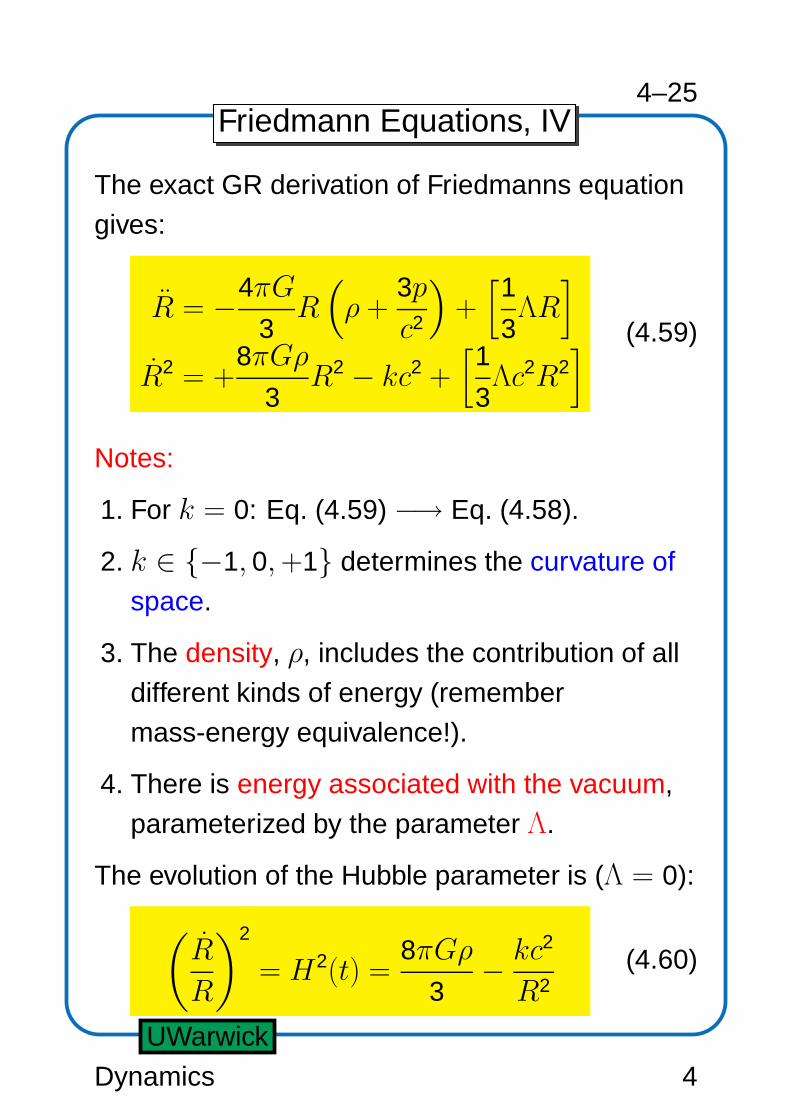
4–29

UWarwick

Dynamics 8

Equation of state, II

Current scale factor is determined by H0 and Ω0:

Friedmann for t = t0:

R20 −

8πG

3ρR2

0 = −kc2 (4.70)

Insert Ω and note H0 = R0/R0

⇐⇒ H20R

20 −H2

0Ω0R20 = −kc2 (4.71)

And therefore

R0 =c

H0

√

k

Ω − 1(4.72)

For Ω −→ 0, R0 −→ c/H0, the Hubble length.

For Ω = 1, R0 is arbitrary.

We now have everything we need to solve the

Friedmann equation and determine the evolution

of the universe. Three cases: k = 0, +1, −1.

4–30

UWarwick

Dynamics 9

k = 0, Matter dominated

For the matter dominated, flat case (the Einstein-de Sitter

case), the Friedmann equation is

R2 − 8πG

3

ρ0R30

R3R2 = 0 (4.73)

For k = 0: Ω = 1 and

8πGρ0

3= Ω0H

20R

30 = H2

0R30 (4.74)

Therefore, the Friedmann eq. is

R2 − H20R

30

R= 0 =⇒ dR

dt= H0R

3/20 R−1/2 (4.75)

Separation of variables and setting R(0) = 0,∫ R(t)

0R1/2 dR = H0R

3/20 t ⇐⇒ 2

3R3/2(t) = H0R

3/20 t

(4.76)

Such that

R(t) = R0

(3H0

2t

)2/3

(4.77)

For k = 0, the universe expands until ∞, its current age

(R(t0) = R0) is given by

t0 =2

3H0(4.78)

Reminder: The Hubble-Time is H−10 = 9.78 Gyr/h.

4–31

UWarwick

Dynamics 10

k = +1, Matter dominated, I

For the matter dominated, closed case, Friedmanns

equation is

R2 − 8πG

3

ρ0R30

R= −c2 ⇐⇒ R2 − H2

0R30Ω0

R= −c2

(4.79)

Inserting R0 from Eq. (4.72) gives

R2 − H20c

3Ω0

H30(Ω − 1)3/2

1

R= −c2 (4.80)

which is equivalent to

dR

dt= c

(ξ

R− 1

)1/2

with ξ =c

H0

Ω0

(Ω0 − 1)3/2(4.81)

With the boundary condition R(0) = 0, separation of

variables gives

ct =

∫ R(t)

0

dR

(ξ/R− 1)1/2=

∫ R(t)

0

√R dR

(ξ − R)1/2(4.82)

Integration by substitution gives

R = ξ sin2 θ

2=ξ

2(1 − cos θ)

=⇒ ct =ξ

2(θ − sin θ) (4.83)

4–32

UWarwick

Dynamics 11

k = +1, Matter dominated, II

1.5 2.0 2.5 3.0 3.5 4.0Ω

4.5

5.0

5.5

6.0

6.5

t 0/h

[Gyr

]

The age of the universe, t0, is obtained by solving

R0 =c

H0(Ω0 − 1)1/2

=ξ

2(1 − cos θ0)=

1

2

c

H0

Ω0

(Ω0 − 1)3/2(1 − cos θ0) (4.84)

(remember Eq. 4.72!). Therefore

cos θ0 =2 − Ω0

Ω0⇐⇒ sin θ0 =

2

Ω0

√

Ω0 − 1 (4.85)

Inserting this into Eq. (4.83) gives

t0 =1

2H0

Ω0

(Ω0 − 1)3/2

[

arccos

(2 − Ω0

Ω0

)

− 2

Ω0

√

Ω0 − 1

]

(4.86)

4–33

UWarwick

Dynamics 12

k = +1, Matter dominated, III

-20 0 20 40 60t-t0 (arbitrary units)

0.0

0.5

1.0

1.5

R(t

)/R

(t0)

Ω=5 Ω=3

Ω=10

Since R is a cyclic function =⇒ The closed universe has a

finite lifetime.

Max. expansion at θ = π, with a maximum scale factor of

Rmax = ξ =c

H0

Ω0

(Ω0 − 1)3/2(4.87)

After that: contraction to the big crunch at θ = 2π.

=⇒ The lifetime of the closed universe is

t =π

H0

Ω0

(Ω0 − 1)3/2(4.88)

4–34

UWarwick

Dynamics 13

k = −1, Matter dominated, I

Finally, the matter dominated, open case. This case is very

similar to the case of k = +1:

For k = −1, the Friedmann equation becomes

dR

dt= c

(ζ

R+ 1

)1/2

(4.89)

where

ζ =c

H0

Ω0

(1 − Ω0)3/2(4.90)

Separation of variables gives after a little bit of algebra

R =ζ

2(cosh θ − 1)

ct =ζ

2(sinh θ − 1)

(4.91)

where the integration was again performed by substitution.

Note: θ here has nothing to do with the coordinate angle θ!

4–35

UWarwick

Dynamics 14

k = −1, Matter dominated, II

0.2 0.4 0.6 0.8Ω

6

7

8

9

10

t 0/h

[Gyr

]

To obtain the age of the universe, note that at the present

time,

cosh θ0 =2 − Ω0

Ω0

sinh θ0 =2

Ω0

√

1 − Ω0

(4.92)

(identical derivation as that leading to Eq. 4.84) such that

t0 =1

2H0

Ω0

(1 − Ω0)3/2·

·

2

Ω0

√

1 − Ω0 − ln

(

2 − Ω0 + 2√

1 − Ω0

Ω0

) (4.93)

4–36

UWarwick

Dynamics 15

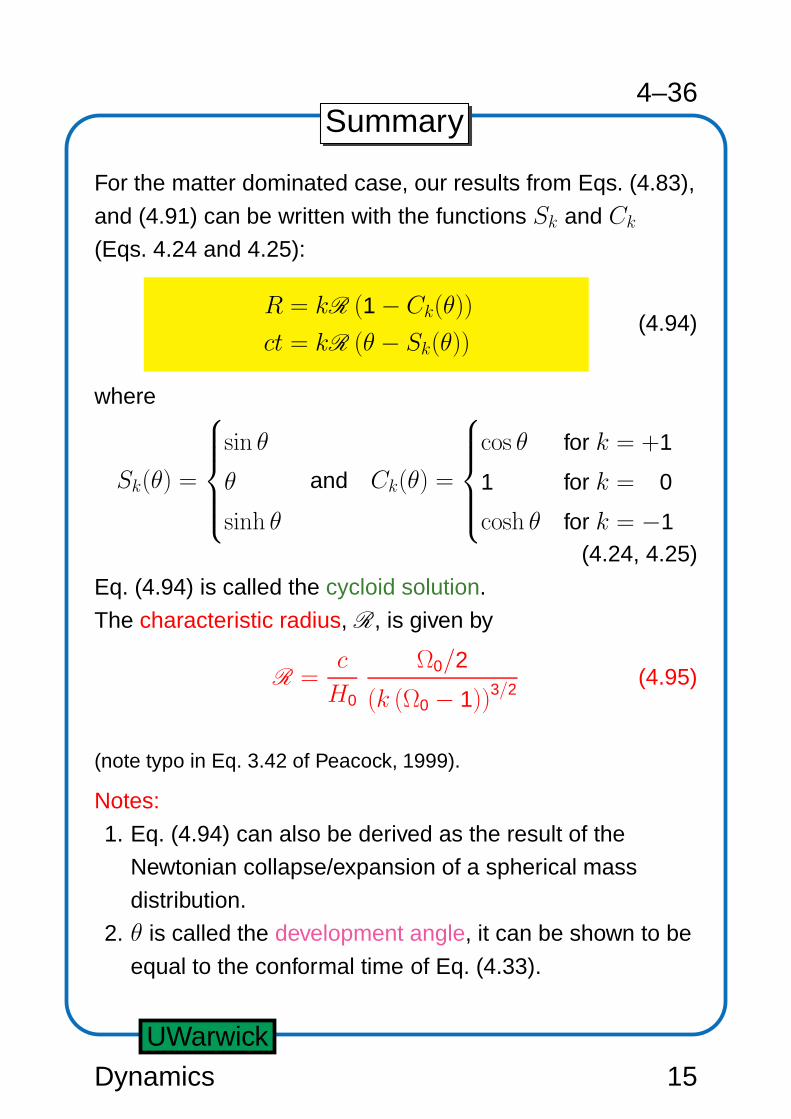
Summary

For the matter dominated case, our results from Eqs. (4.83),

and (4.91) can be written with the functions Sk and Ck(Eqs. 4.24 and 4.25):

R = kR (1 − Ck(θ))

ct = kR (θ − Sk(θ))(4.94)

where

Sk(θ) =

sin θ

θ

sinh θ

and Ck(θ) =

cos θ for k = +1

1 for k = 0

cosh θ for k = −1(4.24, 4.25)

Eq. (4.94) is called the cycloid solution.

The characteristic radius, R, is given by

R =c

H0

Ω0/2

(k (Ω0 − 1))3/2(4.95)

(note typo in Eq. 3.42 of Peacock, 1999).

Notes:

1. Eq. (4.94) can also be derived as the result of the

Newtonian collapse/expansion of a spherical mass

distribution.

2. θ is called the development angle, it can be shown to be

equal to the conformal time of Eq. (4.33).

4–37

UWarwick

Dynamics 16

Summary

0.0 0.5 1.0 1.5ct/2πR

0.1

1.0

10.0

R(t

)/R

k=-1

k= 0

k=+1

BIBLIOGRAPHY 4–37

Bibliography

McCrea, W. H., & Milne, E. A., 1934, Quart. J. Math. (Oxford Series), 5, 73

Silk, J., 1997, A Short History of the Universe, Scientific American Library 53, (New York: W. H. Freeman)