Worldwide Linke turbidity information

HAL Id: hal-00465791https://hal.archives-ouvertes.fr/hal-00465791

Submitted on 21 Mar 2010

HAL is a multi-disciplinary open accessarchive for the deposit and dissemination of sci-entific research documents, whether they are pub-lished or not. The documents may come fromteaching and research institutions in France orabroad, or from public or private research centers.

L’archive ouverte pluridisciplinaire HAL, estdestinée au dépôt et à la diffusion de documentsscientifiques de niveau recherche, publiés ou non,émanant des établissements d’enseignement et derecherche français ou étrangers, des laboratoirespublics ou privés.

Worldwide Linke turbidity informationJan Remund, Lucien Wald, Mireille Lefèvre, Thierry Ranchin, John Page

To cite this version:Jan Remund, Lucien Wald, Mireille Lefèvre, Thierry Ranchin, John Page. Worldwide Linke turbidityinformation. ISES Solar World Congress 2003, Jun 2003, Göteborg, Sweden. 13 p. �hal-00465791�

https://hal.archives-ouvertes.fr/hal-00465791

https://hal.archives-ouvertes.fr

Remund J., Wald L., Lefevre M., Ranchin T., Page J., 2003. Worldwide Linke turbidity information. Proceedings of ISES Solar World Congress, 16-19 June, G�teborg, Sweden, CD-ROM published by International Solar Energy Society.

WORLDWIDE LINKE TURBIDITY INFORMATION

Jan RemundMETEOTEST, Fabrikstrasse 14, CH-3012 Bern, Switzerland,

+41 (0)31 3072626, +41 (0)31 3072610, e-mail: [email protected]

Lucien Wald, Mireille Lefèvre and Thierry RanchinEcole des Mines de Paris /Armines, Groupe Teledetection & Modelisation, BP 207, F-06904 Sophia Antipolis cedex ,

France

John PageEmeritus Professor of University of Sheffield, Building Science, Sheffield S11 9BG, United Kingdom

Abstract – This paper describes the algorithms and data used to construct a worldwide Linke turbidity factor (TL, for an air mass equal to 2)database. Two main steps had to be performed to obtain the information: 1. Assembling estimates of TL and 2. fusing different background layers for the construction of the TL maps. The estimates of TL have two forms: either they stand for specific geographical locations and have a high accuracy, or they are available as gridded data averaged over large areas. Point information was gathered from measured time series of hourly beam and daily global radiation, which were transformed to TL. From publications and networks like AERONET other turbidity quantities were obtained and transformed to TL. The basic gridded data are the maps of daily global irradiation supplied by the NASA-Langley Research Center. The included monthly clear sky irradiations were converted to TL with the same method as for the ground sites. Further gridded information was taken from NOAA pathfinder aerosol data and NASA NVAP. An algorithm was devised to fuse these two types of data and to produce gridded maps in a canonical projection and 5' arc angle cells. These final maps should reproduce the values observed at specific locations. The root mean square error of the interpolation is 0.73 TL units.

1. INTRODUCTION

1.1 The Linke turbidity factorThe Linke turbidity factor (TL, for an air mass equal to

2) is a very convenient approximation to model the atmo-spheric absorption and scattering of the solar radiation under clear skies. It describes the optical thickness of the atmosphere due to both the absorption by the water vapor and the absorption and scattering by the aerosol particles relative to a dry and clean atmosphere. It summarizes the turbidity of the atmosphere, and hence the attenuation of the direct beam solar radiation (WMO, 1981; Kasten, 1996). The larger the TL, the larger the attenuation of the radiation by the clear sky atmosphere.

The direct irradiance on a horizontal surface (or beam horizontal irradiance) for clear sky, Bc, is given by (Rigollier et al. 2000):

mmT RayleighLs ΑΜ2expsinIB 0c

(1)

where I0 is the solar constant, that is the extraterrestrial

irradiance normal to the solar beam at the mean solar distance. It is equal to 1367 Wm-2;

is the correction used to allow for the variation of sun–earth distance from its mean value;

s is the solar altitude angle. s is 0� at sunrise and sunset;

TL(AM2) is the Linke turbidity factor for an air mass equal to 2;

m is the relative optical air mass; m0 the optical air mass at sea level.

Rayleigh (m) is the integrated Rayleigh optical thickness, due to pure molecular scattering.

The pressure correction equation has been newly introduced:

6364.1

0

6364.1

0

1

40

30

200

07995.629578.5750572.0sin1

07995.629578.5750572.0sin

000285.0011517.0

170073.092969.1625928.6

ss

ss

cRayleigh

m

ppm

mm

mmp

(2)

2.8435exp0

zpp (3)

Remund J., Wald L., Lefevre M., Ranchin T., Page J., 2003. Worldwide Linke turbidity information. Proceedings of ISES Solar World Congress, 16-19 June, Göteborg, Sweden, CD-ROM published by International Solar Energy Society.

200

0

200

0

0

000890.003059.068219.1

:5.0

000370.0011997.0248274.1

:75.0

1:

mmp

pp

mmp

pp

Ppp

c

c

c

(4)

Between the pressure levels the correction factor pc is interpolated linearly.

The quantity, exp(-0.8662 TL(AM2) m Rayleigh(m)), represents the beam transmittance of the beam radiation under cloudless skies. The relative optical air mass m expresses the ratio of the optical path length of the solar beam through the atmosphere to the optical path through a standard atmosphere at sea level with the sun at the zenith. As the solar altitude decreases, the relative optical path length increases. The relative optical path length also decreases with increasing station height above the sea level, z.

With the formulation of Grenier (1994) or Rigollier (2000) Rayleigh(m) increases with altitude, because of decreasing air mass m. This error has been eliminated with the new pressure correction pc, adapted to SMART2 (Gueymard, 1998) model output. The new formula corresponds to Gueymards equation at sea level and is very close to the equation of Kasten (1996), used in Rigollier (2000), for sea level altitude.

It is assumed that the integrated optical thickness of the atmosphere is the sum of the integrated optical thicknesses of Rayleigh atmosphere, mixed gases (mainly CO2, O2), ozone, aerosol and water vapor:

wateraerôsolozonegasRayleigh (5)

With this assumption we can write

mms expsinIB 0c

The attenuation caused by the aerosols and the water vapor is known as the turbidity of the atmosphere. The Linke turbidity factor TL is:

RayleighLT

In the past, different types of TL values were used. Grenier (1994) introduced a new formula of Rayleigh optical thickness, which corrected the influence of airmass and led to a lowering of TL of an average of 15 %. We decided to use the original Kasten TL for air mass 2, which is simply:

GrenierTAMT LL 8662.012

For altitude correction of TL the pressure equation is used:

0

0)(ppTzT LL

1.2 MethodologySeveral data sets of the Linke turbidity factor are

available. They are either values for specific geographical sites or are available as gridded data. The values for specific sites are accurate but have a limited extension in space. The gridded values cover the whole world.

The principle is to fuse these two different sets of information in order to obtain the final product on a grid with cells of 5' in size. D'Agostino, Zelenka (1992), Zelenka et al. (1992) and Zelenka, Lazic (1987) proposed solutions to such a problem. In a case similar to ours, since they used the same gridded data, Beyer et al. (1997) proceed as follows: The original gridded data set is resampled by the means of a bicubic spline and re-gridded with a regular cell size of 5' x 5' in a canonical projection. It is then assumed that the value in a cell should be equal to the mean of those observed for the measuring stations within the cell.

For all cells containing at least a measuring station, the difference between both data sets is computed. Then, these differences are interpolated by the means of a linear unbiased interpolator. The authors above-mentioned have employed Kriging or co-Kriging. The distance for interpolation takes into account the orography. Once the field of the residuals is obtained for each cell, this field is added to the gridded data, providing an unbiased gridded map.

The methodology that we used in the construction of our maps of the Linke turbidity factor is derived from that of Beyer et al. (1997). The main drawbacks of the previous method lies in the fact that the gridded data that are fused with the sites observations at cells of 5' in size result from an interpolation of the gridded data at cells of 280 km in size. Accordingly, there are no high frequencies in the gridded data at 5', and more exactly, there are no wavenumbers comprised between 5' and 150' of arc angle.

Therefore, the gridded data is very smooth with the exception of some high frequencies which are locally injected by fusing with sites observations. The method was appropriate in the case of Beyer et al. because a large number of sites observations were available. It is not appropriate in our case however, because large areas are without site observations.

2. DATA

The estimates of the Linke turbidity factor, TL, have two forms: either they stand for specific geographical locations or they are available as gridded data averaged over large areas. The values for specific sites are accurate but have a limited extension in space. The gridded values cover the whole world. They are available for cells of 280 x 280 km2 and are space-averaged.


2.1 Data for specific locationsWe assembled several data sets of the Linke turbidity

factor. They originate from publications and available databases or were derived from measurements of other geophysical parameters. For the latter, the major source is made of measurements of daily global irradiation available for several years. By using the ESRA model for the daily irradiation under clear skies (Rigollier et al. 2000), a technique providing the Linke turbidity factor was developed. Other data are also investigated, such as visibility, Angstr�m coefficients and hourly beam irradiation (Tab. 1).

Tab. 1: Sources of atmospheric turbidity pointinformation

Name of source Abbr. DatabaseHourly beam measurements

B 55 sites with hourly beam measurements

Daily global radi-ation measurements

G 155 sites with daily global radiation measurements

Publications P/A 80 sites with atmospheric turbidity

Angstrom a and b AB ESRA (2000), 595 sitesVisibility (max. per month)

V Globalsod 1996–2000, 1500 sites

Several authors have shown links between visibility and turbidity (King and Buckius, 1971; Gueymard, 2001). But because of bad quality of visibility measurements and the big local influences (horizon) the data could not been taken into account. TL values calculated with Angstrom a and b values had to be discarded as well due to uncertain quality.

Finally, a total of 268 stations was included. All TL's were calculated first at site altitude. In a second step, the values were reduced to sea level with Eqn. 3 in order to be comparable with the background information.

The list of sites and the results are given in the annex.

2.2 Published measurements7 different sources of published data were found. There

are two main groups: One source consists of data of scientific papers (No. 1–6), the other source of published data in the internet (No. 7) (Tab. 2).

Tab. 2: Different sources of published turbidity values

Nr Source N Period1 Gueymard, C.A. and

Garrison J.D. (1998)5 1977–84

2 Gueymard, C. (1994) 14 1971–863 Jacovides, C.P. (1997) 1 1954–924 Pedros, R. et al. (1999) 1 1990–965 Rapti, A.S. (2000) 1 1973–766 B.N.Holben et al. (2000) 23 1993–20007 AERONET Download site

http://aeronet.gsfc.nasa.gov/36 1994–2001

2.3 The gridded dataThe basic gridded data are the maps of daily global

irradiation supplied by the NASA-Langley Research Center, in the framework of the Solar Radiation Budget Project SRB (Whitlock 1995; Di Pasquale, Whitlock 1995).

Using a similar technique as for sites observations, the included monthly clear sky irradiations (Staylor approximation) were converted to Linke turbidity with the same method as for the ground sites with daily global radiation time series. This data set only has a low spatial resolution. The cell is an equal area cell everywhere of 280 x 280 km�. At mid-latitude, it corresponds to approximately 2.5 x 2.5 degrees� of arc angle. The twelve maps (one per month) of TL were re-mapped using the canonical projection. This is performed by the means of the spline bi-cubic operator. A mirror technique is used for the edges. The cells are squared and have a size of 160' of arc angle. This set of worldwide maps is called the set TLSRB.

The Thermal Modeling and Analysis Project (TMAP) at NOAA's Pacific Marine Environmental Laboratory was formed in 1985 to advance understanding of the processes that control the evolution of sea surface temperature and upper ocean thermal structure (TMAP, 2001). The server of this project also provides aerosol optical depth at 630 m for the ocean for several years (1981–00). The aerosol data was transformed to Linke turbidity factor for each cell. Here the equations 16 and 17 were used with water vapour values of NVAP and an assumed of 1.3.

The twelve maps with means of 1985–99 were re-mapped as described above. The cells are square and have a size of 80' of arc angle. Information is only available over the ocean. Comparisons with available measurements over small islands show that this information from TMAP is reliable.

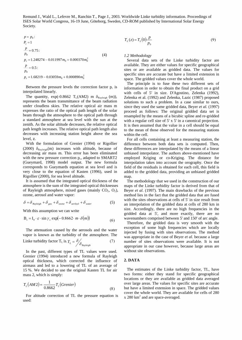
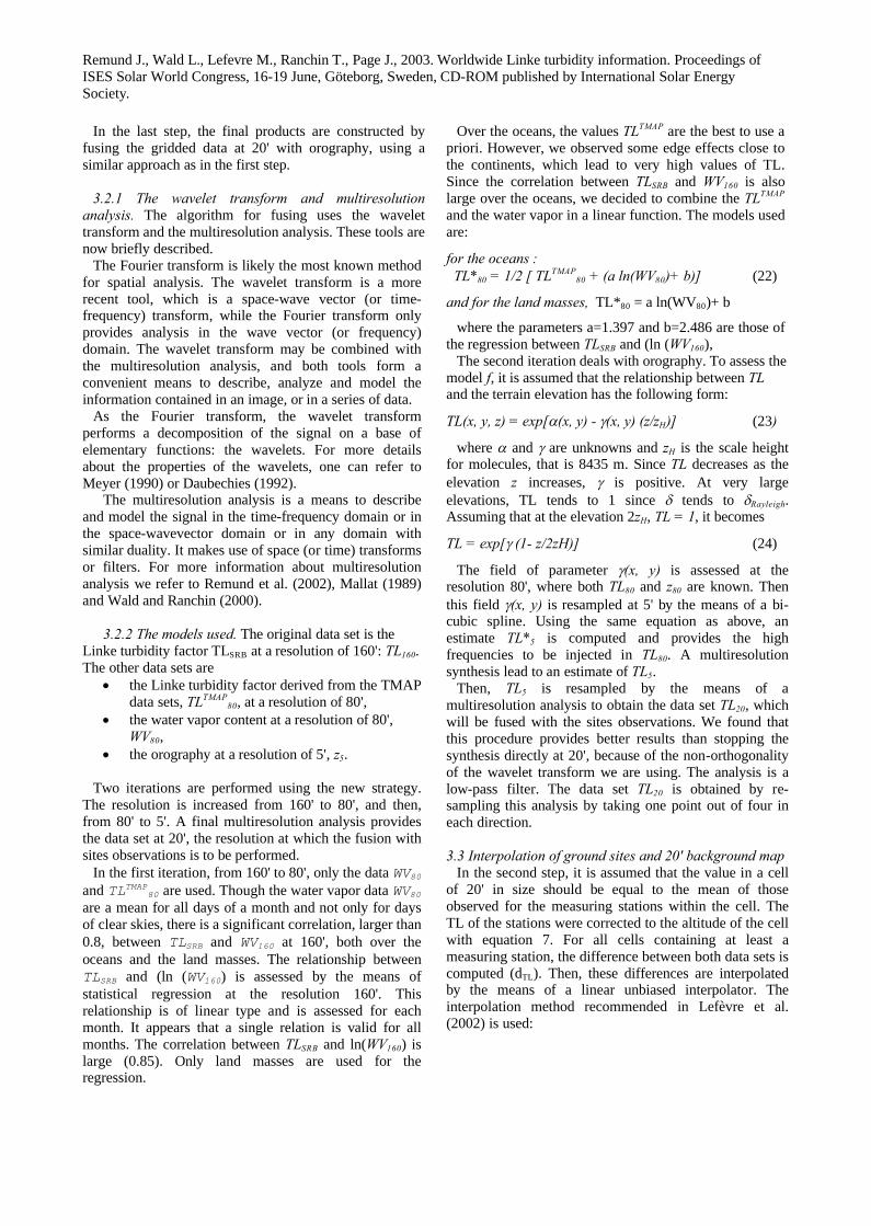
Within the NVAP (NASA Water Vapor Project), the NASA Langley Research Center Atmospheric Sciences Data Center combined several observations to construct world-wide maps of the content of water vapor integrated over the total column (Randel et al., 1996). The gridded data are available on the internet (NVAP, 2001). We computed the mean value for each cell over the 10 years (1988–97) available for each month (Fig. 1). As seen above, the water vapor has an important impact on TL and these data will be used to modulate the field of TL. They are re-mapped as described above. The cells are square and have a size of 80' of arc angle.


Fig. 1: Total water vapor (TPW) according NVAP in cm. January mean (1988–97).

Maps of aerosol index over land and oceans were constructed by the French space agency (CNES) in the framework of the POLDER-ADEOS mission with grid cells of 10' in size. They are available on the internet (CNES, 2001). Unfortunately, only 8 months of data are available (November 1996–June 1997). This source of information was rejected, because of the shortness of this time-series. This impedes an accurate modelling of the high frequencies of the aerosol distribution. Other sources, such as the MODIS/TERRA project, also have short time period and are not used either.

The last set of data that is used in the synthesis is a digital elevation model with a cell size of 5'of arc angle. This model is the TerrainBase model (1995), constructed by the NOAA National Geophysical Data Center. Over the oceans, the elevation was set to 0 m.

3. METHOD

3.1 Method to calculate ground TL values

3.1.1 Method to calculate TL values from beam measurements. The formula (1) was rearranged to determine TL:

mI

B

TRayleigh

s

c

L

8662.0

sinlog

AM2 0

Conditions:

104.0

sin

7.0

1.04.99.04.1exp031.1

sin

W/m200

0

'

'

0

2

s

t

s

ht

t

tt

s

ht

n

KI

GK

k

mkk

IGk

B

All equations for the solar path are taken from ESRA handbook (ESRA, 2000). Several conditions have been used in order not to get beam values influenced by clouds. Without sunshine data it is posteriori very difficult to filter all partially cloudy hours.

According Pedros et al. (1999) only hourly values are used with a sun angle corrected clearness value (kt') of at least 0.7. Additionally, only hours of days with at least 40% of clear hours and a daily clearness index of at least 0.4 are taken into account.

According Gueymard (1998) it is tested if there are jumps between two adjectant hours. If a value is more than 0.5 units higher than the one the hour before, the value is not taken into account. All hourly values higher than the daily median plus 1 unit are cleared. As monthly value the median of all TL values of a month is taken, because the median value is more robust in respect to outliers. Most often the median value is slightly lower than the mean value.

All values were visually checked. Unreasonable data was flagged and not used.

3.1.2 Method to calculate TL values from daily global radiation measurements. With longer time series of daily mean global radiation and ESRA clear sky model (Rigollier, 2000) it is possible to estimate the Linke turbidity. With an iteration of the ESRA clear sky model (daily integration) TL is estimated. TL is varied until the calculated global radation value corresponds to the measured value. This is made for the typical day per month for maximum solar radiation.

Two changes were introduced to the model:1. The new formulation of the Rayleigh optical depth

with altitude (Eqns. 2–4) is used.2. In ESRA (2000) the diffuse formulation did not

make an allowance for variations in the site atmospheric pressure as was the case for the beam estimates. Further investigation has shown the desirability of including the pressure correction. Setting (TL

*) = p/po TL

*0 Lrdsdc TTyFID


2*4

*22*

10797.3

100543.3105843.1

L

LLrd

T

TTT

2210 sinsin sssd AAAyF

2**

2

2**1

2**0

0085079.003231.033025.1

011161.0018945.004020.2

0031408.0061581.026463.0

LL

LL

LL

TTA

TTA

TTA

The database with 97% percentile values was compared at Nice and La Rochelle with the 10 years daily values database. The results are very similar to the mean of the highest 6 values out of 10 years. Out of the original 10 sites only 5 sites could be used due to low quality of the data.

Only time series of at least 5 years were considered. First the mean daily maximum clearness index for each month was calculated. For daily values it is even more difficult to filter clouds a posteriori than for hourly values. To avoid taking cloudy days into account, the mean of the 6 highest monthly means out of the 10 years are taken (5 out of 9 years, 4 out of 7 years if less than 10 years are available). Additionally, a lower limit of Kt was set, similar to the hourly values (Eqn. 16). This limits were adapted to the height of sun because the Perez correction of kt is not suitable for very low solar altitudes:

'

'

'

4.0

51hsmax46.0

30hsmax158.0

30hsmax

tt

tt

tt

kK

kK

kK

With these filters many sites (mainly high latitude sites during winter) could not be calculated because no clear days per month existed. This method is also not suited for tropical and passat zones, where at least during some months no totally clear days exist.

As a minimum value for TL at sea level the following equation was used, which was adapted to the spectral2 model:

8545.12372.00196.0 2min wwTL [w in cm]

If water vapour was measured, w was estimated with dew point temperature.

dTw 07.0075.0exp w in cm

All values were visually checked. Unreasonable data was flagged and not used.

3.1.3 Method to calculate TL values from published turbidity and aerosol values. The published data often had to be recalculated in order to get TL values. Mostly Angstrom values or aerosol optical depth are published. The following formulae are used:

For TLAM2 with values and precipitable water as input the new equation was made according the spectral2 model:

2

2

0254.03153.0427.15

0203.02425.08494.1AM2

wwwwTL

w in cm

The results are very similar to the output of Dogniaux's (1974) equation for TL, but it is not dependent on airmass and solar altitude. The formula was developed for precipitable water contents between 0.5 and 6 cm, between 0 and 0.26 and equal to 1.3.With aerosol optical depth and as input can be calculated (Angstrom, 1929):

a

If more than one wavelength is available can be calculated with (Gueymard, 1994):

21

12log

log

aa

If only one wavelenght is available, an of 1.3 was assumed.

For AERONET stations, where water vapour is also measured, the wavelenghts of 1020 m and 440 m were used to determine . TL Values bigger than 10 were set equal 10. All of the AERONET measurements were madewith CIMEL sun/sky radiometers.

3.2 Fusion of gridded data We propose an innovative approach in the fusion of

gridded data. The algorithm consists of three steps and takes advantage of two known methods.

In the first step, several gridded data sets which have different spatial resolutions and represent different geophysical parameters are fused in order to construct several approximations of the Linke turbidity factor at increasing spatial resolutions. At the end of the first step, the spatial resolution is 20'.

In the second step, it is assumed that the value in a cell of 20' in size should be equal to the mean of those values observed for the measuring stations within the cell. For all cells containing at least one measuring station, the difference between both data sets is computed. Then, these differences are interpolated by the means of a linear unbiased interpolator. Once the field of the residuals is obtained for each cell, this field is added to the gridded data, providing an unbiased gridded map.


In the last step, the final products are constructed by fusing the gridded data at 20' with orography, using a similar approach as in the first step.

3.2.1 The wavelet transform and multiresolution analysis. The algorithm for fusing uses the wavelet transform and the multiresolution analysis. These tools are now briefly described.

The Fourier transform is likely the most known method for spatial analysis. The wavelet transform is a more recent tool, which is a space-wave vector (or time-frequency) transform, while the Fourier transform only provides analysis in the wave vector (or frequency) domain. The wavelet transform may be combined with the multiresolution analysis, and both tools form a convenient means to describe, analyze and model the information contained in an image, or in a series of data.

As the Fourier transform, the wavelet transform performs a decomposition of the signal on a base of elementary functions: the wavelets. For more details about the properties of the wavelets, one can refer to Meyer (1990) or Daubechies (1992).

The multiresolution analysis is a means to describe and model the signal in the time-frequency domain or in the space-wavevector domain or in any domain with similar duality. It makes use of space (or time) transforms or filters. For more information about multiresolution analysis we refer to Remund et al. (2002), Mallat (1989) and Wald and Ranchin (2000).

3.2.2 The models used. The original data set is the Linke turbidity factor TLSRB at a resolution of 160': TL160. The other data sets are

the Linke turbidity factor derived from the TMAP data sets, TLTMAP

80, at a resolution of 80', the water vapor content at a resolution of 80',

WV80, the orography at a resolution of 5', z5.

Two iterations are performed using the new strategy. The resolution is increased from 160' to 80', and then, from 80' to 5'. A final multiresolution analysis provides the data set at 20', the resolution at which the fusion with sites observations is to be performed.

In the first iteration, from 160' to 80', only the data WV80and TLTMAP80 are used. Though the water vapor data WV80are a mean for all days of a month and not only for days of clear skies, there is a significant correlation, larger than 0.8, between TLSRB and WV160 at 160', both over the oceans and the land masses. The relationship between TLSRB and (ln (WV160) is assessed by the means of statistical regression at the resolution 160'. This relationship is of linear type and is assessed for each month. It appears that a single relation is valid for all months. The correlation between TLSRB and ln(WV160) is large (0.85). Only land masses are used for the regression.

Over the oceans, the values TLTMAP are the best to use a priori. However, we observed some edge effects close to the continents, which lead to very high values of TL. Since the correlation between TLSRB and WV160 is also large over the oceans, we decided to combine the TLTMAP

and the water vapor in a linear function. The models used are:

for the oceans :TL*80 = 1/2 [ TLTMAP

80 + (a ln(WV80)+ b)] (22)

and for the land masses, TL*80 = a ln(WV80)+ b

where the parameters a=1.397 and b=2.486 are those of the regression between TLSRB and (ln (WV160),

The second iteration deals with orography. To assess the model f, it is assumed that the relationship between TLand the terrain elevation has the following form:

TL(x, y, z) = exp[(x, y) - (x, y) (z/zH)] (23)

where and are unknowns and zH is the scale height for molecules, that is 8435 m. Since TL decreases as the elevation z increases, is positive. At very large elevations, TL tends to 1 since tends to Rayleigh. Assuming that at the elevation 2zH, TL = 1, it becomes

TL = exp[ (1 - z/2zH)] (24)

The field of parameter (x, y) is assessed at the resolution 80', where both TL80 and z80 are known. Then this field (x, y) is resampled at 5' by the means of a bi-cubic spline. Using the same equation as above, an estimate TL*5 is computed and provides the high frequencies to be injected in TL80. A multiresolution synthesis lead to an estimate of TL5.

Then, TL5 is resampled by the means of a multiresolution analysis to obtain the data set TL20, which will be fused with the sites observations. We found that this procedure provides better results than stopping the synthesis directly at 20', because of the non-orthogonality of the wavelet transform we are using. The analysis is a low-pass filter. The data set TL20 is obtained by re-sampling this analysis by taking one point out of four in each direction.

3.3 Interpolation of ground sites and 20' background mapIn the second step, it is assumed that the value in a cell

of 20' in size should be equal to the mean of those observed for the measuring stations within the cell. The TL of the stations were corrected to the altitude of the cell with equation 7. For all cells containing at least a measuring station, the difference between both data sets is computed (dTL). Then, these differences are interpolated by the means of a linear unbiased interpolator. The interpolation method recommended in Lefèvre et al. (2002) is used:


2sinsin13.011600for

otherwise0for

with 1

wxd

2112

12

212

222i

2

iTL

NS

NS

i

iii

kiii

iT

fmzz

zzvsf

wRdRd

ww

xdL

25

wi : weight i wk : sum of over all weightsR : search radius (1600 km) v : vertical scale factor (500)s : horizontal distance [km] h1, h2 : altitudes of the sites [km]i: Number of sites (maximum 6)1 , 2: latitudes of the two points

After tests with different ranges, the search radius wasset to 1600. The maximum difference added by the second step was limited to 3 TL units.

Additionally the differences dTL were multiplied with a distance factor in order to avoid jumps at the edges of the interpolation areas:

2

iTT

TT

0.5-min*4.29-expdd

1min0.5For

dd5.0minFor

LL

LL

i

i

δ

δ

min(di): distance to the nearest station

Distances up to 800 km are not changed, distances between 800 and 1600 km are decreased smoothly to zero.

Once the field of the residuals is obtained for each cell, this field is added to the gridded data, providing an unbiased gridded map.

4. RESULTS

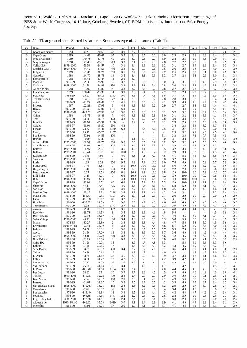
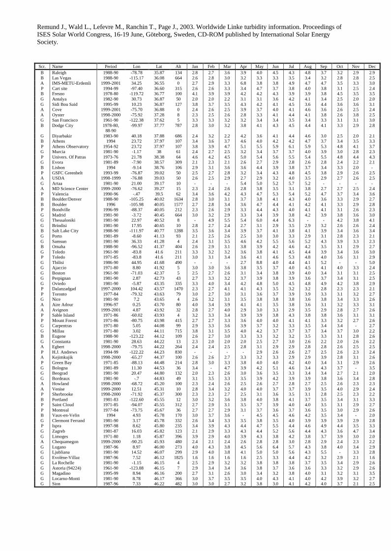
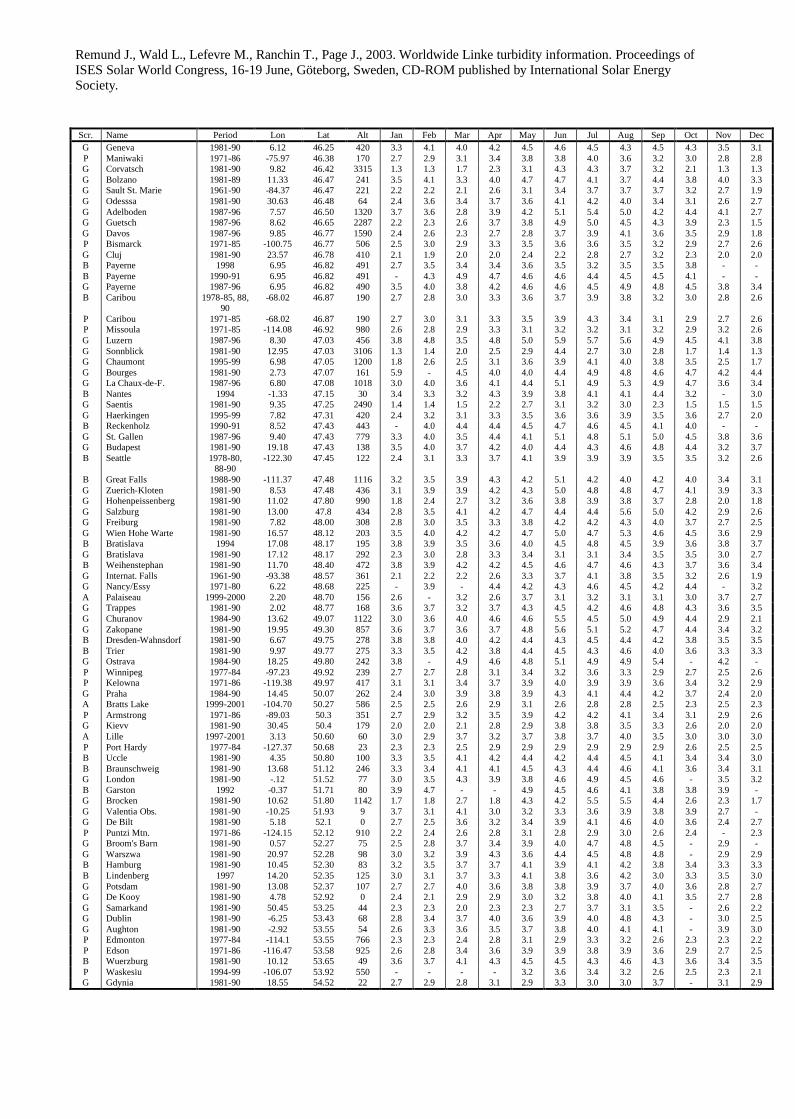
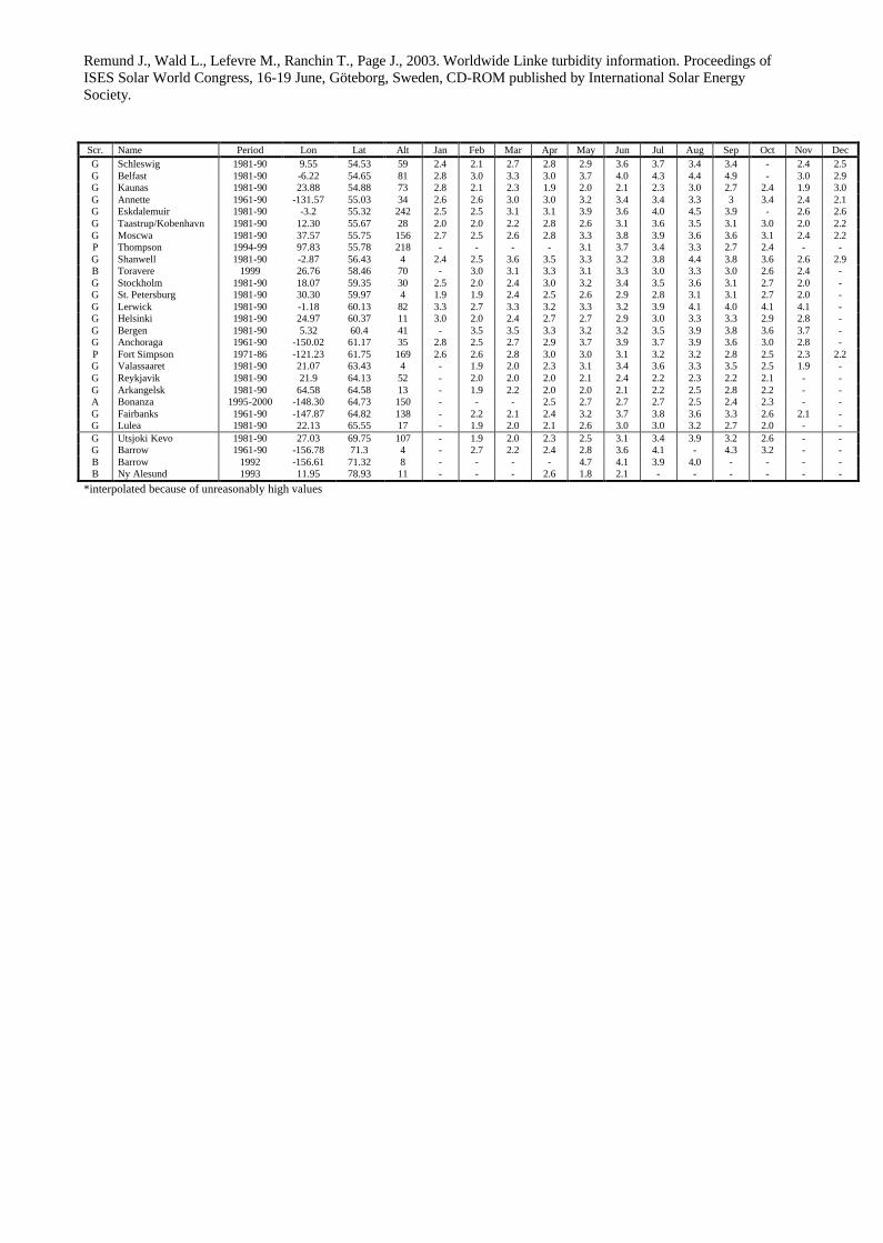
4.1 Ground stationsThe list of measured and calculated ground stations is

given in the Annex Tab. A1. The dataset can be accessed via the prototype of the SoDa project www.soda-is.org.

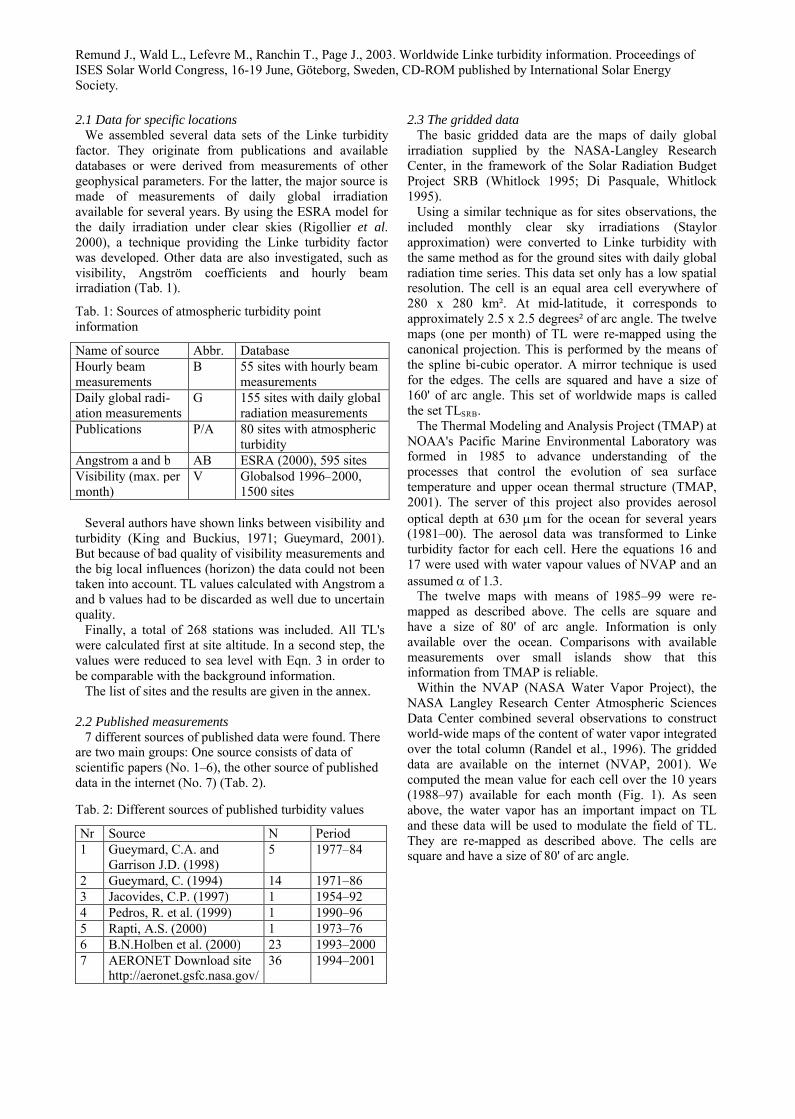
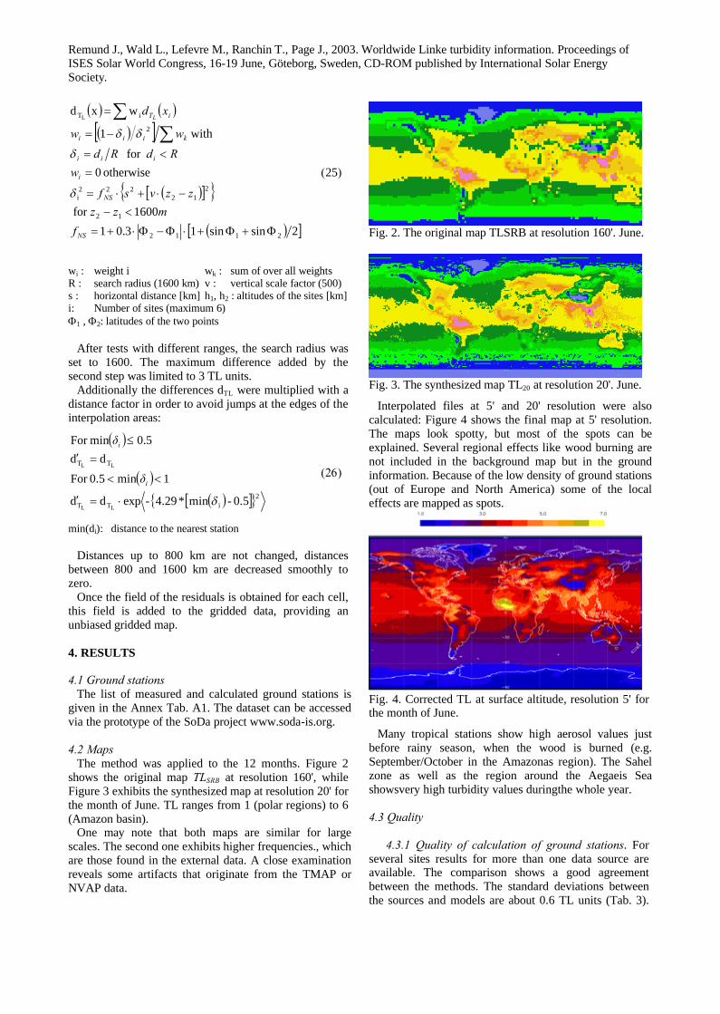
4.2 MapsThe method was applied to the 12 months. Figure 2

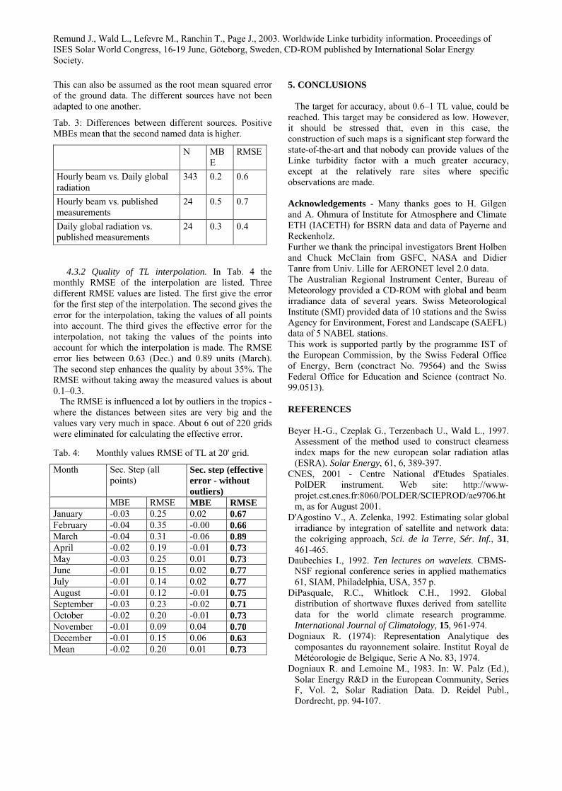
shows the original map TLSRB at resolution 160', while Figure 3 exhibits the synthesized map at resolution 20' for the month of June. TL ranges from 1 (polar regions) to 6 (Amazon basin).

One may note that both maps are similar for large scales. The second one exhibits higher frequencies., which are those found in the external data. A close examination reveals some artifacts that originate from the TMAP or NVAP data.

Fig. 2. The original map TLSRB at resolution 160'. June.

Fig. 3. The synthesized map TL20 at resolution 20'. June.

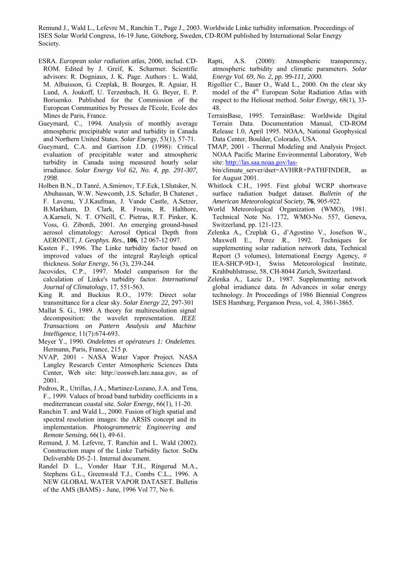
Interpolated files at 5' and 20' resolution were also calculated: Figure 4 shows the final map at 5' resolution. The maps look spotty, but most of the spots can be explained. Several regional effects like wood burning are not included in the background map but in the ground information. Because of the low density of ground stations (out of Europe and North America) some of the local effects are mapped as spots.

Fig. 4. Corrected TL at surface altitude, resolution 5' for the month of June.

Many tropical stations show high aerosol values just before rainy season, when the wood is burned (e.g. September/October in the Amazonas region). The Sahel zone as well as the region around the Aegaeis Sea showsvery high turbidity values duringthe whole year.

4.3 Quality

4.3.1 Quality of calculation of ground stations. For several sites results for more than one data source are available. The comparison shows a good agreement between the methods. The standard deviations between the sources and models are about 0.6 TL units (Tab. 3).


This can also be assumed as the root mean squared error of the ground data. The different sources have not been adapted to one another.

Tab. 3: Differences between different sources. Positive MBEs mean that the second named data is higher.

N MBE

RMSE

Hourly beam vs. Daily global radiation

343 0.2 0.6

Hourly beam vs. published measurements

24 0.5 0.7

Daily global radiation vs. published measurements

24 0.3 0.4

4.3.2 Quality of TL interpolation. In Tab. 4 the monthly RMSE of the interpolation are listed. Three different RMSE values are listed. The first give the error for the first step of the interpolation. The second gives the error for the interpolation, taking the values of all points into account. The third gives the effective error for the interpolation, not taking the values of the points into account for which the interpolation is made. The RMSE error lies between 0.63 (Dec.) and 0.89 units (March). The second step enhances the quality by about 35%. The RMSE without taking away the measured values is about 0.1–0.3.

The RMSE is influenced a lot by outliers in the tropics -where the distances between sites are very big and the values vary very much in space. About 6 out of 220 grids were eliminated for calculating the effective error.

Tab. 4: Monthly values RMSE of TL at 20' grid.

Month Sec. Step (all points)

Sec. step (effective error - without outliers)

MBE RMSE MBE RMSEJanuary -0.03 0.25 0.02 0.67February -0.04 0.35 -0.00 0.66March -0.04 0.31 -0.06 0.89April -0.02 0.19 -0.01 0.73May -0.03 0.25 0.01 0.73June -0.01 0.15 0.02 0.77July -0.01 0.14 0.02 0.77August -0.01 0.12 -0.01 0.75September -0.03 0.23 -0.02 0.71October -0.02 0.20 -0.01 0.73November -0.01 0.09 0.04 0.70December -0.01 0.15 0.06 0.63Mean -0.02 0.20 0.01 0.73

5. CONCLUSIONS

The target for accuracy, about 0.6–1 TL value, could be reached. This target may be considered as low. However, it should be stressed that, even in this case, the construction of such maps is a significant step forward the state-of-the-art and that nobody can provide values of the Linke turbidity factor with a much greater accuracy, except at the relatively rare sites where specific observations are made.

Acknowledgements - Many thanks goes to H. Gilgen and A. Ohmura of Institute for Atmosphere and Climate ETH (IACETH) for BSRN data and data of Payerne and Reckenholz.Further we thank the principal investigators Brent Holben and Chuck McClain from GSFC, NASA and Didier Tanre from Univ. Lille for AERONET level 2.0 data.The Australian Regional Instrument Center, Bureau of Meteorology provided a CD-ROM with global and beam irradiance data of several years. Swiss Meteorological Institute (SMI) provided data of 10 stations and the Swiss Agency for Environment, Forest and Landscape (SAEFL) data of 5 NABEL stations.This work is supported partly by the programme IST of the European Commission, by the Swiss Federal Office of Energy, Bern (conctract No. 79564) and the Swiss Federal Office for Education and Science (contract No. 99.0513).

REFERENCES

Beyer H.-G., Czeplak G., Terzenbach U., Wald L., 1997. Assessment of the method used to construct clearness index maps for the new european solar radiation atlas (ESRA). Solar Energy, 61, 6, 389-397.

CNES, 2001 - Centre National d'Etudes Spatiales. PolDER instrument. Web site: http://www-projet.cst.cnes.fr:8060/POLDER/SCIEPROD/ae9706.htm, as for August 2001.

D'Agostino V., A. Zelenka, 1992. Estimating solar global irradiance by integration of satellite and network data: the cokriging approach, Sci. de la Terre, Sér. Inf., 31, 461-465.

Daubechies I., 1992. Ten lectures on wavelets. CBMS-NSF regional conference series in applied mathematics 61, SIAM, Philadelphia, USA, 357 p.

DiPasquale, R.C., Whitlock C.H., 1992. Global distribution of shortwave fluxes derived from satellite data for the world climate research programme. International Journal of Climatology, 15, 961-974.

Dogniaux R. (1974): Representation Analytique des composantes du rayonnement solaire. Institut Royal de M�t�orologie de Belgique, Serie A No. 83, 1974.

Dogniaux R. and Lemoine M., 1983. In: W. Palz (Ed.), Solar Energy R&D in the European Community, Series F, Vol. 2, Solar Radiation Data. D. Reidel Publ., Dordrecht, pp. 94-107.


ESRA. European solar radiation atlas, 2000, includ. CD-ROM. Edited by J. Greif, K. Scharmer. Scientific advisors: R. Dogniaux, J. K. Page. Authors : L. Wald, M. Albuisson, G. Czeplak, B. Bourges, R. Aguiar, H. Lund, A. Joukoff, U. Terzenbach, H. G. Beyer, E. P. Borisenko. Published for the Commission of the European Communities by Presses de l'Ecole, Ecole des Mines de Paris, France.

Gueymard, C., 1994. Analysis of monthly average atmospheric precipitable water and turbidity in Canada and Northern United States. Solar Energy, 53(1), 57-71.

Gueymard, C.A. and Garrison J.D. (1998): Critical evaluation of precipitable water and atmospheric turbidity in Canada using measured hourly solar irradiance. Solar Energy Vol 62, No. 4, pp. 291-307, 1998.

Holben B.N., D.Tanr�, A.Smirnov, T.F.Eck, I.Slutsker, N. Abuhassan, W.W. Newcomb, J.S. Schafer, B Chatenet , F. Lavenu, Y.J.Kaufman, J. Vande Castle, A.Setzer, B.Markham, D. Clark, R. Frouin, R. Halthore, A.Karneli, N. T. O'Neill, C. Pietras, R.T. Pinker, K. Voss, G. Zibordi, 2001. An emerging ground-based aerosol climatology: Aerosol Optical Depth from AERONET, J. Geophys. Res., 106, 12 067-12 097.

Kasten F., 1996. The Linke turbidity factor based on improved values of the integral Rayleigh optical thickness. Solar Energy, 56 (3), 239-244.

Jacovides, C.P., 1997. Model camparison for the calculation of Linke's turbidity factor. International Journal of Climatology, 17, 551-563.

King R. and Buckius R.O., 1979: Direct solar transmittance for a clear sky. Solar Energy 22, 297-301

Mallat S. G., 1989. A theory for multiresolution signal decomposition: the wavelet representation. IEEE Transactions on Pattern Analysis and Machine Intelligence, 11(7):674-693.

Meyer Y., 1990. Ondelettes et opérateurs 1: Ondelettes. Hermann, Paris, France, 215 p.

NVAP, 2001 - NASA Water Vapor Project. NASA Langley Research Center Atmospheric Sciences Data Center, Web site: http://eosweb.larc.nasa.gov, as of 2001.

Pedros, R., Utrillas, J.A., Martinez-Lozano, J.A. and Tena, F., 1999. Values of broad band turbidity coefficients in a mediterranean coastal site. Solar Energy, 66(1), 11-20.

Ranchin T. and Wald L., 2000. Fusion of high spatial and spectral resolution images: the ARSIS concept and its implementation. Photogrammetric Engineering and Remote Sensing, 66(1), 49-61.

Remund, J. M. Lefevre, T. Ranchin and L. Wald (2002). Construction maps of the Linke Turbidity factor. SoDa Deliverable D5-2-1. Internal document.

Randel D. L., Vonder Haar T.H., Ringerud M.A., Stephens G.L., Greenwald T.J., Combs C.L., 1996. A NEW GLOBAL WATER VAPOR DATASET. Bulletin of the AMS (BAMS) - June, 1996 Vol 77, No 6.

Rapti, A.S. (2000): Atmospheric transperency, atmospheric turbidity and climatic parameters. Solar Energy Vol. 69, No. 2, pp. 99-111, 2000.

Rigollier C., Bauer O., Wald L., 2000. On the clear sky model of the 4th European Solar Radiation Atlas with respect to the Heliosat method. Solar Energy, 68(1), 33-48.

TerrainBase, 1995. TerrainBase: Worldwide Digital Terrain Data. Documentation Manual, CD-ROM Release 1.0, April 1995. NOAA, National Geophysical Data Center, Boulder, Colorado, USA.

TMAP, 2001 - Thermal Modeling and Analysis Project. NOAA Pacific Marine Environmental Laboratory, Web site: http://las.saa.noaa.gov/las-bin/climate_server/dset=AVHRR+PATHFINDER, as for August 2001.

Whitlock C.H., 1995. First global WCRP shortwave surface radiation budget dataset. Bulletin of the American Meteorological Society, 76, 905-922.

World Meteorological Organization (WMO), 1981. Technical Note No. 172, WMO-No. 557, Geneva, Switzerland, pp. 121-123.

Zelenka A., Czeplak G., d’Agostino V., Josefson W., Maxwell E., Perez R., 1992. Techniques for supplementing solar radiation network data, Technical Report (3 volumes), International Energy Agency, # IEA-SHCP-9D-1, Swiss Meteorological Institute, Krahbuhlstrasse, 58, CH-8044 Zurich, Switzerland.

Zelenka A., Lazic D., 1987. Supplementing network global irradiance data. In Advances in solar energy technology. In Proceedings of 1986 Biennial Congress ISES Hamburg, Pergamon Press, vol. 4, 3861-3865.


Tab. A1. TL at ground sites. Sorted by latitude. Scr means type of data source (Tab. 1).Scr. Name Period Lon Lat Alt Jan Feb Mar Apr May Jun Jul Aug Sep Oct Nov DecB Georg von Neum. 1993 -8.25 -70.65 42 3.0 2.7 2.6 - - - - - - 2.1 2.0 2.1B Cape Grim 1999 144.68 -40.67 95 3.5 3.4 3.5 3.0 3.0 2.9 2.5 3.1 3.3 3.4 3.1 3.4B Mount Gambier 1999 140.78 -37.73 69 2.9 3.0 2.8 2.7 3.0 2.8 2.5 2.9 3.3 2.9 3.1 3.1B Wagga Wagga 1998 147.45 -35.15 213 3.3 3.1 2.9 2.9 2.8 2.7 2.7 2.8 3.0 3.0 2.9 3.1A Ceilap-BA 1999-2000 -58.50 -34.57 10 3.1 3.4 3.3 3.1 3.2 3.1 2.7 2.9 3.2 3.4 3.2 3.3A Cordoba-CETT 1999-2000 -64.45 -31.52 730 3.2 2.9 2.9 2.6 2.5 2.6 2.4 2.8 2.9 3.0 2.7 3.0B Kalgoorlie 1999 121.45 -30.77 360 3.6 3.4 3.3 2.9 2.7 2.6 2.6 2.8 3.1 3.0 2.9 3.2B Geraldton 1998 114.70 -28.78 34 3.5 3.4 3.3 3.3 3.2 2.7 2.4 2.8 2.9 3.0 3.1 3.4B Florianopolis 1998 -48.48 -27.47 11 2.5 3.0 - - - - - - - 2.4 2.4 2.4G Maputo 1995-99 32.60 -25.97 70 3.7 3.8 3.3 3.5 3.0 3.1 3.1 3.0 4.0 2.9 3.5 3.2A Skukuza 1998-2000 31.58 -24.98 150 3.3 2.9 3.1 3.4 2.8 3.0 3.4 3.2 4.2 3.8 3.5 3.4B Alice Springs 1998 133.90 -23.80 541 3.8 3.2 3.5 3.0 2.8 2.7 2.7 2.8 3.2 3.2 3.2 3.2B Rockhampton 1999 150.47 -23.38 14 3.9 3.6 3.4 3.1 2.7 2.7 2.8 2.9 3.2 3.2 3.2 3.7G Bulawayo 1995-99 28.62 -20.15 1343 5.0 4.9 4.7 4.8 3.8 3.7 3.7 3.9 4.6 5.5 5.4 5.5B Tennant Creek 1998 134.18 -19.63 377 3.6 3.3 3.5 3.2 2.8 2.8 3.0 2.7 3.2 3.4 3.0 3.6P Arica 1998-99 -70.25 -18.47 25 4.1 5.6 5.5 4.3 4.1 3.9 4.0 4.6 4.4 3.9 4.2 4.6B Broome 1997 122.23 -17.95 9 4.4 4.3 3.9 3.2 2.9 2.7 2.7 3.3 3.9 4.4 4.1 4.1G Harare 1995-99 31.02 -17.83 1471 6.3 5.7 - - - - 4.4 3.9 - 4.5 6.1 6.6A Tahiti 1999-2001 -149.61 -17.58 98 3.6 3.3 3.6 3.3 3.1 3.2 3.2 3.1 3.2 3.3 3.4 3.4B Cairns 1998 145.75 -16.88 7 4.0 4.3 3.2 3.8 3.0 3.1 3.2 3.3 3.6 4.1 3.8 3.7G Tete 1995-99 33.58 -16.18 123 3.8 3.3 2.9 2.8 2.8 3.0 3.3 3.7 5.3 4.1 4.3 3.0P Brasilia 1993-95 -47.90 -15.92 1100 - 3.2 - 3.1 3.1 2.9 2.9 3.8 5.6 4.6 3.8 3.9P Cuiaba 1995-97 -56.00 -15.50 250 4.3 - - - - 3.8 3.8 6.4 8.2 5.7 5.5 -G Lusaka 1995-99 28.32 -15.42 1280 6.3 - 6.3 5.0 2.5 3.1 2.7 3.6 4.9 7.0 5.8 4.4P Mongu 1995-98 23.15 -15.25 1107 - - - - - 2.9 3.2 4.1 4.9 4.5 4.1 3.4P Los Fierros 1998-99 -60.92 -14.55 170 - - - - 3.1 3.3 3.4 7.2 7.7 7.5 4.5 -B Darwin 1999 130.87 -12.40 30 - 4.1 4.0 3.5 3.0 3.1 3.3 3.6 4.4 4.5 4.3 4.0P Abracos Hill 1999-2000 -62.35 -10.75 200 3.3 3.6 3.5 3.2 3.2 3.2 3.2 4.2 5.8 5.9 4.0 3.9P Alta Floresta 1993-95 -56.00 -9.92 175 3.5 3.4 3.6 3.3 3.2 3.2 3.3 7.5 10.0 6.2 - -A Belterra 1999-2001 -54.95 -2.63 70 3.5 4.2 4.4 - 3.5 3.2 3.4 3.8 4.2 5.0 5.0 5.1A Balbina 1999-2001 -59.49 -1.92 80 10.0 3.6 4.5 3.2 3.2 2.9 3.0 3.3 3.6 4.5 4.1 4.4A Kaashidhoo 1998-99 73.45 4.95 0 4.0 4.3 4.1 4.0 4.8 4.1 5.2 4.1 3.9 3.6 3.6 3.5A Surinam 1999-2000 -55.20 5.78 0 6.7 5.8 4.9 3.8 6.8 3.2 3.3 3.5 3.6 3.9 4.4 4.3P Ilorin 1998-99 4.33 8.32 350 9.5 9.9 7.9 10.0 8.0 7.8 4.9 4.3 5.9 5.7 5.9 9.2P Bondoukoui 1996-97 -3.75 11.83 0 5.1 10.0 10.0 10.0 9.5 8.0 7.9 6.2 6.2 7.7 5.0 5.4A Ougadougou 1999-2000 -1.40 12.20 290 7.4 5.3 10.0 8.7 8.2 7.2 7.0 5.7 6.7 8.6 6.3 4.8P Banizoumbo 1995-97 2.65 13.53 250 8.1 10.0 9.2 10.0 8.8 10.0 10.0 8.0 7.2 10.0 7.3 4.8P Bidi-Bahn 1996-97 -2.45 14.05 0 6.6 10.0 10.0 7.6 10.0 10.0 10.0 9.9 9.2 9.6 6.5 4.1A Dakar 1996-2000 -16.95 14.38 0 4.4 10.0 10.0 7.5 10.0 10.0 10.0 10.0 6.6 6.6 4.5 3.8P Cape Verde 1994-99 -22.93 16.72 60 6.6 8.1 5.2 5.1 7.3 10.0 10.0 8.2 9.1 6.1 6.4 5.9B Sharurah 1998-2000 47.11 17.47 725 4.0 4.6 4.6 5.1 5.1 5.8 5.9 6.4 5.1 4.1 3.7 3.4B San Juan 1979-80 -66.00 18.43 19 4.0 3.7 4.3 4.4 4.8 4.6 4.5 4.7 4.5 4.6 4.0 3.5A Mexico City 1999-2000 -99.17 19.33 2268 3.6 3.8 3.8 4.1 4.2 3.9 3.1 - - 3.2 3.4 2.8P Mauna Loa 1994-99 -155.57 19.53 3397 2.0 2.0 2.1 2.1 2.1 2.0 2.0 2.0 2.0 2.0 2.0 2.0P Lanai 1995-99 -156.98 20.82 80 3.2 3.2 3.5 3.5 3.5 3.1 2.9 3.0 3.0 3.1 3.1 3.2G Honolulu 1961-90 -157.92 21.33 5 3.8 3.9 4.2 4.6 4.6 4.8 4.8 4.6 4.6 4.5 4.0 3.7G Tamanrasset 1995-99 5.52 22.78 1377 2.7 2.6 3.2 3.3 3.2 3.9 4.0 4.4 4.5 4.7 3.5 3.7G Aswan 1995-99 32.78 23.97 192 3.5 3.3 3.9 3.9 - 4.0 4.3 4.4 4.3 - 3.7 3.6G Key West 1961-90 -81.75 24.55 1 3.5 3.5 3.8 4.1 4.8 5.8 - - - 4.5 3.9 3.4P Dry Tortugas 1996-99 -82.78 24.60 0 3.4 3.5 3.3 3.8 4.4 4.0 4.6 4.0 4.1 3.4 3.4 3.5B Solar Village 1998-2000 46.41 24.91 650 3.4 4.6 4.5 5.5 5.3 5.0 5.3 5.5 5.2 4.4 3.9 3.2B Miami 1978-85 -80.27 25.80 2 3.4 3.5 3.8 4.4 4.8 4.7 5.6 5.8 5.0 4.5 3.9 3.4B Brownsville 1978-84, 88 -97.43 25.90 6 3.3 3.7 3.9 4.5 4.6 5.1 5.0 4.9 4.3 4.0 3.5 3.3A Bahrain 1998-99 50.50 26.32 0 3.6 3.9 4.5 5.6 5.7 5.5 7.6 6.1 5.3 4.1 3.8 3.4G Asyut 1995-99 31.50 27.20 52 3.8 3.4 3.2 3.7 3.7 3.6 4.0 4.6 4.2 4.6 4.4 4.3B Al Jouf 1998-2000 40.10 29.79 669 3.3 3.3 3.6 4.5 4.6 4.2 4.5 5.4 4.7 4.3 3.8 3.5G New Orleans 1961-90 -90.25 29.98 3 3.0 2.9 3.3 3.5 3.8 4.5 5.2 4.5 4.1 3.5 3.2 2.9G Cairo HQ 1995-99 31.28 30.08 36 - 3.9 4.7 4.8 5.3 - 5.4 5.9 5.6 5.3 5.6 -G Bahtim 1995-99 31.25 30.15 17 - 4.6 4.5 4.9 5.2 4.3 4.6 4.9 5.3 5.2 5.4 -P Sede Boker 1998-99 34.37 30.52 480 3.4 3.7 3.7 4.6 5.1 3.6 4.0 3.9 4.1 4.0 3.8 2.9G Tahrir 1995-99 30.70 30.65 19 - 4.5 4.5 - 4.0 4.2 - 4.7 4.7 5.0 5.2 4.3G El Arish 1995-99 33.75 31.12 32 4.5 3.8 2.9 4.0 3.9 3.7 3.4 4.2 4.1 4.6 4.3 4.3G Rafah 1995-99 34.20 31.22 73 4.2 3.8 - 3.9 4.2 3.9 4.2 4.6 4.4 - - 4.0G Mersa Matruh 1995-99 27.22 31.33 38 2.6 4.3 - - 4.4 4.3 - 4.9 4.5 3.0 - -G Sidi Barrani 1995-99 25.85 31.63 26 3.4 - 4.0 - 4.1 - 4.2 - - 4.5 - 4.1B El Paso 1988-90 -106.40 31.80 1194 3.1 3.4 3.5 3.8 4.0 4.4 4.6 4.5 4.0 3.5 3.2 3.0G Bet Dagan 1981-90 34.82 32 30 3.7 3.7 3.8 4.5 4.3 4.5 4.9 4.6 4.9 4.3 3.8 4.1A Tucson 1999-2001 -110.95 32.22 779 2.3 2.4 2.5 2.7 2.9 3.0 3.3 3.6 3.1 2.6 2.5 2.5G Beni Mellal 1981-90 -6.4 32.37 468 2.9 3.6 3.1 4.0 4.1 4.9 5.4 5.5 5.2 4.5 4.0 3.5P Bermuda 1996-99 -64.68 32.37 10 3.2 3.5 3.3 3.7 4.2 3.9 4.0 3.5 3.7 3.4 3.2 3.4P San Nicolas Island 1998-2000 -119.48 33.25 133 2.4 2.5 3.2 3.3 3.2 2.9 2.9 2.7 3.0 2.6 2.4 2.3G Casablanca 1981-90 -7.67 33.57 57 3.1 3.6 2.7 3.6 3.4 3.4 4.0 4.0 3.8 3.6 3.2 2.5B Los Angeles 1978-80 -118.40 33.93 32 3.3 3.5 3.9 4.4 4.2 4.2 4.3 4.7 4.2 4.2 3.4 3.1P Sevilleta 1994-99 -106.88 34.34 1447 2.2 2.2 2.5 2.7 2.8 2.8 3.0 2.9 2.8 2.5 2.3 2.3A Rogers Dry Lake 2000-2001 -117.88 34.91 680 2.4 2.5 2.7 3.1 3.1 3.0 2.9 2.9 2.6 2.7 2.5 2.4B Albuquerue 1980, 88, 90 -106.62 35.05 1619 3.0 3.1 3.4 3.8 3.9 4.1 4.5 4.4 3.8 3.4 3.1 2.9G Memphis 1961-90 -89.98 35.05 87 2.9 2.9 3.1 3.3 3.7 4.1 4.4 4.2 3.8 3.3 3 2.9


Scr. Name Period Lon Lat Alt Jan Feb Mar Apr May Jun Jul Aug Sep Oct Nov DecB Raleigh 1988-90 -78.78 35.87 134 2.8 2.7 3.6 3.9 4.0 4.5 4.3 4.8 3.7 3.2 2.9 2.9B Las Vegas 1988-90 -115.17 36.08 664 2.6 2.8 3.0 3.2 3.3 3.3 3.5 3.4 3.2 2.8 2.8 2.5A IMS-METU-Erdemli 1999-2001 34.25 36.55 0 2.7 2.9 3.3 6.8 3.8 3.8 4.9 4.7 4.7 3.5 3.3 3.0P Cart site 1994-99 -97.40 36.60 315 2.6 2.6 3.3 3.4 4.7 3.7 3.8 4.0 3.8 3.1 2.5 2.4B Fresno 1978-80 -119.72 36.77 100 4.1 3.9 3.9 4.2 4.2 4.3 3.9 3.9 3.8 4.5 3.5 3.5G Antalya 1982-90 30.73 36.87 50 2.0 2.0 2.2 3.1 3.1 3.6 4.2 4.1 3.4 2.5 2.0 2.0G Sidi Bou Said 1995-99 10.23 36.87 127 3.8 3.7 3.5 4.3 4.2 4.1 4.5 3.6 4.4 3.6 3.6 3.1A Cove 1999-2001 -75.70 36.88 0 2.4 2.6 2.5 3.9 3.7 4.0 4.1 4.6 3.6 2.6 2.5 2.4A Oyster 1998-2000 -75.92 37.28 8 2.3 2.5 2.6 2.8 3.3 4.1 4.4 4.1 3.8 2.6 3.8 2.5G San Francisco 1961-90 -122.38 37.62 5 3.3 3.3 3.2 3.2 3.4 3.4 3.5 3.4 3.3 3.1 3.1 3.0B Dodge City 1978-80,

88-90-99.97 37.77 787 2.8 3.0 3.2 3.8 4.1 4.3 4.5 4.4 4.1 3.3 2.9 2.8

G Diyarbakir 1983-90 40.18 37.88 686 2.4 3.2 2.2 4.2 3.6 4.1 4.4 4.6 3.0 2.5 2.0 2.1B Athens 1994 23.72 37.97 107 3.4 3.6 3.7 4.6 4.0 4.2 4.2 4.7 3.7 3.4 3.5 3.3P Athens Observatory 1954-92 23.72 37.97 107 3.8 3.9 4.7 5.1 5.5 5.9 6.1 5.9 5.3 4.8 4.1 3.7G Murcia 1981-90 -1.17 38 61 2.4 2.7 2.5 3.2 3.4 3.7 3.7 4.0 3.9 3.0 2.8 2.3P Univers. Of Patras 1973-76 21.78 38.38 64 4.6 4.2 4.5 5.0 5.4 5.6 5.5 5.4 5.5 4.8 4.4 4.3G Evora 1981-89 -7.90 38.57 309 2.1 2.3 2.1 2.6 2.7 2.9 2.8 2.6 2.8 2.4 2.2 2.1B Lisbon 1994 -9.14 38.76 106 2.9 3.1 3.6 3.6 4.4 3.9 3.8 3.7 3.4 3.3 2.0 -P GSFC Greenbelt 1993-99 -76.87 39.02 50 2.5 2.7 2.8 3.2 3.4 4.3 4.8 4.5 3.8 2.9 2.6 2.5A USDA 1998-1999 -76.88 39.03 50 2.6 2.5 2.9 2.7 2.9 3.2 4.0 3.5 2.9 2.7 2.6 2.5G Artaa 1981-90 21.00 39.17 10 - - - 5.4 5.0 5.2 5.7 5.2 - - - -A MD Science Center 1999-2000 -76.62 39.27 15 2.3 2.4 2.6 2.8 3.8 3.5 3.1 3.8 2.7 2.7 2.5 2.4P Valencia 1990-96 -.47 39.5 62 3.4 3.6 4.2 4.3 4.7 5.3 5.4 5.2 4.7 3.7 3.4 3.6B Boulder/Denver 1988-90 -105.25 40.02 1634 2.8 3.0 3.1 3.7 3.8 4.1 4.3 4.0 3.6 3.3 2.9 2.7B Boulder 1996 -105.98 40.05 1577 2.7 2.8 3.4 3.6 4.7 4.4 4.1 4.2 4.1 3.3 2.9 2.8P Bondville 1996-99 -88.37 40.05 212 2.3 2.6 2.9 3.3 4.4 4.3 4.0 4.1 4.1 3.1 2.6 2.3G Madrid 1981-90 -3.72 40.45 664 3.0 3.2 2.9 3.3 3.4 3.9 3.8 4.2 3.9 3.8 3.6 3.0G Thessaloniki 1981-90 22.97 40.52 8 - 4.9 5.5 5.4 6.0 4.4 6.3 - - 4.2 3.8 4.1G Brindisi 1981-90 17.95 40.65 10 2.8 2.7 2.4 2.7 3.1 2.9 3.5 2.9 3.2 2.6 2.6 2.4B Salt Lake City 1988-90 -111.97 40.77 1288 3.5 3.6 3.4 3.9 3.7 4.1 3.8 4.1 3.9 3.4 3.6 3.4G Porto 1981-89 -8.60 41.13 93 2.1 2.5 2.6 2.5 3.0 3.0 3.3 2.9 3.1 2.8 2.3 2.1G Samsun 1981-90 36.33 41.28 4 2.4 3.1 3.5 4.6 4.2 5.5 5.6 5.2 4.3 3.9 3.3 2.3B Omaha 1988-90 -96.52 41.37 404 2.6 2.9 3.1 3.8 3.9 4.2 4.6 4.2 3.5 3.1 2.9 2.7G Toledo 1961-90 -83.8 41.6 211 3.3 3.2 3.2 3.6 3.8 4.1 4.5 4.4 3.9 3.4 3.6 3.0P Toledo 1971-85 -83.8 41.6 211 3.0 3.1 3.4 3.6 4.1 4.6 5.3 4.8 4.0 3.6 3.1 2.9G Tbilisi 1986-90 44.95 41.68 490 - - - 2.7 8.8 4.0 4.4 4.1 5.2 - - 5.0G Ajaccio 1971-80 8.80 41.92 5 3.0 3.0 3.6 3.8 3.5 3.7 4.0 4.5 4.1 4.0 3.3 2.4G Boston 1961-90 -71.03 42.37 5 2.5 2.7 2.6 3.1 3.4 3.8 3.9 4.0 3.4 3.1 3.1 2.5G Perpignan 1981-90 2.87 42.73 43 2.7 3.3 3.2 3.7 3.9 3.8 3.9 3.6 3.7 3.4 3.1 2.5G Oviedo 1981-90 -5.87 43.35 335 3.3 4.0 3.4 4.2 4.8 5.0 4.5 4.8 4.9 4.2 3.8 2.9P Dalanzadgad 1997-2000 104.42 43.57 1470 2.3 2.7 4.1 4.1 4.3 3.5 3.2 3.2 2.8 2.3 2.3 2.1P Toronto 1977-84 -79.32 43.63 79 3.0 2.7 3.0 3.1 3.6 3.7 3.9 3.9 3.3 3.1 3.2 2.7G Nice 1981-90 7.2 43.65 4 2.6 3.2 3.1 3.5 3.8 3.8 3.8 3.6 3.8 3.4 3.3 2.6A Aire Adour 1996-97 0.25 43.70 80 4.0 3.4 3.9 4.1 4.1 3.5 3.8 3.6 3.1 3.2 3.3 3.1A Avignon 1999-2001 4.87 43.92 32 2.8 2.7 4.0 2.9 3.0 3.3 2.9 3.5 2.9 2.8 2.7 2.6P Sable Island 1971-86 -60.02 43.93 4 3.2 3.3 3.4 3.9 3.9 3.8 4.3 3.8 3.8 3.6 3.1 3.1P Mount Forest 1971-86 -80.75 43.98 415 2.7 2.7 3.3 3.6 4.0 4.0 4.1 4.1 3.3 3.2 2.7 2.6G Carpentras 1971-80 5.05 44.08 99 2.9 3.3 3.6 3.9 3.7 3.2 3.3 3.5 3.4 3.4 - 2.7G Millau 1971-80 3.02 44.11 715 3.8 3.1 3.5 4.0 4.2 3.7 3.7 3.7 3.4 3.7 3.0 2.2B Eugene 1988-90 -123.22 44.12 109 2.6 2.7 3.0 3.3 3.3 3.2 3.2 3.5 3.3 3.1 2.8 2.6G Constanta 1981-90 28.63 44.22 13 2.3 2.0 2.0 2.0 2.5 2.7 3.0 2.6 2.2 2.0 2.6 2.2A Egbert 1998-2000 -79.75 44.22 264 2.4 2.4 2.5 2.8 3.1 2.9 2.9 2.8 2.8 2.6 2.5 2.5P H.J. Andrews 1994-99 -122.22 44.23 830 - - - - 2.9 2.6 2.6 2.7 2.5 2.6 2.3 2.4A Kejimkujik 1998-2000 -65.27 44.37 100 2.6 2.6 2.7 3.3 3.2 3.3 2.9 2.9 3.9 2.8 3.1 2.6P Green Bay 1971-85 -88.13 44.48 214 2.8 3.0 3.3 3.8 4.0 4.0 4.2 4.0 3.4 3.1 2.9 2.6G Bologna 1981-89 11.30 44.53 36 3.4 - 4.7 3.9 4.2 5.1 4.6 3.4 4.3 3.7 - 3.5G Beograd 1981-90 20.47 44.80 132 2.0 2.3 2.6 3.0 3.6 3.5 3.3 3.4 3.4 2.7 2.1 2.0G Bordeaux 1981-90 -.7 44.83 49 3.1 3.5 3.3 3.5 3.9 4.2 3.9 3.9 3.8 3.6 3.4 2.8A Howland 1998-2000 -68.72 45.20 100 2.3 2.4 2.6 2.5 2.6 2.7 2.8 2.7 2.5 2.6 2.3 2.3A Venise 1999-2000 12.51 45.31 10 2.8 3.4 3.2 4.0 4.0 3.7 3.7 3.9 3.5 4.0 2.9 2.4P Sherbrooke 1998-2000 -71.92 45.37 300 2.3 2.3 2.7 2.5 3.1 3.6 3.5 3.1 2.8 2.5 2.3 2.2B Portland 1981-83 -122.60 45.55 12 3.0 3.2 3.6 3.8 4.0 3.8 4.1 3.7 3.5 3.4 3.1 3.3P Saint Cloud 1971-85 -94.07 45.55 312 2.7 2.9 3.1 3.5 3.7 3.9 4.0 4.0 3.5 3.1 2.9 2.7P Montreal 1977-84 -73.75 45.67 36 2.7 2.7 2.9 3.1 3.7 3.6 3.7 3.6 3.5 3.0 2.9 2.6B Vaux-en-Velin 1994 4.93 45.78 170 3.0 3.7 3.6 - 4.5 4.5 4.6 4.2 3.5 3.4 - 2.0G Clermont Ferrand 1981-90 3.17 45.78 332 2.6 3.4 3.3 3.5 3.8 3.5 4.0 3.9 3.9 3.9 2.9 2.8P Ispra 1997-98 8.62 45.80 235 3.4 3.9 4.3 4.4 4.7 5.5 4.4 4.6 4.9 4.4 3.5 3.3G Zagreb 1981-87 16.03 45.82 123 2.1 2.9 3.3 4.3 4.4 5.2 5.6 4.4 4.3 3.6 4.7 3.4G Limoges 1971-80 1.18 45.87 396 3.9 2.9 4.0 3.9 4.3 3.8 4.2 3.8 3.7 3.9 3.0 2.0A Chequamegon 1999-2000 -90.25 45.93 480 2.4 2.1 2.4 2.6 2.8 2.8 3.0 2.8 2.9 2.4 2.3 2.2G Lugano 1987-96 8.97 46.00 273 4.0 4.3 3.8 4.5 5.6 6.4 5.7 4.3 3.8 4.0 3.4 2.9G Ljubliana 1981-90 14.52 46.07 299 2.9 4.0 3.8 4.1 5.0 5.0 5.6 4.3 5.5 - 3.3 2.8G Evolène-Villaz 1987-96 7.52 46.12 1825 1.6 1.6 1.6 1.6 2.5 3.3 4.4 4.2 3.2 2.9 2.1 1.6G La Rochelle 1981-90 -1.15 46.15 4 2.5 2.9 3.2 3.2 3.8 3.8 3.8 3.7 3.5 3.4 2.9 2.6G Astoria (94224) 1961-90 -123.88 46.15 7 2.9 3.4 3.4 3.6 3.8 3.7 3.6 3.6 3.3 3.2 2.9 2.6G Magadino 1995-99 8.94 46.16 200 2.7 3.1 2.6 3.0 3.4 3.2 3.8 4.0 3.1 3.2 3.1 3.5G Locarno-Monti 1981-90 8.78 46.17 366 3.0 3.7 3.5 3.5 4.0 4.3 4.1 4.0 4.2 3.9 3.2 2.7G Sion 1987-96 7.33 46.22 482 3.0 3.0 2.7 3.2 3.8 3.0 4.1 4.2 4.0 3.7 2.1 2.5


Scr. Name Period Lon Lat Alt Jan Feb Mar Apr May Jun Jul Aug Sep Oct Nov DecG Geneva 1981-90 6.12 46.25 420 3.3 4.1 4.0 4.2 4.5 4.6 4.5 4.3 4.5 4.3 3.5 3.1P Maniwaki 1971-86 -75.97 46.38 170 2.7 2.9 3.1 3.4 3.8 3.8 4.0 3.6 3.2 3.0 2.8 2.8G Corvatsch 1981-90 9.82 46.42 3315 1.3 1.3 1.7 2.3 3.1 4.3 4.3 3.7 3.2 2.1 1.3 1.3G Bolzano 1981-89 11.33 46.47 241 3.5 4.1 3.3 4.0 4.7 4.7 4.1 3.7 4.4 3.8 4.0 3.3G Sault St. Marie 1961-90 -84.37 46.47 221 2.2 2.2 2.1 2.6 3.1 3.4 3.7 3.7 3.7 3.2 2.7 1.9G Odesssa 1981-90 30.63 46.48 64 2.4 3.6 3.4 3.7 3.6 4.1 4.2 4.0 3.4 3.1 2.6 2.7G Adelboden 1987-96 7.57 46.50 1320 3.7 3.6 2.8 3.9 4.2 5.1 5.4 5.0 4.2 4.4 4.1 2.7G Guetsch 1987-96 8.62 46.65 2287 2.2 2.3 2.6 3.7 3.8 4.9 5.0 4.5 4.3 3.9 2.3 1.5G Davos 1987-96 9.85 46.77 1590 2.4 2.6 2.3 2.7 2.8 3.7 3.9 4.1 3.6 3.5 2.9 1.8P Bismarck 1971-85 -100.75 46.77 506 2.5 3.0 2.9 3.3 3.5 3.6 3.6 3.5 3.2 2.9 2.7 2.6G Cluj 1981-90 23.57 46.78 410 2.1 1.9 2.0 2.0 2.4 2.2 2.8 2.7 3.2 2.3 2.0 2.0B Payerne 1998 6.95 46.82 491 2.7 3.5 3.4 3.4 3.6 3.5 3.2 3.5 3.5 3.8 - -B Payerne 1990-91 6.95 46.82 491 - 4.3 4.9 4.7 4.6 4.6 4.4 4.5 4.5 4.1 - -G Payerne 1987-96 6.95 46.82 490 3.5 4.0 3.8 4.2 4.6 4.6 4.5 4.9 4.8 4.5 3.8 3.4B Caribou 1978-85, 88,

90-68.02 46.87 190 2.7 2.8 3.0 3.3 3.6 3.7 3.9 3.8 3.2 3.0 2.8 2.6

P Caribou 1971-85 -68.02 46.87 190 2.7 3.0 3.1 3.3 3.5 3.9 4.3 3.4 3.1 2.9 2.7 2.6P Missoula 1971-85 -114.08 46.92 980 2.6 2.8 2.9 3.3 3.1 3.2 3.2 3.1 3.2 2.9 3.2 2.6G Luzern 1987-96 8.30 47.03 456 3.8 4.8 3.5 4.8 5.0 5.9 5.7 5.6 4.9 4.5 4.1 3.8G Sonnblick 1981-90 12.95 47.03 3106 1.3 1.4 2.0 2.5 2.9 4.4 2.7 3.0 2.8 1.7 1.4 1.3G Chaumont 1995-99 6.98 47.05 1200 1.8 2.6 2.5 3.1 3.6 3.9 4.1 4.0 3.8 3.5 2.5 1.7G Bourges 1981-90 2.73 47.07 161 5.9 - 4.5 4.0 4.0 4.4 4.9 4.8 4.6 4.7 4.2 4.4G La Chaux-de-F. 1987-96 6.80 47.08 1018 3.0 4.0 3.6 4.1 4.4 5.1 4.9 5.3 4.9 4.7 3.6 3.4B Nantes 1994 -1.33 47.15 30 3.4 3.3 3.2 4.3 3.9 3.8 4.1 4.1 4.4 3.2 - 3.0G Saentis 1981-90 9.35 47.25 2490 1.4 1.4 1.5 2.2 2.7 3.1 3.2 3.0 2.3 1.5 1.5 1.5G Haerkingen 1995-99 7.82 47.31 420 2.4 3.2 3.1 3.3 3.5 3.6 3.6 3.9 3.5 3.6 2.7 2.0B Reckenholz 1990-91 8.52 47.43 443 - 4.0 4.4 4.4 4.5 4.7 4.6 4.5 4.1 4.0 - -G St. Gallen 1987-96 9.40 47.43 779 3.3 4.0 3.5 4.4 4.1 5.1 4.8 5.1 5.0 4.5 3.8 3.6G Budapest 1981-90 19.18 47.43 138 3.5 4.0 3.7 4.2 4.0 4.4 4.3 4.6 4.8 4.4 3.2 3.7B Seattle 1978-80,

88-90-122.30 47.45 122 2.4 3.1 3.3 3.7 4.1 3.9 3.9 3.9 3.5 3.5 3.2 2.6

B Great Falls 1988-90 -111.37 47.48 1116 3.2 3.5 3.9 4.3 4.2 5.1 4.2 4.0 4.2 4.0 3.4 3.1G Zuerich-Kloten 1981-90 8.53 47.48 436 3.1 3.9 3.9 4.2 4.3 5.0 4.8 4.8 4.7 4.1 3.9 3.3G Hohenpeissenberg 1981-90 11.02 47.80 990 1.8 2.4 2.7 3.2 3.6 3.8 3.9 3.8 3.7 2.8 2.0 1.8G Salzburg 1981-90 13.00 47.8 434 2.8 3.5 4.1 4.2 4.7 4.4 4.4 5.6 5.0 4.2 2.9 2.6G Freiburg 1981-90 7.82 48.00 308 2.8 3.0 3.5 3.3 3.8 4.2 4.2 4.3 4.0 3.7 2.7 2.5G Wien Hohe Warte 1981-90 16.57 48.12 203 3.5 4.0 4.2 4.2 4.7 5.0 4.7 5.3 4.6 4.5 3.6 2.9B Bratislava 1994 17.08 48.17 195 3.8 3.9 3.5 3.6 4.0 4.5 4.8 4.5 3.9 3.6 3.8 3.7G Bratislava 1981-90 17.12 48.17 292 2.3 3.0 2.8 3.3 3.4 3.1 3.1 3.4 3.5 3.5 3.0 2.7B Weihenstephan 1981-90 11.70 48.40 472 3.8 3.9 4.2 4.2 4.5 4.6 4.7 4.6 4.3 3.7 3.6 3.4G Internat. Falls 1961-90 -93.38 48.57 361 2.1 2.2 2.2 2.6 3.3 3.7 4.1 3.8 3.5 3.2 2.6 1.9G Nancy/Essy 1971-80 6.22 48.68 225 - 3.9 - 4.4 4.2 4.3 4.6 4.5 4.2 4.4 - 3.2A Palaiseau 1999-2000 2.20 48.70 156 2.6 - 3.2 2.6 3.7 3.1 3.2 3.1 3.1 3.0 3.7 2.7G Trappes 1981-90 2.02 48.77 168 3.6 3.7 3.2 3.7 4.3 4.5 4.2 4.6 4.8 4.3 3.6 3.5G Churanov 1984-90 13.62 49.07 1122 3.0 3.6 4.0 4.6 4.6 5.5 4.5 5.0 4.9 4.4 2.9 2.1G Zakopane 1981-90 19.95 49.30 857 3.6 3.7 3.6 3.7 4.8 5.6 5.1 5.2 4.7 4.4 3.4 3.2B Dresden-Wahnsdorf 1981-90 6.67 49.75 278 3.8 3.8 4.0 4.2 4.4 4.3 4.5 4.4 4.2 3.8 3.5 3.5B Trier 1981-90 9.97 49.77 275 3.3 3.5 4.2 3.8 4.4 4.5 4.3 4.6 4.0 3.6 3.3 3.3G Ostrava 1984-90 18.25 49.80 242 3.8 - 4.9 4.6 4.8 5.1 4.9 4.9 5.4 - 4.2 -P Winnipeg 1977-84 -97.23 49.92 239 2.7 2.7 2.8 3.1 3.4 3.2 3.6 3.3 2.9 2.7 2.5 2.6P Kelowna 1971-86 -119.38 49.97 417 3.1 3.1 3.4 3.7 3.9 4.0 3.9 3.9 3.6 3.4 3.2 2.9G Praha 1984-90 14.45 50.07 262 2.4 3.0 3.9 3.8 3.9 4.3 4.1 4.4 4.2 3.7 2.4 2.0A Bratts Lake 1999-2001 -104.70 50.27 586 2.5 2.5 2.6 2.9 3.1 2.6 2.8 2.8 2.5 2.3 2.5 2.3P Armstrong 1971-86 -89.03 50.3 351 2.7 2.9 3.2 3.5 3.9 4.2 4.2 4.1 3.4 3.1 2.9 2.6G Kievv 1981-90 30.45 50.4 179 2.0 2.0 2.1 2.8 2.9 3.8 3.8 3.5 3.3 2.6 2.0 2.0A Lille 1997-2001 3.13 50.60 60 3.0 2.9 3.7 3.2 3.7 3.8 3.7 4.0 3.5 3.0 3.0 3.0P Port Hardy 1977-84 -127.37 50.68 23 2.3 2.3 2.5 2.9 2.9 2.9 2.9 2.9 2.9 2.6 2.5 2.5B Uccle 1981-90 4.35 50.80 100 3.3 3.5 4.1 4.2 4.4 4.2 4.4 4.5 4.1 3.4 3.4 3.0B Braunschweig 1981-90 13.68 51.12 246 3.3 3.4 4.1 4.1 4.5 4.3 4.4 4.6 4.1 3.6 3.4 3.1G London 1981-90 -.12 51.52 77 3.0 3.5 4.3 3.9 3.8 4.6 4.9 4.5 4.6 - 3.5 3.2B Garston 1992 -0.37 51.71 80 3.9 4.7 - - 4.9 4.5 4.6 4.1 3.8 3.8 3.9 -G Brocken 1981-90 10.62 51.80 1142 1.7 1.8 2.7 1.8 4.3 4.2 5.5 5.5 4.4 2.6 2.3 1.7G Valentia Obs. 1981-90 -10.25 51.93 9 3.7 3.1 4.1 3.0 3.2 3.3 3.6 3.9 3.8 3.9 2.7 -G De Bilt 1981-90 5.18 52.1 0 2.7 2.5 3.6 3.2 3.4 3.9 4.1 4.6 4.0 3.6 2.4 2.7P Puntzi Mtn. 1971-86 -124.15 52.12 910 2.2 2.4 2.6 2.8 3.1 2.8 2.9 3.0 2.6 2.4 - 2.3G Broom's Barn 1981-90 0.57 52.27 75 2.5 2.8 3.7 3.4 3.9 4.0 4.7 4.8 4.5 - 2.9 -G Warszwa 1981-90 20.97 52.28 98 3.0 3.2 3.9 4.3 3.6 4.4 4.5 4.8 4.8 - 2.9 2.9B Hamburg 1981-90 10.45 52.30 83 3.2 3.5 3.7 3.7 4.1 3.9 4.1 4.2 3.8 3.4 3.3 3.3B Lindenberg 1997 14.20 52.35 125 3.0 3.1 3.7 3.3 4.1 3.8 3.6 4.2 3.0 3.3 3.5 3.0G Potsdam 1981-90 13.08 52.37 107 2.7 2.7 4.0 3.6 3.8 3.8 3.9 3.7 4.0 3.6 2.8 2.7G De Kooy 1981-90 4.78 52.92 0 2.4 2.1 2.9 2.9 3.0 3.2 3.8 4.0 4.1 3.5 2.7 2.8G Samarkand 1981-90 50.45 53.25 44 2.3 2.3 2.0 2.3 2.3 2.7 3.7 3.1 3.5 - 2.6 2.2G Dublin 1981-90 -6.25 53.43 68 2.8 3.4 3.7 4.0 3.6 3.9 4.0 4.8 4.3 - 3.0 2.5G Aughton 1981-90 -2.92 53.55 54 2.6 3.3 3.6 3.5 3.7 3.8 4.0 4.1 4.1 - 3.9 3.0P Edmonton 1977-84 -114.1 53.55 766 2.3 2.3 2.4 2.8 3.1 2.9 3.3 3.2 2.6 2.3 2.3 2.2P Edson 1971-86 -116.47 53.58 925 2.6 2.8 3.4 3.6 3.9 3.9 3.8 3.9 3.6 2.9 2.7 2.5B Wuerzburg 1981-90 10.12 53.65 49 3.6 3.7 4.1 4.3 4.5 4.5 4.3 4.6 4.3 3.6 3.4 3.5P Waskesiu 1994-99 -106.07 53.92 550 - - - - 3.2 3.6 3.4 3.2 2.6 2.5 2.3 2.1G Gdynia 1981-90 18.55 54.52 22 2.7 2.9 2.8 3.1 2.9 3.3 3.0 3.0 3.7 - 3.1 2.9


Scr. Name Period Lon Lat Alt Jan Feb Mar Apr May Jun Jul Aug Sep Oct Nov DecG Schleswig 1981-90 9.55 54.53 59 2.4 2.1 2.7 2.8 2.9 3.6 3.7 3.4 3.4 - 2.4 2.5G Belfast 1981-90 -6.22 54.65 81 2.8 3.0 3.3 3.0 3.7 4.0 4.3 4.4 4.9 - 3.0 2.9G Kaunas 1981-90 23.88 54.88 73 2.8 2.1 2.3 1.9 2.0 2.1 2.3 3.0 2.7 2.4 1.9 3.0G Annette 1961-90 -131.57 55.03 34 2.6 2.6 3.0 3.0 3.2 3.4 3.4 3.3 3 3.4 2.4 2.1G Eskdalemuir 1981-90 -3.2 55.32 242 2.5 2.5 3.1 3.1 3.9 3.6 4.0 4.5 3.9 - 2.6 2.6G Taastrup/Kobenhavn 1981-90 12.30 55.67 28 2.0 2.0 2.2 2.8 2.6 3.1 3.6 3.5 3.1 3.0 2.0 2.2G Moscwa 1981-90 37.57 55.75 156 2.7 2.5 2.6 2.8 3.3 3.8 3.9 3.6 3.6 3.1 2.4 2.2P Thompson 1994-99 97.83 55.78 218 - - - - 3.1 3.7 3.4 3.3 2.7 2.4 - -G Shanwell 1981-90 -2.87 56.43 4 2.4 2.5 3.6 3.5 3.3 3.2 3.8 4.4 3.8 3.6 2.6 2.9B Toravere 1999 26.76 58.46 70 - 3.0 3.1 3.3 3.1 3.3 3.0 3.3 3.0 2.6 2.4 -G Stockholm 1981-90 18.07 59.35 30 2.5 2.0 2.4 3.0 3.2 3.4 3.5 3.6 3.1 2.7 2.0 -G St. Petersburg 1981-90 30.30 59.97 4 1.9 1.9 2.4 2.5 2.6 2.9 2.8 3.1 3.1 2.7 2.0 -G Lerwick 1981-90 -1.18 60.13 82 3.3 2.7 3.3 3.2 3.3 3.2 3.9 4.1 4.0 4.1 4.1 -G Helsinki 1981-90 24.97 60.37 11 3.0 2.0 2.4 2.7 2.7 2.9 3.0 3.3 3.3 2.9 2.8 -G Bergen 1981-90 5.32 60.4 41 - 3.5 3.5 3.3 3.2 3.2 3.5 3.9 3.8 3.6 3.7 -G Anchoraga 1961-90 -150.02 61.17 35 2.8 2.5 2.7 2.9 3.7 3.9 3.7 3.9 3.6 3.0 2.8 -P Fort Simpson 1971-86 -121.23 61.75 169 2.6 2.6 2.8 3.0 3.0 3.1 3.2 3.2 2.8 2.5 2.3 2.2G Valassaaret 1981-90 21.07 63.43 4 - 1.9 2.0 2.3 3.1 3.4 3.6 3.3 3.5 2.5 1.9 -G Reykjavik 1981-90 21.9 64.13 52 - 2.0 2.0 2.0 2.1 2.4 2.2 2.3 2.2 2.1 - -G Arkangelsk 1981-90 64.58 64.58 13 - 1.9 2.2 2.0 2.0 2.1 2.2 2.5 2.8 2.2 - -A Bonanza 1995-2000 -148.30 64.73 150 - - - 2.5 2.7 2.7 2.7 2.5 2.4 2.3 - -G Fairbanks 1961-90 -147.87 64.82 138 - 2.2 2.1 2.4 3.2 3.7 3.8 3.6 3.3 2.6 2.1 -G Lulea 1981-90 22.13 65.55 17 - 1.9 2.0 2.1 2.6 3.0 3.0 3.2 2.7 2.0 - -G Utsjoki Kevo 1981-90 27.03 69.75 107 - 1.9 2.0 2.3 2.5 3.1 3.4 3.9 3.2 2.6 - -G Barrow 1961-90 -156.78 71.3 4 - 2.7 2.2 2.4 2.8 3.6 4.1 - 4.3 3.2 - -B Barrow 1992 -156.61 71.32 8 - - - - 4.7 4.1 3.9 4.0 - - - -B Ny Alesund 1993 11.95 78.93 11 - - - 2.6 1.8 2.1 - - - - - -

*interpolated because of unreasonably high values

Documents

Worldwide Linke turbidity information