Writing fast Fortran routines for Python - UCSB …shell/che210d/f2py.pdfWriting fast Fortran routines for Python Table of contents Table of contents

© 2012 M. Scott Shell 1/24 last modified 4/10/2012

Writing fast Fortran routines for Python

Table of contents

Table of contents ............................................................................................................................ 1

Overview ......................................................................................................................................... 2

Installation ...................................................................................................................................... 2

Basic Fortran programming ............................................................................................................ 4

A Fortran case study ....................................................................................................................... 9

Maximizing computational efficiency in Fortran code ................................................................. 13

Multiple functions in each Fortran file ......................................................................................... 15

Compiling and debugging ............................................................................................................ 17

Preparing code for f2py ................................................................................................................ 18

Running f2py ................................................................................................................................. 18

Help with f2py ............................................................................................................................... 22

Importing and using f2py-compiled modules in Python .............................................................. 22

Tutorials and references for Fortran ............................................................................................ 24


Overview

Python, unfortunately, does not always come pre-equipped with the speed necessary to

perform intense numerical computations in user-defined routines. Ultimately, this is due to

Python’s flexibility as a programming language. Very efficient programs are often inflexible:

every variable is typed as a specific numeric format and all arrays have exactly specified

dimensions. Such inflexibility enables programs to assign spots in memory to each variable that

can be accessed efficiently, and it eliminates the need to check the type of each variable before

performing an operation on it.

Fortunately it is very easy to maintain the vast majority of Python flexibility and still write very

efficient code. We can do this because typically our simulations are dominated by a few

bottleneck steps, while the remainder of the code we write is insignificant in terms of

computational demands. Things like outputting text to a display, writing data to files, setting up

the simulation, keeping track of energy and other averages, and even modifying the simulation

while its running (e.g., changing the box size or adding/deleting a particle) are actually not that

computationally intensive. On the other hand, computing the total energies and forces on each

atom in a pairwise loop is quite expensive. This is an order N2 operation, where the number of

atoms N typically varies from 100 to 10000.

The solution is to write the expensive steps in a fast language like Fortran and to keep

everything else in Python. Fortunately, this is a very easy task. There are a large number of

automated tools for compiling fast code in C, C++, or Fortran into modules that can be imported

into Python just like any other module. Functions in that module can be called as if they were

written in Python, but with the performance of compiled code. There are even now tools for

converting Python code into compiled C++ libraries so that one never has to know another

programming language other than Python.

For the purposes of this class, we will use a specific tool called f2py that completely automates

the compilation of Fortran code into Python modules. The reason we will use this instead of

other approaches is that: (1) f2py is relatively stable, very simple to use, and comes built-in with

NumPy; (2) Fortran, albeit a somewhat archaic and inflexible language, is actually a bit faster

and simpler than C and other compiled languages; and (3) a large amount of existing code in

the scientific community is written in Fortran and thus you would benefit from being able to

both understand and incorporate this code into your own.

Installation

Everything you will need is open source or freely licensed. Moreover, all of the utilities

discussed below are cross-platform. If you have installed Python(x,y) on a Windows machine


with NumPy, SciPy, and the Mingw compilers, then you should be ready to go. If you have NOT

installed Python(x,y), the following is a brief outline of the steps that you should follow.

Step 1. Install Python, NumPy, and SciPy. You probably have already done this, as we discussed

in an earlier tutorial.

Step 2. Install a Fortran compiler. A reasonable open-source option is GNU Fortran, or gfortran.

This compiler will be used by f2py to generate compiled Fortran modules. Installation binaries

and source files can be found here:

http://gcc.gnu.org/fortran

Step 3. Configure environment variables. The compilation steps depend on the presence of

environment variables, which are operating system variables that, among other things, typically

give the path locations of needed files for compilation.

In a Windows system, you can access environment variables by right-clicking on My Computer >

Properties > Advanced > Environment Variables. When the “Environment Variables” window

comes up, you will need to edit two variables under the “System Variables” section.


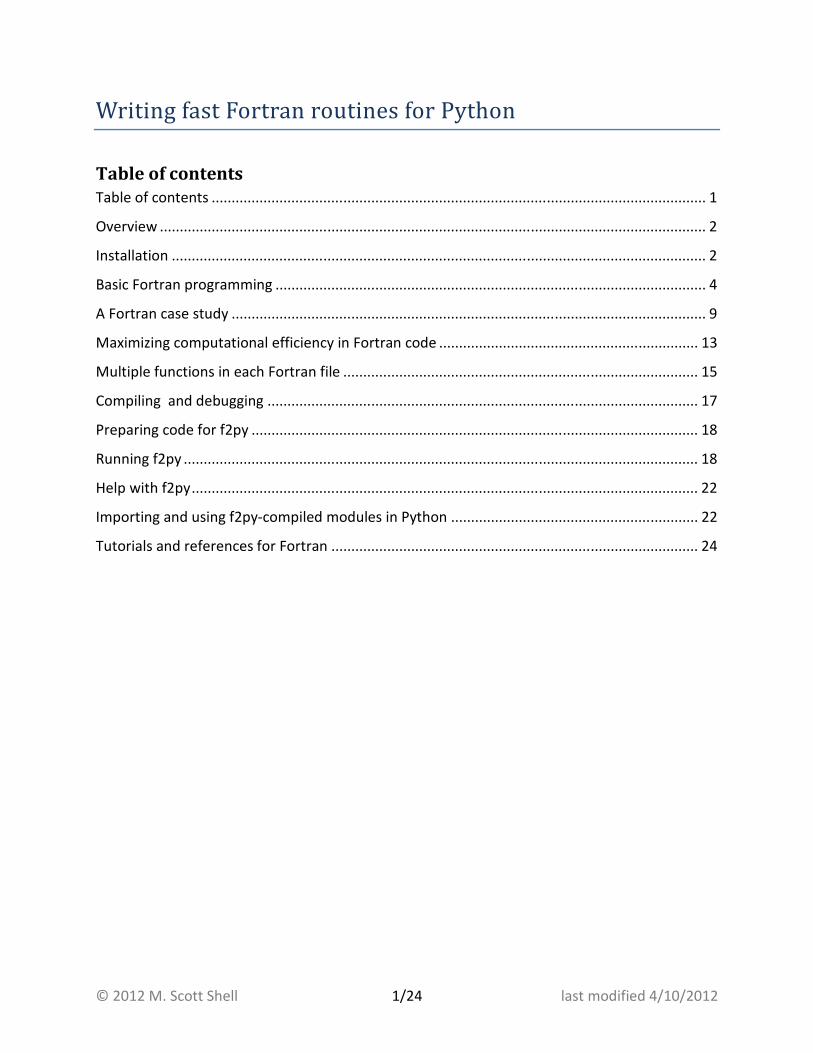
First, click on the variable Path and hit Edit. Then you want to add two items to the end of the

list in “variable value”. Add the text “;c:\python27;c:\python27\scripts”. Make sure there is a

semicolon but no spaces in between this text and whatever preceded it. (Note: whatever

currently exists in “Path” for your machine may differ from the image below. Be sure to keep

the existing text.)

Click ok and then go back to the “Environment Variables” window. Click on New in the “System

Variables” section. You will add a new variable “C_INCLUDE_PATH” with value

“c:\gfortran\include”:

Basic Fortran programming

Before we begin compiling routines, we need some background on programming in Fortran.

Fortunately, we only need to know the basics of the Fortran language since we will only be

writing numerical functions and not coding entire Fortran projects.

We will be using the Fortran 90 standard. There are older versions of Fortran, notably Fortran

77, that are much more difficult to read and use. Fortran 90 files all end in the extension .f90

and we can put multiple functions in a single .f90 file—these functions will eventually each

appear as separate member functions of the Python module we make from this Fortran file.

Fortran 90 code is actually fairly straightforward to develop, but it is important to keep in mind

some main differences from Python:

• Fortran is not case-sensitive. That is, the names atom, Atom, and ATOM all

designate the same variable.


• The comment character is an explanation point, “!”, instead of the pound sign in Python.

• Spacing is unimportant in Fortran. Instead of using spacing to show the commands

included with a subroutine or loop, Fortran uses beginning and closing statements. For

example, subroutines begin with subroutine MyFunction(….) and end with

end subroutine .

• Fortran does make a distinction between functions that return single variable values and

subroutines that do not return anything but that can modify the contents of variables

sent to it. However, in writing code to be compiled for Python, we will always write

subroutines and therefore will not need to worry about functions. We will often use the

nomenclature "function" interchangeably with subroutine.

• Fortran does not have name binding. Instead, if you change the value of a variable

passed to a subroutine via the assignment operation (=), the value of that variable is

changed for good. Fortunately, Fortran lets us declare whether or not variables can be

modified in functions, and a compile error will be thrown if we violate our own rules.

• Every variable should be typed. That means that, at the beginning of a function, we

should specify the type and size of every variable passed to it, passed from it, and

created during it. This is very important to the speed of routines. More on this later.

• Fortran has no list, dictionary, or tuple capabilities. It only has arrays. When we iterate

over an array using a loop, we must always create an integer variable that is the loop

index. Moreover, Fortran loops are inclusive of the upper bound.

• Fortran uses parenthesis () rather than brackets [] to access array elements.

• Fortran array indices start at 1 by default, rather than at 0 as in Python. This can be very

confusing, and we will always explicitly override this behavior so that arrays start at 0.

Let’s start with a specific example to get us going. We will write a function that takes in a (N,3)

array of N atom positions, computes the centroid (the average position), and makes this point

the origin by centering the original array. In Python / NumPy, we could accomplish this task

using a single line:

Pos = Pos – Pos.mean(axis=0)

An equivalent Fortran subroutine would look the following:

subroutine CenterPos(Pos, Dim, NAtom) implicit none integer, intent(in) :: Dim, NAtom


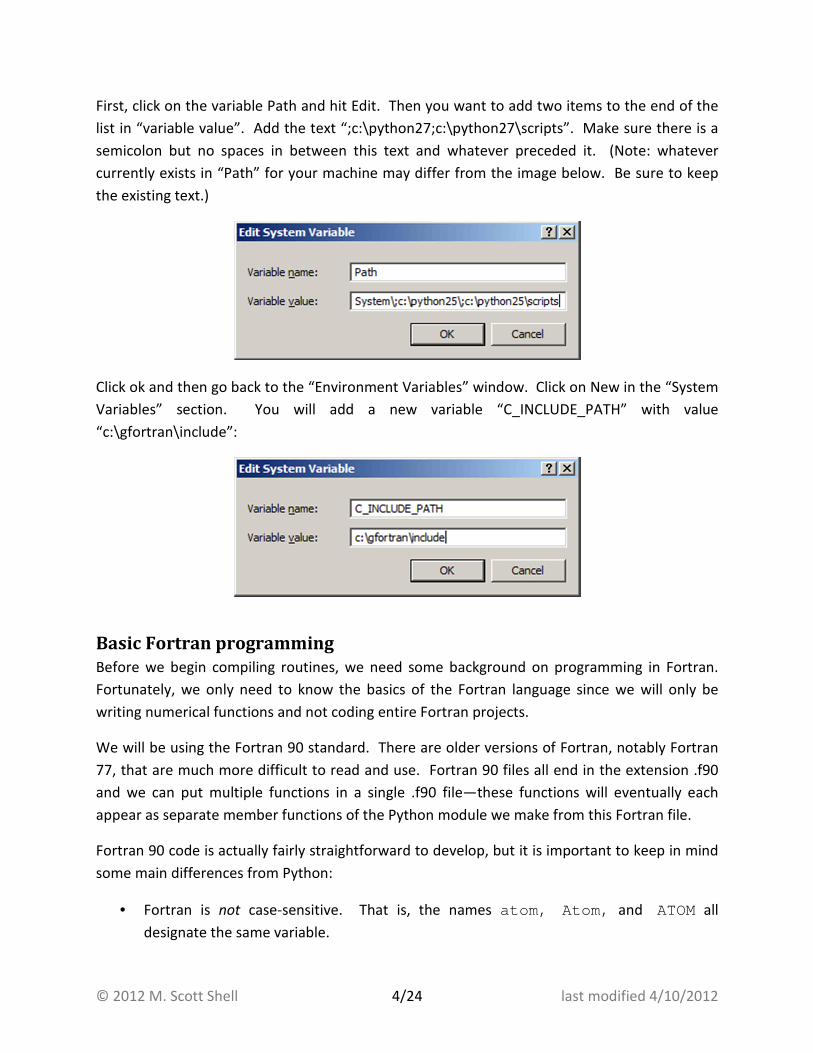
real(8), intent(inout), dimension(0:NAtom-1, 0: Dim-1) :: Pos real(8), dimension(0:Dim-1) :: PosAvg integer :: i, j PosAvg = sum(Pos, 1) / dble(NAtom) do i = 0, NAtom - 1 do j = 0, Dim - 1 Pos(i,j) = Pos(i,j) - PosAvg(j) end do end do end subroutine

In the above example, we defined a subroutine called CenterPos that takes three arguments:

the array Pos , the dimensionality Dim, and the number of atoms NAtom. The subroutine is

entirely contained within the initial subroutine and end subroutine statements.

Immediately after the declaration statement, we use the phrase implicit none . It is a

good habit always to include this statement immediately after the declaration. It tells the

Fortran compiler to raise an error if we do not define a variable that we use. Defining variables

is critical to the speed of our code.

Next we have a series of statements that define all variables, including those that are sent to

the function. These statements have the following forms. For arguments to our function that

are single values, we use:

type TYPE, intent( INTENT) :: NAME

For array arguments, we use:

type TYPE, intent( INTENT), dimension( DIMENSIONS) :: NAME

Finally, for other variables that we use within the function, but that are not arguments/inputs

or outputs, we use:

type TYPE :: NAME

or, for arrays,

type TYPE, dimension( DIMENSIONS) :: NAME

Here, TYPE is a specifier that tells the function the numeric format of a variable. The Fortran

equivalents of Python types are:

Python / NumPy Fortran

float real(8) (also called double) int integer

bool logical


For arguments, we use the INTENT option to tell Python what we are going to do with a

variable. There are three such options,

intent meaning

in The variable is an input to the subroutine only. Its value must

not be changed during the course of the subroutine.

out The variable is an output from the subroutine only. Its input

value is irrelevant. We must assign this variable a value before

exiting the subroutine.

inout The subroutine both uses and modifies the data in the variable.

Thus, the initial value is sent and we ultimately make

modifications base on it.

For array arguments, we also specify the DIMENSIONS of the arrays. For multiple dimensions,

we use comma-separated lists. The colon “:” character indicates the range of the dimension.

Unlike Python, however, the upper bound is inclusive. The statement

real(8), intent(inout), dimension(0:NAtom-1, 0:Dim- 1) :: Pos

says that the first axis of Pos varies from 0 to and including NAtom-1 , and the second axis

from 0 to and including Dim-1 . We could have also written this statement as

real(8), intent(inout), dimension(NAtom, Dim) :: Po s

In which case the lower bound of each dimension would have been 1 rather than 0. Instead,

we explicitly override this behavior to keep Fortran array indexing the same as that in Python,

for clarity in our programming.

Notice that the dimensions are variables that we must declare in and pass to the subroutine

when it is called. This, again, is a step that helps achieve faster code. Eventually f2py will

automatically pass these dimensions when the Fortran code is called as a Python module, so

that these dimensional arguments are hidden. For that reason, one should always put any

arguments that specify dimensions at the end of the argument list. Notice that all of the

dimension variables are at the end of our subroutine declaration:

subroutine CenterPos(Pos, Dim, NAtom)

Notice that we can list multiple variable names that have the same type, dimensions (if array),

and intent (if arguments) on the same line in place of NAME.

In addition to the subroutine arguments, we define three additional variables that are used only

within our function, created upon entry and destroyed upon exit:

real(8), dimension(0:Dim-1) :: PosAvg


integer :: i, j

PosAvg is a length-three array that we will use to hold the centroid position we compute. The

integers i and j are the indices we will use when writing loops.

The first line of our program computes the centroid (average position) of our array:

PosAvg = sum(Pos, 1) / dble(NAtom)

The Fortran function sum takes an array argument and sums it, optionally over a specified

dimension. Here, we indicate a summation over the first axis, that corresponding to the

particle number. In other words, Fortran sums all of the x, y, and z values separately and

returns a length-three array. It is very important to notice here that the first axis of an array is

indicated with 1 rather than 0, as would be the case in Python. This is because Fortran ordering

naturally begins at 1.

The dble function above takes the integer NAtom and converts it to a double-precision

number, e.g., of type real(8). It is a good idea to explicitly convert types using such

functions in Fortran. Not doing so will force the compiler to insert conversions that many not

be what we desired, and could result in extra unanticipated steps that might slow performance.

In addition to dble , int(X) will convert any argument X to an integer type.

The lines that follow modify the Pos array to subtract the centroid positions from it:

do i = 0, NAtom - 1 do j = 0, Dim - 1 Pos(i,j) = Pos(i,j) - PosAvg(j) end do end do

Notice that we have two loops that iterate over the array indices. Each loop has the following

form:

do VAR = START, STOP COMMANDS end do

In Fortran, such do loops involve integers and are inclusive of both the starting and stopping

values. Indentation here is optional and just for ease of reading, as it is the end do command

that signals the end of a loop.

Like Python, Fortran allows array operations. What this means internally is that Fortran will

write out the implied do loop over array elements if we perform array calculations. We could

therefore simplify the above code by removing the inner loop:


subroutine CenterPos(Pos, Dim, NAtom) implicit none integer, intent(in) :: Dim, NAtom real(8), intent(inout), dimension(0:NAtom-1, 0: Dim-1) :: Pos real(8), dimension(0:Dim-1) :: PosAvg integer :: i PosAvg = sum(Pos, 1) / dble(NAtom) do i = 0, NAtom - 1 Pos(i,:) = Pos(i,:) - PosAvg(:) end do end subroutine

Here, we use Fortran slicing notation to indicate that we want to apply the mathematical

operation to each array element.

Slicing of Fortran arrays is very similar to that of NumPy, and uses the start:stop:step

notation, where each of these can be optional. One small difference is that the upper bounds

of arrays are inclusive in Fortran, whereas they are exclusive in Python. In other words,

PosAvg[:2] takes elements 0 through 1 in Python and PosAvg(:2) takes elements 0

through 2 in Fortran.

There is one other, major difference between slicing arrays in Fortran and NumPy: the former

does not permit broadcasting. That means that every array in a mathematical operation

designed to operate elementwise must be the exact same dimensions and size. In NumPy, on

the other hand, broadcasting can be used to automatically up-convert arrays to higher

dimensionalities when performing such operations.

A Fortran case study

To illustrate the Fortran language, we will consider the following subroutine that computes the

total potential energy and force on each atom for a system of Lennard-Jones particles. Here,

total potential energy is given by a sum of pairwise interactions:

� =��

�� = 4� �� − �� The force in the x-direction on a particular atom is given by:

��,� = − �� = − ��


= −��

But since �� = �� − �� + �� − �� + �� − ��,

��,� = −� �� − �� ! ��

Thus, generalizing to all three coordinates and using vector notation for "�� = "� − "�: #� =� "��! ��

=� "��! $4�� % −12 �� ( + 6�� *��

=�"�� −48 �� , + 24 �� -��

These equations form the basis of our pairwise interaction loop. We notice that we will need to

compute vectors, like "��, as well as distances, like ��. In addition, a large portion of our

computational overhead will involve raising quantities to powers.

We must also consider the effects of periodic boundary conditions when computing "�� and ��.

Each particle should see only those images of other particles that are closest to it. We can

accomplish this task by finding the minimum image distance between each pair of particles "��. .

For each component, we use the rounding function nint , which returns the nearest integer

value:

"��. = "�� − /nint�"�� /⁄

Here / is the length of the simulation box, and may be a vector for non-cubic boxes. Notice that

this equation implies a separate operation for each component x, y, and z.

Finally, we have to treat the truncation of our potential. We will introduce a cutoff at a

pairwise distance �5, beyond which the value of the potential will be zero; typically �5 = 2.5� or

greater. We will also shift our entire potential up in energy by the value at �5 so that the

potential energy between any pair of particles continuously approaches zero at �5. Thus we

have:


�� = 84� �� − �� − 4� ��5�� − ��5�� ≤ �50 �� > �5

In our simulation, we will work with dimensionless units such that values for

positions/distances and energies are given in units of � and � respectively. Thus, our pairwise

potential function actually looks like:

�� = <4=�� − ��> − 4?�5�� − �5��@ �� ≤ �50 �� > �5

We are now ready to write our subroutine. A naïve implementation unoptimized for speed

might look like:

ljlib1.f90

subroutine EnergyForces(Pos, L, rc, PEnergy, Forces , Dim, NAtom) implicit none integer, intent(in) :: Dim, NAtom real(8), intent(in), dimension(0:NAtom-1, 0:Dim -1) :: Pos real(8), intent(in) :: L, rc real(8), intent(out) :: PEnergy real(8), intent(inout), dimension(0:NAtom-1, 0: Dim-1) :: Forces real(8), dimension(Dim) :: rij, Fij real(8) :: d, Shift integer :: i, j PEnergy = 0. Forces = 0. Shift = -4. * (rc**(-12) – rc**(-6)) do i = 0, NAtom - 1 do j = i + 1, NAtom - 1 rij = Pos(j,:) - Pos(i,:) rij = rij - L * dnint(rij / L) d = sqrt(sum(rij * rij)) if (d > rc) then cycle end if PEnergy = PEnergy + 4. * (d**(-12) – d* *(-6)) + Shift Fij = rij * (-48. * d**(-14) + 24. * d* *(-12)) Forces(i,:) = Forces(i,:) + Fij Forces(j,:) = Forces(j,:) - Fij enddo enddo end subroutine

Let’s consider the features of this subroutine. The arguments Pos , L, and rc are all sent to the

function using the intent(in) attribute and are not modified. The float PEnergy is

intent(out) , meaning that it will be returned from our function. The array Forces is

intent(inout) . The reason that we did not use intent(out) for Forces is that this

will ultimately imply creation of a new array each time the function is called, after we compile


with f2py. By declaring the array as intent(inout) , we will be able to re-use an existing

array for storing the forces, thus avoiding any performance hit that would accompany new

array creation. Finally, the arguments Dim and NAtom give the sizes of various array

dimensions.

Upon entering the subroutine, we zero the values of the potential energy and forces since we

will add to these variables during the pairwise loop. We also precalculate the values of any

constants that will be used during the loop, such as the energy shift due to the pairwise

potential truncation.

In the pairwise loop, we compute the minimum image distance using the code

rij = Pos(j,:) - Pos(i,:) rij = rij - L * dnint(rij / L)

Notice that rij is a length-three array and thus these lines are actually implied loops over each

element. Here, dnint is the Fortran function returning the nearest integer of its argument as

a type double or real(8) (the same as a Python float).

The absolute distance is computed and we then determine whether or not a pair of atoms is

beyond the distance cutoff:

d = sqrt(sum(rij * rij)) if (d > rc) then cycle end if

The cycle statement in Fortran is equivalent to continue in Python, and it immediately

causes the innermost loop to advance and return to the next iteration. Here, we use it to skip

ahead to the next atom pair if two atoms are beyond the cutoff.

Notice the formatting of the if statement. In general, Fortran conditional statements have the

form:

if ( CONDITION) then COMMANDS else if ( CONDITION) then COMMANDS else COMMANDS end if

The test condition can be any conditional expression built from comparison operators,

parenthesis, and compound statements. In Fortran, conditional comparisons are given by ==, <,

>, <=, >= and /=. Only the last of these, which signifies “not equals to”, is different from

Python. Moreover, in Fortran compound expressions can be written using .and. , .or. , and


.not. which differ from Python only by the presence of a preceding and trailing period.

Similarly, the Boolean constants in Fortran are written as .true. and .false.

After calculating the force, we add this vector to the force array for particle i and the negative

vector for particle j in the loop:

Fij = rij * (-48. * d**(-14) + 24. * d**(-12)) Forces(i,:) = Forces(i,:) + Fij Forces(j,:) = Forces(j,:) – Fij

Notice that, like Python, the power operator is written as ** .

In addition to the sqrt function used in this example, Fortran provides a large number of

mathematical operations, almost all of which can be used to operate on entire arrays at a time.

These functions include:

mod, sin, cos, tan, cotan, asin, acos, atan, sinh, cosh, tanh, asinh, acosh, atanh, exp, log, log10, sqrt, ceiling, floor, nint, erf, erfc, huge, tiny, epsilon

For many of these, the default versions of the functions return single-precision numbers. To

obtain double-precision return values, the equivalent of Python floats, there are versions of the

functions that start with “d”, such as dnint from nint .

In addition there are a number of functions that return information about arrays or perform

array-specific mathematical operations:

count, sum, product, minval, maxval, minloc, maxloc , matmul, transpose

Many of these functions accept an optional argument axis=X that will perform the indicated

operation over the specified axis only, returning an array of one smaller dimension. Keep in

mind that in Fortran the first axis is axis=1 , as opposed to Python’s axis=0 .

Maximizing computational efficiency in Fortran code

While the above code appears simple and straightforward, there are a number of ways in which

it might be rewritten to require much fewer floating point calculations.

First, we never need to find the absolute distance between two particles; rather, all

computations can be rewritten in terms of the squared distance. Thus we can remove the

square root operation, which will result in significant time savings.


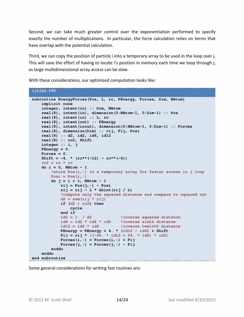
Second, we can take much greater control over the exponentiation performed to specify

exactly the number of multiplications. In particular, the force calculation relies on terms that

have overlap with the potential calculation.

Third, we can copy the position of particle i into a temporary array to be used in the loop over j.

This will save the effort of having to locate i’s position in memory each time we loop through j,

as large multidimensional array access can be slow.

With these considerations, our optimized computation looks like:

ljlib2.f90

subroutine EnergyForces(Pos, L, rc, PEnergy, Forces , Dim, NAtom) implicit none integer, intent(in) :: Dim, NAtom real(8), intent(in), dimension(0:NAtom-1, 0:Dim -1) :: Pos real(8), intent(in) :: L, rc real(8), intent(out) :: PEnergy real(8), intent(inout), dimension(0:NAtom-1, 0: Dim-1) :: Forces real(8), dimension(Dim) :: rij, Fij, Posi real(8) :: d2, id2, id6, id12 real(8) :: rc2, Shift integer :: i, j PEnergy = 0. Forces = 0. Shift = -4. * (rc**(-12) – rc**(-6)) rc2 = rc * rc do i = 0, NAtom – 1 !store Pos(i,:) in a temporary array for faster acc ess in j loop Posi = Pos(i,:) do j = i + 1, NAtom - 1 rij = Pos(j,:) - Posi rij = rij - L * dnint(rij / L) !compute only the squared distance and compare to s quared cut d2 = sum(rij * rij) if ( d2 > rc2 ) then cycle end if id2 = 1. / d2 !inverse squared distance id6 = id2 * id2 * id2 !inverse sixth distance id12 = id6 * id6 !inverse twelv th distance PEnergy = PEnergy + 4. * ( id12 – id6 ) + Shift Fij = rij * ((-48. * id12 + 24. * id6) * id2) Forces(i,:) = Forces(i,:) + Fij Forces(j,:) = Forces(j,:) - Fij enddo enddo end subroutine

Some general considerations for writing fast routines are:


• Store values that are used multiple times in temporary variables to avoid repeating

calculations. In the above example, �� was used a number of times for each pair and

stored as its own variable id6 .

• Break down large polynomial expressions so that fewer multiplications are needed. For

example, x**3+x**2+x+1 requires four multiplication and three addition operations.

Alternatively, x*(x*(x+1)+1)+1 requires only two multiplication and three addition

operations, but gives the same result. In a similar manner, x**8 can be evaluated

fastest by ((x**2)**2)**2 .

• If expensive mathematical operations like log, exp, or sqrt can be avoided, rewrite your

code to do so.

• If the same elements of a large array are to be accessed many times in succession during

a loop, copy these values into a temporary variable first. Fortran will be able to read

and write values in variables or smaller, single-dimensional arrays much faster than in

large arrays because memory access can be slow and small variables can be optimized

to sit in faster parts of memory.

• In Fortran, arrays are traversed most efficiently in memory if the leftmost array index

varies the fastest. For example, a double loop over Pos(i,j) is the fastest if i is the

inner loop and j the outer. Similarly, expressions like Pos(:,j) are faster than

Pos(j,:) . Unfortunately, writing code in this way is not always possible given the way

in which it is natural to define arrays in Python and how Python passes variables to

Fortran. In the above example, we were not able to make the inner index vary fastest

because Pos was passed with the (x,y,z) coordinates in the second index, which we

need to access all at one time. However, if given the option, choose loops that vary the

fastest over the leftmost array indices.

Multiple functions in each Fortran file

We can put multiple subroutines inside the same Fortran file. Generally it is a good idea to

group functions together in files by their purpose and level of generality. In other words, keep

functions specific to the potential energy function in a separate Fortran file from those which

perform generic geometric manipulations (e.g., rotation of a rigid body). When compiled for

Python, all of the subroutines in a given Fortran file will appear as functions in the same

imported module.

Here is the example from above extended with a subroutine that advances the positions and

velocities of each atom using the velocity Verlet algorithm:


ljlib3.f90

subroutine EnergyForces(Pos, L, rc, PEnergy, Forces , Dim, NAtom) implicit none integer, intent(in) :: Dim, NAtom real(8), intent(in), dimension(0:NAtom-1, 0:Dim -1) :: Pos real(8), intent(in) :: L, rc real(8), intent(out) :: PEnergy real(8), intent(inout), dimension(0:NAtom-1, 0: Dim-1) :: Forces real(8), dimension(Dim) :: rij, Fij, Posi real(8) :: d2, id2, id6, id12 real(8) :: rc2, Shift integer :: i, j PEnergy = 0. Forces = 0. Shift = -4. * (rc**(-12) – rc**(-6)) rc2 = rc * rc do i = 0, NAtom – 1 !store Pos(i,:) in a temporary array for fa ster access in j loop Posi = Pos(i,:) do j = i + 1, NAtom - 1 rij = Pos(j,:) - Posi rij = rij - L * dnint(rij / L) !compute only the squared distance and compare to squared cut d2 = sum(rij * rij) if (d2 > rc2) then cycle end if id2 = 1. / d2 !inverse squar ed distance id6 = id2 * id2 * id2 !inverse sixth distance id12 = id6 * id6 !inverse twelv th distance PEnergy = PEnergy + 4. * (id12 – id6) + Shift Fij = rij * ((-48. * id12 + 24. * id6) * id2) Forces(i,:) = Forces(i,:) + Fij Forces(j,:) = Forces(j,:) - Fij enddo enddo end subroutine subroutine VVIntegrate(Pos, Vel, Accel, L, CutSq, d t, KEnergy, PEnergy, Dim, NAtom) implicit none integer, intent(in) :: Dim, NAtom real(8), intent(in) :: L, CutSq, dt real(8), intent(inout), dimension(0:NAtom-1, 0: Dim-1) :: Pos, Vel, Accel real(8), intent(out) :: KEnergy, PEnergy external :: EnergyForces Pos = Pos + dt * Vel + 0.5 * dt*dt * Accel Vel = Vel + 0.5 * dt * Accel call EnergyForces(Pos, L, CutSq, PEnergy, Accel , Dim, NAtom) Vel = Vel + 0.5 * dt * Accel KEnergy = 0.5 * sum(Vel*Vel) end subroutine

Notice that the VVIntegrate function calls the EnergyForces function within it. When a

Fortran function calls another function, we must also declare the latter using the external

keyword as we wrote above. This tells the compiler that the function we are calling lies

somewhere else in the code we wrote. In addition, called subroutines must be preceded with

the keyword call .


Compiling and debugging

Once we have written our Fortran source code, we must compile it. Ultimately this will be done

automatically by f2py in the creation of a Python module from the .f90 file. However, to debug

our code, it is often useful to first try to compile the Fortran source directly. To compile our

code above, we write at the command line:

c:\> gfortran -c ljlib3.f90

If there were no errors in our program, gfortran will return quietly with no output and a file

ljlib3.o will have been created, an object file that can be subsequently linked into an executable

file. We will have no use for the .o file here, since we are only concerned with identifying errors

in our code at this point, and thus it is safe to delete it.

If gfortran finds a problem with our code, it will return an error message. For example, if we

used the assignment k=1 in our code, but forgot to explicitly define the type of k , gfortran

would return:

ljlib3.f90:50.5: k = 1 1 Error: Symbol 'k' at (1) has no IMPLICIT type

In the first line, we are given the line (50) and column (5) numbers where it found the error, as

well as the specific error message. The number 1 is used underneath the offending line to show

where the error occurred.

Sometimes our program compiles just fine, but we still experience numerical problems in

running our code. At this point, it often becomes useful to track values of variables throughout

the program execution. In Python, we could place print statements throughout the code to

periodically report on variable values. If we also need to see the values of variables during

called Fortran routines, we can similarly place print statements within our Fortran code

during test production. In Fortran a print statement has the form:

print *, var1, var2, var3

Here, one must always include the “*,” indicator after the Fortran print statement to tell it

that you want to send the values to the terminal (screen), and not to a file or attached device.

There are also many Fortran source code editors with a graphical user interface that color-code

statements and functions for ease of viewing, and that will often check for simple errors.

Professional commercial packages (e.g., not free) include the Intel Visual Fortran programming

suite:


http://www.intel.com/cd/software/products/asmo-na/eng/278834.htm

Yapakit is a free cross-platform editor, available at:

http://pagesperso-orange.fr/yapakit.fortran/

Preparing code for f2py

Generally, if we write Fortran code that strongly types and specifies intents for all variables,

then there is very little that we need to do before using f2py to convert it into a Python-

importable module. However, for array variables with the intent(inout) attribute, we

typically need to add a small directive that tells f2py how we want to deal with this particular

kind of variable. f2py directives are small comments at the beginning of lines (no preceding

spaces) that start as “!f2py ”. For intent(inout) variables, we simply add

!f2py intent(in,out) :: VAR

to the line after an argument declaration statement.

Consider the EnergyForces function. Here, we need to place an f2py directive immediately

after the type declaration for the Forces variable:

… real(8), intent(inout), dimension(0:NAtom-1, 0: Dim-1) :: Forces !f2py intent(in,out) :: Forces …

Since our directive begins with the Fortran comment character “!”, it will not affect compilation

by Fortran during debugging. However, the addition of intent(in,out) :: Forces will

tell f2py that we want the Python version of our Fortran function to treat the array Forces as

an argument and also as a return value as a part of the return tuple.

We need to similarly modify the code for VVIntegrate :

… real(8), intent(inout), dimension(0:NAtom-1, 0: Dim-1) :: Pos, Vel, Accel !f2py intent(in,out) :: Pos, Vel, Accel …

Running f2py

Once we have written and debugged our Fortran source code, we are ready to compile it into a

Python module using the f2py utility. If your environment variables are set up correctly, you

should be able to run f2py directly from the command line or terminal. Running f2py without

any arguments prints out a long help file:


c:\> f2py Usage: 1) To construct extension module sources: f2py [<options>] <fortran files> [[[only:]||[ skip:]] \ <fortran fu nctions> ] \ [: <fortran files> ...] 2) To compile fortran files and build extension mod ules: f2py -c [<options>, <build_flib options>, <ex tra options>] <fortran files> 3) To generate signature files: f2py -h <filename.pyf> ...< same options as i n (1) > Description: This program generates a Python C/API file (<modulename>module.c) that contains wrappers for given fortr an functions so that they can be called from Python. With the -c option the corresponding extension modules are built. …

f2py is a powerful utility that enables a lot of control over how modules are compiled. Here we

will only describe a specific subset of its abilities.

To compile our code into a module on a Windows platform we use a command of the following

form:

f2py –c –m MODULENAME SOURCE.f90 --fcompiler=gnu95 --compiler=mingw32

Here, MODULENAME is the name we want for our module after it is compiled. SOURCE.f90 is

the name of the file containing the Fortran source code. The –c and –m flags indicate

compilation and the name specification, respectively. The option --fcompiler=gnu95 tells

f2py to use the GFortran compiler that we downloaded and installed earlier. There are other

Fortran compilers that will work with f2py that could be specified here. To see what compilers

are present and recognized on your system, use the following command:

c:\> f2py –c --help-fcompiler Fortran compilers found: --fcompiler=compaqv DIGITAL or Compaq Visual For tran Compiler (6.6) --fcompiler=gnu95 GNU Fortran 95 compiler (4.4 .0) Compilers available for this platform, but not foun d: --fcompiler=absoft Absoft Corp Fortran Compiler --fcompiler=g95 G95 Fortran Compiler --fcompiler=gnu GNU Fortran 77 compiler --fcompiler=intelev Intel Visual Fortran Compile r for Itanium apps --fcompiler=intelv Intel Visual Fortran Compile r for 32-bit apps Compilers not available on this platform: --fcompiler=compaq Compaq Fortran Compiler --fcompiler=hpux HP Fortran 90 Compiler --fcompiler=ibm IBM XL Fortran Compiler --fcompiler=intel Intel Fortran Compiler for 3 2-bit apps --fcompiler=intele Intel Fortran Compiler for I tanium apps --fcompiler=intelem Intel Fortran Compiler for E M64T-based apps


--fcompiler=lahey Lahey/Fujitsu Fortran 95 Com piler --fcompiler=mips MIPSpro Fortran Compiler --fcompiler=nag NAGWare Fortran 95 Compiler --fcompiler=none Fake Fortran compiler --fcompiler=pg Portland Group Fortran Compi ler --fcompiler=sun Sun or Forte Fortran 95 Comp iler --fcompiler=vast Pacific-Sierra Research Fort ran 90 Compiler For compiler details, run 'config_fc --verbose' set up command.

Part of the f2py process involves the automated writing and compilation of C wrapper code

around the Fortran routines. The option --compiler=mingw32 tells f2py to use the

MinGW C compiler that comes with gfortran. This compiler is specific to the Windows system.

On other systems, this option might be omitted to use the default C compiler, or another C

compiler could be specified directly (e.g., --compiler=gcc ).

Running f2py for our Lennard-Jones example looks something like the following:

c:\>f2py -c -m ljlib ljlib3.f90 --fcompiler=gnu95 - -compiler=mingw32 Ignoring "Python was built with Visual Studio versi on 7.1, and extensions need to be built with the same version of the compiler, but it isn' t installed." (one should fix me in fco mpiler/compaq.py) running build running config_cc unifing config_cc, config, build_clib, build_ext, b uild commands --compiler options running config_fc unifing config_fc, config, build_clib, build_ext, b uild commands --fcompiler options running build_src building extension "ljlib" sources f2py options: [] f2py:> c:\docume~1\shell\locals~1\temp\tmpl4tj-f\sr c.win32-2.5\ljlibmodule.c creating c:\docume~1\shell\locals~1\temp\tmpl4tj-f creating c:\docume~1\shell\locals~1\temp\tmpl4tj-f\ src.win32-2.5 Reading fortran codes... Reading file 'ljlib3.f90' (format:free) Post-processing... Block: ljlib Block: energyforces Block: vvintegrate Post-processing (stage 2)... Building modules... Building module "ljlib"... Constructing wrapper function "ener gyforces"... penergy,forces = energyforces(pos ,l,rc,forces,[dim,natom]) Constructing wrapper function "vvin tegrate"... pos,vel,accel,kenergy,penergy = v vintegrate(pos,vel,accel,l,cutsq,dt,[di m,natom]) Wrote C/API module "ljlib" to file "c:\docu me~1\shell\locals~1\temp\tmpl4tj-f\src.win 32-2.5/ljlibmodule.c" adding 'c:\docume~1\shell\locals~1\temp\tmpl4tj-f \src.win32-2.5\fortranobject.c' to sour ces. adding 'c:\docume~1\shell\locals~1\temp\tmpl4tj-f \src.win32-2.5' to include_dirs. copying C:\Python25\lib\site-packages\numpy\f2py\sr c\fortranobject.c -> c:\docume~1\shell\ locals~1\temp\tmpl4tj-f\src.win32-2.5 copying C:\Python25\lib\site-packages\numpy\f2py\sr c\fortranobject.h -> c:\docume~1\shell\ locals~1\temp\tmpl4tj-f\src.win32-2.5 running build_ext customize Mingw32CCompiler customize Mingw32CCompiler using build_ext customize Gnu95FCompiler Found executable C:\gfortran\bin\gfortran.exe Found executable C:\gfortran\bin\gfortran.exe customize Gnu95FCompiler using build_ext building 'ljlib' extension compiling C sources


C compiler: gcc -mno-cygwin -O2 -Wall -Wstrict-prot otypes creating c:\docume~1\shell\locals~1\temp\tmpl4tj-f\ Release creating c:\docume~1\shell\locals~1\temp\tmpl4tj-f\ Release\docume~1 creating c:\docume~1\shell\locals~1\temp\tmpl4tj-f\ Release\docume~1\shell creating c:\docume~1\shell\locals~1\temp\tmpl4tj-f\ Release\docume~1\shell\locals~1 creating c:\docume~1\shell\locals~1\temp\tmpl4tj-f\ Release\docume~1\shell\locals~1\temp creating c:\docume~1\shell\locals~1\temp\tmpl4tj-f\ Release\docume~1\shell\locals~1\temp\tm pl4tj-f creating c:\docume~1\shell\locals~1\temp\tmpl4tj-f\ Release\docume~1\shell\locals~1\temp\tm pl4tj-f\src.win32-2.5 compile options: '-Ic:\docume~1\shell\locals~1\temp \tmpl4tj-f\src.win32-2.5 -IC:\Python25\ lib\site-packages\numpy\core\include -IC:\Python25\ include -IC:\Python25\PC -c' gcc -mno-cygwin -O2 -Wall -Wstrict-prototypes -Ic:\ docume~1\shell\locals~1\temp\tmpl4tj-f\ src.win32-2.5 -IC:\Python25\lib\site-packages\numpy \core\include -IC:\Python25\include -IC :\Python25\PC -c c:\docume~1\shell\locals~1\temp\tm pl4tj-f\src.win32-2.5\fortranobject.c - o c:\docume~1\shell\locals~1\temp\tmpl4tj-f\Release \docume~1\shell\locals~1\temp\tmpl4tj-f \src.win32-2.5\fortranobject.o Found executable C:\gfortran\bin\gcc.exe gcc -mno-cygwin -O2 -Wall -Wstrict-prototypes -Ic:\ docume~1\shell\locals~1\temp\tmpl4tj-f\ src.win32-2.5 -IC:\Python25\lib\site-packages\numpy \core\include -IC:\Python25\include -IC :\Python25\PC -c c:\docume~1\shell\locals~1\temp\tm pl4tj-f\src.win32-2.5\ljlibmodule.c -o c:\ docume~1\shell\locals~1\temp\tmpl4tj-f\Release\docu me~1\shell\locals~1\temp\tmpl4tj-f\src. win32-2.5\ljlibmodule.o compiling Fortran sources Fortran f77 compiler: C:\gfortran\bin\gfortran.exe -Wall -ffixed-form -fno-second-undersco re -mno-cygwin -O3 -funroll-loops -march=nocona -mm mx -msse2 -fomit-frame-pointer -malign- double Fortran f90 compiler: C:\gfortran\bin\gfortran.exe -Wall -fno-second-underscore -mno-cygwi n -O3 -funroll-loops -march=nocona -mmmx -msse2 -fo mit-frame-pointer -malign-double Fortran fix compiler: C:\gfortran\bin\gfortran.exe -Wall -ffixed-form -fno-second-undersco re -mno-cygwin -Wall -fno-second-underscore -mno-cy gwin -O3 -funroll-loops -march=nocona - mmmx -msse2 -fomit-frame-pointer -malign-double compile options: '-Ic:\docume~1\shell\locals~1\temp \tmpl4tj-f\src.win32-2.5 -IC:\Python25\ lib\site-packages\numpy\core\include -IC:\Python25\ include -IC:\Python25\PC -c' gfortran.exe:f90: ljlib3.f90 C:\gfortran\bin\gfortran.exe -Wall -mno-cygwin -Wal l -mno-cygwin -shared c:\docume~1\shell \locals~1\temp\tmpl4tj-f\Release\docume~1\shell\loc als~1\temp\tmpl4tj-f\src.win32-2.5\ljlibmo dule.o c:\docume~1\shell\locals~1\temp\tmpl4tj-f\Re lease\docume~1\shell\locals~1\temp\tmpl 4tj-f\src.win32-2.5\fortranobject.o c:\docume~1\she ll\locals~1\temp\tmpl4tj-f\Release\mdli b.o -Lc:\gfortran\lib\gcc\i586-pc-mingw32\4.4.0 -LC :\Python25\libs -LC:\Python25\PCbuild - lpython25 -lgfortran -o .\ljlib.pyd running scons Removing build directory c:\docume~1\shell\locals~1 \temp\tmpl4tj-f

A fair amount of text is outputted when running f2py. You will know that your code has

compiled successfully when (1) the final lines of the f2py output contain “Removing build

directory…” and there are no signs of errors, and (2) a compiled module file now exists. On

Windows, your module file will end in .pyd, while on Linux it will typically end in .so. The name

of your file is that which you specified in the MODULENAME option.

The f2py utility will generate automatically all of the code necessary to pass NumPy arrays in

between Python and your compiled Fortran routines. In particular, it makes sure that function

arguments obey the right types and dimensioning. As a part of this effort to make sure Python

arrays are Fortran-friendly, NumPy can sometimes make a copy of an input array to send to the

compiled function.

Sometimes it is convenient to know when copies are made of arrays sent to Fortran routines,

rather than the original Python arrays themselves, since such copying can create a performance


hit. One can compile f2py with the additional option -DF2PY_REPORT_ON_ARRAY_COPY=1 to

have Fortran-compiled routines print out messages in real-time each time such a copying event

occurs. This is useful for debugging / optimizing code, but final production code should not use

this option.

Help with f2py

There are a number of online resources for reading about additional options with and for

troubleshooting the f2py utility. The main website can be found at the SciPy development

page:

http://www.scipy.org/F2py

More extensive documentation can be found at links therein, and at the following:

http://cens.ioc.ee/projects/f2py2e/

For those who are using f2py on Windows,

http://www.scipy.org/F2PY_Windows

Importing and using f2py-compiled modules in Python

Once we have compiled our Fortran source code into a module using f2py, it is as easy to

import as any other module:

>>> import ljlib

f2py embeds information about the functions it compiles into docstrings. To see these

docstrings, use the print statement with the __doc__ special property:

>>> print ljlib.__doc__ This module 'ljlib' is auto-generated with f2py (ve rsion:2_5972). Functions: penergy,forces = energyforces(pos,l,rc,forces,dim =shape(pos,1),natom= shape(pos,0)) pos,vel,accel,kenergy,penergy = vvintegrate(pos,v el,accel,l,cutsq,dt,dim= shape(pos,1),natom=shape(pos,0))

Here, the docstring tells us that the module contains two functions, energyforces and

vvintegrate . Notice that f2py converts all Fortran variable and function names to

lowercase format by default.


In addition to their names, the module docstring tells us the format of a call to each of the

functions. We can get more detailed information by examining the docstrings of the individual

functions:

>>> print ljlib.energyforces.__doc__ energyforces - Function signature: penergy,forces = energyforces(pos,l,rc,forces,[di m,natom]) Required arguments: pos : input rank-2 array('d') with bounds (natom, dim) l : input float rc : input float forces : rank-2 array('d') with bounds (natom,di m) Optional arguments: dim := shape(pos,1) input int natom := shape(pos,0) input int Return objects: penergy : float forces : rank-2 array('d') with bounds (natom,dim )

Here, we are told that there are four arguments we must provide: pos , l , rc , and forces .

These arguments correspond to any for which we specified the intent(in) or

intent(inout) attributes. However, we do not need to specify the dimension variables

dim and natom , as these will be taken automatically from the shape of the argument pos .

The docstring also tells us that the function will return two arguments, penergy and forces .

These correspond to any Fortran arguments for which we specified intent(out) or

intent(inout) . Thus a call from Python to the energyforces routine would look like:

>>> penergy, forces = ljlib.energyforces(pos, l, rc , forces)

where we would have needed to supply the vector of positions, box length, cutoff, and force

array. If we had specified intent(out) for forces , it would not have appeared as an

argument and Python instead would have created a new force array with each function call.

Similarly, we can examine the docstring of the vvintegrate function:

>>> print ljlib.vvintegrate.__doc__ vvintegrate - Function signature: pos,vel,accel,kenergy,penergy = vvintegrate(pos,v el,accel,l,cutsq,dt, [dim,natom]) Required arguments: pos : rank-2 array('d') with bounds (natom,dim) vel : rank-2 array('d') with bounds (natom,dim) accel : rank-2 array('d') with bounds (natom,dim ) l : input float cutsq : input float dt : input float Optional arguments: dim := shape(pos,1) input int natom := shape(pos,0) input int


Return objects: pos : rank-2 array('d') with bounds (natom,dim) vel : rank-2 array('d') with bounds (natom,dim) accel : rank-2 array('d') with bounds (natom,dim) kenergy : float penergy : float

A call to vvintegrate would therefore look like:

>>> pos, vel, accel, kenergy, penergy = ljlib.vvint egrate(pos, vel, accel, ... l, cutsq, dt)

Note that f2py automatically makes the conversions / equivalencies of Fortran real(8) and

Python float types.

And that’s it! You are now ready to use your Fortran routines with Python.

Tutorials and references for Fortran

It is beyond the scope of this document to cover the entire Fortran language. However, a

number of excellent tutorials for Fortran programming are available online. Keep in mind that

many of these discuss broader programmatic issues, like file input/output and modules, that

are irrelevant for the much simpler task of compiling numerical functions for Python.

http://www.dur.ac.uk/resources/its/info/guides/138fortran90.pdf

http://www.pcc.qub.ac.uk/tec/courses/f90/ohp/f90-ohp.html

http://www.cisl.ucar.edu/tcg/consweb/Fortran90/F90Tutorial/tutorial.html

http://www.cs.mtu.edu/~shene/COURSES/cs201/NOTES/fortran.html

http://wwwasdoc.web.cern.ch/wwwasdoc/f90.html

http://www.liv.ac.uk/HPC/HTMLF90Course/HTMLF90CourseSlides.html

A large reference for language constructs and available functions can be found at:

http://docs.hp.com/en/B3908-90002/

A convenient “cheat sheet” can also be found at:

http://www.pa.msu.edu/~duxbury/courses/phy480/fortran90_refcard.pdf

Documents

Writing fast Fortran routines for Python - UCSB …shell/che210d/f2py.pdfWriting fast Fortran routines for Python Table of contents Table of contents