Embed Size (px)
Citation preview

XI. OTHER TOPICS
Complicated Statistics with Nasty Properties
Bootstrap Analysis
Treat the sample as if it were the target population
Sample repeatedly without replacement to obtain many samples of the same size as the real sample
Calculate the test statistic for each sample
Examine the variation of the test statistic among bootstrapped samples to assess its dispersion.
© William D. Dupont, 2010, 2011Use of this file is restricted by a Creative Commons Attribution Non-Commercial Share Alike license.See http://creativecommons.org/about/licenses for details.

Multiple imputation of missing values
Most statistical packages, including Stata do complete case analyses. That is they discard the data on any patient who is missing any model covariate.
Multiple imputation is a method that adjusts for missing data by predicting missing values from non-missing covariates.
Lead to unbiased results if the probability of the outcome of interest is not affected by whether a specific covariate is missing.
Stata has a very comprehensive package for doing multiple imputation
Particularly useful to adjust for missing values in confounding variables.

1. Discriminatory Analysis
We often wish to place patients into two or more groups on the basis of a set of explanatory variables with a minimum of misclassification error.
We typically start of with a learning set of patients whose true classification is known. We then use these patients for developing rules to classify other patients. The three most common ways of doing this are as follows.
For example, we might wish to classify patients as
· having or not having cancer,
· benefiting or not benefiting from aggressive therapy.

· Logistic Regression
The linear predictor from a multiple logistic regression can be used to develop a classification rule. Patients whose linear predictor is greater than some value are assigned to one group; all other patients are assigned to the other.
· Classification and Regression Trees
· Neural Networks
The disadvantage is that the rule may be less than optimal if the model is mis-specified.
Þ By adjusting the cutoff point we can control the sensitivity and specificity of the rule. It is easy
to generate receiver operating characteristic curves for this method. Þ Particularly effective when used with
restricted cubic splines
Þ It can lead to a simple rule based on a weighted sum of covariates.
The advantages of this approach are

2. Classification and Regression Trees (CART)
The basic idea here is to derive a tree that consists of a series of binary decisions that lead to patient classification (Breiman et al. 1984).
Var_A < K1
Var_B < K2 Var_C < K3
Var_A < K4 Var_D < K5
TRUE
TRUE
TRUE
TRUE
TRUETRUE
FALSE
FALSE
FALSE FALSE
FALSE
Assign Patient to Group X
Assign Patient to Group Y
Assign Patient to Group X
Assign Patient to Group Y
Assign Patient to Group X
Assign Patient to Group Y

The CART graphic indicates the degree of increased homogeneity induced by each split. Trees can then be pruned back to produce a classification rule that makes clinical sense and is fairly easy to remember.
· It gives a rule that is intelligible to clinicians and can be judged by its clinical criteria.
· It often does better than logistic regression when the model for the latter is poorly specified.
The advantages of this method are
A disadvantage is that, when applied to continuous covariates it looses information due to the fact that it dichotomizes the selected variable at each split.

3. Neural Networks
This method attempts to outperforms the logistic regression approach by adopting models that varies from complex to extremely complex (Hinton 1992).
· Method usually performs only as well as the CART method or logistic regression models with
restricted cubic splines.
· Method is essentially a black box. You need a computer to
apply it and it is very difficult to gain intuitive insight into what it is doing.
Disadvantages
· Sometimes does better than logistic regression.· Great name.
Advantages

4. Meta-Analyses
This is a rather pretentious term for doing quantitative reviews of the medical literature. The English refer to these techniques as quantitative overviews, which is a far more reasonable description. However, in this country we appear to be stuck with the term meta-analysis.
The basic steps in performing a meta-analysis are as follows:
· Systematically identify all publications that may be germane to the topic of
interest.
· Use clinical judgment and statistical methods to determine whether it is reasonable to combine some or all
of the studies into a single analysis. In this case present the relative risk derived from the combined data, together with its 95% confidence interval.
· Present the results of the individual studies graphically to show the extent to which they agree or disagree.
· Review these publications. Eliminate those that are irreverent or misleading using explicitly
defined criteria.
One of the strengths of this approach is the meta-analysis
graphic.

Year ofPublication
FirstAuthor Journal
\\pmpc58\office\lectures\estronicaragua97\cardio.ppt
1971 Potocki
Hammond1979Nachtigall1979
Lafferty1985
Wilson1985Eaker1987
Croft1989Avila1990
Stampfer1991
Pol Tyg Lek
Obs GynMaturitasNEJM
Brit Med JEpidemiol
NEJM
Haymarket
Am J Obs Gyn
All Studies
0 1 2 3
Relative Risk of CVD
Prospective Studies of ERT andCardiovascular Disease
Exposure
current
past
4

· In these graphs the relative risk from each study is displayed on a single line.
· One, or preferably two, 95% confidence intervals are drawn for this combined geometric mean. These confidence intervals are usually drawn as diamonds or squares. They are calculated using either a fixed effects or random effects model.
· A vertical line depicts a weighted geometric mean of the studies. This mean is weighted by the information content of each study.
· The 95% confidence interval for each study is depicted as a horizontal line.
· The size of this square is proportional to the reciprocal of the variance of the log relative risk (often referred to as the study information).
· Each relative risk or odds ratio is plotted as a square.

a) Fixed effects model for meta-analysis
This approach assumes that all studies are measuring the same risk in a comparable way, and that the only variation between studies is due to chance.
If this assumption is false it will overestimate the precision of the combined estimate.
b) Random effects model for meta-analysis
This model assumes that that each study is estimating a different unknown relative risk that is specific to that study. These risks differ from one study to the next due to differences in study populations, study designs, or biases of one kind or another.
It assumes that these study-specific relative risks follow a log-normal distribution, and that the variation in the estimated relative risks is due both to variation in the study specific risk as well as intra-study variation of study subjects.

DerSimonian and Laird (1986) devised a way to estimate the confidence interval for the combined relative risk for this model.
It is a good idea to plot both the fixed effects and random effects confidence intervals for the combined relative risk estimate. If these intervals disagree then the inter-study variation is greater than we would expect by chance and the studies are most likely estimating different risks. In this case we need to be very cautious about combining the results of these studies.

Year ofPublication
FirstAuthor Journal
\\pmpc58\office\lectures\estronicaragua97\cardio.ppt
1971 Potocki
Hammond1979Nachtigall1979
Lafferty1985
Wilson1985Eaker1987
Croft1989Avila1990
Stampfer1991
Pol Tyg Lek
Obs GynMaturitasNEJM
Brit Med JEpidemiol
NEJM
Haymarket
Am J Obs Gyn
All Studies
0 1 2 3
Relative Risk of CVD
Prospective Studies of ERT andCardiovascular Disease
Exposure
current
past
4

DerSimonian and Laird CCT 1986
Random Effects Model for Meta-analysis
True relative risk forall women
True relative risk for
women in i th study
Relative risk estimate
from i th study BREAST:ERT:SANTIAGO 94:DERSIMONIAN

On the other hand, if these estimates agree then the studies are mutually consistent and there is no statistical reason not to combine them.

19801986198719881991
19911991
Ross 28
Brinton18
Wingo 29
Rohan 30
Dupont 31
Kaufman 32
Palmer 33
All Studies
Year First Author
0 1 2 3 4 5 6
Relative Risk of Breast Cancer
1995 Newcomb 34
1995 Stanford 35
Women with a History of Benign Breast DiseaseBreast cancer risk among ERT users compared to non-users

5. Publication bias
One of the ways that meta-analyses can be misleading is through publication bias. That is, papers may be more likely to be published if they show that a risk factor either increases or reduces some risk than if they find a relative risk near one.
When this happens it may make sense to exclude studies with a standard error of the log relative risk that is greater than some value.
In these graphs we plot the standard error of the log relative risk against log relative risk. If this plot has a funnel shape we have evidence of publication bias
Small studies are more likely to be affected by publication bias than large ones.
6. Funnel graphs
One way to check for publication bias is to plot funnel graphs (Light & Pillemer 1984).

before 1982 10 studies198219821983198319831984198419841986198619861987198719881988198919891991199119921993199419951995199519951996199619961997
ThomasHulkaVakilGambrellShermanKaufmanHorwitzHiattNomuraMcDonaldBrintonWingoHuntRohanEwertzDupontMillsKaufmanPalmerYangWeinsteinSchairerColditzStanford
SchuumanNewcomb
PerssonLeviLongneckerTavani
JNCIAm J Ob GynCa Det PrevOb GynCancerJAMAAm J MedCancerInt J CaBr Ca Res TreatBr J CaJAMABr J Ob GynMed J AustInt J CaCancerCancerAm J EpiAm J EpiCa Causes & CtlInt J EpiCa Causes & CtlNEJMJAMAAm J EpiCa Causes & CtlInt J CaEuro J Ca PrevCa Epi Biom & PrevCa Epi Biom & Prev
All Studies
0 0.5 1 1.5 2 2.5 3.0 3.5Relative Risk of Breast Cancer
First Author JournalYear ofPublication
Women Treated with ERT
\\pmpc58\of f ice\lectures\estro\nicaragua97\meta.ppt

0.0
0.1
0.2
0.3
0.4
0.5
0.4 1.0 2.0Relative Risk of Breast Cancer
Women Treated with ERT
\\pmpc58\office\lectures\estro\nicaragua97\funnel.ppt
0.6 0.8Sta
ndar
d E
rror
of L
og R
elat
ive
Ris
k
SE
SE
Permutation Tests
Cross validation Methods
False Discovery Rates
Shrinkage Analysis
Learning set Test Set Analyses
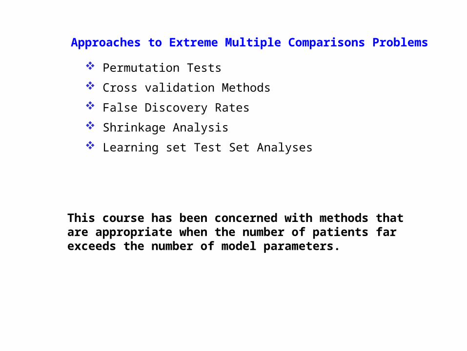
Approaches to Extreme Multiple Comparisons Problems
This course has been concerned with methods that are appropriate when the number of patients far exceeds the number of model parameters.

Diversity Among Statisticians
We all want to
Minimize probabilities of Type I errors
Minimize probabilities of Type II errors
All other things being equal, simple explanations are better than complex ones.
Science may be described as the art of systematic over-simplification — the art of discerning what we may with advantage omit.
Karl Popper
Today, reputable statisticians may disagree to some extent about the relative emphasis that should be placed on these three goals

XII. SUMMARY OF MULTIPLE REGRESSION METHODS


Table A1. Continued: continuous response, fixed effects

Table A1. Continued: continuous response, fixed effects


Table A2. Continued: dichotomous response, fixed effects

Table A2. Continued: categorical response, fixed effects

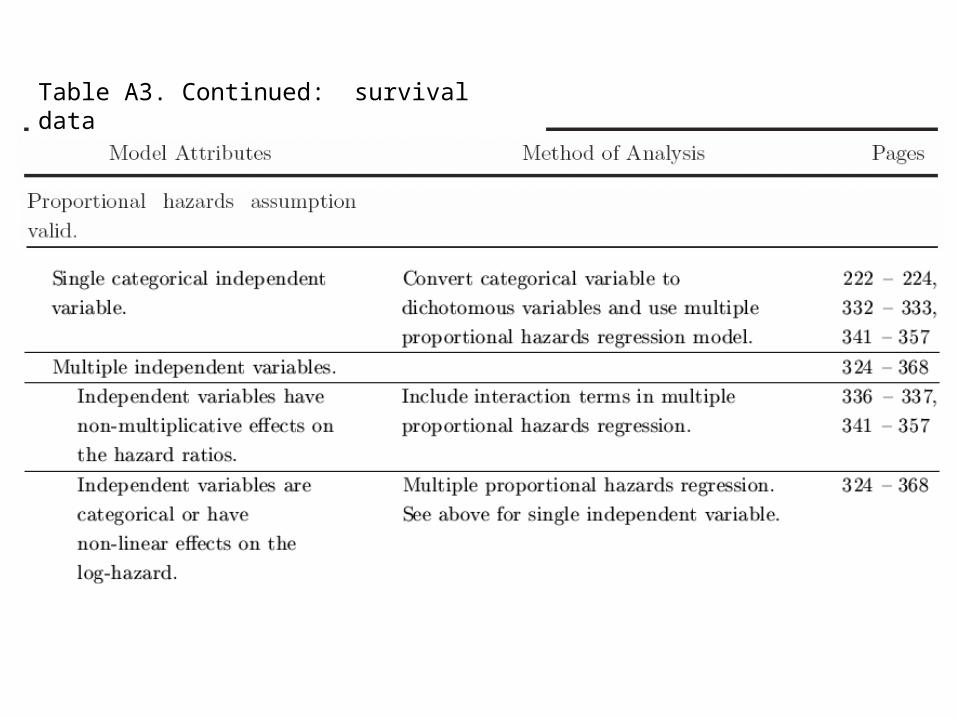
Table A3. Continued: survival data

Table A3. Continued


Problem Method
Cross-sectional StudyContinuous outcome
Normally distributed
Linear model okLinear regression
Fixed-effects analysis of variance
Non-linear modelLinear model of transformed data
Linear model with restricted cubic splines
Skewed response dataLinear model of transformed data
Dichotomous outcomeLogistic regression
Rare responsePoisson regression
Longitudinal Data
Response feature analysis
Repeated measures analysis of variance
Generalized estimating equation analysis
Problem Method
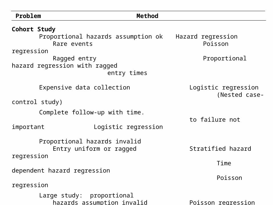
Cohort StudyProportional hazards assumption okHazard regression
Rare eventsPoisson regression
Ragged entryProportional hazard regression with ragged
entry times
Expensive data collectionLogistic regression
(Nested case-control study)
Complete follow-up with time.
to failure not important Logistic regression
Proportional hazards invalid
Entry uniform or raggedStratified hazard regression
Time dependent hazard regression
Poisson regression
Large study: proportional
hazards assumption invalid Poisson regression
Case-Control StudyUnstratified or large strata
Unconditional logistic regressionSmall strata
Conditional logistic regression

Additional Reading
A good reference for the response-compression approach to mixed-effects analysis of variance is Matthews et al. (1990).
Classic although rather mathematical references for generalized estimating equations are Liang and Zeger (1986) and Zeger and Liang (1986). Diggle et al. (2002) is an authoritative text on the analysis of longitudinal data.
Armitage and Berry (1994) discuss receiver operating characteristic curves.
Classification and regression trees are discussed by Breiman et al. (1984).
An introduction to neural networks is given by Hinton (1992). A comparison of neural nets with classification and regression trees is given by Reibnegger et al. (1991)
An introduction to meta-analysis is given by Greenland (1987). This paper also describes the fixed effects method of calculating a confidence interval for the combined relative risk estimate. The random effects method is given by DerSimonian and Laird (1986).
Harrell (2001) is an advanced text on modern regression methods.

Armitage P and Berry G: Statistical Methods in Medical Research, Third ed. Cambridge, MA: Blackwell Science, Inc., 1994.
Bernard GR, Wheeler AP, Russell JA, Schein R, Summer WR, Steinberg KP, Fulkerson WJ, Wright PE, Christman BW, Dupont WD, Higgins SB, Swindell BB: “The Effects of Ibuprofen on the Physiology and Survival of Patients with Sepsis”. New England Journal of Medicine, 1997; 336: 912-918
Breiman L, Friedman JH, Olshen RA, Stone CJ. Classification and Regression Trees. Belmont CA: Wadsworth, 1984.
Breslow NE and Day NE: Statistical Methods in Cancer Research: Vol. I The Analysis of Case-Control Studies. Lyon: IARC Scientific Publications, 1980.
Breslow NE and Day NE: Statistical Methods in Cancer Research: Vol. II. The Design and Analysis of Cohort Studies. Lyon: IARC Scientific Publications, 1987.
Cleveland WS. The Elements of Graphing Data: Monterey, CA: Wadsworth Advanced Books and Software, Bell Telephone Laboratories, Inc., 1985.
DerSimonian R. Laird N. Meta-analysis in clinical trials. Controlled Clinical Trials 1986; 7:177-188.
References
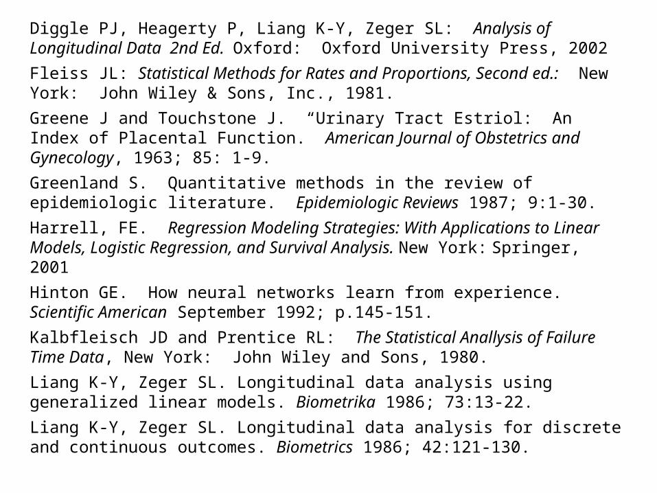
Diggle PJ, Heagerty P, Liang K-Y, Zeger SL: Analysis of Longitudinal Data 2nd Ed. Oxford: Oxford University Press, 2002
Fleiss JL: Statistical Methods for Rates and Proportions, Second ed.: New York: John Wiley & Sons, Inc., 1981.
Greene J and Touchstone J. “Urinary Tract Estriol: An Index of Placental Function. American Journal of Obstetrics and Gynecology, 1963; 85: 1-9.
Greenland S. Quantitative methods in the review of epidemiologic literature. Epidemiologic Reviews 1987; 9:1-30.
Harrell, FE. Regression Modeling Strategies: With Applications to Linear Models, Logistic Regression, and Survival Analysis. New York: Springer, 2001
Hinton GE. How neural networks learn from experience. Scientific American September 1992; p.145-151.
Kalbfleisch JD and Prentice RL: The Statistical Anallysis of Failure Time Data, New York: John Wiley and Sons, 1980.
Liang K-Y, Zeger SL. Longitudinal data analysis using generalized linear models. Biometrika 1986; 73:13-22.
Liang K-Y, Zeger SL. Longitudinal data analysis for discrete and continuous outcomes. Biometrics 1986; 42:121-130.

Light RJ, Pillemer DB. Summing Up: The Science of Reviewing Research. Cambridge, MA: Harvard University Press. 1984.
Matthews JNS, Altman DG, Campbell MJ, Royston P. Analysis of serial measurements in medical research. British Medical Journal 1990;300:230-235.
McCullagh P and Nelder JA: Generalized Linear Models, Second ed.: New York: Chapman and Hall, 1989.
McKelvey EM, Gottlieb JA, Wilson HE, Haut A, Talley RW, et al.: “Hydroxyldaunomycin (Adriamycin) Combination Chemotherapy in malignant lymphoma. Cancer, 1976; 38: 1484-1493.
Pagano M and Gauvreau K, Principles of Biostatistics, Belmont, CA: Duxbury Press, 1993.
Reibnegger G, Weiss G, Werner-Felmayer G, Judmaier G, Wachter H. Neural networks as a tool for utilizing laboratory information: Comparison with linear discriminant analysis and with classification and regression trees. Proc. Natl. Acad. Sci. USA 1991; 88:11426-11430.
Rosner B: Fundamentals of Biostatistics, Fourth ed.: Belmont, CA: Duxbury Press, 1995.

Schottenfeld D and Fraumeneni JF: Cancer Epidemiology and Prevention: Philadelphia, PA: W.B. Saunders Company, 1982.
Tuyns AJ, Pequignot G, and Jensen OM. “Le Cancer de l’oesophage en Ille-et-Villaine en fonction des niveaux de consommation d’alcool et de tabac. Bulletin du Cancer, 1977: 64: 45-60.
For additional references see
Dupont WD: Statistical Modeling for Biomedical Researchers, A Simple Introduction to the Analysis of Complex Data. 2nd Edition. Cambridge: Cambridge University Press. 2009.