Embed Size (px)
Citation preview
8/3/2019 Yaroslav D. Sergeyev- Blinking Fractals and their Quantitative Analysis Using Infinite and Infinitesimal Numbers
http://slidepdf.com/reader/full/yaroslav-d-sergeyev-blinking-fractals-and-their-quantitative-analysis-using 1/41
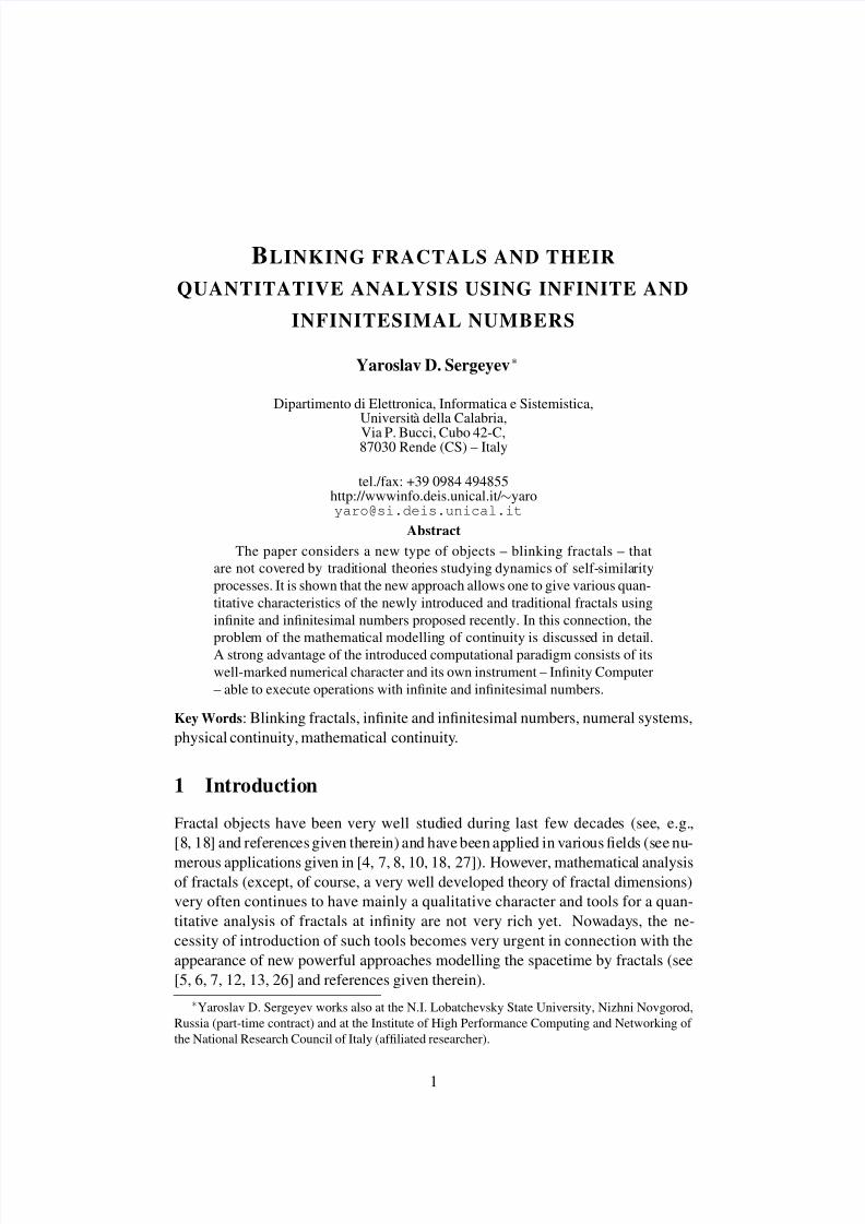
BLINKING FRACTALS AND THEIR
QUANTITATIVE ANALYSIS USING INFINITE AND
INFINITESIMAL NUMBERS
Yaroslav D. Sergeyev∗
Dipartimento di Elettronica, Informatica e Sistemistica,Universita della Calabria,
Via P. Bucci, Cubo 42-C,87030 Rende (CS) – Italy
tel./fax: +39 0984 494855http://wwwinfo.deis.unical.it/ ∼[email protected]
Abstract
The paper considers a new type of objects – blinking fractals – that
are not covered by traditional theories studying dynamics of self-similarity
processes. It is shown that the new approach allows one to give various quan-
titative characteristics of the newly introduced and traditional fractals using
infinite and infinitesimal numbers proposed recently. In this connection, the
problem of the mathematical modelling of continuity is discussed in detail.A strong advantage of the introduced computational paradigm consists of its
well-marked numerical character and its own instrument – Infinity Computer
– able to execute operations with infinite and infinitesimal numbers.
Key Words: Blinking fractals, infinite and infinitesimal numbers, numeral systems,
physical continuity, mathematical continuity.
1 Introduction
Fractal objects have been very well studied during last few decades (see, e.g.,
[8, 18] and references given therein) and have been applied in various fields (see nu-
merous applications given in [4, 7, 8, 10, 18, 27]). However, mathematical analysisof fractals (except, of course, a very well developed theory of fractal dimensions)
very often continues to have mainly a qualitative character and tools for a quan-
titative analysis of fractals at infinity are not very rich yet. Nowadays, the ne-
cessity of introduction of such tools becomes very urgent in connection with the
appearance of new powerful approaches modelling the spacetime by fractals (see
[5, 6, 7, 12, 13, 26] and references given therein).
∗Yaroslav D. Sergeyev works also at the N.I. Lobatchevsky State University, Nizhni Novgorod,
Russia (part-time contract) and at the Institute of High Performance Computing and Networking of
the National Research Council of Italy (affiliated researcher).
1
8/3/2019 Yaroslav D. Sergeyev- Blinking Fractals and their Quantitative Analysis Using Infinite and Infinitesimal Numbers
http://slidepdf.com/reader/full/yaroslav-d-sergeyev-blinking-fractals-and-their-quantitative-analysis-using 2/41
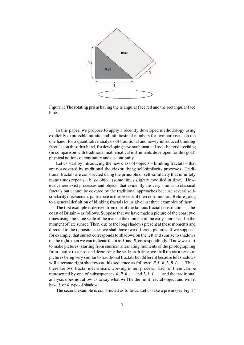
Figure 1: The rotating prism having the triangular face red and the rectangular face
blue.
In this paper, we propose to apply a recently developed methodology using
explicitly expressible infinite and infinitesimal numbers for two purposes: on the
one hand, for a quantitative analysis of traditional and newly introduced blinking
fractals; on the other hand, for developing new mathematical tools better describing
(in comparison with traditional mathematical instruments developed for this goal)
physical notions of continuity and discontinuity.
Let us start by introducing the new class of objects – blinking fractals – that
are not covered by traditional theories studying self-similarity processes. Tradi-
tional fractals are constructed using the principle of self-similarity that infinitely
many times repeats a basic object (some times slightly modified in time). How-ever, there exist processes and objects that evidently are very similar to classical
fractals but cannot be covered by the traditional approaches because several self-
similarity mechanisms participate in the process of their construction. Before going
to a general definition of blinking fractals let us give just three examples of them.
The first example is derived from one of the famous fractal constructions – the
coast of Britain – as follows. Suppose that we have made a picture of the coast two
times using the same scale of the map: at the moment of the early sunrise and at the
moment of late sunset. Then, due to the long shadows present at these moments and
directed to the opposite sides we shall have two different pictures. If we suppose,
for example, that sunset corresponds to shadows on the left and sunrise to shadows
on the right, then we can indicate them as L and R, correspondingly. If now we startto make pictures (starting from sunrise) alternating moments of the photographing
from sunrise to sunset and decreasing the scale each time, we shall obtain a series of
pictures being very similar to traditional fractals but different because left shadows
will alternate right shadows at this sequence as follows: R, L, R, L, R, L, . . . Thus,
there are two fractal mechanisms working in our process. Each of them can be
represented by one of subsequences R, R, R, . . . and L, L, L, . . . and the traditional
analysis does not allow us to say what will be the limit fractal object and will it
have L or R type of shadow.
The second example is constructed as follows. Let us take a prism (see Fig. 1)
2
8/3/2019 Yaroslav D. Sergeyev- Blinking Fractals and their Quantitative Analysis Using Infinite and Infinitesimal Numbers
http://slidepdf.com/reader/full/yaroslav-d-sergeyev-blinking-fractals-and-their-quantitative-analysis-using 3/41
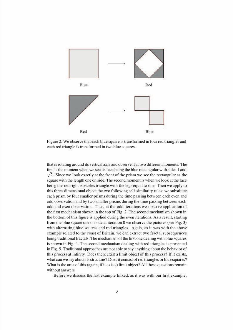
Figure 2: We observe that each blue square is transformed in four red triangles and
each red triangle is transformed in two blue squares.
that is rotating around its vertical axis and observe it at two different moments. The
first is the moment when we see its face being the blue rectangular with sides 1 and
√2. Since we look exactly at the front of the prism we see the rectangular as the
square with the length one on side. The second moment is when we look at the face
being the red right isosceles triangle with the legs equal to one. Then we apply to
this three-dimensional object the two following self-similarity rules: we substitute
each prism by four smaller prisms during the time passing between each even and
odd observation and by two smaller prisms during the time passing between each
odd and even observation. Thus, at the odd iterations we observe application of
the first mechanism shown in the top of Fig. 2. The second mechanism shown in
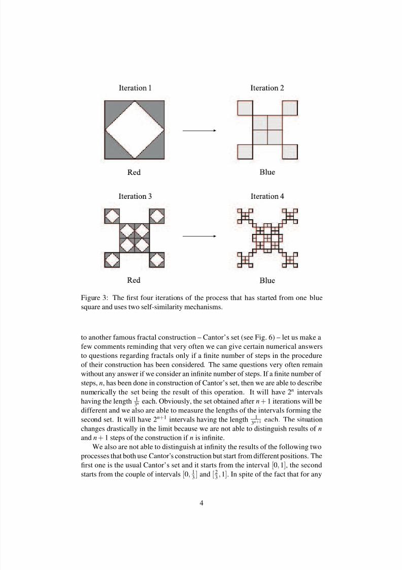
the bottom of this figure is applied during the even iterations. As a result, starting
from the blue square one on side at iteration 0 we observe the pictures (see Fig. 3)
with alternating blue squares and red triangles. Again, as it was with the above
example related to the coast of Britain, we can extract two fractal subsequences
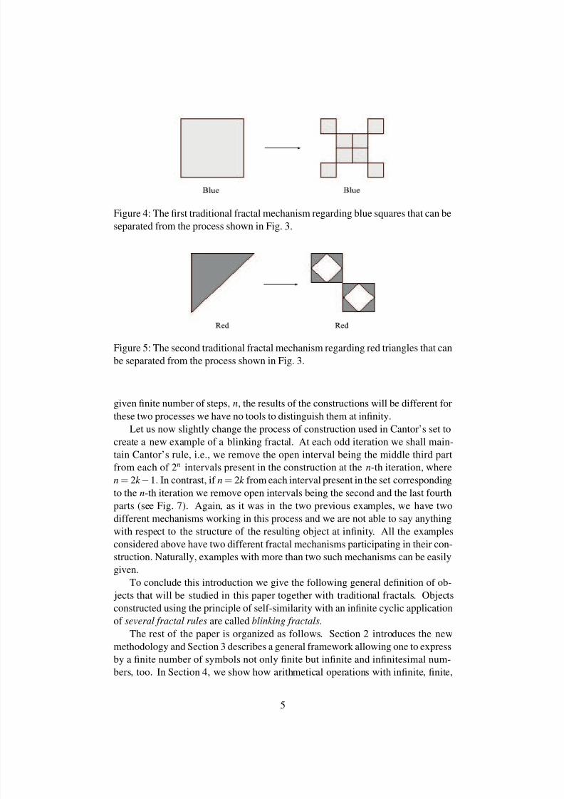
being traditional fractals. The mechanism of the first one dealing with blue squares
is shown in Fig. 4. The second mechanism dealing with red triangles is presented
in Fig. 5. Traditional approaches are not able to say anything about the behavior of
this process at infinity. Does there exist a limit object of this process? If it exists,
what can we say about its structure? Does it consist of red triangles or blue squares?
What is the area of this (again, if it exists) limit object? All these questions remain
without answers.
Before we discuss the last example linked, as it was with our first example,
3
8/3/2019 Yaroslav D. Sergeyev- Blinking Fractals and their Quantitative Analysis Using Infinite and Infinitesimal Numbers
http://slidepdf.com/reader/full/yaroslav-d-sergeyev-blinking-fractals-and-their-quantitative-analysis-using 4/41
Figure 3: The first four iterations of the process that has started from one bluesquare and uses two self-similarity mechanisms.
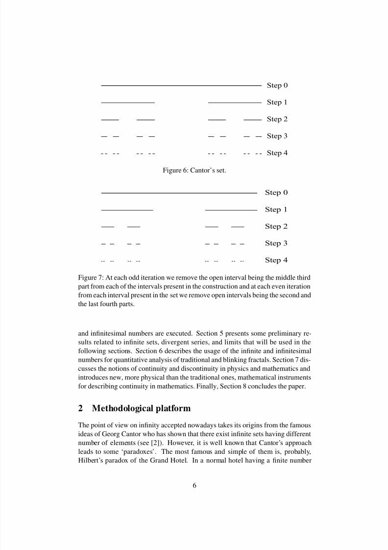
to another famous fractal construction – Cantor’s set (see Fig. 6) – let us make a
few comments reminding that very often we can give certain numerical answers
to questions regarding fractals only if a finite number of steps in the procedure
of their construction has been considered. The same questions very often remain
without any answer if we consider an infinite number of steps. If a finite number of
steps, n, has been done in construction of Cantor’s set, then we are able to describe
numerically the set being the result of this operation. It will have 2n intervals
having the length 13n each. Obviously, the set obtained after n + 1 iterations will be
different and we also are able to measure the lengths of the intervals forming the
second set. It will have 2n+1 intervals having the length 1
3n+1each. The situation
changes drastically in the limit because we are not able to distinguish results of n
and n + 1 steps of the construction if n is infinite.
We also are not able to distinguish at infinity the results of the following two
processes that both use Cantor’s construction but start from different positions. The
first one is the usual Cantor’s set and it starts from the interval [0, 1], the second
starts from the couple of intervals [0, 13
] and [23
, 1]. In spite of the fact that for any
4
8/3/2019 Yaroslav D. Sergeyev- Blinking Fractals and their Quantitative Analysis Using Infinite and Infinitesimal Numbers
http://slidepdf.com/reader/full/yaroslav-d-sergeyev-blinking-fractals-and-their-quantitative-analysis-using 5/41
Figure 4: The first traditional fractal mechanism regarding blue squares that can be
separated from the process shown in Fig. 3.
Figure 5: The second traditional fractal mechanism regarding red triangles that can
be separated from the process shown in Fig. 3.
given finite number of steps, n, the results of the constructions will be different for
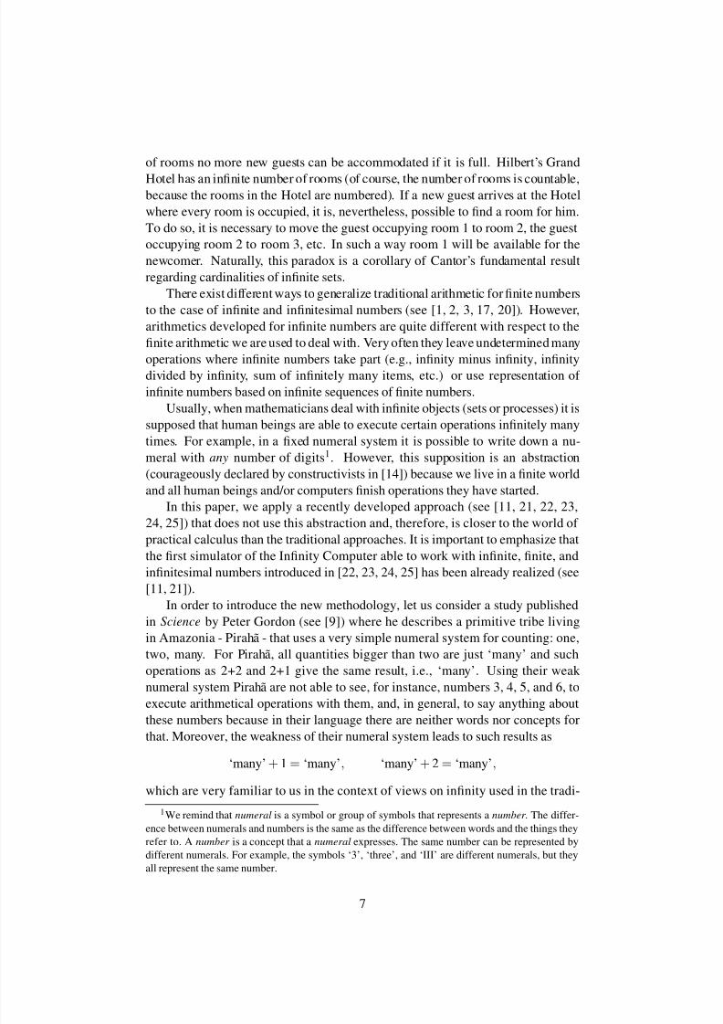
these two processes we have no tools to distinguish them at infinity.Let us now slightly change the process of construction used in Cantor’s set to
create a new example of a blinking fractal. At each odd iteration we shall main-
tain Cantor’s rule, i.e., we remove the open interval being the middle third part
from each of 2n intervals present in the construction at the n-th iteration, where
n = 2k −1. In contrast, if n = 2k from each interval present in the set corresponding
to the n-th iteration we remove open intervals being the second and the last fourth
parts (see Fig. 7). Again, as it was in the two previous examples, we have two
different mechanisms working in this process and we are not able to say anything
with respect to the structure of the resulting object at infinity. All the examples
considered above have two different fractal mechanisms participating in their con-
struction. Naturally, examples with more than two such mechanisms can be easilygiven.
To conclude this introduction we give the following general definition of ob-
jects that will be studied in this paper together with traditional fractals. Objects
constructed using the principle of self-similarity with an infinite cyclic application
of several fractal rules are called blinking fractals.
The rest of the paper is organized as follows. Section 2 introduces the new
methodology and Section 3 describes a general framework allowing one to express
by a finite number of symbols not only finite but infinite and infinitesimal num-
bers, too. In Section 4, we show how arithmetical operations with infinite, finite,
5
8/3/2019 Yaroslav D. Sergeyev- Blinking Fractals and their Quantitative Analysis Using Infinite and Infinitesimal Numbers
http://slidepdf.com/reader/full/yaroslav-d-sergeyev-blinking-fractals-and-their-quantitative-analysis-using 6/41
Step 0
Step 1
Step 2
Step 3
Step 4
Figure 6: Cantor’s set.
Step 0
Step 1
Step 2
Step 3
Step 4
Figure 7: At each odd iteration we remove the open interval being the middle third
part from each of the intervals present in the construction and at each even iterationfrom each interval present in the set we remove open intervals being the second and
the last fourth parts.
and infinitesimal numbers are executed. Section 5 presents some preliminary re-
sults related to infinite sets, divergent series, and limits that will be used in the
following sections. Section 6 describes the usage of the infinite and infinitesimal
numbers for quantitative analysis of traditional and blinking fractals. Section 7 dis-
cusses the notions of continuity and discontinuity in physics and mathematics and
introduces new, more physical than the traditional ones, mathematical instruments
for describing continuity in mathematics. Finally, Section 8 concludes the paper.
2 Methodological platform
The point of view on infinity accepted nowadays takes its origins from the famous
ideas of Georg Cantor who has shown that there exist infinite sets having different
number of elements (see [2]). However, it is well known that Cantor’s approach
leads to some ‘paradoxes’. The most famous and simple of them is, probably,
Hilbert’s paradox of the Grand Hotel. In a normal hotel having a finite number
6
8/3/2019 Yaroslav D. Sergeyev- Blinking Fractals and their Quantitative Analysis Using Infinite and Infinitesimal Numbers
http://slidepdf.com/reader/full/yaroslav-d-sergeyev-blinking-fractals-and-their-quantitative-analysis-using 7/41
of rooms no more new guests can be accommodated if it is full. Hilbert’s Grand
Hotel has an infinite number of rooms (of course, the number of rooms is countable,because the rooms in the Hotel are numbered). If a new guest arrives at the Hotel
where every room is occupied, it is, nevertheless, possible to find a room for him.
To do so, it is necessary to move the guest occupying room 1 to room 2, the guest
occupying room 2 to room 3, etc. In such a way room 1 will be available for the
newcomer. Naturally, this paradox is a corollary of Cantor’s fundamental result
regarding cardinalities of infinite sets.
There exist different ways to generalize traditional arithmetic for finite numbers
to the case of infinite and infinitesimal numbers (see [1, 2, 3, 17, 20]). However,
arithmetics developed for infinite numbers are quite different with respect to the
finite arithmetic we are used to deal with. Very often they leave undetermined many
operations where infinite numbers take part (e.g., infinity minus infinity, infinitydivided by infinity, sum of infinitely many items, etc.) or use representation of
infinite numbers based on infinite sequences of finite numbers.
Usually, when mathematicians deal with infinite objects (sets or processes) it is
supposed that human beings are able to execute certain operations infinitely many
times. For example, in a fixed numeral system it is possible to write down a nu-
meral with any number of digits1. However, this supposition is an abstraction
(courageously declared by constructivists in [14]) because we live in a finite world
and all human beings and/or computers finish operations they have started.
In this paper, we apply a recently developed approach (see [11, 21, 22, 23,
24, 25]) that does not use this abstraction and, therefore, is closer to the world of
practical calculus than the traditional approaches. It is important to emphasize thatthe first simulator of the Infinity Computer able to work with infinite, finite, and
infinitesimal numbers introduced in [22, 23, 24, 25] has been already realized (see
[11, 21]).
In order to introduce the new methodology, let us consider a study published
in Science by Peter Gordon (see [9]) where he describes a primitive tribe living
in Amazonia - Piraha - that uses a very simple numeral system for counting: one,
two, many. For Piraha, all quantities bigger than two are just ‘many’ and such
operations as 2+2 and 2+1 give the same result, i.e., ‘many’. Using their weak
numeral system Piraha are not able to see, for instance, numbers 3, 4, 5, and 6, to
execute arithmetical operations with them, and, in general, to say anything about
these numbers because in their language there are neither words nor concepts forthat. Moreover, the weakness of their numeral system leads to such results as
‘many’ + 1 = ‘many’, ‘many’ + 2 = ‘many’,
which are very familiar to us in the context of views on infinity used in the tradi-
1We remind that numeral is a symbol or group of symbols that represents a number . The differ-
ence between numerals and numbers is the same as the difference between words and the things they
refer to. A number is a concept that a numeral expresses. The same number can be represented by
different numerals. For example, the symbols ‘3’, ‘three’, and ‘III’ are different numerals, but they
all represent the same number.
7
8/3/2019 Yaroslav D. Sergeyev- Blinking Fractals and their Quantitative Analysis Using Infinite and Infinitesimal Numbers
http://slidepdf.com/reader/full/yaroslav-d-sergeyev-blinking-fractals-and-their-quantitative-analysis-using 8/41
tional calculus
∞+ 1 = ∞, ∞+ 2 = ∞.
This observation leads us to the following idea: Probably our difficulty in working
with infinity is not connected to the nature of infinity but is a result of inadequate
numeral systems used to express numbers.
We start by introducing three postulates that will fix our methodological po-
sitions with respect to infinite and infinitesimal quantities and to mathematics, in
general.
Postulate 1. We postulate existence of infinite and infinitesimal objects but
accept that human beings and machines are able to execute only a finite number of
operations.
Thus, we accept that we shall never be able to give a complete description of
infinite processes and sets due to our finite capabilities. Particularly, this means
that we accept that we are able to write down only a finite number of symbols to
express numbers.
The second postulate that will be adopted is due to the following consideration.
In natural sciences, researchers use tools to describe the object of their study and
the used instrument influences results of observations. When physicists see a black
dot in their microscope they cannot say: The object of observation is the black dot.
They are obliged to say: the lens used in the microscope allows us to see the black
dot and it is not possible to say anything more about the nature of the object of
observation until we’ll not change the instrument - the lens or the microscope itself
- by a more precise one.
Due to Postulate 1, the same happens in mathematics studying natural phe-
nomena, numbers, and objects that can be constructed by using numbers. Numeral
systems used to express numbers are among the instruments of observations used
by mathematicians. Usage of powerful numeral systems gives possibility to obtain
more precise results in mathematics in the same way as usage of a good micro-
scope gives a possibility to obtain more precise results in physics. However, the
capabilities of the tools will be always limited due to Postulate 1. Thus, following
natural sciences, we accept the second postulate.
Postulate 2. We shall not tell what are the mathematical objects we deal with;
we just shall construct more powerful tools that will allow us to improve our ca-
pacities to observe and to describe properties of mathematical objects.Particularly, this means that from our point of view, axiomatic systems do not
define mathematical objects but just determine formal rules for operating with cer-
tain numerals reflecting some properties of the studied mathematical objects.
After all, we want to treat infinite and infinitesimal numbers in the same manner
as we are used to deal with finite ones, i.e., by applying the philosophical principle
of Ancient Greeks ‘The part is less than the whole’. This principle, in our opinion,
very well reflects organization of the world around us but is not incorporated in
many traditional infinity theories where it is true only for finite numbers. Due to
this postulate, the traditional point of view on infinity accepting such results as
8

8/3/2019 Yaroslav D. Sergeyev- Blinking Fractals and their Quantitative Analysis Using Infinite and Infinitesimal Numbers
http://slidepdf.com/reader/full/yaroslav-d-sergeyev-blinking-fractals-and-their-quantitative-analysis-using 9/41
∞+ 1 = ∞ should be substituted in such a way that ∞+ 1 > ∞. Such a substitution
has several motivations: one of them can be found in [23], another one has beenintroduced in connection with the numerals of Piraha, and now we present one
more reason.
Suppose that we are at a point A and at another point, B, being infinitely far
from A there is an object. Then, if this object will change its position and will
move, let say one meter farther, we shall not be able to register this movement in a
quantitative way if we use the traditional rule ∞+ 1 =∞ to work with infinity. This
rule allows us to say only that the object was infinitely far before the movement and
remains to be infinitely far after the movement. In practice, due to this traditional
rule, we are forced to negate local movements of objects if they are infinitely far
from the observer. In order to avoid similar situations, we introduce the following
postulate that, among other things, will allow us to register local movements of objects independently on their location with respect to the origin of the coordinate
system.
Postulate 3. We adopt the principle ‘The part is less than the whole’ to all
numbers (finite, infinite, and infinitesimal) and to all sets and processes (finite and
infinite).
Due to this declared applied statement fixed by the three postulates introduced
above, such concepts as bijection, numerable and continuum sets, cardinal and or-
dinal numbers cannot be used in this paper because they belong to the theories
working with different assumptions2. On dependence of the nature of each con-
crete problem, the user will make a decision which methodology (the traditional
one or the new approach presented in this paper) better suits the problem underconsideration and will choose the respective mathematical tools. To conclude this
section, it is worthwhile to notice that the approach proposed here does not contra-
dict Cantor. In contrast, it evolves his deep ideas regarding existence of different
infinite numbers in a more applied way giving them a more quantitative character.
3 Theoretical background
Let us start our consideration by studying situations arising in practice when it is
necessary to operate with extremely large quantities (see [22] for a detailed discus-
sion). Imagine that we are in a granary and the owner asks us to count how much
grain he has inside it. There are a few possibilities of finding an answer to this
question. The first one is to count the grain seed by seed. Of course, nobody can
do this because the number of seeds is enormous.
To overcome this difficulty, people take sacks, fill them in with seeds, and
count the number of sacks. It is important that nobody counts the number of seeds
in a sack. At the end of the counting procedure, we shall have a number of sacks
completely filled and some remaining seeds that are not sufficient to complete the
2As a consequence, the approach used in this paper is different also with respect to the non-
standard analysis introduced in [20] and built using Cantor’s ideas.
9
8/3/2019 Yaroslav D. Sergeyev- Blinking Fractals and their Quantitative Analysis Using Infinite and Infinitesimal Numbers
http://slidepdf.com/reader/full/yaroslav-d-sergeyev-blinking-fractals-and-their-quantitative-analysis-using 10/41
next sack. At this moment it is possible to return to the seeds and to count the
number of remaining seeds that have not been put in sacks (or a number of seedsthat it is necessary to add to obtain the last completely full sack).
If the granary is huge and it becomes difficult to count the sacks, then trucks
or even big train waggons are used. Of course, we suppose that all sacks contain
the same number of seeds, all trucks – the same number of sacks, and all waggons
– the same number of trucks. At the end of the counting we obtain a result in the
following form: the granary contains 16 waggons, 13 trucks, 12 sacks, and 4 seeds
of grain. Note, that if we add, for example, one seed to the granary, we can count
it and see that the granary has more grain. If we take out one waggon, we again be
able to say how much grain has been subtracted.
Thus, in our example it is necessary to count large quantities. They are fi-
nite but it is impossible to count them directly using elementary units of measure,u0, i.e., seeds, because the quantities expressed in these units would be too large.
Therefore, people are forced to behave as if the quantities were infinite.
To solve the problem of ‘infinite’ quantities, new units of measure, u1, u2, and
u3, are introduced (units u1 – sacks, u2 – trucks, and u3 – waggons). The new
units have the following important peculiarity: it is not known how many units ui
there are in the unit ui+1 (we do not count how many seeds are in a sack, we just
complete the sack). Every unit ui+1 is filled in completely by the units ui. Thus, we
know that all the units ui+1 contain a certain number K i of units ui but this number,
K i, is unknown. Naturally, it is supposed that K i is the same for all instances of
the units. Thus, numbers that it was impossible to express using only initial units
of measure are perfectly expressible if new units are introduced. This key idea of counting by introduction of new units of measure will be used in the paper to deal
with infinite quantities.
Different numeral systems have been developed by humanity to describe finite
numbers. More powerful numeral systems allow us to write down more numerals
and, therefore, to express more numbers. In order to have a possibility to write
down infinite and infinitesimal numbers by a finite number of symbols, we need at
least one new numeral expressing an infinite (or an infinitesimal) number. Then, it
is necessary to propose a new numeral system fixing rules for writing down infinite
and infinitesimal numerals and to describe arithmetical operations with them.
Note that introduction of a new numeral for expressing infinite and infinites-
imal numbers is similar to introduction of the concept of zero and the numeral‘0’ that in the past have allowed people to develop positional systems being more
powerful than numeral systems existing before.
In positional numeral systems fractional numbers are expressed by the record
(anan−1 . . . a1a0.a−1a−2 . . . a−(q−1)a−q)b (1)
where numerals ai,−q≤ i≤ n, are called digits, belong to the alphabet 0, 1, . . . , b−1, and the dot is used to separate the fractional part from the integer one. Thus,
10
8/3/2019 Yaroslav D. Sergeyev- Blinking Fractals and their Quantitative Analysis Using Infinite and Infinitesimal Numbers
http://slidepdf.com/reader/full/yaroslav-d-sergeyev-blinking-fractals-and-their-quantitative-analysis-using 11/41
the numeral (1) is equal to the sum
anbn + an−1bn−1 + . . . + a1b1 + a0b0 + a−1b−1 + . . . + a−(q−1)b
−(q−1) + a−qb−q.(2)
In modern computers, the radix b = 2 with the alphabet 0, 1 is mainly used to
represent numbers. Numerous ways to represent and to store numbers in computers
are described, for example, in [16].
Record (1) uses numerals consisting of one symbol each, i.e., digits ai ∈ 0, 1,. . . , b− 1, to express how many finite units of the type bi belong to the number
(2). Quantities of finite units bi are counted separately for each exponent i and all
symbols in the alphabet 0, 1, . . . , b−1 express finite numbers.
A new positional numeral system with infinite radix described in this section
evolves the idea of separate count of units with different exponents used in tradi-tional positional systems to the case of infinite and infinitesimal numbers. The infi-
nite radix of the new system is introduced as the number of elements of the setN of
natural numbers expressed by the numeral x called grossone. This mathematical
object is introduced by describing its properties postulated by the Infinite Unit Ax-
iom consisting of three parts: Infinity, Identity, and Divisibility (we introduce them
soon). This axiom is added to axioms for real numbers similarly to addition of the
axiom determining zero to axioms of natural numbers when integer numbers are
introduced. This means that it is postulated that associative and commutative prop-
erties of multiplication and addition, distributive property of multiplication over
addition, existence of inverse elements with respect to addition and multiplication
hold for grossone as for finite numbers.Note that usage of a numeral indicating totality of the elements we deal with is
not new in mathematics. It is sufficient to remind the theory of probability where
events can be defined in two ways. First, as union of elementary events; second, as
a sample space, Ω, of all possible elementary events from where some elementary
events have been excluded. Naturally, the second way to define events becomes
particularly useful when the sample space consists of infinitely many elementary
events.
The Infinite Unit Axiom consists of the following three statements:
Infinity. For any finite natural number n it follows n < x.
Identity. The following relations link x to identity elements 0 and 1
0 ·x=x ·0 = 0, x−x= 0,x
x= 1, x
0 = 1, 1x= 1, 0x= 0. (3)
Divisibility. For any finite natural number n sets Nk ,n, 1 ≤ k ≤ n, being the nth
parts of the set, N, of natural numbers have the same number of elements
indicated by the numeral xn
where
Nk ,n = k , k + n, k + 2n, k + 3n, . . ., 1≤ k ≤ n,n
k =1
Nk ,n = N. (4)
11

8/3/2019 Yaroslav D. Sergeyev- Blinking Fractals and their Quantitative Analysis Using Infinite and Infinitesimal Numbers
http://slidepdf.com/reader/full/yaroslav-d-sergeyev-blinking-fractals-and-their-quantitative-analysis-using 12/41
Divisibility is based on Postulate 3. Let us illustrate it by three examples. If we take
n = 1, thenN1,1 =N and Divisibility tells that the set, N, of natural numbers hasxelements. If n = 2, we have two sets N1,2 andN2,2 and they have x
2elements each.
If n = 3, then we have three sets N1,3, N2,3, and N3,3 and they have x3
elements
each.
x→ N= 1, 2, 3, 4, 5, 6, 7, . . .
x
2
N1,2 = 1, 3, 5, 7, . . .
N2,2 = 2, 4, 6, . . .
x
3→
N1,3 = 1, 4, 7, . . .
N2,3 = 2, 5, . . .
N3,3 = 3, 6, . . .
Before the introduction of the new positional system let us study some prop-
erties of grossone. First of all, as was already mentioned above, it is necessary to
remind that x is not either Cantor’s ℵ0 or ω that have been introduced in Can-
tor’s theory on the basis of different assumptions. It will be shown hereinafter that
grossone unifies both cardinal and ordinal aspects in the same way as finite nu-
merals unify them. Its role in our infinite arithmetic is similar to the role of the
number 1 in the finite arithmetic and it will serve us as the basis for construction of
other infinite and infinitesimal numbers.
We start by the following important comment: to introduce xn
we do not try
to count elements k , k + n, k + 2n, k + 3n, . . . In fact, we cannot do this due to the
accepted Postulate 1. In contrast, we apply Postulate 3 and state that the number
of elements of the nth part of the set, i.e., xn
, is n times less than the number of
elements of the whole set, i.e., than x. In terms of our granary example x can be
interpreted as the number of seeds in the sack. Then, if the sack contains x seeds,
its nth part contains xn
seeds. It is worthy to emphasize that, since the numbers xn
have been introduced as numbers of elements of sets Nk ,n, they are integer.
The introduced numerals xn
and the sets Nk ,n allow us immediately to calculate
the number of elements of certain infinite sets. For example, due to the introducedaxiom, the sets
N4,5 = 4, 9, 14, 19, 24, 29, 34, 39, 44, 49, 54, 59, 64, 69, 74, 79, . . .
N3,11 = 3, 14, 25, 36, 47, 58, 69, 80, 91, 102, 113, 124, 135, . . .,
have x5
and x11
elements, correspondingly.
The number of elements of sets being union, intersection, difference, or prod-
uct of other sets of the type Nk ,n is defined in the same way as these operations are
defined for finite sets. Thus, we can define the number of elements of sets being
12
8/3/2019 Yaroslav D. Sergeyev- Blinking Fractals and their Quantitative Analysis Using Infinite and Infinitesimal Numbers
http://slidepdf.com/reader/full/yaroslav-d-sergeyev-blinking-fractals-and-their-quantitative-analysis-using 13/41
results of these operations with finite sets and infinite sets of the type Nk ,n. Let us
consider three simple examples (a general rule for determining the number of ele-ments of infinite sets having a more complex structure will be given in Section 5).
First, we study intersection of the sets N4,5 and N3,11. It follows from the axiom
that
N4,5∩N3,11 = 14, 69, 124, . . .= N14,55
and, therefore, it has x55
elements. In the second example we consider the set
N4,5∪2, 3, 4. Its number of elements is x5
+ 2 because 4 ∈N4,5.
It is worthwhile to notice that, as it is for finite sets, operations of union and
intersection with finite sets and infinite sets of the type Nk ,n enjoy commutative
property. Thus, in our example we have
N4,5∩N3,11 = N3,11∩N4,5,
N4,5∪2, 3, 4= 2, 3, 4∪N4,5
and x5
+2 = 2+x5
. In the last example we consider the setN2,5∪3, 5\2, 7, 17.
It has x5− 1 elements because two elements have been added to and three have
been excluded from the set N2,5 = 2, 7, 12, 17, . . . having x5
elements.
Other results regarding calculating the number of elements of infinite sets can
be found in [22]. Particularly, it is shown that the number of elements of the set, Z,
of integers is equal to 2x1 and the number of elements of the set, Q, of different
rational numerals is equal to 2x
2
1. Then, Section 5 shows how to calculate thenumber of elements of infinite sets defined by formulae.
The new numeral x allows us to write down the set, N, of natural numbers in
the form
N= 1, 2, 3, . . . x−2, x−1, x (5)
because grossone has been introduced as the number of elements of the set of nat-
ural numbers (similarly, the number 3 is the number of elements of the set 1, 2,
3). Thus, grossone is the biggest natural number and infinite numbers
. . . x−3, x−2, x−1 (6)
less than grossone are also natural numbers as the numbers 1, 2, 3, . . . They can beviewed both in terms of sets of numbers and in terms of grain. For example, x−1
can be interpreted as the number of elements of the set N from which a number has
been excluded. In terms of our granary example x−1 can be interpreted as a sack
minus one seed.
Note that the set (5) is the same set of natural numbers we are used to deal with.
Infinite numbers (6) also take part of the usual set, N, of natural numbers3. The
difficulty to accept existence of infinite natural numbers is in the fact that traditional
3This point is one of the differences with respect to non-standard analysis (see [19, 20]) where
infinite numbers are not included in N.
13
8/3/2019 Yaroslav D. Sergeyev- Blinking Fractals and their Quantitative Analysis Using Infinite and Infinitesimal Numbers
http://slidepdf.com/reader/full/yaroslav-d-sergeyev-blinking-fractals-and-their-quantitative-analysis-using 14/41
numeral systems did not allow us to see them. In the same way as Piraha are not
able to see, for instance, numbers 4, 5, and 26 using their weak numeral system,traditional numeral systems did not allow us to see infinite natural numbers that we
can see now using the new numeral x.
We remind also that usage of a numeral indicating the infinite totality of the
elements we deal with is not new in mathematics. In the same way as we use x to
indicate the number of all natural numbers, in the probability theory the axiomatic
of Kolmogorov uses the symbol Ω to indicate the sample space of all possible
elementary events. Then, the events can be described as union of elementary events
or as Ω (or its parts) from where some elementary events have been excluded.
Analogously, natural numbers can be described as union of finite units or as x (or
its parts) from where some finite units have been excluded.
Now an obvious question arises: Which natural numbers can we express byusing the new numeral x? Suppose that we have a numeral system S for express-
ing finite natural numbers and it allows us to express numbers belonging to a set
N S ⊂N. Then, adding x to this numeral system will allow us to express also infi-
nite natural numbers ixn±k ≤xwhere 1≤ i≤ n, k ∈N S , n∈N S (note that since
xn
are integer, ixn
are integer too). Thus, the more powerful system S is used to ex-
press finite numbers, the more infinite numbers can be expressed. This also means
that the new numeral system using grossone allows us to express more numbers
than traditional numeral systems thanks to the introduced new numerals but, as all
numeral systems, it has a limited expressibility.
As an example, let us consider the numeral system, P , of Piraha able to express
only numbers 1 and 2 (the only difference will be in the usage of the numerals ‘1’
and ‘2’ instead of original numerals I and II used by Piraha). If we add to this
system the new numeral x it becomes possible to express the following numbers
1, 2 finite
, . . .x
2−2,
x
2−1,
x
2,x
2+ 1,
x
2+ 2
infinite
, . . . x−2,x−1,x infinite
.
In this record the first two numbers are finite, the remaining eight are infinite, and
dots show the natural numbers that are not expressible in this numeral system. This
numeral system does not allow us to execute such operation as 2 + 2 or to add 2 tox2 + 2 because their results cannot be expressed in this system but, of course, we
do not write that results of these operations are equal, we just say that the results
are not expressible in P and it is necessary to take another, more powerful numeral
system.
Note that we have similar crucial limitations working with sets. The numeral
system P allows us to define only the sets N1,2 and N2,2 among all possible sets of
the formNk ,n from (4) because we have only two finite numerals, ‘1’ and ‘2’, in P .
This numeral system is too weak to define other sets of this type. These limitations
have a general deep character and are related to all problems requiring a numerical
answer (i.e., an answer expressed only in numerals, without variables). In order to
14
8/3/2019 Yaroslav D. Sergeyev- Blinking Fractals and their Quantitative Analysis Using Infinite and Infinitesimal Numbers
http://slidepdf.com/reader/full/yaroslav-d-sergeyev-blinking-fractals-and-their-quantitative-analysis-using 15/41
obtain such an answer, it is necessary to know at least one numeral system able to
express numerals required to write down this answer.The introduction of grossone allows us to obtain the following interesting re-
sult: the set N is not a monoid under addition. In fact, the operation x+ 1 gives us
as the result a number grater than x. Thus, by definition of grossone, x+ 1 does
not belong to N and, therefore, N is not closed under addition and is not a monoid.
This result is a straightforward consequence of the accepted Postulate 3.
This result also means that adding the Infinite Unit Axiom to the axioms of
natural numbers defines the set of extended natural numbers indicated as N and
includingN as a proper subset
N= 1, 2, . . . ,x−1,x,x+ 1, . . . ,x2−1,x2,x2 + 1, . . ..
Again, extended natural numbers grater than grossone can also be interpreted in
the terms of sets of numbers. For example, x+ 3 as the number of elements of the
setN∪a, b, cwhere numbers a, b, c /∈N andx2 as the number of elements of the
set N×N. In terms of our granary example x+ 3 can be interpreted as one sack
plus three seeds and x2 as a truck if we accept that the numbers K i from page 10
are such that K 1 = K 2 =x.
Extended natural numbers can be ordered as follows
1 < 2 < ... <x−1 <x<x+ 1 < ... <x2−1 <x2 <x2 + 1 < .. .
Let us show, for instance, that x<x2. We can write the difference
x2−x=x(x−1). (7)
Due to Infinity property, x is greater than any finite natural number, therefore,
x> 1 and as a consequence x−1 > 0. It follows from this inequality and (7) that
the number x2−x is a positive number and, therefore, x2 >x.
The set, Z, of extended integer numbers can be constructed from the set Z by
a complete analogy and inverse elements with respect to addition are introduced
naturally. For example, 6x has its inverse with respect to addition equal to −6x.
We have already started to write down simple infinite numbers and to execute
arithmetical operations with them without concentrating our attention upon this
question. Let us consider it systematically.To express infinite and infinitesimal numbers we shall use records that are sim-
ilar to (1) and (2) but have some peculiarities. In order to construct a number C
in the new numeral positional system with base x we subdivide C into groups
corresponding to powers of x:
C = c pmx pm + . . . + c p1x
p1 + c p0x p0 + c p
−1x
p−1 + . . . + c p
−k x
p−k . (8)
Then, the record
C = c pmx pm . . . c p1x
p1c p0x p0c p
−1x
p−1 . . .c p
−k x
p−k (9)
15
8/3/2019 Yaroslav D. Sergeyev- Blinking Fractals and their Quantitative Analysis Using Infinite and Infinitesimal Numbers
http://slidepdf.com/reader/full/yaroslav-d-sergeyev-blinking-fractals-and-their-quantitative-analysis-using 16/41
represents the number C , where finite numbers ci are called infinite grossdigits and
can be both positive and negative; numbers pi are called grosspowers and can befinite, infinite, and infinitesimal (the introduction of infinitesimal numbers will be
given soon). The numbers pi are such that pi > 0, p0 = 0, p−i < 0 and
pm > pm−1 > .. . p2 > p1 > p−1 > p
−2 > .. . p−(k −1) > p
−k .
In the traditional record (1) there exists a convention that a digit ai shows how many
powers bi are present in the number and the radix b is not written explicitly. In the
record (9) we write x pi explicitly because in the new numeral positional system
the number i in general is not equal to the grosspower pi. This gives possibility to
write, for example, such numbers as 7x244.5 3x−32 where p1 = 244.5, p−1 =−32.
Finite numbers in this new numeral system are represented by numerals havingonly one grosspower equal to zero. In fact, if we have a number C such that m =k = 0 in representation (9), then due to (3) we have C = c0x
0 = c0. Thus, the
number C in this case does not contain infinite units and is equal to the grossdigit
c0 which being a conventional finite number can be expressed in the form (1), (2)
by any positional system with finite base b (or by another numeral system). It is
important to emphasize that the grossdigit c0 can be integer or fractional and can be
expressed by a few symbols in contrast to the traditional record (1) where each digit
is integer and is represented by one symbol from the alphabet 0, 1, 2, . . . , b− 1.
Thus, the grossdigit c0 shows how many finite units and/or parts of the finite unit,
1 =x0, belong to the number C .
Analogously, in the general case, all grossdigits ci,−k ≤ i ≤ m, can be in-teger or fractional and expressed by many symbols. For example, the number7
3x
4 84
19x−3.1 has grossdigits c4 = 7
3and c−3.1 = 84
19. All grossdigits show how many
corresponding units take part in the number C and it is not important whether this
unit is finite or infinite.
Infinite numbers with finite grosspowers in this numeral system are expressed
by numerals having at least one grosspower grater than zero. In the following
example the left-hand expression presents the way to write down infinite numbers
and the right-hand shows how the value of the number is calculated:
15x1417.2045x352.1x−6 = 15x14 + 17.2045x3 + 52.1x−6.
If a grossdigit c pi is equal to 1 then we write x pi instead of 1x pi . Analogously, if
power x0 is the lowest in a number then we often use simply the corresponding
grossdigit c0 withoutx0, for instance, we write 23x145 instead of 23x145x0 or 3
instead of 3x0. We also write sometimes x1 simply as x.
Numerals with finite grosspowers having only negative grosspowers represent
infinitesimal numbers. The simplest number from this group isx−1 = 1
xbeing the
inverse element with respect to multiplication for x:
1
x·x=x · 1
x= 1. (10)
16
8/3/2019 Yaroslav D. Sergeyev- Blinking Fractals and their Quantitative Analysis Using Infinite and Infinitesimal Numbers
http://slidepdf.com/reader/full/yaroslav-d-sergeyev-blinking-fractals-and-their-quantitative-analysis-using 17/41
Note that all infinitesimals are not equal to zero. Particularly, 1
x> 0 because 1 > 0
and x > 0. It has a clear interpretation in our granary example. Namely, if wehave a sack and it contains x seeds then one sack divided by x is equal to one
seed. Vice versa, one seed, i.e., 1
x, multiplied by the number of seeds in the sack,
x, gives one sack of seeds.
Inverse elements of more complex numbers including grosspowers of x are
defined by a complete analogy. The following two numbers are examples of infin-
itesimals 3x−32, 37x−211x−15.
The above examples show how we can write down infinite numbers with all
grossdigits being finite numbers. Let us see now how we can express a number
including infinite grossdigits. The number
−14x
2
(0.5x
+ 3)x
1
(x
−4.5)x−1
(11)has m = 2, k = 1, and the following grossdigits
c2 =−14, c1 = 0.5x+ 3, c−1 =x−4.5,
where c2 is finite and c1, c−1 are infinite. The record (11) is correct but not very
elegant because the system base x appears in the expressions of grossdigits. In
order to overcome this unpleasantness and to introduce a more simple structure of
infinite numerals, we rewrite the number (11) in the explicit form (8)
−14x2(0.5x+ 3)x1(x−4.5)x−1 =−14x2 + (0.5x+ 3)x1 + (x−4.5)x−1.
Then we open the parenthesis, collect the items having the same powers of x
(taking into account that xx−1 =x0), and finally obtain
−14x2 + (0.5x+ 3)x1 + (x−4.5)x−1 =
−14x2 + 0.5x2 + 3x1 +xx−1−4.5x−1 =
−13.5x2 + 3x1 +x0−4.5x−1 =−13.5x23x1x
0(−4.5)x−1. (12)
As can be seen from the record (12), there are no infinite grossdigits in it but
negative grossdigits have appeared. Since the record (11) using infinite grossdigits
is more cumbersome, we introduce the notion of finite grossdigit as a finite number
ci expressed by a finite number of symbols in a numeral system and showing how
many infinite units of the type xk i ,−
k
≤i
≤m, should be added or subtracted in
order to compose infinite numbers. The record (12) using finite grossdigits is more
flexible than the record (11) and will be mainly used hereinafter to express infinite
and infinitesimal numbers.
4 Arithmetical operations for infinite, infinitesimal, and
finite numbers
Let us now introduce arithmetical operations for infinite, infinitesimal, and finite
numbers. The operation of addition of two given infinite numbers A and B returns
17
8/3/2019 Yaroslav D. Sergeyev- Blinking Fractals and their Quantitative Analysis Using Infinite and Infinitesimal Numbers
http://slidepdf.com/reader/full/yaroslav-d-sergeyev-blinking-fractals-and-their-quantitative-analysis-using 18/41
as the result an infinite number C constructed as follows (the operation of subtrac-
tion is a direct consequence of that of addition and is thus omitted). The numbers A, B, and their sum C are represented in the record of the type (12):
A =K
∑i=1
ak ixk i , B =
M
∑ j=1
bm jx
m j , C = L
∑i=1
clixli . (13)
Then the result C is constructed by including in it all items ak ixk i from A such that
k i = m j, 1 ≤ j ≤ M , and all items bm jx
m j from B such that m j = k i, 1 ≤ i ≤ K . If
in A and B there are items such that k i = m j for some i and j then this grosspower
k i is included in C with the grossdigit bk i + ak i , i.e., as (bk i + ak i)xk i . It can be
seen from this definition that the introduced operation enjoys the usual properties
of commutativity and associativity due to definition of grossdigits and the fact thataddition for each grosspower of x is executed separately.
Let us illustrate the rules by an example (in order to simplify the presentation in
all the following examples the radix b = 10 is used for writing down grossdigits).
We consider two infinite numbers A and B where
A = 16.5x44.2(−12)x1217x01.17x−3,
B = 23x146.23x310.1x0(−1.17)x−311x−43.
Their sum C is calculated as follows
C = A + B = 16.5x44
.2
+ (−12)x12
+ 17x0
+ 1.17x−3
+
23x14 + 6.23x3 + 10.1x0−1.17x−3 + 11x−43 =
16.5x44.2 + 23x14−12x12 + 6.23x3+
(17 + 10.1)x0 + (1.17−1.17)x−3 + 11x−43 =
16.5x44.2 + 23x14−12x12 + 6.23x3 + 27.1x0 + 11x−43 =
16.5x44.223x14(−12)x126.23x327.1x011x−43.
The operation of multiplication of two given infinite numbers A and B from
(13) returns as the result the infinite number C constructed as follows.
C = M
∑ j=1
C j, C j = bm jx
m j · A =K
∑i=1
ak ibm jx
k i+m j , 1≤ j ≤ M . (14)
Similarly to addition, the introduced multiplication is commutative and associative.
It is easy to show that the distributive property is also valid for these operations.
Let us illustrate this operation by the following example. We consider two
infinite numbers
A =x18(−5)x2(−3)x10.2, B =x2(−1)x17x−3
18
8/3/2019 Yaroslav D. Sergeyev- Blinking Fractals and their Quantitative Analysis Using Infinite and Infinitesimal Numbers
http://slidepdf.com/reader/full/yaroslav-d-sergeyev-blinking-fractals-and-their-quantitative-analysis-using 19/41
and calculate the product C = B
· A. The first partial product C 1 is equal to
C 1 = 7x−3 · A = 7x−3(x18−5x2−3x1 + 0.2) =
7x15−35x−1−21x−2 + 1.4x−3 = 7x15(−35)x−1(−21)x−21.4x−3.
The other two partial products, C 2 and C 3, are computed analogously:
C 2 =−x1 · A =−x1(x18−5x2−3x1 + 0.2) =−x195x33x2(−0.2)x1,
C 3 =x2 · A =x2(x18−5x2−3x1 + 0.2) =x20(−5)x4(−3)x30.2x2.
Finally, by taking into account that grosspowers x3 and x2 belong to both C 2and C 3 and, therefore, it is necessary to sum up the corresponding grossdigits, the
product C is equal (due to its length, the number C is written in two lines) to
C = C 1 +C 2 +C 3 = x20(−1)x197x15(−5)x42x33.2x2
(−0.2)x1(−35)x−1(−21)x−21.4x−3.
In the operation of division of a given infinite number C by an infinite number
B we obtain an infinite number A and a reminder R that can be also equal to zero,
i.e., C = A · B + R.
The number A is constructed as follows. The numbers B and C are represented
in the form (13). The first grossdigit ak K and the corresponding maximal exponent
k K are established from the equalities
ak K = cl L/bm M , k K = l L−m M . (15)
Then the first partial reminder R1 is calculated as
R1 = C −ak K xk K · B. (16)
If R1 = 0 then the number C is substituted by R1 and the process is repeated by a
complete analogy. The grossdigit ak K −i , the corresponding grosspower k K −i and the
partial reminder Ri+1 are computed by formulae (17) and (18) obtained from (15)
and (16) as follows: l L and cl L are substituted by the highest grosspower ni and the
corresponding grossdigit r ni of the partial reminder Ri that in its turn substitutes C :
ak K −i = r ni/bm M , k K −i = ni−m M . (17)
Ri+1 = Ri−ak K −ixk K −i · B, i ≥ 1. (18)
The process stops when a partial reminder equal to zero is found (this means that
the final reminder R = 0) or when a required accuracy of the result is reached.
The operation of division will be illustrated by two examples. In the first ex-
ample we divide the number C = −10x316x042x−3 by the number B = 5x37.
For these numbers we have
l L = 3, m M = 3, cl L =−10, bm M = 5.
19
8/3/2019 Yaroslav D. Sergeyev- Blinking Fractals and their Quantitative Analysis Using Infinite and Infinitesimal Numbers
http://slidepdf.com/reader/full/yaroslav-d-sergeyev-blinking-fractals-and-their-quantitative-analysis-using 20/41
It follows immediately from (15) that ak K xk K =
−2x0. The first partial reminder
R1 is calculated as
R1 =−10x316x042x−3− (−2x0) ·5x37 =
−10x316x042x−3 + 10x314x0 = 30x042x−3.
By a complete analogy we should construct ak K −1xk K −1 by rewriting (15) for R1.
By doing so we obtain equalities
30 = ak K −1 ·5, 0 = k K −1 + 3
and, as the result, ak K −1xk K −1 = 6x−3. The second partial reminder is
R2 = R1−6x−3 ·5x37 = 30x042x−3−30x042x−3 = 0.
Thus, we can conclude that the reminder R = R2 = 0 and the final result of division
is A =−2x06x−3.
Let us now substitute the grossdigit 42 by 40 in C and divide this new numberC = −10x316x040x−3 by the same number B = 5x37. This operation gives us
the same result A2 = A =−2x06x−3 (where subscript 2 indicates that two partial
reminders have been obtained) but with the reminder R = R2 = −2x−3. Thus,
we obtain C = B · A2 + R2. If we want to continue the procedure of division, we
obtain
A3 = −2x06x−3(−0.4)x−6 with the reminder
R3 = 0.28x−6. Naturally,
it follows C = B
· A3 + R3. The process continues until a partial reminder Ri = 0 is
found or when a required accuracy of the result will be reached.In all the examples above we have used grosspowers being finite numbers.
However, all the arithmetical operations work by a complete analogy also for
grosspowers being themselves numbers of the type (9). For example, if
X = 16.5x44.2x1.17x−3
(−12)x12x1.17x−3,
Y = 23x44.2x1.17x−3
(−1.17)x−311x4x−23
,
then their sum Z is calculated as follows
Z = X +Y = 39.5x
44.2x1.17x−3
(−12)x
12x
11x
4x−23
.
5 Preliminary results
We start this section by showing how a number of elements of an infinite set can be
determined in case when its elements are defined by a formula. We have already
discussed in Section 3 how we can do this for sets being results of the usual oper-
ations (intersection, union, etc.) with finite sets and infinite sets of the type Nk ,n.
In order to have a possibility to construct more complex infinite sets using these
operations and to be able to determine the number of elements of the resulting
20
8/3/2019 Yaroslav D. Sergeyev- Blinking Fractals and their Quantitative Analysis Using Infinite and Infinitesimal Numbers
http://slidepdf.com/reader/full/yaroslav-d-sergeyev-blinking-fractals-and-their-quantitative-analysis-using 21/41
sets, let us consider infinite sets having a more general structure than the sets Nk ,n.
Suppose that we have an integer function f (i) > 0 strictly increasing on indexesi = 1, 2, 3, . . . and we wish to know how many elements are there in the set
F = f (1), f (2), f (3), . . ..
In our terminology this question has no any sense because due to Postulate 3 the
set F is not defined completely. Let us explain what does this mean.
In the finite case, to define a set it is not sufficient to say that it is finite. It is
necessary to indicate explicitly or implicitly its number of elements. For example,
F 1 = f (i) : 1 ≤ i ≤ 10
or
F 2 = f (i) : i≥ 1, f (i)≤ awhere a is finite.
Now we have mathematical tools to indicate the number of elements for infinite
sets, too. Thus, analogously to the finite case and due to Postulate 3, to define a set
it is not sufficient to say that the set has infinitely many elements. It is necessary to
indicate its number of elements explicitly or implicitly. In the following example,
the number of elements of the set
F 1 =
f (i) : 1
≤i
≤
x2
2+ 1
is indicated explicitly. It has x
2
2+ 1 elements. Analogously, the number of el-
ements of the set, N, of natural numbers has been indicated explicitly (see the
Infinite Unit Axiom, Divisibility)
N= i : 1 ≤ i≤x
The number of elements of the set
F 2 = f (i) : i≥ 1, f (i)≤ b (19)
where b is infinite, is defined implicitly (particularly, if b =x
then the set F ⊆ Nsince all its elements are integer, positive, and f (i)≤x). In both cases, finite and
infinite, it is necessary to have numeral systems allowing us to express numbers a
and b.
If a set is given in the form (19), then its number of elements J can be deter-
mined as
J = maxi : f (i)≤ b.
If we are able to determine the inverse function f −1( x) for f ( x) then J = [ f −1(b)]where [u] is integer part of u.
21
8/3/2019 Yaroslav D. Sergeyev- Blinking Fractals and their Quantitative Analysis Using Infinite and Infinitesimal Numbers
http://slidepdf.com/reader/full/yaroslav-d-sergeyev-blinking-fractals-and-their-quantitative-analysis-using 22/41
Let us consider as examples two subsets of N depending on finite and integer
parameters k and n. The first set, F 1, has f (i) = k + n(i−1). Then
F 1 = f (i) : i≥ 1, f (i)≤x= Nk ,n, 1≤ k ≤ n,
where Nk ,n is from (4). It has J 1 elements where
J 1 = [x− k
n+ 1] = [
x− k
n] + 1 =
x
n−1 + 1 =
x
n.
Analogously, the second set
F 2 = k + ni3 : i≥ 1, k + ni3 ≤x
has J 2 = [3 x−k
n] elements.
What can we say now about the number of elements of the sets N and Z?
Our positional numeral system with the radix x dose not allow us to say anything
because it does not contain numerals able to express such numbers. It is necessary
to introduce in a way a more powerful numeral system defining new numerals y,
z, etc. However, we can work with those subsets of N and Z that can be defined by
using numerals written down in our positional numeral system with the radix x.
In order to have a possibility to discuss such important constructions as recur-
sively defined infinite sets we need first to consider infinite sequences from the
point of view of the new approach.
We start by proving the following important result: the number of elements of any infinite sequence is less or equal to x. To demonstrate this we need to recall
the definition of the infinite sequence: ‘An infinite sequence an, an ∈ A for all
n ∈N, is a function having as the domain the set of natural numbers, N, and as the
codomain a set A’.
We have postulated in the Infinite Unit Axiom that the set N has x elements.
Thus, due to the sequence definition given above, any sequence having N as the
domain has x elements.
One of the immediate consequences of the understanding of this result is that
any process can have at maximum x elements. For example, if we consider the
set, N, of extended natural numbers then starting from the number 1, it is possible
to arrive at maximum to x
1, 2, 3, 4, . . . x−2, x−1,x x
,x+ 1,x+ 2,x+ 3, . . . (20)
Starting from 2 it is possible to arrive at maximum to x+ 1
1, 2, 3, 4, . . . x−2, x−1,x,x+ 1 x
,x+ 2,x+ 3, . . . (21)
22
8/3/2019 Yaroslav D. Sergeyev- Blinking Fractals and their Quantitative Analysis Using Infinite and Infinitesimal Numbers
http://slidepdf.com/reader/full/yaroslav-d-sergeyev-blinking-fractals-and-their-quantitative-analysis-using 23/41
Starting from 3 it is possible to to arrive at maximum to x+ 2
1, 2, 3, 4, . . . x−2, x−1,x,x+ 1,x+ 2 x
,x+ 3, . . . (22)
Of course, since we have postulated that our possibilities to express numerals are
finite, it depends on the chosen numeral system which numbers among xmembers
of these processes we can observe. It is also very important to notice a deep relation
of this observation to the Axiom of Choice. The Infinite Unit Axiom postulates
that any process can have at maximum x elements, thus the process of choice too
and, as a consequence, it is not possible to choose more than x elements from
a set. This observation also emphasizes the fact that the parallel computational
paradigm is significantly different with respect to the sequential one because pparallel processes can choose px elements from a set.
Traditionally, the notion of subsequence is introduced as a sequence from which
some of its elements have been cancelled. Thus, this definition gives infinite se-
quences having the number of members less than grossone.
It is appropriate now to define the complete sequence as an infinite sequence
containingx elements. For example, the sequence n of natural numbers is com-
plete, the sequences of even and odd natural numbers are not complete.
Similarly to infinite sets, the Infinite Unit Axiom imposes a more precise de-
scription of infinite sequences. To define a sequence an it is not sufficient just to
give a formula for an. It is necessary also to indicate explicitly how many elements
the sequence has. For example, let us consider the following three sequences,an,bn, and cn:
an= 2, 4, . . . 2(x−1), 2x;
bn= 2, 4, . . . 2(x
2−2), 2(
x
2−1); (23)
cn= 2, 4, . . . 2(2x
3−1), 2(
2x
3). (24)
They have the same general element equal to 2n but are different because they
have different number of members. The first sequence has x elements and is thus
complete, the other two sequences are not complete. The second sequence
bn
has
x2− 1 elements and the third sequence cn has 2x
3members. Thus, to describe
a sequence we should use the record an : k where an is, as usual, the general
element and k is the number (finite or infinite) of members of the sequence. Note
also that among these three sequences only bn is a subsequence of the sequence
of even natural numbers because its last element has the number x2−1≤ x
2. Since
grossone is the last even natural number, elements of an and cn having n > x2
are not natural but extended natural numbers.
In connection to this definition the following natural question arises inevitably.
Suppose that we have two sequences, for example, bn : x2− 1 and cn : 2x
3
23
8/3/2019 Yaroslav D. Sergeyev- Blinking Fractals and their Quantitative Analysis Using Infinite and Infinitesimal Numbers
http://slidepdf.com/reader/full/yaroslav-d-sergeyev-blinking-fractals-and-their-quantitative-analysis-using 24/41
from (23) and (24). Can we create a new sequence,
d n : k
, composed from both
of them, for instance, as it is shown below
b1, b2, . . . bx2−2
, bx2−1
, c1, c2, . . . c2x3−1
, c2x3
and which will be the value of the number of its elements k ?
The answer is ‘no’ because due to the definition of the infinite sequence, a
sequence can be at maximum complete, i.e., it cannot have more than grossone
elements. Starting from the element b1 we can arrive at maximum to the element
cx2+1
being the element number x in the sequence we try to construct
b1, . . . bx2−1
, c1, . . . cx2+1
x
, cx2+2
, . . . c2x3
x6−1
. (25)
The remaining members of the sequence cn : 2x3will form the second sequence,
gn : l having l = 2x3− (x
2+ 1) = x
6−1 elements.
Thus, we have formed two sequences, the first of them, d n :x, is complete
and the second, gn : x6−1, is not, where
d i = bi, 1≤ i ≤ x2−1,
d i = c j,x2≤ i ≤x, 1≤ j ≤ x
2+ 1,
gi = c j, 1
≤i
≤x6
−1, x
2+ 2
≤j
≤2x
3.
The given consideration of the infinite sequences allows us to deal with recur-
sively defined sets. Since these sets are constructed sequentially by a process, they
can have at maximumx elements. Again, the number of elements of the set can be
defined explicitly or implicitly as it was for the sets with formulae explicitly given
to calculate elements of the set.
Let us return to Hilbert’s paradox of the Grand Hotel presented in Section 2. In
the paradox, the number of the rooms in the Hotel is countable. In our terminology
this means that it has x rooms. When a new guest arrives, Hilbert proposes to
move the guest occupying room 1 to room 2, the guest occupying room 2 to room
3, etc. Under the Infinite Unit Axiom this procedure is not possible because the
guest from roomx should be moved to roomx+1 and the Hotel has only x rooms.Thus, when the Hotel is full, no more new guests can be accommodated – the result
corresponding perfectly to Postulate 3 and the situation taking place in normal
hotels with a finite number of rooms.
Let us give some examples from such an important area as theory of divergent
series. We consider two infinite series S1 = 1 + 1 + 1 + . . . and S2 = 3 + 3 + 3 + . . .The traditional analysis gives us a very poor answer that both of them diverge to
infinity. Such operations as S1−S2 or S1S2
are not defined.
In our terminology, we are able to express not only different finite numbers but
also different infinite numbers. Thus, the records S1 and S2 are not well defined.
24
8/3/2019 Yaroslav D. Sergeyev- Blinking Fractals and their Quantitative Analysis Using Infinite and Infinitesimal Numbers
http://slidepdf.com/reader/full/yaroslav-d-sergeyev-blinking-fractals-and-their-quantitative-analysis-using 25/41
It is necessary to indicate explicitly the number of items in the sum and it is not
important is it finite or infinite. To calculate the sum it is necessary that the numberof items and the result are expressible in the numeral system used for calculations.
It is important to notice that even though a sequence cannot have more than x
elements the number of items in a series can be greater than grossone because the
process of summing up is not necessary should be executed by a sequential adding
items.
Suppose that the series S1 has k items and S2 has n items:
S1(k ) = 1 + 1 + 1 + . . . + 1 k
, S2(n) = 3 + 3 + 3 + . . . + 3 n
.
Then S1(k ) = k and S2(n) = 3n and by giving numerical values to k and n we
obtain numerical values for the sums. If, for instance, k = n = 5x then we obtain
S1(5x) = 5x, S2(5x) = 15x and
S2(5x)−S1(5x) = 10x> 0.
If k = 5x and n =x we obtain S1(5x) = 5x, S2(x) = 3x and it follows
S2(x)−S1(5x) =−2x< 0.
If k = 3x and n =x we obtain S1(3x) = 3x, S2(x) = 3x and it follows
S2(x)
−S1(3x) = 0.
Analogously, the expressionS1(k )S2(n)
can be calculated.
The infinite and infinitesimal numbers allow us to calculate also arithmetic and
geometric series with an infinite number of items. Traditional approaches tell us
that if an = a1 + (n−1)d then for a finite n it is possible to use the formula
n
∑i=1
ai =n
2(a1 + an).
Due to Postulate 3, we can use it also for infinite n. For example, the sum of all
natural numbers from 1 to x is calculated as follows
1 + 2 + 3 + . . . + (x−1) +x=x∑i=1
i =x
2(1 +x) = 0.5x20.5x.
Let us consider now the geometric series ∑∞i=01
qi. Traditional analysis proves that
it converges to 1
1−qfor q such that −1 < q < 1. We are able to give a more precise
answer for all values of q. To do this we should fix the number of items in the sum.
If we suppose that it contains n items then
Qn =n
∑i=0
qi = 1 + q + q2 + . . . + qn. (26)
25
8/3/2019 Yaroslav D. Sergeyev- Blinking Fractals and their Quantitative Analysis Using Infinite and Infinitesimal Numbers
http://slidepdf.com/reader/full/yaroslav-d-sergeyev-blinking-fractals-and-their-quantitative-analysis-using 26/41
By multiplying the left hand and the right hand parts of this equality by q and by
subtracting the result from (26) we obtain
Qn−qQn = 1−qn+1
and, as a consequence, for all q = 1 the formula
Qn =1−qn+1
1−q(27)
holds for finite and infinite n. Thus, the possibility to express infinite and infinites-
imal numbers allows us to take into account infinite n too and the value qn+1 being
infinitesimal for a finite q. Moreover, we can calculate Qn for q = 1 also because
in this case we have just
Qn = 1 + 1 + 1 + . . . + 1 n+1
= n + 1.
As the first example we consider the divergent series
1 + 2 + 4 + . . . =∞
∑i=0
2i.
To fix it we should decide the number of items, n, at the sum and, for example, for
n =x2 we obtain
x2
∑i=0
2i = 1 + 2 + 4 + . . . + 2x2
= 1−2x
2
+1
1−2= 2x
2
+1−1.
Analogously, for n =x2 + 1 we obtain
1 + 2 + 4 + . . . + 2x2
+ 2x2
+1 = 2x2
+2−1.
If we now find the difference between the two sums, we obtain the newly added
item 2x2
+1:
2x2
+2−1− (2x2
+1−1) = 2x2
+1(21−20) = 2x2
+1.
In the second example we take the series ∑∞
i=1
1
2i used in Zeno’s Dichotomyparadox. It is known that it converges to one. However, we are able to give a more
precise answer. In fact, due to Postulate 3, the formula
n
∑i=1
1
2i=
1
2(1 +
1
2+
1
22+ . . . +
1
2n−1) =
1
2· 1− 1
2
n
1− 1
2
= 1− 1
2n
can be used directly for infinite n, too. For example, if n =x then
x
∑i=1
1
2i= 1− 1
2x
26
8/3/2019 Yaroslav D. Sergeyev- Blinking Fractals and their Quantitative Analysis Using Infinite and Infinitesimal Numbers
http://slidepdf.com/reader/full/yaroslav-d-sergeyev-blinking-fractals-and-their-quantitative-analysis-using 27/41
where 1
2xis infinitesimal. Thus, the traditional answer ∑∞i=1
1
2i= 1 was just a finite
approximation to our more precise result using infinitesimals.Let us consider now the famous divergent series with alternate signs
S3 = 1−1 + 1−1 + 1−1 + . . .
In literature there exist many approaches giving different answers regarding the
value of this series (see [15]). All of them use various notions of average. However,
the notions of sum and average are different. In our approach we do not appeal to
average and calculate the required sum directly. To do this we should indicate
explicitly the number of items, k , in the sum. Then
S3(k ) = 1−1 + 1−1 + 1−1 + 1− . . . k
= 0, if k = 2n,1, if k = 2n + 1,
and it is not important is k finite or infinite. For example, S3(x) = 0 because
the number x2
being the result of division of x by 2 has been introduced as the
number of elements of a set and, therefore, it is integer. As a consequence, x is
even number. Analogously, S3(x−1) = 1 because x−1 is odd.
Let us now discuss the limit theory from the point of view of our approach. The
concept of limit has been introduced to overcome the difficulties arising when we
start to work with the notions of infinite and infinitesimal. In traditional analysis, if
a limit lim x→a f ( x) exists, then it gives us a very poor – just one value – information
about the behavior of f ( x) when x tends to a. Now we can obtain significantly morerich information because we are able to calculate f ( x) directly at any finite, infinite,
or infinitesimal point that can be expressed by the new positional system even if
the limit does not exist (e.g., we can study divergent processes at various points of
infinity).
Thus, limits lim x→∞ f ( x) equal to infinity can be substituted by precise infinite
numerals that are different for different infinite values of x. Naturally, if we speak
about limits of sequences, limn→∞a(n), then n ∈ N and, as a consequence, it fol-
lows that n should be less or equal to grossone. For instance, the following two
limits both give us +∞ as the result
lim x→+∞( x4
+ 3 x
2
) = +∞,
lim x→+∞
( x4 + 3 x2 + 1) = +∞.
However, for any finite x it follows that
x4 + 3 x2 < x4 + 3 x2 + 1.
Now this inequality holds for any finite or infinite x. The new positional system
with infinite radix allows us to calculate exact values of both expressions, x4 + 3 x2
27
8/3/2019 Yaroslav D. Sergeyev- Blinking Fractals and their Quantitative Analysis Using Infinite and Infinitesimal Numbers
http://slidepdf.com/reader/full/yaroslav-d-sergeyev-blinking-fractals-and-their-quantitative-analysis-using 28/41
and x4 + 3 x2 + 1, at any infinite x expressible in this system. For example, if we
choose x =x we obtain numbers x4
3x2
andx4
3x2
1. The choice x = 6x2
gives
(6x2)4 + 3(6x2)2 = 1296x8108x4
and 1296x8108x41. In both examples both numbers are infinite (in this sense we
have the same result with respect to traditional approaches) but our results give a
significantly more rich information because we have precise infinite numbers and
are able to execute further arithmetical operations with them if it is necessary. For
example,
1296x8108x41−1296x8108x4 = 1.
It is very important that expressions can be calculated at different infinite points
even when limits of these expressions do not exist. For example, the following limit
limn→+∞
(−1)nn
does not exist. However, we can calculate expression (−1)nn at infinite points n:
for n = x it follows x and for n = x− 1 it follows −x+ 1. Thus, we obtain a
very powerful tool for studying divergent processes.
Traditional finite limits in our terminology become just approximations of com-
plete results of expressions having finite and infinitesimal parts to the finite case.
For instance, if an expression has a finite limit a and the obtained complete result
is expressed in the new positional system as follows
ax0a−1x−1a−2x
−2 . . .
then we obtain the traditional limit as the grossdigit corresponding to x0.
Traditional limits with the argument tending to a finite number or zero can be
considered analogously. In this case we can calculate the respective expression at
any infinitesimal point using the new positional system and to obtain a significantly
more reach information again. For example, if x is a fixed finite number then
limh→0
( x + h)3− x3
h= 3 x2. (28)
In the new positional system we obtain
( x + h)3− x3
h
= 3 x2 + 3 xh + h2. (29)
If, for instance, the number h =x−1, the answer is 3 x2x03 xx−1x−2, if h =x−2
we obtain 3 x2x03 xx−2x−4, etc. Thus, the value of limit (28) for a finite x is the
finite approximation of the number (29) having finite and infinitesimal parts. If we
need only this finite approximation for our eventual further calculations, then we
can have it both from (28) and (29). However, if we need an infinitesimal accuracy,
only (29) can give it.
Now, when we know how to calculate the number of elements of infinite sets
and are able to summing up infinite sums let us apply the developed tools to tradi-
tional and blinking fractals.
28
8/3/2019 Yaroslav D. Sergeyev- Blinking Fractals and their Quantitative Analysis Using Infinite and Infinitesimal Numbers
http://slidepdf.com/reader/full/yaroslav-d-sergeyev-blinking-fractals-and-their-quantitative-analysis-using 29/41
6 Quantitative analysis of traditional and blinking
fractals
We start this section with a few results giving answers to numerical questions stated
in Introduction and regarding traditional fractals. Starting from Cantor’s set we
show how lengths of traditional fractals can be calculated at infinity.
We remind that if a finite number of steps, n, has been executed in Cantor’s
construction starting from the interval [0, 1] then we are able to describe numeri-
cally the set being the result of this operation. It will have 2n intervals having the
length 1
3neach. Obviously, the set obtained after n + 1 iterations will be different
and we also are able to measure the lengths of the intervals forming the second
set. It will have 2n+1 intervals having the length 1
3n+1each. The situation changes
drastically in the limit because traditional approaches are not able to distinguishresults of n and n + 1 steps of the construction if n is infinite. Now, we can do it
using the introduced infinite and infinitesimal numbers.
Since the construction of Cantor’s set is a process, it cannot contain more then
x steps (see discussion related to the example (20)-(22)). Thus, if we start the
process from the interval [0, 1], after x steps Cantor’s set consists of 2x inter-
vals and their total length, L(n), is expressed in infinitesimals: L(x) = ( 2
3)x,
i.e., the set has a well defined infinite number of intervals and each of them has
the infinitesimal length equal to 3−x. Analogously, after x− 1 steps Cantor’s
set consists of 2x−1 intervals and their total length is expressed in infinitesimals:
L(x
) = (2
3 )x−1
. Thus, the length L(n) for any (finite or infinite) number of steps,n, where 1≤ n≤x and is expressible in the chosen numeral system can be calcu-
lated.
It is important to notice here that (again due to the limitation illustrated by the
example (20)-(22)) it is not possible to count one by one all the intervals at Cantor’s
set if their number is superior to x. For instance, after x steps it has 2x intervals
and they cannot be counted one by one because 2x>x and any process (including
that of the sequential counting) cannot have more that x steps.
It becomes possible to study by a complete analogy other classical fractals. For
instance, we immediately obtain that the length of the Koch Curve starting from the
interval [0, 1] afterx steps has the infinite length equal to ( 4
3)x because it consists
of 4x segments having the length ( 13)x each. In the same way we can calculate
the area of the Sierpinski Carpet. If its construction starts from the unit square then
after x steps we obtain the set of squares having the total infinitesimal area equal
to (89
)x because it consists of 8x squares and each of them has area equal to ( 1
9)x.
Let us consider now two processes that both use Cantor’s construction but start
from different initial conditions. Traditional approaches do not allow us to distin-
guish them at infinity in spite of the fact that for any given finite number of steps,
n, the results of the constructions are different and can be calculated. Using the
new approach we are able to study the processes numerically also at infinity. For
29
8/3/2019 Yaroslav D. Sergeyev- Blinking Fractals and their Quantitative Analysis Using Infinite and Infinitesimal Numbers
http://slidepdf.com/reader/full/yaroslav-d-sergeyev-blinking-fractals-and-their-quantitative-analysis-using 30/41
example, if the first process is the usual Cantor’s set and it starts from the interval
[0, 1] and the second one starts from the couple of intervals [0,1
3 ] and [2
3 , 1] then af-
ter x2
steps the result of the first process will be the set consisting of 2x2 intervals
and its length L(x2
) = ( 2
3)x2 . The second set after x
2steps will consists of 2
x2+1
intervals and its length L(x2
+ 1) = ( 2
3)x2+1.
Let us now consider the following traditional problem: How many points are
there at Cantor’s set? From our new point of view this formulation is not suf-
ficiently precise. Now, when it becomes possible to distinguish different sets at
different iterations we should say: How many points there are at Cantor’s set being
the result of n steps of Cantor’s procedure started from the initial set consisting of
k intervals? In the following without loss of generality we consider the case k = 1.
We start our exposition by calculating the number of points of the interval
[0, 1). To do this we need a definition of the term ‘point’ and mathematical tools
to indicate a point. Since this concept is one of the most fundamental, it is very
difficult to find an adequate definition. If we accept (as is usually done in mod-
ern mathematics) that the point x in an N -dimensional space is determined by N
numerals called coordinates of the point
( x1, x2, . . . x N −1, x N ) ∈ T N ,where T N is a set of numerals, then we can indicated the point x by its coordinates
and are able to execute required calculations.
It is important to emphasize that we have not postulated that ( x1, x2, . . . x N )belongs to the N -dimensional set, R N , of real numbers as it is usually done. Since
we can express coordinates only by numerals then different choices of numeral
systems lead to various sets of numerals and, as a consequence, to different sets
of points we can refer to. The choice of a numeral system will define what is the
point for us and we’ll not be able to work with points coordinates of which are
not expressible in the chosen numeral system. Thus, we are able to calculate the
number of points if we have decided which numerals will be used to express the
coordinates of points.
Therefore, in order to start we should decide which numerals we shall use to
express coordinates of the points. Infinitely many variants can be chosen dependent
on the precision level we want to obtain. For example, if the numbers 0
≤ x < 1
are expressed in the form p−1x
, p ∈ N, then the smallest positive number we can
distinguish is 1
x. Therefore, the interval [0, 1) containsx following points
0,1
x,
2
x, . . .
x−2
x,x−1
x.
The interval [0, 1] contains one point more than the interval [0, 1) and, therefore, in
the chosen numeral system x+ 1 points can be distinguished within [0, 1].If we need a higher precision, within each interval
[i−1
x,
i
x), i ∈N,
30
8/3/2019 Yaroslav D. Sergeyev- Blinking Fractals and their Quantitative Analysis Using Infinite and Infinitesimal Numbers
http://slidepdf.com/reader/full/yaroslav-d-sergeyev-blinking-fractals-and-their-quantitative-analysis-using 31/41
we can distinguish again x points and the number of points within the interval
[0, 1) will become equal to x2
.In some sense, the situation with counting points is similar to the work with
a microscope: we decide the level of the precision we need and obtain a result
dependent on the chosen level. If we need a more precise or a more rough answer,
we change the level of accuracy of our microscope. In general, this situation is
typical for natural sciences where it is well known that instruments influence results
of observations.
By continuation of analogy with the microscope, we can also decide to change
our microscope with a new one. In our terms this means to change one numeral
system with another. For example, instead of the numerals considered above we
choose a positional numeral system with a finite radix b to express coordinates of
the points within the interval [0, 1), i.e.,
(.a−1a−2 . . . a−(x−1)a−x)b. (30)
Thus, we have x positions and each of them can be filled in by one of the b digits
from the alphabet 0, 1, . . . , b− 1. Thus, we have bx combinations and, as a re-
sult, we are able to distinguish bx points of the form (30) within the interval [0, 1).
It is worthwhile to notice in this occasion that, the traditional point of view on
real numbers says that there exist real numbers that can be represented in positional
systems by two infinite sequences of digits. For example, in the decimal system the
number 1 can be expressed as 1.00000000 . . . or as 0.9999999999 . . . In contrast,
under the Infinite Unit Axiom all the numerals in the positional system with a finiteradix represent different numbers. There exists the smallest positive number that
can be expressed in the numeral system with the base b. It contains x digits after
the dot
(0. 000 . . . 01 x
)b.
For instance, in the decimal positional system the numerals
0. 999 . . . 99
x
, 1. 000 . . . 00
x
are different and their difference is equal to
1. 000 . . . 00 x
−0. 999 . . .9 x
= 0. 000 . . .01 x
.
It is obligatory to say in this occasion that the results presented above should
be considered as a more precise analysis of the situation discovered by genius of
Cantor. He has proved using his famous diagonal argument that the number of
elements of the set N is less than the number of real numbers at the interval [0, 1)without calculating the latter . To do this he expressed real numbers in a positional
numeral system. We have shown that this number will be different in dependence
31
8/3/2019 Yaroslav D. Sergeyev- Blinking Fractals and their Quantitative Analysis Using Infinite and Infinitesimal Numbers
http://slidepdf.com/reader/full/yaroslav-d-sergeyev-blinking-fractals-and-their-quantitative-analysis-using 32/41
on the radix b used in the positional system to express real numbers. However, all
of the obtained numbers are superior to the number of elements of the set of naturalnumbers and, therefore, the diagonal argument maintains its force.
Let us now return back to Cantor’s set and to calculations of the number of the
points in the set C n being the result of n steps of Cantor’s procedure starting from
the interval [0, 1]. As it is seen from the analysis made above, we shall be able to
do such calculations only if the numeral system chosen to express coordinates of
the points will be powerful enough to distinguish the points within the intervals.
Moreover, we shall be able to distinguish within C n no more points than our cho-
sen numeral system will allow us. For instance, if we give to a person from our
primitive Piraha tribe the set C 2 consisting of four intervals, this person operating
with his poor numeral system consisting of the numerals I , II , and ‘many’ will not
be able to say us how many intervals there are in this set and which are coordinatesof, for example, their end points. This happens because his system is too poor both
for counting the intervals and for expressing coordinates of their end points. His
answer will be just ‘many’ for the number of intervals and he will be able to indi-
cate the coordinate of only one point – 1. However, if we give him the set C 0 his
answer will be correct for the intervals – there is one interval – and he will be able
to indicate the coordinate of the same point – 1.
Thus, the situation with counting points in Cantor’s set again is similar to the
work with a microscope: we decide the level of the precision we need and obtain
a result dependent on the chosen level. If we need a more precise or a more rough
answer, we change the level of accuracy of our microscope. If we need a high
precision and need to distinguish many points, we should take a powerful numeralsystem to express the coordinates. In the case when we need a low precision, a
weak numeral system can be taken.
The introduced mathematical tools allow us to give answers to similar ques-
tions not only for traditional but for blinking fractals, too. We start by considering
the blinking fractal described in Figs. 1– 5. Since the answers depend on the initial
conditions, we suppose without loss of generality that the process starts from the
blue square one unit of length on side. This means that during any (finite or infi-
nite) even iteration we observe blue squares and during any odd iteration we see
red triangles. We shall indicate the set obtained after n iterations by Pn. The area
An of the set Pn is calculated as follows. For any (finite or infinite) n = 2k , k
≥0, it
consists of 23k squares with the side equal to 2−2k . Thus, the area of Pn is
A2k = (2−2k )2 ·23k = 2−k .
For n = 2k −1, k ≥ 1, the set Pn consists of 23k −1 right isosceles triangles with the
legs equal to 2−2k +1. In this case the area of Pn is calculated as follows
A2k −1 = 0.5(2−2k +1)2 ·23k −1 = 2−k . (31)
For example, for the infinite n = 0.5x the set P0.5x consists of 20.75x blue squares
(because the number 0.5x is even), their total area is infinitesimal and is equal to
32
8/3/2019 Yaroslav D. Sergeyev- Blinking Fractals and their Quantitative Analysis Using Infinite and Infinitesimal Numbers
http://slidepdf.com/reader/full/yaroslav-d-sergeyev-blinking-fractals-and-their-quantitative-analysis-using 33/41
A0.5x= 2−0.25x. Analogously, if the number of iterations is n = 0.5x+ 1 then the
set P0.5x+1 consists of red triangles and k from (31) is equal to −0.25x+ 1. The
number of triangles is 20.75x+2 and their total area is infinitesimal and is equal to
A0.5x+1
= 2−0.25x+1.
Finally, let us consider the blinking fractal from Fig. 7. We shall indicate the
set obtained after n iterations by F n. The length Ln of the set F n is calculated as
follows. For any (finite or infinite) n = 2k , k ≥ 0, it consists of 22k intervals and
each of them has the length 3−k ·4−k . Thus,
L2k = 22k ·3−k ·4−k = 3−k .
Analogously, for n = 2k −1, k ≥ 1, we obtain that F n consists of 22k −1 intervals and
each of them has the length 3−k
·4−k +1
. Thus,
L2k −1 = 22k −1 ·3−k ·4−k +1 = 2 ·3−k .
For example, for the infinite odd n = 0.5x−1 the set F 0.5x−1
consists of 20.5x−1
intervals and their total length is infinitesimal and is equal to L0.5x−1
= 2 ·3−0.25x.
7 Concepts of continuity in physics and mathematics
The goal of this section is to discuss mathematical and physical definitions of con-
tinuity and to develop a new, more physical point of view on this notion using the
infinite and infinitesimal numbers introduced above. The new point of view is il-lustrated by a detailed consideration of one of the most fundamental mathematical
definitions – function.
In physics, the ‘continuity’ of an object is relative. For example, if we ob-
serve a table by eyes, then we see it continuous. If we use a microscope for our
observation, we see that the table is discrete. This means that we decide how to
see the object, as a continuous or as a discrete, by the choice of the instrument for
observation. A weak instrument – our eyes – is not able to distinguish its internal
small separate parts (e.g., molecules) and we see the table as a continuous object.
A sufficiently strong microscope allows us to see the separate parts and the table
becomes discrete but each small part now is viewed as continuous.
In this connection, fractals become a very useful tool for describing physicalobjects. Let us return to Figs. 6 and 7 and suppose that we observe two beams
consisting of two different materials at Step 0 by eye and we see both of them
continuous. Then we take a microscope with a weak lens number 1, look at the
microscope and see the pictures corresponding to Step 1 in Figs. 6 and 7, i.e., that
the beams are not continuous but consist of two smaller parts that, in their turn, now
seem to us to be continuous. Then we proceed by taking a stronger lens number 2,
look again at the microscope and see the pictures corresponding to Step 2 in Figs. 6
and 7. First, we see now that the beams consist of four smaller parts and each of
them seems to be continuous. Second, we see that their locations are different
33
8/3/2019 Yaroslav D. Sergeyev- Blinking Fractals and their Quantitative Analysis Using Infinite and Infinitesimal Numbers
http://slidepdf.com/reader/full/yaroslav-d-sergeyev-blinking-fractals-and-their-quantitative-analysis-using 34/41
(remind, that we have supposed that the beams have been made using different
materials). By increasing the force of lenses we can observe pictures viewed atSteps 3, 4, etc. obtaining higher levels of discretization. Thus, continuity in physics
is resolution dependent (a strict relation to [12] can be noticed immediately in this
occasion) and fractal ideas can serve as a good tool for modelling the physical
relative continuity.
In contrast, in the traditional mathematics any mathematical object is either
continuous or discrete. For example, the same function cannot be both continuous
and discrete. Thus, this contraposition of discrete and continuous in the tradi-
tional mathematics does not reflect properly the physical situation that we observe
in practice. For fortune, the infinite and infinitesimal numbers introduced in the
previous sections give us a possibility to develop a new theory of continuity that
is closer to the physical world and better reflects the new discoveries made byphysicists (remind, that the foundations of the mathematical analysis have been
established centuries ago and, therefore, do not take into account the subsequent
revolutionary results in physics, e.g., appearance of quantum physics). We start
by introducing a definition of the one-dimensional continuous set of points based
on the above consideration and Postulate 2 and establish relations to such a funda-
mental notion as function using the infinite and infinitesimal numbers.
We remind that traditionally a function f ( x) is defined as a binary relation
among two sets X and Y (called the domain and the codomain of the relation)
with the additional property that to each element x ∈ X corresponds exactly one
element f ( x)
∈Y . We consider now a function f ( x) defined over a one-dimensional
interval [a, b]. It follows immediately from the previous sections that to define afunction f ( x) over an interval [a, b] it is not sufficient to give a rule for evaluating
f ( x) and the values a and b because we are not able to evaluate f ( x) at any point
x ∈ [a, b] (for example, traditional numeral systems do not allow us to express any
irrational number ζ and, therefore, we are not able to evaluate f (ζ)). However,
the traditional definition of a function includes in its domain points at which f ( x)cannot be evaluated, thus introducing ambiguity.
In order to be precise in the definition of a function, it is necessary to indicate
explicitly a numeral system, S , we intend to use to express points from the interval
[a, b]. Thus, a function f ( x) is defined when we know a rule allowing us to obtain
f ( x) given x and its domain, i.e., the set [a, b]S of points x
∈[a, b] expressible in
the chosen numeral system S . We suppose hereinafter that the system S is used towrite down f ( x) (of course, the choice of S determines a class of formulae and/or
procedures we are able to express using S ) and it allows us to express any number
y = f ( x), x ∈ [a, b]S .
The number of points of the domain [a, b]S can be finite or infinite but the set
[a, b]S is always discrete. This means that for any point x ∈ [a, b]S it is possible to
determine its closest right and left neighbors, x+ and x−, respectively, as follows
x+ = min z : z ∈ [a, b]S , z > x, x− = max z : z ∈ [a, b]S , z < x. (32)
34
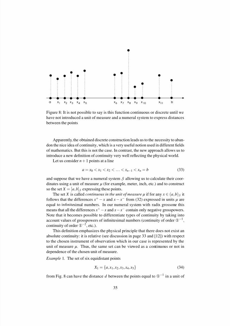
8/3/2019 Yaroslav D. Sergeyev- Blinking Fractals and their Quantitative Analysis Using Infinite and Infinitesimal Numbers
http://slidepdf.com/reader/full/yaroslav-d-sergeyev-blinking-fractals-and-their-quantitative-analysis-using 35/41
Figure 8: It is not possible to say is this function continuous or discrete until wehave not introduced a unit of measure and a numeral system to express distances
between the points
Apparently, the obtained discrete construction leads us to the necessity to aban-
don the nice idea of continuity, which is a very useful notion used in different fields
of mathematics. But this is not the case. In contrast, the new approach allows us to
introduce a new definition of continuity very well reflecting the physical world.
Let us consider n + 1 points at a line
a = x0 < x1 < x2 < ... < xn−1 < xn = b (33)
and suppose that we have a numeral system S allowing us to calculate their coor-
dinates using a unit of measure µ (for example, meter, inch, etc.) and to construct
so the set X = [a, b]S expressing these points.
The set X is called continuous in the unit of measure µ if for any x ∈ (a, b)S it
follows that the differences x+− x and x− x− from (32) expressed in units µ are
equal to infinitesimal numbers. In our numeral system with radix grossone this
means that all the differences x+− x and x− x− contain only negative grosspowers.
Note that it becomes possible to differentiate types of continuity by taking into
account values of grosspowers of infinitesimal numbers (continuity of order x−1,continuity of order x−2, etc.).
This definition emphasizes the physical principle that there does not exist an
absolute continuity: it is relative (see discussion in page 33 and [12]) with respect
to the chosen instrument of observation which in our case is represented by the
unit of measure µ. Thus, the same set can be viewed as a continuous or not in
dependence of the chosen unit of measure.
Example 1. The set of six equidistant points
X 1 = a, x1, x2, x3, x4, x5 (34)
from Fig. 8 can have the distance d between the points equal to x−1 in a unit of
35
8/3/2019 Yaroslav D. Sergeyev- Blinking Fractals and their Quantitative Analysis Using Infinite and Infinitesimal Numbers
http://slidepdf.com/reader/full/yaroslav-d-sergeyev-blinking-fractals-and-their-quantitative-analysis-using 36/41
measure µ and to be, therefore, continuous in µ. Usage of a new unit of measure
ν =x−3
µ implies that d =x2
in ν and the set X 1 is not continuous in ν. 2
Note that the introduced definition does not require that all the points from X
are equidistant. For instance, if in Fig. 8 for a unit measure µ the largest over the
set [a, b]S distance x6− x5 is infinitesimal then the whole set is continuous in µ.
The set X is called discrete in the unit of measure µ if for all points x ∈ (a, b)S
it follows that the differences x+− x and x− x− from (32) expressed in units µ are
not infinitesimal numbers. In our numeral system with radix grossone this means
that in all the differences x+− x and x− x− negative grosspowers cannot be the
largest ones. For instance, the set X 1 from (34) is discrete in the unit of measure ν
from Example 1. Of course, it is also possible to consider intermediate cases where
sets have continuous and discrete parts (see again discussion in page 33 related to
beams from Figs. 6 and 7).
The introduced notions allow us to give the following very simple definition
of a function continuous at a point. A function f ( x) defined over a set [a, b]S
continuous in a unit of measure µ is called continuous in the unit of measure µ at a
point x∈ (a, b)S if both differences f ( x)− f ( x+) and f ( x)− f ( x−) are infinitesimal
numbers in µ, where x+ and x− are from (32). For the continuity at points a, b it
is sufficient that one of these differences is infinitesimal. The notions of continuity
from the left and from the right in a unit of measure µ at a point are introduced
naturally. Similarly, the notions of a function discrete, discrete from the right, and
discrete from the left can be defined.
The function f ( x) is continuous in the unit of measure µ over the set [a, b]S if it
is continuous in µ at all points of [a, b]S . Again, it becomes possible to differentiate
types of continuity by taking into account values of grosspowers of infinitesimal
numbers (continuity of order x−1, continuity of order x−2, etc.) and to consider
functions in such units of measure that they become continuous or discrete over
certain subintervals of [a, b]. In the further consideration we shall often fix the unit
of measure µ and write just ‘continuous function’ instead of ‘continuous function in
the unit of measure µ’. Let us give three simple examples illustrating the introduced
definitions.
Example 2. We start by showing that the function f ( x) = x2 is continuous over
the set X 2 defined as the interval [0, 1] where numerals i
x, 0 ≤ i ≤ x, are used to
express its points in units µ. First of all, note that the set X 2 is continuous in µbecause its points are equidistant with the distance d = x−1. Since this function
is strictly increasing, to show its continuity it is sufficient to check the difference
f ( x)− f ( x−) at the point x = 1. In this case, x− = 1−x−1 and we have
f (1)− f (1−x−1) = 1− (1−x−1)2 = 2x−1(−1)x−2.
This number is infinitesimal, thus f ( x) = x2 is continuous over the set X 2. 2
Example 3. Consider the same function f ( x) = x2 over the set X 3 defined as the
interval [x− 1,x] where numerals x− 1 + i
x, 0 ≤ i ≤ x, are used to express its
36
8/3/2019 Yaroslav D. Sergeyev- Blinking Fractals and their Quantitative Analysis Using Infinite and Infinitesimal Numbers
http://slidepdf.com/reader/full/yaroslav-d-sergeyev-blinking-fractals-and-their-quantitative-analysis-using 37/41
points in units µ. Analogously, the set X 3 is continuous and it is sufficient to check
the difference f ( x)− f ( x−
) at the point x =x to show continuity of f ( x) over thisset. In this case,
x− =x−1 +x−1
x=x−x−1,
f ( x)− f ( x−) = f (x)− f (x−x−1) = x2− (x−x−1)2 = 2x0(−1)x−2.
This number is not infinitesimal because it contains the finite part 2x0 and, as a
consequence, f ( x) = x2 is not continuous over the set X 3. 2
Example 4. Consider f ( x) = x2 defined over the set X 4 being the interval [x−1,x]where numerals x− 1 + i
x2 , 0 ≤ i ≤ x2, are used to express its points in units µ.
The set X 4 is continuous and we check the difference f ( x)
−f ( x−) at the point
x =x. We have
x− =x−1 +x
2−1
x2
=x−x−2,
f ( x)− f ( x−) = f (x)− f (x−x−2) =x2− (x−x−2)2 = 2x−1(−1)x−4.
Since the obtained result is infinitesimal, f ( x) = x2 is continuous over X 4. 2
Let us consider now a function f ( x) defined by formulae over a set X = [a, b]S
so that different expressions can be used over different subintervals of [a, b]. The
term ‘formula’ hereinafter indicates a single expression used to evaluate f ( x).
Example 5. The function g( x) = 2 x2−1, x ∈ [a, b]S , is defined by one formula and
function
f ( x) =
max−10 x, 5 x−1, x ∈ [c, 0)S ∪ (0, d ]S ,4 x, x = 0,
c < 0, d > 0, (35)
is defined by three formulae, f 1( x), f 2( x), and f 3( x) where
f 1( x) =−10 x, x ∈ [c, 0)S , f 2( x) = 4 x, x = 0, f 3( x) = 5 x−1, x ∈ (0, d ]S . 2
(36)
Consider now a function f ( x) defined in a neighborhood of a point x as follows
f (ξ) = f 1(ξ), x− l ≤ ξ < x, f 2(ξ), ξ = x, f 3(ξ), x < ξ≤ x + r ,
(37)
where the number l is any number such that the same formula f 1(ξ) is used to
define f (ξ) at all points ξ such that x− l ≤ ξ < x. Analogously, the number r is
any number such that the same formula f 3(ξ) is used to define f (ξ) at all points ξ
such that x < ξ≤ x + r . Of course, as a particular case it is possible that the same
formula is used to define f (ξ) over the interval [ x− l, x + r ], i.e.,
f (ξ) = f 1(ξ) = f 2(ξ) = f 3(ξ), ξ ∈ [ x− l, x + r ]. (38)
37
8/3/2019 Yaroslav D. Sergeyev- Blinking Fractals and their Quantitative Analysis Using Infinite and Infinitesimal Numbers
http://slidepdf.com/reader/full/yaroslav-d-sergeyev-blinking-fractals-and-their-quantitative-analysis-using 38/41
It is also possible that (38) does not hold but formulae f 1(ξ) and f 3(ξ) are defined
at the point x and are such that at this point they return the same value, i.e.,
f 1( x) = f 2( x) = f 3( x). (39)
If condition (39) holds, we say that function f ( x) has continuous formulae at the
point x. Of course, in the general case, formulae f 1(ξ), f 2(ξ), and f 3(ξ) can be
or cannot be defined out of the respective intervals from (37). In cases where
condition (39) is not satisfied we say that function f ( x) has discontinuous formulae
at the point x. Definitions of functions having formulae which are continuous or
discontinuous from the left and from the right are introduced naturally.
Example 6. Let us study the following function
f ( x) =
x
2 + x2−1 x−1
, x = 1,a, x = 1,
(40)
at the point x = 1. By using designations (37) and the fact that for x = 1 it follows x2−1 x−1
= x + 1 we have
f (ξ) =
f 1(ξ) =x2 +ξ+ 1, ξ < 1, f 2(ξ) = a, ξ = 1, f 3(ξ) =x2 +ξ+ 1, ξ > 1,
Since f 1(1) = f 3(1) =x2 + 2, f 2(1) = a,
we obtain that if a =x2 + 2, then the function (40) has continuous formulae4 at the
point x = 1. Analogously, the function (35) has continuous formulae at the point
x = 0 from the left and discontinuous from the right. 2
Thus, functions having continuous formulae at a point can be continuous or
discrete at this point in dependence of the chosen unit of measure. Analogously,
functions having discontinuous formulae at a point can be continuous or discrete
at this point again in dependence of the chosen unit of measure. The notion of
continuity of a function depends on the chosen unit of measure and numeral sys-
temS
and it can be used for functions defined by formulae, computer procedures,tables, etc. In contrast, the notion of a function having continuous formulae works
only for functions defined by formulae and does not depend on units of measure
or numeral systems chosen to express its domain. It is related only to properties of
formulae.
4Note, that even if a=x2+2+ ε, where ε is an infinitesimal number (remind that all infinitesi-
mals are not equal to zero), we are able to establish that the function has discontinuous formulae.
38
8/3/2019 Yaroslav D. Sergeyev- Blinking Fractals and their Quantitative Analysis Using Infinite and Infinitesimal Numbers
http://slidepdf.com/reader/full/yaroslav-d-sergeyev-blinking-fractals-and-their-quantitative-analysis-using 39/41
8 Conclusion
In this paper, a new type of objects – blinking fractals – that are not covered by
traditional theories studying self-similarity processes have been introduced. They
have been studied together with traditional fractals using infinite and infinitesimal
numbers proposed recently. It has been shown that notions of length, area, and vol-
ume can be extended to the newly introduced and traditional fractals using these
new powerful mathematical tools allowing one to study sets obtained after execu-
tion of different infinite numbers of steps and from different starting conditions. It
has been shown that the new approach allows one to give quantitative characteris-
tics of fractals behavior at infinity.
It has been emphasized that the philosophical triad – researcher, object of in-
vestigation, and tools used to observe the object – existing in such natural sciencesas physics and chemistry exists in mathematics, too. In natural sciences, the in-
strument used to observe the object influences results of observations. The same
happens in mathematics studying numbers and objects that can be constructed by
using numbers. Thus, numeral systems used to express numbers are instruments of
observations used by mathematicians. Usage of powerful numeral systems gives a
possibility to obtain more precise results in mathematics in the same way as usage
of a good microscope gives a possibility to obtain more precise results in physics.
It has been shown in the paper that the new numeral system allowing us to ex-
press not only finite but also infinite and infinitesimal numbers gives a lot of new (in
comparison with traditional numeral systems able to express only finite numbers)
information about behavior of fractal objects at infinity and can be successfullyapplied for numerical analysis of traditional and blinking fractals. Continuing the
analogy with physics we can say that the new numeral system can be compared
with a telescope that allows one to see objects situated infinitely far from the ob-
server and in the same time this telescope has a microscope incorporated that gives
possibility to see infinitesimal parts of this infinitely far objects.
Moreover, the introduced infinite and infinitesimal numbers have allowed us to
propose a new viewpoint on modelling physical continuity in mathematics. The
new approach is closer to the physical world than traditional mathematical instru-
ments used for this purpose and gives a possibility to avoid the existing in the
traditional mathematics contraposition between the notions discrete and continu-
ous. It allows us to look at the same object as at a continuous or a discrete independence of the instrument that is used for observation in the same way as it
happens in physics.
References
[1] V. Benci and M. Di Nasso, Numerosities of labeled sets: a new way of count-
ing, Advances in Mathematics 173 (2003), 50–67.
39
8/3/2019 Yaroslav D. Sergeyev- Blinking Fractals and their Quantitative Analysis Using Infinite and Infinitesimal Numbers
http://slidepdf.com/reader/full/yaroslav-d-sergeyev-blinking-fractals-and-their-quantitative-analysis-using 40/41
[2] G. Cantor, Contributions to the founding of the theory of transfinite numbers,
Dover Publications, New York, 1955.
[3] J.H. Conway and R.K. Guy, The book of numbers, Springer-Verlag, New
York, 1996.
[4] R.L. Devaney, An introduction to chaotic dynamical systems, Westview Press
Inc., New York, 2003.
[5] M.S. El Naschie, A review of E-infinity theory, Chaos, Solitons & Fractals 19
(2004), 209–236.
[6] , A guide to the mathematics of E-infinity Cantorian spacetime theory,
Chaos, Solitons & Fractals 25 (2005), 955–964.
[7] M.S. El Naschie, O.E. Rossler, and I. Prigogine, Quantum mechanics, diffu-
sion and chaotic fractals, Pergamon, Oxford, 1995.
[8] K. Falconer, Fractal geometry: Mathematical foundations and applications,
John Wiley & Sons, Chichester, 1995.
[9] P. Gordon, Numerical cognition without words: Evidence from Amazonia,
Science 306 (2004), no. 15 October, 496–499.
[10] H.M. Hastings and G. Sugihara, Fractals: A user’s guide for the natural sci-
ences, Oxford University Press, Oxford, 1994.
[11] http://www.theinfinitycomputer.com.
[12] G. Iovane, Cantorian spacetime and Hilbert space: Part I – Foundations,
Chaos, Solitons & Fractals 28 (2006), 857–878.
[13] , Cantorian spacetime and Hilbert space: Part II – Relevant conse-
quences, Chaos, Solitons & Fractals 29 (2006), 1–22.
[14] A.A. Markov Jr. and N.M. Nagorny, Theory of algorithms, second ed.,
FAZIS, Moscow, 1996.
[15] K. Knopp, Theory and application of infinite series, Dover Publications, NewYork, 1990.
[16] D. Knuth, The art of computer programming, third ed., Addison-Wesley,
Reading, Massachusetts, 1997.
[17] P.A. Loeb and M.P.H. Wolff, Nonstandard analysis for the working mathe-
matician, Kluwer Academic Publishers, Dordrecht, 2000.
[18] H.-O. Peitgen, H. Jurgens, and D. Saupe, Chaos and fractals, Springer-
Verlag, New York, 1992.
40
8/3/2019 Yaroslav D. Sergeyev- Blinking Fractals and their Quantitative Analysis Using Infinite and Infinitesimal Numbers
http://slidepdf.com/reader/full/yaroslav-d-sergeyev-blinking-fractals-and-their-quantitative-analysis-using 41/41
[19] A.M. Robert, Nonstandard analysis, Dover Publications, New York, 2003.
[20] A. Robinson, Non-standard analysis, Princeton Univ. Press, Princeton, 1996.
[21] Ya.D. Sergeyev, Computer system for storing infinite, infinitesimal, and finite
quantities and executing arithmetical operations with them, patent applica-
tion, 08.03.04.
[22] , Arithmetic of infinity, Edizioni Orizzonti Meridionali, CS, 2003.
[23] , A few remarks on philosophical foundations of a new applied ap-
proach to Infinity, Scheria 26-27 (2005), 63–72.
[24] , Mathematical foundations of the Infinity Computer (invited plenary
lecture), Proc. of the XXI Autumn Meeting of Polish Information Processing
Society (2005), 1–8.
[25] , Misuriamo l’infinito, Periodico di Matematiche 6(2) (2006), 11–26.
[26] B.G. Sidharth, The new cosmos, Chaos, Solitons & Fractals 18 (2003), 197–
201.
[27] R.G. Strongin and Ya.D. Sergeyev, Global optimization and non-convex con-
straints: Sequential and parallel algorithms, Kluwer Academic Publishers,
Dordrecht, 2000.