Yasuhito Tanaka Microeconomic Foundation for Phillips

ISSN: 2543-6821 (online)

Journal homepage: http://ceej.wne.uw.edu.pl

To cite this article

Tanaka, Y. (2021). Microeconomic Foundation for Phillips Curve with a Three-Period Overlapping Generations Model and Negative Real Balance Effect. Central European Economic Journal, 8(55), 163-175.

DOI: 10.2478/ceej-2021-0010

To link to this article: https://doi.org/10.2478/ceej-2021-0010

Microeconomic Foundation for

Phillips Curve with a Three-Period

Overlapping Generations Model

and Negative Real Balance Effect

Yasuhito Tanaka

Open Access. © 2021 Y. Tanaka, published by Sciendo. This work is licensed under the Creative Commons Attribution-NonCommercial-NoDerivatives 4.0 License.

http://ceej.wne.uw.edu.pl

https://doi.org/10.1515/ceej-2018-0003

Yasuhito Tanaka

Department of Economics, Faculty of Economics, Doshisha University, Kamigyo-ku, Kyoto,

602-8580, Japan, corresponding author: [email protected]

Microeconomic Foundation for Phillips Curve with

a Three-Period Overlapping Generations Model

and Negative Real Balance Effect

Abstract We show a negative relation between the inflation rate and the unemployment rate, that is, the Phillips curve using a three-period overlapping generations (OLG) model with childhood period and pay-as-you-go pension for older generation under monopolistic competition with negative real balance effect. In a three-period OLG model, there may exist a negative real balance effect because consumers have debts and savings. A fall (or rise) in the nominal wage rate induces a fall (or rise) in the price, then by negative real balance effect, the unemployment rate rises (or falls), and we get a negative relation between the inflation rate and the unemployment rate. This conclusion is based on the premise of utility maximisation of consumers and profit maximisation of firms. Therefore, we present a microeconomic foundation for the Phillips curve. We also examine the effects of fiscal policy financed by seigniorage, which is represented by left-ward shift of the Phillips curve.

Keywords

microeconomic foundation | monopolistic competition | negative real balance effect | Phillips curve | a three-period

overlapping generations model

JEL Codes

E12, E24, E31

1 Introduction

Otaki and Tamai (2012) presented a microeconomic foundation of the negative relation between the unemployment rate and the inflation rate, that is, the Phillips Curve (Phillips, 1958) using an overlapping generations (OLG) model under monopolistic competition. They showed that, the lower the unemployment rate in a period (e.g., period t–1), the higher the inflation rate from period t to period t–1. Their logic is as follows. They assumed that the low (or high) unemployment rate in period t–1 increases (or decreases) the labour productivity in period t by learning effect. If the unemployment rate in period t–1 increases, the labour productivity in period t falls. Then, by the behaviour of firms in monopolistic competition, the price of the goods in period t rises given nominal wage rate, and the inflation rate from

period t to period t+1 falls given the (expected) price of the goods in period t+1. Alternatively, a decrease in the unemployment rate in period t–1 increases the labour productivity in period t. Then, the price of the goods falls, and the inflation rate from period t to period t+1 increases given the (expected) price of the goods in period t+1. However, we do not find their conclusion that the low unemployment rate in period t–1 explains the high inflation rate from period t to period t+1 to be satisfactory. A fall in the price in period t means that the inflation rate from period t–1 to period t falls, that is, the low unemployment rate in period t–1 explains the low (not high) inflation rate from period t–1 to period t in their model.

Instead, in this article, we consider the effects of a change in the nominal wage rate with negative real balance effect. We use a three-period (three generations) OLG model with childhood period, younger period and

CEEJ • 8(55) • 2021 • pp. 163-175 • ISSN 2543-6821 • DOI: 10.2478/ceej-2021-0010 165

older period. Also, we consider a pay-as-you-go pension system for the older generation to bring about negative real balance effect of a fall in the nominal wage rate. The negative real balance effect (or negative Pigou effect) means that by falls in the nominal wage rate and the price of the goods the real asset of consumers (difference between net savings and debts multiplied by marginal propensity to consume) decreases. The net savings of consumers is the difference between the consumption of consumers in Period 2 (when they are old) and pay-as-you-go pensions.

We will show the negative relationship between the unemployment rate and the inflation rate in the same period. Our logic is as follows. If the nominal wage rate in a period, for example, period t falls, the price of the goods falls. This means that the inflation rate from period t–1 to period t decreases. By the negative real balance effect, the aggregate demand for the goods and employment decreases and the unemployment rate increases in period t. Alternatively, if the nominal wage rate in period t rises, the price of the goods rises, and the inflation rate from period t–1 to period t increases. By the negative real balance effect, the aggregate demand for the goods and employment increases and the unemployment rate decreases in period t. For details, refer Section 4.

There are various studies on the theoretical basis of the Phillips curve from the neoclassical and new Keynesian standpoint. The representative of neoclassical studies is given (Lucas 1972). The neoclassical Phillips curve based on the rational expectation hypothesis is vertical at the natural unemployment rate, but in the short run, incomplete information leads to a downward sloping Phillips curve as firms increase production and employment without realising that the increase in the price of their goods reflects an increase in the general price level. In the new Keynesian analysis, the sticky nature of prices brought about by multi-year wage contracts (Taylor, 1979, 1980) and the sticky pricing behaviour of firms (Calvo, 1983) brings about a downward Phillips curve. Erceg, Henderson and Levin (1998, 2000) developed a similar analysis with a model that incorporates not only price but also wage stickiness, and Woodford (2003) developed an analysis using a model that incorporates an indexation rule such that pricing is linked to the historical inflation rate.

These works on the Phillips curve presume some market imperfection, and it implies that if there does not exist some price stickiness assumption or imperfect information, the negative correlation

between inflation and unemployment will disappear. This article will show that it is not.

In Section 2, we analyse the behaviours of consumers and firms. In Section 3, we consider the equilibrium of the economy with involuntary unemployment. In Section 4, we show the main results about the negative relation between the unemployment rate and the inflation rate due to a change in the nominal wage rate. We also examine the effects of fiscal policy financed by seigniorage, which is represented as left-ward shift of the Phillips curve.

2 Behaviours of Consumers and

Firms

We consider a three-period (childhood, young and old) OLG model under monopolistic competition. It is an extension and arrangement of the model (Otaki 2007, 2009, 2011, 2015). There is one factor of production, labour, and there is a continuum of goods indexed by z [ ]0,1z ∈[0,1]. Each good is monopolistically produced by Firm z. Consumers live over three periods: period 0 (childhood period), period 1 (younger period) and period 2 (older period). There are consumers of three generations, childhood, younger and older generations, at the same time. They can supply only one unit of labour when they are young (period 1).

2.1 Consumers

We use the following notations.

( )ic z : consumption of good z in period , 1, 2i i = .

( )ip z : price of good z in period , 1, 2i i = .iX : consumption basket in period , 1, 2i i = .

( )0c z : consumption of good z in period 0. It is constant.

( )0p z : price of good z in period 0. We assume ( )0 1p z = .

It is constant.


'0X : consumption basket in the childhood period of a consumer of the next generation.

β : disutility of labour, 0β > .

W : nominal wage rate.

P: profits of firms that are equally distributed to the younger generation consumers.

L : employment of each firm and the total employment.

fL : population of labour or employment in the full-employment state.

( )y L : labour productivity. ( ) 1y L ≥ .

R : unemployment benefit for an unemployed consumer, 0R X= .

'R : unemployment benefit for an unemployed consumer in the next generation, '0′ =R X .

Q: the tax for unemployment benefit.

f: pay-as-you-go pension for a consumer of the older generation.

fÖ ': pay-as-you-go pension for a consumer of the younger generation when he is retired.

y: the tax for pay-as-you-go pension.

Consumers in period 0 consume the goods by borrowing money from consumers of the previous generation or the government (e.g. scholarship). They must repay the debts when they are young. However, if they are unemployed, they cannot repay the debts. Then, they receive the unemployment benefits, which are covered by taxes on employed younger generation consumers. Thus, employed younger generation consumers must pay the taxes for unemployment benefit as well as they must repay their own debts. R and Q satisfy the following relation.

(1)

In addition, we consider the existence of pay-as-you-go pension for consumers of the older generation. They are also covered by taxes on employed consumers of the younger generation. Q and y satisfy

(2)

Consumptions in period 0 of the consumers are constant, and in period 1, they determine their

consumptions in periods 1 and 2 and their labour supply. d is the definition function. If a consumer is employed, then 1d = ; if he is not employed, then 0d = . The labour productivity is ( )y L . We consider increasing or constant returns to scale technology. Thus, ( )y L is increasing or constant with respect to the employment of a firm L . We define the employment elasticity of the labour productivity as follows:

( )' .ζ =

yy L

L0 1ζ≤ < , and it is constant. Increasing returns to scale means 0ζ > . η is (the inverse of) the degree of differentiation of the goods. In the limit when η → +∞ , the goods are homogeneous. h and ζ satisfy

( )11 1 1ζη

− + <

so that the profits of firms are positive.

The utility of consumers of one generation over three periods is

( ) ( )0 1 2 0 1 2, , , , , , .U X X X u X X Xd β dβ= −

( )0 1 2, ,u X X X is homogeneous of degree one (linearly homogeneous) with respect to 1X and 2X . Note that 0X is constant. The budget constraint is

( )2p z is the expectation of the price of good z in period 2. Note that 0R X= . The Lagrange function is

l is the Lagrange multiplier. The first-order conditions are

(3)


and

(4)

They are rewritten as

(5)

(6)

Let

,

They are price indices of the consumption baskets in periods 1 and 2. By some calculations, we obtain (see Appendix A)

(7)

and

(8)

The indirect utility of consumers is written as follows:

(9)

( )1 2,P Pj is a function which is homogeneous of degree one. The reservation nominal wage rate RW is a solution of the following equation.

From this, we have

The labour supply is indivisible. If RW W> , the total labour supply is fL . If RW W< , it is zero. If RW W= , then employment and unemployment are indifferent for consumers, and there exists no involuntary unemployment even if fL L< .

Indivisibility of labour supply may be due to the fact that there exists minimum standard of living even in the advanced economy (Otaki, 2015).

Let 2

1PP

ρ = . This is the expected inflation rate (plus one). Since ( )1 2,P Pj is homogeneous of degree one, the reservation real wage rate is

If the value of ρ is given, Rω is constant.

Otaki (2007) assumes that the wage rate equals the reservation wage rate in the equilibrium. However, there exists no mechanism to equalise them.

2.2 Firms

Let1 1 1

1 1 2 2 1 2 , 0 1.α αρ

= = < <+ +

P X XP X P X X X

By some calculations, we obtain the demand for good z of a consumer of the younger generation as follows (see Appendix B):


(10)

Similarly, his demand for good z in period 2 is

Let M be the total savings of consumers of the older generation carried over from their period 1. It is written as

W , L and are nominal wage rate, employment and profit in the previous period, respectively.

, and are the unemployment benefit, tax for the unemployment benefit and tax for the pay-as-you-go pension in the previous period, respectively. Note that F is the pay-as-you-go pension for a consumer of the older generation. M is the total savings or the total consumption of the older generation consumers including the pay-as-you-go pensions they receive in their period 2. It is the planned consumption that is determined in period 1 of the older generation consumers. Net savings is the difference between M and the pay-as-you-go pensions in their period 2, which is written as follows:

With this M, their demand for good z is

( )1

1 1 .p zM

P P

η−

The government expenditure constitutes the national income as well as consumptions of younger and older generations. The total demand for good z is written as

( ) ( )1

1 1 .p zYc z

P P

η−

=

Y is the effective demand defined by

G is the government expenditure other than the pay-as-you-go pensions and the unemployment benefits, and R' R is the consumption in the childhood period of consumers of the next generation (about this demand function, see Otaki (2007, 2009)). The total employment, the total profits and the total government expenditure are written as follows:

We have

( )( ) ( )

( )( )

1 1

1 1 11

( ) .c z c zY p zp z P p zP

η

ηη η− −

−

∂= − = −

∂

From ( ) ( )c z Ly L= ,

( ) ( )( )( )1 1

1 .'

c zLp z y L Ly p z

∂∂=

∂ + ∂

The profit of Firm z is

( ) ( ) ( ) ( ) ( )1 .Wz p z c z c zy L

π = −

1P is given for Firm z. Note that the employment elasticity of the labour productivity is

( )' .y

y LL

ζ =

The condition for profit maximisation with respect to ( )1p z is

( ) ( ) ( )( )

( )( ) ( ) ( ) ( )

( )( )

1 11 1

11 ''

0.'

Lyy L Ly c z c zWc z p z W c z p zy L p z y L Ly p z

− + ∂ ∂ + − = + − = ∂ + ∂


( ) ( ) ( )( )

( )( ) ( ) ( ) ( )

( )( )

1 11 1

11 ''

0.'

Lyy L Ly c z c zWc z p z W c z p zy L p z y L Ly p z

− + ∂ ∂ + − = + − = ∂ + ∂

From this, we have

( ) ( )( )( )( )

( ) ( ) ( )1 1

1

1 .' 1

c zW Wp z p zc zy L Ly y Lp z

ζ η= − = +

∂+ +∂

Therefore, we obtain

( )( ) ( )

1 .11 1

Wp zy Lζ

η

=

− +

With increasing returns to scale, since 0ζ > , ( )1p z is lower than that in a case without increasing returns to scale given the value of W.

3 The Market Equilibrium

3.1 The equilibrium with involuntary

unemployment

Since the model is symmetric, the prices of all goods are equal. Then, ( )1 1 .P p z=Hence

(11)( ) ( )1 .

11 1 ζη

=

− +

WPy L

The real wage rate is

( ) ( )111 1 .W y L

Pω ζ

η

= = − +

Since ζ is constant, this is increasing or constant with respect to L.

The nominal aggregate supply of the goods equals

The nominal aggregate demand is

Since they are equal,

From Eqs (1) and (2), we have

,

and

.

Therefore, we get

This means

In real terms

(12)

or

(13)

If we consider the tax T for the government expenditure, Eq. (13) is as follows:


(14)

11 α− is a multiplier. Eqs (13) and (14) mean that the employment L is determined by g+m. It cannot be larger than L

f

. However, it may be strictly smaller than Lf

(L

< Lf

). Then, there exists involuntary umemployment. Since the real wage rate ( ) ( )11 1 y Lω ζ

η

= − +

is increasing or constant with respect to L, and the reservation real wage rate Rω is constant, if Rω ω> there exists no mechanism to reduce the difference between them.

3.2 Negative real balance effect

When the nominal wage rate falls, the price of the goods (price of consumption basket) falls. If the employment changes, the rate of a fall in the nominal wage rate and that of the price may be different in the case of increasing returns to scale. The real values of G, T, F, F, , Ö, Ö , 'G T R′, R

, , Ö, Ö , 'G T R′ will not change even when the price of the goods falls. On the other hand, the nominal values of R and M-L

f

F will not change. Then, whether the aggregate demand increases or decreases when the nominal wage rate and the price of the goods fall depend on whether

is positive or negative. If <0, there is a negative real balance effect (or Pigou effect)1 such that a fall in the nominal wage rate decreases the aggregate demand because by a fall in the nominal wage rate the real asset of consumers (difference between net savings and debts multiplied by marginal propensity to consume) decreases. Alternatively, a rise in the nominal wage rate increases the aggregate demand.

4. Phillips Curve and Fiscal Policy

4. 1 A change in the nominal wage rate

with negative real balance effect

Suppose that the nominal wage rate falls in a period, for example, period t. From Eq. (11), the price of the

1 About the traditional discussion of real balance effects, refer Pigou (1943) and Kalecki (1944).

goods also falls. Let Pt

and Pt-1 be the price of the goods

(price of the consumption basket) in period t and that in period t–1. The inflation rate from period t–1 to t,

1

1t

t

PP−

− , falls given Pt-1. If the negative real balance effect

works, the real aggregate demand decreases. Then, the output and the employment decrease. Therefore, the lower inflation rate is accompanied by employment loss, that is, higher unemployment rate.

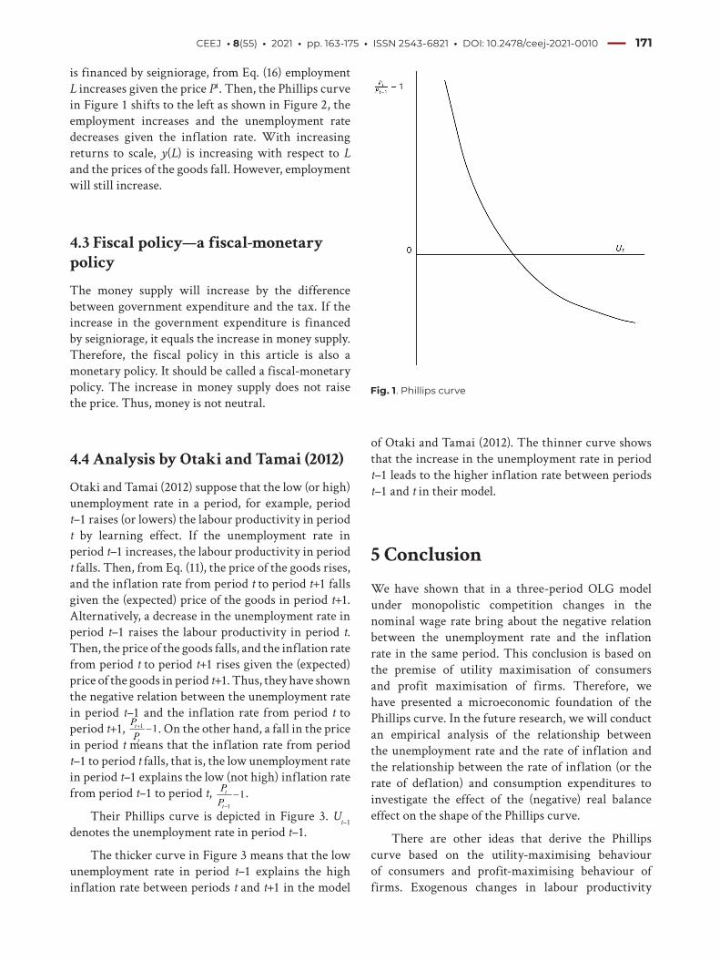
Alternatively, suppose that the nominal wage rate rises. The price of the goods also rises. If the negative real balance effect works, the real aggregate demand increases. Then, the output and the employment increase. Therefore, the higher price or higher inflation rate is accompanied by an increase in employment. Thus, we obtain a negative relationship between the inflation rate and the unemployment rate (positive relationship between the inflation rate and employment) as represented by the Phillips curve. We have shown a negative relationship between the inflation rate and the unemployment rate in the same period given the price in the previous period. Figure 1 depicts an example of the Phillips Curve. U

t

denotes the unemployment rate in period t. Figure 1 implies that our model explains the inflation rate between periods t–1 and t by the unemployment rate in period t.

4.2 Fiscal policy

Let T be the tax revenue other than the taxes for the pay-as-you-go pension system and the unemployment benefits. Then, the budget constraint of the government is G=T, and the aggregate demand is

(15)

With this, the aggregate demand Eq. (14) is

(16)

This implies that the balanced budget multiplier is one.

Given labour productivity y(L) and nominal wage rate W, the price of the goods P1 is determined by Eq. (11). If the government expenditure G increases given T, that is, an increment of the government expenditure


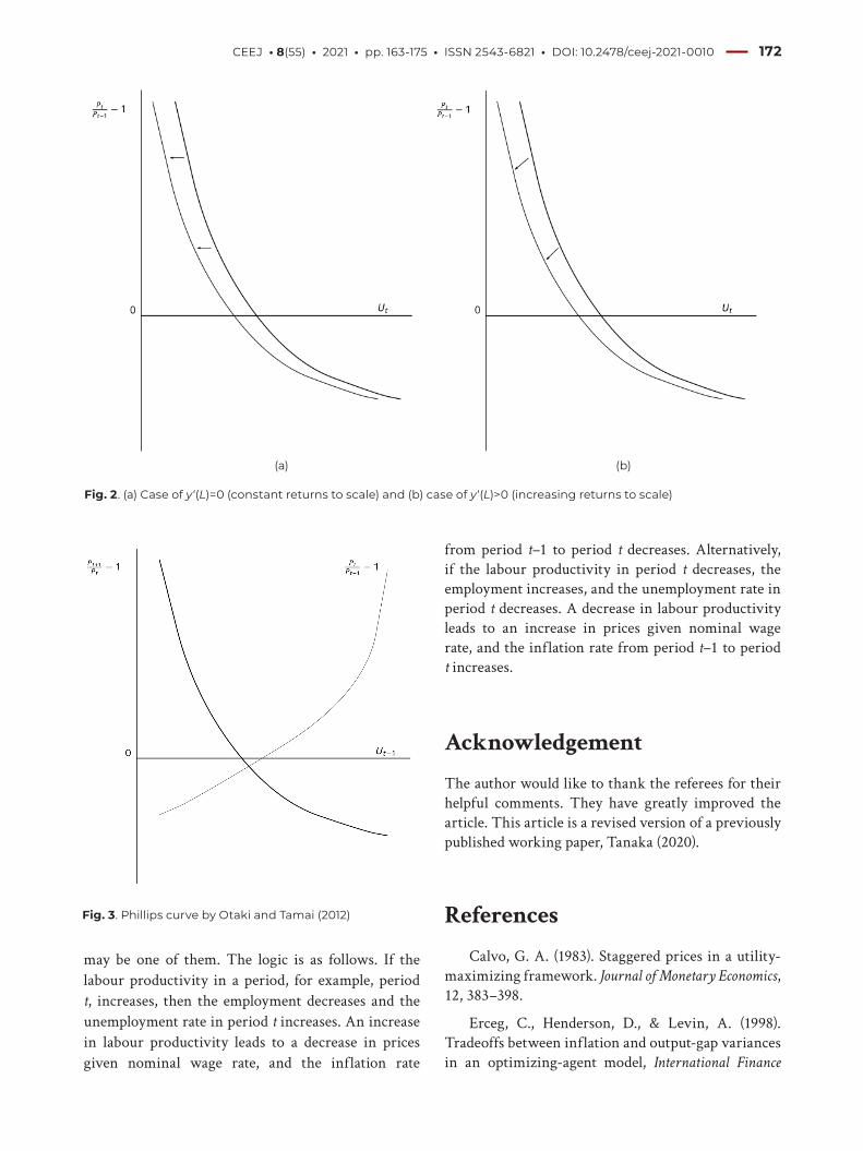
is financed by seigniorage, from Eq. (16) employment L increases given the price P1. Then, the Phillips curve in Figure 1 shifts to the left as shown in Figure 2, the employment increases and the unemployment rate decreases given the inflation rate. With increasing returns to scale, y(L) is increasing with respect to L and the prices of the goods fall. However, employment will still increase.

4.3 Fiscal policy—a fiscal-monetary

policy

The money supply will increase by the difference between government expenditure and the tax. If the increase in the government expenditure is financed by seigniorage, it equals the increase in money supply. Therefore, the fiscal policy in this article is also a monetary policy. It should be called a fiscal-monetary policy. The increase in money supply does not raise the price. Thus, money is not neutral.

4.4 Analysis by Otaki and Tamai (2012)

Otaki and Tamai (2012) suppose that the low (or high) unemployment rate in a period, for example, period t–1 raises (or lowers) the labour productivity in period t by learning effect. If the unemployment rate in period t–1 increases, the labour productivity in period t falls. Then, from Eq. (11), the price of the goods rises, and the inflation rate from period t to period t+1 falls given the (expected) price of the goods in period t+1. Alternatively, a decrease in the unemployment rate in period t–1 raises the labour productivity in period t. Then, the price of the goods falls, and the inflation rate from period t to period t+1 rises given the (expected) price of the goods in period t+1. Thus, they have shown the negative relation between the unemployment rate in period t–1 and the inflation rate from period t to period t+1, 1 1t

t

PP

+ − . On the other hand, a fall in the price in period t means that the inflation rate from period t–1 to period t falls, that is, the low unemployment rate in period t–1 explains the low (not high) inflation rate from period t–1 to period t,

1

1t

t

PP−

− .

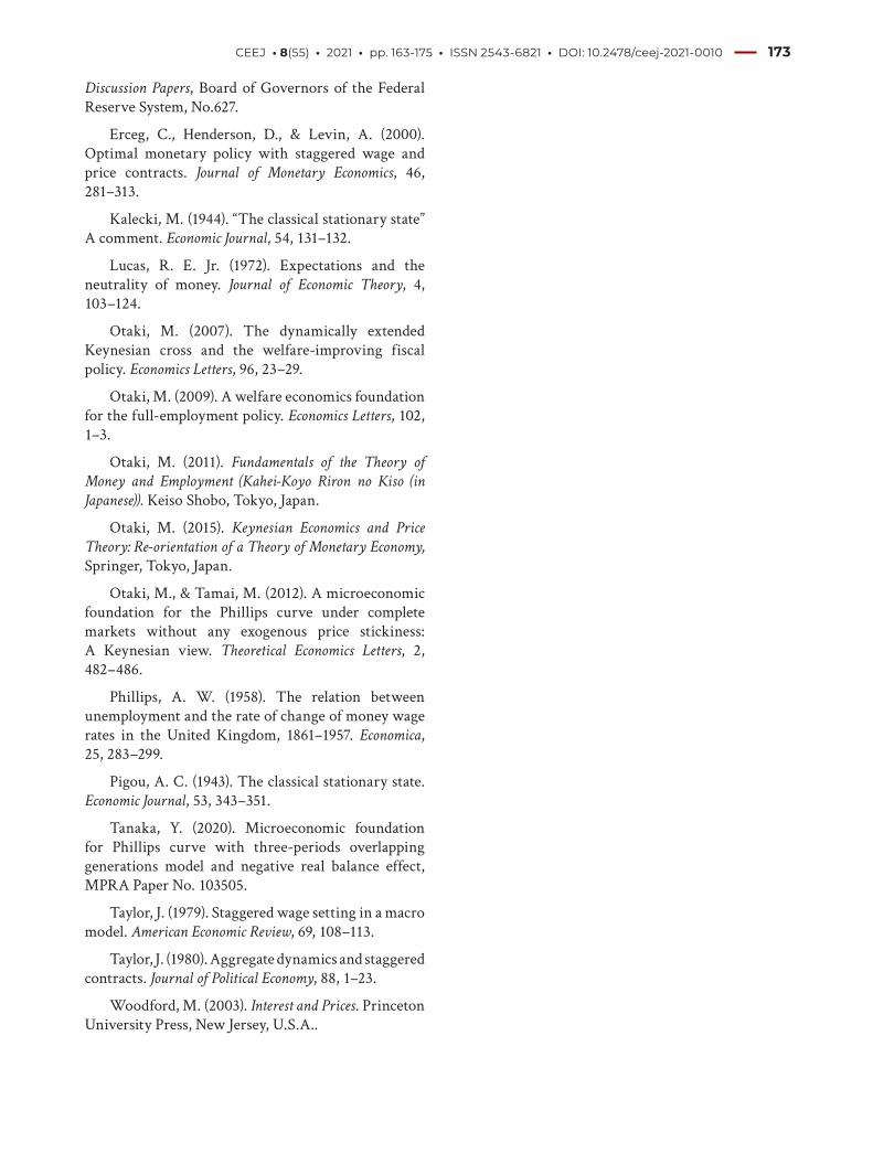
Their Phillips curve is depicted in Figure 3. Ut–1

denotes the unemployment rate in period t–1.

The thicker curve in Figure 3 means that the low unemployment rate in period t–1 explains the high inflation rate between periods t and t+1 in the model

of Otaki and Tamai (2012). The thinner curve shows that the increase in the unemployment rate in period t–1 leads to the higher inflation rate between periods t–1 and t in their model.

5 Conclusion

We have shown that in a three-period OLG model under monopolistic competition changes in the nominal wage rate bring about the negative relation between the unemployment rate and the inflation rate in the same period. This conclusion is based on the premise of utility maximisation of consumers and profit maximisation of firms. Therefore, we have presented a microeconomic foundation of the Phillips curve. In the future research, we will conduct an empirical analysis of the relationship between the unemployment rate and the rate of inflation and the relationship between the rate of inflation (or the rate of deflation) and consumption expenditures to investigate the effect of the (negative) real balance effect on the shape of the Phillips curve.

There are other ideas that derive the Phillips curve based on the utility-maximising behaviour of consumers and profit-maximising behaviour of firms. Exogenous changes in labour productivity

Fig. 1. Phillips curve


may be one of them. The logic is as follows. If the labour productivity in a period, for example, period t, increases, then the employment decreases and the unemployment rate in period t increases. An increase in labour productivity leads to a decrease in prices given nominal wage rate, and the inflation rate

from period t–1 to period t decreases. Alternatively, if the labour productivity in period t decreases, the employment increases, and the unemployment rate in period t decreases. A decrease in labour productivity leads to an increase in prices given nominal wage rate, and the inflation rate from period t–1 to period t increases.

Acknowledgement

The author would like to thank the referees for their helpful comments. They have greatly improved the article. This article is a revised version of a previously published working paper, Tanaka (2020).

References

Calvo, G. A. (1983). Staggered prices in a utility-maximizing framework. Journal of Monetary Economics, 12, 383–398.

Erceg, C., Henderson, D., & Levin, A. (1998). Tradeoffs between inflation and output-gap variances in an optimizing-agent model, International Finance

- 19 -

Figure 2 (a) Figure 2 (b)

Figure 2. (a) Case of ' 0y L (constant returns to scale) and (b) case of

' 0y L (increasing returns to scale).

4.3 Fiscal policy—a fiscal-monetary policy

(a) (b)

Fig. 2. (a) Case of y‘(L)=0 (constant returns to scale) and (b) case of y‘(L)>0 (increasing returns to scale)

Fig. 3. Phillips curve by Otaki and Tamai (2012)


Discussion Papers, Board of Governors of the Federal Reserve System, No.627.

Erceg, C., Henderson, D., & Levin, A. (2000). Optimal monetary policy with staggered wage and price contracts. Journal of Monetary Economics, 46, 281–313.

Kalecki, M. (1944). “The classical stationary state” A comment. Economic Journal, 54, 131–132.

Lucas, R. E. Jr. (1972). Expectations and the neutrality of money. Journal of Economic Theory, 4, 103–124.

Otaki, M. (2007). The dynamically extended Keynesian cross and the welfare-improving fiscal policy. Economics Letters, 96, 23–29.

Otaki, M. (2009). A welfare economics foundation for the full-employment policy. Economics Letters, 102, 1–3.

Otaki, M. (2011). Fundamentals of the Theory of

Money and Employment (Kahei-Koyo Riron no Kiso (in

Japanese)). Keiso Shobo, Tokyo, Japan.

Otaki, M. (2015). Keynesian Economics and Price

Theory: Re-orientation of a Theory of Monetary Economy, Springer, Tokyo, Japan.

Otaki, M., & Tamai, M. (2012). A microeconomic foundation for the Phillips curve under complete markets without any exogenous price stickiness: A Keynesian view. Theoretical Economics Letters, 2, 482–486.

Phillips, A. W. (1958). The relation between unemployment and the rate of change of money wage rates in the United Kingdom, 1861–1957. Economica, 25, 283–299.

Pigou, A. C. (1943). The classical stationary state. Economic Journal, 53, 343–351.

Tanaka, Y. (2020). Microeconomic foundation for Phillips curve with three-periods overlapping generations model and negative real balance effect, MPRA Paper No. 103505.

Taylor, J. (1979). Staggered wage setting in a macro model. American Economic Review, 69, 108–113.

Taylor, J. (1980). Aggregate dynamics and staggered contracts. Journal of Political Economy, 88, 1–23.

Woodford, M. (2003). Interest and Prices. Princeton University Press, New Jersey, U.S.A..


Appendix A: Derivations of Eqs

(7)–(9)

From Eqs. (5) and (6)

Since ( )1 2,u X X is homogeneous of degree one,

Thus, we obtain

and

From Eqs (3) and (4), we have

and

They mean

and

Then, we obtain

and

From them we get

and

Since u(X1, X2) is homogeneous of degree one, l is a function of P1 and P2, and 1

l is homogeneous of degree one because proportional increases in P1 and P2 reduce X

1 and X2 at the same rate given dW+P. We obtain the following indirect utility function.

j(P1, P2) is a function which is homogenous of degree one.


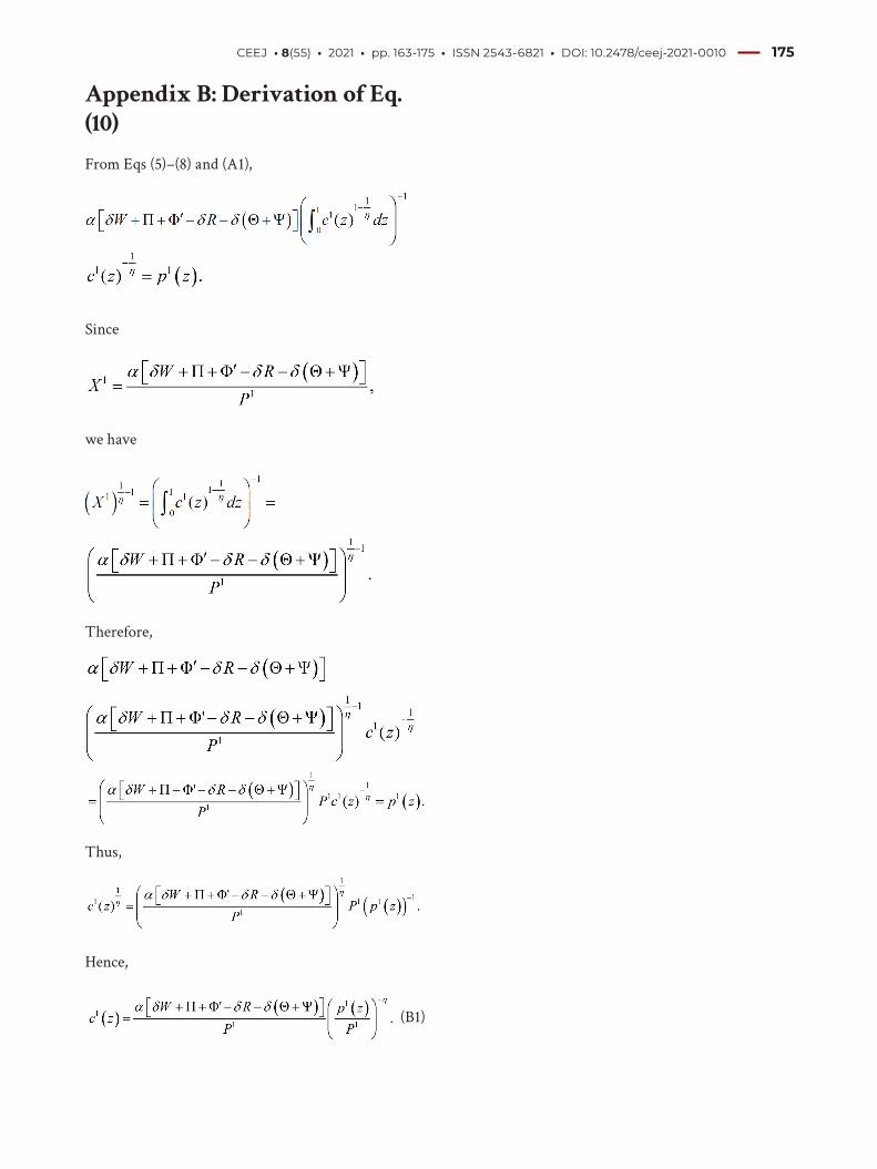
Appendix B: Derivation of Eq.

(10)

From Eqs (5)–(8) and (A1),

Since

we have

Therefore,

Thus,

Hence,

(B1)

Documents

Yasuhito Tanaka Microeconomic Foundation for Phillips