Year 2010 Quasi-Elastic Production at Hadronic Colliders · Quasi-Elastic Production at Hadronic Colliders ... Year 2010 Quasi-Elastic Production ... When trying to nd a solution

Universite de LiegeInteractions Fondamentales en Physique et Astrophysique

Faculte des Sciences

Year 2010

Quasi-Elastic Productionat Hadronic Colliders

Thesis presented in fulfillment ofthe requirements for the Degree of Doctor in Science

Dechambre Alice

Universite de LiegeInteractions Fondamentales en Physique et Astrophysique

Faculte des Sciences

Year 2010

Quasi-Elastic Productionat Hadronic Colliders

Advisor: : J.R Cudell

Member of the jury:

Prof. Joseph CugnonIgor P. Ivanov

Christophe RoyonProf. Jeff Forshaw

President of the jury: Pierre Dauby

Thesis presented in fulfillment ofthe requirements for the Degree of Doctor in Science

15 of July 2010

Abstract: Quasi-elastic production is usually viewed as a golden signal for the de-tection of objects such as the Higgs boson(s) or exotic particles and this is due to the veryclean final state and the lack of hadronic remnants after the interaction. In view of the recentdata from CDF Run II, we critically re-evaluated the standard approach to the calculation ofquasi-elastic cross sections in the high-energy limit and evaluated the uncertainties that affectthis kind of process. The main idea of this work was to understand the various ingredients thatenter the calculation and the uncertainties coming from each of them. We studied and narroweddown these uncertainties using available data on dijets quasi-elastic event at the TeVatron. Allthe arguments developed apply to high-mass central systems and lead to a prediction of theHiggs quasi-elastic cross section at the LHC energies.

Resume: La production quasi-elastique est souvent consideree comme une methodepouvant conduire a d’importantes decouvertes lors de colisions hadron-hadron, en particulierpour la recherche du(des) boson(s) de Higgs ou de particules exotiques. Cela est du a l’absencede pollution hadronique qui rend l’etat final de l’interaction tres simple. En nous basant surles donnees recentes de CDF Run II, nous avons re-evalue de facon critique l’approche standardpour le calcul de la section efficace quasi-elastique dans la limite a haute energie. Les incertitudestheoriques qui affectent ce genre de calcul ont egalement ete etudiees en details. Ce travail aconsiste en l’etude des differents elements qui composent le calcul et a comprendre l’originedes incertitudes provenant de chacun d’entre eux. Nous avons alors pu degager une methoded’analyse qui a permis de les reduire en utilisant les donnees de production quasi-elastiquede dijet au TeVatron. Comme tout les arguments developpes sont identiques quelque soit letype d’objet massif produit, cela nous a permis de donner une estimation de la section efficacequasi-elastique pour la production du boson de Higgs aux energies du LHC.

Acknowledgments:

First of all, I want to thank Jean-Rene. I’m really proud that he was my“third daddy” during my whole PhD-hood, with constant kindness andsupport in my scientific or day-to-day life. Without even noticing, I hadgrown up from the shy student I was to a woman ready to fight for herwork. I have really appreciated his advice and I hope to be able to honourthe knowledge he gave me. I also want to emphasize his courage andabnegation during the corrections to this thesis, especially when dealingwith my mistakes.I particularly thank all the members of the jury and especially Jeff Forshawfor the careful reading of the manuscript and the numerous corrections hemade.

I have also learned a lot from Prof. Joseph Cugnon who first believed thatI could became a particle physicist one day and who has supported meall these years. I thank all the members of the IFPA group including thenumerous visitors. In particular, I thank Igor who started in an impressiveway the work presented in this thesis, Mrs Stancu and Oscar for theirfriendship. A special thank to all the members (permanent or not) of thelunch and coffee breaks on the fourth floor c©, for the useful discussions...or not. Davide, the Local Linux Guru c© and Alex shall inherit my chair,be worth of it. I would also like to add a thought for all people in the B5building and across the world but always behind their computers, Auroreand Angeliki who understand exactly what it means to teach physics tophysicians and other stuff.Not so far from Liege, I would like to thank Christophe Ochando, mypersonal TeVatron advisor and all the people from Saclay. I would also liketo thanks Cyrille who introduced me at the IPhT, I really owe him a roomin that group. He introduced me to Roby and Christophe that showedme a new direction for my work in addition to their trust and kindnesswhen I was trying to walk by myself in the real world. Thank you for thewarm welcome and the 5 o’clock tea. I particularly thank Rafal for all ourdiscussions. When trying to find a solution we were both learning fromour experimental-theoretical points of view.Now I want to thank my family and my parents, my brothers and sisters.Amelie, you are not actually here but I know that you were concerned andfollowed all my steps, you were there each time I needed, even from theend of the earth. Thanks also to Psoman who made the wonderful coverpicture which will add value to my thesis in the future. Meline, you are mysoul mate of studies, as you know what scientific studies mean. Be carefulwith the spiders. You can rely on me all along your way to be a greatbiologist. Clement, because each time I see you I totally forget about allthat scientific stuff. I’m your number one fan! And finally Arthur, “monpetit doudou”, I know that growing up is a long and tough process but Itotally believe in you. You are maybe the only not physicist to have readthe whole thesis, thank you for the corrections and sorry for the sunburn.

My last word is for Vincent. As you were writing your own PhD thesis yousaid that one day we shall stop giving money to Thalys and it is now timeto do so. After long years far away, in which you took care of me regardlessof the distance, now I know what I want.

Contents

Introduction 13

1 Quasi-Elastic Production in High-Energy Physics 151.1 Definitions and Variables . . . . . . . . . . . . . . . . . . . . . . . . . . . . . . . 151.2 Standard Scheme of the Calculation . . . . . . . . . . . . . . . . . . . . . . . . . 171.3 Theory of Quasi-Elastic Processes: A QCD Laboratory . . . . . . . . . . . . . . . 19

1.3.1 The Analytic-S-Matrix Description . . . . . . . . . . . . . . . . . . . . . . 201.3.2 Perturbative QCD Path . . . . . . . . . . . . . . . . . . . . . . . . . . . . 221.3.3 Unsolved Problems in Diffractive QCD . . . . . . . . . . . . . . . . . . . . 22

1.4 Detectors for Quasi-Elastic Events . . . . . . . . . . . . . . . . . . . . . . . . . . 251.4.1 The TeVatron . . . . . . . . . . . . . . . . . . . . . . . . . . . . . . . . . . 251.4.2 The Large Hadron Collider . . . . . . . . . . . . . . . . . . . . . . . . . . 261.4.3 Missing-Mass Measurement . . . . . . . . . . . . . . . . . . . . . . . . . . 30

I Dijet Quasi-Elastic Production 33

2 Perturbative QCD Calculation 372.1 Two-Gluon Amplitude . . . . . . . . . . . . . . . . . . . . . . . . . . . . . . . . . 37

2.1.1 Tools: Contour Integration . . . . . . . . . . . . . . . . . . . . . . . . . . 382.1.2 Toy Calculation . . . . . . . . . . . . . . . . . . . . . . . . . . . . . . . . . 39

2.2 The Longitudinal Integral . . . . . . . . . . . . . . . . . . . . . . . . . . . . . . . 462.3 The Overall Picture . . . . . . . . . . . . . . . . . . . . . . . . . . . . . . . . . . 482.4 Two-Gluon Production . . . . . . . . . . . . . . . . . . . . . . . . . . . . . . . . . 492.5 Gluon Elastic Scattering . . . . . . . . . . . . . . . . . . . . . . . . . . . . . . . . 532.6 The Parton-Level Cross Section . . . . . . . . . . . . . . . . . . . . . . . . . . . . 572.7 Comments . . . . . . . . . . . . . . . . . . . . . . . . . . . . . . . . . . . . . . . . 57

2.7.1 The Second Diagram . . . . . . . . . . . . . . . . . . . . . . . . . . . . . . 59

3 The Impact Factor 633.1 General Properties of Impact Factors . . . . . . . . . . . . . . . . . . . . . . . . . 633.2 Impact Factor from a Quark Model . . . . . . . . . . . . . . . . . . . . . . . . . . 64

3.2.1 Finding the Parameters of the Model . . . . . . . . . . . . . . . . . . . . . 673.3 The Unintegrated Gluon Density . . . . . . . . . . . . . . . . . . . . . . . . . . . 68

3.3.1 Impact Factor from the Unintegrated Gluon Density . . . . . . . . . . . . 713.4 Results and Conclusion . . . . . . . . . . . . . . . . . . . . . . . . . . . . . . . . 73

4 The Sudakov Form Factor 754.1 General Definition of the Resummation . . . . . . . . . . . . . . . . . . . . . . . 754.2 Arbitrariness of the Sudakov Form Factor . . . . . . . . . . . . . . . . . . . . . . 78

4.2.1 Scales . . . . . . . . . . . . . . . . . . . . . . . . . . . . . . . . . . . . . . 78

8 CONTENTS

4.2.2 The Logarithmic Contribution and the Constant Terms . . . . . . . . . . 804.2.3 Sensitivity to the Sudakov Parametrization . . . . . . . . . . . . . . . . . 834.2.4 The Role of the Screening Gluon . . . . . . . . . . . . . . . . . . . . . . . 86

4.3 Summary of the Uncertainties . . . . . . . . . . . . . . . . . . . . . . . . . . . . . 88

5 Additional Soft Corrections 935.1 Gap-Survival Probability . . . . . . . . . . . . . . . . . . . . . . . . . . . . . . . . 93

5.1.1 Definition and Method of Estimation . . . . . . . . . . . . . . . . . . . . . 935.1.2 Beyond the Gap . . . . . . . . . . . . . . . . . . . . . . . . . . . . . . . . 96

5.2 The Splash-Out . . . . . . . . . . . . . . . . . . . . . . . . . . . . . . . . . . . . . 975.2.1 From Partons to Jets . . . . . . . . . . . . . . . . . . . . . . . . . . . . . . 975.2.2 Simple Parametrisation of the Splash-Out . . . . . . . . . . . . . . . . . . 100

6 Results and Conclusion 1056.1 Back-of-the-Envelope Calculation . . . . . . . . . . . . . . . . . . . . . . . . . . . 1056.2 Numerical Implementation . . . . . . . . . . . . . . . . . . . . . . . . . . . . . . . 1086.3 Presentation of the Numerical Results . . . . . . . . . . . . . . . . . . . . . . . . 109

6.3.1 CDF Run II Data . . . . . . . . . . . . . . . . . . . . . . . . . . . . . . . 1106.3.2 Choice of Parametrisation . . . . . . . . . . . . . . . . . . . . . . . . . . . 1116.3.3 Uncertainties . . . . . . . . . . . . . . . . . . . . . . . . . . . . . . . . . . 115

6.4 Extrapolation to the LHC . . . . . . . . . . . . . . . . . . . . . . . . . . . . . . . 1156.5 Conclusion . . . . . . . . . . . . . . . . . . . . . . . . . . . . . . . . . . . . . . . 118

II Higgs Boson Quasi-Elastic Production 119

7 Searching for the Higgs Boson 1257.1 Overview . . . . . . . . . . . . . . . . . . . . . . . . . . . . . . . . . . . . . . . . 125

7.1.1 Higgs-Boson Production in the Standard Model . . . . . . . . . . . . . . . 1257.1.2 The Quasi-Elastic Mode . . . . . . . . . . . . . . . . . . . . . . . . . . . . 127

7.2 The Durham Model . . . . . . . . . . . . . . . . . . . . . . . . . . . . . . . . . . 128

8 Calculation 1318.1 Higgs Boson Production at the Parton Level . . . . . . . . . . . . . . . . . . . . . 131

8.1.1 Higgs Boson Effective Vertex . . . . . . . . . . . . . . . . . . . . . . . . . 1328.1.2 Phase Space . . . . . . . . . . . . . . . . . . . . . . . . . . . . . . . . . . . 134

8.2 Higher-Order Corrections . . . . . . . . . . . . . . . . . . . . . . . . . . . . . . . 136

9 Estimation of the Higgs-Boson Quasi-elastic Cross Section 1399.1 Results . . . . . . . . . . . . . . . . . . . . . . . . . . . . . . . . . . . . . . . . . . 1399.2 Strategy Analysis of Early Data . . . . . . . . . . . . . . . . . . . . . . . . . . . . 1439.3 Summary . . . . . . . . . . . . . . . . . . . . . . . . . . . . . . . . . . . . . . . . 144

A Master Formulae and FORTRAN code 149A.1 Dijet Production . . . . . . . . . . . . . . . . . . . . . . . . . . . . . . . . . . . . 149

B Dijet: Details of the Calculation 153B.1 Integration by Residue . . . . . . . . . . . . . . . . . . . . . . . . . . . . . . . . . 153B.2 Lowest-Order Two-Gluon Production in Quasi-Multi-Regge Kinematics . . . . . 154

B.2.1 s1u2 and u1s2 Diagrams . . . . . . . . . . . . . . . . . . . . . . . . . . . . 154B.2.2 Single-Crossed Diagram u1s2 . . . . . . . . . . . . . . . . . . . . . . . . . 156B.2.3 u1u2 Diagram . . . . . . . . . . . . . . . . . . . . . . . . . . . . . . . . . . 158B.2.4 Comparison of the Two Main Diagrams . . . . . . . . . . . . . . . . . . . 160

CONTENTS 9

B.2.5 The Second Diagram . . . . . . . . . . . . . . . . . . . . . . . . . . . . . . 161B.2.6 Kinematics . . . . . . . . . . . . . . . . . . . . . . . . . . . . . . . . . . . 161B.2.7 Contraction with the First Lipatov Vertex . . . . . . . . . . . . . . . . . . 163

B.3 Sudakov Form Factor . . . . . . . . . . . . . . . . . . . . . . . . . . . . . . . . . 166B.3.1 The DDT Prescription . . . . . . . . . . . . . . . . . . . . . . . . . . . . . 166B.3.2 The Cut-Off Prescription . . . . . . . . . . . . . . . . . . . . . . . . . . . 167B.3.3 The Sudakov Form Factor with Two Scales . . . . . . . . . . . . . . . . . 168B.3.4 Estimation of the Sudakov Suppression . . . . . . . . . . . . . . . . . . . 169

B.4 Model of the Splash-Out: LHE files . . . . . . . . . . . . . . . . . . . . . . . . . . 171B.5 Parametrisation of the Curves . . . . . . . . . . . . . . . . . . . . . . . . . . . . . 172

C Higgs: Details of the Calculation 173C.1 Some Kinematics . . . . . . . . . . . . . . . . . . . . . . . . . . . . . . . . . . . . 173C.2 Contribution of W2 . . . . . . . . . . . . . . . . . . . . . . . . . . . . . . . . . . . 174

So she was considering in her own mind (as well as she could, for thehot day made her fell very sleepy and stupid), whether the pleasureof making a daisy-chain would be worth the trouble of getting up andpicking the daisies, when suddenly a White Rabbit with pink eyes ranclose by her.There was nothing so very remarkable in that; nor did Alice think it sovery much out of the way to hear the Rabbit say to itself, “Oh dear!Oh dear! I shall be too late!” (when she thought it over after-wards, itoccurred to her that she ought to have wondered at this, but at the timeit all seemed quite natural); but when the Rabbit actually took a watchout of its waistcoat-pocket, and looked at it, and then hurried on, Alicestarted to her feet, for it flashed across her mind that she had neverbefore seen a rabbit with either a waistcoat-pocket, or a watch to takeout of it, and burning with curiosity, she ran across the field after it,and fortunately was just in time to see it pop down a large rabbit-holeunder the hedge.In another moment down went Alice after it, never once considering howin the world she was to get out again.

Alice’s Adventures in Wonderland,Lewis Carrol

Introduction

Quasi-elastic production in proton-proton collisions is a process in which the protons do notbreak despite the appearance of a high-mass system. This kind of production has two majorinterests: firstly, the centrally-produced system is within a rapidity gap and clean of hadronicremnants, secondly there is the possibility to measure the energy-momentum lost by the twoinitials protons and to reconstruct the mass of the centrally produced system without detectingit or its decay products. According to these properties, quasi-elastic processes are viewed as a“superb” channel for exotic particle production [1].The first evidence for the existence of this kind of events with the production of a high-masssystem in hadronic collisions was discovered at the TeVatron and published in 2008 by the CDFcollaboration. The data, i.e. the cross section of exclusive dijet production, can be used inorder to compare the different quasi-elastic models on the market and to constrain the differentcalculations. In addition, calculations of various quasi-elastic processes are based on the sameingredients, hence when the parameters are fixed using the dijet data one can use them to makea prediction on other processes, as for instance Higgs boson(s) quasi-elastic production.

This family of processes has small cross sections but their final state is simple and free of hadronicpollution (except from pile-up). This characteristics can be important at the dawn of the LHCera. The energy in the center-of-mass frame of the CERN proton-proton collider should reach14 TeV and will cross 1.15×1011 protons every 25 nanoseconds at its nominal operating condi-tion. This means that a huge number of particles should be produced every 25 nanoseconds andthe four main detectors will have to handle very complex final states. For that reason, even ifthe cross sections of quasi-elastic processes are small, their identification and the identificationof the produced particles is simplified by the possibility to search for gaps in the central detectorand for protons in forward detectors. At the LHC, quasi-elastic processes are competitive andas I write these lines1, the very first proton collision has been observed by the ATLAS andCMS experiments, so that, the hunt is opened.

From the phenomenologist point of view, the calculation of quasi-elastic processes at high-energyis one of the most complete and open topics as it involves many aspects of QCD, from perturba-tive tree-level calculations to non-perturbative corrections. Theoretically, high-energy diffractivecalculations lead to relatively good predictions especially in the domain of hard interactions buttheir richest interest is the possibility to improve and constrain the model using data. Thisduality, to learn from both theory and data, to request theoretical knowledge for the basis anddata for the details or the other way around, always leads to an interesting interplay betweenexperimentalists and theorists as one needs an understanding of the process from the paper tothe detector. Because Nature will always surprise physicists and give them new phenomena toexplain, high energy quasi-elastic calculations are a fascinating playground for phenomenologistsand experimentalists alike.

1November 24, 2009 in the SPP Building at Saclay.

Chapter 1

Quasi-Elastic Production inHigh-Energy Physics

A quasi-elastic process is possible from the exchange of a colour singlet and these quasi-elasticevents are part of a wider class, the diffractive events, which are characterized by a rapiditygap in the final state, between the centrally produced system and the remaining hadrons. Thiswas suggested by Bjorken [1] as a means of detecting new physics in hadron-hadron collisionsbecause of the very simple final state in which rare particles can be produced and decay withoutbackground.

In this chapter, we define quasi-elastic processes and related quantities before explaining theirinterest from both theoretical and experimental points of view. In the second section, we givethe standard scheme of the calculation and each ingredient is introduced before being studied indetails. Because diffractive physics is often synonym of pomeron physics, we briefly introducepresent issues about the pomeron and diffraction in Quantum Chromo-Dynamics (QCD) andfinally, we describe two machines able to study quasi-elastic processes in hadronic collision, theTeVatron and the LHC as well as their dedicated detectors.

1.1 Definitions and Variables

Events with a large rapidity gap between the produced particles and the nucleons in the finalstate have several names. Diffraction is the generic term and the first authors to give a descrip-tion of hadronic diffraction in modern terms were Good and Walker [2] who wrote in 1960:

A phenomenon is predicted in which a high energy particle beam undergoing diffraction scatteringfrom a nucleus will acquire components corresponding to various products of the virtual dissocia-tions of the incident particle [. . . ] These diffraction-produced systems would have a characteristicextremely narrow distribution in transverse momentum and would have the same quantum num-bers of the initial particle.

A hadronic diffractive event is then an elastic event or an event with a rapidity gap but wherethe initial particles break, giving rise to a bunch of final particles which carry the same quan-tum numbers as the initial state. In the present work, we are studying a particular case ofdiffraction with corresponds to the production of particles within a rapidity gap that we shallcall quasi-elastic, considering the fact that it keeps initial hadrons intact as in an elastic colli-sion. In the literature, the same phenomenon is sometimes called exclusive production becauseall final state objects, be they particles or jets, are detected. However, we think that this canbe confusing as the term is used to describe events where all particles in the final state were

16 Quasi-Elastic Production in High-Energy Physics

detected, i.e. centrally produced particles and the remains of the colliding one. In the following,we shall exclusively talk about quasi-elastic production and let us start with a reminder of thevocabulary and pertinent variables.

In a detector, particles can be located using two variables, the azimuthal angle φ and the pseudo-rapidity η defined as

η = − log(

tanθ

2

), (1.1)

where θ is the usual polar angle and so a measurement of θ leads to a measurement of η. Notethat particles or jets with a large pseudo-rapidity are called forward. For high-energy particles,pseudo-rapidity tends to rapidity defined as

y =12

logE + pzE − pz , (1.2)

where E and pz are respectively the energy of the particle and the component of its four-momentum along the z axis. Rapidity is the key variable in diffractive processes because thelarge non-exponentially suppressed rapidity gap in the final state makes it easily recognizablefrom central inelastic hadronic scattering. Indeed, the latter has a flat distribution of particlerapidity due to soft interactions between the two colliding particles as shown in Fig. 1.1. If there

(a) (b)

Figure 1.1: Schematic picture of the rapidity distribution of the products of (a) acentral hadronic scattering and (b) a diffractive hadronic scattering.

is any particle production during the process, the centrally-produced system is within the gap.Actually, there are three different types of event that can give this particular final state, namely:

Quasi-elastic production: Both incoming hadrons emerge intact in the final state,see Fig. 1.2.a.

Single-diffractive production: Only one of the incoming hadrons emerges intact, the secondbreaks but the final system has the same quantum numbers as the initial one, see Fig. 1.2.b.

Double-diffractive production: Both initial hadrons break, see Fig. 1.2.c.

The corresponding rapidity picture of these processes is also drawn in Fig. 1.2. The colouredarea represents the rapidity region where particles can be detected while the white, the lackof hadronic remnants that corresponds to the gap. In diffraction, the final hadrons are brokenbut for quasi-elastic processes, the kinematics is constrained in the region where the energy lostby the initial hadrons, ∆i is small in order to keep them forward. In high-energy physics, thequantity ∆i is one of the essential variables directly related to the fraction of energy lost by

1.2 Standard Scheme of the Calculation 17

∆1

∆2

φ

η

(a)

∆1

∆2

φ

η

X

(b)

∆1

∆2

φ

η

X

Y

(c)

Figure 1.2: The three types of diffractive production and the resulting picture of thefinal state in rapidity in the central detector. The zigzag line denotesthe exchange of a colour singlet and ∆i is the energy lost by the initialhadrons.

the proton (antiproton). If p is the four-momentum of one of the incoming hadrons and ξi thelongitudinal fraction lost by the same hadron then, in the approximation of negligible transferredtransverse momentum, one has

∆i ' ξip, (1.3)

and one can show that the relation between the mass of the centrally produced system and theenergy in the center-of-mass frame of the collision s reads,

M2 ' ξ1ξ2s� s. (1.4)

The advantage of a quasi-elastic process is then a distinctive final state. In addition, this kindof process allows one to reconstruct the mass of the central system from the measurement of thefraction of momentum lost by the initial hadrons. We shall see that this is the event topologythat is really interesting for current detectors and when one has the correct ingredients, thetheoretical calculation of the cross section gives relatively good agreement with available data.

1.2 Standard Scheme of the Calculation

Quasi-elastic processes have been studied from various points of view and within different mod-els [3–16]. The basis of all calculations is the set of tree-level diagrams involving quarks andgluons, upon which one has to add virtual and soft corrections in order to reproduce the fullprocess, from the hadron collision to the final state. The first group who put together most ofthe necessary ingredients was the Durham group [16, 17]. In this thesis, we present a modelmade of five ingredients, related to the Durham scheme, but somewhat different. The variousparts of our model are as follows.

The parton-level calculation: The first ingredient is the analytic computation of all Feyn-man diagrams that describe the production of a colour-singlet and keep the colour ofinitial particles. It is schematically shown in Fig. 1.3.a, the calculation is under theoreticalcontrol. It can be done using cutting rules or direct integration within the kinematicalregime where the momentum lost by the initial particles is small. In particular, we madeefforts to keep an exact transverse kinematics all along the calculation. The lowest-order


cross section is presented in Chapter 2. We discuss there the details of the calculation,the effect of approximations used in [16, 17] and the contribution of diagrams in whichthe screening gluon participates to the hard sub-process, diagrams that were neglected inprevious works.

X

(a)

X

(b)

X

(c)

X

(d) (e)

Figure 1.3: Standard scheme of a quasi-elastic cross section calculation with itsvarious steps.

The impact factor: To describe a collision at the LHC or at the TeVatron, one needs protons(anti-protons) in the initial state. Therefore, the first correction is the introduction ofan impact factor that models the behavior of real protons and embeds the quarks asrepresented in Fig. 1.3.b. The model of the proton includes soft physics and relies on aphenomenological description. Following references [14] and [18], we use theoretical modelsfor the impact factor based on the composition in quarks, light-cone wave-functions, dipoleform factor, ... and tuned to different data (elastic cross section, gluons density, ...).The impact factor is described in Chapter 3 where we consider two ways to embed theperturbative calculation into the proton. The uncertainties coming from the fits will becarefully evaluated.

The Sudakov form factor: One of the most important ingredients of the calculation is theSudakov form factor, i.e. large double-logarithmic terms that suppress the cross section bya factor of the order of 100 to 1000. It corresponds to virtual vertex corrections and in theHiggs case, it is calculated to subleading-log accuracy [19–21]. However, in the dijet casethe single-log contributions have to be evaluated completely and several questions remain.In particular, the dijet vertex cannot be considered point-like at all scales and consequently,we claim that the hard scale of the process is not anymore related to the invariant massof the dijet system. Moreover, we have found that leading and subleading logs that areresummed to give the Sudakov form factor are not dominant for the whole momentumrange, i.e. the constant terms are numerically important. This topic and related issues aredeveloped in Chapter 4.

The gap-survival probability: This is the probability that the gap survives after the firstinteraction. The initial protons that stay intact may re-interact and possibly produceparticles that might fill the gap created at the parton level as schematically shown inFig. 1.3.d. The gap-survival probability is also the probability to have no inelastic inter-actions between the two remaining protons. It is treated as a factor that multiplies thecross section and is discussed in Chapter 5.

The splash-out: The last piece of the calculation is at the very border between theory andexperiment. Before its introduction, one is left with a cross section for partons in thefinal state. To go from partons to real hadrons or jets observed by experimentalists, thereare several steps, i.e. parton showering, hadronization, jet reconstruction algorithms andtagging. This last step is tricky: as there is no perfect matching between the reconstructedjet and the parton that gives birth to it, one can loose some energy from parton to jetand this loss of energy is the splash-out. It is usually treated as a factor and even ifreference [22] considered it, its effect was not really studied in details. In Chapter 5, we

1.3 Theory of Quasi-Elastic Processes: A QCD Laboratory 19

shall show how it is possible to use Pythia and a Monte-Carlo study to approximate theprobability to have a jet of transverse energy Ejet

⊥ from a parton of energy Eparton⊥ .

Each piece of the calculation can be investigated separately, the theoretical approaches developedand the uncertainties evaluated. The phenomenological description of quasi-elastic processes isthus based on the assumption that each ingredient can be studied separately as they matter atdifferent scales, typically two well separated hard and soft scales. The important point is thatsome of the corrections are identical in all quasi-elastic processes so that they can be studied inone particular process then used in another. Consequently, the main idea of the present thesisis to use available data to constrain the different prescriptions for the corrections, i.e. impactfactor, Sudakov form factor, gap survival, splash-out, and this should lead to a more preciseprediction of quasi-elastic cross sections for non-yet observed processes as well as improve ourknowledge in different aspects of QCD. In particular, we focus on the uncertainties and showhow it is possible to use the TeVatron data to reduce some of them. Using that knowledge, weshall extrapolate the model to predict the cross section for dijet and Higgs boson quasi-elasticproduction at the LHC.

The plan of the thesis is then the following. The first part is devoted to the dijet quasi-elasticcross section [23]. All ingredients described above are studied in details and the uncertaintiesthat affect the calculation are evaluated at each step. The second part treats the Higgs bosonquasi-elastic production [24] in the same way and explains how uncertainties are narrowed downusing the dijet study. All results will be presented for both the TeVatron and the LHC.Nevertheless, before coming to the effective calculation, we shall say a few words about the theorybehind quasi-elastic scattering and about the detectors built to study this kind of processes inhigh-energy physics.

1.3 Theory of Quasi-Elastic Processes: A QCD Laboratory

Quasi-elastic processes provide a laboratory where several aspects of QCD can be investigated:soft and hard interactions, exotic particle production, non-perturbative effects or high-energybehavior of the cross section. The present section focuses on the interest from the theoreticalside and we start with the history of diffraction. We continue with two different philosophiesof the theory behind quasi-elastic scattering while the last section is dedicated to some of therelated unsolved problems of QCD.

With the first high-energy hadron accelerators, one needed to describe the dynamics of theproduced events and the observed slow increase of the total cross section with the center-of-mass frame energy [25, 26]. The first success of elastic scattering theory, and consequently ofdiffraction, was to find a mechanism that explained the behavior of the total cross section athigh-energy by the exchange of an object with the quantum numbers of the vacuum called thepomeron [27]. It was the pre-QCD epoch of Regge theory where physicists tried to describestrong interactions within a robust mathematical model of the scattering matrix [28–30]. Theyfocused first on the study of elastic and exclusive processes, i.e. reactions where the kinematicsof the final state is fully reconstructed. Ten years later, the theory of quarks and gluons wasborn [31, 32] and a lot of people chose to turn to inclusive processes where one considers onlytotal rates of production. In the new framework of QCD, the theorem of factorisation [33] al-lows to separate the hard interaction, that produced the leading particles and can be calculatedperturbatively, from the soft ones. Unfortunately no such theorem exists for the diffractive case.In the last two decades, diffractive processes made a come back with the observation of rapiditygap events at HERA [34], followed by the diffraction program of TeVatron. The presence ofthe rapidity gap was then identified by Bjorken [1] as an interesting signature and the interest


in diffraction started slowly to be reborn. It quickly appeared from HERA that this kind ofevents has properties from soft and hard physics at the same time. The idea of hard diffrac-tion was born in 1984 from Donnachie and Landshoff [35] and developed later by Ingelman andSchlein [36], who tried to factorise the soft and hard interactions so that QCD would formulatethe hard collision in terms of quarks and gluons. One would have the possibility from this basisto extend the calculation to the non-perturbative region where soft exchanges occur. It wasrapidly confirmed by the H1 and ZEUS collaboration in 1993 that hard diffraction exists andfew years later, by the UA8 experiment at CERN pp collider [37] but also by the CDF and D0/collaborations at the TeVatron [38]. Unfortunately, it also appeared the the Ingelman-Schleinfactorisation did not work.One can show that colour-singlet exchange between high-energy protons is a very common event,about 25% of the cross section at TeVatron1 is from elastic scattering pp→ pp and another 20%is due to single-diffractive or double-diffractive scattering. Hence, this aspect of QCD is im-portant and will be even more so at the LHC where the center-of-mass frame energy should beequal to

√s = 14 TeV2. This energy will increase the rate of elastic scattering to about 30% of

the total cross section [39] and may allow the production of heavy particles as for example, thewanted Higgs boson(s).

At present, quasi-elastic production is considered as a rich topic of hadronic physics. Thesignature of events is one of the cleanest and the mathematical basis are defined even if importantquestions and issues subsist. We shall now describe the basic concepts of quasi-elastic scatteringfrom two points of view. The first is a description from the analytic-S-matrix theory as softexchanges with an additional hard interaction, the second starts with the hard inclusive processand introduced afterward soft corrections to make it quasi-elastic.

1.3.1 The Analytic-S-Matrix Description

Before the rise of QCD, the first attempt to describe strong interactions relied on the propertiesof the scattering matrix S. In this framework, all scattering processes are described by theirsingularities in the complex-J plane. In the simplest case, these singularities are poles andrepresent the exchange of an infinite number of bound states with the same quantum numbers,except for the spin. The theory predicts the asymptotic behavior of the cross section, i.e. itsbehavior in the limit where the center-of-mass frame energy is much larger than the exchangemomentum |t| and than all masses. Note that is exactly what we requested for quasi-elasticevents in Eq. (1.3).

Without going into much detail, the phenomenological description of scatterings using the an-alytic S-matrix gives the s-channel high-energy behavior of the amplitude due to the exchangeof a family of resonances in the crossed channel. The ensemble of resonances with the samequantum numbers3 lies on a “Regge trajectory” that is a function of t and reads

α(t) = α(0) + α′t. (1.5)

The constant α(0) is called the “intercept” and α′ is the “slope”. There exists different trajecto-ries characterized by the quantum numbers of their resonances and by their slope and intercept.In the S-matrix phenomenology, the amplitude of a given elastic-scattering process is propor-tional to a power of s

1From the Particle Data Group.2Up to now, it appears that due to technical reasons, the LHC should run between

√s = 7 TeV and

√s =

10 TeV.3Parity, charge conjugation, G-parity, isospin, strangeness, etc. apart for their spin.


A ∝ sα(t). (1.6)

Here α(t) is the Regge trajectory corresponding to the quantum numbers of the exchange. Thetotal cross section is related by the optical theorem to

σtot ' 1s

Im (A(0)) ∼ sα(0)−1. (1.7)

At high energy only the highest-spin trajectory contributes and the others are suppressed by apower of s, but if more than one pole are exchanged then the cross section is given by a sumover all contributions

σtot ∝∑Aisαi(0)−1. (1.8)

The values of the slope and the intercept for a given trajectory can be obtained by a fit to totalcross-section data for different processes or center-of-mass frame energies. The important pointis that the S-matrix description leads to a parametrisation of high-energy scatterings for a largeset of data but only in the limit of small momentum transfer. This means that one has here arepresentation of soft exchanges between colliding particles. Note that the exchange of a Reggetrajectory (or reggeon) is usually represented as in Fig. 1.4.a. To explain the growth of the cross

(a) (b)

Figure 1.4: (a) Exchange of a Regge trajectory or reggeon. (b) Inclusion of a hardscattering into the soft exchange. The hard subprocess can be attachedto any of the exchanged pomerons.

section, the pomeron trajectory was introduced, see for instance Sec. 1.3.3. High-energy elasticscattering is thus described by the exchange of a trajectory with the quantum numbers of thevacuum4 and with an intercept of the order of 1. One of the remaining problems is the descrip-tion of multiple pomeron exchanges, this in turn will lead to an uncertainty in the gap-survivalprobability.

In the framework of the analytic scattering matrix, one can see quasi-elastic production asthe embedding of a hard interaction into the above soft exchange schematically pictured inFig. 1.4.b. Two pomerons emitted from the incoming hadrons collide at very short distancesand this collision can be treated separately from the rest of the exchange due to the presenceof a hard scale. The argument is essential and allows to treat separately the hard and the softinteraction, the former can be calculated perturbatively and the latter parametrised, e.g. by itsslope and intercept, using Eq. (1.7) and elastic cross section data. The quasi-elastic productionof any particles is then written in a factorised form

σ = FIP(|t|, s)× σ, (1.9)

where σ is the hard scattering and FIP is either a pomeron flux or a phenomenological softpomeron that includes, in both cases the dependence in s of the cross section. This picture ofpomeron flux is used by the Durham group and in Chap. 7 and can be also found in Chap. 3,

4P=+1, C=+1, I=0.


where we shall use a Regge factor to take into account the dependence of the quasi-elastic crosssection on the center-of-mass frame energy.

1.3.2 Perturbative QCD Path

Quasi-elastic production with gluon fusion can be analysed from the point of view of standardperturbative QCD (pQCD), provided several modifications are made. If one starts with theusual gluon fusion schematically presented in Fig. 1.5, quasi-elastic production can be obtained

Figure 1.5: Production by gluon fusion.

by the addition of a gluon in the t-channel in order to have a colour-singlet exchange.

What seems easy at first sight is not in fact. The hard subprocess producing the final particleis identical in both inclusive and quasi-elastic cases but, in the inclusive case, the cross sectionis summed over all possible final states. In particular, the additional soft exchanges betweenfinal particles disappear in the sum and the calculation is perturbative. Furthermore, at thecross-section level the proton structure functions are well defined in the framework of QCD andcan be measured in different experiments. Three decades of data taking over several ranges ofenergy in the center-of-mass frame and transferred momentum have led to a precise knowledgeof these quantities.In the quasi-elastic case, the addition of the soft screening gluon that prevents colour flow inthe t-channel and the exclusivity of the event definitively change the picture. The factorisationtheorem doesn’t hold and the proton structure functions, that needs to be defined here for verysmall transferred momenta, cannot be used anymore. Furthermore, as the final state is nowspecified, all soft interactions between the different particles of the system should be added.This includes in fact, higher-order and soft corrections in the form of a Sudakov form factor andgap-survival probability, that cannot be fully computed using pQCD and consequently have tobe modeled or fitted to data, bringing in the same time large uncertainties on the final result.

1.3.3 Unsolved Problems in Diffractive QCD

Diffraction and consequently quasi-elastic production seems to have reached a level where oneknows which elements of the cross section are needed to reproduce the data. Moreover, therelatively good agreement between calculations and data suggests that diffraction might bedescribed by the theory of strong interactions [40]. However, diffraction is at the border ofour understanding of QCD and this leads to results affected by large theoretical uncertainties.We stress that the analysis presented here, with the help of recent CDF data, may lead to animprovement in our knowledge of the deep details of quasi-elastic production. Hence, we brieflydiscuss two different issues to give a general idea of the problems one has to deal with whenworking on diffractive physics: the nature of the pomeron and the non-perturbative regimeof QCD.


The Nature of the Pomeron

The pomeron exchange is responsible for the slow rise of the total cross section with s and iscalled after its inventor Pomeranchuk [27]. In the present section, we shall remind the reader ofthe outstanding issues connected with the pomeron IP in QCD.

In the theory of the analytic S-matrix, and as explained in Sec. 1.3.1, a two-body scatteringprocess is described in terms of an exchange of Regge trajectories in the t-channel. The asymp-totic behavior of the total cross section with s is related to the intercept α(0) of the leadingtrajectory by

σtot ∼s→∞

1s

ImA(s, t = 0) ∼s→∞ sα(0)−1. (1.10)

The known mesonic trajectories have intercepts smaller than 1 and thus, their exchange leadsto a decrease of the total cross section with s. Nevertheless, the total cross section increaseswith energy and this unexpected behavior can be explained by the introduction of an additionaltrajectory, dominant at high energy and with a intercept slightly larger than one [29, 30]. Thebound states corresponding to the pole are not related to any known particles but it is usuallyadmitted that they should be bound states of gluons called glueballs5.The parameters, slope and intercept, of the pomeron trajectory can be extracted from a fit toelastic scattering data. This was done by Donnachie and Landshoff in [42] and recently refittedto

αIP(t) = 1.09 + 0.3 t, (1.11)

in the region 0.5 GeV2 < |t| < 0.1 GeV2 and 6 GeV <√s < 63 GeV [43]. It can be argued that

an intercept larger than one would eventually violate the Froissard-Martin bound but multiple-pomeron exchanges should prevent the breakdown of unitarity at higher energy.The difficulty with the pomeron is that, besides an ad-hoc description of the data, its exactnature is not well known considering that QCD is unable to predict the value of the inter-cept. Actually, there exists in the literature two main, but rather different, physical picturesof the pomeron sometimes called the soft and the hard pomeron. The former is a simple butaccurate parametrisation of Regge theory in a large region of data that leads to a small inter-cept αsoft

IP ' 1.1, in the limit of small momentum transfer. The latter derives from the hugeefforts made in the calculation of the exchange of a gluon ladder between two interacting quarksin the framework of pQCD. The pomeron amplitude is then the result of the summation ofleading and subleading log(s) contributions from a number of diagrams and is summarised bythe BFKL equation developed by Balitsky, Fadin, Kuraev and Lipatov [44–47]. The equation in-cludes all transverse momenta, from soft contributions to hard ones, so that all scales are mixed.This hard pomeron is sometimes called the BFKL pomeron and has an intercept of αhard

IP ' 1.5at the leading-log level. Nevertheless, the BFKL approach may reproduce the data only withhuge non-leading corrections [47] and in addition, the calculation is very sensitive to details ofthe IR region where one has to include non-perturbative corrections that complicate the solu-tion [48, 49]. Up to now, the pomeron is just something that makes the cross section increasewith energy and a lot of questions still remain open.

The attempts to describe the nature of the pomeron raise several interesting questions aboutthe scales one is studying in QCD. Experimentalists are left with a huge amount of data fromprocesses that include hard scales and soft scales. Each of the kinematical regimes are describedusing different parametrisation but also different regions of QCD since the soft pomeron is

5Glueballs are expected to be the bound state of at least two gluons, there is now a 2++ candidate and onecan find more details about them in reference [41].


highly non-perturbative whereas the hard one is a perturbative object. It is clearly importantto understand what happens between these two regions and this is why processes at the border,such as hard diffraction and quasi-elastic processes, are still a laboratory where QCD dynamicsat different scales can be studied.

Non-Perturbative Aspects of Diffraction

After the discovery of QCD, the idea of a pomeron pictured as a two-gluon exchange was pro-posed by Low and Nussinov [50, 51] as the simplest way to model a colour-singlet with thequantum numbers of the vacuum. At the Born level, these gluons couple to quarks inside theincoming hadron as shown in Fig. 1.6. Rapidly, it appeared that this simple perturbative picture

Figure 1.6: Elastic scattering via pomeron exchange modeled at the Born levelthrough the exchange of two gluons in the t-channel. The crossed dia-grams are not represented here.

wasn’t sufficient to explain data due to the IR sensitivity of QCD as a non-abelian gauge theorywith confinement. We shall see in Chap. 2 and Chap. 4 that results strongly depend on thedetails of this regime.

Non-perturbative effects naturally appear in the soft corrections to the calculation, i.e. in theimpact factor and in the gap-survival probability. As they cannot be calculated in pQCD, onehas to use instead fits to data or phenomenological models. Hence, those parametrisations areautomatically and irremediably plagued by large uncertainties. One has to allow this intro-duction of non-perturbative effects in the calculation and try to learn as much information aspossible from the data in order to build models and reach a reasonable precision on the crosssection. This is what we shall do for the quasi-elastic case in Chap. 5 and Chap. 6.

Another interesting manifestation of the non-perturbative regime in the calculation is the soft-ness of exchanged gluon momenta. Consequently, if one wants to go beyond the usual per-turbative assumption, the gluon propagator can be modified and this technique is sometimesused to remove the IR divergence of the parton-level amplitude as the IR sensitivity of QCDcomes in part from the gluon propagator itself. One expects the perturbative propagator to bedifferent from the exact propagator of QCD. In particular, one can only trust its shape when thecoupling of QCD becomes small, i.e above twice the mass of the charm quark mc [52]. Purelyperturbative calculations in QCD use the gluon propagator

Dµν(k2) =−igµνδabk2 + iε

, (1.12)

in the Feynman gauge where a and b are colour indices [53]. The IR problem largely comes fromthe pole at k2 = 0 since poles on the real axis correspond to real particles that propagate faraway in space, such a pole is not permitted because gluons are confined. In order to model thenon-perturbative dynamics of QCD that cannot be calculated exactly in the absence of a hard

1.4 Detectors for Quasi-Elastic Events 25

scale, some authors proposed to derive phenomenologically a new gluon propagator. Landshoffand Nachtmann [48] proposed a propagator in the form of a falling exponential

Dµν(k2) = C ek2/Λ2

, (1.13)

that is finite for k2 = 0 and where Λ is a constant related to the scale at which non-perturbativeeffects begin to appear. According to Gribov, it is also possible to improve the quantization ofnon-abelian gauge fields and this leads to a gluon propagator of the form [54],

Dµν(k2) =−igµνδabk2 + Λ4

k2

. (1.14)

The divergence vanishes because the propagator is null at k = 0 and the consequences of theuse of such a propagator in two-gluon exchange was previously studied in [55]. There also existsseveral other possibilities, e.g. adding directly an effective mass µg for the gluon. All these at-tempts to include the contribution of the non-perturbative region into the calculation constitutean important step towards the full description of diffractive processes and more generally ofQCD processes. However, these corrections are tentative at best as if one wants to be complete,the vertices should also be modified and this is even more complicated. The understanding ofthe non-perturbative contributions implies a larger treatment, that is up to now far from ourpresent capabilities.

We shall show that the non-perturbative aspects of the calculation are important and that resultsare sensitive to the details of this regime of QCD but the present knowledge and methods don’tallow to derive those parts reliably, so that one has to use models or fits.

1.4 Detectors for Quasi-Elastic Events

The identification of diffractive events can be done through the particular pattern of the finalstate and is improved by the presence of dedicated forward detectors. In this section, we shallgive a short overview of the present and future detectors able to study details of diffraction atthe TeVatron or the LHC. In the second section, we shall describe the experimental method thatcan be used to reconstruct the mass of the centrally produced system in a quasi-elastic collision.

1.4.1 The TeVatron

The TeVatron is named after the energy −of the order of 1 TeV− of the proton and antiprotonbeams that circulate at the Fermi National Accelerator Laboratory in Illinois. Due to severalsuccessful upgrades since its start in 1983, the energy in the center-of-mass frame is exactly1.960 TeV for the Run II events. The TeVatron has been the highest-energy particle collider inthe world for a long time and its success was the discovery by CDF and D0/, of the top quarksin 1995. Up until now, the TeVatron collaborations are still trying to find the Higgs boson beforethe LHC.

The particularity of the TeVatron is that it collides protons and antiprotons, and as they haveopposite charges, beams travel through the same beam pipe in opposite directions. There aretwo interaction points positioned at opposite sides of the ring as shown in Fig. 1.7. The twodetectors, CDF for Collider Detector at Fermilab [56, 57] and D0/ [58, 59] are built differently, butboth are classical devices for particle physics in which the different sensitive layers are placed in aconcentric way around the beam axis. First a tracker system, then a electromagnetic calorimeter,then an hadronic calorimeter and finally a muon detector. In addition, both CDF and D0/are equipped with forward detectors that extend the rapidity coverage beyond 3.6 and those


detectors can be used to study diffraction during the low-luminosity phases as they principallycollect particles scattered at small angles.

Figure 1.7: Map of the TeVatron. Adapted from [58, 60].

In CDF, which published in 2008 the dijet quasi-elastic cross section measurement, the very for-ward instrumentation is composed of three Roman pot stations located about 57 m downstreamin the antiproton beam direction. Each contains a scintillation counter used for triggering onthe final anti-proton of quasi-elastic or elastic collisions. Note that there is no very forwarddetector on the proton side that hence is not detected.

1.4.2 The Large Hadron Collider

The Large Hadron Collider (LHC) was approved in December 1994 but the construction startedonly at the beginning of 2004 in the old LEP tunnel. Since March 2010, the circulation ofthe beams and the first collisions have been achieved and the data taking started at an energyof√s = 7 TeV. During the recent Workshop on LHC Performance held in Chamonix in Jan-

uary 2010, it was decided to run at this energy until summer or autumn 2011 and by the end ofthe year, one hopes to achieve a luminosity of 3.1 1031 cm−2s−1 [61, 62]. This should be followedby a long shutdown to allow the necessary works to reach the LHC design energy of

√s = 14 TeV.

The LHC has a circumference of 27 km dug at 175 m underneath two countries, France andSwitzerland. Along the tunnel, two beams of protons run in opposite directions inside twobeam pipes and their rotation are controlled by over 1600 superconducting magnets cooled at -271.25 ◦C. This allows engineers to circulate bunches of protons close to the speed of light andwith an energy of several TeV per protons. The nominal commissioned energy of the beamis 7 TeV, leading to collision of 14 TeV in the center-of-mass frame. However, the recent issueswith the supra-conducting magnets have been followed by an early stage of run at 3.5 TeV perbeam that should allow interesting high-energy studies. The two beams can be collided in the


four points of Fig. 1.8, named interaction points (IP), where are built detectors that collect theparticles produced during the interaction.

Figure 1.8: Map of the LHC and its four interaction points with pictures [63–65] oftheir detector: ATLAS (IP1), ALICE (IP2), CMS (IP5) and LHCb (IP8).The top of the remaining octants are occupied by beam maintenance de-vices, beam cleaning and collimation, acceleration cavities and beam dumpsystem [66, 67].


ATLAS and CMS are multi-purpose detectors able to study almost any kind of physics that canpop up. LHCb is dedicated to the study of CP-violation in the production of b-quarks and anti-quarks, looking for an asymmetry in their decays and ALICE is designed to study the physics ofstrongly interacting matter and of the quark-gluon plasma during the heavy-ion collision phase6.From here on, we shall focus on ATLAS and CMS as their design is more adapted to the studyof quasi-elastic events and diffraction.

(a) (b)

Figure 1.9: ATLAS and CMS detectors at the LHC. The two pictures come from theofficial websites [63].

Like most of the detectors, they are constituted by a central inner tracking system, a high resolu-tion electromagnetic calorimeter, a hadronic calorimeter and a muon detector shown in Fig. 1.9.If one includes all the central parts then the rapidity coverage of ATLAS and CMS extendsfrom zero to 3 as shown in Fig. 1.10. The forward calorimeters FCal in ATLAS and the CMS

Figure 1.10: Approximate transverse momentum and rapidity coverage of ATLAS andCMS. Adapted from [68].

hadronic calorimeters HF increase the rapidity range to |η| < 5 and are considered as part of thecentral detector. Particles with higher rapidity are detected in forward detectors, i.e. close tothe beam pipe and far away from the interaction point. Those detectors are on the trajectory of

6The four acronyms stand for A Toroidal Lhc ApparatuS, Compact Muon Solenoid, Large Hadron ColliderBeauty and A Large Ion Collider Experiment.


particles scattered at small angle. Both ATLAS and CMS are completed by Roman pots (RP)designed to measure these particles in the rapidity region of 6.5, their are the T1 and T2 trackersfor CMS and LUCID for ATLAS, measuring the luminosity by counting charge particle tracks7.Both should be used as a trigger for forward detectors TOTEM and ALPHA [69, 70] locatedrespectively at 150 m and 240 m on each sides of the central detector and able to detect protonselastically scattered at angles of the order of 100 µrad. Finally, and this would be the first timeat a hadronic collider, there is a proposal for very forward detectors using Roman Pot techniquesat 220 m and 420 m of the interaction point. They are called respectively RP220 and FP4208.At such distances, they could be hit by protons that have lost a tiny fraction of their initialmomentum and the inclusion of those detectors would make the rapidity coverage reach |η| ∼ 12.

Even without RP220 and FP420, the two multi-purpose detectors of the LHC should be ableto observe diffractive events by triggering on rapidity gaps in the final state. However, it wasshown in the technical reports of the two experiments that a good acceptance and resolution onelastic and quasi-elastic events will be only achieved by the introduction of these very forwarddetectors. In particular, at high luminosity they are useful to reject background.

Forward Detectors

In order to tag the remaining protons of a quasi-elastic scattering event, one has to place adetector close to the beam itself as the protons loose only a tiny part of their momenta andhence stay around their initial bunch. However, it is impossible to put a detector so close to thebeam, as it would be rapidly destroyed by radiation and particle collisions. Thus, one can usethe fact that after about a hundred meters, the final proton is now separated by few millimetersfrom the beam and can hit a strategically placed detector.

The FP420 detector would be located in a small space left on the beam line of LHC and toprotect its sensors during the injection phases it is co-moving with the pipe9. After injectionand when the beam is stable, FP420 can get closer and would be able to collect protons flyingat 10 to 5 mm from the beam. With the addition of these two forward detectors on the rightand on the left of the central detector, CMS is represented in Fig. 1.11 and if one considers the

Figure 1.11: Drawing of the CMS and surrounding detectors at the LHC [71].

addition of both RP220 and FP420, it should be possible to detect protons that have lost a7T1 and T2 stands for Telescope 1 and 2, LUCID means LUminosity measurement using Cerenkov Integrating

Detector.8Recently, they were gathered under the name of ATLAS Forward Physics (AFP) in the ATLAS collaboration

and High Precision Spectrometers (HPS) in the CMS collaboration.9The technique is called the “Hamburg pipe” in reference to a similar setup at HERA.


fraction 0.002 < ξ < 0.2 of their momentum with an acceptance close to 100%. However, theproton tagging has to be related to the central collision. This can be done by measuring thetime of flight from the vertex to the forward detectors. This measurement should also allow thereduction of background by associating the information from both the central and the forwarddetectors. The technique allows a clear identification of quasi-elastic events and seems perfect,apart from the fact that the distance between the central detector and FP420 is too large toadmit any communication, i.e FP420 cannot be used as a Level 1 trigger. Hence, the matchingrequests an exact knowledge of the timing, underlying the importance of high-precision fastdetectors. In particular, the uncertainty on the vertex position is small if the time resolution isgood and it is then possible to match the detection of remaining protons in the right and leftforward detectors with the vertex observed in the central part. If there is no correspondence,the event is rejected as well as most of background events. The time measurement should beachieved by two types of time-of-flight (ToF) detectors, GASTOF and QUARTIC10, that shouldreach a precision of less than 10 ps after a final upgrade [72].

The amazing energy available at the LHC could produce a huge number of particles at eachcollision and the different detectors have to be able to handle that. In the case of quasi-elasticprocesses, pile-up will be a major issue for the analysis but tagging both remaining protonsin addition with the production vertex in the central detector should help to manage some ofit. Moreover, the precise measurement of the momentum of the final protons can be used todetermine the momentum loss and consequently the mass of the system centrally produced.

1.4.3 Missing-Mass Measurement

If the proposal for very forward detectors at both CMS and ATLAS is accepted, the LHC willbe ready to study diffractive physics with a high precision. In particular, a part of the programshould be devoted to quasi-elastic processes for which the unique and clear final state is a realasset.

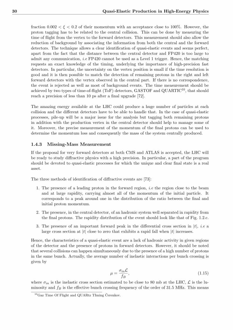
The three methods of identification of diffractive events are [73]:

1. The presence of a leading proton in the forward region, i.e the region close to the beamand at large rapidity, carrying almost all of the momentum of the initial particle. Itcorresponds to a peak around one in the distribution of the ratio between the final andinitial proton momentum.

2. The presence, in the central detector, of an hadronic system well separated in rapidity fromthe final protons. The rapidity distribution of the event should look like that of Fig. 1.2.c.

3. The presence of an important forward peak in the differential cross section in |t|, i.e alarge cross section at |t| close to zero that exhibits a rapid fall when |t| increases.

Hence, the characteristics of a quasi-elastic event are a lack of hadronic activity in given regionsof the detector and the presence of protons in forward detectors. However, it should be notedthat several collisions can happen simultaneously due to the presence of a high number of protonsin the same bunch. Actually, the average number of inelastic interactions per bunch crossing isgiven by

µ =σinLfB

, (1.15)

where σin is the inelastic cross section estimated to be close to 80 mb at the LHC, L is the lu-minosity and fB is the effective bunch crossing frequency of the order of 31.5 MHz. This means

10Gaz Time Of Flight and QUARtz TIming Cerenkov.


that, for a luminosity of 10−34 cm−2s−1, the average number of interactions will be around 25per bunch [67]. All collisions are close in time and space and their final products should beobserved together in the detectors. In particular, some of the products of the additional colli-sions can be detected in the gap region that is then not empty and the event would be rejectedafter triggering. This effect is sometimes called pile-up but the real origin of the name comesfrom the technical effect that is the pileup of several events in the same calorimeter tower. Atthe TeVatron, but also at the LHC, the time between each bunch crossing is smaller that thetime of reaction of the acquisition system and consequently data accumulate in the same partof the detector disturbing the measurement of the energy. In both cases, the result is that thecentrally-produced system or its decay products could be completely hidden in the background,especially at high luminosity.Because of pile-up in the central detector, the mass of the produced system is not easily obtainedbut quasi-elastic production has the interesting feature to allow mass reconstruction from themeasurement of the momentum lost by the initial protons tagged in very forward detectors.

Using the notation of Sec. 1.1 where ξ1, ξ2 are the momentum fractions lost by the protonsand√s the energy in the center-of-mass frame, one indeed has

M2 ∼ ξ1ξ2s, (1.16)

in the approximation of small proton transverse momentum. The uncertainty on mass dependson the precision of the measurement of ξi, itself related to the knowledge of the magnetic field,on the momentum spread of the incoming beams and on the position of the interaction point.According to reference [72, 74], the precision is of the order of 250 MeV at the TeVatron and 2-3 GeV at the LHC, independently of the measured mass. Moreover, the technique allows fora good signal-over-background separation as the resonance peak should appear clearly in themomentum distribution of the final proton. The method is then accurate to measure the massof any object produced in the central region through a quasi-elastic process.

At low luminosity, it should be possible to detect simultaneously the decay products of theparticle(s) and/or the presence of a rapidity gap in addition to the two intact protons in theforward detectors. In this particular case, all particles in the final state are detected and thekinematics fully reconstructed. At high luminosity however, it seems that only the detection offorward protons is relevant and should be used as a filter to measurements in the central detector.This would be possible only if one can deal with the time measurement issues described in theprevious section.

Part I

Dijet Quasi-Elastic Production

The study of dijet quasi-elastic production is particularly interesting in view of the recent datapublished by the CDF RunII collaboration [57] and presented in Fig. 1.12, note that data willbe described in more details in Chap. 6. The cross section is rather small from 1 nb to 1 pb

CDF data

Emin⊥ [GeV]

σ[n

b]

403530252015105

100

10

1

0.1

0.01

0.001

0.0001

Figure 1.12: Cross section of quasi-elastic production of two jets as a function of thejet minimum transverse energy. Data from [57].

depending on the minimum transverse energy of the jet. Nevertheless, it corresponds to 2.105

high-energy dijet events at the TeVatron luminosity11 and one can note that the data includehigh-mass central systems of about 100 GeV. Therefore, the mechanism lies in the kinematicalregion relevant for Higgs boson production for a Higgs boson mass of an hundred GeV and thatcorresponds exactly to the mass range we are interested in, as explained in Chap. 7. In addition,and this is the main point of the present work, data can be used to tune the standard calculationof quasi-elastic cross sections and to narrow down the uncertainties. One can select accurateparametrisations of the soft physics entering the process and use them in other quasi-elasticprocesses taking into account that soft corrections are similar. Thus, one should be able to givea better prediction for dijet and Higgs boson production at the LHC in the quasi-elastic regime.We shall show that the cross section is significant at the LHC, which could provide a large set ofnew data and those data should help reduce even more the uncertainties affecting the calculation.

The aim of this part is to describe in detail the calculation of the cross section for quasi-elasticgluon dijet production. The structure is as follows: first a calculation of the parton-level crosssection (Eq. (2.91) Chap. 2)

Mqq =M(qq → q∗ + gg + q∗), (1.17)

11This number is calculated for a luminosity of 200 fb−1 according to reference [57].

36

followed by the inclusion of the impact factor (Eq. (3.25) Chap. 3)

M(p1p2 → p∗1 + gg + p∗2) =Mqq ⊗ Φ(p1)Φ(p2), (1.18)

of the Sudakov form factor (Eq. (4.1) Chap. 4)

M(p1p2 → p∗1 + gg + p∗2) =Mqq ⊗ Φ(p1)√T (µ2, `21) Φ(p2)

√T (µ2, `22), (1.19)

of the gap-survival probability (Eq. (5.3) Chap. 5)

M(p1p2 → p∗1 + gg + p∗2) =√S2Mqq ⊗ Φ(p1)

√T (µ2, `21) Φ(p2)

√T (µ2, `22), (1.20)

and of the splash-out (Eq. (5.16) and Eq. (5.17) Chap. 5). Each ingredient is studied in dif-ferent chapters and in order to show the uncertainty, each chapter ends on a small discussion.Throughout this study, we select a reference curve shown in Fig. 1.12, coming from a givenmodel that we shall progressively build and given explicitly in Appendix A. We warn the readerthat this curve is not a prediction but rather specific choice that goes through the data. At eachstep of the calculation, i.e. in each chapter detailing a particular piece of the calculation, thiscurve is the reference for a change in the parametrisation of the corresponding ingredients.The last chapter summarises everything, presents the results and discussions, including theprediction for dijet cross section at different LHC energy.

Chapter 2

Lowest Order:Perturbative QCD Calculation

The backbone of the quasi-elastic dijet production is the partonic subprocess

qq → q + gg + q. (2.1)

The central gluon system is in a colour-singlet state and is separated by a large rapidity gapfrom the two scattering quarks. This chapter presents the details of the QCD calculation of theamplitude at the parton level. The first section reminds the reader of integration by residueand other tools that will be used, the second part is the computation of the loop integral and isdivided in two sections. The first one shows how to compute the longitudinal part of the integralbut in a simpler case, the one-particle production for which the kinematics is similar to the dijetcase but less complex. The idea is to identify clearly the different contributions and the structureof the calculation in order to use this knowledge in the two-particle production case. After thatwe focus on the hard subprocess, namely the gluon elastic scattering and present the imaginarypart of the amplitude. The final section is devoted to the study of the theoretical uncertaintieswhere we critically re-evaluate the effect of the usual approximations used in literature.

2.1 Two-Gluon Amplitude

One first has to compute the imaginary part of the diagrams of Fig. 2.1 that is

q − k1

k2 − k3

k1 − k2

q

p p + k3

k

k + k1

k + k3

q + k

p− k

Figure 2.1: Leading diagram for the process qq → q + gg + q. The central blobcorresponds to the gluon-gluon scattering subprocess.

ImM = C g4

∫d4k

(2π4)a(g∗g∗ → gg)

[(q + k)2 + iε][(p− k)2 + iε][(k + k1)2 + iε][(k + k3)2 + iε][k2 + iε](2.2)

38 Perturbative QCD Calculation

where g is the quark-gluon coupling constant and C is the colour factor while a(g∗g∗ → gg)corresponds to the numerator and the amplitude of the hard subprocess.We assume the quarks massless and consider the collision in a frame where the incoming quarkshave no transverse momenta. We introduce the light-cone momenta qµ and pµ that correspondto the direction of the initial quarks with

s = 2 qµpµ, (2.3)

the energy in the center-of-mass frame of the parton-parton collision. The other momenta of theproblem are written using a Sudakov decomposition. The idea is to project the four-momentaupon the incoming particle directions and the transverse plane. In this particular decomposition,

kµ = ypµ + zqµ + kµ,

kµi = yipµ + ziq

µ + kµi ,(2.4)

where transverse vectors are in bold. Note that the notation defined here will be used in thewhole thesis and that

k2 = −kµ kµ,

(k + ki)2 = −(k + ki)µ(k + ki)µ,(2.5)

where the square of transverse momenta are positive quantities. The integration over the four-momentum k is also written in terms of the Sudakov variables,∫

d4k

(2π)4→ s

2(2π)2

∫d2k

(2π)2dydz. (2.6)

The use of the Sudakov parametrisation leads to a clear physical interpretation of variables yi, ziand ki besides a good intuition for what happens during the scattering. One can understand kias the part of the momentum in the perpendicular direction, yi (resp. zi) as the part of the four-momentum in the pµ (resp. qµ) direction and yi � zi indicates that the intermediate particleis more in the direction of the ingoing particle qµ than in the opposite. In addition to theseadvantages, we have the covariance of ki, i.e. a longitudinal Lorentz boost simply changes thefour-vectors pµ and qµ and keeps yi and zi unchanged.

Here we shall keep an exact transverse kinematics, that is to say, the momenta transferred fromthe hadrons, noted ki, are not neglected with respect to the momentum in the loop k.

2.1.1 Tools: Contour Integration

In the calculation of the imaginary part of the amplitude, most integrals in this work are per-formed using contour integration and the Cauchy theorem. Hence, we describe the method.

We would like to compute the integral of f(z) that is an analytic function with a finite numberof poles zi ∫ ∞

−∞f(z)dz. (2.7)

In the calculation of Feynman diagram, these poles come from the propagators. Using theCauchy residue theorem, one can perform the integration along the contour in the complexplane shown in Fig. 2.2 and one obtains

2.1 Two-Gluon Amplitude 39

zi

C∞

z

CR

Figure 2.2: Closed contour C = C∞ + CR in the complex plane and the singularity zi.

∮Cf(z)dz =

∫CRf(z)dz +

∫C∞

f(z)dz

= (2iπ)∑i

Reszi [f(z)],(2.8)

as if f(z) vanishes quickly at infinity, i.e. faster than 1/z, the integration over the half semi-circleis zero and the integral along the z axis is the sum of the pole contributions or residues Reszi [f(z)].Note that when the contour is closed below the z axis, there is an extra-minus sign in front ofthe residue for which the definition depends of the multiplicity of the poles. The residue forsimple poles is

Reszi [f(z)] = limz→zi

(z − zi)f(z), (2.9)

and the formal statement of the Cauchy theorem is given in Appendix. B.1. In the following, weshall make an explicit calculation of the different integrals and it corresponds to the applicationof Cutkosky rules or cutting rules proved by Cutkosky in 1960 [75]. By analogy to them and tocompute the residue, we shall use the prescription to substitute∫

f(z) dz →∫

δ

(1

f(z)

)dz, (2.10)

and the propagator corresponding to the pole zi will be designed as a cut propagator.

Now, we are ready to evaluate the amplitude of the two-gluon quasi-elastic production at theparton level by computing the integral over k and k′ in Eq. (2.2). In particular, one can startby the integral over the longitudinal components of the Sudakov decomposition y and z.

2.1.2 Toy Calculation

We shall first pave the way by computing a similar but simpler case, the production of a masslessparticle as represented with its kinematics in Fig. 2.3.

The momenta transferred from the first and second quarks are k1 and −k3 so that, the four-momentum of the produced particle is

(k1 − k3)µ = αpµ + βqµ + (k1 − k3)µ, (2.11)

with


q − k1 q

p p + k3

k1 − k3

k + k1

k + k3

q + k

p + k + k3

q − k1 q − k1q

p p + k3

k1 − k3k

k + k1

k + k3

q + k

p− k

p + k3

k1 − k3

k + k1

k + k3

p + k + k3

q

p

q − k − k1

k

k

Figure 2.3: Kinematical conventions for the central one-particle production. One hasin turn diagram s1s2, diagram s1u2 and diagram u1u2.

α = y1 − y3,

β = z1 − z3.(2.12)

The central production of a colourless object by pomeron exchange is an example of one-loopparticle production in multi-Regge kinematics and at this order it is known that the amplitudeis dominated by its imaginary part. The leading behavior of the cross section comes from theregion where one has an ordering of the longitudinal momentum fractions [40]

|k2i |s� β, α� 1, (2.13)

while the transverse momenta are of the same order

|k2|, |k21|, |k2

3| � s. (2.14)

The first step is to use the on-shell condition for the produced particle:

(k1 − k3)2 = 0

= αβs− (k1 − k3)2

→ αβs = (k1 − k3)2,(2.15)

and the same for the final quarks

(q − k1)2 = 0

= −y1(1− z1)s− k21

→ y1 =−k2

1

(1− z1)s,

(p+ k3)2 = 0

= z3(1 + y3)s− k23

→ z3 =k2

3

(1 + y3)s.

(2.16)

The last identities also give information about the other longitudinal components consideringthe fact that


y1 − y3 = α → y3 ' −α,z1 − z3 = β → z1 ' β.

(2.17)

The imaginary part of the amplitude can now be evaluated and we first focus on the s1s2 diagram.As the origin of the singularities is in the propagators only, one can first forget about thenumerator and study the integral

∫d4k

(2π)4

1[(q + k)2 + iε][(p− k)2 + iε][(k + k1)2 + iε][(k + k3)2 + iε][k2 + iε]

, (2.18)

where k is the momentum inside the loop. This can be translated to an integral over the Sudakovvariables using Eq. (2.6) and in this section, we are interested in the integral over y and z thatamounts to the evaluation of

Is1s2 =∫

dydz1

[(q + k)2 + iε][(p− k)2 + iε][(k + k1)2 + iε][(k + k3)2 + iε][k2 + iε]. (2.19)

The five propagators are written using Sudakov variables:

P1 = (q + k)2 + iε

= y(1 + z)s− k2 + iε,

P2 = (p− k)2 + iε

= −z(1− y)s− k2 + iε,

P3 = (k + k1)2 + iε

= (y + y1)(z + z1)s− (k + k1)2 + iε,

P4 = (k + k3)2 + iε

= (y + y3)(z + z3)s− (k + k3)2 + iε,

P5 = k2 + iε

= yzs− k2 + iε.

(2.20)

In order to perform the y integral, we first identify the position of the five y poles

yP1 =k2 − iε(1 + z)s

,

yP2 =k2 − iεzs

+ 1,

yP3 =(k + k1)2 − iε

(z + z1)s− y1,

yP4 =(k + k3)2 − iε

(z + z3)s− y3,

yP5 =k2 − iεzs

,

(2.21)

as a function of z and we draw their positions in the upper or in the lower half-plan of the z axisin Fig. 2.4. If one closes the contour below the real axis, there are only three poles that cancontribute simultaneously for specific values of z and as the integrated function quickly vanishes


−1 −z1 −z3 0

−1 −z1 −z3 0

P1

P2

P3

P5

P4

z

z

z

z

z

Figure 2.4: Diagram s1s2: Positions of the y poles of the different propagators asfunctions of z. The shaded regions correspond to poles above the real axiswhile the unshaded ones to poles below the real axis.

at infinity, one can use Eq. (2.10). The longitudinal part of the integral is the sum of the threeresidues

Is1s2 =∫ 0

−1dz∫

dy(−2πi)δ[y(1 + z)s− k2

] 1P2P3P4P5

+∫ 0

−z1dz∫

dy(−2πi)δ[(y + y1)(z + z1)s− (k + k1)2

] 1P1P2P4P5

+∫ 0

−z3dz∫

dy(−2πi)δ[(y + y3)(z + z3)s− (k + k3)2

] 1P1P2P3P5

.

(2.22)

One can directly see that the z variable is always negative so that we change it to −|z| andcalculate separately each of the integrals.

Contribution 1

Let us start with the evaluation of the first term of Eq. (2.22). Using the delta function, one isleft with an integral over z

I1 =∫ 0

−1dz∫

dy(−2πi)δ[y(1− |z|)s− k2

] 1P2P3P4P5

=∫ 0

−1dz∫

dy(−2πi)

(1− |z|)sδ[y − k2

(1− |z|)s]

1P2P3P4P5

=∫ 0

−1dz

(−2πi)(1− |z|)s

1P2P3P4P5

∣∣∣y= k2

(1−|z|)s

.

(2.23)

This second integral is performed using the same technique, we evaluate the position of thez poles for each of the remaining propagator. P5 now gives

k2 = −y|z|s− k2∣∣∣y= k2

(1−|z|)s

= − k2

(1− |z|)s < 0,(2.24)


and is negative-definite due to the kinematics, as well as P3:

(k + k1)2 = (y + y1)(z1 − |z|)s− (k + k1)2∣∣∣y= k2

(1−|z|)s

= − [k(1− β) + k1(1− |z|)]2(1− |z|)(1− β)

< 0,(2.25)

using for the second line the conditions from Eq. (2.16) and Eq. (2.17). Consequently, bothdon’t have poles that can contribute to the imaginary part of the amplitude and one has tocheck only propagators P2 and P4. The former is

(p− k)2 = (1− y)|z|s− k2∣∣∣y= k2

(1−|z|)s

= |z|s− k2

1− |z| ,(2.26)

which changes sign at |z| ' k2/s. The imaginary part of the integral is

Ic11 =∫ 0

−1dz

(−2πi)(1− |z|)2s

(−iπ)s

δ

[|z| − k2

(1− |z|)s]

1P3P4P5

∣∣∣y= k2

(1−|z|)s

= −2π2

s2

1[−k2]

[αk2 − αk2

3 − (k + k3)2]

[−(k + k1)2],

(2.27)

where one has taken the large-s limit and where the index c1 indicates that this is the firstpossible cut. Due to the multi-Regge-kinematics regime, the terms αk2 and αk2

3 are negligiblein front of k2

i , thus the first contribution yields

Ic11 = +2π2

s2

1k2(k + k3)2(k + k1)2

. (2.28)

Putting both propagators P1 and P2 on-shell corresponds to the cut of diagram (a) in Fig. 2.5 andwe shall call it the usual cut contribution. According to [76, 77], the contribution of this cut givesthe imaginary part of the full amplitude and other cut contributions cancel or are negligible.This can be checked by a direct calculation as shown here.Actually, there is also the possibility to use propagator P4. In this case, we substitute y = yP1

and find

(k + k3)2 = (y + y3)(z3 − |z|)s− (k + k3)2∣∣∣y= k2

(1−|z|)s

=(

k2

1− |z| − αs)(

k23

(1− α)s− |z|

)− (k + k3)2,

(2.29)

using again Eq. (2.16) and Eq. (2.17). One can consider two different z regions, namely |z| closeto 1 and |z| ∼ β � 1. In the former case, the propagator P4 becomes

(k + k3)2 ' k2

1− |z| − αs

→ |z| = −k2

αs+ 1,

(2.30)


that is the value at which |z| changes sign and one has to evaluate the integral

Ic21 =−2π2

αs2

1P2P3P5

∣∣∣y= k2

(1−|z|)s ,|z|=−k2

αs+1

' −−2π2

αs2

1[s][−αs][−αs] .

(2.31)

This case leads to a very large y, of the order of α, and to the suppression of the cross sectionby order of s5 due to the other propagators. Thus, the kinematical region of large |z| doesn’tcontribute to the amplitude in the large s-limit. One only has to consider the |z| ∼ β situationfor which propagator P4 simplifies to

(k + k3)2 ' α|z|s− (k + k3)2

→ |z| = (k + k3)2

αs.

(2.32)

The integral yields

Ic31 =∫ 0

−1dz

−2π2

(1− |z|)αs2δ

[|z| − (k + k3)2

αs

]1

P2P3P5

∣∣∣y= k2

(1−|z|)s

' −2π2

s2

1k2(k + k1)2(k + k3)2

.

(2.33)

The contribution corresponds to the cut of diagram (c) of Fig. 2.5 which is actually equal, apartfrom the sign, to the usual contribution of Eq. (2.28).

Contribution 2

The second term of Eq. (2.22) is evaluated in exactly the same way, this time propagator P3 ison-shell and the integral reads

I2 =∫ 0

−z1dz∫

dy(−2πi)

(β − |z|)sδ[y + y1 − (k + k1)2

(β − |z|)s]

1P1P2P4P5

=∫ 0

−z1dz

(−2πi)(β − |z|)s

1P1P2P4P5

∣∣∣y=

(k+k1)2

(β−|z|)s+k2

1(1−β)s

.

(2.34)

Due to kinematics, propagators P1 and P5 cannot be on-shell and one only has to compute thepossible contribution of P2 and P4. We start with P2 and once again, the large |z| region doesn’tcontribute as it is suppressed by a power of s in other propagators. The result is different if oneconsiders the small |z| case for which one has a pole at

(p− k)2 =(

1− (k + k1)2

(z + β)s− k2

1

(1− β)s

)|z|s− k2

' |z|s− k2

→ |z| = k2

s.

(2.35)

Note that due to the assumption of multi-Regge-kinematics |z| = k2/s� α. The evaluation ofthe remaining propagators at the pole leads to


Ic12 =∫ 0

−z1dz

(−2πi)(β − |z|)s

(−iπ)s

δ

[|z| − k2

s

]1

P1P4P5

∣∣∣y=

(k+k1)2

(β−|z|)s+k2

1(1−β)s

' −2π2

βs2

β

[(k + k1)2]1

[−(k + k3)2] [−k2]

' −2π2

s2

1k2(k + k3)2(k + k1)2

.

(2.36)

This cut corresponds to the one shown in Fig. 2.5.b and is, once again, equal and oppositein sign to the usual cut contribution. One is now left with the last piece that comes fromthe pole of propagator P4. The result is straightforward if the produced particle is masslessbecause P4 cannot be put on-shell together with P2 and P3, so that the contribution is zero.This is demonstrated by the negative definiteness of

(k + k3)2 ' −(

(k + k1)2

(β − |z|)s − αs)|z| − (k + k3)2 < 0. (2.37)

Nevertheless, in the case of the production of massive particles such the Higgs boson, the con-tribution of the pole is non-zero and the cut corresponds to the diagram (d) of Fig. 2.5. Onecan estimate the contribution of the pole, starting from Eq. (2.15) that becomes

αβs = (k1 − k3)2 +m2, (2.38)

where m is the mass of the produced particle. Hence,

α =k1 − k3

βs+m2

βs,

β = z1 − z3,

(2.39)

and after a little bit of algebra, one can write the propagator P4 without any approximation as

(k + k3)2 = −1ρ

[(k + k1)(1− ρ) + (k + k3)ρ]2 +m2(1− ρ), (2.40)

with

ρ =z1 + z

z1 − z2. (2.41)

One can show that Eq. (2.40) changes sign at

m2 =[(k + k1)(1− ρ) + (k + k3)ρ]2

ρ(1− ρ), (2.42)

leading to a non-zero contribution to the amplitude. In the general case, i.e arbitrary valueof ki and k, the solution is non-trivial and different from the usual cut contribution. We do notintend to calculate it explicitly, so we simply denote it by

Ic22 =2π2

s2

1k2(k + k1)2(k + k3)2

×∆, (2.43)

where ∆ is a complicated function of ki, k and ρ.


Contribution 3

Finally, we come to the contribution of the third term of Eq. (2.22) that takes into account they pole due to the on-shellness of propagator P4. One has to calculate the integral over z

I3 =∫ 0

−z3dz

(−2πi)(z3 − |z|)s

1P1P2P3P5

∣∣∣y=

(k+k3)2

(z3−|z|)s+α. (2.44)

According to the same argument than in the previous subsection, propagators P2 and P5 cannotbe put on-shell and because P1 and P3 are both positive definite at the pole, this contributionis zero.

Summary

We compile now the results from the different contributions to the s1s2 diagram, the integral isthe sum

Is1s2 = Ic11 + Ic31 + Ic12 + Ic22

=2π2

s2

1k(k + k1)2(k + k3)2

[1− 1− 1 + ∆] ,(2.45)

corresponding respectively to the cuts of Fig. 2.5.

(a) (b) (c) (d)

Figure 2.5: Cuts contributing to the imaginary part of the amplitude. Note thatexcept for the last diagram, all contributions are equal to the usual cutof the first figure apart for the sign. One has respectively Ic11 , Ic31 , Ic12

and Ic22 .

2.2 The Longitudinal Integral

One has now to evaluate the single-crossed and double-crossed diagrams. However, the calcula-tion is left for Appendix B.2 where the reader will find all the details and we compile the resultsobtained from each diagram of Fig. 2.3 to draw the overall picture. In particular, one can notethat contributions are identical apart for the sign and the final answer is

I = Is1s2 + Is1u2 + Iu1s2 + Iu1u2

=2π2

s2

1(k + k1)2(k + k3)2k2

[(1− 1− 1 + ∆) + (1−∆) + (1−∆) + (1 + ∆)]

=2π2

s2

1(k + k1)2(k + k3)2k2

× 2,

(2.46)

that is equal to twice the usual contribution. It is interesting to look at the structure and at thecuts that actually contribute to the imaginary part of the amplitude.

2.2 The Longitudinal Integral 47

s1s2

s1u2

u1s2

u1u2

+1

+1

+1

−1 −1

+1 −∆

−∆

+∆

+∆

Figure 2.6: Non-zero contributions of cuts. The overall sum is equal to twice the usualcut.

From Fig. 2.6, one can directly note that after the sum, contributions that don’t put simulta-neously on-shell the two intermediate quarks cancel with the contribution of the same topologyin the crossed diagram. This can be simply understood if one considers the two diagrams of thesecond column in Fig. 2.6 for which the only difference is the crossing of the bottom line thatleads to the change s2 → u2. Furthermore, one has the identity s2 + u2 + t2 = 0 in the masslesscase, that becomes

s2 ' −u2, (2.47)

in the limit of |t| � s, u and explains the difference of sign. This general structure of thecalculation is analysed in Sec. 2.3 and will be used to compute the longitudinal part of the integralin the two-gluon case. However, the perfect cancellation between some of the contributionscalculated here only takes place if there are no other differences between the three diagrams. Inparticular, there was no colour factor.

Turning the Colour On

If one assumes that the produced particle is colourless and follows the notation of Fig. 2.7, thestructure of the final result of Eq. (2.46), is modified to

C =[(1− 1− 1 + ∆)tatb × tatb + (1−∆)tatb × tbta + (1−∆)tbta × tatb + (1 + ∆)tbta × tbta

]= ∆

[[ta, tb]× [ta, tb]

]+[{ta, tb} × tatb − [ta, tb]× tatb

].

(2.48)


ta tb

ta tb

ta tb

tb ta

ta

ta

tb

tb

Figure 2.7: Indices of the colour factor.

Because we are interested in double pomeron exchange [78], we substitute

tatb → 12N

δab, (2.49)

where N is the number of colours. Subsequently, the cancellation still holds for the contributionproportional to ∆ and one is left with the colour factor

C = {ta, tb} × tatb =1

2N2δabδab =

N2 − 12N2

. (2.50)

Note that if the produced system is in a coloured state, the colour structure is non trivial andthere are no cancellations among the diagrams.

2.3 The Overall Picture

In the previous sections, we have shown that the integral over the longitudinal part of the four-momentum has an imaginary part equal to twice the contribution of the usual cut and thisbecause the others cancel each other. These cancellations between different diagrams can beunderstood in more details.

As explained in Sec. 2.2, one has

si ' −ui, (2.51)

but the effective change of sign can be seen from the fact that going from si to ui only changes thesign of one propagator. As an example, the change in the kinematics when s2 → u2 correspondsto the change of propagator

(q + k)2 → (q − k − k1)2, (2.52)

so that

(1 + z)ys− k2 → −(y + y1)(1− z − z1)s− (k + k1)2. (2.53)

In the case of contributions where only one of the intermediate quarks is on-shell, the ordersof y and z are totally determined by the on-shell condition of the gluon cut. One has

(k + ki)2 = (z + zi)(y + yi)s− (k + ki)2 = 0, (2.54)

for i = 2± 1 using exactly the same kind of notation as in Sec. 2.1. Solving the equation in themulti-Regge-kinematics limit of Eq. (2.13) leads to the conditions

|z| � 1,

y � k2i /s,

(2.55)

2.4 Two-Gluon Production 49

and under those conditions, the change in the propagator simplifies to

ys→ −ys. (2.56)

From these considerations, one finds that the contribution of the s1s2-diagram cancels that ofthe s1u2 diagram, and the same for s1s2 canceling u1s2. This argument also defines the sign ofthe contribution proportional to ∆ and the associated cancellations.

2.4 Two-Gluon Production

The structure of the calculation is exactly the same as in the one-particle production case if oneconsiders a colourless final state. Hereafter, we shall concentrate on the two-gluon productionfor which the kinematics is defined in Fig. 2.8. Let us demonstrate that, in this case too, the

q − k1

k2 − k3

k1 − k2

q

p p + k3

k

k + k1

k + k3

q + k

p− k

k + k2

Figure 2.8: Kinematical conventions in the two-gluon exchange.

amplitude depends only on the usual cut contribution and not on the “wrong” cuts that includeonly one intermediate-quark propagator.

If two gluons are present in the final state, one should take into account all the contributionsof Fig. 2.9 and consider three different situations: the first where only two gluons are attached

Figure 2.9: Diagrams contributing to two-gluon production but cut in the wrong wayor giving a subleading contribution.

to the upper line, the second where an additional gluon is attached outside the loop and the


last where the additional gluon is attached inside the loop. In the former case, the lower partof the diagram remains unchanged from the crossing of the upper line and the only difference isthen the propagator of the upper quark line. As previously, the two diagrams of the first rowof Fig. 2.9 cancel. In the second case, i.e. with an extra gluon attached outside the loop, thevalues assigned to y and z don’t change either and the crossing of the upper quark line onlytransforms the intermediate quark propagator from ys to −ys, leading to cancellations betweenall the diagrams of the second row. At last, one is left with diagrams where one of the finalgluons is emitted from the intermediate quark line. In this particular case, because both quarkpropagators

(q + k)2 = y(1 + z)s− k2 ' ys(q − k1 + k2 + k)2 = (−y1 + y2 + y)(1− z1 − z2 + z)s− (k + k2 − k1)2 ' ys, (2.57)

change sign after the crossing

(q − k − k2)2 = −(y + y2)(1− z2 − z)s− (k + k2)2 ' −ys,(q − k1 − k)2 = −(y1 + y)(1− z1 − z)s− (k + k1)2 ' −ys, (2.58)

there is no cancellation between the usual and the crossed diagrams. Nevertheless, in the regimeof multi-Regge kinematics one has two large additional propagators leading to an extra 1/αsfactor that makes their contribution suppressed at leading order.

The analysis of one- or two-gluon production in multi-Regge kinematics shows that for cen-tral production the contributions of the “wrong” cuts are canceled by the crossed diagrams orare subleading. Besides, the argument can be extended to any similar production in the sameregime, one has only to compute the contributions from the usual cut in order to access theimaginary part of the amplitude. Usual cuts in Fig. 2.9 are suppressed because they lead to aforward jet, which is excluded by kinematical cuts.

Using the previous knowledge, we shall now compute the longitudinal part of the integral for theproduction of two gluons in the central region that constitutes the parton-level calculation forthe production of quasi-elastic dijet. One has to consider the two diagrams of Fig. 2.10 and to

q − k1

k2 − k3

k1 − k2

q

p p + k3

k k + k1

k + k2k + k2 − k3

q − k1

k2 − k3

k1 − k2

q

p p + k3

k

k + k1

k + k3

q + k

p− k

k + k2

Figure 2.10: Contribution to the imaginary part of the amplitude at leading order forthe two-gluon production.

compute the contribution of the cut that puts simultaneously on-shell the intermediate quarks.The momentum transferred from the first and second quarks are k1 and −k3 and we introducethe four-momenta of the two produced gluons,

(k1 − k2)µ = α1pµ + β1q

µ + (k1 − k2)µ,(k2 − k3)µ = α2p

µ + β2qµ + (k2 − k3)µ.

(2.59)

2.4 Two-Gluon Production 51

The amplitude is dominated by its imaginary part and the leading behavior of the cross sectioncomes from the region where one has an ordering of the longitudinal momentum fractions

|k2i |s� β2, β1 � 1,

|k2i |s� α1, α2 � 1, (2.60)

while transverse momenta are of the same order except for k22 that is large

|k2|, |k21| , |k2

3| < |k22| � s. (2.61)

In addition, we work in the high-energy limit s � |t| and in the quasi-elastic regime wherethe longitudinal momentum fractions transferred from the quarks are small to keep the initialparticles intact. In our notation, this means yi, zi � 1.

The first step is to define yi and zi using the on-shell conditions of the final particles

(k1 − k2)2 = α1β1s− (k1 − k2)2 = 0

→ α1β1s = (k1 − k2)2,

(k2 − k3)2 = α2β2s− (k2 − k3)2 = 0

→ α2β2s = (k2 − k3)2.

(2.62)

The same is done for the final quarks

(q − k1)2 = −y1(1− z1)s− k21 = 0

→ y1 =−k2

1

(1− z1)s,

(p+ k3)2 = z3(1 + y3)s− k23 = 0

→ z3 =k2

3

(1 + y3)s.

(2.63)

The last conditions also give information on the other longitudinal component considering thefact that

y2 = y1 − α1 ' −α1,

y3 = y2 − α2 ' −α2,

z1 = z2 + β1 ' β1,

z2 = z3 + β2 ' β2.

(2.64)

We are now ready to evaluate the position of the poles coming from the different propagatorsto compute the integral over the longitudinal part of the first diagram of Fig. 2.10,

I1 =∫

dydz[(q + k)2 + iε][(p− k)2 + iε][(k + k1)2 + iε][(k + k2)2 + iε][(k + k3)2 + iε][k2 + iε]

.

(2.65)Using the Sudakov decomposition of the momenta, the denominators of the propagators become


P1 = (q + k)2 + iε

= y(1 + z)s− k2 + iε,

P2 = (p− k)2 + iε

= −z(1− y)s− k2 + iε,

P3 = (k + k1)2 + iε

= (y + y1)(z + z1)s− (k + k1)2 + iε,

P4 = (k + k2)2 + iε

= (y + y2)(z + z2)s− (k + k2)2 + iε,

P5 = (k + k3)2 + iε

= (y + y3)(z + z3)s− (k + k3)2 + iε,

P6 = k2 + iε

= yzs− k2 + iε,

(2.66)

and according to the preliminary discussion, the only contribution from the cuts is the one thatputs on-shell propagators P1 and P2 in the region where |z| � 1. From the first propagator, onefinds y = k2/(1− |z|)s that is used in P2 to compute the pole in z

P2

∣∣∣y= k2

(1−|z|)s

=(

1− k2

(1− |z|)s)|z|s− k2

' |z|s− k2

→ |z| = k2

s.

(2.67)

Considering both y and z values, one can compute the integral of Eq. (2.65) that is

I1 = −2π2

s2

1k2(k + k1)2(k + k2)2(k + k3)2

. (2.68)

The procedure is repeated to obtain the longitudinal integral of the second diagram of Fig. 2.10and the only difference is from propagators P2 and P5 that become

P2 = (k + k2 − k3)2 + iε

= (y + y2 − y3)(z + z2 − z3)s− (k + k2 − k3)2 + iε

= (y + α2)(z + β2)s− (k + k2 − k3)2 + iε,

P5 = (p− k − k2 + k3)2 + iε

= −(1− y − y2 + y3)(z + z2 − z3)s− (k + k2 − k3)2 + iε

= −(1− y − α2)(z + β2)s− (k + k2 − k3)2 + iε.

(2.69)

using Eq. (2.64). The contributing poles are again those that correspond to the usual cut andput P1 on-shell together with P2. The integration region of |z| is now between β2 and 1 leadingto

I2 = −2π2

s2

1k2(k + k1)2(k + k2)2(k + k2 − k3)2

. (2.70)

2.5 Gluon Elastic Scattering 53

The colour factors are different for the two diagrams and one can compute them using Eq. (2.49)and Fig. 2.11.

a b

c1

c2b′′

a b′

Figure 2.11: Indices of the colour factor.

Therefore, for the first diagram one can show that

C1 =(tatb × tatb′

)f bc1b

′′f b′′c2b′ =

−14N

δc1c2 , (2.71)

that corresponds to the emission of a coloured object at each three-gluon vertices and where Nstands for the number of colour. For the second diagram

C2 =(tatb × ta′tb′

)f bc1b

′fac2a

′=

14N

δc1c2 . (2.72)

The opposite sign of the crossed diagram implies that its contribution decreases the dijet crosssection. Taking into account that it is usually neglected, one can stress that the dijet crosssection is an upper limit to the process.

We have calculated the integral on the longitudinal momentum of the imaginary part of theamplitude for the two gluons to a colour-singlet state. We have shown that the situation simpli-fies due to the fact that several contributions cancel each other and the final result reduces totwo simple expressions that depend only on transverse momenta. Note that the second diagramhas an additional large propagator (k + k2 − k3)2 and because k2

2 is large in front of the othertransverse momenta in the considered kinematics, this leads to the suppression of the seconddiagram with respect to the first1. Consequently, we shall focus on the first diagram only butthe contribution of the second will be studied as a correction in the last chapter. The imaginarypart of the amplitude of Eq. (2.2) becomes

ImM =g4

4π2

δc1c2

4N2

∫d2k

k2(k + k1)2(k + k3)2× a(g∗g∗ → gg). (2.73)

2.5 Gluon Elastic Scattering

The final two-gluon state is produced by the elastic scattering of two gluons of momenta k +k1 and k + k3. The amplitude of the corresponding process a(g∗g∗ → gg) is calculated in theFeynman gauge using the helicity amplitude method.

1This statement is developed in Appendix B.2 where we estimate analytically the two-gluon production inquark-quark scattering and the particular case of quasi-multi-Regge kinematics using standard Lipatov vertices.


We have defined

a(g∗g∗ → gg) =∑λi

j(1)∗λ1

j(2)∗λ2M(g∗λ1

g∗λ2→ gλ3gλ4), (2.74)

where M(g∗g∗ → gg) corresponds to the amplitude of the hard subprocess of Fig 2.12 and thecurrent j will be defined below. If one first considers the amplitude q → qg, one has

q − k1

k2 − k3

k1 − k2

q

p p + k3

k

k + k1

k + k3

q + k

p− k

Figure 2.12: Leading diagram for the process qq → q + gg + q in the high-k22 regime.

The central blob corresponds to the gluon-gluon scattering subprocess.

j(1)λ1

= u(q + k)γ.e∗λ1u(q − k1),

j(2)λ2

= u(p− k)γ.e∗λ2u(p+ k3),

(2.75)

as the imaginary part is calculated for the cut that puts the intermediate quarks propagators q+k and p−k on-shell. Now, we focus on the gluon scattering. Strictly speaking, the two collidinggluons are virtual. However, in our kinematics their off-shellness are equal to −k2

1 and −k23

that are much smaller, in modulus, than the hard scale of the subprocess k22. So, one can

neglect the non-zero virtualities and approximate the amplitude by the scattering of two on-shelltransversely polarized gluons and that corresponds to the sum of the four diagrams of Fig. 2.13.The Mandelstam invariants of the process can be written as a function of the Sudakov variables

= + + +

Figure 2.13: Two-gluon elastic scattering.

of the final gluons and yield

sgg = M2gg ' k2

2

(β1 + β2)2

β1β2, tgg ' −k2

2

β1 + β2

β1, ugg ' −k2

2

β1 + β2

β2. (2.76)

The helicity amplitude for the tree level scattering of two gluons in a colour-singlet state in thecenter-of-mass frame is

M(gλ1gλ2 → gλ3gλ4) = 2g2h

N

N2 − 1δabδc1c2

(sggtgg

+sggugg

)ei(λ1−λ2)φA(λ1λ2 → λ3λ4), (2.77)

2.5 Gluon Elastic Scattering 55

where gh is the strong coupling constant and λi the helicities. The non-zero helicity ampli-tudes A(λ1λ2 → λ3λ4) of the previous equation are

A(++→ ++) = A(−− → −−) = 1,

A(+− → +−) = A(−+→ −+) =u2gg

s2gg

,

A(+− → −+) = A(−+→ +−) =t2ggs2gg

.

(2.78)

Here, we denote by φ the azimuthal angle of the final two-gluon production plane with respectto the quantization axis that is arbitrary, taking into account that a change will be compensatedby an opposite change in the current j(i)

λi. One can align the axis of the gluon collision with

the laboratory frame. This is because to go from the latter to the former, one has to perform alongitudinal boost to make the energy of the colliding gluons equal, a transverse boost to makethe total momentum of the two-gluon system zero, and finally a rotation to align the z axiswith the direction of the incoming gluons. If the longitudinal boost doesn’t change φ, the trans-verse boost and the rotation at small angle have a negligible effect on the hard momentum k2.Therefore, one can safely understand the angle of the final gluons production plane as the az-imuthal angle in the laboratory frame. Their polarisation vectors can be chosen orthogonal toboth k + k1 and k + k3 and, within our accuracy, they can be generically written as

eµλ = eµλ +2s

(pµ

eλ.(k + k1)β1 + β2

+ qµeλ.(k + k3)α1 + α2

), (2.79)

where we use the standard definition of the polarization vector in the transverse plane

eλ = − 1√2

(λ, i). (2.80)

The incoming gluons have λ = λ1 and λ = −λ2 since they move in opposite longitudinaldirections and one can now simplify Eq. (2.75) to

j(1)∗λ1' 2

e∗λ1.(k + k1)β1 + β2

= − 2β1 + β2

λ1√2|k + k1|e−iλ1φ1 ,

j(2)∗λ2' 2

e∗−λ2.(k + k3)

α1 + α2

=2

α1 + α2

λ2√2|k + k3|eiλ2φ3 ,

(2.81)

where φ1 and φ3 are respectively the azimuthal angles of k + k1 and k + k3. To obtain the crosssection, one has to take the square of the amplitude that is∑

f

∑λi,λ′i

j(1)∗λ1

j(2)∗λ2

j(1′)λ′1

j(2′)λ′2Mλ1λ2→fM∗λ′1λ′2→f , (2.82)

if f labels the polarization states of the final gluon system. The only non-trivial interference isbetween M+−→f and M−+→f for both f = +− and f = −+ because such a term introducesan azimuthal dependence for high |k2| via a factor exp(4iφ). It contributes to the azimuthalcorrelations between the plane of the high transverse energy jets and that of the quark scattering.


However, after integration over φ, keeping the cross section differential in k2, this term vanishesand this allows one to consider only the diagonal contribution λ′i = λi. The result is

∑f

∑λi

j(1)∗λ1

j(2)∗λ2

j(1′)λ1

j(2′)λ2|Mλ1λ2→f |2

=∑f

∑λi

8|k + k1||k + k3||k′ + k1||k′ + k3|

(β1 + β2)2(α1 + α2)2

14e−i(λ1φ1−λ2φ3−λ1φ′1+λ2φ′3)A(λ1λ2 → f).

(2.83)

We would like to present the result in a way that will be useful for the discussion of Chap. 6,so that we separate the case where the total helicity of the final gluon system λ = λ1 − λ2 isequal to 0 from the λ = 2 case. We denote the function depending on λi by M and one hasrespectively

|M0|2 =12[|A++→++|2 + |A−−→−−|2

]= 1, (2.84)

|M2|2 =12[|A+−→+−|2 + |A+−→−+|2 + |A−+→−+|2 + |A−+→+−|2

]=

(u4gg

s4gg

+t4ggs4gg

).

The sum in Eq. (2.83) can be written, separating the two helicity cases,

∑f

∑λi

j(1)∗λ1

j(2)∗λ2

j(1′)λ1

j(2′)λ2|Mλ1λ2→f |2

= 8|k + k1||k + k3||k′ + k1||k′ + k3|

(β1 + β2)2(α1 + α2)2

(|M0|2 cos(φ1 − φ3 − φ′1 + φ′3) + |M2|2 cos(φ1 + φ3 − φ′1 − φ′3))

= 8|k + k1||k + k3||k′ + k1||k′ + k3|

(β1 + β2)2(α1 + α2)2

[(|M0|2 + |M2|2)

cos(φ1 − φ′1) cos(φ3 − φ′3)

+(|M0|2 − |M2|2

)sin(φ1 − φ′1) sin(φ3 − φ′3)

].

(2.85)

Using the relation

cos(φi − φ′j) =(k + ki).(k′ + kj)|k + ki| |k′ + kj | , (2.86)

one finds the cross section to be equal to

∑f

∑λi

j(1)∗λ1

j(2)∗λ2

j(1′)λ1

j(2′)λ2|Mλ1λ2→f |2

=8

(β1 + β2)2(α1 + α2)2

{(|M0|2 + |M2|2) [

(k + k1).(k′ + k1)] [

(k + k3).(k′ + k3)]

+(|M0|2 − |M2|2

) ([(k + k1).(k + k3)]

[(k′ + k1).(k′ + k3)

]− [(k + k1).(k′ + k3)

] [(k′ + k1).(k + k3)

]) }.

(2.87)

An important remark is that during all the calculation we have kept an exact transverse kine-matics. However, it is sometimes claimed [16] that a reasonable assumption is to take the limit

|k1|, |k3| � |k|, |k′|, (2.88)

i.e to neglect the transverse momenta of the incoming gluons in front of those of the loop. Inthis particular case, the relations between the azimuthal angles are φ3 ' φ1 +π and φ′3 ' φ′1 +πand lead to a simplification of Eq. (2.87)

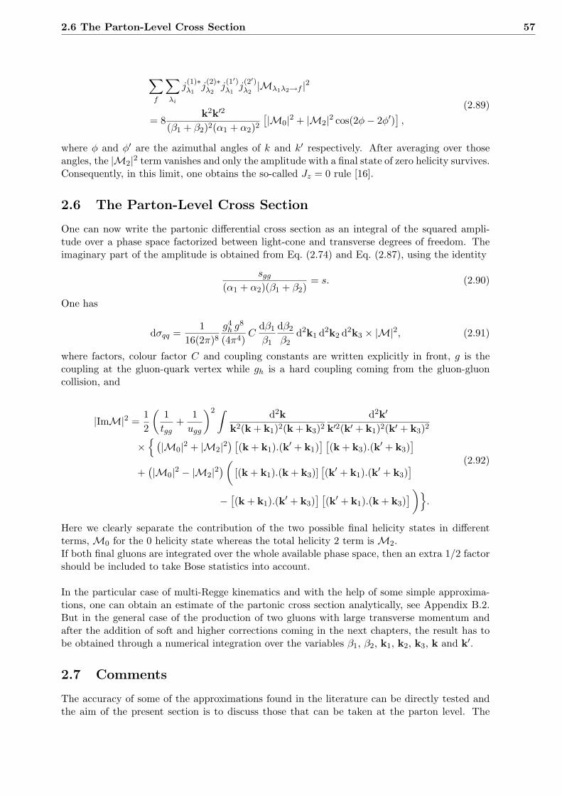
2.6 The Parton-Level Cross Section 57

∑f

∑λi

j(1)∗λ1

j(2)∗λ2

j(1′)λ1

j(2′)λ2|Mλ1λ2→f |2

= 8k2k′2

(β1 + β2)2(α1 + α2)2

[|M0|2 + |M2|2 cos(2φ− 2φ′)],

(2.89)

where φ and φ′ are the azimuthal angles of k and k′ respectively. After averaging over thoseangles, the |M2|2 term vanishes and only the amplitude with a final state of zero helicity survives.Consequently, in this limit, one obtains the so-called Jz = 0 rule [16].

2.6 The Parton-Level Cross Section

One can now write the partonic differential cross section as an integral of the squared ampli-tude over a phase space factorized between light-cone and transverse degrees of freedom. Theimaginary part of the amplitude is obtained from Eq. (2.74) and Eq. (2.87), using the identity

sgg(α1 + α2)(β1 + β2)

= s. (2.90)

One has

dσqq =1

16(2π)8

g4h g

8

(4π4)C

dβ1

β1

dβ2

β2d2k1 d2k2 d2k3 × |M|2, (2.91)

where factors, colour factor C and coupling constants are written explicitly in front, g is thecoupling at the gluon-quark vertex while gh is a hard coupling coming from the gluon-gluoncollision, and

|ImM|2 =12

(1tgg

+1ugg

)2 ∫ d2kk2(k + k1)2(k + k3)2

d2k′

k′2(k′ + k1)2(k′ + k3)2

×{(|M0|2 + |M2|2

) [(k + k1).(k′ + k1)

] [(k + k3).(k′ + k3)

]+(|M0|2 − |M2|2

)([(k + k1).(k + k3)]

[(k′ + k1).(k′ + k3)

]− [(k + k1).(k′ + k3)

] [(k′ + k1).(k + k3)

])}.

(2.92)

Here we clearly separate the contribution of the two possible final helicity states in differentterms, M0 for the 0 helicity state whereas the total helicity 2 term is M2.If both final gluons are integrated over the whole available phase space, then an extra 1/2 factorshould be included to take Bose statistics into account.

In the particular case of multi-Regge kinematics and with the help of some simple approxima-tions, one can obtain an estimate of the partonic cross section analytically, see Appendix B.2.But in the general case of the production of two gluons with large transverse momentum andafter the addition of soft and higher corrections coming in the next chapters, the result has tobe obtained through a numerical integration over the variables β1, β2, k1, k2, k3, k and k′.

2.7 Comments

The accuracy of some of the approximations found in the literature can be directly tested andthe aim of the present section is to discuss those that can be taken at the parton level. The


idea is to start with the reference curve of Fig. 1.12 and modify only the parton level part. Thefirst point is the claim that the calculation is perturbative and the second, the importance ofthe Jz = 0 rule as well as the contribution of the diagram where one of the final partons isemitted from the screening gluon.

One of the main assumptions [16] is the perturbative nature of the calculation. The argument isbased on the fact that the gluons involved in the loop have transverse momenta larger than 1 GeVbut this assumption can be checked. In the plot of Fig. 2.14, we show the distributions of dσ/d|k|

|k3||k1||k|

|ki| [GeV]

dσ

d|k

i|[n

b/G

eV]

54.543.532.521.510.50

1.6

1.4

1.2

1

0.8

0.6

0.4

0.2

0

Figure 2.14: Distribution of the transverse momentum |k|, |k1|, |k3| for the referencecurve at the TeVatron and Emin

T >10 GeV. Note that even if it is not aphysical observable it can be used to test properties of the theoreticalcalculation.

for the reference curve parametrisation at the TeVatron. One can directly see that the meanvalues are around 1 GeV. Although the distribution dσ/d|k| is not a physical observable, it isa useful quantity to test the assumptions used in the theoretical calculations. In addition, onecan also choose to define the perturbative quantity σpert as the value of the cross section inwhich gluon-transverse momenta squared k2, (k + k1)2, (k + k3)2 are larger than 1 GeV2 andcompute the ratio σpert/σ. This is done by cutting the momenta entering the gluon propagatorsand, for different jet transverse minimum energies, the result is given in Table 2.1. These small

Experiment EminT σpert/σ

CDF RunII 10 GeV 30%CDF RunII 35 GeV 20%

Table 2.1: Ratio σpert/σ where σpert is the value of the cross section if gluon-transversemomenta squared k2, (k + k1)2, (k + k3)2 are larger than 1 GeV. Differentexperiments and jet transverse minimum energies are presented but in allcases the parametrisation is the one of the reference curve.

numbers are due to the fact that transverse momenta k1 and k3 are comparable to k in ourmodel. Hence, they cannot be neglected and lead to three different cuts on the cross sectionthat reduce it substantially2.

2This conclusion changes slightly with the implementation of the Sudakov form factor as explained in Chap. 4but small momenta will keep contributing significantly to the cross section.

2.7 Comments 59

Note that as EminT increases the gluon loop gets softer. It can be explained by the fact that

at fixed proton energy, the production of high-ET jets requires larger longitudinal momentumtransfer. So, the effect of the non-perturbative region of QCD is not negligible and under thoseconditions, it should be interesting to consider modifications of the gluon propagators to takeinto account the non-perturbative aspect of the gluon loop. This was already done in differ-ent quasi-elastic models [12, 15], however, it remains unclear how to take these modificationsinto account in a consistent and gauge invariant way as changes to the propagators also implychanges to the vertices.

If the momentum in the loop k is small, one can ask if neglecting ki in front of k and k′ isaccurate. We show in Fig. 2.15.a the reference curve of Fig. 1.12 and the same curve if oneneglects ki. The approximation is very rough, leading to a factor 2 with respect to the referencecurve and to an overestimation of the cross section. Another current approximation is to keep

CDF data

Emin⊥ [GeV]

σ[n

b]

403530252015105

100

10

1

0.1

0.01

0.001

0.0001

(a)

Emin⊥ [GeV]

σ(J

z=

2)/σ

(Jz

=0)

[%]

403530252015105

4

3.5

3

2.5

2

1.5

1

0.5

0

(b)

Figure 2.15: (a) The effect of neglecting ki in front of k and k′. (b) Ratio be-tween σ(Jz = 2) and σ(Jz = 0) as a function of the jet transverseminimum energy. σ(Jz = 0) corresponds to the application of the Jz=0rule.

only the term that gives the helicity-0 contribution in Eq. (2.91), this is what is called the Jz = 0approximation. We confirm, as shown in Fig. 2.15.b, that the λ = 0 terms is dominant as noticedin [16], the λ = 2 term contributes only for 2-3% of the cross section. Nevertheless, we shallkeep it in the following studies in order to be as complete as possible.

Finally, there is the complicated question of the second diagram of Fig. 2.10. One knows thatits contribution to the amplitude should be small as it contains one more hard propagator.

2.7.1 The Second Diagram

The calculation of the amplitude of the second diagram where the two gluons are emitted fromdifferent t-channel legs cannot be made in the same way as one doesn’t have the gg → gg irre-ducible vertex. Nevertheless, it can be evaluated with the help of the Lipatov vertices [44, 79]in multi-Regge kinematics. We present here our result.

One has to start with the diagram of Fig. 2.16 and calculate


q − k1

k2 − k3

k1 − k2

q

p p + k3

k k + k1

k + k2 − k3

p + k

q − kk + k2

Figure 2.16: Kinematics of the diagram with final gluons emitted from different legsin the t-channel.

ImM2 = sg2h g

4

(2π)2

δc1c2

4N

∫d2k

k2(k + k1)2(k + k2)2(k + k2 − k3)2

× Cµ11 (k + k1, k + k2)Cµ2

2 (−k1,−k − k2 + k3) e∗µ1(λ3)e∗µ2

(λ4).(2.93)

The main part is the evaluation of contractions of Lipatov vertices [44, 79] with the polarisationvectors e∗µ1

(λ3)e∗µ2(λ4), e.g. for the first vertex, between

Cµ11 (k + k1, k + k2) = qµ

(β1 − 2

(k + k1)2

α1s

)−pµ

(α1 − 2

(k + k2)2

β1s

)−(2k+k1+k2)µ, (2.94)

following the kinematics of Fig. 2.17, and

e∗µ1(λ3) =

1√2

0

λ3 cos(θ)−i

−λ3 sin(θ)

, (2.95)

where λ3 is the helicity of the emitted gluon and θ its polar angle in the center-of-mass frameof the collision. Obviously, this calculation is interesting in itself and the method is detailed

k1 − k2

k + k1

k + k2

k2 − k3

k

k + k2 − k3

Figure 2.17: Kinematics of the Lipatov vertices.

in Appendix B.2.5, we directly present the results here. The first Lipatov vertex gives

Cµ11 e∗µ1

(λ3) =√

2|k + k1||k + k2||k1 − k2| λ3e

−iλ3φ12 , (2.96)

while the second gives

2.7 Comments 61

Cµ22 e∗µ2

(λ4) = −√

2|k||k + k2 − k3||k1 − k2| λ4e

−iλ4φ23 , (2.97)

where φij is the angle between the vectors. Using the above results, one can now compute thecross section by squaring the amplitude, so that

|M2|2 =∫

d2kk2(k + k1)2(k + k2)2(k + k2 − k3)2

d2k′

k′2(k′ + k1)2(k′ + k2)2(k′ + k2 − k3)2

× |k + k1||k + k2||k1 − k2|

|k + k2||k + k2 − k3||k1 − k2|

|k′ + k1||k′ + k2||k1 − k2|

|k′ + k2||k′ + k2 − k3||k1 − k2|

×∑λ3λ4

(−2λ3λ4)(−2λ′3λ′4)e−iλ3φ12−iλ4φ23eiλ

′3φ′12+iλ′4φ

′23 .

(2.98)

The main characteristics of the second diagram appears here, in the exponential factor. Since ifthe angles are identical then only the amplitudes with gluons of identical helicity λ3 = λ4 in thefinal state survive. Actually, in the limit of ki � k2, this condition is fulfilled and only processeswith helicity 2 contribute to the cross section. Assuming that it is the dominant part, one cansum over the possible helicity states in the same spirit as what was done in the first diagramand one obtains

|M2|2 =16

|k1 − k2|4∫

d2kk2(k + k1)2(k + k2)2(k + k2 − k3)2

d2k′

k′2(k′ + k1)2(k′ + k2)2(k′ + k2 − k3)2

× [fc(k)fc(k′) + fs(k,k′)] [

gc(k)gc(k′) + gh(k,k′)],

(2.99)

where the functions are defined by

fc(k) = (k + k1).(k + k2),gc(k) = k.(k + k2 − k3),

(2.100)

fs(k,k′) = (k + k1).(k′ + k1)(k + k2).(k′ + k2)− (k + k1).(k′ + k2)(k + k2).(k′ + k1),gh(k,k′) = k.k′(k + k2 − k3).(k′ + k2 − k3)− k.(k′ + k2 − k3)(k + k2 − k3).k′.

Finally, we gather all the coefficients in front and the differential cross section for the seconddiagram is

dσ =g4hg

8

4π4(2π)8

N2 − 12N

1|k1 − k2|4

dβ1

β1

dβ2

β2d2k1d2k3d2k2 × |M2|2. (2.101)

Note that one could have evaluated the first diagram in the same way, i.e. by successive con-tractions of the active gluon momenta with the corresponding Lipatov vertices, and recover thefinal expression of Eq. (2.91) for the first amplitude.

The contribution to the cross section can now be evaluated numerically after the introductionof an impact factor to regulate the IR divergence. Without any other higher-order correctionsthat should decrease its importance, the second diagram accounts for 15% of the first diagramcross section with all corrections included and Emin

T >10 GeV. In addition, the final dijet systemis of helicity 2 and can be differentiated from the dominant contribution of the first diagramthat has a total helicity 0. Consequently, the interference between the two diagrams is almostzero and will not be discussed here.


It is usually assumed that the extra gluon in the t-channel is needed only to screen the colourexchange and does not participate to the hard subprocess. Because of that, pomeron fusionis very similar to gluon fusion and the details of the final state of the hard interaction do notsubstantially change the calculation. In particular, one can change the hard subprocess withouttouching the rest of model. This also makes the calculation of the dijet quasi-elastic produc-tion similar to that of the Higgs boson quasi-elastic production and leads to the hope thatthe CDF data can be used to calibrate Higgs boson production.

This is where the lowest-order perturbative QCD calculation ends. The first correction thatcomes is the introduction of an impact factor that embeds the quarks into a proton to reproducea typical collision at a hadron collider.

Chapter 3

The Impact Factor

The previous description of the dijet cross section considers only the parton-level amplitudewhere the final system is produced after the interaction of two quarks. Besides, the expressionof Eq. (2.91) is singular when the exchanged gluons go on-shell, i.e. k2, (k + k1)2, (k + k3)2,k′2, (k′ + k1)2, (k′ + k3)2 → 0. The following chapter presents two ways of embedding theparton-level gluon production into a proton-proton collision and takes care of the singularity bythe introduction of an impact factor. The first section gives the general properties of this object.The second section develops a simple approach to the description of ultra-relativistic protonswhile Sec. 3.3 is devoted to the construction of an impact factor coming from unintegrated gluonsdensity (UgD). Actually, the results of Chap. 2 have shown that the parton-level calculation isdominated by the non-perturbative region, i.e. the active and screening gluons can be very soft.Consequently, one has to carefully treat the soft part and this is one of the advantage of thepresent parametrisation that allows to consider it separately. Finally, both impact factors werebuilt using parameters coming from data, a fit to the elastic cross section in the first case andto the gluons density in the second.

3.1 General Properties of Impact Factors

The hadron impact factor comes naturally from the fact that in a real process, the quarks be-tween which the pomeron is exchanged are embedded into a hadron1. The impact factor Φ isthe object that one should convolute with the parton level cross section to obtain the hadronicone and is pictured in Fig. 3.1. It is related to the partonic content of the proton and gives the

kk + k1

k + k3

Φ

Φ

Figure 3.1: Gluon dijet production now embedded in proton-proton scattering.

probability amplitude of interaction between its constituents and the exchanged particles in the

1We consider here the general case. In the following we shall focus on proton-proton collisions that are typicalof the LHC but it also applies for proton-antiproton collisions at the TeVatron.

64 The Impact Factor

t-channel. It also includes the expected energy behaviour of the cross section for this type ofscattering.

Hadrons are colourless objects, so that if the gluon exchanged is very soft, its correspondingwavelength is too large to resolve the initial particle that appears colourless, without colouredconstituent to couple with2. The argument can be expressed, according to [80, 81], as gluonswith wavelength λ average the colour of the hadron, and hence a suppression proportional to r/λmust always be present when coupling to a colour singlet of size r. In two-gluon exchange, thisproperty comes from the hadron impact factor Φ(ka,kb), which is such that

Φ(0,kb) = 0 = Φ(ka, 0), (3.1)

where ka and kb are the transverse momenta of the two t-channel gluons. Consequently, thedifferential cross section for gluon dijet production of the previous chapter, now embedded inproton-proton scattering, is

dσ = dσqq ⊗∏i=2±1

Φ (k,−(k + ki)) Φ(k′,−(k′ + ki)

). (3.2)

The impact factor has to be inside the loop integral over k and k′. This first correction to theparton-level calculation also removes all infra-red singularities due to the fact that the impactfactor goes to zero with the propagators. However, it has been argued that the divergence couldbe regularised via the Sudakov form factor [16], another correction discussed in Chap. 4. Veryroughly, the Sudakov factor comes from virtual vertex corrections and exponentially suppressesthe amplitude as the momentum in the loop becomes small. Thus it also makes the momen-tum integration infrared safe. One can see that it is not sufficient as the same diagram alsocontributes to the inclusive jet production which does not contain any Sudakov form factor butmust be finite nevertheless. The source of the cancellation should be elsewhere, in the protonimpact factor. It is why in the present work, the colour neutrality of the incoming hadrons isimplemented separately from the Sudakov correction. This is different from the Durham modelthat defines the impact factor via a unintegrated gluon density that includes the Sudakov factor.Here, the idea is a little different as we do not use directly the unintegrated gluon density butan impact factor build in such a way that soft and hard emissions from the proton are treatedin the same object. The impact factor is tuned to data to model the behavior of the proton andis supposed to include all corrections, and in this picture the Sudakov form factor is anotherpiece of the calculation.

We present here two different manners to implement the impact factor in the calculation. Thefirst one is a really simple impact factor that describes the proton in terms of the quark light-conewave function. The second is based on a differentiation of usual parton distribution functionand includes a dependence on the longitudinal momentum fraction lost by the proton.

3.2 Impact Factor from a Quark Model

An approach to the impact factor is to consider that an ultra-relativistic proton is made of3 quarks to which the exchanged gluons couple. According to references [80] and [82], one canderive an impact factor in terms of the quark light-cone wavefunction (LCWF).

The first assumption is that the proton is dominated by a 3-quark Fock state. In this case, itwas shown that the impact factor corresponding to two gluons of momenta ka and kb couplingto the proton is divided in the two diagrams of Fig. 3.2. The function E1 corresponds to the first

2This can be seen the other way around: a hadron cannot emit gluons with wavelength greater than its size.

3.2 Impact Factor from a Quark Model 65

ka kb ka kb

Figure 3.2: The two contributions to the LCWF impact factor.

one, where the two exchanged gluons are attached to the same quark and one can show that itis identical to the measured Dirac elastic form factor in γ∗p scattering

E1 (ka + kb) = F1(t) =3.53− 2.79t

(3.53− t)(1− t0.71)2

, (3.3)

with t = − (ka + kb)2. This fits the data [83] for |t| smaller than 9 GeV2. In order to build the

complete impact factor, one has to add the contribution of the coupling of gluons to differentquarks, E2 (ka,kb) which has the property

E2 (ka, 0) = F1(−k2a). (3.4)

Hence, one can use a simple parametrization which takes into account the above statement,

E1 (ka + kb) = F1

[−(ka + kb)2],

E2 (ka,kb) = F1

[−(k2a + k2

b + cka.kb)],

(3.5)

where c is a free parameter that is of the order one in the proton case. The impact factor nowreads

ΦLCWF(ka,kb) = 3[F1

(−(ka + kb)2)− F1

(−(k2a + k2

b + cka.kb))]. (3.6)

This makes the dijet cross section finite. The factor 3 in front approximately gives the quarkcounting rule that says that hadronic cross sections are proportional to the number of valencequarks in the colliding particles.

The LCWF impact factor of Eq. (3.6) has no energy dependence but it can be easily introducedgoing back to the phenomenological description of pomeron exchange in the S-matrix formalismof Sec. 1.3.1. One can include the s behaviour of the cross section via a Regge factor [84]

Ri =(s

si

)α(ti)

. (3.7)

The Regge trajectory of the pomeron is α(ti), s is the energy in the center-of-mass frame of thesystem and si, ti with i=2± 1 are the Mandelstam invariants of the upper and lower part of thediagram as shown in Fig. 3.3.


t1

t3

s1

s3

s

Figure 3.3: Decomposition of the main diagram in two parts according to [84]. Bothsubdiagrams have their own Mandelstam invariants si and ti for i=2±1.

One has for the upper proton of the process of Fig. 2.10

Φp1

LCWF(k,−(k+k1)) = 3(s

s1

)α(t1) [F1

(−k21

)− F1

(−(k2 + (k + k1)2 − c (k + k1).k))]. (3.8)

In the kinematics of Fig. 3.4, one can calculate s1 and t1 using the four-momentum of the

q − k1

k2 − k3

k1 − k2

q

p p + k3

k

k + k1

k + k3

k + k2

Figure 3.4: Kinematics of two-gluon production.

centrally produced system

kµX = (k1 − k2)µ + (k2 − k3)µ

= (α1 + α2)pµ + (β1 + β2)qµ + (k1 − k3)µ,(3.9)

that leads to

s1 = (q − k1 + kX)2

= (β1 + β2)s,

t1 = (q − q + k1)2

= −k21,

(3.10)

in the large s limit. One can directly note that s1 is proportional to the longitudinal momentumlost by the incoming hadrons and the same can be done for the bottom proton. Finally the

3.2 Impact Factor from a Quark Model 67

coefficients c and the normalisation of the cross section can be fixed using soft data as explainedin the next section.

3.2.1 Finding the Parameters of the Model

The previous model for the proton impact factor is also valid for other quasi-elastic or elasticprocesses. For instance, the elastic cross section calculation from the exchange of a pomeronmodeled by two gluons, can be performed and compared to the data in order to fix the param-eters.

The elastic cross section of Fig. 3.5, in the same framework and kinematics as the dijet produc-tion, is

k k + k1

Φ

Φ

Figure 3.5: High-energy elastic cross section. The pomeron exchange is modeled by atwo-gluon exchange in the same framework as the dijet production.

σel = g8 481π2

∫d2k1

∫d2k

k2(k + k1)2ΦLCWF (k,−(k + k1)) ΦLCWF (−k, (k + k1))∫

d2k′

k′2(k′ + k1)2ΦLCWF

(k′,−(k′ + k1)

)ΦLCWF

(−k′, (k′ + k1)),

(3.11)

This result can be compared with available data on total and elastic cross sections, assumingthat at high-energy those two are due to pomeron exchange only. Using the E710 result [85] leadsto the values of the coefficient c = 0.61 and the normalisation is obtained through the use of aneffective soft coupling g =

√4πα with α = 0.88. This value replaces g in Eq. (2.91). The authors

of [82] obtain a fit to less than 10% and their results have been checked here. It was also shownthat the curvature of the differential elastic cross section dσ/dt within this model is too large,and implies the importance of the non-perturbative regime of QCD in the region of small |t|.The use of perturbative exchange is thus tentative at best to estimate the value of the parame-ters3. Another inconvenient of the method is that one had to postulate that the soft amplitudeis dominated by the exchange of simple poles. Even if it is true at the TeVatron energy, onecan have non-negligible corrections going to LHC that cannot be taken into account at this level.

The LCWF model is simple and possesses all needed ingredients, i.e. a dependence on thetransverse momenta and on the energy in the center-of-mass frame. The problem of the curvaturecan be solved by introducing by hand a t-dependence, as it is done in the Durham model.However, it relies on non-perturbative cross sections to fix its input. It may be better to use analternative model fitted to deep inelastic scattering (DIS) and photoproduction data, this is theidea behind unintegrated gluons density discussed in the next section.

3Note that the authors of [82] demonstrate that the introduction of non-perturbative effects through a modi-fication of the gluons propagator as described in Sec. 1.3.3 improves the t-slope.


3.3 The Unintegrated Gluon Density

From the study of deep inelastic scattering at HERA, one can extract information about theparton content of the proton. In the standard approach, the gluon distribution depends onlyon longitudinal momentum fraction but we are looking for the emission of gluons with non-negligible transverse momenta. Moreover, in our case, the exchanged gluons can be very soft sothat one could be interested to extend the description of the impact factor to the region wherethe DGLAP evolution breaks down. In the present section, we shall use the parametrisation ofthe impact factor described in [86] that solves these two issues and we present an impact factorthat depends both on the longitudinal momentum lost by the proton and on the transversemomenta of the t-channel gluons.

The distribution of gluons inside an ultra-relativistic proton can be modeled for diagonal pro-cesses, i.e no momentum transfer, by replacing the Born-level impact factor of the quark modelwith an impact factor ΦUgD based on the unintegrated gluon density F(x,k2) made of two parts.One drives the hard emission of gluons FHard and the second the soft emisions FSoft, in additionwith a smooth interpolation between them. We start with the perturbative exchange, i.e. theemission of large transverse-momentum gluons. In this case, the gluon content of the protonis described by the usual gluon distribution and as we are looking for the dependence in thetransverse momentum, the hard part of the impact factor comes from a direct differentiation ofthe gluon distribution [44, 45, 87]

FH1 =∂ xg(x,k2)∂ log(k2)

. (3.12)

6The gluon distribution function g(x,k2) is extracted from fits to DIS data. This work has beendone by the collaborations GRV [88], MRS [89] and CTEQ [90] and the fits are based on theDGLAP equation. The domain of validity of FHard is for k2 ≥ k2

c with k2c ' 0.9 or 1.4 GeV2

depending on the fit (see below). At small to moderate transverse momenta, one has to providea model for the unintegrated gluon density (UgD). An educated guess, based on colour-dipolephenomenology of hard processes at small-x [91–93], suggests that the interaction of perturbativegluons is similar to the Yukawa screened flux of photon in a quark dipole, up to a colour factorand a coupling constant, so that

FH2 =N2c − 12

αs(k2)π

(k2

k2 + µ2h

)2

F1(k2), (3.13)

where Nc is the number of colours. The scale µh is related to the propagation length of gluonsby µh = 1/Rh. Because of confinement, perturbative gluons do not propagate at large distancesand one can take Rh ' 0.27 fm according to lattice studies [94]. In this case, F1(k2) is theconventional quark dipole form factor

F1(k2) =1(

1 + k2

Λ2

)2 , (3.14)

where Λ is a free parameter set to 1 GeV and the strong coupling constant is frozen at αs=0.82in the infra red [95, 96]. One can now define the hard part of the impact factor by matching theDGLAP fits with the above dipole picture at kc and

FHard = FH2(k2) FH1

(x,k2

c

)FH2 (k2

c)θ(k2c − k2

)+ FH1

(x,k2

)θ(k2 − k2

c

). (3.15)

In the moderate transverse-momentum region, the hard impact factor shows consequently thesame x-dependence as the DGLAP fit at k2

c together with the k2-dependence of the dipole pic-

3.3 The Unintegrated Gluon Density 69

ture. The large-x behaviour is introduced via a purely phenomenological factor (1− x)5.

In the soft region, i.e. at small k, one has to deal with non-perturbative gluons interacting withlarge dipoles. The phenomenology of this soft exchange can be modeled in the spirit of thedipole picture of Eq. (3.13) at the tree-level

FSoft = asoftN2c − 12

αs(k2)π

(k2

k2 + µ2s

)2

F1(k2), (3.16)

where asoft is an adjustable parameter. The scale µ2s is, as previously, related to the propagation

length of gluons, but this time this is the propagation of non-perturbative gluons, so that µ2s �

µ2h because R2

s � R2h. Finally, the unintegrated gluon density can be written

F(x,k2) = FSoft ν2s

k2 + ν2s

+ FHard k2

k2 + ν2h

, (3.17)

with νs ' µh that insures that the soft component decreases fast in the hard region k2 > µ2h but

dominates in the soft one.

The above description of the unintegrated gluon density is a summary of reference [86] andwe want to underline that this density was build in a phenomenological way, and hence is notunique. It depends on several assumptions and choices. Some of the parameters, R2

h, kc andthe freezing of the strong coupling, are borrowed from the literature, but the others, asoft, µ2

s

and νh, were adjusted on available data from ZEUS [97–100], H1 [101–103], E665 [104] andNMC [105] in the ranges 0 ≤ |k2| ≤ 35 GeV2 and x ≤ 10−2. Actually, one has four differentfits which give similar chi-square when fitting to the data and, in particular, the details of thenon-perturbative region are different. All hard inputs are taken from LO GRV98 parton distri-butions apart for Fit-3 that comes from a functional form of FH1 . The main difference betweenthe fits is in the parametrisation of the soft region for which the parameters were adjusted ondata using different fitting techniques. As an example, we show in Fig. 3.6 the hard and soft

HardSoft

Total

x=10−2

k2 [GeV2]

F(x,k

2)

[Fit

-1]

10310210110010−110−2

101

100

10−1

10−2

(a)

HardSoft

Totalx=10−4

k2 [GeV2]

F(x,k

2)

[Fit

-1]

10310210110010−110−2

102

101

100

10−1

10−2

(b)

Figure 3.6: Fit-1 parametrisation of the unintegrated gluon distribution as a functionof k2 at fixed x. (a) x=10−2 and (b) x=10−4. The plots present thedifferent contributions FHard, FSoft and their sum.

parts of the Fit-1 unintegrated distribution as a function of k2 and for two values of x. One candirectly note that both plots show a dip at the interface between the hard and soft component.


This comes from the fact that the components are clearly separated but with a small extrapo-lation of the soft part into the hard part as well as of the hard into the soft. After integrationover k2 one finds the correct description of F2p in agreement with data.

The other fits have a similar behaviour despite the differences in the parametrisation of the softregion and are shown in Fig. 3.7, Fig. 3.8 and Fig. 3.9. The main remark is that the importanceof the non-perturbative contribution in Fit-4 is extended to larger k2 in this case even if bothparametrisations exhibit the same behavior at small and large k2.

HardSoft

Total

x=10−2

k2 [GeV2]

F(x,k

2)

[Fit

-2]

10310210110010−110−2

101

100

10−1

10−2

(a)

HardSoft

Total

x=10−4

k2 [GeV2]

F(x,k

2)

[Fit

-2]

10310210110010−110−2

102

101

100

10−1

10−2

(b)

Figure 3.7: Fit-2 parametrisation of the unintegrated gluon distribution as a functionof k2 at fixed x: (a) x=10−2 and (b) x=10−4. The plots present thedifferent contributions FHard, FSoft and their sum.

HardSoft

Total

x=10−2

k2 [GeV2]

F(x,k

2)

[Fit

-3]

10310210110010−110−2

101

100

10−1

10−2

(a)

HardSoft

Total

x=10−4

k2 [GeV2]

F(x,k

2)

[Fit

-3]

10310210110010−110−2

102

101

100

10−1

10−2

(b)


3.3 The Unintegrated Gluon Density 71

HardSoft

Total

x=10−2

k2 [GeV2]

F(x,k

2)

[Fit

-4]

10310210110010−110−2

101

100

10−1

10−2

(a)

HardSoft

Total

x=10−4

k2 [GeV2]

F(x,k

2)

[Fit

-4]

10310210110010−110−2

102

101

100

10−1

10−2

(b)


3.3.1 Impact Factor from the Unintegrated Gluon Density

The above fits to the data allow to model the impact factor at non-zero momentum transfer andfor different longitudinal momentum fractions. The kinematics used in the present description isshown in Fig. 3.10. In the studied case of quasi-elastic production, the two gluons have different

(xa,ka)

Φ

(xb,kb)

Figure 3.10: General picture of the kinematics used in the present description of theimpact factor.

longitudinal momentum fractions, the screening gluon can be very soft and one has xa � xb asshown by the conditions (2.55) and (2.64).

According to [106, 107] the skewed distribution can be related to the forward distribution by

Fskewed

(xa � xb, xb,k2

)= Rg F

(xb,k2

), (3.18)

The skewness factor Rg can be effectively taken into account by rescalling the x at which the UgDis calculated. Assuming that F(xb,k2) ∝ x−λ with λ the effective intercept, one has

Rg

(1x

)λ=(

1c(λ)x

)λ. (3.19)

It appears that the factor c(λ) has little dependance on the intercept and consequently one canchoose to fix it at the mean value < c(λ) >= 0.41, so that

Fskewed

(xa � xb, xb,k2

)= F (0.41xb,k2

). (3.20)


The second problem is the non-zero transverse momentum transfer. This is introduced via auniversal exponential factor constructed in such a way that it respects condition (3.1), includesthe shrinkage and the t-dependence of the impact factor. The first condition is realised withthe help of a prefactor f(ka,kb) that goes to zero with one of its arguments and is equal to 1 ifka = kb. It can be choosen as

f(ka,kb) =2k2

ak2b

k4a + k4

b

, (3.21)

in addition with the prescription

φ (xa � xb, xb,ka,kb) =4π2

g2

N2c − 12Nc

F(

0.41xb,(

ka + kb2

)2)f(ka,kb), (3.22)

that models the distribution of gluons inside an ultra-relativistic proton and in this prescriptionthe soft coupling g is absorbed into the definition of F .The t-dependence is usually taken into account by an exponential. According to studies ofdiffractive vector meson production [86], one can take

Φ = φ× e− 12B(x)|t|,

B = B0 + 2α′ lnx0

x.

(3.23)

Here, B0 = 4 GeV−2, α′ = 0.25 GeV−2 and x0 = 3.4 10−4 are chosen to reproduce the correct |t|-slope of the cross section. The energy dependence is inspired by the Regge phenomenology ofpomeron exchange of Sec. 1.3.1 and was tested on diffractive vector-meson production [108].Using these values of the diffractive parameters, the logarithmic t-slope of the distribution isapproximately equal to B ' 4 GeV−2. This is significantly smaller than the slope in elasticproton-proton collision at the TeVatron energy, that is

dσelasticpp

d|t| ∝ e−2Bel|t|, (3.24)

where Belastic ' 8.5 GeV−2. The present choice of B is more natural than B ' Bel since elasticscattering at the TeVatron probes the gluon distribution at very small x, of the order x ∼ 10−7,while in our process the energetic gluons carry only ' 10−2 of the proton momentum. Thischoice is model-dependent and introduces an extra uncertainty into theoretical calculations ofthe quasi-elastic cross sections.

The complete UgD-based impact factor incorporates now all the ingredients requested and yields

ΦUgD (xa � xb, xb,ka,kb) =4π2

g2

N2c − 12Nc

F(

0.41xb,(

ka + kb2

)2)× 2k2

ak2b

k4a + k4

b

e− 1

2(B0+2α′ ln

x0xb

)|t|.

(3.25)This function replaces ΦLCWF, as shown in Appendix A. After the considerations of Chap. 2 thathave shown that an important part of the exchanged gluons are soft and that the calculation issensitive to the details of the non-perturbative regime of QCD, one must note that the presentimpact factor is somewhat uncertain. One of its advantages is that it treats separately the softand hard regimes and the parametrisation is just an attempt to describe phenomenologically theimpact factor. Here, we want to underline that a good agrement of the fit to small, moderate andlarge transverse momentum is not trivial, and that below x = 10−2 the accuracy is comparableto the one of the standard leading-order GRV fits.

3.4 Results and Conclusion 73

3.4 Results and Conclusion

We have presented two possible parametrisations of the impact factor, based on a simple light-cone wave function or on the unintegrated gluon density. Both of them depend on the transversemomentum of the exchanged gluons and on the longitudinal fraction lost by the proton. We shallnow define the variables in the particular kinematics of quasi-elastic production and show whatare the effects of the choice of different parametrisations on the dijet quasi-elastic production.

The parton-level cross section calculation, embedded into proton-proton exchange is givenby Eq. (3.2) and if one want to use ΦUgD, the longitudinal fraction lost by the upper proton isthe longitudinal fraction of k1, given by

kµ1 =−k2

1

(1− β1)spµ +

(k3

(1− α2)s+ β1 + β2

)qµ + kµ1 , (3.26)

hence xb = β1 + β2 in the kinematics of Sec. 2.4 and neglecting all terms of order O(1/s). Itcan also be taken directly from the four-momentum of the final system X of Eq. (3.9) since thetransferred momentum |t| is equal to |t1| as in Eq. (3.10). Consequently, the impact factor basedon UgD of the upper proton is

Φp1

UgD (z, (β1 + β2),k, (k + k1)) =4π2

g2

N2c − 12Nc

F(

0.41(β1 + β2),(

k + (k + k1)2

)2)

× 2k2(k + k1)2

k4 + (k + k1)4e− 1

2(B0+2α′ ln

x0β1+β2

)|k21|.

(3.27)

In the case of the lower proton, one finds

xb = α1 + α2,

t3 = −k23.

(3.28)

Fig. 3.11.a presents the reference curve for the two choices of impact factor.

403530252015105

100

10

1

0.1

0.01

0.001

0.0001

CDF dataLCWF

UgD

Emin⊥ [GeV]

σ[n

b]

(a)

Fit-4Fit-3Fit-2Fit-1

CDF data

Emin⊥ [GeV]

σ[n

b]

403530252015105

100

10

1

0.1

0.01

0.001

0.0001

(b)

Figure 3.11: Comparison of the impact factor. (a) LCWF stands for the light-cone-wave function impact factor and the band corresponds to the parametri-sations of the unintegrated gluon density. (b) The four different fitsof ΦUgD.


Although both lead to an acceptable fit to the data, the curvature of ΦUgD seems to be better.The band represents the four parametrisations of impact factor based on unintegrated gluon den-sity that only differ by the description of the soft coulour-singlet exchange. A look at Fig. 3.11.b,that gives the results for the four different types of parametrisations, shows that the Fit-4 withthe extended soft region gives the highest prediction.

The fact that one cannot fix the correct parametrisation of the impact factor using theoreticalarguments introduces an uncertainty on the results. By comparing the different prescriptions,the present study shows that the choice of the impact factor amounts to an uncertainty of atleast a factor 3 between the lowest and the highest curves.

Chapter 4

The Sudakov Form Factor

The central system produced in quasi-elastic processes comes from the scattering of two near-shell gluons and it is known that this kind of process has large logarithmic vertex corrections,which may be resummed to form the Sudakov form factor. One expects these corrections tolead to a substantial suppression of the cross section. This chapter describes different aspectsof the Sudakov form factor and several comments are in order.After the general definition, we shall discuss different open questions concerning the details ofthe Sudakov form factor as, in the dijet case, there exists no complete calculation to fix preciselythe scales. Hence it brings large uncertainties on the final cross section. We shall start with thescales, then discuss the importance of the subleading logs and of the constant terms structure.We also explain how it is possible to evaluate the mean value of the loop momentum using thesaddle point approximation and we shall confirm that the calculation is dominated by the non-perturbative region. We also briefly discuss the idea that non-standard diagrams may modifythe final result for the quasi-elastic dijet cross section. All these pieces will be brought togetherin the last section that summarises the uncertainties and demonstrates that the Sudakov formfactor is far from being under theoretical control.

4.1 General Definition of the Resummation

The present process is a typical case of the propagation of a gauge field from a long-distance con-figuration to a short-distance one, i.e. a soft scale to a hard scale. It was shown in [109, 110] thatone expects large doubly logarithmic corrections from virtual diagrams such as those of Fig. 4.1.The Sudakov corrections have been evaluated in QCD [111] and for on-shell initial gluons, theydiverge. However, in quasi-elastic processes, the initial gluons are slightly off-shell so that theirvirtualities provide a natural IR cut-off and the logarithms are large but finite. The presentsection gives the general properties of the Sudakov form factor and we shall try to explain howit can be calculated in QCD, the complete calculation is far beyond the scope of the thesis andhence, we just present the main lines1.

One can consider the one-loop correction to the vertex shown in Fig. 4.1.b. This diagramincludes an integral over the momentum in the loop, q, and in particular over both the frac-tion of light-cone momentum z and the transverse momentum q2. The integration builds updouble logarithms in the kinematical region where the virtual emission is soft and sandwichedbetween a soft and a hard scale, respectively `2 and µ2. As shown by Dokshitzer, Dyakonov and

1Sometimes, the Sudakov form factor is reworded using a Monte-Carlo language as the probability that thegluons in the t-channel do not emit extra partons. In this way, one has to subtract from unity the probabilitythat the hard subprocess is accompanied by a certain number of secondary partons. However, we prefer to keepthe original definition of the Sudakov form factor as a vertex correction.

76 The Sudakov Form Factor

(a)

q

(b)

Figure 4.1: (a) A higher-order diagram for quasi-elastic production that leads to largedoubly logarithmic corrections in the Feynman gauge. (b) The Sudakovform factor viewed as virtual vertex corrections.

Troyan (DDT) [111], at higher order, the leading double logarithms exponentiate. The expo-nentiation is the QCD analog of the form factor discovered by Sudakov in QED. The main issueis that one is dealing here with loop momenta that lie in the non-perturbative region and it isthen difficult to go beyond the leading-log approximation. However, DDT interestingly noticedthat the log structure appears from equations that look like bremsshtrahlung emission with thesame splitting function as those used in the DGLAP equation. Actually, if one looks at the crosssection level, the logarithmic IR divergences of bremsshtrahlung diagrams are canceled by thedivergences of virtual corrections, making the inclusive cross section finite, this is pictured inFig. 4.2. Hence, the inclusive cancellation of the IR divergences leads to the conclusion that the

+ = Finite

Figure 4.2: The logarithmic IR divergence of bremsshtrahlung diagrams is canceledby the divergence of virtual corrections, making the inclusive cross sectionfinite. This suggests that the log structure of virtual corrections is identicalto that of real emissions.

log structure of virtual corrections is identical to that of real emissions, that can be calculatedperturbatively in the DGLAP formalism. One can then write for the Sudakov form factor T thefollowing expression [16, 17]

T (µ2, `2) = e−S(µ2,`2),

S(µ2, `2) =∫ µ2

`2

dq2

2παs(q2)

q2

∫ 1−∆

0dz [zPgg +NfPqg] ,

(4.1)

that should be convoluted with the cross section of Eq. (3.2):

M(p1p2 → p∗1 + gg + p∗2) =Mqq ⊗ Φ(p1)√T (µ2, `21) Φ(p2)

√T (µ2, `22). (4.2)

Once again, we insist on the fact that the Sudakov form factor is a correction independent of theimpact factor and is hence not introduced in a derivative as in models that uses simple parton

4.1 General Definition of the Resummation 77

distribution function for the proton. The first integral of Eq. (4.1) refers to the transversemomentum of the particle in the loop q2 and αs(q2) is the strong coupling constant. Theintegration variable runs between `2i and µ2, naturally related respectively to the soft and hardscales between which the colour gauge field is developed. So, `i is linked to the virtuality of theinitial gluons (k + ki)2, depending on whether one deals with the upper or the lower part ofthe production diagram, that sets the scale from which an extra parton can be emitted, while µis related to the hard transverse scale k2 of the hard subprocess. The problems attached tothe definition of the scales is addressed in Sec. 4.2.1. The second integral is over the light-conemomentum z, ∆ is a cut-off discussed below, Nf is the number of flavours and Pgg, Pqg are theunregularised splitting functions2. One has

Pgg = 2Nc

[z

1− z +1− zz

+ z(1− z)],

Pqg =12[z2 + (1− z)2

],

(4.3)

where Nc is the number of colours. Note that the original prescription of DDT gives a slightlydifferent result as discussed in Appendix B.3. The origin of the double-log is in the first termof Pgg since the other terms will only give simple logs and constant terms. Here, a secondproblem appears as the argument is that virtual logarithmic divergences of bremsshtrahlungdiagrams are identical to the logarithmic divergences of the virtual diagram and it is knownthat those logs exponentiate, but the constant terms are not the same and nothing proves thatthey exponentiate. We leave this topic for Sec. 4.2.2 as the Sudakov correction is well definedin the regime where the logs are large and in particular when the double-log contribution isdominant. In order to obtain a quantitative idea of this factor one can work in the double log-approximation (DLA) of S(µ2, `2) that is computed by keeping only the term of interest afterthe integration over z,

SDLA(µ2, `2) =3π

∫ µ2

`2d2q

αs(q2)q2

log(

1|∆|). (4.4)

All details of the integration over z can be found in Appendix B.3. For the purpose of thedemonstration, one can fix the coupling constant to αs(µ2) in Eq. (4.4) and evaluate the secondintegral that depends on the choice of ∆. First, pure DGLAP kinematics [111] leads to thecut-off ∆ = q2/µ2 and one obtains

SDLA(µ2, `2) =3αs(µ2)

2πlog2

(µ2

`2

). (4.5)

However, it can be argued that the coherent effects lead to angular ordering in the successivesplitting of the secondary partons [112–114]. This ordering introduces a more restrictive limiton the z integral, which becomes linear in |q| leading to ∆ = |q|/µ. This result is also obtainedby the authors of [20, 112] who compute explicitly the next-to-leading-order (NLO) calculationof the relevant virtual corrections3. With this definition of the cut-off, one obtains a double-logresult which is a factor of two smaller than Eq. (4.5)

SDLA(µ2, `2) =3αs(µ2)

4πlog2

(µ2

`2

). (4.6)

2Note that the splitting function Pgq is not present as one deals only with gluons in the initial state.3We don’t want to enter into the details here, but one can note that, together with Eq. (4.1), it can also be

derived from the CCFM equation [115, 116].


Numerically this change is very substantial as it can lead to a factor O(10) in the cross section.In the following, all results are produced with the latter definition of ∆.

All choices, scales, cut-off and approximations will be studied and their effects on the value ofthe quasi-elastic dijet cross section tested in the final section where we show how sensitive theSudakov form factor is to those parameters.

4.2 Arbitrariness of the Sudakov Form Factor

From the point of view of the previous section, the Sudakov form factor seems to be undertheoretical control. However, as it suppresses the cross section by a factor of the order of 100to 1000, one can guess that we need to be very careful about its details. We would like todevelop four topics, i.e. the choice of scales µ2 and `2, the possibility to introduce a differentupper scale in the transverse and longitudinal integrals, the importance of the log contributionsversus the constant terms and the Sudakov form factor of non-standard diagrams.

4.2.1 Scales

At first sight, the Sudakov form factor depends on two scales that are the limits of the integralof Eq. (4.1). They are related to the soft and the hard scales of the process and we shall seethat the suppression factor is very sensitive to a change in their values. The order of magnitudeof both scales can be fixed from the kinematics but the theory doesn’t provide the coefficient inthe particular case of the two-gluon production.

As already mentioned, the lower limit `2 of the integral on transverse momentum must be ofthe order of the transverse momentum of the gluon that initiates the emission. In the presentpicture of the Sudakov form factor corresponding to virtual corrections at the vertex, this scaleis obviously of the order of (k + ki)2 with i = 2± 1. The status of the upper scale is a little bitmore complicated due to the fact that in the standard discussion of the Sudakov form factorsthe hard point-like vertex is characterized by only one scale, that is the mass of the producedsystem mX . In Monte Carlo language, this mass defines the phase space available for thesecondary parton emission which needs to be suppressed. Consequently, the upper scale shouldbe taken as µ = cmX with c a constant of order 1 and this is true for a point-like vertex.Nevertheless, in the dijet case, we enter a new kinematical regime as the two gluons can havelarge invariant mass

m2gg = sgg =

(β2k1 + β1k3 − (β1 + β2)k2)2

β1β2, (4.7)

both via large transverse momenta for which sgg ' k22 or via strong longitudinal ordering sgg �

k22. In Sec. 4.1, we have seen that a typical double-log-enhanced correction gets sizable logs

only if there is a large transverse momentum or large virtuality k22 inside the effective vertex,

or in other words, only if the effective vertex can be considered point-like. In this case, the flowof the transverse momentum q in the loop does not change the amplitude. On the contrary, ifthe vertex does not involve a sufficiently large scale, the momentum in the loop is enough toresolve the vertex and the transverse logarithm does not build up, leading to a complete changeof the log structure of the amplitude. The two situations are pictured in Fig. 4.3, and one canreasonably guess that the upper scale of the transverse integral is somewhat uncertain, but mustbe of the order of k2

2 as it marks the limit beyond which the double-logs do not build up. Withthis discussion in mind, we anticipate a little on the second part of the thesis, devoted to Higgsboson quasi-elastic production.According to [16, 17], one should have taken µ2 related to the quantity sgg. Actually, this is true

4.2 Arbitrariness of the Sudakov Form Factor 79

q2 ≪ k22

q2 ≃ k22

k22

Figure 4.3: The two different kinematical regime for dijet production. Left: Theeffective point-like vertex q2 � k2

2. Right: The resolved vertex q2 ' k22.

in the case of Higgs boson quasi-elastic cross section as the hard vertex is effectively point-like.The transverse momenta and virtualities of the top quarks inside the loop are larger or similarto the Higgs boson mass, so that the only available hard scale is indeed this mass squared. Inthe dijet case, one cannot neglect the new kinematical regime sgg � k2

2 and, in particular atTeVatron energy where k2

2 is of the order of the minimum transverse energy of the jet whichcan be as low as 10 GeV. Hence. according to the above discussion, we choose to fix the upperscale of the Sudakov form factor to

µ2 = k22/x, (4.8)

where x is an integer used to study the variation of the cross section with the details of theSudakov correction and thus the theoretical uncertainty on the numerical result.

The scale µ appears two times in Eq. 4.1, first as the upper limit of the transverse integralover q and second through the definition of ∆ in the upper limit of the longitudinal integralover z. One can then suggest to introduce different upper limits dealing with the longitudinaland the transverse pieces. The latter should be naturally related to the previous definition of µwhereas the former, denoted ν, should be linked to √sgg. For simplicity one can choose differenttransverse and longitudinal limits which become of the same order for purely transverse jets:

µ2 =k2

2

x, ν2 =

sgg4x. (4.9)

The effect of the additional scale on the dijet cross section is shown in Fig. 4.4,

Additional ScaleCDF data

Emin⊥ [GeV]

σ[n

b]

403530252015105

100

10

1

0.1

0.01

0.001

0.0001

Figure 4.4: Effect of the additional scale on the dijet cross section. The central plainline is the reference curve of Fig. 1.12.


that presents on the same plot the two cases, the addition of the second scale changes thecurvature in the high-mass region. Nevertheless, this change is small compared to the othersources of uncertainties and the error bars. The effect of the addition of a scale is not obviousbut it can be seen from the DLA form of the Sudakov form factor. One can compute thefunction SDLA of Eq. (4.4) but for ∆ = |q|/ν. It gives

S2scalesDLA ∝

∫ µ2

`2

dq2

q2log

ν

|q|= log

(`

µ

)log(`µ

ν2

),

(4.10)

after the calculation detailed in Appendix B.3.3. This expression has to be compared with theresult of Eq. (4.6)

SDLA(µ2, `2) ∝ log2

(µ2

`2

), (4.11)

and one can directly note that the dependence of S(µ2, `2) on the upper scale is strongly modified.Indeed, if µ starts increasing then one has now two opposite effects as log `µ

ν2 increases while log `µ

decreases. As shown in Fig. 4.5.a and 4.5.b, the dependence in the 2-scale case is rather different

Two scalesOne scale

µ [GeV]

S( ν

2=

102

GeV

2,ℓ

2=

1G

eV2)

10987654321

3.5

3

2.5

2

1.5

1

0.5

0

(a)

µ2 = k22

µ2 = 2k22

µ2 = 4k22

CDF data

Emin⊥ [GeV]

σ[n

b]

403530252015105

100

10

1

0.1

0.01

0.001

0.0001

1e-05

(b)

Figure 4.5: (a) Comparison of the dependence of the argument of the Sudakovform factor on the upper scale µ in the one-scale and two-scalescases. ν2=100 GeV2 and `2=1 GeV2, i.e. typical values of the quasi-elasticproduction are fixed. (b) Effects of a change in the upper limit µ on thecross section in the 2-scale case.

and a change in µ has then a less dramatic effect on the final result and on the uncertainty thataffects the calculation.

4.2.2 The Logarithmic Contribution and the Constant Terms

The validity of the formulae used here is based on the assumption that the log contributionsare dominant. However, the exact log contributions in the dijet case is not trivial and have notbeen fully calculated due to the additional difficulty described in the previous section. If theconstant term contribution is small, one can trust the exponentiation but we shall show that itis not the case in the energy domain considered. Furthermore, we have assumed that the impact


factor was similar to an integrated gluon density. In principle, the latter contains a Sudakovform factor inside the derivative of the gluon density. The derivation is performed in DIS butthe regime considered here, with a spectator gluon, is quite different and we believe we shouldinclude it outside the impact factor.

One can choose to keep the Sudakov form factor of Eq. (4.1) and to test the dominance ofthe logs. The sign and hierarchy of the different contributions can be obtained by an analyticcalculation in the approximation of fixed αs. According to Appendix B.3, one has

S(µ2, `2) ' αs2π

[6 log2 1

δ+ (−11 +

23Nf ) log

1δ

+ C

], (4.12)

where the term proportional to Nf is from Pqg and C gathers the non-leading log terms. Thisdecomposes the argument of the Sudakov form factor in three terms

S(µ2, `2) = αs

[a log2

(µ2

`2

)+ b log

(µ2

`2

)+ C

], (4.13)

namely, the double-log contribution, the single-log contribution and the constant term with a,b and C constant. In this approximation, the relative magnitude between the different terms isshown in Fig. 4.6 using ∆ = |q|/µ and for typical scales relevant for the CDF measurements.

Constant termslog2+log terms

log2 terms

ℓ [GeV]

S( µ

2=

102

GeV

2,ℓ

2)

43.532.521.510.50

12

10

8

6

4

2

0

Figure 4.6: Contribution of the various terms entering the argument of the Sudakovform factor in the approximation of fixed strong coupling and for µ2 =102 GeV2.

We remind the reader that µ is related to the mass of the dijet system and that `, the virtualityof the colliding gluons, is small.In the case of a running coupling, one has to perform a numerical calculation and the con-tributions are shown in Fig. 4.7 where we label the terms as in the fixed coupling case. Thefirst remark is that the picture is really different from what one expects, i.e. large double logcontributions and small constant terms. The single-log contribution is negative and eventuallyleads to a change of sign of the argument S(µ2, `2) if one neglects the constant term4. As weexplained in Sec. 4.1, the single-log contribution is not fully calculated in the dijet case and thefact that it is actually large makes the theoretical prediction particularly unstable. On top ofthis, one can also notice from Fig. 4.7 that the constant terms are numerically important, in

4Moreover, the negative contribution comes from Pgg and the positive one from Pqg.



log2 terms

ℓ [GeV]

S( µ

2=

102

GeV

2,ℓ

2)

43.532.521.510.50

12

10

8

6

4

2

0

-2

(a)


log2 terms

ℓ [GeV]

S( µ

2=

402

GeV

2,ℓ

2)

43.532.521.510.50

12

10

8

6

4

2

0

-2

(b)

Figure 4.7: Contribution of the various terms entering the argument of the Sudakovform factor. (a) µ2 = 102 GeV2 and (b) µ2 = 402 GeV2.

particular the logarithms are dominant only in the region ` � 0.5 GeV for µ = 10 GeV witha slight improvement if one takes µ = 40 GeV. With a running coupling, the log terms aredominated by the constant contribution with the consequence that one can trust the perturba-tive formula of Eq. (4.1) only in the non-perturbative region. Taking into account that, in thedijet quasi-elastic production processes, the mean value of ` is around 1 GeV, one might haveserious doubts about the validity of the Sudakov form factor in that context. In particular inthe fixed running coupling approximation for which the suppression factor is underestimated inthe small-` region leading to important consequences on the final cross section.We stress however that this result is model-dependent and as an example, we show in Fig. 4.8 the


log2 terms

ℓ [GeV]

S( µ

2=

102

GeV

2,ℓ

2)

43.532.521.510.50

12

10

8

6

4

2

0

Figure 4.8: Contribution of the various term entering the argument of the Sudakovform factor using the prescription for the cut-off, ∆ = |q|

|q|+µ .

same plot as the one of Fig. 4.7.a using this time the Durham prescription for the cut-off ∆ [117]

∆ =|q||q|+ µ

, (4.14)


that prevents the log contribution to go far below zero. One can also show that if we multiplythe upper scale by two, an assumption that is theoretically reasonable, the double log + singlelog contribution becomes always positive.

We now address the question of the constant terms. The exponential form of the Sudakov formfactor comes from the similarity of the log terms in the virtual and bremsshtrahlung diagrams,and it is known that the constant terms do not exponentiate. It is however assumed in most ofthe models that they are small. Consequently this introduces an additional uncertainty on thefinal result as the constant terms are not fixed by the theory and can vary. The effects of a simplechange are shown in Fig. 4.9. It corresponds to the multiplication by a factor 2 or 1/2 of all terms

0.5C2C

C=0CDF data

Emin⊥ [GeV]

σ[n

b]

403530252015105

100

10

1

0.1

0.01

0.001

0.0001

Figure 4.9: Effect of a change in the constant terms on the dijet cross section. Itcorresponds to the multiplication by a factor 2 or 1/2 of all terms in Pggand Pqg that will not give a log contribution after the integration over qin Eq. 4.1.

of Pgg and Pqg that will not give a leading-log contribution after the integration over q in Eq. 4.1.

The quasi-elastic dijet production cross section is plagued with a large theoretical uncertaintycoming from the Sudakov form factor and moreover, a simple change in the prescription leadsto a drastic change in the numerical result. Without tackling the question of the constant term,one can see that the single-log contribution to the Sudakov form factor cannot be neglected, andthese corrections should be fully calculated in the dijet case. However the calculation is complexand up to now has only been performed completely in the case of a quark vertex [118–120].

4.2.3 Sensitivity to the Sudakov Parametrization

The Sudakov form factor T (µ2, `2) enters the loop integral as it depends on k via the lowerscale `. Because of that, it reshapes the region of momentum that contributes to the ampli-tude, i.e. the mean value and the distribution. Using the saddle point approximation, we discusshere the distribution over the transverse momentum of the screening gluon. Note that althoughthe quantity k is not observable, one can use it in order to control the dynamics of the loopintegration for theoretical purposes.

We want here to study the loop integral entering the dijet quasi-elastic cross section. Startingfrom Eq. (2.91), one can assume that the strongest dependence on k1 and k3 comes from the


proton form factor so that, one can take (k + k1) ' (k + k3) ' k in the numerator. Neglectingthe total helicity 2 amplitude, the integral is

dσqq ∝∣∣∣∣ ∫ d2k

k6× k2 × Φ2(k,−k)e(k2

2,k2)

∣∣∣∣2 = |I|2, (4.15)

where the impact factor plays the role of an IR cut-off. Without the Sudakov suppression,the integral is dominated by soft momenta due to the k−4 factor. With it, the weight ofsmall momenta is suppressed and the dominant k-region shifts towards harder scales. Thecorresponding mean value of |k| can be estimated using the saddle point approximation andaccording to [16, 17] is |k| ' 1−2 GeV. It is sometimes claimed that this momentum is sufficientlyhard to justify the applicability of pQCD in quasi-elastic calculation. However, we stress thatone should be careful about this assumption. First, one has to agree with the fact that 1 GeVis indeed perturbative. Secondly, with two simple estimates, we show that the |k| shift dependsstrongly on the details of the Sudakov form factor.We use the saddle point approximation to obtain the mean value of k, so that we rewrite theintegral I as a function of a more convenient notation

x ≡ logk2

Λ2, x2 ≡ log

k22

Λ2, (4.16)

with Λ a cut-off that can be chosen equal to ΛQCD. One has now

I =1

Λ4

∫e−[x−2Φ(x)+S(x2,x)]dx. (4.17)

The global extremum x0 of the argument f(x) = x−2Φ(x)+S(x2, x) is the saddle point position,and can be obtained by calculating the zero of the derivative of f(x). We first test the techniqueon the very simple case of the double-log approximation of the Sudakov form factor neglecting Φ,that is considered here as a cut-off. In the new variables, Eq. (4.6) is now

SDLA =3αs(k2

2)4π

log2 k22

k2

=3αs(k2

2)4π

[log

k22

Λ2− log

k2

Λ2

]2

=3

x2β0(x2 − x)2,

(4.18)

so that

f(x) = x+3

x2β0(x2 − x)2, (4.19)

with

β0 = 11− 23Nf . (4.20)

The last equality comes from the one-loop definition of the coupling constant αs,

αs(k22) =

12π(33− 2Nf )

1

log k22

Λ2

=12π

(33− 2Nf )x2. (4.21)

One can now proceed to the evaluation of the saddle point position of f(x) by taking thederivative


df(x)dx

∣∣∣∣x=x0

= 0

→ x0 = x2

(1− β0

6

)< 0.

(4.22)

The fact that x0 = log(k20/Λ

2) is always negative means that the integral is dominated by thesmall k2-region. Actually, if one takes typical TeVatron values k2 ' 10 GeV and Nf = 4, themean k2

0 is 0.0025 GeV2. Obviously, this is for a really simple Sudakov form factor. If insteadone takes a running coupling, the picture is quite different. According to Appendix B.3.4 andin the same double log approximation, one has now

f(x) = x+6β0

(x2 log

x2

x− x2 + x

)→ x0 =

x2

1 + β0

6

,(4.23)

that gives k20 ' 1 GeV2 for typical TeVatron values and the change from the previous result is

substantial. The estimate of the suppression factor is

I ∝∫ ∞

0e−f(x)dx

=

√2π

−|f ′′(x0)|e−f(x0),

(4.24)

by definition of the saddle-point approximation and in the present case, it gives

I ∝ e−h

6x2β0

log“

1+β06

”i, (4.25)

which is about 0.008 for k2 ' 10 GeV. Numerically, one can obtain the saddle point positionfor more complex Sudakov form factor prescriptions without neglecting the impact factor. InFig. 4.10.a, we show the function

f(x) = x− 2Φ(x) + S(x2, x), (4.26)

for the impact and Sudakov form factors of the reference curve. For simplicity, the upper scaleis fixed to typical TeVatron values µ = 10 or 40 GeV and we take

x2 = logk2

2

Λ= log

µ2

Λ. (4.27)

The second picture in Fig. 4.10 is the same function for different choices of impact factor andscales but still at µ = 10 GeV. One can directly note that a change of a factor 2 in the scalesdoesn’t modify the position of the saddle point, on the other hand, the type of the impact factormatters and can push the minimum to lower values of k. This study is useful to obtain anidea of the mean value in the loop momentum but it doesn’t include the true kinematics of thecalculation. It nevertheless shows that the mean value of k is around 1 GeV or lower, that isclearly in the domain of soft momenta.

The severe change of the suppression factor with the prescription indicates the sensitivity ofthe calculation to the details of the Sudakov form factor. Depending on the assumptions used,


µ= 40 GeVµ= 10 GeV

k [GeV]

f(x)

43.532.521.510.50

20

18

16

14

12

10

8

6

4

2

(a)

µ2 = 2µ2ℓ2 = k2/2Fit-2 UgD

k [GeV]

f(x)

43.532.521.510.50

16

14

12

10

8

6

4

2

(b)

Figure 4.10: Function f(x) = x− 2Φ(x) +S(x2, x)). (a) For the impact and Sudakovform factor of the reference curve and for µ = 10 GeV and µ = 40 GeV.(b) Same function but for different parametrisation at µ = 10 GeV.

the suppression can differ by one order of magnitude and the mean value of k can vary be-tween 0.02 GeV and 1 GeV in the present simple approximations. One must conclude thatclaiming that the loop integral is perturbative is unjustified. In fact, this is not the end of thestory as extra corrections are to be added as the gap-survival probability.

4.2.4 The Role of the Screening Gluon

In the two-gluon picture of quasi-elastic scattering, the first gluon leg is needed to screen colourand obtain a coulour-singlet exchange between initial hadrons. It is usually assumed that it doesnot participate to the hard subprocess. At lowest order, it is justified as the diagram of Fig. 4.11,with gluons emitted from different legs, is suppressed at large k2 because it contains one more

q − k1

k2 − k3

k1 − k2

q

p p + k3

k k + k1

k + k2 − k3

p + k

q − kk + k2

Figure 4.11: Lowest-order diagram with gluons emitted from different legs. The thickgluon lines represent hard propagators of the order k2

2.

hard gluon propagator. The diagram is of the order of log(k22)/k2

2 at the Born level as shown inChap. 2 and Appendix B.2.4. However, the virtual corrections of the Sudakov form factor arelarge for the first diagram but are different in the present case, so that, the contribution of thissecond diagram may matter.

In the standard picture, the final dijet system is emitted from only one gluon leg, the secondis present only to screen the colour. Besides, standard BFKL soft exchanges of Fig. 4.12.a


(a) (b) (c)

Figure 4.12: (a) In the case of the first diagram, standard BFKL soft exchanges canbe reabsorbed in the evolution of the gluon density so that the screeninggluon effectively decouples from the hard subprocess. The first ordercorrection of (b) is only single-log enhanced. However at higher order,the hard momentum flow forms the effective irreducible gggg → gg vertexof (c) that is, for its part, double-log enhanced.

can be reabsorbed in the evolution of the gluon density so that the screening gluon effectivelydecouples from the hard subprocess. Nevertheless, in the case of the second diagram, the virtualcorrections discussed in connection with the Sudakov form factor complicate the picture andlead to an nontrivial cross-talk between the t-channel gluons. The Sudakov form factor of thenew diagram should modify the amplitude by

ImMb ∝ 1k4

2

∫d2kk4

e−S′(k2

2,k2), (4.28)

if one only keeps the leading transverse momenta and where eS′

is the new Sudakov factor. Thecorrection at tree level is not double-log enhanced. One knows that double-log corrections buildup from the longitudinal integral when z is small and in the presence of a hard scale at thevertex. The result of the integration is proportional to log(µ2/`2) that depends on the fractionof momentum between the initial soft and the final hard scales. Consequently, if the scales areof the same order, i.e. in the considered case where the virtuality of the incoming parton islarge µ2 ' `2, then the log doesn’t appear and the Sudakov form factor is at most single-logenhanced. The relevance of the argument can be demonstrated in the simpler case of QEDcalculation of [109, 110].One can then go to higher orders and one must channel the hard transverse momentum asin Fig 4.12.c, the hard-momentum lines can be gathered in the irreducible four-gluons ver-tex gggg → g. Now, one finds again the exact conditions for the double-log corrections to thevertex, i.e. the gluons entering the vertex are soft, and those contribution may be resummedleading to a novel type of Sudakov form factor. The virtual corrections discussed so far are in-teresting in themselves but they appear only at higher orders and we stress that the correctionsto the tree-level result always lack one logarithm as they are of order αs log(k2

2)(αs log2(k2

2))n.

This is an indication that the corresponding Sudakov suppression is not as large as the one ofthe diagram where the final system is emitted from only one gluon leg, and it might be that

S′(k22,k

2)� S(k22,k

2),

e−S′(k2

2,k2) � e−S(k2

2,k2).

(4.29)

Looking back at Eq. (4.28), one can also note that it might happen that the second diagramis not as suppressed as it looks at the Born level, particularly if the mass of the final system,


proportional to k22, is small.

Without a detailed calculation, one cannot say what this suppression factor is exactly and there-fore if the contribution of the second diagram is effectively suppressed in the kinematical regionof the CDF data for which the minimum jet transverse energy can be as small as 10 GeV. Wehave seen in Sec. 2.7.1 that without Sudakov form factor, the second diagram only accountsfor 15% of the reference dijet cross section. Consequently, its contribution was neglected. How-ever, if further calculations or data reduce the uncertainty below 10% then the contribution ofthe second diagram can have an impact. In particular, the negative sign of the correction woulddecrease the dijet cross section and require a re-tuning to the data. Moreover, as it is totallyabsent from the Higgs calculation, it would increase our estimate of the cross section.

4.3 Summary of the Uncertainties

In the present chapter, we have discussed the uncertainties coming from the addition of virtualcorrections that can be large. We have identified two sources of uncertainty namely, the struc-ture of the Sudakov form factor and the scale µ. Using the general formula of Eq. (4.2), wesummarise here the main results in the particular case of dijet quasi-elastic production.

We have shown that theory is not able to fix the scales of the process precisely. Moreover, thecalculation is sensitive to modest changes. The first question was about the expression of thecut-off ∆. In the literature, one finds the different definitions of Sec. 4.1 but recently, Coughlinand Forshaw computed the log corrections at NLO and they confirm in [20, 21] that the correctcut-off is ∆ = |q|/µ which is the one used to produce the reference curve. The second importantscale is the value of the lower limit ` related to the scale at which large logarithms start to begenerated. The BFKL equation guarantees that below k2, the transverse integral only givessingle logs in s/k2 that can be absorbed in the impact factor and consequently the lower scaleshould be k2. However, we argue that, as the Sudakov form factor is a vertex correction thatinvolves partons emitted from the active gluons, the momentum in the transverse loop cannot besmaller than the transverse momentum of those active gluons. Hence, `2 should be proportionalto the virtuality (k + ki)2 for i = 2± 1 depending on whether one deals with the upper or thelower part of the production diagram. The effect on the numerical result of this assumption isshown in Fig. 4.13.a.

Emin⊥ [GeV]

σ[ℓ

2=

k2]/

σ[ℓ

2=

2(k

+k

i)2]

403530252015105

1.1

1.05

1

0.95

0.9

(a)

ℓ2 = (k + ki)2

ℓ2 = 2(k + ki)2

ℓ2 = 4(k + ki)2

CDF data

Emin⊥ [GeV]

σ[n

b]

403530252015105

100

10

1

0.1

0.01

0.001

0.0001

(b)

Figure 4.13: (a) Ratio of the cross section with `2 = k2 to that with `2 = 2(k + ki)2.(b) Effect of a factor 2 in the lower limit of the Sudakov integral.

4.3 Summary of the Uncertainties 89

Besides, we insist on the fact that the log structure of the Sudakov form factor in the dijet caseis not fully calculated and in order to study the effect of a change in this structure, i.e. the logand constant terms, one can choose to vary instead the upper and lower scales by

µ2 = k22/x,

`2 = (k + ki)2/x′ i = 2± 1,(4.30)

where x and x′ are integers. It is equivalent to a change of the log structure of the Sudakovform factor and is used to study the theoretical uncertainty on the numerical result.

Note that from Fig. 4.13.b the lower scale in the reference curve is 2(k+ki)2 and the same studycan be made for the upper limit and we show in Fig. 4.14 the effect on the cross section of a change

µ2 = k22

µ2 = 2k22

µ2 = 4k22

CDF data

Emin⊥ [GeV]

σ[n

b]

403530252015105

100

10

1

0.1

0.01

0.001

0.0001

(a)

µ2 = sgg

µ2 = 2k22

CDF data

Emin⊥ [GeV]

σ[n

b]

403530252015105

100

10

1

0.1

0.01

0.001

0.0001

(b)

Figure 4.14: The effect of changing the scales of the Sudakov form factor with respectto the reference curve (in plain). (a) A factor 2 in the upper limit of theSudakov loop and (b) the choice of sgg for the upper limit.

of a factor two in the scale µ2 and note that the upper scale of the reference curve is 2µ2. Finally,Fig. 4.15.a gives the mass distribution of the jet system compared with the CDF RunII datafor µ2 = 2k2

2 and µ2 = 0.622 sgg, the scale in ExHume. One can directly note that the seconddistribution seems to fit perfectly the data but here one has to understand that the data are nottrue data but a model-dependent study of the dijet mass distribution using the prediction ofthe ExHume Monte-Carlo simulation [121]. Actually, the ExHume Mjj distribution is generatedin different intervals of transverse minimum energy for the second jet5, Ejet2⊥ = 10-15 GeV, 15-20 GeV, 20-25 GeV, 25-35 GeV and above 35 GeV corresponding to i=1 to 5, then normalisedto the cross section in this interval. After the sum

dσdMjj

=5∑i=1

dσidMjj

σdatai

σtheoryi

, (4.31)

one obtains the ExHume-based mass distribution for quasi-elastic dijet production. Conse-quently, one has to be careful about the accuracy of this test and true experimental data withouttheoretical bias would help to test the validity of our choice for the upper limit in the Sudakov

5Conventionally, the leading jet is the one with the largest transverse energy.


µ2 = 0.622 sgg

µ2 = 2k22

CDF data

Mjj [GeV]

dσ/d

Mjj

[pb/G

eV]

16014012010080604020

10000

1000

100

10

1

0.1

0.01

0.001

(a)

µ2 = 0.622 sgg

CDF data

Emin⊥ [GeV]

σ[n

b]

403530252015105

100

10

1

0.1

0.01

0.001

0.0001

(b)

Figure 4.15: Mass distribution of the jet system at Emin⊥ > 5 GeV. Comparison

of the parametrisation of the reference curve (a) with that for µ2 =0.622 sgg, `2 = (k + ki)2 and (b) corresponding E⊥ distributions. Notethat the data come directly from [57] without re-analysis.

integral. Furthermore, if one uses the exact transverse kinematics the E⊥ distribution corre-sponding to the ExHume curve does not go through the data anymore, see Fig. 4.15.b.

Finally, we examine the various parametrisations discussed in Sec. 4.2.2. In Fig. 4.16, we compare

DLAαs(µ

2)CDF data

Emin⊥ [GeV]

σ[n

b]

403530252015105

100

10

1

0.1

0.01

0.001

0.0001

Figure 4.16: Effect of a change in the choice of the parametrisation discussed inSec. 4.1. DLA stands for double-log approximation and αs(µ2) corre-sponds to the option of fixed running coupling.

the double-log approximation (DLA) with the reference curve. Remember that the contributionof the single-log is negative so that its inclusion decreases the suppression but note that thecurvature clearly shows that the double-log approximation cannot describe the data. In thesame figure, we also show the effect of fixing the coupling constant αs to the scale µ2 and onecan see that this leads to much larger changes than the inclusion of subleading logs and constantterm.

4.3 Summary of the Uncertainties 91

Conclusion

The uncertainty coming from the Sudakov form factor can be evaluated in the following way:we first define the reference curve parametrisation and vary the different scales in a theoreticallyreasonable way. Once again, we stress that the reference curve is not a prediction but just anaccurate parametrisation, summarised in Table 4.1, that produces a curve that goes through

Parameter Reference Valueµ2 2k2

2

`2 2(k + ki)2

∆ |q|/µαs RunningSudakov exponentiation log2 + log+constant

Table 4.1: Parameters of the reference curve.

the CDF data. The uncertainty is evaluated using the variation due to a change from thisparametrisation. We estimate the uncertainty coming from variations of the limits of integrationto be about a factor 15 for the lower limit, and 6 for the upper one. Because one doesn’t knowwhat to do with the constant terms, we have decided to keep them as in other quasi-elasticmodels. Putting everything together leads to an uncertainty of a factor of at least 10 only forthe Sudakov form factor that also constitutes the largest suppression factor to the cross section.In addition, the result is really sensitive to its parametrisation and this comes in part from thelack of knowledge concerning the Sudakov form factor in the dijet case. This should be improvedby a detailed calculation. This suppression is fully calculated in the Higgs case as the vertex iseffectively point-like simplifying the kinematics of the process, so that the uncertainty shouldbe smaller in that case.

Chapter 5

Additional Soft Corrections

In the previous chapters, we have described the main ingredients that compose the calculationof the quasi-elastic dijet cross section but one has also to deal with gap-survival probabilityand splash-out. The former comes from the fact that the hadron-level amplitude still has to becorrected for initial- and final-state interactions. These kinds of corrections are actually compli-cated to treat as they come from soft interactions that change the momenta of the protons andshould be convoluted with the hard subprocess. The gap-survival probability can be estimatedfrom a parametrisation of the elastic amplitude and one can find here a simple estimate that isthen compared with the results from literature.The correction due to splash-out is related to the way one compares the CDF data to thetheoretical prediction. The final gluons produced through pomeron exchange hadronize into abunch of particles collected in detectors and the jet is reconstructed during data analysis by ajet-finding cone algorithm. One thus misses some radiation outside the cone and consequentlythe energy measured at the jet level is smaller than the energy at the parton level. This loss ofenergy from partons to jets is the splash-out. In the second part of this chapter, we comparedifferent prescriptions from the literature and present a method to improve the description ofthe splash-out developed on the basis of the present calculation.

5.1 Gap-Survival Probability

The concept of gap-survival probability was introduced by Bjorken a long time ago [1]. It is theestimate of the number of events that effectively present a rapidity gap in the final state, takinginto account the fact that spectator partons, or multiple interactions which include particleproduction, might fill the gap produced at the parton level. The complete calculation of thegap-survival probability is far beyond the scope of this thesis, so that we shall only focus on thebasics. For a recent review, one can refer to [122].

5.1.1 Definition and Method of Estimation

In order to understand the gap-survival probability, one must come back to Sec. 1.3.2 thatpresents quasi-elastic processes as the inclusion of a hard interaction into a multiple soft ex-change. As the two processes occur at largely different scales, they do not interfere but the hardinteraction changes the transverse momenta of the incoming hadrons. Consequently and in theeikonal approximation, the two amplitudes should be convoluted in transverse momentum space.

However, this convolution disappears if one works in impact parameter space where the proba-bility of a quasi-elastic interaction at a given energy s, and for a transverse impact factor b is

|PQE(b)|2 = |H(b)|2|S(b)|2, (5.1)

94 Additional Soft Corrections

where |H(b)|2 is the probability of hard interaction, i.e. our cross section in impact parameterspace and |S(b)|2 is the probability for the two protons to go through each other. This secondfactor is the matrix element |S(b)|2 = |〈pp|S|pp〉|2 that can be estimated from the expressionsof the total and the elastic cross sections

S(b) = 1 + iael(s,b), (5.2)

where 1 corresponds to the case of no interaction and where ael(s,b) is the elastic amplitude.The square |S(b)|2, can be interpreted as the probability for no inelastic interactions betweenthe two protons. After a multiplication by i, one has

|S(b)|2 ∝ |i− ael(s,b)|2. (5.3)

Generically, the gap-survival probability tends to 1 at large impact parameter b and is suppressedat small b. It becomes zero when the elastic amplitude is purely imaginary, ael(s,b) = i. This isreferred to as the black disc limit (BDL) when the proton behaves as a black body, i.e. one halfof the amplitude is elastic while the other is inelastic. In particular, current models agree thatat the TeVatron, the elastic amplitude approaches the black disc limit and is hence dominatedby its imaginary part.

However, to use the definition of Eq. (5.3) one has to know the elastic amplitude in impact-parameter space. Hence, if t is the transferred momentum such as t = −∆2, one obtains it bytaking the Fourier transform ael(s,b) with

ael(s,b) =12s

∫d2∆(2π)2

ael(s,−∆2)ei∆.b. (5.4)

Note that the above convention leads to the expressions,

σtot = 2∫

db Im (ael(s,b)) ,

σel =∫

db |ael(s,b)|2.(5.5)

So, starting with the definition of the differential cross section

dσeldt

=1

16πs2|ael(s, t)|2, (5.6)

one has

ael(s, t) ' i√

16πs2dσeldt

. (5.7)

Consequently, an estimate of ael(s, t) can be extracted from the elastic cross section parametrisedby the simplest fit to the CDF data [123], that gives

dσeldt

= Ne(2Bel t), (5.8)

with

N = 334.6± 18.8 mb GeV2,

2Bel = 16.98± 0.24 GeV2.(5.9)

In fact, the amplitude ael(s, t) has a real and an imaginary parts and is usually written

5.1 Gap-Survival Probability 95

ael(s, t) = |ael(s, t)| ρ(s, t) + i√1 + ρ(s, t)2

, (5.10)

where ρ is the ratio of the real to imaginary parts of the forward elastic amplitude and onehas ρ ' 0.14 ± 0069 according to [124]. Hence, the contribution of the real part is small and,as the amplitude is close to the black disc limit for this range of energy, one can assume theamplitude to be purely imaginary and using Eq. (5.7) together with Eq. (5.4), compute theFourier transform

ael(s,b) =i√

16πN2

∫d2∆(2π)2

e−(Bel∆2)ei∆.b, (5.11)

by completing the square to get

ael(s,b) = i

√N

4πe−b2

4Bel1Bel

, (5.12)

and as expected

ael(s,b) ' i(0.974)e−b2

4Bel , (5.13)

is close to the black disc limit at b ' 0. The corresponding gap-survival probability |1−ael(s,b)|2is shown in Fig. 5.1.a and in fact if the cross section is really at short distance, the gap survival

b [fm]

|S(b

)|2=|1−

ael(s

,b)|2

21.81.61.41.210.80.60.40.20

1

0.9

0.8

0.7

0.6

0.5

0.4

0.3

0.2

0.1

0

Figure 5.1: Gap-survival probability |S(b)|2 = |1 − ael(s,b)|2 extracted from a fit tothe elastic cross section at the TeVatron [123].

would be around |S(b = 0)| ' 0.5%. Fortunately, the present result is obtained under theassumption of a purely imaginary amplitude but the real part is non-zero and consequently thisestimate only gives a lower bound. Moreover, one can note that this real part would lead to asimilar estimate and assuming it constant with t would provides then a upper bound. To getthe real upper bound, one would have to consider also the E710 elastic data.

Going beyond the TeVatron energy to predict the gap-survival probability at the LHC is notthe aim of this thesis but a simple test can be done. In the spirit of pomeron exchange in Reggetheory, one can introduce a Regge factor to the elastic amplitude of Eq. (5.12) that thus yields


ael(s, t) = 4s√Nπ e−Belt ×

(s

sTeV

)−(α(0)+α′t)

= 4s(

s

sTeV

)α(0)√Nπ e

−“Bel−log

“s

sTeV

”α′”t

→ ael(s,b) =(

s

sTeV

)α(0)√N

4πe

−b2

4

„Bel−log

„s

sTeV

«α′

«1(

Bel − log(

ssTeV

)α′) ,

(5.14)

and provides the energy dependence of the amplitude and of the gap-survival probability. In thepresent case, one can note that we used s/sTeV where sTeV is the energy in the center-of-massframe at the TeVatron, due to the fact that this factor is implicitly already included in thenormalisation N of the TeVatron fit. The corresponding result at LHC with

√s = 14 TeV is

shown in Fig. 5.2 and one can note that in this very simple scheme, the elastic amplitude leads

Rough extrapolation

b [fm]

Im(a

el(s

,b))

21.81.61.41.210.80.60.40.20

1.8

1.6

1.4

1.2

1

0.8

0.6

0.4

0.2

0

Figure 5.2: Extrapolation of the elastic amplitude at the LHC (14 TeV). As ael canbe larger than 1 in the presented simple scheme, it leads to a non-physicalbehavior of the gap survival.

to the negativity of 1 + iael(s,b). It is not our purpose to solve this issue, but we stress that itis a pertinent way to point out the fact that gap survival is not yet under theoretical control. Ofcourse, several more complex models exist in the literature, following the recent review of [125],one can note that most of them estimate the correction at the TeVatron to be from 5% to 15%and about a factor 2 lower at LHC.

The gap-survival probability used in the present work has to stay within this range but in view ofthe discrepancy between the different existing models, one can assume a factor 3 of uncertainty.A precise measurement of the real and imaginary parts of the elastic amplitude at the LHC mayhelp to reduce this number. The present study of soft corrections coming from the rescatteringstreats the gap-survival probability as a number that multiplies the amplitude, as do most ofthe existing calculations of quasi-elastic production. However, we would like to point out fewproblems coming from this picture.

5.1.2 Beyond the Gap

Indeed, it is true that in impact parameter space, the gap-survival probability factorises fromthe main calculation but it is not true in momentum space, where the quasi-elastic cross sectionis actually computed. Besides the problem of the convolution, there is also the question of the

5.2 The Splash-Out 97

scale in b at which this correction has to be evaluated. Those questions are still open.

The conjugate variable to b is k1 + k3 that stands for the relative momentum of the incomingprotons and is related to the transferred momenta. Most of the estimates in [125] assume thatthe t-dependence factorises, this makes the calculation of the gap survival S2 quite simple andallows to write the quasi-elastic cross section

M(p1p2 → p∗1 + gg + p∗2) =√S2Mqq ⊗ Φ(p1)

√T (µ2, `21) Φ(p2)

√T (µ2, `22). (5.15)

However, this assumption also suggests that the momenta of the incoming particles stay un-changed after the hard interaction and furthermore, after any soft exchange. This is a veryrough approximation even in quasi-elastic processes where the transferred momentum is small.In particular, some efforts have been made to keep an exact transverse kinematics in the presentwork so that the integrand depends explicitly on k1, k3. The correct way to implement the gapsurvival in the calculation should imply a convolution with the cross section in momentum spacegiving an additional integral over the impact parameter.The second question to address is the scale. One has to know at which value of b, the gap sur-vival has to be taken and Eq. (5.1) suggests that the scale should be the same in the soft |S(b)|and hard interaction |H(b)|. As k1 + k3 is a combination of soft momenta, one expects to havea very large suppression due to gap-survival probability which is small at small b. However,the convolution with the hard amplitude shifts the mean value of the impact parameter to thelong-distance region and this should lead to a smaller suppression of the cross section. It is thenvery unlikely that the rescattering corrections are given by this simple formalism and actually,one can guess that they probably have a smaller effect.

We stress that the implementation of the gap-survival probability should be improved in someway. Nevertheless, given the large uncertainties from gap survival itself and from the otherpieces of the calculation, this may not be a crucial issue.

5.2 The Splash-Out

The problem is that data are presented as a function of the transverse energy of jets whereasone only has so far partons in the final state. In order to make experiment and theory speakto each other, one has to estimate the amount of energy lost when going from partons to jetsand this effect is called the splash-out. The present section is devoted to the development oftools able to model this correction. The first part gives the definition followed by a descriptionof the numerical method used to link the parton-level calculation to the jet-level cross sectionand finally, we present a short analysis leading to a new and more accurate parametrisation ofthe splash-out.

5.2.1 From Partons to Jets

To go from a parton to a jet, one has to follow a procedure in three steps. The first is ob-viously the generation of the partonic final state. In the present case, it corresponds to thefour-momenta of the two final partons as shown in Fig. 5.3.a in the η/φ plane. The second isthe hadronization of the final state that leads to the set of particles potentially seen in detectorsand pictured by the green crosses of Fig. 5.3.b. The third is the reconstruction of jets via a conealgorithm that gathers all particles that are supposed to be from the same initial parton andgives the jet four-momentum and transverse energy as shown in Fig. 5.3.c. It can be directlynoted from this simple example that some of the particles in the final state are not included inthe reconstructed jet so that the transverse energy is modified by radiation outside the cone.


η

φ

3210-1-2-3

6

5

4

3

2

1

0

(a)

η

φ

3210-1-2-3

6

5

4

3

2

1

0

(b) (c)

Figure 5.3: The η/φ space (a) at the parton level, (b) after hadronization by Pythiaand (c) after the application of a cone algorithm. The jet is constituted byall the particles included in the circle and its center is the reconstructedparton.

This is what we called splash-out, a correction standing at the border between theoretical studiesand experimental measurements.

There exist in the literature prescriptions for the splash-out. According to [22, 126], its structureis known and involves a constant shift in the transverse energy due to hadronization as well as acorrection due to radiation. At the TeVatron, the corresponding shift has been estimated [127]from a Monte-Carlo study using the CDF cone algorithm with a radius R =0.7, to be

Prescription A : Ejet⊥ = (0.75− 0.80)Eparton

⊥ . (5.16)

However, one can also consider a previous parametrisation [128] that gives

Prescription B : Ejet⊥ = Eparton

⊥

[1− 1

2αs

((Eparton⊥ )2

)]− 1 GeV. (5.17)

The use of either of these prescriptions corresponds to the changes in the quasi-elastic dijet crosssection shown in Fig. 5.4. One can see that for the energy range of the CDF data, the effectof splash-out is non-negligible and amounts to a correction of a factor 3 for Emin

⊥ > 10 GeV.The various possibilities of Eq. (5.16) and Eq. (5.17) bring in an uncertainty of the order of 1.7at 10 GeV to 4 at 35 GeV. In addition, these prescriptions have two drawbacks: first, splash-outshould not be a simple shift in energy but rather a distribution in the energy of the jet as afunction of the initial parton energy. Secondly, they are only usable at TeVatron energy andthere exists no straightforward extrapolation to other experiments.

Hence, the idea is to link our code to a Monte-Carlo for hadronization and a jet-cone algorithmto perform the full simulation from partons to hadrons and not to be biased by the splash-out.However, the full procedure is time and CPU consuming, so that it quickly appears that oneshould instead use this tool to build a better parametrisation of the splash-out. Hence, wegive here the steps of the method and first give an overview of the different necessary tools, i.ePythia, Delphes and cone algorithms.


Prescription APrescription BNo Splash-out

CDF data

Emin⊥ [GeV]

σ[n

b]

403530252015105

100

10

1

0.1

0.01

0.001

0.0001

Figure 5.4: Suppression of the cross section for various splash-out prescriptions. Forthe reference curve, Ejet

⊥ = 0.75Eparton⊥ is used.

Hadronization and Smearing : Pythia and Delphes

Pythia is a program for the generation of high-energy physics events, i.e. for the description ofcollisions at high energy [129]. It models several physical processes from parton-level calculationsto hard and soft interactions and contains parton distributions, initial and final-state partonshowers, multiple interactions, fragmentation and decays. It is a large collection of formulae builtsince 1997 and Pythia has demonstrated its validity besides it being in continuous development.It is also used by most of the LHC collaborations to predict rates and cross sections of possibleprocesses as it actually helps to choose the analysis strategies that should be used on real dataproviding studies of signal-to-background or detector regions of interest for a particular process.Pythia is also a perfect bridge between a theoretical study and the real event as it produces themissing steps between a parton-level calculation and the final state through all the complicatedprocesses that occur when the partons become hadrons. Moreover, it is designed to allow theaddition of user-defined processes, taking as an input the final state of user-defined events.Most of the time, it is used as a black box promoting partons to hadrons and, indeed, we usedhere version 6.4 with its default parameters, never touching the machinery cogwheel. The linkbetween new processes and Pythia can easily be made thanks to the Les Houches Accord [130]that was made for passing information from a parton generator to a hadronizing Monte-Carlo.The method consists in the creation of a Les Houches Event File (LHEF or LHE) that containsall the information requested. The main part of this file is the event information that describesentirely the parton-level final state. This event part contains the ID, status and parent-childhistory of the event, i.e. all the particles that should be processed by Pythia:

• Particle ID according to the Particle Data Group convention.

• Particle status:-1 Incoming particle+1 Outgoing final-state particle+2 Intermediate resonance

• A label referring to the mother particles.

• Colour flow, a label referring to where the colour of the particle comes from.

• Laboratory-frame momenta Px, Py, Pz, E and M in GeV.


• Invariant lifetime cτ and helicity, the last one could be set to 9 if helicity is unknown ornon-necessary.

A more precise description of LHE files can be found in reference [131] and Appendix B.4.After the hadronization by Pythia, one can perform an analysis of the result exactly as inthe experimental case. This part is carried out by Delphes [132] that is a new tool for high-energy physics. It is a framework for the fast simulation of general-purpose experiments. Itincludes the smearing of the final particles, as well as the remaining protons of quasi-elasticinteractions, a simulation of the detector responses and the possibility to picture the full finalevent using FROG [133]. At the beginning, Delphes was designed to describe the LHC detec-tors e.g. CMS including FP420. But now the program is driven by a card that allows a largespectrum of basic detector parameters, such as resolution or thresholds. This is the first timethat such a tool is available to all, giving the possibility to perform the full chain of physics andanalysis, from the direct generation of partons to a picture of the event in the detector.

Cone Algorithms

The role of cone algorithms is to cluster particles of the final state into jets and to relate thekinematical properties of these jets to the kinematical properties of initial partons [134]. Itis made of a jet-finding algorithm and of a recombination scheme that combines the differentmomenta to obtain the jet four-momentum. The two parts are independent and can be dif-ferent depending on the prescription but each cone algorithm has to satisfy a set of criteriadefined during the Snowmass meeting of 1990 [135]. They have to be defined at each order ofperturbation theory, infra-red and collinear safe, invariant under boost, order independent1 andstraightforwardly implemented. Based on these criteria, it is possible to develop several conealgorithms and indeed, there exists several prescriptions.The CDF collaboration at the TeVatron RunII works with the CDF Midpoint algorithm [136]which they use for the analysis of quasi-elastic data. It chooses for seeds all particles in the finalstate with a transverse energy larger than some threshold, here E⊥ = 100 MeV, and each seed isenclosed into a cone of radius R = 0.7 in the η/φ plane, before it is used as a basis for the searchof stable cones. The second step is to define the midpoint between all pairs of stable cones foundin the first step and promote them to the status of seed. This part insures the infra-red safetyof the algorithm.

Now that we have described all the tools, one has the option to run Pythia with a cone algorithmafter the parton-level calculation to obtain the cross section, or one can use directly thosetools to study the difference in energy between the parton and the reconstructed jet to find aparametrisation for the splash-out.

5.2.2 Simple Parametrisation of the Splash-Out

For a single parton in the final state, one has a bunch of particles in the detector and they haveto be gathered to form the final jets. During this stage, a certain amount of energy is lost dueto the fact that some particles created during the parton shower can escape from the cone andthen the jet energy is smaller than the energy of the parton that gave birth to it. In particular,a given initial parton energy Egluon

⊥ corresponds to a certain distribution of the reconstructedjet energy Ejet

⊥ . Its distribution can be obtained by a systematic comparison of both energiesand this may allow to derive the relation between Egluon

⊥ and Ejet⊥ and leads to a formula for the

splash-out.

1The algorithm should behave equally at the parton, particle and detector level, i.e. be insensitive to hadroniza-tion and underlying events.


One can generate two partons in a colour-singlet state at φ = 0 and η = 2. After hadronizationby Pythia, the jets are reconstructed using the Midpoint jet cone algorithm for different initialparton transverse minimum energy. One has then the plots shown in Fig. 5.5.

Figure 5.5: Distribution of the jet energy Ejet⊥ for different initial gluon energies Egluon

⊥ .The solid line is the result of the fit (5.19).


The curves are Lorentzian so that, one can fit the distributions with the function

L(Ejet⊥ , E

gluon⊥

)= c

1(Ejet⊥ − bEgluon

⊥)2

+(

12a)2 , (5.18)

where a, b and c are parameters to be adjusted. Moreover, one can directly relate a to the scaleparameter which specifies the width at half-maximum of the distribution while bEgluon

⊥ is theposition of the maximum. Just looking at the graphs also shows that a is more or less identicalin all distributions and that all maxima are shifted from Egluon

⊥ by the same quantity. A fitusing MINUIT gives similar values for a and b in every region of transverse energy with averagevalues

a = 2.08 GeV,b = 0.95.

(5.19)

One can directly note from the value obtained for b that the argument of the function becomes

Ejet⊥ − 0.9Egluon

⊥ , (5.20)

and the energy shift is not far from the one of Eq. (5.16). In addition, the Lorentz function isnormalised to ∫ ∞

0L(Ejet⊥ , E

gluon⊥

)dEjet⊥ = 1, (5.21)

if N is the number of events and that leads to c = a2πN . From Fig. 5.6 one can see that the

(a) (b)

Figure 5.6: Distribution of transverse energy of the jet Ejet⊥ for two different rapidities

of the initial gluon.

shape of the distributions does not depend on the rapidity of the initial partons.Understanding the function L

(Ejet⊥ , E

gluon⊥

)as the probability to obtain a jet of energy Ejet

⊥from a parton of energy Egluon

⊥ , one can now remove the heavy work done by Pythia and modelthe effect of splash-out by an additional integral

P(Egluon⊥ → Ejet

⊥ ) =∫ ∞

0L(Ejet⊥ , E

gluon⊥

)dEjet⊥ . (5.22)


Note that due to the cuts on transverse energy, the lower bound of the integral is in fact Emin⊥

while the upper is Egluon⊥ because the energy of the jet cannot be larger than the energy of the

parton that gave birth to it.

This simple implementation of the splash-out is now ready to be used in quasi-elastic dijetproduction. Obviously, it is only useful for the TeVatron but the same study can be done forthe LHC, i.e. for higher Egluon

⊥ and if the values of a and b remain constant, one would have afunction that gives the correction at all energies. Nevertheless, there is also the possibility touse directly the full analysis, i.e Pythia, cone algorithms and so one. This aim was achievedrecently by the implementation of the calculation of dijet quasi-elastic production in a MonteCarlo dedicated to forward physics (FPMC) [137] from which one can find some results in thenext chapter.

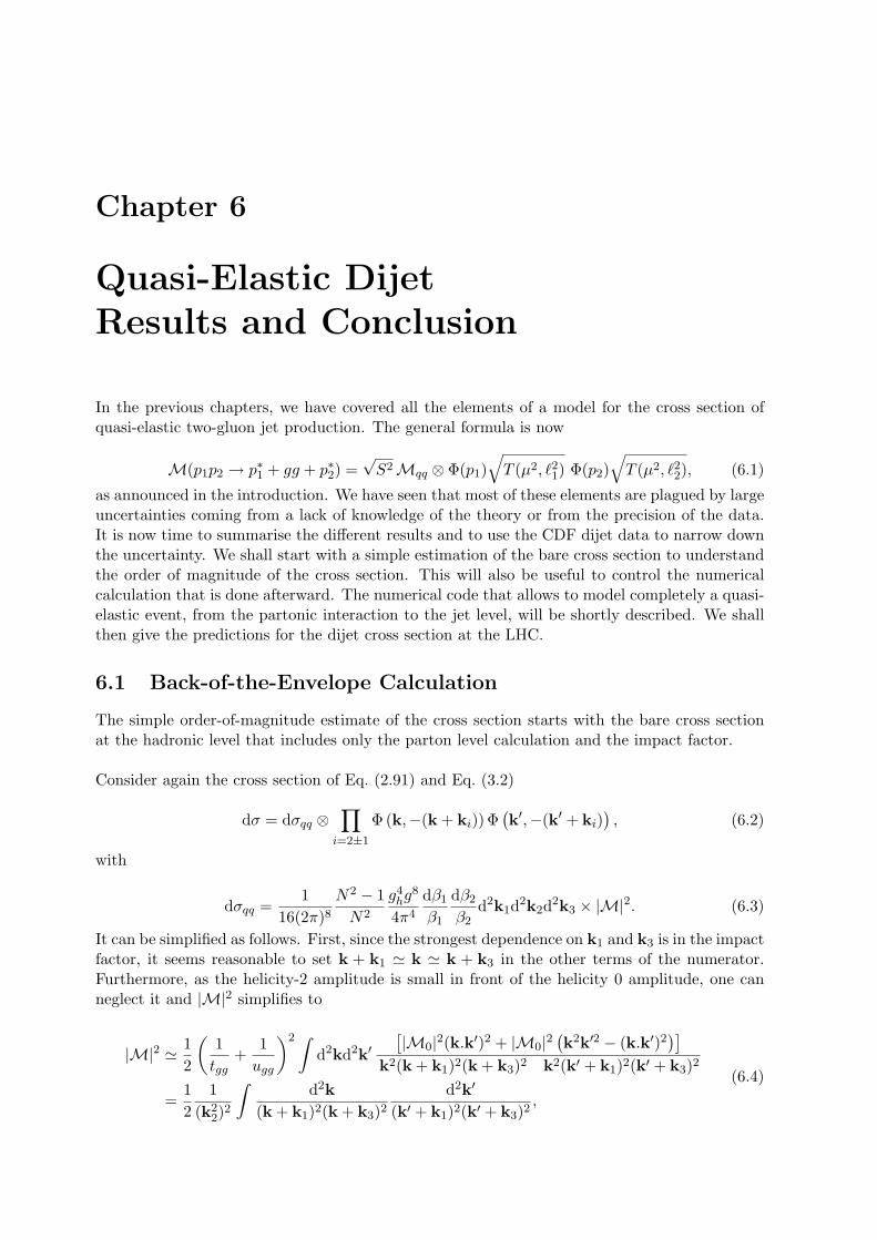
Chapter 6

Quasi-Elastic DijetResults and Conclusion

In the previous chapters, we have covered all the elements of a model for the cross section ofquasi-elastic two-gluon jet production. The general formula is now

M(p1p2 → p∗1 + gg + p∗2) =√S2Mqq ⊗ Φ(p1)

√T (µ2, `21) Φ(p2)

√T (µ2, `22), (6.1)

as announced in the introduction. We have seen that most of these elements are plagued by largeuncertainties coming from a lack of knowledge of the theory or from the precision of the data.It is now time to summarise the different results and to use the CDF dijet data to narrow downthe uncertainty. We shall start with a simple estimation of the bare cross section to understandthe order of magnitude of the cross section. This will also be useful to control the numericalcalculation that is done afterward. The numerical code that allows to model completely a quasi-elastic event, from the partonic interaction to the jet level, will be shortly described. We shallthen give the predictions for the dijet cross section at the LHC.

6.1 Back-of-the-Envelope Calculation

The simple order-of-magnitude estimate of the cross section starts with the bare cross sectionat the hadronic level that includes only the parton level calculation and the impact factor.

Consider again the cross section of Eq. (2.91) and Eq. (3.2)

dσ = dσqq ⊗∏i=2±1

Φ (k,−(k + ki)) Φ(k′,−(k′ + ki)

), (6.2)

with

dσqq =1

16(2π)8

N2 − 1N2

g4hg

8

4π4

dβ1

β1

dβ2

β2d2k1d2k2d2k3 × |M|2. (6.3)

It can be simplified as follows. First, since the strongest dependence on k1 and k3 is in the impactfactor, it seems reasonable to set k + k1 ' k ' k + k3 in the other terms of the numerator.Furthermore, as the helicity-2 amplitude is small in front of the helicity 0 amplitude, one canneglect it and |M|2 simplifies to

|M|2 ' 12

(1tgg

+1ugg

)2 ∫d2kd2k′

[|M0|2(k.k′)2 + |M0|2(k2k′2 − (k.k′)2

)]k2(k + k1)2(k + k3)2 k2(k′ + k1)2(k′ + k3)2

=12

1(k2

2)2

∫d2k

(k + k1)2(k + k3)2

d2k′

(k′ + k1)2(k′ + k3)2,

(6.4)

106 Results and Conclusion

as |M0|2 = 1 and

1tgg

+1ugg

=1k2

2

. (6.5)

Now, one can change notation and write the longitudinal phase space as a function of two newvariables

x ≡ β1

β2, x ∈ [1, xmax],

β ≡√β1β2, β ∈ [βmin, βmax],

(6.6)

where the domain of integration in x comes from the ordering β1 > β2. The change of variablegives

dxdβ =

∣∣∣∣∣∣∣1β2

− xβ2

β2β1

β2β2

∣∣∣∣∣∣∣ dβ1dβ2, (6.7)

where we used Eq. (6.6) and one has then

dxx

dββ

=dβ1

β1

dβ2

β2. (6.8)

The partonic cross section of Eq. (6.3) becomes

dσqq =1

8π6

N2 − 1N2

α2sα

4

(k22)2

dββ

dxx

d2k1d2k2d2k3

×∫

d2k(k + k1)2(k + k3)2

d2k′

(k′ + k1)2(k′ + k3)2,

(6.9)

using the definition of the coupling g2 = 4πα. The hadronic cross section is obtained aftermultiplication with the impact factors, one for each proton in the process:

dσ =1

8π6

(N2 − 1)N2

α2sα

4

(k22)2

dββ

dxx

d2k1d2k2d2k3

×∫

d2kΦ (k,−(k + k1)) Φ (−k, (k + k3))

(k + k1)2(k + k3)2d2k′

Φ (k′,−(k′ + k1)) Φ (−k′, (k′ + k3))(k′ + k1)2(k′ + k3)2

.

(6.10)

To make an estimate of this, the dimensionless quantity

〈Φ4〉 =1π4

∫d2k1d2k3

[∫d2k

Φ (k,−(k + k1)) Φ (−k, (k + k3))(k + k1)2(k + k3)2

]2

, (6.11)

is introduced and the expression simplifies to

dσ =1

8π2

(N2 − 1)N2

α2sα

4

∫dββ

dxx

∫d2k2

(k22)2〈Φ4〉. (6.12)

In the case of a simple impact factor that doesn’t depend on the longitudinal fraction of momen-tum, the longitudinal integral over x and β reduces to integration over the whole phase spaceand one has

6.1 Back-of-the-Envelope Calculation 107

dσ =1

8π6

(N2 − 1)N2

α2sα

4

∫ βmax

βmin

dββ

∫ xmax

1

dxx

∫d2k2

(k22)2〈Φ4〉

=1

8π6

(N2 − 1)N2

α2sα

4

[log(βmax

βmin

)log(xmax)

] ∫d2k2

(k22)2〈Φ4〉,

(6.13)

while the last integral over k22, if k2

2 > k22,min, is

∫d2k2

(k22)2

=∫ 2π

0

∫ s

k22,min

dθdk22

21

(k22)2

= −π1s

+ π1

k22,min

' π 1k2

2,min

,

(6.14)

in the large-s limit. Hence, the cross section becomes

dσ ' 19πα2sα

4 1k2

2,min

[log(βmax

βmin

)log(xmax)

]〈Φ4〉, (6.15)

and one needs to know the value of the different quantities. The limits on β and x are difficultto estimate in our kinematics but they can actually be extracted from their distributions in thenumerical calculation and one obtains

log(βmax

βmin

)log(xmax) ' O(30). (6.16)

Now, the next step is the evaluation of 〈Φ4〉, which is an intrinsically soft quantity but can berelated to the elastic cross section in the same approximation, that is

σel =4α4

81π2

∫d2k1

[∫d2k

k2(k + k1)2× Φ2(k,−(k + k1))

]2

. (6.17)

This expression is close to Eq. (6.11) and in particular, one can assume in both cases that thestrongest k1 dependence comes from the exponential factor

Φ ∝ e− 12B |t| f(k). (6.18)

Consequently, because here |t| = k21 and k2

1 is small, one has to compute

σel ' 4α4

81π2

∫d2k1

[∫d2kk4× e−Bk2

1Φ2(k,−k)]2

=2α4

81π2

π

B

[∫d2kk4

Φ2(k,−k)]2

=2α4

81πB

[∫d2kk4

Φ2(k,−k)]2

.

(6.19)

Similar approximations lead to


〈Φ4〉 ' 1π4

∫d2k1d2k3

[∫d2k

e−12Bk2

1Φ (k,−k) e−12Bk2

3Φ (−k,k)k2k2

]2

=1

π2B2

[∫d2kk4

Φ2(k,−k)]2

.

(6.20)

Hence, one has

α4〈Φ4〉 =81σel2πB

. (6.21)

The elastic cross section at TeVatron energy is 19.7 mb [138] and the corresponding protonslope B ∼ 4 GeV2 leads to

α4〈Φ4〉 ' O(60), (6.22)

that itself leads to an estimation for the quasi-elastic dijet cross section at the hadronic levelusing Eq. (6.15) which is now

dσ ' 9σel2π2B

α2s

1k2

2,min

[log(βmax

βmin

)log(xmax)

]. (6.23)

For |k2,min| = 10 GeV and α2s = 0.04, it gives roughly σ ' 10 µb.

By comparing this result with the CDF data for which the cross section is about 1 nb atEmin⊥ > 10 GeV, one can directly note that it is three order of magnitude beyond. This indicates

that the Sudakov suppression indeed plays a crucial role. In Sec. 4.2.3, we have estimated it tobe of the order of 8.10−3 in the double-log approximation. If one adds the shift in Emin

⊥ fromthe splash-out of Sec. 5.2 and the gap survival, it brings back our estimate of the cross sectionof about 10 nb in rough agreement with data.

6.2 Numerical Implementation

The calculation of the dijet quasi-elastic cross section cannot be done analytically if one wantsto include all the corrections and preserve the exact transverse kinematics. In particular, onehas to compute 11 different integrals. The choice was made to use a Monte-Carlo integrationthat is more or less the only way to perform this number of integrals in a finite time.

Hence, the integration over each variable is done by Vegas [139], a dedicated program for multi-dimensional integration. The idea behind the Monte-Carlo technique is to distribute randomlythe n integration variables between their limits and compute the integrand at each of theserandom points. After that, a sum over the weighted averages is computed and from iteration toiteration, the increments size for each variables is adjusted to concentrate in the region wherethe integrand is the largest. Hence, Vegas changes the density of points, and the weight of theintegrand, until the desired precision is reached. The main point is that the set of n pointsforms a distribution of the integration variables and if those variables are related to physicalquantities, i.e. components of the four-momenta, rapidity, etc, one is left with a fully-definedhigh-energy event at each step.The structure of the code is then simple, one starts with the parton-level calculation to whichone adds the corrections to compute the cross section. Each step of Vegas defines a completeset of four-momenta for the final particles and then the numerical calculation behaves exactly asan event generator with all its possible advantages. Firstly there is the possibility to apply the

6.3 Presentation of the Numerical Results 109

kinematical cuts of the CDF analysis to reproduce exactly the conditions of the measurementand consequently, to obtain a correct comparison between theory and data. Secondly, one canproduce distributions over several quantities and this is useful to test the accuracy of the resultas well as to control the numerical calculation. In addition, one has the possibility to interfacethe calculation with a hadronization code such as Pythia1, jet algorithms or a full detector-response simulation.

In one picture, the structure of the code is represented in Fig. 6.1.

+

Numerical Integration

Splash−Out

Hadronization

Jet− Cone Algorithm

Application of Experimental Cuts

Possibility to run Analysis and Detector Simulations→ Delphes

Exact TransverseKinematics

Higher−Order and SoftCorrections

Forw

ardP

hysicsM

onte−C

arlo:

FP

MC

Model

Monte− Carlo

Figure 6.1: Structure of the code. The whole framework is implemented in FPMC, aMonte-Carlo for forward physics under the name of the CHIDe model.

6.3 Presentation of the Numerical Results

Traveling across the previous chapters has already introduced some of the main results andcurves and, in particular, has demonstrated the sensitivity of the final answer to the differentparameters of the calculation. Here, we would like to summarise those results and show howit is possible to use the CDF data to narrow down the uncertainties. Because the data arean essential part of this study, we shall start with a short description that will be followed bythe presentation of our reference parametrisation and of the corresponding evaluation of theuncertainties.

1Note that in FPMC the hadronization is performed by HERWIG.


6.3.1 CDF Run II Data

Dijet quasi-elastic data were published in 2008 and are the result of 5 years of data tak-ing during the Run II of the TeVatron pp collider. The energy in the center-of-mass framewas√s = 1.96 TeV and events were collected by the upgraded CDF II detector [57].

Quasi-elastic events are selected by requesting the presence of at least two jets with transverseenergy Emin

⊥ > 10 GeV within the rapidity region |η| < 2.5. They are reconstructed withthe CDF Midpoint algorithm using a cone radius of 0.7 in the η/φ space and the transverseenergy E⊥ of the jet is defined as the sum of the Ei⊥ of the clustered calorimeter towers. Oneof the main difficulties is to extract the quasi-elastic signal from the other kinds of dijet pro-ductions, i.e. inclusive, single diffractive and non diffractive. The CDF detector only possessesRoman pot stations downstream in the antiproton direction and can only trigger final antipro-tons. So, the strategy developed for the analysis is to look at the dijet mass fraction distributionof the full data sample with

Rjj =Mjj

Mx, (6.24)

where Mjj is the mass of the dijet system and Mx the invariant mass of the sum of the four-momenta of all objects in the final state, proton and antiproton excluded. The idea is tomeasure the distribution and search for an excess of events at high Rjj , which exceeds the ex-pectation of the POMWIG Monte-Carlo simulation [140] of dijet production in double pomeronexchange (DPE), which in fact doesn’t simulate quasi-elastic processes. Obviously, the kind ofevent we are interested in is expected to have a mass fraction distribution peaked at large Rjjas the only two jets produced in the final state should carry, up to the splash-out correction,the total produced mass.From the complete sample of dijet produced in double-pomeron exchange, the event has to passa series of cuts that are chosen to enhance the quasi-elastic signal. There are four cuts, respec-tively on the transverse energy of the two jets, on their rapidity, on the size of the gap and onthe momentum lost by the antiproton tagged in Roman pots. The values of the different cutsare given in Table 6.1 and one should note that they are not symmetric as only the antiprotonlongitudinal loss of momentum is measured. In addition, a third jet veto is applied that allows

Parameter RangeEjet1,2⊥ > Emin

⊥|ηjet1,2| < 2.5|ηgap ' |ηp − ηjj| >3.6(α1 + α2) 0.03 < (α1 + α2) < 0.08

Eji>3⊥ < 5 GeV

Table 6.1: Experimental cuts for CDF Run II data [57].

the presence of extra jets only if their energies are smaller than 5 GeV. The outcome for the dijetmass distribution of [57] shows an excess of events compared to the POMWIG prediction. Thisexcess is well reproduced within the statistical uncertainties by the ExHume Monte-Carlo forquasi-elastic dijet production. POMWIG populates the low-Rjj region and ExHume events areat large Rjj , but this second distribution exhibits a long tail extending toward small-Rjj valuesdue to gluon radiation. The issue is that one has to trust the Monte-Carlo simulation in orderto extract the quasi-elastic data in the region of small dijet mass fraction and it introduces someuncertainties on the result. The CDF collaboration exploits the fact that the rapidity distribu-


tion of inclusive dijet events is more symmetric around ηjet1,2 = 0 than the quasi-elastic one.Moreover, the cut on α introduces an asymmetry in the collision and boosts the dijet systemtoward negative rapidity values for quasi-elastic events only. These kinematical properties wereused to improve the analysis. One can show the origin of this effect starting with the definitionof the longitudinal momentum lost by the antiproton (α1+α2), that in the kinematics of Chap. 2is calculated from

α1 =(k1 − k2)2

β1s, α2 =

(k2 − k3)2

β2s, (6.25)

and gives

α1 + α2 =β2(k1 − k2)2 + β1(k2 − k3)2

β2β1s

' (β2 + β1)k22

β2β1s

' sgg(β1 + β2)s

,

(6.26)

using Eq. (2.76). One can evaluate the maximum and minimum of the longitudinal momentumlost by the proton (β1 + β2) assuming that sgg ' 4E2

min,⊥ at the TeVatron energy of√s =

1960 GeV, to get

(β1 + β2)max ' sggs

1(α1 + α2)max

' 0.0012. (6.27)

Given the bounds of Table 6.1 one has (β1 +β2) < (α1 +α2) and the rapidity of the dijet system

ηjj =12

log(β1 + β2

α1 + α2

), (6.28)

is negative. The data were then divided in the data sample A, for which at least one of the twoleading jets has ηjet1,2 < −0.5 and contains most of the quasi-elastic events while data sample Bwith ηjet1,2 > −0.5 includes predominantly background.

We have shown the result of the CDF analysis in Fig. 1.12. We shall now tune the differentparameters of our model to reproduce it. In order to compare the same quantities, we appliedthe same cuts as those of Table 6.1 and the accuracy of the result can be tested by producingsome of the distributions shown in the CDF paper.

6.3.2 Choice of Parametrisation

Using those CDF measurements, one can choose among the different parametrisations of thedijet quasi-elastic cross section, one that gives a curve going through the data points. We stressthat it is not a prediction but only an accurate parametrisation. From this particular curve, onecan now study the effect of a change in the parametrisation and evaluate the theoretical uncer-tainties that affect the calculation. In addition, the reference parametrisation is the basis usedto extrapolate our result to LHC energies or to predict the Higgs boson quasi-elastic cross section.

The available parameters come in the impact factor, the Sudakov form factor, the gap survivaland the splash-out. Each ingredient was described in details and some prescriptions were ruledout either for theoretical reasons or for total incompatibility with the data. Consequently, thefree parameters left are


• Impact factor: Type of the ΦUgD, i.e. Fit: 1, 2, 3 or 4,

• Sudakov Form factor: Upper limit µ, Lower limit `,

• Gap survival: 〈S2〉 between 5% and 15%,

• Splash-out: Three different prescriptions.

The complete parametrisation of the reference curve shown in Fig. 1.12 is given in Table 6.2 andis obtained after the application of the restrictions of Table 6.1. Without cuts, one has the curve

Parameter Value Reference- GeneralΛQCD 0.20 GeV- Impact factorΦUgD Fit-4 Sec. 3.3- Sudakov form factorExponentiation log2 + log+constant Sec. 4.2.2∆ |q|/µ angular ordering in Sec. 4.1Coupling constant Running with k2

2

Upper scale µ2 = 2k22 Sec. 4.2.1

Lower scale `2 = 2(k + ki)2 Sec. 4.2.1- Gap-Survival Probability〈S2〉 15% Sec. 5.1- Splash-OutEjet⊥ 0.75Eparton

⊥ Sec. 5.2

Table 6.2: Parameters of the reference curve of Fig. 1.12.

of Fig. 6.2.a that is about 3.5 times bigger. Using FPMC2, one can study more precisely the

Without CutsCDF data

Emin⊥ [GeV]

σ[n

b]

403530252015105

1000

100

10

1

0.1

0.01

0.001

0.0001

(a)

Third jet vetoOnly two jets

CDF data

Emin⊥ [GeV]

σ[n

b]

403530252015105

10

1

0.1

0.01

0.001

0.0001

(b)

Figure 6.2: The effect of CDF kinematical cuts. (a) The plain curve is again thereference and the higher curve is obtained by removing all cuts. (b) Theeffect of allowing only two leading jets in the final state or any number ofadditional jets if Ejeti>3

⊥ < 5 GeV. This last plot was obtained using FPMCwith exactly the same parameters as for the reference curve.


effect of the experimental analysis and in particular of the third jet veto. In Fig. 6.2.b, one cannote the importance of this additional constraint as the two curves show the difference betweenrestricting the analysis to two jets or allowing for any number of extra jets with Ejeti>3

⊥ < 5 GeV.This veto changes the cross section by a factor 0.8 and the application of the cone algorithmsmoothes the curvature.

The question of other distributions is interesting as we can check the coherence of the model withthe data. As an example, Fig. 6.3 shows two distributions similar to those of the CDF paper,

(a)

3.6 < |ηgap| < 5.9

E⊥ > 10 GeV

η∗ = (ηjet1 + ηjet2)/2

dσ/d

η∗

[nb]

3210-1-2-3

1

0.8

0.6

0.4

0.2

0

(b)

Figure 6.3: (a) Dijet mass fraction. (b) Mean jets rapidity distribution.

namely the Rjj distribution and the mean jet-rapidity distribution. One can also have a lookat the assumption of negative rapidity for the dijet system due to cuts used, and beside one cancheck the effect of the choice of the scale in the Sudakov form factor on this assumption. In theanalysis, the rapidity space was divided into four regions, shown in Fig. 6.4, depending on therapidity of the leading and second jet. According to ExHume, the region where both ηj1 and ηj2are smaller than -0.5 is dominated by the quasi-elastic signal while the region with ηj1, ηj2 < −0.5contains few quasi-elastic events. One can evaluate the cross section in each of the four regionsand compute the ratio between the two. For the reference parametrisation and Emin

⊥ >10 GeV,one has

RBRA

= 0.65. (6.29)

Here, let us remind the reader that the upper scale of the Sudakov form factor is 2k22 whereas

in ExHume it is µ = 0.62√sgg. In fact, using this very scale in our calculation together withparameters that fit the data, we obtain

RBRA

∣∣∣∣∣µ=0.62

√sgg

= 0.45, (6.30)

that is slighty different. Once again here, a more detail data analysis of this particularity andnew results from LHC should help to settle the issue of the Sudakov form factor upper limit.The choice made for the parametrisation of the reference curve is not unique and one could have

2The parton-level calculation in FPMC is identical to the parton-level calculation in the code used for thethesis so that the two results are in agreement to better than 1%. The small difference is from the method ofintegration as one uses VEGAS while FPMC uses a traditional Monte-Carlo integration with a smaller precision.


−3

3

3

0

0

−0.5

−0.5

Leading jet rapidity

Sec

ond

jet

rapid

ity

ηj1 < −0.5

ηj2 < −0.5

Sample A

Sample B

ηj1 > −0.5

ηj2 > −0.5

Figure 6.4: Division of the rapidity space in four different regions depending on therapidity of the leading and second jet. According to ExHume, the regionwhere both ηj1 and ηj2 are smaller than -0.5 is dominated by the quasi-elastic signal while the region with ηj1, ηj2 > −0.5 contains few quasi-elastic events.

found another set of parameters that gives a curve in agreement with the data. By changingonly the type of ΦUgD, µ, ` and 〈S2〉, it is possible to obtain the curves of Fig. 6.5 that are

Ref 3Ref 2

Emin⊥ [GeV]

σ[n

b]

403530252015105

100

10

1

0.1

0.01

0.001

0.0001

Figure 6.5: Two different sets of parameters that also give a curve in agreementwith the data. The corresponding parametrisations can be found in Ap-pendix B.5.

similar to the reference curve. One will see what happens to these curves after the extrapolationto LHC but we first summarise the uncertainties.

6.4 Extrapolation to the LHC 115

6.3.3 Uncertainties

The full uncertainty, based on the reasonable theoretical choices described in this thesis, is shownin Fig. 6.6.a. Restricting the model with the TeVatron data considerably reduces the uncertainty

403530252015105

100

10

1

0.1

0.01

0.001

0.0001

1e-05

CDF data

Emin⊥ [GeV]

σ[n

b]

(a)

403530252015105

100

10

1

0.1

0.01

0.001

0.0001

CDF dataCentral Values

CDF Uncertainties

Emin⊥ [GeV]

σ[n

b]

(b)

Figure 6.6: (a) Several reasonable parametrisations of ingredients for dijet quasi-elastic calculation and the resulting estimations of the cross section.(b) Restriction of the model using the TeVatron data. The differentparametrisations are given in Appendix B.5.

and one is left with the band of Fig. 6.6.b that is still affected by an uncertainty of 2 order ofmagnitude at high transverse energy.

Due to the choice of the intrinsic parameters, each ingredient of the calculation can change thefinal result, and those factors are summarised:

Ingredient UncertaintyImpact Factor 3Sudakov form factor 10Gap survival 3Splash-out 1.5

Three remarks are in order and underline the fact that the evaluation of the total error isambiguous. Firstly, a change in one parameter can be compensated by a change in another.Secondly, the sensitivity depends on the considered parameter, for instance the calculationis particularly sensitive to the parametrisation of the Sudakov form factor but only in thelow-energy region. Taking that into account, we don’t want to give a number that could bemisinterpreted and conclude this section by saying that the uncertainty on the dijet quasi-elasticcalculation is large.

6.4 Extrapolation to the LHC

The formulae derived for the dijet quasi-elastic cross section can be equally used to estimate thedijet cross section at the LHC.

The obvious change from the TeVatron to the LHC comes from the kinematical cuts as LHCdetectors are different from those of the TeVatron. In particular, LHC detectors may have a bet-ter forward instrumentation, with the addition of the very forward detectors RP220 and FP420


in ATLAS and CMS, one might have the largest rapidity coverage ever. Specific cuts will beused to search for diffractive events and they are given in Table 6.3, assuming the presence of

Parameter Range|ηjet1,2| < 1(α1 + α2) 0.002 < (α1 + α2) < 0.2(β1 + β2) 0.002 < (β1 + β2) < 0.2

Table 6.3: Experimental cuts [72] for the LHC multi-purpose detectors ATLAS andCMS including the very forward detectors RP220 and FP420.

both RP220 and FP420. Note that without them, quasi-elastic events cannot be measured byproton tagging as final protons are outside the rapidity coverage of the central detector.One also has to extrapolate the proton impact factor to LHC energies where the emitted gluonswould have a smaller longitudinal fraction of momentum, which is easy as the impact factor builtin Chap. 3 already includes a dependence in the center-of-mass frame energy. There is also thequestion of the gap-survival probability for which the extrapolation to LHC is model-dependent.For this estimate, we have decided to use the prescription

〈S2〉∣∣∣LHC

=12〈S2〉

∣∣∣TeVatron

. (6.31)

Note that this is just an assumption, in agreement with [122].Our prediction for the dijet quasi-elastic cross section at LHC is shown in Fig. 6.7 for an energyin the center-of-mass frame of 10 TeV with and without cuts. We show the 10 TeV curves

12010080604020

1000

100

10

1

0.1

0.01

Central ValuesCDF Uncertainties

Emin⊥ [GeV]

σ[p

b]

(a)

12010080604020

1000

100

10

1

0.1

0.01


Emin⊥ [GeV]

σ[p

b]

(b)

Figure 6.7: (a) Dijet quasi-elastic cross section at the 10 TeV. The inner band corre-sponds to curves that reproduce the central values of the CDF data butslightly diverge at LHC energies, the outer band corresponds to the 1σ er-rors. (b) Same but without cuts.

because due to technical issues the LHC shouldn’t reach 14 TeV before 2012. We neverthelessgive the prediction for

√s=14 TeV and

√s=7 TeV with cuts in Fig. 6.8.

6.4 Extrapolation to the LHC 117

1009080706050403020

1000

100

10

1

0.1

0.01


Emin⊥ [GeV]

σ[p

b]

(a)

12010080604020

1000

100

10

1

0.1

0.01


Emin⊥ [GeV]

σ[p

b]

(b)

Figure 6.8: (a) Dijet quasi-elastic cross section at the 7 TeV and (b) dijet quasi-elasticcross section at the LHC (14 TeV). Both curves are obtained after the cutsof Table 6.3.

The results for the LHC tuned to the CDF data are unavoidably plagued by the same largeuncertainties as those of the TeVatron and their range is indicated by the outer band. Theinner band shows how different sets of parameters, tuned on the TeVatron data to reproducethe central values, diverge after extrapolation to the LHC. As for the TeVatron, one can checkthe importance of the non-perturbative region and the conclusion is confirmed that the gluonloop is still dominated by the soft region as shown in Table 6.4. One can also note an interesting

Experiment EminT σpert/σ

LHC 14 TeV 50 GeV 55%LHC 7 TeV 50 GeV 30%LHC 10 TeV 50 GeV 45%LHC 10 TeV 100 GeV 30%

Table 6.4: Ratio σpert/σ where σpert is the value of the cross section if all gluon trans-verse momenta are larger than 1 GeV. Different experiments and jet trans-verse minimum energies are presented but in all cases the parametrizationis the one of the reference curve.

feature of the calculation that makes the uncertainty on the upper limit in the Sudakov formfactor vanish at large s and high Emin

⊥ . Fig. 6.9 illustrates the dominance of the Sudakov formfactor double logs at large Emin

⊥ .So, the data constrain the uncertainty at the LHC and allow for a better prediction of thequasi-elastic dijet cross section. However, the cross section presents the same characteristic asat the TeVatron, namely, a calculation dominated by the non-perturbative region and largeuncertainties.


µ2/2µ2 = 2k2

2

2µ2

Emin⊥ [GeV]

σ[p

b]

1009080706050403020

1000

100

10

1

0.1

Figure 6.9: Results at the LHC for three different values of the upper limit in theSudakov form factor: at large s and high Emin

⊥ the uncertainty vanishes.

6.5 Conclusion

Our work was dedicated to the calculation of the dijet quasi-elastic cross section and to theevaluation of the theoretical uncertainties. We have described all the ingredients going intothe calculation. In particular, we have kept an exact transverse kinematics and paid specialattention to the higher-order corrections embodied by the introduction of the Sudakov formfactor. We have shown that the result is plagued by large uncertainties that can be reducedusing the recent CDF data.The extrapolation to the LHC, for different possible energies, shows that the cross section is ofthe order of 2 pb at

√s=10 TeV for jets of minimum transverse energy 50 GeV. Under the present

assumptions, one then can be confident in the fact that quasi-elastic dijet should be seen. Notehowever that in the worst-case scenario, the gap survival is zero and quasi-elastic cross sectionsvanish, destroying in the same time the hope for all other high-mass quasi-elastic processes.Early dijet measurements at LHC are then crucial and the first data will give information ongap survival. If the cross section survives, then new measurements will help to narrow down theuncertainty.

Part II

Higgs Boson Quasi-ElasticProduction

“How doth the little crocodileImprove his shining tail,

And pour the waters of the NileOn very golden scale!

How cheerfully he seems to grin,How neatly spread his claws,And welcome little fishes inWith gently smiling jaws!”


One of the interesting features of quasi-elastic production is that the structure of the calculationremains the same in all kinds of production. Consequently, the main idea of the thesis is to keepthe parametrisations tuned to the CDF dijet data to predict the Higgs boson quasi-elastic crosssection at the LHC. This choice is not innocent as the Higgs boson is the last particle of theStandard Model not yet detected experimentally, and without it, the theory is not complete.One can then guess that the Higgs boson hunt is one of the most exciting questions today.Up to now, the Higgs boson has escaped all its hunters although at LEP during the last runs,physicists have thought they had observed a signal for it but they had to make space for thebuilding of LHC before any convincing evidence. A new machine is now ready to resume thesearch but, with the tremendous energy available, the Higgs boson signature may remain com-pletely hidden in the background of old and new processes for a long time, and this is wherequasi-elastic production may matter.

Quasi-elastic cross sections for the production of the Higgs boson or any other heavy particlesare small. Nevertheless, those events have two very clear signatures, the rapidity gap and theremaining protons in the final state. Besides, with the appropriate detectors, it will be possibleto reconstruct the mass of the centrally-produced system from the measurement of the miss-ing mass of the final protons. Consequently, the clean signature is the key point that makesquasi-elastic production a competitive discovery channel at LHC energies. From the theoreticalpoint of view, the situation is complicated as large uncertainties affect the calculation and thesoft physics that enters the process is not fully under theoretical control. However, we havedetermined a set of parametrisations that reproduces the CDF data. Using the fact that thetopology of the dijet diagram, shown schematically in Fig. 6.10.a, is the same as that of the

(a)

H

(b)

Figure 6.10: Topology of the quasi-elastic production for (a) dijet and (b) Higgs boson.Apart from the hard subprocess, the topology is identical, so that thesoft pieces.

Higgs diagram shown in Fig. 6.10.b, these parametrisations can be used to predict the Higgsboson production cross section.

In the first chapter, we shall briefly review the Higgs boson modes of production and present

124

the Durham model which is the model closest to ours. In the second chapter, we discussthe calculation in the quasi-elastic regime but we focus only on the differences from the dijetcalculation and on the effect of the parametrisation choices as the main ingredients were alreadydescribed. Finally, we shall give a prediction for the Higgs boson quasi-elastic cross section atthe LHC.

Chapter 7

Searching for the Higgs Boson

The search of the Higgs boson is an old quest but the idea of using the quasi-elastic channelfor its discovery appeared 20 years ago [141]. It is now ready to be tested at the LHC usingthe current knowledge of the theoretical calculation and the possibility to use very forwarddetectors. Moreover, this kind of production is usually viewed as a golden channel due to theclear signature of the events. So, we show here why quasi-elastic Higgs boson production canbe attractive from the experimental point of view.

7.1 Overview

At the LHC, the two dominant channels should be gluon and vector-boson fusion. In both cases,the final state is complicated and requests a careful analysis of the event in addition with powerfulmethods to tag the Higgs boson decay products to reconstruct its mass. Following [142, 143],we give here a brief summary of different inclusive cross sections and of their uncertainties.

7.1.1 Higgs-Boson Production in the Standard Model

The number of Higgs boson production mechanisms in the SM that lead to a sizable cross sectionand detectable final states is quite small. One has the production by gluon-gluon fusion [144],by WW and ZZ fusion [145], by associated production with W and Z bosons [146, 147], byassociated production with tt [148–151] and representative Feynman diagrams are shown inFig. 7.1.

t

t

t

t

t

W (Z)

W (Z)

W (Z)

H H

H

H

H

(a) (b) (c)

(d)

Figure 7.1: Representative diagrams of the main Higgs boson production mechanisms.(a) Gluon-gluon fusion, (b) vector boson fusion, (c) associated productionwith W and Z and (d) associated production with top pair quarks.

126 Searching for the Higgs Boson

The corresponding cross sections as functions of the Higgs boson mass at√s=10 TeV are shown

in Fig. 7.2 and one can directly note that gluon fusion is largely dominant in the whole considered

qq → ZHqq′ → WH

qq → qqH

gg, qq → ttH

gg → H

mH [GeV]

σ[p

b]

200180160140120100806040

100

10

1

0.1

0.01

Figure 7.2: Total cross section for different production mechanisms at LHC 10 TeV.Adapted from [143].

mass range. The estimates for inclusive Higgs-boson cross sections at the LHC are from 10 pbup to 100 pb in the intermediate mass region for all modes of production combined and themain uncertainty is the knowledge of the gluon distribution at small x. According to [143], it isevaluated to be ±20% and the other source of error is the values of several input parameters asfor example the top mass. Fortunately, corrections are now known for most of the processes andthe parameters start to be more and more constrained due to precision measurements from LEP,the TeVatron and other experiments1.The question to address is the possibility to reconstruct the Higgs boson from the particles ob-served in the detector. Actually, if one considers the LEP results [152] and the recent TeVatrondata [153] that constrain the mass, the SM Higgs boson should have a mass beyond 114 GeV ac-cording to LEP and the TeVatron data excluded the mass region between 160 GeV and 170 GeVat the 95% confidence level2. Moreover, the few Higgs boson candidates observed at the endof the last run of the LEP collider [154] points to a light Higgs boson. In this case, as shownin Fig. 7.3 that presents the branching ratio of the SM Higgs boson as a function of its mass,the main decay channel is a pair of heavy quarks, bb and the observation of the resonance re-quests a good mass resolution in addition to a technique of flavour identification for the finaljets. The background, constituted by processes with two b-jets in the final state is not small andaccording to reference [72], the signal-over-background ratio makes the dominant Higgs bosondecay products almost invisible. In this domain of mass, it is hence easier to deal with associ-ated productions that allow to trigger on the leptonic decay mode of the W or to look for raredecays, i.e purely leptonic or photonic final states, that have smaller branching fractions butrecognizable signatures allowing for excellent mass resolution. All these scenarios were studiedin great details by the LHC experiments and one should find in their technical reports [155, 156]the expectations as well as the evaluation of background not discussed here.

1A complete review of these as well as other processes in the Standard Model and beyond, can be foundin [142].

2The region between 155 GeV and 180 GeV is also excluded but only at 65% confidence level.

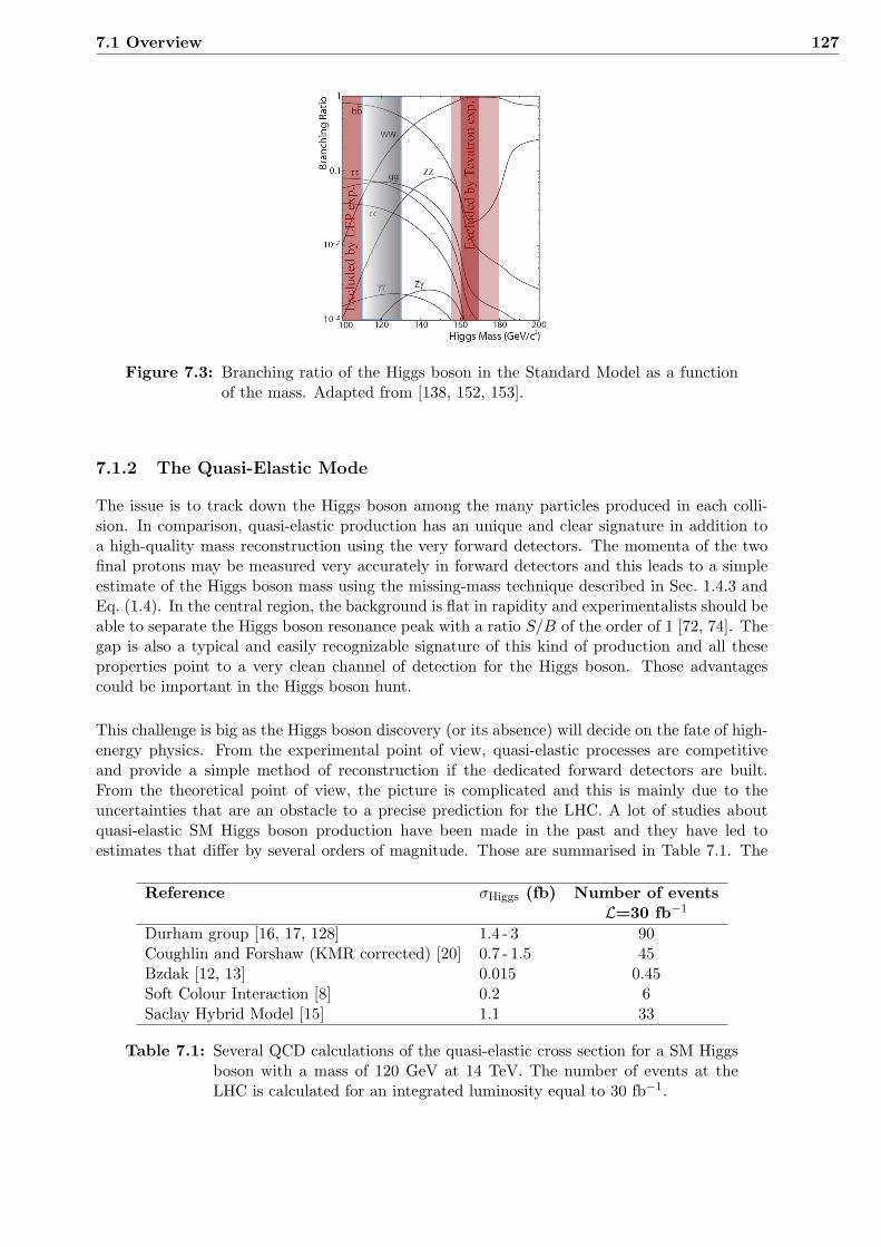
7.1 Overview 127

Figure 7.3: Branching ratio of the Higgs boson in the Standard Model as a functionof the mass. Adapted from [138, 152, 153].

7.1.2 The Quasi-Elastic Mode

The issue is to track down the Higgs boson among the many particles produced in each colli-sion. In comparison, quasi-elastic production has an unique and clear signature in addition toa high-quality mass reconstruction using the very forward detectors. The momenta of the twofinal protons may be measured very accurately in forward detectors and this leads to a simpleestimate of the Higgs boson mass using the missing-mass technique described in Sec. 1.4.3 andEq. (1.4). In the central region, the background is flat in rapidity and experimentalists should beable to separate the Higgs boson resonance peak with a ratio S/B of the order of 1 [72, 74]. Thegap is also a typical and easily recognizable signature of this kind of production and all theseproperties point to a very clean channel of detection for the Higgs boson. Those advantagescould be important in the Higgs boson hunt.

This challenge is big as the Higgs boson discovery (or its absence) will decide on the fate of high-energy physics. From the experimental point of view, quasi-elastic processes are competitiveand provide a simple method of reconstruction if the dedicated forward detectors are built.From the theoretical point of view, the picture is complicated and this is mainly due to theuncertainties that are an obstacle to a precise prediction for the LHC. A lot of studies aboutquasi-elastic SM Higgs boson production have been made in the past and they have led toestimates that differ by several orders of magnitude. Those are summarised in Table 7.1. The

Reference σHiggs (fb) Number of eventsL=30 fb−1

Durham group [16, 17, 128] 1.4 - 3 90Coughlin and Forshaw (KMR corrected) [20] 0.7 - 1.5 45Bzdak [12, 13] 0.015 0.45Soft Colour Interaction [8] 0.2 6Saclay Hybrid Model [15] 1.1 33

Table 7.1: Several QCD calculations of the quasi-elastic cross section for a SM Higgsboson with a mass of 120 GeV at 14 TeV. The number of events at theLHC is calculated for an integrated luminosity equal to 30 fb−1.

128 Searching for the Higgs Boson

KMR model [16, 17, 128] from Durham is described in the next section while the Coughlinand Forshaw model [20] differs only by the limits used in the Sudakov form factor. The modelused by Bzdak [12, 13] is based on the model for Higgs and dijet production by Bialas andLandshoff [84]. It includes the exchange of a pair of non-perturbative gluons, a dependence onthe energy and the momentum transfer as well as a Sudakov form factor that gives the exclusivecharacter of the process. After normalisation to the central inclusive production of dijet atthe TeVatron, this model is consistent with the CDF data for double diffractive exclusive dijetproduction3. The soft colour interaction [8, 157] model is a Monte-Carlo method implementedin Pythia that allows additional soft interactions between the partons produced in the hardprocess or between the partons and the proton colour field. These interactions only changethe colour configuration and lead to different hadronic final states. This is implemented bythe introduction of a new parameter that accounts for the unknown non-perturbative dynamicsphenomenologically determined from DIS data at the HERA collider. The particularity of thismodel is that it describes in the same framework diffractive and non-diffractive events wherethe formers are selected by the presence of a rapidity gap and a leading (anti)proton. The softcolour model is known to reproduce correctly the ratio of diffractive to non-diffractive events atthe TeVatron, however, the value of the cross section is strongly sensitive to details in the modeland in Pythia. Finally, the Saclay hybrid model is an exclusive model based on the exchange ofan hybrid pomeron defined by a combination of one hard and one soft color exchange, the formof the soft and hard parts are fixed by the corresponding data or suitable parametrisations.Note that this model doesn’t include a proper description of the impact factor, so that thenormalisation is not fixed by the model. Nevertheless, it reproduces correctly the slope andproperties of the dijet data.

7.2 The Durham Model

After the publication of the CDF dijet cross section, one model stayed, the one of Khoze, Martinand Ryskin or KMR model. We describe here its main lines, referring the reader to [16, 17, 158].

The cross section of the process represented schematically in Fig. 7.4, is assumed to factorize

x2

fg(x, x1,k2, µ2)

k

x x1

x

k

k

fg(x, x2,k2, µ2)

Figure 7.4: Schematic representation of the Higgs boson quasi-elastic amplitude.

between the effective luminosity L and the hard subprocess σ, with

σ = Lσ, (7.1)

and in particular3One should note that in 2005 the CDF Run II data weren’t published.

7.2 The Durham Model 129

∂σ

∂s∂y∂P2∂Q2= S2e−B(P2+Q2) ∂L

∂s∂ydσ (gg → H) . (7.2)

The different variables are the energy in the center-of-mass frame√s, the rapidity of the cen-

trally produced system y and the transverse momenta of the final protons P and Q. One canalso recognise in turn the gap-survival probability S2 and the logarithmic t-slope of the crosssection B = 4 GeV2, added by hand assuming that the dependence of the hard amplitude onfinal protons transverse momenta is small. The partonic cross section σ corresponds to theamplitude

M(gg → H) =12

1N2 − 1

∑a,b

∑λ1,λ2

δabδλ1,λ2Mλ1,λ2

ab (gg → H). (7.3)

The cross section to single-log accuracy is multiplied by a K factor of the order of 1.5, assumedto take into account next-to-leading-order corrections. The effective luminosity is given by

∂L∂s∂y

=(

π

(N2c − 1)

∫dk2

k4fg(x, x1,k2, µ2

)fg(x, x2,k2, µ2

))2

. (7.4)

The function fg stands for the unintegrated skewed gluon density related to the conventionalintegrated gluon distribution function and taken here in the simplified form [117]

fg(x, x1,k2, µ2

)= Rg

∂

∂ log k2

[√T (k, µ)xg(x,k2)

]. (7.5)

The factor Rg accounts for the skeweness4 and is found to be about 1.2 at the LHC energyof 14 TeV. One can note that the Sudakov form factor T (k, µ)

T (k, µ) = exp

[−∫ µ2

k2

dq2

q2

αs(q2)

2π

∫ 1−∆

0

(zPgg +

∑q

Pqg(z)

)dz

], (7.6)

with q and z the transverse and longitudinal components of the additional emission, is hereincluded in the differentiation. According to their next-to-leading order calculation [16, 17], theDurham group uses

∆ =q

q + µ,

µ = 0.62mH .(7.7)

The definition of these two scales will be discussed below, following a recent re-evaluation byCoughlin and Forshaw [20]. In this model, it is the presence of the Sudakov form factor thatmakes the integration infra-red stable and it is claimed that consequently, perturbative QCD isapplicable.

The Durham model has been developed for years and was the first to gather all the ingredientsneeded to reproduce the CDF data. It is one of the most complete models as it has been usedto predict different types of quasi-elastic productions, from Higgs boson, dijet, γγ, quark dijet,χc, . . . to supersymmetric particles, and as it gives results in agreement with the available data.It also investigates several aspects of the QCD calculation. One can note that our model issimilar to the Durham model but differs from it in several ways presented in the following.

4The fact that x 6= x1, g(x,k2) is the gluon density x = x1.

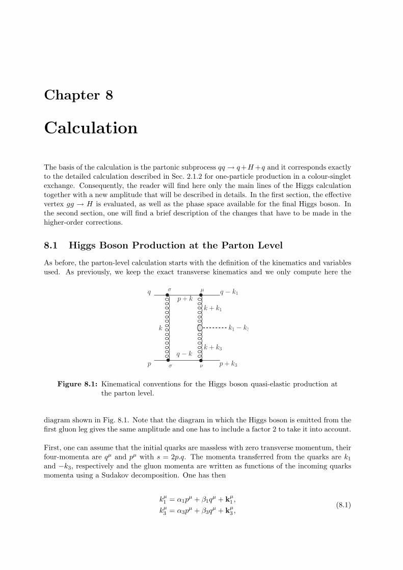
Chapter 8

Calculation

The basis of the calculation is the partonic subprocess qq → q+H+q and it corresponds exactlyto the detailed calculation described in Sec. 2.1.2 for one-particle production in a colour-singletexchange. Consequently, the reader will find here only the main lines of the Higgs calculationtogether with a new amplitude that will be described in details. In the first section, the effectivevertex gg → H is evaluated, as well as the phase space available for the final Higgs boson. Inthe second section, one will find a brief description of the changes that have to be made in thehigher-order corrections.

8.1 Higgs Boson Production at the Parton Level

As before, the parton-level calculation starts with the definition of the kinematics and variablesused. As previously, we keep the exact transverse kinematics and we only compute here the

q − k1

k1 − k3

q

p p + k3

k

k + k1

k + k3

p + k

q − k

σ

σ

µ

ν

Figure 8.1: Kinematical conventions for the Higgs boson quasi-elastic production atthe parton level.

diagram shown in Fig. 8.1. Note that the diagram in which the Higgs boson is emitted from thefirst gluon leg gives the same amplitude and one has to include a factor 2 to take it into account.

First, one can assume that the initial quarks are massless with zero transverse momentum, theirfour-momenta are qµ and pµ with s = 2p.q. The momenta transferred from the quarks are k1

and −k3, respectively and the gluon momenta are written as functions of the incoming quarksmomenta using a Sudakov decomposition. One has then

kµ1 = α1pµ + β1q

µ + kµ1 ,


µ + kµ3 ,(8.1)

132 Calculation

where all transverse vectors are denoted in bold. The produced Higgs boson momentum is

kµH = (α1 − α3)pµ + (β1 − β3)qµ + (k1 − k3)µ. (8.2)

In this description, the dominant kinematical region is where longitudinal components obey

1� αi, βi � |k2i |s

i = 1± 3, (8.3)

that corresponds to the quasi-elastic regime, with small momenta transferred from the initialparticles. At lowest order, the amplitude reads

M = g4C

∫d2k

Nµν

(k + k1)2(k + k3)2k2×M(gg → H), (8.4)

where g is the coupling constant between quarks and gluons, C=2/9 is the colour factor for thetwo-gluon exchange and M(gg → H) = Vµν is the gg → H effective vertex. One can use themethod developed in Sec. 2.1.2 to compute the longitudinal part of the integral and obtain

M = g4 C

2(2π)2s

∫d2k

1(k + k1)2(k + k3)2k2

×NµνVµν . (8.5)

Now, the next difficulty is to evaluate the contraction of the vertex with the numerator and onefirst needs an expression for the effective vertex.

8.1.1 Higgs Boson Effective Vertex

In the Higgs case, the hard subprocess is the collision of two gluons that produce the Higgsboson via a triangle of quarks and it can be obtained by calculating the sum of the diagramsshown in Fig. 8.2. In the Standard Model, the coupling between the Higgs boson and quarks is

+

t

=

Figure 8.2: The gluon-gluon to Higgs boson hard subprocess. Because the coupling ofthe Higgs boson to quarks is proportional to their masses, the top quarkcontribution dominates.

proportional to the mass of the quarks so that the top contribution dominates and is the onlyone taken into account. The exact calculation was made in [14] and shows that the effectivevertex can be written

Vµν = δab [(k + k1).(k + k3)gµν − (k + k1)ν(k + k3)µ]W1

m2H

+[(k + k1)2(k + k3)2gµν + (k + k1)µ(k + k3)ν(k + k1).(k + k3)

−(k + k1)µ(k + k1)ν(k + k3)2 − (k + k3)µ(k + k3)ν(k + k1)2] W2

m4H

,

(8.6)

where

W1 =(√

2Gf )1/2g2m2H

12π2N1, W2 =

(√

2Gf )1/2g2m2H

12π2N2. (8.7)

8.1 Higgs Boson Production at the Parton Level 133

Expressions for N1 and N2 come from the integration over the top loop in the specific kinematicsof production within a rapidity gap, i.e. (k + k1)2, (k + k3)2 � m2

H . Denoting a ≡ m2H/m

2t , one

has

N1 =6a

[1 +

(1− 4

a

)arctan2

(√a

4− a)]

. (8.8)

The calculation also demonstrates that the contribution of the W2 term can be neglected. Thiscomes from the fact that its tensor structure only gives contributions proportional to (k + ki)2

that are small in the considered kinematical regime. In addition, it was shown that |N2|2 isalways 30% smaller than the |N1|2 for a Higgs boson mass below 1 TeV and consequently, thiscorrection is negligible in front of the first term. This assumption will be discussed below andin Appendix C.1.

Using the Eikonal approximation and the indices as in Fig. 8.1, one can replace the upper (resp. lower)line of the diagram by 2pµpσ (resp. 2qσqν). The method [78] is valid whenever the gauge particleis soft and corresponds to taking the trace at the cross section level. Indeed, it can be shown,following the notation of Fig. 8.3, and computing the trace along the upper line, that is

q q + k′q − k1q + k q

p p − k p − k′p + k3 p

µ

ν

µ′

ν ′

σ

σ

σ′

σ′

Figure 8.3: Square of the diagram contributing to the Higgs boson production withall momenta and indices.

Tr U = Tr(q/γσ

′(q/+ k/′)γµ

′(q/− k/1)γµ(q/+ k/)γσ

). (8.9)

In the present kinematics k, k1 � q and using the relation q/γµp/ = 2pµq/, it becomes

Tr U = Tr(q/γσ

′q/γµ

′q/γµq/γσ

)= (4qσ

′qµ′) 2qµ Tr (q/γσ)

= 2(4qµqσ)(4qµ′qσ′),

(8.10)

divided by two after the average over spin. The same can be done with the bottom line forwhich one has

Tr B = (4pµpσ)(4pµ′pσ′). (8.11)

Using this trick at the amplitude level gives

NµνVµν = (4qµqσ) [(k + k1).(k + k3)gµν − (k + k1)ν(k + k3)µ] (4pνpσ)W1

m2H

=[4s2(k + k1).(k + k3)gµν − 8s(k + k1).p (k + k3).q

] W1

m2H

,

(8.12)

134 Calculation

remembering that pµqµ = s/2. Both four-vectors in Eq. (8.12) have a longitudinal and a trans-verse parts that can be written

(k + k1)µ =α1

spµ + β1q

µ + (k + k1)µ,

(k + k3)µ = α3pµ +

β3

sqµ + (k + k3)µ.

(8.13)

These definitions take into account the fact that the gluon k + k1 (resp. k + k3) is emittedfrom a quark moving in the q (resp. p) direction and hence, most of its longitudinal momentumis concentrated in this direction as shown in Appendix C.1. One can now come back to theevaluation of Eq. (8.12) that gives

NµνVµν =[4s2

(α1β3

2s+ β1α3

s

2+ (k + k1).(k + k3)

)− 8s

(β1s

2

)(α3s

2

)] W1

m2H

=[2s α1β3 + 4s2(k + k1).(k + k3)

] W1

m2H

' [4s2(k + k1).(k + k3)] W1

m2H

,

(8.14)

keeping only the term dominant in s. Practically, the same can be done for the second part ofthe vertex proportional to W2, but we only give it in Appendix C.2 as it is negligible.

Finally, the amplitude (8.5) becomes

M = 4sg4 C

(2π)2

∫d2k

[(k + k1).(k + k3)](k + k1)2(k + k3)2k2

W1

m2H

, (8.15)

and to obtain the cross section, one has to take the square and multiply by the phase spaceavailable for the final particle.

8.1.2 Phase Space

Calculating the phase space for the final state is not complicated by itself but as we wantto keep the kinematics as exact as possible, it implies a little bit of algebra. The point here isto find the relation between the different components of the momenta and the Higgs boson mass.

The p1 + p2 → n particle phase space is given by

dΦn = (2π)4δ4

(p1 + p2 −

n∑i=1

pi

)n∏i=1

d3pi(2π)3 2Ei

, (8.16)

and in the present case one has to evaluate

dΦ3 = (2π)4δ4 [p+ q − (q − k1)− kH − (p+ k3)]

× d4k1

(2π)3δ[(q − k1)2

] d4kH(2π)3

δ[k2H

] d4k3

(2π)3δ[(q + k3)2

].

(8.17)

First, each momentum is expressed in terms of its Sudakov variables using

d4ki(2π)3

=s

2(2π)3dαidβid2ki, (8.18)

8.1 Higgs Boson Production at the Parton Level 135

thus

dΦ3 = (2π)4δ [1 + α1 − αH − (1 + α3)] δ [1− (1− β1)− βH − β3)] δ2 [−k1 + kH + k3]

× s

2(2π)3dα1dβ1d2k1δ

[−α1(1− β1)s− k21

]× s

2(2π)3dαHdβHd2kHδ

[αHβH − k2

H −m2H

]× s

2(2π)3dα3dβ3d2k3δ

[(1 + α3)β3 − k2

3

].

(8.19)

One can now solve successively the different δ-functions to find

dΦ3 =s

8(2π)5

dβ1

(1− β1)dα3

(1 + α3)d2k1d2k3

× δ[−(α3 +

k21

s(1− β1)

)(β1 − k2

3

s(1 + α3)

)s+ (k1 − k3)2 −m2

H

].

(8.20)

The final delta function is used to put the Higgs boson on-shell and to perform the integralover α3. In particular, the quadratic equation

−(α3 +

k21

s(1− β1)

)(β1 − k2

3

s(1 + α3)

)s+ (k1 − k3)2 −m2

H = 0, (8.21)

has to be solved to obtain α3 as a function of the Higgs boson mass. Rewriting it

α23 sβ1 +α3

(sβ1 − k2

3 + β1k2

1

s(1− β1)− (k1 − k3)2 +m2

H

)+β1

k21

s(1− β1)− (k1−k3)2 +m2

H = 0,

(8.22)one has two different solutions

α′3 =−b+

√∆

sβ1and α′′3 = −b+

√∆

sβ1, (8.23)

with

b = sβ1 − k23 + β1

k21

s(1− β1)− (k1 − k3)2 +m2

H ,

∆ = s2β21 − 4sβ1

(β1

k21

s(1− β1)− (k1 − k3)2 +m2

H

).

(8.24)

The correct solution corresponds to the choice of small1 α3. Then one can evaluate the order ofboth solutions by taking the large-s limit, that gives

α′3 '−β1s+

√β2

1s2

sβ1= 0 and α′′3 ' −

β1s+√β2

1s2

sβ1= 1. (8.25)

Consequently, the first expression only is kept and one has α3 = α′3. Note that taking directlythe large s limit in Eq. (8.22) gives

−α3β1s+ (k1 − k3)2 −m2H = 0,

→ m2H ' α3β1s,

(8.26)

1Remember that the current kinematics requests α3 � 1.

136 Calculation

using Eq. (8.3). It corresponds to the expected relation between the mass and the longitudinalmomenta lost by the initial protons in quasi-elastic processes. Hence, the available phase spaceis

dΦ3 =s

8(2π)5

dβ1

β1(1− β1)(1 + α3)d2k1d2k3. (8.27)

The Higgs boson quasi-elastic cross section at the parton level can then be written

dσHqq =2C2g8

(2π)9

dβ1

β1(1− β1)(1 + α3)d2k1d2k3

×∫

d2kd2k′(k + k1).(k + k3)

k2(k + k1)2(k + k3)2

(k′ + k1).(k′ + k3)k′2(k′ + k1)2(k′ + k3)2

W 21

m4H

.

(8.28)

The expression is singular when the exchanged gluons go on-shell and this will be regulated bythe introduction of the same impact factor as in the dijet case. The splash-out that models theenergy lost from parton to hadron is not present in the Higgs boson calculation if one workswith the Higgs boson in the final state and this reduces the uncertainty.

8.2 Higher-Order Corrections

With the lowest-order QCD amplitude, the end of the analytic calculation is reached and onehas now to include higher-orders and soft corrections, namely the Sudakov form factor and thegap-survival probability. The main characteristic of quasi-elastic production is that those piecesare similar whatever the produced central system is and one can directly use the parametrisationof the dijet quasi-elastic calculation to predict the Higgs boson cross section. On the other hand,as these ingredients are similar, so are the uncertainties. However, it is not exactly the case asthe Sudakov form factor is better defined here and in particular, there is no ambiguity on itslower scale that is given by the gluon virtuality. In addition, the CDF data constrain the dijetresult and consequently constrain the Higgs boson cross section.Given that the various ingredients were described in detail in the first part of the thesis, weshall underline only the differences and give the expressions used in the Higgs boson calculationwhen different from those in the dijet case.

In Sec. 4.1, we have shown that the upper scale in the Sudakov form factor should not be relatedto the mass of the system but to the jet transverse momentum. However, it is not the case inHiggs boson production where the vertex is effectively point-like due to the large mass of the topquark. The situation is simplified and some part of the Sudakov form factor can be estimatedtheoretically. The log structure of the suppression comes from an integration over the splittingfunctions and schematically, one has

S(µ2, `2) = αs

[a log2

(µ2

`2

)+ b log

(µ2

`2

)+ c

], (8.29)

where `2 is proportional to the virtuality from which the evolution starts while µ2 is related tothe hard scale, for instance the mass squared of the Higgs boson. Actually, the ambiguity on theupper scale doesn’t exist here as the transverse momenta and virtualities of the top quarks insidethe loop are larger or similar to the Higgs boson mass. Hence, no additional soft gluons wouldbe able to resolve the effective vertex that can be consequently considered point like. There isonly one kinematical regime that builds the Sudakov logs and only one hard scale, i.e. the Higgs

8.2 Higher-Order Corrections 137

boson mass.A first calculation was performed by the Durham group2 and to single-log accuracy [19]. Theyclaimed that the complete one-loop result could be taken into account by adjusting the upperlimit of the q-integration to µ = 0.62mH and that the lower cut-off should be of the order of k2.A recent evaluation of the same correction was performed by Coughlin and Forshaw [20] whodemonstrated explicitly that the values of the different scales are

µ2 = m2H ,

`2 = k2,

∆ =|q|µ.

(8.30)

These results come from a careful and explicit next-to-leading order calculation of the vertexcorrections and in particular of the high- and low-q2 contributions. In particular, it appears thatthere are no large logarithm in the kinematical region where q2 is smaller than the transversemomentum in the loop k2, giving only single-logs and constant terms that are then claimedto be negligible. The main problem is that nobody knows what to do with those terms asthey do not exponentiate and consequently, the Sudakov correction is only known to within aconstant. In our model, one has the exact transverse kinematics and the momenta of activegluons are different from the loop momentum, hence we kept the choice of lower scale `2 to beequal to (k+ki)2. This actually corresponds to the momentum of the gluon to which the virtualemission is attached. To evaluate the uncertainty due to the constant term, we also keep thepossibility to vary the lower scale by a factor x′, i.e take `2/x′ instead of `2. As explained inSec. 4.2.2 this gives an idea of the effect of a change in the constant terms that are not provento exponentiate and are a source of uncertainty (compare Fig. 4.9 and Fig. 4.13.b). This factorconstitutes the main uncertainty coming from this part of the calculation as we shall see that achange of x′ is not negligible in the final result.

2A very brief review of the model can be found in Sec. 7.2 or in the original references of the Durham group.

Chapter 9

Estimation of the Higgs-BosonQuasi-elastic Cross Section

The CDF data have provided a good opportunity to reduce the uncertainties that affect thisfamily of process. The different parametrisations obtained in the first part of the thesis can nowbe used to constrain our prediction of the Higgs quasi-elastic cross section at the LHC.

The comparison between different parametrisations of the model and data have led to a selectionof parameters that reproduced reasonably the measurements and theoretical uncertainties arenow constrained by the experimental uncertainties. The free parameters are

• Φ-type : the label of the impact factor,

• x′ : the factor on the lower scale in the Sudakov form factor,

• S2 : the value of the gap-survival probability.

In the dijet calculation, particular combinations of them lead to curves within the CDF error-barsand the resulting band of theoretical possibilities constitutes the uncertainty on the calculation.This was shown in Fig. 6.6.b for which the parametrisations are given in Appendix B.5. Notethat the upper scale of the Sudakov form factor µ is now fixed to mH and is not a free parameteranymore.

9.1 Results

One can use these parametrisations to make a prediction of the Higgs boson quasi-elastic crosssection at the TeVatron (

√s=1960 GeV), and at the LHC for different energies, i.e.

√s=14 TeV,

10 TeV and 7 TeV. In each case, one has to consider specific cuts that are, or will be, used inthe search for such events and given in Table 9.1.

Cuts TeVatron [57] LHC [72]|α3| [0.03,0.08] [0.002,0.2]β1 - [0.002,0.2]|yX | [-2.5,2.5] < 1

Gap size > 3.6 -

Table 9.1: Experimental cuts for the TeVatron and the LHC. The second columnincludes the joint acceptances of both RP220 and FP420.

140 Estimation of the Higgs-Boson Quasi-elastic Cross Section

At the TeVatron, one directly finds that the cross section is of the order of 30 attobarn forthe reference curve and mH=120 GeV. This makes the Higgs boson within a gap impossible toobserve during the current run. Nevertheless, at the LHC the cross section becomes of the orderof a few femtobarns and, in Fig. 9.1.b, we give this cross section for

√s= 10 TeV as a function

of the Higgs-boson mass.

Ref. 3Ref. 2

Reference

mH [GeV]

σ[fb]

160150140130120110100

10

1

0.1

0.01

(a)

160150140130120110100

10

1

0.1

0.01


mH [GeV]σ

[fb]

(b)

Figure 9.1: (a) Three identical curves at TeVatron energy but that spread at the LHC.They constitute the central uncertainty band of (b) the Higgs boson quasi-elastic cross section at 10 TeV.

The larger band comes from the CDF error bars, the parameters Φ-type, x′ and S2 correspondingto curves going through the 1 σ error bars of CDF are kept to produce the curves as explainedin the beginning of this chapter. The uncertainty is of one order of magnitude. In the plotof Fig. 9.1.a, one can find the three parametrisations that give identical curves for the dijetat the TeVatron. The effect at the LHC is a divergence of results, mainly due to the type ofimpact factor and the dark blue band of predictions corresponds to the reference curves of (a),the central values. Without any cuts, one has the plot shown in Fig. 9.2. If the energy in thecenter-of-mass frame reaches 14 TeV, one has the predicted cross section with cuts in Fig. 9.3.aand one can observe that at mH=120 GeV, the cross section goes from 0.5 fb to 2 fb. However,up to now the LHC runs with two beams of 3.5 TeV each, so that

√s= 7 TeV, that give the

smaller cross section shown in Fig. 9.3.b.

9.1 Results 141

160150140130120110100

10

1

0.1

0.01


mH [GeV]

σ[fb]

Figure 9.2: Higgs boson quasi-elastic cross section at 10 TeV, no cuts.

160150140130120110100

10

1

0.1

0.01


mH [GeV]

σ[fb]

(a)

160150140130120110100

10

1

0.1

0.01


mH [GeV]

σ[fb]

(b)

Figure 9.3: Higgs boson quasi-elastic cross section at the LHC. (a) 14 TeVand (b) 7 TeV.


This result can be compared with the KMR prediction for the central production of a Higgsboson in pp collision. In Fig. 9.4, we show the result found in [16] as well as the band obtained

160150140130120110100

10

1

0.1

KMR Model (2005)KMR Model (2000)

Reference Curve

mH [GeV]

σ[fb]

Figure 9.4: Higgs boson quasi-elastic cross section at 14 TeV without any cuts andthe KMR prediction with the K factor, see Sec. 7.2, set to 1 for the sameprocess [16]. The dot corresponds to a more recent prediction from KMRfound in [128].

in our model for√s =14 TeV without cuts. One can note that our model is consistent with the

Durham model even if our study of the dijet data allows for larger cross section, up to 3.2 fbat mH=120 GeV. In particular, the curvature is different as expected with the use of the impactfactor described in Chap. 3 and this make the cross section for a light Higgs boson larger thanthe Durham prediction.

In all plots, we have considered the possibility to use both FP420 and RP220 to tag final protonsbut if only FP420 is built the kinematical cuts are more restrictive leading to a smaller acceptanceof events and consequently to a smaller cross section. In particular, one should observe a rapidfall down at large masses. To illustrate this point, Fig. 9.5 shows two curves corresponding tothe set of cuts of Table. 9.2 found in the literature relative to FP420 [72, 159]. For masses larger

Cuts LHC [72] LHC [159]|α3| [0.002,0.02] [0.005,0.018]β1 [0.002,0.02] [0.004,0.014]|yX | < 1 < 0.06

Table 9.2: Experimental cuts for LHC including only FP420.

than 150 GeV, the cross section vanishes quickly but the phenomenon is purely due to cuts.Actually, the relation between the mass of the centrally produced system and the longitudinaltransferred momentum fractions, α3 and β1, gives roughly

α3 ' m2H

sβ1. (9.1)

Considering a Higgs boson with a mass of 200 GeV in a process where the energy in the center-of-mass frame is 10 TeV, the only possible values for |α3| lay between 0.02 and 0.2 are outside

9.2 Strategy Analysis of Early Data 143


mH [GeV]

σ[fb]

200180160140120100

10

1

0.1

0.01

0.001

0.0001

(a)


mH [GeV]

σ[fb]

160150140130120110100

1

0.1

0.01

0.001

0.0001

(b)

Figure 9.5: (a) Higgs boson quasi-elastic cross section at 10 TeV using FP420 onlyand (b) the same but for a more restrictive set of cuts [72].

the range of FP420. Consequently, the event is not selected and the cross section tends to zero,except if one uses in addition RP220 to tag the final protons. Obviously, this effect disappearsfor higher energy. One can also consider an even more restrictive set of cuts taken from typicalvalues used in Monte-Carlo studies and shown in the third column of Table 9.2 [159]. The resultis shown in Fig. 9.5.b. The effect of cuts is important and cannot be neglected. For the centralcurve they amount to a factor 2 between Fig. 9.5.a and Fig. 9.5.b at mH = 120 GeV.The cross section properties are similar to those in the dijet case as the non-perturbative regionis still important: for the reference curve at 10 TeV and mH = 120 GeV, only 44% of the crosssection1 comes from momenta in the loop greater than 1 GeV.

9.2 Strategy Analysis of Early Data

One of the remaining question is how early LHC measurements could constrain the differentparameters. Assuming that quasi-elastic dijet cross section is measured with a given precision,one can define an analysis strategy to discard parametrisations that are not in the error bars atboth TeVatron and LHC. Several comments are in order.

If an estimation of the gap survival can be done independently of the dijet or the Higgs bosoncross section, one has then three free parameters, i.e the type of impact factor and the two scalesin the Sudakov form factor. The upper scale is not an issue, as for jets with high-transverseenergy, the uncertainty disappears so that one is left with the lower scale and the type of impactfactor. For each impact factor, two values of the lower scale give curves at the limit of the errorat the TeVatron and, after extrapolation to the LHC, one can check whether they correspondto the data. Note that it is not possible to fix independently these two parameters that have tobe fixed together.The precision on the new result depends completely on the precision of the LHC dijet dataand on the level of accuracy reached. In Chap. 4 and Sec. 4.2.4, we have seen that there existhigher order diagrams that involve the screening gluon in the dijet case but are not present inthe Higgs calculation. One has found that they amount to at least 15% of the quasi-elastic

1This number is obtained using the same method as the one described in Sec. 2.7, all gluon-transverse momentaare cut below 1 GeV.


cross section and their contributions were neglected. However, this made the dijet quasi-elasticprocess topologically identical to the Higgs boson one but if the LHC measurements achievedprecision of this order, the contribution of those diagrams would start to matter as well as themany small details of the calculation that then might be settled.

9.3 Summary

First of all, the Higgs quasi-elastic production calculation is completely similar to that of dijetquasi-elastic production apart from the hard subprocess. Moreover, the situation is less com-plicated as the vertex is effectively point-like allowing at the same time an evaluation of theSudakov corrections. The upper scale in the suppression factor is fixed by the theory and theuncertainty on the final result is reduced. From the parton level calculation, one can buildthe full Higgs boson quasi-elastic cross section that contains both the impact factor and theSudakov form factor. The only additional soft correction is the gap survival, for which we keepthe prescription used in the dijet case. The parametrisations are also kept from our previousstudy, in particular the four different curves that gives the band of Fig. 6.6.b.We have found that if the Higgs boson has a mass of 120 GeV, the quasi-elastic cross sectionat the LHC, assuming the presence of the RP220 and FP420 forward detector, is below 2 fb.The uncertainties are large, of one order of magnitude, and the largest ones come from the ex-trapolation of the proton impact factor and of the gap-survival probability to LHC energy. Thisshows the importance to have a measurement of quasi-elastic dijet at the beginning of the LHCruns.

Conclusion

We have proposed a new model of quasi-elastic production that is similar to the Durham model,but differs from it in the implementation and the details of the different ingredients.The calculation was divided in five ingredients, the analytic calculation at the parton level, theimpact factor, the Sudakov form factor, the gap-survival probability and the splash-out. Eachwas studied separately and the sources of uncertainty were carefully evaluated. In particular,the recent CDF measurement of the quasi-elastic dijet cross section at the TeVatron was used tonarrow down the total uncertainty evaluated to be a factor 10 up or down, with no theoreticallypreferred curve. The actual computing power allowed us to perform a calculation beyond theusual approximations found in the literature and to evaluate their effects on the final result.

Efforts were made to keep an exact transverse kinematics all along and in all ingredients of thecalculation. Considering that it changes the cross section by a factor two, this can be a crucialpoint. The second is the importance of the non-perturbative region as about 60% of the dijetcross section comes from a region where gluon momenta are smaller than 1 GeV2. This under-lines the importance of an impact factor which takes the non-perturbative region into account.The two models for the impact factor presented here were build for this purpose, the LCWFimpact factor relies on non-perturbative cross sections to fix its input and the unintegratedgluon density models soft exchanges in addition to the usual differentiation of gluon distributionfunction. Both behave in accordance with what is expected from the proton wave function. Thevertex corrections, i.e the Sudakov form factor, is one of the main sources of uncertainty evenif a recent NLO calculation sets its structure and upper scale in the Higgs boson case. We haveshown that the upper scale should be the hard transverse momentum in the vertex instead ofthe mass of the centrally produced system in the dijet case. Finally, in the case of partons inthe final state, there is the question of the loss of energy when reconstructing the jets. We haveproposed a new parametrisation of the splash-out based on a Monte-Carlo study that matchesthe transverse energy of the partons to the transverse energy of the jets in an accurate way.The next step was to compare the model with the CDF data and this allowed us to select a setof reasonable theoretical parametrisations. Those parametrisations were then used to extrapo-late our result to the LHC and to make a prediction for the Higgs boson quasi-elastic production.

The extrapolation to the LHC showed that quasi-elastic dijet should be seen with a sufficientrate to be measured by detectors such as RP220 and FP420. Nevertheless, this requests theknowledge of the impact factor and of gap survival at larger energies. The energy dependencewas already included in the spirit of Regge theory but one knows that unitarisation effects willbe important when going from the TeV scale to the LHC energy. The inclusion of multi-pomeronexchanges, materialised by the gap-survival probability, will be more complicated. In particular,it is usually assumed that one can write the process as a product of the gap survival with thehard amplitude. It is not the case here where the t-dependence is included directly in the crosssection.The prediction for the Standard Model Higgs boson quasi-elastic cross section was straight-forward. Using the parametrisations selected, the Higgs boson cross section was found to be


between 0.2 and 2 femtobarns for a Higgs boson of mass 120 GeV and√s = 10 TeV considering

the kinematical cuts of RP220 and FP420. Our result is consistent with the Durham calcula-tion but the previous study of the dijet cross section and the CDF data gave parametrisationsthat allow a cross section two times bigger for the Higgs boson quasi-elastic cross section. Theuncertainty is estimated to be of one order of magnitude and the result raises the same issues asthe dijet calculation: the importance of the non-perturbative region and the uncertainty comingfrom the corrections. Clearly, this emphasises the importance of new quasi-elastic data.

Let us now come to the prospects. The first urgent question is the gap-survival probability atthe LHC. In the worst-case scenario, it is almost zero and then the field of high-mass quasi-elasticprocesses is dead at LHC. The uncertainty could be narrowed down with new data e.g. on dijet.As all calculations of quasi-elastic cross sections follow the same scheme, the best approachshould be to compare systematically the model with data for different quasi-elastic productions.Di-quark, di-photon, χc (that has no Sudakov form factor) should be implemented in the sameway and compared with data. Hence, one can believe that measurements at the LHC, includ-ing the rapidity distribution, the mass distribution as well as transverse energy, will be a veryimportant task that will help to clarify many of the issues raised in the thesis.

One should note that this work is now beginning in FPMC, a Monte-Carlo dedicated to ForwardPhysics which gathers different models and production mechanisms in the same framework. Inparticular, the model presented in this thesis was recently implemented under the name of CHIDemodel. It should allow to have a general view of quasi-elastic production from the parton levelto the detector analysis and to compare directly the predictions to the data.

So she sat on, with closed eyes, and half believed herself in Wonderland,though she knew she had but to open them again, and all would changeto dull reality − the grass would be only rustling in the wind, and thepool rippling to the waving of the reeds − the rattling teacups wouldchange to tinkling sheep-bells, and the Queen’s shrill cries to the voiceof the shepherd boy − and the sneeze of the baby, the shriek of theGryphon, and all the other queer noises, would change (she knew) tothe confused clamour of the busy farm-yard − while the lowing of thecattle in the distance would take the place of the Mock Turtle’s heavysobs.Lastly, she pictured to herself how this same little sister of hers would,in the after-time, be herself a grown woman; and how she would keep,through all her riper years, the simple and loving heart of her childhood:and how she would gather about her other little children, and maketheir eyes bright and eager with many a strange tale, perhaps even withthe dream of Wonderland of long ago: and how she would feel withall their simple sorrows, and find a pleasure in all their simple joys,remembering her own child-life, and the happy summer days.

THE END


Appendix A

Master Formulae and FORTRANcode

In this appendix, we write the complete expression for the cross section in the case of quasi-elastic production of dijet and the different functions implemented in the FORTRAN codes thatwere used to produce the results of the thesis. All programs has the same structure:

1. Inputs.

2. A common part with the definitions of variables and vectors.

3. The formula for the cross section including the amplitude, the impact factor, the Sudakovform factor, the gap survival probability and the splash-out.

4. Output and histograms.

A.1 Dijet Production

Coefficients and phase space:

factps =812

116(2π)8β1 β2

,

gq =√

4π 0.88,

gg =√

4π as(sgg),

fact = gg4 gq8 0.38946

4π4,

Cf =N2c − 1N2c

,

(A.1)

σ=fact*factps*S2*[σqq(α1, α2, β1, β2, k1, k2, k3, k, k′)

]The gap survival probability S2 is a number and the function σqq is integrated over α1, α2, β1,β2, k1, k2, k3, k, k′. It is defined by

σqq =NumDeno

× Φ× SudaΦ. (A.2)

The numerator is

150 Master Formulae and FORTRAN code

Num =12

(I2 + J2)(I1 + J1) +12

(I2− J2)(I1− J1), (A.3)

with

I1 =12

(1 +

u4gg

s4gg

+t4ggs4gg

)(1tgg

+1ugg

)2

,

J1 =12

(1− u4

gg

s4gg

− t4ggs4gg

)(1tgg

+1ugg

)2

,

(A.4)

and

I2 =[(k + k1).(k′ + k1)

] [(k + k3).(k′ + k3)

], (A.5)

J2 = [(k + k1).(k + k3)][(k′ + k1).(k′ + k3)

]− [(k + k1).(k′ + k3)] [

(k′ + k1).(k + k3)].

(A.6)The Mandelstam invariants are defined in Eq. (2.76). The denominator is

Deno = k2(k + k1)2(k + k3)2k′2(k′ + k1)2(k′ + k3)2. (A.7)

We have implemented two models for the impact factor Φ: the LCWF impact factor (see Sec. 3.2)and the unintegrated gluon density UgD (see Sec. 3.3). Both include four pieces correspondingto the two-colliding protons and their complex conjugates

Φ = Φp1 Φp2 × Φp′1 Φp′2 . (A.8)

In the former case, one has

Φp1 = 3(s

s1

)α(t1) [F1

(−k21

)− F1

(−(k2 + (k + k1)2 − c (k + k1).k))],

Φp2 = 3(s

s3

)α(t3) [F1

(−k23

)− F1

(−(k2 + (k + k3)2 − c (k + k1).k))],

Φp′1 = 3(s

s′1

)α(t′1) [F1

(−k21

)− F1

(−(k

′2 + (k′ + k1)2 − c (k′ + k1).k′))],

Φp′2 = 3(s

s′3

)α(t′3) [F1

(−k23

)− F1

(−(k

′2 + (k′ + k3)2 − c (k′ + k1).k′))].

(A.9)

One can calculate si and ti using the four-momentum of the centrally produced system as shownin Eq. (3.10) and

F1(p) =3.53 + 2.79 p

(3.53 + p)(1 + p0.71)2

. (A.10)

In the case of the unintegrated gluon density, the impact factors are

A.1 Dijet Production 151

Φp1 =4π2

g2

N2c − 12Nc

F(

0.41(β1 + β2),(

k + (k + k1)2

)2)

× 2k2(k + k1)2

k4 + (k + k1)4e− 1

2(B0+2α′ ln

x0β1+β2

)|k21|,

Φp2 =4π2

g2

N2c − 12Nc

F(

0.41(α1 + α2),(

k + (k + k3)2

)2)

× 2k2(k + k3)2

k4 + (k + k3)4e− 1

2(B0+2α′ ln

x0α1+α2

)|k23|,

Φp′1 =4π2

g2

N2c − 12Nc

F(

0.41(β1 + β2),(

k′ + (k′ + k1)2

)2)

× 2k′2(k′ + k1)2

k′4 + (k′ + k1)4e− 1

2(B0+2α′ ln

x0β1+β2

)|k21|,

Φp′2 =4π2

g2

N2c − 12Nc

F(

0.41(α1 + α2),(

k′ + (k′ + k3)2

)2)

× 2k′2(k′ + k3)2

k′4 + (k′ + k3)4e− 1

2(B0+2α′ ln

x0α1+α2

)|k23|.

(A.11)

The Sudakov form factor described in Chap. 4 is introduced in the same way

SudaΦ = SudaΦp1 SudaΦp2 × SudaΦp′1 SudaΦp′2 , (A.12)

where SudaΦ is a function of two scales µ and `

SudaΦ[µ, `] =

√e− R µ2

`2dq2

2παs(q2)

q2

R 1−∆0 dz[zPgg+NfPqg]. (A.13)

One has for the different Sudakov corrections in our model

SudaΦp1[k2

2, (k + k1)2]

SudaΦp2[k2

2, (k + k3)2]

× SudaΦp′1[k2

2, (k′ + k1)2

]SudaΦp′2

[k2

2, (k′ + k3)2

].

(A.14)

All these ingredients formed the final quasi-elastic dijet cross section.

Appendix B

Dijet Quasi-Elastic Cross Section:Details of the Calculation

In the present Appendix, we detail some of the calculations of the dijet quasi-elastic productioncross section.

B.1 Integration by Residue

Most of the integrals of the present work are performed using the residue theorem. The methodof integration comes from the Cauchy theorem on a closed curve.

Residue theorem 1. If f(z) is an analytic and uniform function inside and on a closed con-tour C expect at a finite number of singularities z1,..., zn inside C, then∮

Cf(z)dz = 2iπ

n∑i=1

Reszi [f(z)],

with Reszi [f(z)] the residue of f(z) at the pole zi.

The definition of the residue depends of the multiplicity of the pole and one has for a

1. simple pole: Reszi [f(z)] = limz→zi(z − zi)f(z).

2. pole of order α: Reszi [f(z)] = 1(n−1)! limz→zi

dα−1

dzα−1 (z − zi)αf(z).

In practice, one integrates along a closed contour in a the half-complex plane that should besimilar to the one shown in Fig. B.1. The integral along the whole contour is divided in integrals

Figure B.1: Closed contour.

on its different parts,

154 Dijet: Details of the Calculation

∮Cf(z)dz =

∫C∞

f(z)dz +∫Cεf(z)dz +

∫Cη1

f(z)dz +∫Cη2

f(z)dz +∫CRf(z)dz = 0, (B.1)

where C∞ is the large half semicircle and Cε the little one around the pole. The contributionof Cη1 and Cη2 are exactly the same but with opposite signs and their contributions cancel. Theintegration on CR is equivalent to the principal part of an integration along the real axis,

p∫ ∞−∞

f(z)z − zidx = lim

ε→0

[ ∫ zi−ε

−∞+∫ ∞zi+ε

]f(z)z − zidz. (B.2)

Finally, one has to compute integrals along C∞ and Cε. Usually, the contribution of the formeris zero if f(z) tends to zero fast enough at infinity. One can use the Estimation lemma to provethis:

Estimation lemma 1. If C is an arc of center zi and of radius R intercepted by an orientedangle β, if f(z) is a continuous function in the closed sector |z − zi| ≥ R0 and such as

R0

C

zi

R

β

limz→∞(z − zi)f(z) = L,

with L ∈ IC. ThenlimR→∞

∫C∞

f(z) = iLβ.

The limit is zero if the function f(z) decreases faster than 1/z.

B.2 Lowest-Order Two-Gluon Production in Quasi-Multi-ReggeKinematics

Here, we detail some of the calculations of Chap. 2, i.e. calculations of the parton-level crosssection for two-gluon production in the quasi-multi-Regge-kinematics limit.

B.2.1 s1u2 and u1s2 Diagrams

There are two types of single-crossed diagrams as shown in Fig. B.2, both of them differ from

q

p p + k3

k1 − k3

k + k1

k + k3

q − k − k1

p− k

q − k1

k

q

p p + k3

k1 − k3

k + k1

k + k3

q + k

p + k + k3

q − k1

k

Figure B.2: Single-crossed diagram: (a) s1u2 diagram and (b) u1s2 diagram.

the s1s2 diagram by only one propagator and their contributions are evaluated in the same wayas in Sec. 2.1.2.

We start with the position of the poles of diagram s1u2, the only difference from the s-diagramis propagator P2 that becomes

B.2 Lowest-Order Two-Gluon Production in Quasi-Multi-Regge Kinematics 155

P2 = (p+ k + k3)2 + iε

= (1 + y + y3)(z + z3)s− (k + k3)2 + iε,(B.3)

that changes sign at

yP2 =(k + k3)2 − iε

(z + z3)s− 1− y3. (B.4)

The relative position of the different y poles is hence modified as shown in Fig. B.3 andaccordingly, it is convenient to write the longitudinal integral as

−1 −z1 −z3 0

−1 −z1 −z3 0

P1

P2

P3

P5

P4

z

z

z

z

z

Figure B.3: Single-crossed diagram s1u2: Positions of the y poles of the differentpropagators as functions of z. The shaded regions correspond to polesabove the real axis while the unshaded ones to poles below the real axis.

Is1u2 =∫ −z3−1

dz∫

dy(−2πi)δ[y(1 + z)s− k2

] 1P2P3P4P5

+∫ −z3−z1

dz∫

dy(−2πi)δ[(y + y1)(z + z1)s− (k + k1)2

] 1P1P2P4P5

+∫ 0

−z3dz∫

dy(−2πi)δ[yzs− k2

] 1P1P2P3P4

.

(B.5)

One can directly note that, once again, the variable z is negative in all the regions of interestand we shall use −|z| instead of z. We come now to the calculation of the integrals.

Contribution s1u2

The first term is similar to the first term of the s1s2 integral and reads

Ic1su =∫ −z3−1

dz∫

dy(−2πi)δ[y(1 + z)s− k2

] 1P2P3P4P5

=∫ −z3−1

dz(−2πi)

(1− |z|)s1

P2P3P4P5

∣∣∣y= k2

(1−|z|)s

.

(B.6)

Among the remaining propagators, we only have to check the contribution of P2 and P4 tocompute the z integral. The new propagator at the pole y = k2/(1− |z|)s is


P2

∣∣∣y= k2

(1−|z|)s

=(

1 +k2

(1− |z|)s − α)(

k23

(1− α)s− |z|

)− (k + k3)2 < 0, (B.7)

and cannot be put on shell together with P1. One is left with the contribution of P4 as in theprevious subsection and we compute

Ic1su =∫ −z3−1

dz(−2πi)s

(−iπ)αs

δ

[|z| − (k + k3)2

αs

]1

(p+ k + k3)2(k + k1)2k2

∣∣∣y= k2

(1−|z|)s

' −2π2

(1− |z|)αs2

α

[−(k + k3)2]1

[−(k + k1)2](1− |z|)

[−k2]

' 2π2

s2

1(k + k3)2(k + k1)2k2

,

(B.8)

in the small |z| limit. Again, the result is equal, apart for the sign, to the usual cut contribution.The second term of Eq. (B.5) is now evaluated and one has to compute

Ic2su =∫ −z3−z1

dz∫

dy(−2πi)

(β − |z|)sδ[y − k2

1

(1− β)s− (k + k1)2

(β − |z|)s]

1P1P2P4P5

. (B.9)

We first check the different propagators at the pole, detailing only the new one:

P5 : k2 < 0

P4 : (k + k3)2 < 0

P1 : (q + k)2 > 0

(B.10)

P2 : (p+ k + k3)2 =(

1 +(k + k1)2

(β − |z|)s +k2

1

(1− α)s− α

)((k2

3

(1− α)s− |z|

)s− (k + k3)2 < 0.

As expected in the massless case, there is no contribution. However, in the massive case andalong the same lines as before, the contribution yields

Ic2su =−2π2

s2

1(k + k3)2(k + k1)2k2

×∆. (B.11)

The quantity is the same but opposite in sign to the one of the s1s2 integral due to the crossingargument developed in Sec. 2.3.Finally, we compute the third integral

Ic3su =∫ 0

−z3dz∫

(−2πi)|z|s δ

[−y − k2

|z|s]

1P1P2P3P4

. (B.12)

After evaluation of the four propagators at the pole, one can show that they are all negativedefinite. Any of them can be put on-shell together with P5, giving no contribution. Actually,this is obvious taking into account the fact that if one cuts the diagram through the two-gluonlegs, these gluons correspond to real particles and consequently to positive energies not allowedin the present kinematics.

B.2.2 Single-Crossed Diagram u1s2

The single-crossed diagram u1s2 is the second diagram of Fig. B.2. The above arguments canbe repeated with only one change from the s1s2 diagram: P1 now becomes


P1 = (q − k − k1)2 + iε

= −(y + y1)(1− z − z1)s− (k + k1)2 + iε

→ yP1 =−(k + k1)2 + iε

(1− z − z1)s− y1.

(B.13)

The position of the poles is shown in Fig. B.4, and one has to compute

−1 −z1 −z3 0

−1 −z1 −z3 0

P1

P2

P3

P5

P4

1− z1

1− z1

z

z

z

z

z

Figure B.4: Single-crossed diagram u1s2: Positions of the y poles of the differentpropagators as functions of z. The shaded regions correspond to polesabove the real axis while the unshaded ones to poles below the real axis.

Iu1s2 =∫ 1−z1

−z3dz∫

dy(−2πi)δ[−(y + y1)(1− z − z1)s− (k + k1)2

] 1P2P3P4P5

+∫ −z3−z1

dz∫

dy(−2πi)δ[(y + y1)(z + z1)s− (k + k1)2

] 1P1P2P4P5

+∫ 0

−z3dz∫


] 1P1P2P3P4

.

(B.14)

The last term is exactly the same as in the s1u2 case so that one can directly check that theresult is zero due to kinematical arguments. The second term is similar to the second term ofEq. (B.5) apart for the new propagator and one can then write the result

Ic2us =−2π2

s2

1(k + k3)2(k + k1)2k2

×∆. (B.15)

The first term is

Ic1us =∫ 1−z1

−z3dz

(−2πi)(1− z − β)s

1P2P3P4P5

∣∣∣y=

(k+k1)2

(1−z−β)s− k2

1(1−β)s

. (B.16)

Looking at the other propagators, only P4 can give a contribution considering that it changessign at z = (k + k3)2/αs. This leads to

Ic1us =2π2

s2

1(k + k3)2(k + k1)2k2

. (B.17)


Summary of Diagrams s1u2 and u1s2

The result for the two single-crossed diagrams is

Is1u2 + Iu2s1 = Ic1su + Ic2su + Ic1us + Ic2us=

2π2

s2

1k(k + k1)2(k + k3)2

[1−∆ + 1−∆] .(B.18)

B.2.3 u1u2 Diagram

Now, we proceed to the evaluation of the double-crossed diagram, i.e the diagram where bothquark lines are crossed. As previously, we focus on the longitudinal integral only. The fivepropagators of Fig. 2.3.c are

P1 = (q − k − k1)2 + iε

= −(y + y1)(1− z − z1)s− (k + k1)2 + iε

→ yP1 =−(k + k1)2 + iε

(1− z − z1)s− y1,

P2 = (p+ k + k3)2 + iε

= (1 + y + y3)(z + z3)s− (k + k3)2 + iε

→ yP2 =(k + k3)2 − iε

(z + z3)s− 1− y3,

P3 = (k + k1)2 + iε

= (y + y1)(z + z1)s− (k + k1)2 + iε

→ yP3 =(k + k1)2 − iε

(z + z1)s− y1,

P4 = (k + k3)2 + iε

= (y + y3)(z + z3)s− (k + k3)2 + iε

→ yP4 =(k + k3)2 − iε

(z + z3)s− y3,

P5 = k2 + iε

= yzs− k2 + iε

→ yP5 =k2 − iεzs

,

(B.19)

and the position of their y poles are shown in Fig. B.5. The integration can be divided intothree regions and one has

Iu1u2 =∫ 1−z1

−z3dz∫

dy(−2πi)δ[−(y + y1)(1− z − z1)s− (k + k1)2

] 1P2P3P4P5

+∫ −z3−z1

dz∫

dy(−2πi)δ[(y + y1)(z + z1)s− (k + k1)2

] 1P1P2P4P5

+∫ 0

−z3dz∫


] 1P1P2P3P4

.

(B.20)

For the first term of Eq. (B.20), one has to compute


−1 −z1 −z3 0

−1 −z1 −z3 0

P1

P2

P3

P5

P4

1− z1

1− z1

z

z

z

z

z

Figure B.5: Double-crossed diagram u1s2: Positions of the y poles of the differentpropagators as functions of z. The shaded regions correspond to polesabove the real axis while the unshaded ones to poles below the real axis.

Ic1 =∫ 1−z1

−z3dz∫

dy(−2πi)

(1− z − β)sδ

[−y +

k21

(1− β)s− (k + k1)2

(1− z − β)

]1

P2P3P4P5

=∫ 1−z1

−z3dz

(−2πi)(1− z − β)s

1(p+ k + k3)2(k + k1)2(k + k3)2k2

∣∣∣y=−(k+k1)2

(1−β−z)s +k2

1(1−β)s

.

(B.21)

One only has to check propagators P2 and P4 due to the fact that P5 and P3 are negativeat y = yP1 . Propagators P4 becomes

(k+ k3)2∣∣∣y=yP1

=( −(k + k1)2

(1− β − z)s +k2

1

(1− β)s− α

)(z +

k23

(1− α)s

)s− (k + k3)2 < 0, (B.22)

but P2 is

(p+ k + k3)2∣∣∣y=yP1

' zs− (k + k3)2, (B.23)

that has a pole at z = (k + k3)/s and can be used to compute the z integral. Therefore,substituting the value of z and y into the remaining propagators yields

Ic1 ' −2π2

s2

1[−(k + k1)2] [−(k + k3)2] [−k2]

' 2π2

s2

1(k + k1)2(k + k3)2k2

.

(B.24)

The second term of Eq. (B.20) takes propagator P3 on-shell. Due to kinematics, P1 and P5 arenegative definite and there is no contribution in the massless case. If the produced particle ismassive, one obtains

Ic2 ' 2π2

s2

1(k + k1)2(k + k3)2k2

×∆, (B.25)

with the same sign as in the s1s2 diagram calculation according to the argument developedin Sec. 2.3.The third term gives no contribution since the on-shellness of propagator P5 is incompatiblewith any other on-shell condition in the considered kinematics.


Summary of Diagram u1u2

Putting together all the results of the u1u2 diagram gives

Iu1u2 = Ic1 + Ic2

=2π2

s2

1(k + k1)2(k + k3)2k2

[1 + ∆] .(B.26)

B.2.4 Comparison of the Two Main Diagrams

Consider the production of a colour-singlet two-gluon state in a qq collision. The only require-ment is that the two-gluon system be separated in rapidity from the quarks and that there beno overall colour flow in the t-channel. Hence, the kinematics and all simplifications discussed inSec. 2.1 and Sec. 2.1.2 still hold, and one is left with the two generic diagrams shown in Fig. B.6.From the BFKL point of view, one deals here with two-gluon production in quasi-multi-Regge

q − k1

k2 − k3

k1 − k2

q

p p + k3

k k + k1

k + k2k + k2 − k3

q − k1

k2 − k3

k1 − k2

q

p p + k3

k

k + k1

k + k3

q + k

p− k

k + k2

Figure B.6: Contribution to the imaginary part of the amplitude at leading order forthe two-gluons production.

kinematics and the imaginary part of the amplitude can be written

ImM = ImMa + ImMb = sg2sg

6

2π2

δc1c2

4N

∫d2k e(1)∗

µ1e(2)∗µ2

×[Cµ1(k + k1, k + k2)Cµ2(k + k2, k + k3)

k2(k + k1)2(k + k2)2(k + k3)2− Cµ1(k + k1, k + k2)Cµ2(−k,−k − k2 + k3)

k2(k + k1)2(k + k2)2(k− k2 + k3)2

].

(B.27)

Here Cµi(p1, p2) is the Lipatov effective vertex [160]

Cµ1(k+k1, k+k2) = pµ1

(α1 − 2

(k + k2)2

β1s

)−qµ1

(β1 − 2

(k + k1)2

α1s

)+(2k+k1+k2)µ1 . (B.28)

When |k2| � |k1|, |k3|, one recovers from Eq. (B.27) the amplitude (2.74) described in themain text. The two terms describe the respective contributions of the two diagrams and let usestimate how the contribution of the second diagram compares with that of the first one in thecase of large k2

2 and, for simplicity, for β1 � β2. The square of the first diagram is


|ImMa|2 ∝∫

d2kk2(k + k2)2

d2k′

k′2(k′ + k2)2

× −2(k + k1)2(k′ + k1)2

[(k + k1)2(k′ + k2)2 + (k + k2)2(k′ + k1)2

(k1 − k2)2− (k− k′)2

]× −2

(k + k3)2(k′ + k3)2

[(k + k3)2(k′ + k2)2 + (k + k2)2(k′ + k3)2

(k3 − k2)2− (k− k′)2

]' 16

(k22)2

∫d2kk2

d2k′

k′2(k + k1).(k′ + k1)

(k + k1)2(k′ + k1)2

(k + k3).(k′ + k3)(k + k3)2(k′ + k3)2

.

(B.29)

For nearly forward scattering, |k1|, |k3| � |k|, |k′|, the estimate simplifies to

|ImMa|2 ∝ 1(k2

2)2

∫d2k

(k2)2

d2k′

(k′2)2→ |ImMa| ∝ 1

k22

∫d2k

(k2)2. (B.30)

A similar calculation for the second diagram gives

|ImMb|2 ∝∫

d2kk2(k + k2)2

d2k′

k′2(k′ + k2)2

× −2(k + k1)2(k′ + k1)2

[(k + k1)2(k′ + k2)2 + (k + k2)2(k′ + k1)2

(k1 − k2)2− (k− k′)2

]× −2

(k + k2 − k3)2(k′ + k2 − k3)2

[(k + k2 − k3)2k′2 + k2(k′ + k2 − k3)2

(k3 − k2)2− (k− k′)2

]' 16

(k22)2

∫d2kk2

d2k′

k′2(k + k1).(k′ + k1)

(k + k1)2(k′ + k1)2

k.k′

(k22)2

,

(B.31)

which in the same limit becomes

|ImMb|2 ∝ 1(k2

2)4

∫d2k

(k2)2

d2k′

(k′2)2→ |ImMb| ∝ 1

(k22)2

∫d2k

(k2)2. (B.32)

Thus, the second diagram is not only suppressed with respect to Eq. (B.30) by an extra powerof k2

2, but also enhanced by an extra logarithm.

B.2.5 The Second Diagram

We give here some details on the calculation of the diagram where the final gluon system isemitted from different t-channel gluon legs. As explained in Sec. 2.7.1, we use the Lipatovvertices and we work in the center-of-mass frame of the colliding gluons. One has to calculate

ImMs = sg2sg

4

(2π)2

δc1c2

4N

∫d2k

k2(k + k1)2(k + k2)2(k + k2 − k3)2

× Cµ11 (k + k1, k + k2)Cµ2

2 (−k1,−k − k2 + k3) .e∗µ1(λ3)e∗µ2

(λ4).(B.33)

B.2.6 Kinematics

The main part of the calculation is the evaluation of the contraction of the Lipatov vertices withthe polarisation vectors e∗µ1

(λ3)e∗µ2(λ4). These vectors are written in the center-of-mass frame


of the final gluons but the Lipatov vertices depend on two opposite light-cone vectors qµ and pµ.Thus, one has to calculate the contraction in a specific frame. We perform a longitudinal boostso that the energies of the two colliding gluons are identical. Then

qµ =q+√

2(1, 0, 0, 1),

pµ =p−√

2(1, 0, 0,−1),

s = 2 pµqµ = 2 p−q+.

(B.34)

The new frame is defined by the center-of-mass frame of the collision with energy

E = (β1 + β2)q+√

2

= (α1 + α2)p−√

2,

(B.35)

from the usual definition of βi and αi and the kinematics shown of Fig. B.7. As usual, one canconsider k2

2 � k2i and let us remind the reader of two relations coming from the on-shellness of

k1 − k2

k + k1

k + k2

k2 − k3

k

k + k2 − k3

Figure B.7: Kinematics.

the final gluons (k1 − k2)2 = 0 = (k2 − k3)2 that gives

β1α1 ' β2α2 ' (k1 − k2)2

s,

α1

α1 + α2=

β2

β1 + β2. (B.36)

One can identify the xz plane with the scattering plane and the final gluons in this specificframe have four-momenta

(k1 − k2)µ = β1qµ + α1p

µ + (k1 − k2)µ

= Eβ1

β1 + β2(1, 0, 0, 1) + E

α1

α1 + α2(1, 0, 0,−1)− (k1 − k2)

=(E,−(k1 − k2), E

β1 − β2

β1 + β2

),

(k2 − k3)µ = β2qµ + α2p

µ + (k2 − k3)µ

= Eβ2

β1 + β2(1, 0, 0, 1) + E

α2

α1 + α2(1, 0, 0,−1) + (k2 − k3)

=(E, (k2 − k3), E

β1 − β2

β1 + β2

).

(B.37)

In the center-of-mass frame of the produced gluons one can write


(k1 − k2)µ = E (1, sin θ1, 0, cos θ1) ,(k2 − k3)µ = E (1,− sin θ2, 0,− cos θ2) ,

(B.38)

as the two gluons are almost back-to-back with θ1 ' θ2 ' θ. One can identify the component ofEq. (B.37) and Eq. (B.38) to obtain

E sin θ = (k1 − k2)2,

cos θ =β1 − β2

β1 + β2.

(B.39)

Using

q+

p−=α1 + α2

β1 + β2, (B.40)

one finds

sin2 θ =(k1 − k2)2

E2

=α1β1s

q2(β1 + β2)

=4β1β2

(β1 + β2)2

→ sin θ =2√β1β2

β1 + β2.

(B.41)

With these relations, one can now compute the contraction of the two Lipatov vertices withtheir respective polarisation vectors.

B.2.7 Contraction with the First Lipatov Vertex

The first Lipatov vertex only depends on the longitudinal component of the final gluon and hasthe form

Cµ11 (k + k1, k + k2) = qµ1

(β1 − 2

(k + k1)2

α1s

)− pµ1

(α1 − 2

(k + k2)2

β1s

)− (2k + k1 + k2)µ1 ,

(B.42)that can be written in our specific frame in terms of its components

C1 = (C0,−(2k + k1 + k2)x,−(2k + k1 + k2)y, Cz) , (B.43)

where

C0 =q+

√2

(β1 − 2

(k + k1)2

α1s

)− p+

√2

(α1 − 2

(k + k2)2

β1s

)=

E

β1 + β2

(β1 − 2

(k + k1)2

α1s

)− E

α1 + α2

(α1 − 2

(k + k2)2

β1s

)=

E

β1 + β2

(β1 − 2(k + k1)2 β1

(k1 − k2)2

)− E

α1 + α2

(α1 − 2(k + k2)2 α1

(k1 − k2)2

),

(B.44)


using the on-shell condition β1s = (k1 − k2)2/α1. After a little bit of algebra with the help ofthe relations (B.39) and (B.41), one finds

C0 = E

[cos θ + (1− cos θ)

(k + k2)2

(k1 − k2)2− (1 + cos θ)

(k + k1)2

(k1 − k2)2

],

Cz = E

[1− (1 + cos θ)

(k + k1)2

(k1 − k2)2− (1− cos θ)

(k + k2)2

(k1 − k2)2

].

(B.45)

Now, one can define the polarisation vector of the produced gluon with helicity λ3 as

eµ(λ3) = − 1√2

(0, λ3 cos θ, i,−λ3 sin θ) , (B.46)

and check that

eµ(λ3)(k1 − k2)µ =E√

2λ3 cos θ sin θ − E√

2λ3 cos θ sin θ = 0. (B.47)

Therefore, the contraction of the above polarisation vector with the Lipatov vertex is

Cµ11 e∗µ1

(λ3) = (C0,−(2k + k1 + k2)x,−(2k + k1 + k2)y, Cz)1√2

0

λ3 cos(θ)−i

−λ3 sin(θ)

=

1√2

[0− λ3 cos θ(2k + k1 + k2)x + i(2k + k1 + k2)y

−Eλ3 sin θ(

1− (1 + cos θ)(k + k1)2

(k1 − k2)2− (1− cos θ)

(k + k2)2

(k1 − k2)2

)]=

1√2

[−λ3 cos θ(2k + k1 + k2)x + i(2k + k1 + k2)y

−λ3|k1 − k2|θ(

1− (1 + cos θ)(k + k1)2

(k1 − k2)2− (1− cos θ)

(k + k2)2

(k1 − k2)2

)].

(B.48)

One can choose to define the x axis as the direction of the first produced gluon, so that for anyfour-vector a, its x component is defined as

ax = ak1 − k2

|k1 − k2| . (B.49)

Hence, in Eq. (B.48), one has

(2k + k1 + k2)x = [(k + k1) + (k + k2)]k1 − k2

|k1 − k2|= [(k + k1) + (k + k2)]

(k + k1)− (k + k2)|(k + k1)− (k + k2)|

=(k + k1)2 − (k + k2)2

|(k + k1)− (k + k2)| .

(B.50)

The y component can also be calculated

[(k + k1) + (k + k2)]2y = |(k + k1) + (k + k2)|2 − [(k + k1) + (k + k2)]x ,

→ [(k + k1) + (k + k2)]y = 2

√(k + k1)2(k + k2)2 − (k + k1).(k + k2)

|(k + k1)− (k + k2)| ,(B.51)


and if one decomposes the scalar product using

(k + k1).(k + k2) = |k + k1||k + k2| cosψ12, (B.52)

where ψ12 = ψ1−ψ2 is the angle between the two vectors in the transverse plane, the componentreads

[(k + k1) + (k + k2)]2y = |k + k1|2 − (k + k1)2x

= 4|k + k1|2|k + k2|2|(k + k1)− (k + k2)|2 sin2 ψ12.

(B.53)

The different angles are shown in Fig. B.8 and now one can complete the contraction, back

yarbitrary

xarbitrary

k + k1

k + k2

ψ1ψ2

ψ12

Figure B.8: Definition of the angles in the arbitrary system of axis.

to Eq. (B.48), using the definition of the x and y components

Cµ11 e∗µ1

(λ3) =1√2

[i((k + k1) + (k + k2))y − λ3|(k + k1)− (k + k2)|+ λ3

(k + k1)2 + (k + k2)2

[(k + k1)− (k + k2)]

]=

1√2

[i((k + k1) + (k + k2))y + λ3

(k + k1).(k + k2)|(k + k1)− (k + k2)|

]=√

2|k + k1||k + k2|

|(k + k1)− (k + k2)| (λ3 cosψ12 − i sinψ12) .

(B.54)

Taking into account that the helicity has only two possible values, λ3 = ±1, one can write thefinal result as

Cµ11 e∗µ1

(λ3) =√

2|k + k1||k + k2||k1 − k2| λ3e

−iλ3ψ12 . (B.55)

Actually, the same calculation can be done for the second Lipatov vertex of Fig. B.7 and onefinds

Cµ22 e∗µ2

(λ4) = −√

2|k||k + k2 − k3||k1 − k2| λ4e

−iλ4ψ23 . (B.56)


B.3 Sudakov Form Factor

We develop here some of the calculations of Chap. 4 that is devoted to the Sudakov formfactor. The first section describes the original Dokshitzer, Diakonov and Troian or DDT pre-scription [111] and the second, the Durham parametrisation of the Sudakov form factor in theMonte-Carlo picture [16]. One can note that they only differ by the way they regularise thesplitting function Pgg. For simplicity, the analytic calculation is done at fixed coupling constant,nevertheless, the final results of the whole thesis are obtained numerically with a running cou-pling. The present computation is just an approximation used in order to have a better view ofthe different contributions to the Sudakov form factor.

B.3.1 The DDT Prescription

The DDT calculation of the Sudakov form factor makes use of a regularised splitting functionin the argument of the exponential. One has thus to compute

SDDT (µ2, `2) =αs2π

∫ µ2

`2

dq2

q2

∫ 1

0dz [zPgg +NfPqg] ,

Pgg = 2Nc

[z

1− z + ∆+

1− zz

+ z(1− z)],

Pqg =12[z2 + (1− z)2

],

(B.57)

where Nc = 3 is the number of colours and Nf the number of flavours. The integral over thesecond splitting function Pqg is straightforward, and one gets

Nf

∫ 1

0Pqg dz =

Nf

2

∫ 1

0dz[z2 + (1− z)2

]=

13Nf , (B.58)

while the first term gives

6∫ 1

0zPgg dz = 6

∫ 1

0dz[1− z + z2 − z3

]+ 6

∫ 1

0dz

z2

1− z + ∆

=72

+[6(1 + ∆)2 log

(1 + ∆

∆

)− 9− 6∆

]= −11

2− 6∆ + 6(1 + ∆)2 [log(1 + ∆)− log(∆)] ,

(B.59)

with the help of ∫x2

ax+ bdx =

1a3

[12

(ax+ b)2 − 2b(ax+ b) + b2 log |ax+ b|]. (B.60)

To obtain the second integral, one can use ∆ = |q|/µ with the change of variable∫ µ2

`2

dq2

q2→ 2

∫ 1

δ

d∆∆, (B.61)

where δ = `2/µ2. The terms that do not include logs can be calculated directly and give

I1 = 2∫ 1

δ

d∆∆

[−112

+13Nf − 6∆

]=(−11 +

23Nf

)log

1δ− 12 + 12δ.

(B.62)

B.3 Sudakov Form Factor 167

The rest of the integral is

I2 = 12[∫ 1

δ

d∆∆

(1 + ∆)2 log(1 + ∆)−∫ 1

δ

d∆∆

(1 + ∆)2 log ∆], (B.63)

and can be calculated using the first-order Taylor expansion of the logarithm log(1 + ∆) ' ∆ aswell as ∫

∆ log ∆d∆ =12

(∆2 log ∆− ∆2

2

), (B.64)

that is a good approximation as there is no large ∆ involved. The final result for I2 is

I2 = 6 log2 1δ− 6δ(4 + δ) log

1δ− 4δ3 − 15δ2 − 36δ + 55. (B.65)

Because δ is small, one can neglect all terms proportional to it and, finally, the double- andsingle-log contributions to the Sudakov form factor are

SDDT (µ2, `2) ' αs2π

[6 log2 1

δ+ (−11 +

23Nf ) log

1δ

]. (B.66)

All other contributions constitute the constant term

cDDT = −6δ(4 + δ) log1δ− 4δ3 − 15δ2 − 24δ + 43. (B.67)

One can note that the single-log term comes in part from Pgg and in part from Pqg and that thetwo contributions are opposite in sign.

B.3.2 The Cut-Off Prescription

The definition of the Sudakov form factor makes use of the unregularised splitting function inthe argument of the exponential. The divergence is removed by the addition of a cut-off to theupper limit of the longitudinal integral. One has to compute

SCO(µ2, `2) =αs2π

∫ µ2

`2

dq2

q2

∫ 1−∆

0dz [zPgg +NfPqg] ,

Pgg = 6[

z

1− z +1− zz

+ z(1− z)],

Pqg =12[z2 + (1− z)2

].

(B.68)

Following the same line as in the DDT case, the first integral gives

∫ 1−∆

0zPgg dz = −11

2+ 12∆− 9∆2 + 4∆3 − 3

2∆4 − 6 log ∆,

Nf

∫ 1−∆

0Pqg dz =

12Nf

[23−∆ + ∆2 − 1

3∆3

].

(B.69)

After the change of variable and the integration over ∆, the dominant log contributions areidentical to those of the DDT prescription

SCO(µ2, `2) ' αs2π

[6 log2 1

δ+ (−11 +

23Nf ) log

1δ

], (B.70)

but the constant terms are slightly different


cCO =16

(2032− 13

3Nf

)+ δ (Nf − 24) + δ2

(9− Nf

2

)+

23δ3

(Nf

3− 4)

+34δ4. (B.71)

The two different prescriptions are presented in Fig. B.9 and clearly show the importance of theconstant terms.

Durham ModelDDT

CDF data

Emin⊥ [GeV]

σ[n

b]

403530252015105

100

10

1

0.1

0.01

0.001

0.0001

Figure B.9: Comparison of the DDT and cut-off prescriptions for the Sudakov formfactor using the parametrisation of the reference curve in Table 6.2.

B.3.3 The Sudakov Form Factor with Two Scales

The leading double-log behaviour (DLA) of the Sudakov form factor can be computed analyti-cally for a fixed coupling constant. In the same approximation, one can also estimate the leadingterm after introduction of different scales to drive the transverse and longitudinal parts of theintegral.

We work in the second prescription that reads

SDLA ∝∫ µ2

`2

dq2

q2log

1∆. (B.72)

Instead of ∆ = |q|/µ, the second scale ν is introduced in the cut-off on the longitudinal integralvia ∆ = |q|/ν and then

SDLA ∝∫ µ2

`2

dq2

q2log

ν

|q|= 2

∫ µ

`

dq|q|(

logν

µ− log

µ

|q|)

= 2[log

µ

`log

ν

µ+

12

log2 `

µ

],

(B.73)

using an integration by parts. Now, after a little bit of algebra one finds

B.3 Sudakov Form Factor 169

SDLA ∝ 2 logµ

`log

ν

µ+ log2 `

µ

= 2 (log µ− log `) (log ν − logµ) + (log `− logµ)2

= log2 `

ν− log2 µ

ν.

(B.74)

It can be interesting to express the last result as only one log term

SDLA ∝ 2 logµ

`log

ν

µ+ log2 `

µ

= log2 `

µ+ 2 log

`

µlog

µ

ν

= log`

µ

(log

`

µ+ log

µ2

ν2

)= log

`

µlog

`µ

ν2.

(B.75)

From this last result, one sees that if ν increases, then SDLA decreases and the Sudakov formfactor

T (µ2, `2) = e−S , (B.76)

increases. On the contrary, if the first scale µ starts increasing then one has two oppositeeffects, log `µ

ν2 increases while log `µ decreases so that the effect of a change in µ is suppressed.

B.3.4 Estimation of the Sudakov Suppression

We estimate here the Sudakov suppression in the case of a running coupling constant, using thesaddle point approximation.

One starts with Eq. (4.4)

SDLA(µ2, `2) =3π

∫ µ2

`2

d2qq2

αs(q2) log(

1|∆|). (B.77)

Remembering the definition ∆ = |q|/µ and using Eq. (4.21) for αs(q2), the integral becomes

SDLA =3π

∫ µ2

`2

d2qq2

12π

(33− 2Nf ) log q2

Λ2QCD

12

log(µ2

q2

)

=3

2π

∫ µ2

`2

d2qq2

12π

(33− 2Nf ) log q2

Λ2QCD

(log

µ2

Λ2QCD

+ logΛ2QCD

q2

).

(B.78)

One can then switch to a more convenient notation that is

x = log`2

Λ2QCD

, x2 = logµ2

Λ2QCD

, (B.79)

and perform a change of variable from log(q2/Λ2QCD) to y, to compute


SDLA =6β0

∫ x2

x

dyy

(x2 − y)

=6β0

(x2 log

x2

x− x2 + x

),

(B.80)

where again

β0 = 11− 23Nf . (B.81)

Now, one can estimate the integral

I =1

Λ4

∫e−[x−S(x2,x)]dx, (B.82)

using the saddle-point approximation. If f(x) = x+ 6β0

(x2 log x2

x − x2 + x), the saddle point x0

is given by

df(x)dx

∣∣∣∣x=x0

= 0,

→ x0 =x2

1 + β0

6

,(B.83)

and one can use ∫ ∞0

e−f(x)dx '√

2π−|f ′′(x0)|e

−f(x0), (B.84)

to compute the order of magnitude of the suppression due to this Sudakov form factor. First,one can compute f(x0):

f(x0) =x2

1 + β0

6

+6x2

β0

[log(

1 +β0

6

)− 1 +

1

1 + β0

6

]

= x2

[β0 − 6(1 + β0

6 ) + 6

β0(1 + β0

6 )+

6β0

log(

1 +β0

6

)]

=6x2

β0log(

1 +β0

6

),

(B.85)

and the second derivative of the same function at x = x0 gives

d2f(x)d2x

∣∣∣∣x=x0

=d

dx

[1 +

6β0

(1− x2

x

)] ∣∣∣∣x=x0

= − 6β0

x2

x2

∣∣∣∣x=x0

= − 6β0

(1 + β0

6

)2

x2.

(B.86)

Finally, one gets

I =1

Λ4QCD

√√√√ 2π β0x2

6(

1 + β0

6

)2 e−h

6x2β0

log“

1+β06

”i. (B.87)

B.4 Model of the Splash-Out: LHE files 171

B.4 Model of the Splash-Out: LHE files

We already have a code for the dijet cross section at the parton level, so that one only needsto modify it in such a way that the final state, i.e. gluons and protons four-momenta, can betaken as a Pythia entry. This is easily done using the Les Houches Accord for user-definedprocesses [130] that was made for passing information from a parton-level generator to any kindof hadronization Monte-Carlo, in the present case Pythia. The Les Houches Event File (LHEFor LHE) [131] that contains all the information requested and the basic list of ingredients thathave to appear in the file are

Beam information: An initial line that contains all generic information that only appearsonce, such as the particle ID according to the Particle Data Group [138], the energy ofthe beam, the cross section, a label defined by the user and some additional switches, ifnecessary.

After this general information, one comes to the events generated at the parton level. AnLHE file contains one or several events and each event is embedded between headers <event>.The requested event information is described in the following.

Parameters: The number of particles in the event and the possibility for the user to define hisown values for coupling constants and scales. These values will be used by Pythia.

Event: Contains the ID, status and parent-child history of the process, this means all theparticles that should be processed by Pythia. In sequence:

• Particle ID according to the Particle Data Group convention.

• Particle status:-1 Incoming particle+1 Outgoing final-state particle+2 Intermediate resonance

• A label referring to the mothers of the present particles.• A label referring to where the colour of the particle comes from. This can be viewed

as a numbering of the different colour lines in the NC → ∞ limit and, to avoidconfusion, the colour labels are usually larger than 500.• Laboratory-frame momentum Px, Py, Pz, E and M in GeV.• Lifetime τ and helicity, the last one could be set to 9 if helicity is unknown or non-

necessary.

As an example, for one of our diagrams shown in Fig. B.10, the event part of the correspond-ing LHE is

<init>2212 -2212 0.98000000E+03 0.98000000E+03

</init><event>

1 2212 -12 -2212 -13 2212 14 -2212 15 21 1 1 501 5036 21 1 2 503 501

</event>

where between the headers <event>, one finds in turn: a label, the PID of the particle (pro-ton: 2212, antiproton: -2212, gluon: 21), its status, the label of its mother particle, its colourand anticolour label. In the example, the final gluon system is in a colour-singlet state.


501 502

502

502

502501

503

503

Figure B.10: Colour flow pictured by the plain-coloured lines labeled using the LHEconvention. The final gluons are in a colour-singlet state.

B.5 Parametrisation of the Curves

In this section, we explicitly give the parametrisation of the different curves presented in Chap. 6and in particular in Sec. 6.3.3 for Fig. 6.6.a and Fig. 6.5. The gap-survival probability is givenat the TeVatron and parameters not mentioned here are identical to those of the reference curve,hence to those of Table 6.2.

Parameter Upper LowerΦUgD Type-4 Type-1Upper scale µ2 = 2k2

2 µ2 = k22

Lower scale `2 = 4(k + ki)2 `2 = (k + ki)2

〈S2〉 9% 16%Ejet⊥ 0.75 Eparton

⊥ 0.8 Eparton⊥

Table B.1: Parameters of the upper and lower curves in Fig. 6.6.

Parameter Ref. 2 Ref. 3ΦUgD Type-2 Type-4Upper scale µ2 = 2k2

2 µ2 = k22

Lower scale `2 = 4(k + ki)2 `2 = 2(k + ki)2

〈S2〉 11% 8%Ejet⊥ 0.8 Eparton

⊥ 0.75 Eparton⊥

Table B.2: Parameters of the labeled Ref. 2 and Ref. 3 curves in Fig. 6.5.

Appendix C

Higgs Boson Quasi-Elastic CrossSection:Details of the Calculation

In this Appendix, we detail some of the calculations related to the introduction of an effectivevertex gg → H in two-gluon exchange. The first section presents the evaluation of the order ofmagnitude of the different momentum components of the colliding gluons and the second, thecontribution of the term proportional to W2 to the cross section.

C.1 Some Kinematics

The different momenta k1, k3 and k can be projected on the four-momenta of the initial quarksusing a Sudakov decomposition


µ + kµ1 ,


µ + kµ3 ,

kµ = αkpµ + βkq

µ + kµ.

(C.1)

The aim is to evaluate the order of magnitude of αi and βi. One can first use the on-shellconditions for final quarks that yield

(q − k1)2 = 0

→ α1 =−k2

1

(1− β1)s,

(p+ k3)2 = 0

→ β3 =k2

3

(1 + α3)s.

(C.2)

In addition,

(k1 − k3)2 = (α1 − α3)(β1 − β3)s+ (k1 − k3)2

=( −k2

1

(1− β1)s− α3

)(β1 − k2

3

(1 + α3)s

)s+ (k1 − k3)2

' −α3β1s+ (k1 − k3)2,

(C.3)

174 Higgs: Details of the Calculation

and finally the on-shellness of the Higgs boson (k1 − k3)2 = m2H gives

m2H = −α3β1s+ (k1 − k3)2,

→ α3 ' −m2H

β1s.

(C.4)

The last equality is obtained in the multi-Regge kinematical limit where αiβis � |ki|2. Now,one is left with the components of k that are evaluated using the cuts that put the intermediatequarks on-shell

(q + k)2 = 0

→ yk =k2

(1 + zk)s,

(p− k)2 = 0

→ zk =−k2

(1− αk)s,

(C.5)

that are both O (1s

). Hence, one has as announced

(k + k1)µ = (yk + α1)pµ + (zk + β1)qµ + (k + k1)µ

=(

k2

(1 + zk)s− k2

1

(1− β1)s

)pµ +

( −k2

(1− αk)s + β1

)qµ + (k + k1)µ

' O(

1s

)pµ + β1q

µ + (k + k1)µ,

(C.6)

C.2 Contribution of W2

According to [14], the gg → H effective vertex is

V µν = δab [(k + k1).(k + k3)gµν − (k + k1)ν(k + k3)µ]W1

m2H

+[(k + k1)2(k + k3)2gµν + (k + k1)µ(k + k3)ν(k + k1).(k + k3)

−(k + k1)µ(k + k1)ν(k + k3)2 − (k + k3)µ(k + k3)ν(k + k1)2] W2

m4H

,

(C.7)

where

W1 =(√

2Gf )1/2g2m2H

12π2N1, W2 =

(√

2Gf )1/2g2m2H

12π2N2. (C.8)

The expressions for N1 and N2 come from the integration over the top loop in the specifickinematics of production in a rapidity gap, i.e. (k+k1)2, (k+k3)2 � m2

H . Denoting a ≡ m2H/m

2t ,

one has

N1 =6a

[1 +

(1− 4

a

)arctan2

(√a

4− a)]

, (C.9)

and

C.2 Contribution of W2 175

N2 =−12a

5−(

1 +4a

)(arctanh

√a

(4− a)

)2

− 4√a

4−a

(arctanh

√a

4− a) . (C.10)

The calculation also demonstrated that the contribution of the W2 term can be neglected andthis comes from the fact that the tensor structure will always give contributions proportionalto (k + ki)2 that are much smaller than s in the considered kinematical regime. Moreover, itwas shown that |N2|2 is always 30% smaller than the |N1|2 for Higgs boson mass below 1 TeVand consequently, this correction is negligible in front of the first term. Nevertheless, in orderto control the theoretical uncertainty on the calculation, one can evaluate its contribution.One has to compute

Nµν V

νµ

∣∣∣∣2

= (4qµqσ)[(k + k1)2(k + k3)2gµν + (k + k1)µ(k + k3)ν(k + k1).(k + k3)

−(k + k1)µ(k + k1)ν(k + k3)2 − (k + k3)µ(k + k3)ν(k + k1)2]

(4pµpσ)W2

m4H

= 8s[(k + k1)2(k + k3)2 s

2+ (k + k1).q(k + k3).q(k + k1).(k + k3)

−(k + k1).q (k + k1).p (k + k3)2 − (k + k3).q (k + k3).p (k + k1)2] W2

m4H

,

(C.11)

using pµqµ = s/2. As previously, one can define

(k + k1)µ =α1

spµ + β1q

µ + (k + k1)µ,

(k + k3)µ = α3pµ +

β3

sqµ + (k + k3)µ,

(C.12)

and compute the different scalar products necessary to evaluate Eq. (C.11). One finds

(k + k1).(k + k3) = α1β312s

+ α3β1s

2+ (k + k1)(k + k3),

(k + k1)2 = α1β1 + k21,

(k + k3)2 = α3β3 + k23,

(k + k1).p = β1s

2,

(k + k1).q =12α1,

(k + k3).p =12β3,

(k + k3).p = α3s

2.

(C.13)

So that

Nµν V

µν

∣∣∣∣2

= 8s[(k + k1)2(k + k3)2 s

2+α1

4β3(k + k1)(k + k3)− α1β1

s

4(k + k3)2 − β3α3

s

2(k + k1)2

] W2

m4H

=[s2(α1β1α3β3 + 2α1β1(k + k3)2 + 2α3β3(k + k1)2 + 4(k + k1)2(k + k3)2

)+2α2

1β23 + 4sα1β3(k + k1)(k + k3)

] W2

m4H

' s2[α1β1α3β3 + 2α1β1(k + k3)2 + 2α3β3(k + k1)2 + 4(k + k1)2(k + k3)2

] W2

m4H

+O(s).

(C.14)

Bibliography

[1] J. D. Bjorken, Rapidity gaps and jets as a new physics signature in very high-energy hadronhadron collisions, Phys. Rev. D47 (1993) 101–113.

[2] M. L. Good and W. D. Walker, Diffraction disssociation of beam particles, Phys. Rev. 120(1960) 1857–1860.

[3] D. Kharzeev and E. Levin, Soft double-diffractive Higgs production at hadron colliders,Phys. Rev. D63 (2001) 073004. [arXiv:hep-ph/0005.311].

[4] B. Cox, J. R. Forshaw and B. Heinemann, Double diffractive Higgs and di-photon produc-tion at the Tevatron and LHC, Phys. Lett. B540 (2002) 263–268. [arXiv:hep-ph/0110.173].

[5] M. Boonekamp, R. B. Peschanski and C. Royon, Inclusive Higgs boson and dijet productionvia double pomeron exchange, Phys. Rev. Lett. 87 (2001) 251806. [arXiv:hep-ph/0107.113].

[6] M. Boonekamp, R. B. Peschanski and C. Royon, Sensitivity to the standard model Higgsboson in exclusive double diffraction, Phys. Lett. B598 (2004) 243–251. [arXiv:hep-ph/0406.061].

[7] N. Timneanu, R. Enberg and G. Ingelman, Diffractive Higgs production: Soft colour inter-actions perspective, Acta Phys. Polon. B33 (2002) 3479–3484. [arXiv:hep-ph/0206.147].

[8] R. Enberg, G. Ingelman, A. Kissavos and N. Timneanu, Diffractive Higgs boson productionat the Tevatron and LHC, Phys. Rev. Lett. 89 (2002) 081801. [arXiv:hep-ph/0203.267].

[9] R. Enberg, G. Ingelman and N. Timneanu, Diffractive Higgs and prompt photons at hadroncolliders, Phys. Rev. D67 (2003) 011301. [arXiv:hep-ph/0210.408].

[10] R. B. Appleby and J. R. Forshaw, Diffractive dijet production, Phys. Lett. B541 (2002)108–114. [arXiv:hep-ph/0111.077].

[11] R. J. M. Covolan and M. S. Soares, Diffractive production of dijets by double Pomeronexchange processes, Phys. Rev. D67 (2003) 077504. [arXiv:hep-ph/0305.186].

[12] A. Bzdak, Production of gluon jets in p p collisions by double pomeron exchange inthe Landshoff-Nachtmann model, Acta Phys. Polon. B35 (2004) 1733–1746. [arXiv:hep-ph/0404.153].

[13] A. Bzdak, Exclusive Higgs and dijet production by double pomeron exchange. The CDFupper limits, Phys. Lett. B615 (2005) 240–246. [arXiv:hep-ph/0504.086].

[14] J.-R. Cudell and O. F. Hernandez, Particle Production in a Hadron Collider Rapidity Gap:The Higgs Case, Nucl. Phys. B471 (1996) 471–502. [arXiv:hep-ph/9511.252].

[15] R. Peschanski, M. Rangel and C. Royon, Hybrid Pomeron Model of exclusive cen-tral diffractive production, Acta Phys. Polon. B40 (2009) 2323–2344. [arXiv:hep-ph/0808.1691].

178 BIBLIOGRAPHY

[16] V. A. Khoze, A. D. Martin and M. G. Ryskin, Can the Higgs be seen in rapidity gap eventsat the Tevatron or the LHC?, Eur. Phys. J. C14 (2000) 525–534. [arXiv:hep-ph/0002.072].

[17] V. A. Khoze, A. D. Martin and M. G. Ryskin, Double-diffractive processes in high-resolution missing- mass experiments at the Tevatron, Eur. Phys. J. C19 (2001) 477–483.[arXiv:hep-ph/0011.393].

[18] I. P. Ivanov and N. N. Nikolaev, Anatomy of the differential gluon structure function ofthe proton from the experimental data on F2(p)(x,Q2), Phys. Rev. D65 (2002) 054004.[arXiv:hep-ph/0004.206].

[19] A. B. Kaidalov, V. A. Khoze, A. D. Martin and M. G. Ryskin, Extending the study of theHiggs sector at the LHC by proton tagging, Eur. Phys. J. C33 (2004) 261–271. [arXiv:hep-ph/0311.023].

[20] T. D. Coughlin and J. R. Forshaw, Central Exclusive Production in QCD, JHEP 01 (2010)121. [arXiv:hep-ph/0912.3280].

[21] T. D. Coughlin, Central Exclusive Production, Ph.D. thesis, University of Manchester(2010).

[22] M. Dasgupta, L. Magnea and G. P. Salam, Non-perturbative QCD effects in jets at hadroncolliders, JHEP 02 (2008) 055. [arXiv:hep-ph/0712.3014].

[23] J. R. Cudell, A. Dechambre, O. F. Hernandez and I. P. Ivanov, Central exclusive pro-duction of dijets at hadronic colliders, Eur. Phys. J. C61 (2009) 369–390. [arXiv:hep-ph/0807.0600].

[24] J. R. Cudell, A. Dechambre, O. F. Hernandez and I. P. Ivanov, Higgs Quasi-elastic Pro-duction at Hadronic Colliders In preparation.

[25] S. P. Denisov et al., Total cross-sections of pi+, K+ and p on protons and deuterons inthe momentum range 15-GeV/c to 60-GeV/c, Phys. Lett. B36 (1971) 415–421.

[26] W. Heisenberg, Mesonenerzeugung als Stosswellenproblem, Z. Phys. 133 (1952) 65.

[27] I. Y. Pomeranchuk, Equality between the Interaction Cross Sections of High-Energy Nucle-ons and Antinucleons, Zh. Eksp. Teor. Fiz. 34 (1958) 725. [Sov.Phys.JETP 7 499 (1958)].

[28] T. Regge, Introduction to complex orbital momenta, Nuovo Cim. 14 (1959) 951.

[29] G. F. Chew and S. C. Frautschi, Principle of equivalence for all strongly interacting par-ticles within the S-matrix framework, Phys. Rev. Lett. 7 (1961) 394–397.

[30] V. N. Gribov, Partial waves with complex orbital angular momenta and the asymptoticbehavior of the scattering amplitude, Sov. Phys. JETP 14 (1962) 1395.

[31] H. Fritzsch, M. Gell-Mann and H. Leutwyler, Advantages of the Color Octet Gluon Picture,Phys. Lett. B47 (1973) 365–368.

[32] M. Gell-Mann, A Schematic Model of Baryons and Mesons, Phys. Lett. 8 (1964) 214–215.

[33] J. C. Collins, D. E. Soper and G. Sterman, Factorization of Hard Processes in QCD, Adv.Ser. Direct. High Energy Phys. 5 (1988) 1–91. [arXiv:hep-ph/0409.313].

[34] M. Derrick et al., Observation of events with a large rapidity gap in deep inelastic scatteringat HERA, Phys. Lett. B315 (1993) 481–493.

BIBLIOGRAPHY 179

[35] A. Donnachie and P. V. Landshoff, Elastic Scattering and Diffraction Dissociation, Nucl.Phys. B244 (1984) 322.

[36] G. Ingelman and P. E. Schlein, Jet Structure in High Mass Diffractive Scattering, Phys.Lett. B152 (1985) 256.

[37] R. Bonino et al., Evidence for Transverse Jets in High Mass Diffraction, Phys. Lett. B211(1988) 239.

[38] F. Abe et al., Observation of rapidity gaps in pp collisions at 1.8 TeV, Phys. Rev. Lett.74 (1995) 855–859.

[39] TOTEM cross section: Elastic scattering and diffraction dissociation at the LHC CERN-LHCC-97-49.

[40] J. Barone and E. Predazzi, High-Energy Particle Diffraction (Springer, Verlag Berlin Hei-delberg New York, 2002).

[41] S. Abatzis et al., Observation of a narrow scalar meson at 1450-MeV in the reaction pp → p(f) (π+π − π+π−)p(s) at 450-GeV/c using the CERN Omega Spectrometer, Phys.Lett. B324 (1994) 509–514.

[42] A. Donnachie and P. V. Landshoff, Total cross-sections, Phys. Lett. B296 (1992) 227–232.[arXiv:hep-ph/9209.205].

[43] J. R. Cudell, A. Lengyel and E. Martynov, The Soft and the hard pomerons in hadronelastic scattering at small t, Phys. Rev. D73 (2006) 034008. [arXiv:hep-ph/0511.073].

[44] E. A. Kuraev, L. N. Lipatov and V. S. Fadin, Multi - Reggeon Processes in the Yang-MillsTheory, Sov. Phys. JETP 44 (1976) 443–450.

[45] I. I. Balitsky and L. N. Lipatov, The Pomeranchuk Singularity in Quantum Chromody-namics, Sov. J. Nucl. Phys. 28 (1978) 822–829.

[46] V. S. Fadin, BFKL resummation, Nucl. Phys. A666 (2000) 155–164.

[47] V. S. Fadin, Non-forward BFKL at next-to-leading approximation, Nucl. Phys. Proc. Suppl.99A (2001) 204–212. [arXiv:hep-ph/0101.003].

[48] P. V. Landshoff and O. Nachtmann, Vacuum Structure and Diffraction Scattering, Z. Phys.C35 (1987) 405.

[49] A. Donnachie and P. V. Landshoff, Gluon Condensate and Pomeron Structure, Nucl. Phys.B311 (1989) 509.

[50] F. E. Low, A Model of the Bare Pomeron, Phys. Rev. D12 (1975) 163–173.

[51] S. Nussinov, Colored Quark Version of Some Hadronic Puzzles, Phys. Rev. Lett. 34 (1975)1286–1289.

[52] J. R. Cudell, A short course on Quantum Chromodynamics (Gand, 2004).http://qcd.theo.phys.ulg.ac.be/cudell/QCD/index.html

[53] M. E. Peskin and D. V. Schroeder, An Introduction to quantum field theory. Reading,USA: Addison-Wesley (1995) 842 p.

[54] V. N. Gribov, Quantization of non-Abelian gauge theories, Nucl. Phys. B139 (1978) 1.

http://qcd.theo.phys.ulg.ac.be/cudell/QCD/index.html

180 BIBLIOGRAPHY

[55] A. Dechambre, Aspects of Diffractive Physics, Introduction of Non-perturbative aspects.Master’s thesis, Universite de Liege.http://www.theo.phys.ulg.ac.be/wiki/index.php

[56] P. T. Lukens, The CDF IIb detector: Technical design report FERMILAB-TM-2198.

[57] T. Aaltonen et al., Observation of Exclusive Dijet Production at the Fermilab Tevatronp−p Collider, Phys. Rev. D77 (2008) 052004. [arXiv:hep-ex/0712.0604].

[58] V. M. Abazov et al., The Upgraded D0 Detector, Nucl. Instrum. Meth. A565 (2006) 463–537. [arXiv:physics/0507.191].

[59] C. Ochando, Search for the Higgs boson in the ZH→ νν bb channel, Ph.D. thesis, UniversiteParis XI Orsay (2008). FERMILAB-THESIS-2008-78.

[60] Official web sites.http://www-cdf.fnal.gov/,http://www-d0.fnal.gov/

[61] R. Assmann et al., Beam parameters and machine performance to be reached in 2010 .http://lhc-commissioning.web.cern.ch/lhc-commissioning/

[62] LHC commissioning Web Pages.http://lhc-commissioning.web.cern.ch/lhc-commissioning/

[63] Official web sites.http://atlas.ch/,http://cms.web.cern.ch/cms/index.html

[64] Official web sites.http://aliceinfo.cern.ch/,http://lhcb-public.web.cern.ch/lhcb/

[65] Private record.

[66] O. S. Bruning, (Ed. ) et al., LHC design report. Vol. I: The LHC main ring CERN-2004-003-V-1.

[67] X. Rouby, Measurements of photon induced processes in CMS and forward proton detectionat the LHC, Ph.D. thesis, Universite Catholique de Louvain.

[68] D. G. d’Enterria, Forward Physics at the LHC [arXiv:hep-ex/0708.0551].

[69] C. Joram, A. Braem and H. Stenzel, Basic considerations on the overlap detectors of theATLAS ALFA system ATL-LUM-PUB-2007-002.

[70] V. Berardi et al., TOTEM: Technical design report. Total cross section, elastic scatteringand diffraction dissociation at the Large Hadron Collider at CERN CERN-LHCC-2004-002.

[71] Thanks to Xavier Rouby for the picture.

[72] M. G. Albrow et al., The FP420 R&D Project: Higgs and New Physics with forwardprotons at the LHC, JINST 4 (2009) T10001. [arXiv:hep-ex/0806.0302].

[73] H. Abramowicz and A. Caldwell, HERA collider physics, Rev. Mod. Phys. 71 (1999)1275–1410. [arXiv:hep-ex/9903.037].

[74] M. G. Albrow and A. Rostovtsev, Searching for the Higgs at hadron colliders using themissing mass method [arXiv:hep-ph/0009.336].

http://www.theo.phys.ulg.ac.be/wiki/index.php

http://www-cdf.fnal.gov/, http://www-d0.fnal.gov/

http://lhc-commissioning.web.cern.ch/lhc-commissioning/

http://lhc-commissioning.web.cern.ch/lhc-commissioning/

http://atlas.ch/, http://cms.web.cern.ch/cms/index.html

http://aliceinfo.cern.ch/, http://lhcb-public.web.cern.ch/lhcb/

BIBLIOGRAPHY 181

[75] R. E. Cutkosky, Singularities and discontinuities of Feynman amplitudes, J. Math. Phys.1 (1960) 429–433.

[76] I. T. Drummond, P. V. Landshoff and W. J. Zakrzewski, The two-reggeon/particle coupling,Nucl. Phys. B11 (1969) 383–405.

[77] I. T. Drummond, P. V. Landshoff and W. J. Zakrzewski, Signature in production ampli-tudes, Phys. Lett. B28 (1969) 676–678.

[78] J. R. Forshaw and D. A. Ross, Quantum chromodynamics and the pomeron, vol. 9 (Cam-bridge Lect. Notes Phys., 1997).

[79] L. N. Lipatov, Reggeization of the Vector Meson and the Vacuum Singularity in NonabelianGauge Theories, Sov. J. Nucl. Phys. 23 (1976) 338–345.

[80] J. F. Gunion and D. E. Soper, Quark Counting and Hadron Size Effects for Total Cross-Sections, Phys. Rev. D15 (1977) 2617–2621.

[81] H. Cheng and T. T. Wu, Expanding Protons: Scattering at High-energies. Cambridge,USA: MIT-Pr. (1987) 285p.

[82] J. R. Cudell and B. U. Nguyen, A Consistent next-to-leading order QCD calcula-tion of hadronic diffractive scattering, Nucl. Phys. B420 (1994) 669–694. [arXiv:hep-ph/9310.298].

[83] P. N. Kirk et al., Elastic electron - Proton Scattering at Large Four Momentum Transfer,Phys. Rev. D8 (1973) 63–91.

[84] A. Bialas and P. V. Landshoff, Higgs production in p p collisions by double pomeronexchange, Phys. Lett. B256 (1991) 540–546.

[85] S. Sadr et al., Anti-p p collisions at s(1/2) = 1.8-TeV: rho, sigma(t) and B Preparedfor International Conference on Elastic and Diffractive Scattering (5th Blois Workshop),Providence, RI, 8-12 Jun 1993.

[86] I. P. Ivanov and N. N. Nikolaev, Diffractive vector meson production in k(t)-factorizationapproach, Acta Phys. Polon. B33 (2002) 3517–3522. [arXiv:hep-ph/0206.298].

[87] V. S. Fadin, E. A. Kuraev and L. N. Lipatov, On the Pomeranchuk Singularity in Asymp-totically Free Theories, Phys. Lett. B60 (1975) 50–52.

[88] M. Gluck, E. Reya and A. Vogt, Dynamical parton distributions revisited, Eur. Phys. J.C5 (1998) 461–470. [arXiv:hep-ph/9806.404].

[89] A. D. Martin, R. G. Roberts, W. J. Stirling and R. S. Thorne, Scheme dependence, lead-ing order and higher twist studies of MRST partons, Phys. Lett. B443 (1998) 301–307.[arXiv:hep-ph/9808.371].

[90] H. L. Lai and W. K. Tung, Charm production and parton distributions, Z. Phys. C74(1997) 463–468. [arXiv:hep-ph/9701.256].

[91] N. N. Nikolaev and B. G. Zakharov, BFKL evolution and universal structure function atvery small x, Phys. Lett. B327 (1994) 157–165. [arXiv:hep-ph/9401.312].

[92] N. N. Nikolaev, B. G. Zakharov and V. R. Zoller, The BFKL-Regge phenomenology ofdeep inelastic scattering, JETP Lett. 66 (1997) 138–143. [arXiv:hep-ph/9707.463].

182 BIBLIOGRAPHY

[93] N. N. Nikolaev, J. Speth and V. R. Zoller, The color dipole BFKL-Regge expansion: FromDIS on protons to pions to rise of hadronic cross sections, Phys. Lett. B473 (2000) 157–166. [arXiv:hep-ph/9911.433].

[94] E. Meggiolaro, Field strength correlators in QCD: New fits to the lattice data, Phys. Lett.B451 (1999) 414–421. [arXiv:hep-ph/9807.567].

[95] V. Gribov, QCD at large and short distances (annotated version), Eur. Phys. J. C10(1999) 71–90. [arXiv:hep-ph/9807.224].

[96] Y. L. Dokshitzer, G. Marchesini and B. R. Webber, Non-perturbative effects in the energy-energy correlation, JHEP 07 (1999) 012. [arXiv:hep-ph/9905.339].

[97] M. Derrick et al., Measurement of the F2 structure function in deep inelastic e+ p scat-tering using 1994 data from the ZEUS detector at HERA, Z. Phys. C72 (1996) 399–424.[arXiv:hep-ex/9607.002].

[98] J. Breitweg et al., ZEUS results on the measurement and phenomenology of F2 at low xand low Q2, Eur. Phys. J. C7 (1999) 609–630. [arXiv:hep-ex/9809.005].

[99] J. Breitweg et al., Measurement of the proton structure function F2 at very low Q2 atHERA, Phys. Lett. B487 (2000) 53–73. [arXiv:hep-ex/0005.018].

[100] S. Chekanov et al., Measurement of the neutral current cross section and F2 structurefunction for deep inelastic e+ p scattering at HERA, Eur. Phys. J. C21 (2001) 443–471.[arXiv:hep-ex/0105.090].

[101] S. Aid et al., A Measurement and QCD Analysis of the Proton Structure FunctionF2(x,Q2) at HERA, Nucl. Phys. B470 (1996) 3–40. [arXiv:hep-ex/9603.004].

[102] C. Adloff et al., A measurement of the proton structure function F2(x,Q2) at low-x andlow Q2 at HERA, Nucl. Phys. B497 (1997) 3–30. [arXiv:hep-ex/9703.012].

[103] C. Adloff et al., Deep-inelastic inclusive e p scattering at low x and a determination ofalpha(s), Eur. Phys. J. C21 (2001) 33–61. [arXiv:hep-ex/0012.053].

[104] M. R. Adams et al., Proton and deuteron structure functions in muon scattering at 470-GeV, Phys. Rev. D54 (1996) 3006–3056.

[105] M. Arneodo et al., Measurement of the proton and deuteron structure functions, F2(p) andF2(d), and of the ratio sigma(L)/sigma(T), Nucl. Phys. B483 (1997) 3–43. [arXiv:hep-ph/9610.231].

[106] A. V. Radyushkin, Symmetries and structure of skewed and double distributions, Phys.Lett. B449 (1999) 81–88. [arXiv:hep-ph/9810.466].

[107] A. G. Shuvaev, K. J. Golec-Biernat, A. D. Martin and M. G. Ryskin, Off-diagonal dis-tributions fixed by diagonal partons at small x and xi, Phys. Rev. D60 (1999) 014015.[arXiv:hep-ph/9902.410].

[108] I. P. Ivanov, N. N. Nikolaev and A. A. Savin, Diffractive vector meson production at HERA:From soft to hard QCD, Phys. Part. Nucl. 37 (2006) 1–85. [arXiv:hep-ph/0501.034].

[109] V. V. Sudakov, Vertex parts at very high-energies in quantum electrodynamics, Sov. Phys.JETP 3 (1956) 65–71.

[110] N. N. Bogolyubov and D. V. Shirkov, Introduction to the theory of quantized fields, Intersci.Monogr. Phys. Astron. 3 (1959) 1–720.

BIBLIOGRAPHY 183

[111] Y. L. Dokshitzer, D. Diakonov and S. I. Troian, Hard Processes in Quantum Chromody-namics, Phys. Rept. 58 (1980) 269–395.

[112] M. Ciafaloni, Coherence Effects in Initial Jets at Small q2 / s, Nucl. Phys. B296 (1988)49.

[113] S. Catani, F. Fiorani and G. Marchesini, Small x Behavior of Initial State Radiation inPerturbative QCD, Nucl. Phys. B336 (1990) 18.

[114] S. Catani, F. Fiorani and G. Marchesini, QCD Coherence in Initial State Radiation, Phys.Lett. B234 (1990) 339.

[115] M. A. Kimber, A. D. Martin and M. G. Ryskin, Unintegrated parton distributions, Phys.Rev. D63 (2001) 114027. [arXiv:hep-ph/0101.348].

[116] M. A. Kimber, J. Kwiecinski, A. D. Martin and A. M. Stasto, The unintegrated gluon distri-bution from the CCFM equation, Phys. Rev. D62 (2000) 094006. [arXiv:hep-ph/0006.184].

[117] A. D. Martin and M. G. Ryskin, Unintegrated generalised parton distributions, Phys. Rev.D64 (2001) 094017. [arXiv:hep-ph/0107.149].

[118] J. C. Collins, Sudakov form factors, Adv. Ser. Direct. High Energy Phys. 5 (1989) 573–614.[arXiv:hep-ph/0312.336].

[119] A. Sen, Asymptotic Behavior of the Sudakov Form-Factor in QCD, Phys. Rev. D24 (1981)3281.

[120] G. P. Korchemsky, Sudakov Form-Factor in QCD, Phys. Lett. B220 (1989) 629.

[121] J. Monk and A. Pilkington, ExHuME: A Monte Carlo event generator for exclusive diffrac-tion, Comput. Phys. Commun. 175 (2006) 232–239. [arXiv:hep-ph/0502.077].

[122] L. Frankfurt, C. E. Hyde, M. Strikman and C. Weiss, Generalized parton distributions andrapidity gap survival in exclusive diffractive pp scattering, Phys. Rev. D75 (2007) 054009.[arXiv:hep-ph/0608.271].

[123] F. Abe et al., Measurement of small angle pp elastic scattering at√s = 546 GeV and 1800

GeV, Phys. Rev. D50 (1994) 5518–5534.

[124] N. A. Amos et al., Measurement of ρ, the ratio of the real to imaginary part of the ppforward elastic scattering amplitude, at

√s = 1.8-TeV, Phys. Rev. Lett. 68 (1992) 2433–

2436.

[125] A. Achilli et al., Total cross-section and rapidity gap survival probability at the LHC throughan eikonal with soft gluon resummation, Phys. Lett. B659 (2008) 137–143. [arXiv:hep-ph/0708.3626].

[126] J. M. Campbell, J. W. Huston and W. J. Stirling, Hard Interactions of Quarks and Gluons:A Primer for LHC Physics, Rept. Prog. Phys. 70 (2007) 89. [arXiv:hep-ph/0611.148].

[127] V. A. Khoze, A. D. Martin and M. G. Ryskin, New Physics with Tagged Forward Protonsat the LHC, Frascati Phys. Ser. 44 (2007) 147–160. K. Therashi’s result, mentioned in,[arXiv:hep-ph/0705.2314].

[128] V. A. Khoze, A. B. Kaidalov, A. D. Martin, M. G. Ryskin and W. J. Stirling, Diffractiveprocesses as a tool for searching for new physics [arXiv:hep-ph/0507.040].

184 BIBLIOGRAPHY

[129] T. Sjostrand, S. Mrenna and P. Z. Skands, PYTHIA 6.4 Physics and Manual, JHEP 05(2006) 026. [arXiv:hep-ph/0603.175].

[130] J. Alwall et al., A standard format for Les Houches event files, Comput. Phys. Commun.176 (2007) 300–304. [arXiv:hep-ph/0609.017].

[131] E. Boos et al., Generic user process interface for event generators [arXiv:hep-ph/0109.068].

[132] S. Ovyn, X. Rouby and V. Lemaitre, Delphes, a framework for fast simulation of a genericcollider experiment [arXiv:hep-ph/0903.2225].

[133] L. Quertenmont and V. Roberfroid, FROG: The Fast and Realistic OPENGL Displayer[arXiv:hep-ex/0901.2718].

[134] G. Soyez, Lectures: QCD for LHC (UCL, Belgique, 2008).http://www.theo.phys.ulg.ac.be/~soyez/lectures/plan.html

[135] J. E. Huth et al., Toward a standardization of jet definitions Presented at Summer Studyon High Energy Physics, Reaearch Directions for the Decade, Snowmass, CO, Jun 25 - Jul13, 1990.

[136] G. C. Blazey et al., Run II jet physics [arXiv:hep-ex/0005.012].

[137] FPMC In preparation.

[138] C. Amsler et al., Review of particle physics, Phys. Lett. B667 (2008) 1.

[139] G. P. Lepage, VEGAS: An adaptative multidimensional integration program CLNS-80/447.

[140] B. E. Cox and J. R. Forshaw, POMWIG: HERWIG for diffractive interactions, Comput.Phys. Commun. 144 (2002) 104–110. [arXiv:hep-ph/0010.303].

[141] A. Schafer, O. Nachtmann and R. Schopf, Production of Higgs particles in diffractivehadron hadron collisions, Phys. Lett. B249 (1990) 331–335.

[142] J. F. Gunion, H. E. Haber, G. L. Kane and S. Dawson, The Higgs Hunter’s Guide. SCIPP-89/13.

[143] Z. Kunszt, S. Moretti and W. J. Stirling, Higgs production at the LHC: An update on crosssections and branching ratios, Z. Phys. C74 (1997) 479–491. [arXiv:hep-ph/9611.397].

[144] H. M. Georgi, S. L. Glashow, M. E. Machacek and D. V. Nanopoulos, Higgs Bosons fromTwo Gluon Annihilation in Proton Proton Collisions, Phys. Rev. Lett. 40 (1978) 692.

[145] R. N. Cahn and S. Dawson, Production of Very Massive Higgs Bosons, Phys. Lett. B136(1984) 196.

[146] S. L. Glashow, D. V. Nanopoulos and A. Yildiz, Associated Production of Higgs Bosonsand Z Particles, Phys. Rev. D18 (1978) 1724–1727.

[147] Z. Kunszt, Z. Trocsanyi and W. J. Stirling, Clear signal of intermediate mass Higgs bosonproduction at LHC and SSC, Phys. Lett. B271 (1991) 247–255.

[148] Z. Kunszt, Associated Production of Heavy Higgs Boson with Top Quarks, Nucl. Phys.B247 (1984) 339.

[149] W. J. Marciano and F. E. Paige, Associated production of Higgs bosons with t anti-t pairs,Phys. Rev. Lett. 66 (1991) 2433–2435.

http://www.theo.phys.ulg.ac.be/~soyez/lectures/plan.html

BIBLIOGRAPHY 185

[150] J. F. Gunion, H. E. Haber, F. E. Paige, W.-K. Tung and S. S. D. Willenbrock, Neutral andCharged Higgs Detection: Heavy Quark Fusion, Top Quark Mass Dependence and RareDecays, Nucl. Phys. B294 (1987) 621.

[151] D. A. Dicus and S. Willenbrock, Higgs Boson Production from Heavy Quark Fusion, Phys.Rev. D39 (1989) 751.

[152] M. Acciarri et al., Search for Standard Model Higgs boson in e+e− interactions at S(1/2)

= 189-GeV, Phys. Lett. B461 (1999) 376–386. [arXiv:hep-ex/9909.004].

[153] Combined CDF and D0 Upper Limits on Standard Model Higgs- Boson Production with2.1 - 5.4 fb-1 of Data [arXiv:hep-ex/0911.3930].

[154] R. Barate et al., Search for the standard model Higgs boson at LEP, Phys. Lett. B565(2003) 61–75. [arXiv:hep-ex/0306.033].

[155] ATLAS detector and physics performance. Technical design report. Vol. 2 CERN-LHCC-99-15.

[156] G. L. Bayatian et al., CMS technical design report, volume II: Physics performance, J.Phys. G34 (2007) 995–1579.

[157] R. Enberg, G. Ingelman and N. Timneanu, Soft color interactions and diffractive hardscattering at the Tevatron, Phys. Rev. D64 (2001) 114015. [arXiv:hep-ph/0106.246].

[158] V. A. Khoze, A. D. Martin and M. G. Ryskin, Higgs or dijet production in double rapiditygap events [arXiv:hep-ph/0006.005].

[159] B. E. Cox, F. K. Loebinger and A. D. Pilkington, Detecting Higgs bosons in the bb decaychannel using forward proton tagging at the LHC, JHEP 10 (2007) 090. [arXiv:hep-ph:0709.3035].

[160] V. S. Fadin and L. N. Lipatov, High-Energy Production of Gluons in a QuasimultiReggeKinematics, JETP Lett. 49 (1989) 352.

Documents

Year 2010 Quasi-Elastic Production at Hadronic Colliders · Quasi-Elastic Production at Hadronic Colliders ... Year 2010 Quasi-Elastic Production ... When trying to nd a solution