DI

SC

US

SI

ON

P

AP

ER

S

ER

IE

S

Forschungsinstitut zur Zukunft der ArbeitInstitute for the Study of Labor

Your Place or Mine?On the Residence Choice of Young Couples in Norway

IZA DP No. 5685

April 2011

Katrine V. LøkenKjell Erik LommerudShelly Lundberg

Your Place or Mine? On the Residence Choice of Young Couples in Norway

Katrine V. Løken University of Bergen

Kjell Erik Lommerud

University of Bergen

Shelly Lundberg University of California, Santa Barbara,

University of Bergen and IZA

Discussion Paper No. 5685 April 2011

IZA

P.O. Box 7240 53072 Bonn

Germany

Phone: +49-228-3894-0 Fax: +49-228-3894-180

E-mail: iza@iza.org

Any opinions expressed here are those of the author(s) and not those of IZA. Research published in this series may include views on policy, but the institute itself takes no institutional policy positions. The Institute for the Study of Labor (IZA) in Bonn is a local and virtual international research center and a place of communication between science, politics and business. IZA is an independent nonprofit organization supported by Deutsche Post Foundation. The center is associated with the University of Bonn and offers a stimulating research environment through its international network, workshops and conferences, data service, project support, research visits and doctoral program. IZA engages in (i) original and internationally competitive research in all fields of labor economics, (ii) development of policy concepts, and (iii) dissemination of research results and concepts to the interested public. IZA Discussion Papers often represent preliminary work and are circulated to encourage discussion. Citation of such a paper should account for its provisional character. A revised version may be available directly from the author.

IZA Discussion Paper No. 5685 April 2011

ABSTRACT

Your Place or Mine? On the Residence Choice of Young Couples in Norway*

Norwegian registry data is used to investigate the location decisions of a full population cohort of young adults as they complete their education, establish separate households and form their own families. We find that the labor market opportunities and family ties of both partners affect these location choices. Surprisingly, married men live significantly closer to their own parents than do married women, even if they have children, and this difference cannot be explained by differences in observed characteristics. The principal source of excess female distance from parents in this population is the relatively low mobility of men without a college degree, particularly in rural areas. Despite evidence that intergenerational resource flows, such as childcare and eldercare, are particularly important between women and their parents, the family connections of husbands appear to dominate the location decisions of less-educated married couples. JEL Classification: J12, J16, J61 Keywords: intergenerational proximity, marriage, location decisions Corresponding author: Shelly Lundberg Department of Economics 2127 North Hall University of California Santa Barbara, CA 93106 USA E-mail: lundberg@econ.ucsb.edu

* We thank Gordon Dahl, Kjell Salvanes and participants at a workshop at the University of Michigan (2009), a seminar at the University of Bergen (2009) and a workshop on Taxation and the Family in Munich (2010) for valuable comments. Løken and Lommerud thank the Research Council of Norway for financial support. Lundberg is grateful for financial support from the Castor Professorship in Economics at the University of Washington.

2

1. Introduction

The geographic proximity of parents and adult children has important implications

for intergenerational contacts, transfers and, potentially, emotional ties (Lawton,

Silverstein and Bengtson, 1994). Considerable research has examined the determinants

and consequences of distance between elderly parents and their children (Hank, 2007) but

less attention has been devoted to the early location decisions of the young. Young adults,

when they leave school and establish independent households, must decide where to live.

Residential location can be a decisive life choice, rivaled in importance only by the choice of

a partner and a career and often closely connected with those decisions. Migration from a

childhood home by young men and women in search of job opportunities or marriage

partners means forgoing the benefits of proximity to parents and other kin, and

relinquishing the economic and social value of hometown networks.

These individual decisions become more complex when young adults form couples

and bear children. Married and cohabiting partners who come from different places must

make a joint decision about where to settle: near the place where he has family and social

ties, near her place of origin, or far from both. This choice can affect the relative wellbeing

of the two partners and may have important consequences for how services flow in the

extended family. In particular, grandparents who live nearby will be more involved in the

upbringing of grandchildren, and in return may receive more visits and care in old age.

In this paper, we use Norwegian registry data to investigate the location decisions of

a recent full population cohort of young adults as they complete their education, establish

separate households and form their own families. We find that, for both men and women,

labor market and family influences are important determinants of an individual’s distance

from parents. College-educated men and women move farther from their parents than the

non-college-educated, as do those with parents living in a rural, relative to an urban,

location. Young adults who are likely to have greater family responsibilities (i.e. those with

fewer siblings and an earlier birth order) also have stronger ties to their place of origin.

We also find that married men live significantly closer to their parents than do

married women, even if they have children, and that this difference cannot be explained by

differences in education, age at marriage, or other characteristics. At age 34, married men

are 8.36 percentage points more likely to live in the same neighborhood as their parents

3

than married women, and 5.54 percentage points less likely to live in another region of the

country. Since care giving ties across generations tend to be stronger on the maternal side

(Sweetser, 1963; Cox, 2003), this evidence of relative patrilocality in a modern society such

as Norway is surprising. Though young men tend to leave the parental home at a later age

than do young women on average (Chiuri and Del Boca, 2010), studies using data from

other countries such as the United States find that adult women live closer to their parents

than do adult men (Compton and Pollak, 2009).

Disaggregating the sample, we show that the principal source of excess female

distance from parents among married couples is the relatively low mobility of men who

have not attended college, particularly in rural areas. Ordered logit models of individual

distance from parents indicate that young women without a college education whose

parents live in a rural area are 62% more likely to live in a farther distance-from-parents

category than a young man with a similar background. We find that this pattern is

probably due to the importance of local networks and inheritance of occupational capital in

the earnings prospects of less-educated men. Though wife’s education does have significant

effects on joint location decisions in Norway, these results are consistent with the

conclusion of Compton and Pollak (2007) that men’s employment opportunities are more

important determinants of a couple’s location.

We also find, for the non-college group, that the family ties of married men have

more weight in location decisions than those of married women. For women and college-

educated men, more siblings are associated with greater distance from parents,

presumably because they provide substitute filial services and thus reduce the costs of

migrating for job-related or other advantages. The siblings of non-college-educated

married men, however, do not conform to this pattern and either have no effect or increase

proximity to his parents. Since dense local family networks are likely to be of more value to

a blood relative than to a spouse, this suggests that the husband’s preferences may

dominate the residence choice.

The location decisions of young couples are important mediators of the flow of

services between generations. Intergenerational care patterns tend to be matrilineal, with

daughters providing more care to parents than sons, and maternal grandparents having

more contact with children. If power relations in the family, or other factors such as father-

4

son economic ties, bring about patrilocal residence patterns for the families of non-college-

educated men, this could weaken such ties, and increase the family’s reliance on outside

care services for children and the elderly. In a welfare state such as Norway, families may

not bear the full economic consequences of their location choices, and this raises the

question of whether the presence of substantial public subsidies for care influences

location decisions and intergenerational family transfers.

This paper is structured as follows: Section 2 provides a review of related literature,

and section 3 an overview of mobility in Norway and the administrative registry data.

Section 4 develops a simple model of couple location while section 5 presents the results of

ordered logit models of individual distance from parents and multinomial logit models of

relative distance for married couples. Section 6 provides a discussion of the results and

concludes.

2. Intergenerational Ties and the Location Decisions of Young Couples

Aging populations have increased social scientists’ interest in intergenerational

transfers, and thus in intergenerational proximity, which plays an important role in

facilitating frequent contacts and hands-on care between generations. Much of the

literature has focused on adult children and elderly parents and on the provision of care to

parents who may be widowed and in poor health. These studies find that geographic

distance is related to less frequent intergenerational contact (Lawton, et al. ,1994;

Greenwell and Bengtson, 1997). Using microdata for 10 European countries from the 2004

Survey of Health, Ageing, and Retirement (SHARE) in Europe, Hank (2007) finds strong

regional differences in both average proximity between older adults and their closest child,

and in the relationship between proximity, contact, and the characteristics of children and

parents.1 Parents in the “strong-family” Mediterranean countries are more likely to

coreside with and to live near to adult children than parents in Northern European

countries, and the correlation between proximity and contact is weaker in the South. Hank

shows that relationship quality is more closely related to proximity in the South than in the

1 Rainer and Siedler (2010) also use the SHARE data, and focus on the effects of order and number of siblings on proximity to parents.

5

“weak-family” North, in which leaving home is a cultural norm and a comprehensive

welfare state reduces parental dependence on support from children. 2 The significance of

the welfare state in patterns of intergenerational proximity in Nordic countries is also

emphasized by Pettersson and Malmberg (2009), who find that as Swedish parents age

from “young-old” to “old-old” they become less likely to move closer to their children. They

interpret this as a consequence of public institutions that provide care for the frail elderly

in Sweden and substitute for direct care by children.

Other researchers have focused on the other end of the intergenerational proximity

lifecycle—the leaving-home decisions of adolescents and young adults (McElroy, 1985).

The closer family ties of Southern European countries are reflected in substantially later

average ages of leaving the parental home (Iacovou, 2001), but in all countries daughters

leave home earlier than sons. Chiuri and Del Boca (2010) find that the home-leaving

decisions of young women are more responsive to labor and mortgage market conditions

and less responsive to education than young men. Young single women also tend to be

more concentrated in urban areas than young men and, with continuing rural-urban

migration, this will tend to increase the relative distance of daughters from parents. Edlund

(2005) argues that cities offer women both job opportunities and access to more attractive

men, in terms of earning power and status.3 This movement of single individuals in

response to labor and marriage market conditions implies that distance from parents will

depend on urban-rural origin and on human capital, and that these effects may be different

for men and women.

A third decision point for intergenerational proximity patterns occurs when a couple

marries and chooses where to establish a household and raise children. In many

traditional societies, this is not a choice at all, since there are customary rules concerning

the residence of newly-formed couples. Cross-cultural databases (e.g. Murdock, 1967)

show that about three-quarters of societies with identified residence rules are patrilocal—

2Bordone (2009) on the other hand, finds that socio-demographic variables have similar effects on intergenerational proximity and contact in Italy and Sweden, and cannot fully explain the substantial “North-South” gap in these behaviors. Compton and Pollak (2009) provide a recent survey, and show that the correlates of coresidence and proximity between parents and children are very different, so that coresidence should not be treated as a limiting case of close proximity. 3 Her model yields a Harris-Todaro type ‘wait unemployment’ result, where single women cluster in the big cities trying to capture Prince Charming.

6

that is, couples live with or near patrilineal kinsmen of the husband—while 13 percent are

matrilocal. The causes and consequences of these intergenerational residence traditions

have been the subject of much research, particularly in anthropology. In contrast, modern

societies tend not to have fixed rules regarding proximity to or co-residence with kin, and

residence of a young couple will generally be independent of both sets of relatives (this is

known as neolocal residence).4

Economists Baker and Jacobsen (2007) construct a model of optimal postmarital

residence rules in which location norms help to mitigate contracting problems that can, in

the absence of rules concerning the location of newly-married couples, inhibit premarital

human capital investments. These investments can be location-specific, as in knowing how

to farm a particular plot of land, respond to adverse weather shocks, or locate migratory

game. They show that patrilocality will dominate matrilocality when the husband’s human

capital is relatively location-specific compared to the wife’s, and explain the increasing

prevalence of neolocal flexibility with economic development as a natural outcome of the

growth of formal labor markets and the decline of household-based production, which

reduces the location-specificity of male and female human capital.

Historical studies of the geographical dispersion of sons and daughters in rural,

agricultural societies are consistent with this model, given a gender division of labor in

which land cultivation is the province of men, and property is bequeathed to sons. In rural

populations in northern Sweden and in New England, sons were substantially more likely

than daughters to stay in the same community as their fathers (Egerbladh, Kasakoff and

Adams, 2007). Sons inherited the ancestral farm, while daughters moved away to marry or

to work as domestic servants. Given men’s ties to the land, female dispersal can be seen as

a strategy in traditional societies to avoid inbreeding or to provide insurance to the

extended family (Rosenzweig and Stark, 1989).

There are several reasons to expect that patrilocal residence might be associated

with female disadvantage. If daughters live with their in-laws, they will not be available to

care for their parents in old age, and the expected return to educational and other

4 While ‘patrilocality’ in anthropology is associated with strong rules and norms that a couple should live with or close to his parents, we use the term to refer to situations in which young couples choose where to live but where these choices tend to greater proximity to his parents.

7

investments in girls will be lower than the expected returns to investing in boys. Also,

geographical isolation makes it difficult for a woman’s family to monitor and protect her

wellbeing after marriage. In societies in which husbands and their families have coercive

power over wives, cultural practices have emerged that reduce the threat of mistreatment

of wives residing with their husband’s family.5 Women appear to reap health benefits from

remaining in their mothers’ homes, rather than joining their husbands’ household, and so

do children (Leonetti, Nath and Hemam, 2007). Patrilocal residence patterns, by

separating women from their birth families, can lead to a form of geographic oppression of

women in the absence of off-setting cultural mechanisms. Even in high-income and

neolocal societies such as Norway, it is possible that location, and the ability to maintain

maternal family ties, has implications for child wellbeing.

Research on the location decisions of couples in high-income societies has

emphasized the role of men’s higher earnings and relatively greater attachment to the

labor market in generating a different type of geographic disadvantage for women. When

wives are secondary earners, they will tend to be “tied movers” who may experience

decreases in their own employability when the family moves to maximize total earnings

(Mincer, 1978). The literature on so-called “power couples”, in which both partners have

high levels of education and establish careers, also examines the influence of human capital

and job markets on the location decision. Costa and Kahn (2000) hypothesize that educated

couples are increasingly located in large metropolitan areas because it is easier to find two

jobs commensurate with their skills in large labor markets. Compton and Pollak (2007)

however, find no support for this co-location hypothesis. Instead they find that only the

education of the husband matters for location and that observed patterns are better

explained by higher rates of power couple formation in metropolitan areas. More recently,

Compton and Pollak (2009) find that, though most Americans live within 25 miles of their

mothers, individuals with college degrees are much less likely to live with or near their

mothers. They also find, in contrast to our results with Norwegian data, that married

women in the United States live closer to their mothers, on average, than do married men.

5 Jacoby and Mansuri (2010) discuss the exchange of daughters as brides across households (or watta satta)

in rural Pakistan as a way of establishing a mutual threat of retaliation that improves marriage quality and wife wellbeing.

8

Siblings and birth order may also affect location and proximity to parents. Brothers

and sisters can share the burden of caring for elderly parents, but may also be involved in a

strategic struggle to avoid responsibility. Konrad, Kunemund, Lommerud and Robledo

(2002) show that older siblings in Germany move farther away from their parents than

younger ones, even after controlling for the higher education and earnings of first-born

children. An explanation might be that older siblings, while concerned for their parents’

well-being, are able to shift the burden of taking care of elderly parents to their younger

siblings through their first-mover advantage in a location game. Rainer and Siedler (2009)

find that it is not only the order of siblings that matters but also their presence: children

with siblings move farther away from their parents than only children. 6

Although the effects of child characteristics and parent characteristics on

intergenerational proximity have been extensively studied, this outcome has not been

studied in a couple context, with its implied conflicts. In this paper, we examine the

location decisions of a full population cohort of young couples who need to trade-off not

only the competing claims of one individual’s family of origin and outside opportunities,

but those of his or her spouse as well.

3. Location Choices of Young Adults in Norway: A First Look at the Data

Since 1950 Norway has experienced a slow process of urbanization, despite policy

efforts to stem the flow and relatively low unemployment in rural as well as urban areas. 7

However, Norwegian society is not very mobile and individuals, particularly men, show a

strong attachment to the communities where they lived as a child. The expected number of

moves during a lifetime is two (compared to an estimated 4.4 lifetime moves in the United

States)8, and these moves occur rather early in life.9 Statistics Norway has constructed

mobility histories of five cohorts from age 15 until age 40 (Sørlie, 2008) that document

both residential stability and gender differences in mobility. At age 40, 70% of Norwegian

men and women are in the municipality in which they or their partner resided at age 15,

6 Compton and Pollak (2009) also find that only children and first-born children are more likely to live near their mother in the United States. 7 During the financial crisis of late 2009, Norwegian unemployment increased to only 3.1 %. 8 U.S. Census Bureau calculation based on the 2007 American Community Survey. 9 Reported in Sørlie (2008).

9

and many of those who move remain very close to their original municipality. Women are

much more likely than men to be in their partner’s place of origin at age 40 rather than

their own.10

Both employment opportunities and family ties are important motivators for those

who migrate between municipalities, though the relative significance of employment has

declined over time. A 1972 survey found that labor market issues were reported by 37% of

migrants as the principal cause of relocation, while family ties were less important (13%).

In a recent survey, only 20% of migrants cited labor market issues as the main motivator of

relocation, compared to 27% who specified family ties.11 A search for better housing

conditions and quality of life are now cited more frequently than jobs as reasons for

moving.12

In this study, we use administrative registry data through 200613, and follow a full

cohort of Norwegian men and women born between 1967 and 1972 from age 20 to 34.

Registry data permits us to link individuals with their spouse and with both sets of parents,

and to measure their distance from parents (from mothers if information on the father is

not available or the parents live apart) each year.14 Our measure of distance is a five-

category variable where 0 represents living in the same postcode (neighborhood) as

parents, 1 is the same municipality (but different neighborhood), 2 is the same county (but

different municipality), 3 is the same region (but different county) and 4 is further away.

Norway is divided into five regions and 19 counties, and the counties contain 430

municipalities. Municipalities vary in size and population, with those in the sparsely-

populated North being larger in area and with smaller populations. Counties, with the

exception of Oslo, are at least 4,000 square km., with an average area of 17,000 square km.

10 For men, 37% live in the original municipality and have not moved in the last seven years, 18% are return migrants, while 15% lived in the partner’s municipality. For women the corresponding figures are 27%, 20% and 23 %. 11 Sørlie (2008) also states that women are more likely than men to report family motives for relocation, but this includes single parents. 12 This breakdown of relocation motives is very similar to that in 2002-2003 Current Population Survey data for the United States. 13 See Møen, Salvanes and Sørensen (2004) for an overview of the variables in the administrative data sets. See also Appendix for a full description of the data and variable constructions. 14 Mothers are a natural choice of reference: first, because the fathers may be missing from the register data while mothers are always linked to the child at birth and second, because children mostly reside with mothers if parents divorce. Since only 7.69 percent of parents are divorced by 1980, for most of our sample parents are in the same distance code.

10

Though Norway has a small population (4.6 million), it is a big country with a mountainous

and fjord-riven terrain that produces long travel distances between population centers.

Location decisions can have substantial consequences for the costs of spending time with

family members. Visiting parents and friends who live in another major city can require air

travel or a very long car ride: driving from Bergen (in the Western region) to Oslo (in the

East) takes 7 to 8 hours on relatively bad mountain roads. Travelling by car from

Kristiansand (on the South tip of Norway) to Kirkenes (close to the Russian border in the

North) is a journey of approximately 3000 km, which is a little less than the highway

distance from Seattle to Chicago (or a flight from Madrid to Moscow).

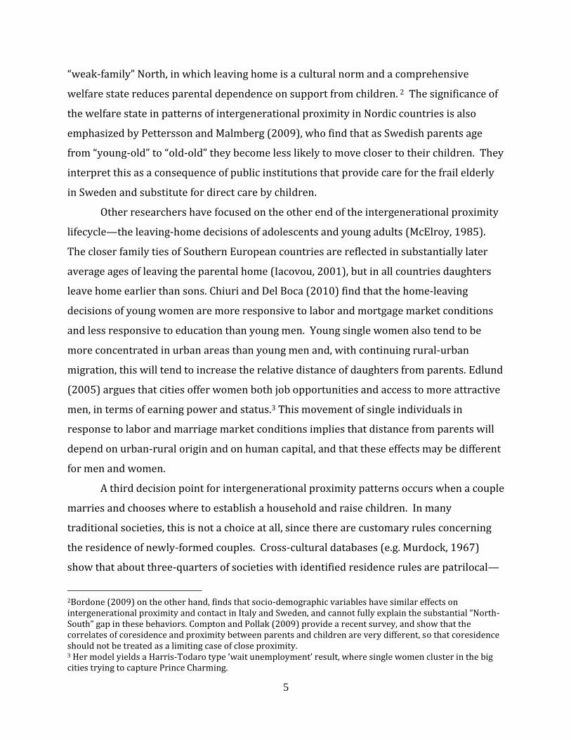
The gender difference in mobility highlighted in the Statistics Norway study is

reflected in our recent cohorts of young adults. Figure 1 shows the fraction of the total

sample of men and women from the 1967-1972 birth cohorts in discrete categories of

distance from parents at age 20 and at age 34. At age 20, most young men and women live

relatively close to home, but men are more likely to live in the same neighborhood as their

parents than are women.15 At age 34, men are more likely than women to live in the same

neighborhood as their parents and women are more likely than men to live in a different

municipality or farther away.16

Marriage and location

Table 1 presents distance from parents and other characteristics for the 1967 to

1972 birth cohorts for men and women who were legally married by age 34 and those who

were unmarried. We can link individuals only if they are legally married and, though

nonmarital cohabitation has increased in Norway,17 almost all women who will eventually

marry have married by age 34.18 Most first births in Norway are to cohabiting couples, but

15 Note that there are measurement issues concerning distance to parents around time of entering higher education as students normally register at their parents place when they study. In further analysis we will therefore focus on distance to parents during last year of education, with location measured at the educational institution. 16 All differences in Figure 1 are statistically significant (the sample consist of 417590 individuals). 17 By 2005-2007 about one in four couples were cohabiting rather than legally married. 18 Statistics Norway estimated in 2002 that by age 50 about 37 % of men and 34 % of women remain unmarried. By age 34, 51 % of men and 39 % of women in our sample are not married. In our main analysis we focus on married women by age 34 and their respective husbands (without age restriction) and so include a large majority of married couples.

11

most higher-order births occur within marriage (Perelli-Harris, Sigle Rushton, Lappegård,

Jasiloniene, DeGuilio, Keizer, Koeppen and Kostava, 2009).19 The gender difference in

distance from parents, though it is particularly pronounced for unmarried men and

women, persists in the married sample. Married women live on average farther away from

parents and are substantially less likely to live in the same neighborhood as their own

parents than married men are. They are also much more likely to live in a different

municipality, or even a different county.20

Since age at marriage is higher for men than women, married women in our sample

are slightly more likely to have children by age 34 than married men.21 Women are more

likely than men to have attended college, and this is consistent with overall gender

differences in college attendance in Norway.22 The average age at the completion of

education is around 25 years.23 Though men are less likely to attend college, their school

completion is delayed by compulsory military service. These are more educated cohorts

than their parents – only 17 to 20 percent of fathers and 9 to 10 percent of mothers of these

young adults have attended college.

Considerable rural-urban migration is still occurring in Norway and more than one-

third of young adults in these cohorts whose parents were in a rural area when the child

was age 20 are in urban locations by age 34. Though married men and women have almost

the same likelihood of migrating from rural to urban areas, there is a large gender

discrepancy in the mobility of the unmarried. While 32% of unmarried men at age 34 with

a rural origin move to an urban location, the same applies for about 40% of unmarried

women.24

19 Completed fertility in Norway is 1.9 children and has been fairly stable since the mid-1970 (Hoel, 2009). 20 Malmberg and Pettersson (2007) find that adult children in Sweden who are female, well-educated, and childless are more likely to live in a different region than their elderly parents. 21 Registry data links children to their mothers, so the number of children for married men at age 34 is constructed by linking married men to their spouses. As we cannot link unmarried men to their wives, we do not know whether they have children. 22 Statistics Norway reports that 60% of college attendees are female (Andreassen, 2008). 23 The data on age of completion of education also contains post-qualifying education which drives the average age up. The majority of these cohorts do not attend college and will end their education at age 16 (9 years of education) or 19 (12 years of education). 24 This is consistent with Edlund (2005), who shows that in most European and American countries, there is a surplus of young women in urban areas and a shortage in rural regions.

12

To investigate whether excess female distance at age 34 for the married sample is

the consequence of early moves away from parents by young women (to distant colleges,

for example, where they meet their eventual husbands), we also measured distance from

parents during the final year of education for the individuals that are married by age 34.

The location of the school is used as the cohort member’s location, since many students

who are in fact resident at colleges will be registered at their parents’ address.25 In Figure

2 we see that at school completion, there is no excess female distance from parents. In fact,

there is a tendency for females to live closer to parents at school completion than males

(more females in category 1 and more males in category 2) and there is no statistically

significant gender difference in distance categories 3 and 4.

Couples

We now focus on the joint location decisions of married couples, and in particular

those couples for whom location presents a potential conflict, i.e., couples whose parents

do not live near each other. We restrict the sample to women who are married at age 34,26

and link them to husbands with no restriction on his age. Most couples cohabit before

marriage, and we use the postcode location of each partner to establish the year in which a

particular couple probably began cohabiting.27 Table 2 shows parental distance and other

characteristics for both the full sample of couples and the analysis sample of couples whose

parents live in different municipalities.28 Studying the average distance from parents at

two points in time, during the year after beginning cohabitation and at age 34, show a very

similar pattern--wives live further away from parents than do husbands. The gender

difference in distance from parents persists within couples in both samples, and these

differences in location are all statistically significant. The analysis sample of couples with

parents who live in different municipalities and therefore have a potential location conflict

25 Distance category 0 is then unobserved since location of school is measured at the municipality level. 26 This is because we can only follow the individuals to 2006 and then our selected cohorts are 34-39 years old. As shown above, we include most of the first marriages by focusing on women married by age 34. We obtain very similar results if we construct the symmetric sample focusing on males married by age 34 and their wives. 27

Limiting the sample in this way is not very restrictive, since most couples who marry do so before she is 34, but our results may not be representative of the decisions of continuously-cohabiting couples. 28

We have also experimented with parents in different counties and get similar results.

13

(about 50 percent of all couples) is, not surprisingly, more educated and more distant from

parents than the full sample. This is a selected sample of couples who have married despite

growing up far apart, and who are therefore likely to be more mobile and perhaps less

attached to their parents than the average.

Figure 3 shows the relative distance to parents for these couples when she is aged

34. The first panel shows that more couples live closer to his parents than her parents:

approximately 45% of couples live relatively closer to his parents, 35% to her parents and

20 % live in the same distance categories to both sets of parents. Panel 2 splits the sample

by his college status, and shows that the tendency to patrilocal residence choice is confined

to the no-college subsample. For couples in which the husband has attended college, there

is no significant distance in relative distance to their respective parents.

Place or parents?

Moving close to one’s childhood home can offer two advantages: closer interaction

with parents, and access to other social ties, such as a network of old friends. For a

subsample of individuals in the 1967 to 1972 birth cohorts, we can separate these effects

because parents have moved to another county after the child is age 20 (5.4 % of the

sample). We find evidence that the principal attraction is to the parents, although

childhood home also matters. For women, 33 % live closer to their childhood home versus

46 % closer to their parents. For men the picture is roughly the same, but they are slightly

more likely to live closer to their childhood home (38 %) and less likely to live closer to

their parents (41 %).29 It is possible that the potential service exchange within women’s

extended family is more valuable, while the social or occupational networks of men’s

original childhood place are more important.

4. A Model of Couple Location

Norway is a modern, post-industrial economy, where young couples tend to

establish independent households, rather than co-residing with either set of parents.

However, distance from parents may still influence employment opportunities, household

29 The gender difference is statistically significant.

14

resource flows, and intergenerational social interactions, and these factors must be taken

into account when choosing place of residence. In this section, we formalize our discussion

of these forces by sketching a model of location choice in which relative distance to parents

is a key factor and explore the role of education, rural origin and family characteristics on

these decisions.

Initially, we abstract from joint marital decision-making, and consider individual

location choice and parental proximity. An agent chooses a location, L, that maximizes his

or her utility, and utility depends upon the consumption of a vector of private goods, X,

purchased in the market and a vector of household goods, G, produced with inputs of family

time and other resources. G will include the well-being of the children and parents of the

decision maker. Household goods are public in the sense that the decision maker’s spouse

and/or siblings also derive utility from them, but valuation may vary across members of an

extended family.

Location is defined by distance from parents, and L can take two values, 0 for

“home” and 1 for “away.” We expect that the location choice will involve a tradeoff

between employment opportunities and family ties. Location affects the agent’s income,

and therefore private goods consumption, because job opportunities vary across space, and

pursuing them will often require moving away from home. Education increases expected

distance from parents, because the labor markets for more-highly skilled jobs are

geographically larger, and this education effect on distance may be larger if the parents are

in a rural location, since high-skill jobs are concentrated in urban areas.

On the other hand, parental proximity may itself increase employment

opportunities if parents provide access to job networks or to capital, such as a farm or

family business. If this effect is stronger for men, then it may be the source of a patrilocal

residence pattern. Kramarz and Skans (2007) find that family networks have an important

influence on the transition from school to work in Sweden, and particularly for less-

educated men, who tend to follow their fathers into jobs.

Household public goods, G, including the wellbeing of children and parents, will be

enhanced by inputs of family time, affection, and other services. The cost of supplying

these inputs will be increasing in distance from family members, and will depend on family

size and other characteristics. For example, geographic proximity to your parents will

15

reduce the cost of grandparent-provided care for your children, or of providing help for

your parents as they age, but siblings may provide substitutes for both services and reduce

the value of choosing a location close to parents.

The individual’s problem is thus to choose a location L=0,1 that maximizes U(X,G)

subject to a budget constraint PX=Y(L;e,r) and a household goods production function

G=g(f) where e is education, r is rural-urban location of parents, and f=f(L;z) is a vector of

family services that will depend upon location and family characteristics, z, such as age of

parents, number of siblings, and family wealth. We let education take two possible values,

high=1 and low=0, and the parents’ location r is either urban, 0, or rural, 1. Thus the choice

to live near parents (L=0) or far from parents (L=1) will depend upon the individual’s

education, parental location, and family characteristics.

As an example, let the value of family services depend only on distance from

parents, and not on education or whether the parents live in an urban or rural location. If

an individual lives near his parents the level of family services contributed to the

household good is ff and if he lives far away it is ff with 0 . We suppose

that each person receives a nonrandom level of income if they remain at home near their

parents that depends on their education level, and that if they move away, their earnings

opportunities depend on their education level ),( 10 yy and a random component, . Since

high-education individuals are hired in a regional or national labor market, they can expect

to pay an earnings penalty, , if they restrict their employment to jobs close to home, but

that earnings penalty will be lower, αμ (α<1), if home is in an urban area with a greater

concentration of jobs. Low-education individuals are assumed to face the same average

earnings opportunities everywhere. So, individuals in four different situations (high and

low education, rural and urban parents) face the following moving decisions:

If e=0 and r=0,1, choose L=1 (“away”) if ),(),( 00 fyUfyU

If e=1 and r=1, choose L=1 if ),(),( 11 fyUfyU

If e=1 and r=0, choose L=1 if ),(),( 11 fyUfyU

In each case, the individual will move far from his or her parents if the utility of the

expected increase in income exceeds the value of the lost family services. In this simple

16

model of individual mobility, the probability of moving away will be a positive function of

education and a negative function of the family services lost to moving, and the education

effect will be larger if the parents are in a rural location, so that P(L=1; e,r,z). If the earnings

returns to moving away are larger for rural-origin workers with low education as well as

those with high education, then the probability of moving will also depend upon parent’s

location, r, directly. The marginal value of family services lost due to distance will depend

upon family characteristics such as size and wealth, and on the presence of young children

in the household. Family wealth would seem to have an ambiguous effect on location;

greater parental resources increase the attractiveness of staying home near wealthy

parents, but may also be able to reduce the costs of distance through travel and improved

communication.

For a two-person household consisting of a man, m, and a woman, w, whose parents

live in different locations, we can think of a joint location decision L(m,w) that consists of

choosing among three locations: his home, L(0,1); her home, L(1,0), or away, L(1,1). The

simplest way to model a couple’s joint location decision is a unitary family framework in

which the couple jointly maximizes a welfare function W(X,G) subject to pooled constraints

wm yyPX and )( wm ffgG . The vector of household goods, G, now includes the

utility of both sets of parents, and partners may have different levels of concern for their

own parents’ wellbeing and that of their in-laws. In this model, the husband’s and wife’s

family characteristics will affect inputs to the household good and the employment

opportunities of both partners affect earnings and market goods consumption. 30

The couple’s distance to both sets of parents will be jointly determined, with the

education of both partners pulling the couple outward and towards the principal urban

centers, while each parental location exerts a gravitational pull whose force depends on the

value of family exchanges and of local employment opportunities. The probability of living

farther from her parents than his is simply π(W(0,1)>W(1,0)) which will be increasing in

her education and decreasing in his, increasing in his family services and decreasing in

30

For simplicity we assume that the couple takes for granted the location of both sets of siblings, so strategic

interaction among siblings is neglected. The formulation of the welfare function is general enough to possibly

include that an individual may care for the utility a sibling gets from higher utility for common parents, but this is

not given central attention.

17

hers, increasing in his parent’s urban location and decreasing in hers. If the relationship

between education and earnings is identical for men and women, then the education effects

on relative location will also be symmetric. However, since men tend to work more hours

than women, men’s education may have a greater weight in household income, and

therefore on location decisions. Similarly, if matrilineal ties across generations are closer,

then the presence of children (and own-family characteristics) may exert a stronger pull

towards the wife’s family of origin.

Alternatively, we can treat joint location as a bargaining problem in which the

husband and wife have different preferences concerning elements of the household public

goods vector, i.e. she places more value on goods that are enhanced by proximity to her

parents, and he prefers proximity to his parents. We can treat the couple as though they

are maximizing a weighted average of their individual utilities, in which the weight on the

husband’s utility, , is a function of his, and his family’s, contributions to the household’s

resources.

),()),;,(1(),(),;,( GXUfyfyGXUfyfyV wwwmmmwwmm

In this case, factors that affect the relative bargaining power of each partner in the joint

decision process, such as own earnings potential or parental wealth, will also affect relative

distance from parents. In this non-unitary framework, a patrilocal residential pattern may

result from the greater bargaining power of husbands combined with a preference for

locating close to one’s own family, and could represent a form of geographic oppression of

women.

If we assume that each partner prefers to locate closer to his or her own family, then

the bargaining framework allows for some results that would be inconsistent with the

unitary model. Given the evidence that mother-daughter ties in the provision of care

services are stronger, for example, if we find that family characteristics have a stronger

impact on proximity to his parents rather than hers it may reflect the influence of his

preferences on a bargained outcome power, rather than a joint maximization of family

services. Similarly, if education brings individuals closer to his-her family of origin, rather

than pushing them further away in pursuit of employment options, this may indicate that

18

potential earnings are strengthening an individual’s influence, relative to his spouse’s, on

joint location.

Some particular characteristics of the Norwegian labor market and the provision of

public services may affect the location decisions of couples as represented in this model.

The labor market participation of women in Norway is very high31, and women are able to

maintain consistent job attachment because of generous parental leave32 and the increased

availability, over the last few decades, of high quality child care at subsidized prices. There

has also been a substantial expansion in public nursing homes for the elderly (though

access is rationed) and this is likely to have reduced family responsibilities for eldercare,

which are disproportionately borne by women. Thus, the employment opportunities of

women may be relatively important in determining couple location in Norway, and

publicly-provided care for children and the elderly may have weakened the links between

women and their mothers.

5. Results

The administrative registry data described in Section 3 can be used to explore the

determinants of intergenerational residence patterns, including the relative distance from

parents of young married couples. The effects of employment opportunities and family

characteristics on distance from parents is examined here with two different empirical

models: an ordered logit model of individual distance from parents for all married men

and women in the birth cohorts 1967-1972, and a multinomial logit model of relative

distance from parents for married couples whose parents live far apart.

We see the two empirical strategies as complements. The first investigates the

determinants of distance to parents for individuals, with a focus on differences between

men and women with the same characteristics. The second strategy investigates relative

distance to parents for couples for whom location presents a potential conflict, since his

parents and her parents live far apart. By excluding couples whose parents live in the same

municipality we are left with a selected subsample of (possibly more mobile) young men

31 In 2005, 70% of all women aged 16-74 and 82% of women aged 25-54 were employed (Statistics Norway, 2005). 32 Parents are entitled to 46 weeks with full coverage or 54 weeks with 80 % coverage.

19

and women. However, we can observe the decisions, conditional on parental location, of

couples who need to balance competing demands for parental proximity.

Individual distance to parents

Table 3 reports the estimated coefficients from an ordered logit model of distance

category from parents for the pooled population of married males and females from 1967-

1972 birth cohorts. We report odds ratios that can be interpreted as follows: for a unit

increase in explanatory variable kx , the odds of a lower outcome compared with a higher

outcome are changed by the factor )exp( k , holding all other variables constant.

The first column shows that the gender effect on distance persists in a model with

individual and family controls—the odds of living in farther distance categories from

parents at age 34 is 16% larger for females than males.33 Also as expected, attending

college drives you away from parents and this effect is even larger for the college-educated

whose parents live in rural areas. For the non-college group, however, rural parents are

associated with greater proximity.

Family characteristics also matter. We find that having no or one sibling (compared

to two or more siblings) moves you closer to your parents, while there are few significant

effects of birth order.34 The odds of living in a farther distance category from parents are

60% larger for couples with no children. This is consistent with the expectation that

children increase the value of family connections, and pull you towards your parents.

Having a college-educated mother or father also increases distance. This may be because

parental wealth reduces the effective cost of maintaining family ties over longer distances

or, alternative, parental education may be correlated with the completed education or

professional qualifications of children, and so with the returns to a central location.

Columns 2 and 3 show the distance model estimated separately by gender. The most

interesting differences are in the effects of college attendance and rural-urban origin.

Attending college increases parental distance more for men than for women, and the

33

When we use earlier measures of distance to parents like year after cohabitation the gender effect is even larger.

Also note that if we run the ordered logit without any individual or family controls we obtain almost the identical

gender coefficient. 34

This is consistent with the findings of Rainer and Siedler (2009) and Compton and Pollak (2009). This result

is not directly comparable to Konrad, et al. (2002) who find that older siblings tend to move farther away from

parents, since they do not control for family size.

20

interaction effect of college and rural parents is also much larger for men. For the non-

college educated, rural parents increase distance for women and reduce distance for men.

The relative immobility of non-college educated, rural men is striking.

Table 4 reports the size of the gender effect alone for four separate ordered logits

with the sample split by college attendance and rural-urban origin. This shows that the

patrilocal residence pattern of young couples is driven solely by the non-college group and

especially by the non-college group with rural parents. The odds of living in farther

distance categories from parents at age 34 is 62% larger for females than males in the non-

college and rural parents group and 32% larger for the non-college and urban parents

group. In the college-educated samples, irrespective of rural-urban origin, there is a

modest tendency towards matrilocality.

Given these results, it seems important to model the behavior of the college and

non-college groups separately, and examine how the determinants of parental distance

vary between men and women. In Table 5, the ordered logit model is estimated separately

for four groups—college-educated men, college-educated women, non-college men, and

non-college women. For three of these groups, the effects of family characteristics on

distance are very similar, while the determinants of distance for the male, non-college

group are very different—in some cases even different in sign. Rural parents drive all

women and college-educated men away from parents, but are associated with greater

proximity for non-college educated men. Also, more siblings increase distance from parents

for the three groups, while siblings bring non-college men closer to their family of origin.

Birth order has few significant effects. The fact that men’s family ties exert a stronger

gravitational effect among the less-educated than do women’s indicates that either family

ties have a different impact on couple wellbeing for this group, or that men’s preferences

for family proximity have more influence on the couple’s location decisions.

These results help us to establish a convincing and robust first finding. On average,

married men in Norway live much closer to their parents than do married women, and this

difference is present at all stages in a couple’s early location decisions through age 34.35

This difference is not explained by other observed characteristics, but allowing for

35 Estimates at different lifecycle points, after the couple starts cohabiting, yield similar results. The gender differences are largest during the year after cohabitation.

21

heterogeneous gender effects shows that this apparent patrilocality is limited to the

subpopulation who have not attended college.

Relative Distance to Parents for Couples

We turn now to a within-couple estimation where we examine the effects of both

partners’ characteristics on their relative distances to his and her parents. We restrict

attention to couples who have a potential geographical conflict, so that couples where both

sets of parents live at the same place are excluded. This means that our estimates are

conditional on parent’s location, and thus on the matching of husbands and wives. Our

basic specification is a multinomial logit model in which the base outcome is that couples

live equally distant (i.e. in the same distance category) from his parents and her parents,

and the alternatives are that the couple lives farther from her parents than from his

parents or that they live farther from his parents than from hers. More specifically we have

the following multinomial logit model;

bmbm xxby

xmyx ||

)|Pr(

)|Pr(ln)(ln

for 2,1m (1)

where b is the base outcome and m=1,2 are the alternative outcomes. We compute marginal

effects of each covariate evaluated at the mean of all the other variables. A Hausman test of

independence of irrelevant alternatives comparing the three-outcome full model with

restricted models fails to reject independence.

Marginal effects from the multinominal logit model, evaluated at the means of the

independent variables, are reported in Table 6.36 Education, rural origin, family size and

the presence of children all have substantial and significant effects on relative location, and

the results are for the most part consistent with those of the individual distance models.

College attendance by either the husband or the wife is associated with the couple being

less likely to live closer to own parents, relative to the same distance or closer to spouse’s

parents, but the effects of husband’s education are several times larger than the effects of

wife’s education. An urban-origin woman who has attended college is 1.9 % less likely to

36 We obtain very similar results when estimating the same models with distance measured at year after cohabitation and year after having first child as the dependent variables.

22

live close to her parents than one who has not, but an urban-origin man who has attended

college is 8.1 % less likely to live closer to his parents. The interaction effects between

college and rural parents reinforce this contrast—college has a stronger distancing effect

from rural parents and the size of this effect is much stronger for husbands. For the non-

college sample, rural parents have a distancing effect, but if both spouses are of rural origin

the couple will tend to live closer to his parents.

Family ties have effects on relative distance that are consistent with the individual

distance results. Couples with children are more likely to live either closer to his parents or

closer to hers, relative to living the same distance away. His and her number of siblings

also exhibit roughly symmetric effects on relative distance: If she has fewer siblings they

live closer to her parents and if he has fewer siblings they live closer to his parents.

We know from previous results that the gender difference in distance to parents is

particularly pronounced in the non-college group, and that the determinants of individual

distance from parents are distinctly different for less-educated men. We therefore estimate

the relative distance model separately for samples in which the husband has attended

college (Table 7a) or not (Table 7b).37 In the individual distance model we found that

family ties, measured by number of siblings, had a different effect on location for non-

college educated men than for women or college-educated men. For this group, more

siblings reduced, rather than increased, distance from parents, and we speculated that

family and social networks may be of higher value to non-college men. In the relative

distance model, we find that a couple tends to locate closer to the parents of the partner

with few siblings, though the effect of siblings for non-college educated men, is much

smaller (half the size) than for the college educated. A possible explanation is that men

who place a higher value on family and local social ties are also more likely to marry a

hometown girl, and thus be excluded from the relative distance sample.

Both the individual distance model and the relative couple distance model confirm

the basic patrilocality result. Married couples move closer to his parents, and this is

basically driven by the non-college group. Having more siblings is a much stronger push

37 The results are evaluated at the mean of the independent variables for the two groups separately, however, they are roughly comparable as we have tested the effects for the two groups giving them the characteristics of the other group and this does not significantly change the coefficients.

23

factor away from his parents for couples where he has attended college than for couples

where he has not attended college. Since patrilocality seems to be so closely associated

with the families of the non-college educated men, especially those with rural parents, it is

possible that father-son economic ties are stronger for this group. We turn to this question

in section 6.

Robustness test

We have estimated a number of alternative specifications of our model to check its

robustness.38 Different sets of controls do not affect any of the main results on patrilocality

and the importance of family ties. The exclusion of some counties in Norway that are likely

to have different individual migration and couple location patterns (such as Oslo, which is

both the capital and is both a municipality and a county, and the three northern counties

that have experienced substantial outmigration), also does not affect our results.

6. Discussion and Further Analysis

One possible explanation for the excess female distance from parents among

married couples could be that the husband’s labor market prospects dominate the location

decision of married couples, and that local social networks and family ties are particularly

important for the job opportunities of less-educated men.39 The gender asymmetry in this

story requires either that more weight be placed on male employment prospects than

those of the wife, or in a greater importance of family ties in men’s job placement. In the

latter case, this effect may be more pronounced for men who work in male-dominated

occupations, where they are likely to follow their fathers into work in a particular industry

or even for a particular employer. Alternatively, a son may join and later inherit his

father’s business—farming is one example in which this is common.

The Living and Moving Survey asks if the respondent’s family owns ´productive

capital, referring to farms, fishing vessels and various small businesses. Of all respondents,

14% answer yes to this question, slightly higher for men than for women. The importance

38 These results are available upon request 39 This would be consistent with the Swedish school-to-work transition results of Kramarz and Skans (2007) and also the findings by Sørlie (2008).

24

of productive capital is higher in more peripheral areas, where 27% report that they own

such capital.40 Formally, men and women have the same inheritance rights to this type of

capital, but if men are more likely to take over and utilize these assets, this may explain

why rural, less educated men seem to be more tied to their place of origin than other

groups.

For about 30% of our observations, an individual’s occupation can be matched with

parental occupations.41 We can test the family employment ties hypothesis by comparing

the gender differences in location when the son is (or is not) in the same occupation as his

father and when the daughter is (or is not) in the same occupation as her mother. We

separate the sample into male-dominated occupations (managers,

agriculture/fishery/forestry, industry and crafts) and female-dominated occupations

(health, services and office workers) and compare relative distance to parents for three

groups—same-sex parent and child are in the same occupation, not in the same occupation,

or occupation is missing.42 The first panel in Figure 4 shows that, for all three father-son

groups, couples are more likely to live closer to his parents but the difference is much

larger for couples for whom father and son are in the same occupation. For this subsample,

nearly 50% of couples live relatively closer to his parents while 30% live relatively closer

to her parents. For the two other groups these proportions are approximately 40% and

35%. In panel 2 we see that, in the three groups based on mother-daughter occupational

ties, more couples live closer to his parents, but there are no significant differences across

subsamples.

Table 8 shows the results of the multinomial logit model for relative distances.

Model 1 shows that a father and son in same male-dominated occupation is positively

associated with couple location that is closer to his parents and farther from hers.

Interacting the father-son dummy with rural origin and college status (Model 2), we find

that this is mainly driven by father-son occupational ties when the parents are rural, so that

40 Among people living in the periphery and who never moved, the figure increases to 37%, 41 Unfortunately we do not have data on occupations for everyone, especially parents. We have tested if this is a highly selected sample and find that the gender results and the characteristics of distances are very similar to the total sample results. 42 This classification is based on registry data for the total sample of 1967-1972 cohorts and group occupations according to whether the occupation has more than 75 % of either males or females.

25

agriculture and resource-based industries account for much of this effect. Mother-daughter

occupational ties have no significant effect on individual or couple location patterns.

We need to interpret these last findings with care, since location choices could be

driving occupational continuities between father and son, rather than the reverse. For

example, if men’s preferences for proximity to family and friends dominate those of

women, this may explain why rural and non-college men find jobs close to their place of

origin, and these are likely to be in their fathers’ occupations. Pettersson and Malmberg

(2009) find that “moving home” to a rural area (and close to an elderly father) is a common

feature of migration patterns in Sweden, and suggest that this may be a remnant of a

patrilocal tradition. The father-son occupational ties that we observe in the Norwegian data

suggest that family and employment networks interact in shaping preferences for place of

residence. Bye (2009) suggests that young rural Norwegian men build masculine identities

in which hunting, outdoor life and handyman skills are important and that this identity in

turn fosters loyalty to place. Such identity formation interacts with ownership of farms and

other types of rural productive capital, yielding a location pattern in which rural, less

educated men are strongly tied to their place of origin, relative to women and to college-

educated men.

In conclusion, we find that in Norway there is a strong pattern of patrilocality in the

location decisions of young married couples, who are more likely to live closer to his

parents than to her parents. This pattern is very pronounced for husbands who have not

attended college and whose parents live in a rural location. We also find some evidence

that family ties, in the form of siblings, play a very different role for non-college males than

the other groups. Siblings are associated with more distance from parents for the college-

educated and for all women, but not for non-college married men. Family ties may interact

with the local employment networks, and we find that men in the same male-dominated

occupations as their fathers tend to live near his parents, though no such pattern is evident

for women’s occupations. Despite evidence that intergenerational resource flows, such as

childcare and eldercare, are particularly important between women and their parents, the

family connections of husbands appear to dominate the location decisions of less-educated

married couples.

26

References

ANDREASSEN, K. (2008): "Cohabitation 2008." Statistics Norway,

http://www.ssb.no/english/subjects/02/01/20/samboer_en/.

BAKER, M. J., and J. P. JACOBSEN (2007): "A Human Capital-Based Theory of Postmarital

Residence Rules." Journal of Law, Economics, and Organization, 23, 208-241.

BORDONE, V. (2009): "Contact and Proximity of Older People to Their Adult Children: A

Comparison between Italy and Sweden." Population, Space and Place, 15, 359-380.

BYE, L. M. (2009): "How to Be a Rural Man: Young Men's Performances and Negotiations of

Rural Masculinities." Journal of Rural Studies, 3, 278-288.

CHIURI, M. C., and D. DEL BOCA (2010): "Home-Leaving Decisions of Daughters and Sons."

Review of Economics of the Household, 8, 398-408.

COMPTON, J., and R. A. POLLAK (2007): "Why Are Power Couples Increasingly Concentrated in

Large Metropolitan Areas?" Journal of Labor Economics, 25, 475-512.

COMPTON, J., and R. A. POLLAK (2009): "Proximity and Coresidence of Adult Children and

Their Parents: Description and Correlates." Working paper, University of Michigan.

COSTA, D. L., and M. E. KAHN (2000): "Power Couples: Changes in the Locational Choice of the

College Educated, 1940-1990." Quarterly Journal of Economics, 115, 1287-1315.

COX, D. (2003): Private Transfers within the Family: Mothers, Fathers, Sons and Daughters. In

Death and Dollars: The Role of Gifts and Bequests in America, A. Munnell and A.

Sunden, eds. Washington, DC: Brookings Institution Press.

EDLUND, L. (2005): "Sex and the City." Scandinavian Journal of Economics, 107, 25-44.

EGERBLADH, I., A. B. KASAKOFF, and J. W. ADAMS (2007): "Gender Differences in the Dispersal

of Children in Northern Sweden and the Northern USA in 1850." The History of the

Family, 12, 2-18.

GREENWELL, L., and V. L. BENGTSON (1997): "Geographic Distance and Contact between

Middle-Aged Children and Their Parents: The Effects of Social Class over 20 Years."

The Journals of Gerontology: Series B, 52, 13.

HANK, K. (2007): "Proximity and Contacts between Older Parents and Their Children: A

European Comparison." Journal of Marriage and Family, 69, 157-173.

HOEL, E. (2009): "Population Statistics. Births. 2009." Statistics Norway,

http://www.ssb.no/english/subjects/02/02/10/fodte_en/.

IACOVOU, M. (2001): "Leaving Home in the European Union." ISER Working Paper 2001-18.

JACOBY, H. G., and G. MANSURI (2010): "Watta Satta: Bride Exchange and Women's Welfare in

Rural Pakistan." American Economic Review, 100, 1804-1825.

KONRAD, K. A., H. KUNEMUND, K. E. LOMMERUD, and J. R. ROBLEDO (2002): "Geography of

the Family." American Economic Review, 92, 981-998.

KRAMARZ, F., and O. N. SKANS (2007): "With a Little Help from My... Parents? Family

Networks and Youth Labor Market Entry." CREST Working Paper.

LAWTON, L., M. SILVERSTEIN, and V. BENGTSON (1994): "Affection, Social Contact, and

Geographic Distance between Adult Children and Their Parents." Journal of Marriage

and the Family, 56, 57-68.

LEONETTI, D. L., D. C. NATH, and N. S. HEMAM (2007): "The Behavioral Ecology of Family

Planning in Two Ethnic Groups in N.E. India." Human Nature, 18, 225-241.

27

MALMBERG, G., and A. PETTERSSON (2007): "Distance to Old Parents." Demographic Research,

17, 679-704.

MCELROY, M. B. (1985): "The Joint Determination of Household Membership and Market

Work: The Case of Young Men." Journal of Labor Economics, 3, 293-316.

MINCER, J. (1978): "Family Migration Decisions." Journal of Political Economy, 86, 749-773.

MURDOCK, G. P. (1967): Ethnographic Atlas. University of Pittsburgh Press.

MØEN, J., K. SALVANES, and E. SØRENSEN (2004): "Documentation of the Linked Employer-

Employee Data Base at the Norwegian School of Economics and Business

Administration." mimeo, Norwegian School of Economics.

PERELLI-HARRIS, B., W. SIGLE RUSHTON, T. LAPPEGÅRD, A. JASILONIENE, P. DEGUILIO, R.

KEIZER, K. KOEPPEN, and D. KOSTAVA (2009): "Does Childbearing Change the Meaning

of Cohabitation? Examining Nonmarital Childbearing across Europe." Paper presented at

the 2009 Population Association of America meeting.

PETTERSSON, A., and G. MALMBERG (2009): "Adult Children and Elderly Parents as Mobility

Attractions in Sweden." Population, Space and Place, 15, 343-357.

RAINER, H., and T. SIEDLER (2009): "O Brother, Where Art Thou? The Effects of Having a

Sibling on Geographic Mobility and Labour Market Outcomes." Economica, 76, 528-

556.

— (2010): "Family Location and Caregiving Patterns from an International Perspective." CESifo

Working Paper No. 2989.

ROSENZWEIG, M. R., and O. STARK (1989): "Consumption Smoothing, Migration, and Marriage:

Evidence from Rural India." The Journal of Political Economy, 97, 905-926.

SWEETSER, D. A. (1963): "Asymmetry in Intergenerational Family Relationships." Social Forces,

41, 346-352.

SØRLIE, K. (2008): "Bo- og Flyttemotivundersøkelsen 2008." Statistics Norway/ Norwegian

Institute for Urban and Regional Research. Presented at Demografisk Forum (only in

Norwegian).

28

Figure 1: Distance from parents at age 20 and age 34 Total 1967-1972 Norwegian birth cohorts

29

Figure 2: Distance from parents during the final year of education 1967-1972 Norwegian birth cohorts married by age 34

30

Figure 3: Relative Distance to Parents when Wife is Aged 34 1967-1972 cohorts of married women and their husbands

Analysis sample with parents in different municipalities

31

Figure 4: Relative Distance to Parents when Wife is Aged 34 1967-1972 cohorts of married women and their husbands

Analysis sample with parents in different municipalities Matched parent-child occupations

32

Table 1: Distance from Parents and Descriptives for the 1967-1972 Cohorts by Marital Status at Age 34

Married

men Unmarried

men Married women

Unmarried women

Distance from parents at age 34

Average distance: 1.53 1.38 1.62 1.63

Distance from parents at age 34 (%):

0: Same neighborhood .297 .370 .253 .271 1: Same municipality, different neighborhood

.265 .248 .274 .265

2: Same county, different municipality

.178 .138 .210 .173

3: Same region, different county .126 .121 .131 .143

4: Different region .134 .124 .133 .147

Individual and family characteristics:

Age at marriage 28.11 - 26.41 -

Have children by age 34 .78 - .85 .52

Education

Attended college .35 .28 .43 .41

Age at completion of education 25.13 24.79 25.49 25.96

Mother attended college .10 .09 .10 .09

Father attended college .20 .17 .19 .17

Family size

No siblings .05 .06 .05 .06

1 sibling .34 .36 .34 .37

2 siblings or more .61 .58 .61 .57

Birth order

1st born .40 .40 .40 .39

2nd born .32 .31 .31 .32

3rd born or later .29 .29 .29 .29

Urban residence at age 34: If rural origin (parents rural when child was age 20)

.368 .321 .386 .403

If urban origin .963 .963 .951 .953

N 88068 107803 108818 79682

33

Table 2: Distance from Parents and Descriptives for Married Couples - 1967-1972 cohorts of women and their husbands

Total sample and analysis sample with parents in different municipalities

Total sample Parents do not live in the same

municipality

A Wife

B Husband

Diff. (A-B)

C Wife

D Husband

Diff. (C-D)

Average distance from parents in young adulthood (0-4): Year after beginning cohabitation

1.60 1.41 .188*** (.006)

2.05 1.81 .248*** (.008)

When she is aged 34 1.62 1.47 .143*** (.006)

2.16 1.98 .176*** (.006)

Distance from parents when wife is aged 34 (%):

0: Same neighborhood .253 .319 -.066*** (.002)

.149 .218 -.069*** (.002)

1: Same municipality .274 .259 .015*** (.002)

.131 .140 .009*** (.002)

2: Same county .210 .178 .032*** (.002)

.323 .270 .058*** (.003)

3: Same region .131 .119 .012*** (.002)

.193 .180 .013*** (.002)

4: Different region .133 .126 .007*** (.002)

.199 .191 .008*** (.002)

Individual and family characteristics:

Age at marriage 26.43 29.33 -2.87*** (.019)

26.76 29.12 -2.36*** (.025)

Attended college .428 .330 .098*** (.002)

.482 .389 .093*** (.003)

Mother attended college .097 .088 .008*** (.001)

.111 .107 .003* (.002)

Father attended college .187 .177 .010*** (.002)

.208 .206 .002

(.002)

No siblings .049 .047 .002** (.001)

.046 .042 .003*** (.001)

1 sibling .343 .310 .034*** (.002)

.350 .320 .030*** (.003)

2 siblings or more .607 .643 -.036*** (.002)

.604 .638 -.033*** (.003)

1st born .401 .377 .024*** (.002)

.409 .403 .005* (.003)

2nd born .311 .320 -.009*** (.002)

.314 .325 -.010*** (.003)

3rd born or later .289 .304 -.015*** (.002)

.277 .272 -.005* (.003)

Note: ***significant at 1 %, **significant at 5 %, *significant at 10 %

34

Table 3: Ordered Logit Model of Distance from Parents at Age 34 (odds ratios) Married men and women from the 1967-1972 cohorts

Full Sample

Married Women

Married Men

Female 1.164***

(.010) -

-

College 1.651***

(.017) 1.412***

(.020) 2.031***

(.033)

Rural origin .900*** (.012)

1.031* (.019)

.769*** (.015)

Rural * College 1.734***

(.037) 1.452***

(.040) 2.220***

(.074)

No siblings (relative to two or more) .900*** (.021)

.842*** (.025)

.976 (.034)

One sibling (relative to two or more) .976** (.010)

.944*** (.013)

1.01 (.016)

1st born (relative to 3rd or more) .985

(.012) .959** (.016)

1.024 (.019)

2nd born (relative to 3rd or more) 1.003 (.012)

.989 (.016)

1.024 (.019)

No children 1.589***

(.019) 1.664***

(.028) 1.523***

(.025)

Mother’s education (college) 1.283***

(.020) 1.310***

(.028) 1.240***

(.029)

Father’s education (college) 1.369***

(.017) 1.325***

(.022) 1.398***

(.026)

Age at marriage 1.018***

(.001) 1.030***

(.002) 1.003 (.002)

Birth cohort 1968 (relative to 1967) .987

(.014) .980

(.019) .997

(.0022)

Birth cohort 1968 (relative to 1967) .965** (.014)

.934*** (.018)

1.007 (.022)

Birth cohort 1968 (relative to 1967) .942*** (.014)

.905*** (.018)

.990 (.022)

Birth cohort 1968 (relative to 1967) .928** (.014)

.892** (.018)

.978 (.022)

Birth cohort 1968 (relative to 1967) .908** (.014)

.847** (.017)

.989 (.023)

N 176442 98048 78394

Note: ***significant at 1 %, **significant at 5 %, *significant at 10 %

35

Table 4: Ordered Logit Model of Distance from Parents at Age 34 Odds Ratio on Female Dummy

Subsamples of married men and women from the 1967-1972 cohorts By education and urban/rural origin

Female dummy N

College/urban origin .911*** (.015)

54105

College/rural origin .857*** (.025)

16565

Non-college/urban origin 1.315***

(.017) 80318

Non-college/rural origin 1.620***

(.039) 25454

Note: Dummies for number of siblings, birth order, children, mother’s education, father’s education, birth cohort and age at marriage are included in all specification. ***significant at 1 %, **significant at 5 %, *significant at 10 %

36

Table 5: Ordered Logit Model of Distance from Parents at Age 34 (odds ratios) Married men and women from the 1967-1972 cohorts, by education

Married Women Married Men

College Non- college College Non- college

Rural origin 1.444***

(.030) 1.044** (.020)

1.615*** (.043)

.781*** (.016)

No siblings (relative to two or more)

.812*** (.036)

.871*** (.036)

.832*** (.046)

1.082** (.040)

One sibling (relative to two or more)

.923*** (.019)

.963* (.018)

.939** (.024)

1.060*** (.021)

1st born (relative to 3rd or more) .922*** (.012)

.992 (.022)

1.002 (.031)

1.028 (.024)

2nd born (relative to 3rd or more)

.982 (.025)

.991 (.021)

.997 (.032)

1.029 (.023)

No children 1.651***

(.038) 1.603***

(.041) 1.581***

(.040) 1.459***

(.032)

Mother’s education (college) 1.251***

(.031) 1.440***

(.062) 1.227***

(.035) 1.275***

(.052)

Father’s education (college) 1.245***

(.028) 1.239***

(.034) 1.301***

(.031) 1.522***

(.042) N 42,476 55,572 28,194 50,200

Note: ***significant at 1 %, **significant at 5 %, *significant at 10 %. Cohort dummies and age at marriage are included in all specifications.

37

Table 6: Multinomial Logit Model of Couple’s Relative Distance from Parents Married women from the 1967-1972 cohorts at age 34 and their husbands

(marginal effects)

Same distance (base outcome)

Closer to her parents

Closer to his parents

College: Wife .016*** (.005)

-.019*** (.006)

.003 (.006)

Husband .042*** (.005)

.039*** (.006)

-.081*** (.006)

Rural origin: Wife -.006 (.007)

-.121*** (.007)

.127*** (.008)

Husband -.016** (.006)

.084*** (.008)

-.068*** (.007)

Rural origin * College: Wife .037*** (.010)

-.029*** (.011)

-.008 (.011)

Husband .065*** (.010)

.032*** (.011)

-.097*** (.011)

No siblings (relative to two or more)

Wife .005

(.010) .069*** (.012)

-.073*** (.012)

Husband -.014 (.010)

-.070*** (.012)

.084*** (.013)

One sibling(relative to two or more)

Wife -.004 (.005)

.027*** (.006)

-.023*** (.006)

Husband .005

(.005) -.033*** (.006)

.027*** (.006)

1st born (relative to 3rd or more)

Wife .002

(.006) .014** (.007)

-.015** (.007)

Husband -.001 (.005)

.003 (.006)

-.003 (.007)

2nd born (relative to 3rd or more)

Wife .003

(.006) .002

(.007) -.005 (.007)

Husband -.005 (.005)

.011* (.006)

-.006 (.007)

No children .046*** (.006)

-.018*** (.007)

-.029*** (.007)

Mother’s education: Wife .018*** (.007)

.005 (.008)

-.023*** (.008)

Husband .014*** (.007)

-.019** (.008)

.006 (.009)

Father’s education: Wife .008

(.005) .000

(.006) -.009 (.007)

Husband .016*** (.005)

.011* (.006)

-.027*** (.007)

N Couples: 46100

Note: Controls for wife’s and husband’s birth cohort and age at marriage are included in all specifications. ***significant at 1 %, **significant at 5 %, *significant at 10 %

38

Table 7a: Multinomial Logit Model of Couple’s Relative Distance from Parents Married women from the 1967-1972 cohorts at age 34 and their husbands

Husband has attended college (marginal effects)

Husband: College

Same distance (base outcome)

Closer to her parents

Closer to his parents

College: Wife .043*** (.009)

-.036*** (.010)

-.008 (.010)

Rural origin: Wife .030* (.017)

-.165*** (.016)

.135*** (.018)

Husband .036*** (.008)

.115*** (.009)

-.151*** (.008)

Rural origin * College: Wife .010

(.019) .001

(.020) -.012 (.019)

No siblings (relative to two or more)

Wife -.013 (.016)

.088*** (.019)

-.075*** (.018)

Husband -.032* (.017)

-.085*** (.017)

.116*** (.020)

One sibling(relative to two or more)

Wife -.015* (.008)

.042*** (.009)

-.027*** (.009)

Husband .004

(.008) -.030*** (.009)

.026*** (.009)

1st born (relative to 3rd or more)

Wife .014

(.009) .001

(.011) -.016 (.010)

Husband -.007 (.009)

.005 (.010)

.002 (.010)

2nd born (relative to 3rd or more)

Wife .001

(.010) -.010 (.010)

.009 (.010)

Husband -.005 (.009)

.004 (.011)

.001 (.010)

No children .055*** (.009)

-.021** (.010)

-.033*** (.009)

Mother’s education: Wife .009

(.009) .012

(.010) -.021** (.010)

Husband .016* (.009)

-.022** (.010)

.005 (.010)

Father’s education: Wife .013

(.008) -.004 (.009)

-.008 (.009)

Husband .012

(.008) .002

(.008) -.014* (.008)

N Couples: 18826

Note: Controls for wife’s and husband’s birth cohort and age at marriage included in all specifications. ***significant at 1 %, **significant at 5 %, *significant at 10 %

39

Table 7b: Multinomial Logit Model of Couple’s Relative Distance from Parents Married women from the 1967-1972 cohorts at age 34 and their husbands

Husband has not attended college (marginal effects)

Husband: Non-college

Same distance (base outcome)

Closer to her parents

Closer to his parents

College: Wife .002

(.006) -.017** (.007)

.015* (.008)

Rural origin: Wife -.016 (.007)

-.108*** (.008)

.129*** (.009)

Husband -.008 (.006)

.075*** (.008)

-.067*** (.008)

Rural origin * College: Wife .039*** (.013)

-.015 (.014)

-.025* (.015)

No siblings (relative to two or more)

Wife .018

(.013) .055*** (.016)

-.072*** (.016)

Husband -.002 (.013)

-.058*** (.015)

.060*** (.017)

One sibling(relative to two or more)

Wife .004

(.006) .016** (.007)

-.020*** (.008)

Husband .007

(.006) -.035*** (.007)

.028*** (.008)

1st born (relative to 3rd or more)

Wife -.007 (.007)

.022*** (.008)

-.014* (.009)

Husband .003

(.007) .001

(.008) -.004 (.009)

2nd born (relative to 3rd or more)

Wife .005

(.007) .009

(.008) -.014 (.009)

Husband -.006 (.006)

.016* (.008)

-.010 (.008)

No children .040*** (.008)

-.015* (.009)

-.024** (.010)

Mother’s education: Wife .032*** (.011)

-.009 (.013)

-.023* (.014)

Husband .011

(.012) -.010 (.014)

-.002 (.015)

Father’s education: Wife .003

(.007) .004

(.009) -.007 (.010)

Husband .022*** (.008)

.023** (.010)

-.045*** (.011)

N Couples: 27274

Note: Controls for wife’s and husband’s birth cohort and age at marriage included in all specifications. ***significant at 1 %, **significant at 5 %, *significant at 10 %

40

Table 8: Effect of Father-Son Occupational Match on Relative Distance from Parents. Married women from the 1967-1972 cohorts at age 34 and their husbands, with father-son

occupations non-missing Multinomial logit (marginal effects)

Same distance (base outcome)

Closer to her parents

Closer to his parents

Model 1 Father-son in same occupation (Same)

-.012 (.011)

-.051*** (.013)

.063*** (.013)

Model 2

Same -.007 (.015)

-.033** (.017)

.040** (.018)

Same * Rural origin .015

(.029) -.107*** (.028)

.093*** (.035)

Same * College -.024 (.022)

.010 (.028)

.014 (.029)

N Couples: 7972

Note: Dummies for both her and his number of siblings, birth order, children, mother’s education, father’s education, birth cohort and age at marriage are included in all specifications. ***significant at 1 %, **significant at 5 %, *significant at 10 %

41

Appendix A DATASET 1 The datasets we use are created by linking different Norwegian administrative datasets. We start out by linking children born from 1967-1972 with their parents. This gives us the first dataset (used in figure 2, table 1, 3, 4 and 5) with the total population of married females and males from cohorts 1967-1972. We then have 417590 individuals where we have

information on all children and at least one of the parents. Then we add to each individual

gender, citizenship, years and type of education from the 2006 population files. Then we link individuals to spouse, number of children, marital status, postcode and

municipality of residence each year from the 1986-2006 population files

We do the same process linking mothers and fathers to respective years and type of education,

ages and postcodes and municipality of residence from 1986 to 2006.

We also add information on which year the individual completed education and in which

municipality this education was completed.

We create the following variables:

1. a dummy for being married by age 34 if you have status of being married at least one of the

years between age 20 and 34.

2. age at first marriage by observing the first year of information on being married and

subtracting birth year.

3. number of children by age 34 by using number of alive children at age 34. Note that we only

have information on females so we create number of alive children for married men by linking

children to respective female spouse. We do not have this information for unmarried men.

4. We define individuals’ spouse by linking the individual with respective spouse at age 34.

5. We create number and order of siblings by using information of all cohorts in Norway linked

to parents and adding siblings by counting how many have the same mother (father if

information on mother is missing). By ordering by birth year we can also use the mother’s id to

siblings from 1st to last born.

6. We create living in a rural area at age 20 and 34 both for individuals and parents. The rural-

urban variable is constructed using information from Statistics Norway on the degree of

centralization of municipalities in Norway. Urban municipalities include all municipalities with a

large city centre or close to a large city centre while rural municipalities have small or almost

non-existing city centres.

7. We create distance at age 20 and 34 in the following way:

- distance is 0 if individual has same postcode as mother (if missing on mother, we use fathers

postcode). We are also careful in conditioning on actually having observations on postcode for

both individuals and parents. As we will see further down we do not have distance information

for all observations.

-distance is 1 if individual has same municipality as mother (if missing on mother, we use fathers

municipality), however not same postcodes.

- distance is 2 if individual has same county as mother (if missing on mother, we use fathers

county), however not same municipalities or postcodes.

- distance is 3 if individual has same part of the country as mother (if missing on mother, we use

fathers information), however not same counties, municipalities or postcodes.

42

- distance is 4 if individual has another part of the country than mother (if missing on mother, we

use fathers information), however not same part of country, counties, municipalities or

postcodes.

For the analysis sample we started out with 417590 observations. After creating all necessary variables we have information on all important variables for 384371 individuals. The main reason for not having information on educational attainment or place of residence is due to non-Norwegian citizenship or emigration out of country. We then restrict analysis sample to those being married by age 34 which is 176442 individuals – 98048 females and 78394 males. Here we see why we continue to analyze females with respective spouses as there are more females being married by age 34 than males. DATASET 2 We keep the married women from dataset 1 which gives us 98048 females from the 1967-1972 cohorts. We link these to respective spouses at age 34 and link all the same information as for dataset 1 to the male spouse (his parents, education, birth cohort, place of residence, his parent’s education, parent’s place of residence etc.). We also compute all the same variables as above and in addition we create: 8. a variable on which year the couple moved together by using the information on which year the couple stars having the same postcodes. We use this information to create distance to respective parents year after starting cohabitation. 9. a variable indicating that parents and parents in law are not living in the same municipality when she is aged 34 (we also experience with different counties). 10. merge in data on occupations from 1997-2003 and create a variable that she is in the same female dominated occupation as her mother and he is in the same male dominated occupation as his father at least ones during a particular year from 1997-2003. A female dominated occupation is defined as an occupation with at least 75 % females and likewise male dominated occupations have at least 75 % males.