IZA DP No. 2862

A Simple Theory of Industry Location andResidence Choice

Rainald BorckMichael PflügerMatthias Wrede

DI

SC

US

SI

ON

PA

PE

R S

ER

IE

S

Forschungsinstitutzur Zukunft der ArbeitInstitute for the Studyof Labor

June 2007

A Simple Theory of Industry Location

and Residence Choice

Rainald Borck University of Munich

and DIW Berlin

Michael Pflüger University of Passau, DIW Berlin and IZA

Matthias Wrede

RWTH Aachen University and CESifo

Discussion Paper No. 2862 June 2007

IZA

P.O. Box 7240 53072 Bonn

Germany

Phone: +49-228-3894-0 Fax: +49-228-3894-180

E-mail: iza@iza.org

Any opinions expressed here are those of the author(s) and not those of the institute. Research disseminated by IZA may include views on policy, but the institute itself takes no institutional policy positions. The Institute for the Study of Labor (IZA) in Bonn is a local and virtual international research center and a place of communication between science, politics and business. IZA is an independent nonprofit company supported by Deutsche Post World Net. The center is associated with the University of Bonn and offers a stimulating research environment through its research networks, research support, and visitors and doctoral programs. IZA engages in (i) original and internationally competitive research in all fields of labor economics, (ii) development of policy concepts, and (iii) dissemination of research results and concepts to the interested public. IZA Discussion Papers often represent preliminary work and are circulated to encourage discussion. Citation of such a paper should account for its provisional character. A revised version may be available directly from the author.

IZA Discussion Paper No. 2862 June 2007

ABSTRACT

A Simple Theory of Industry Location and Residence Choice*

This paper provides a simple theory of geographical mobility which simultaneously explains people’s choice of residences in space and the location of industry. Residences are chosen on the basis of the utility which mobile households obtain across locations. The spatial pattern of industry is determined by the location decision of a scarce essential factor of production which seeks to obtain the highest possible economic return. Our theory comprehends applications to commuting and physical capital mobility. Referring to the decline in mobility costs, we are able to explain that long-distance commuting and foreign direct investment have increased and that industrial activity has become more concentrated both within as well as across countries. JEL Classification: F12, F21, F22, R12, R23 Keywords: agglomeration, labour mobility, capital mobility, industry location, migration,

commuting Corresponding author: Michael Pflüger Lehrstuhl für Außenwirtschaft und Internationale Ökonomik Universität Passau Innstraße 27 D - 94032 Passau Germany E-mail: michael.pflueger@uni-passau.de

* We would like to thank Jens Südekum and Thomas Mathä as well as seminar participants in Dortmund, Innsbruck, Konstanz and Munich for helpful comments.

1 Introduction

Mobility is a key feature of our times. Chroniclers of globalisation such as Thomas Fried-

man (1999; 2006) provide picturesque accounts of how nations and regions are increasingly

tied together. The political shifts and initiatives and the revolutions in communication,

trade and mobility costs underlying this dramatic increase in the geographical mobility of

economic activity have also been documented more prosaically (e.g. Baldwin and Martin,

1999). Apart from historically unprecedented levels of international trade, the mobility of

physical capital (via foreign direct investment and multinational enterprises) is a partic-

ularly well-documented facet of the current wave of globalization. Moreover, significant

reductions in travel costs and innovations in commuting technologies have greatly increased

the mobility of people in the form of commuting.1 For example, the development of high-

speed trains has substantially reduced long-distance commuting costs over the last decades

in Japan and Europe.2 Finally, people have also become more mobile in the choice of their

residences which is guided by a variety of needs and considerations.

Trade, the mobility of physical capital and long-distance commuting imply that the

location of production can be separated from the location of consumption and from the

location of residence. Of course, this general insight forms the commonplace basis of the

theories of international trade, urban economics and economic geography. However, in

analysing phenomena such as trade, capital mobility or commuting, these theories narrow

down the range of choices considerably. Trade theory takes the locations of consumption

and residence as given. Urban economics either takes the location of production (e.g. a

central business district) as given and focusses on the choice of residences or it proceeds just

inversely (the von Thunen tradition). The new economic geography allows for the mobility

of production and residences but it typically ties these together (e.g. the core periphery

model of Krugman, 1991). Interestingly enough, even though physical capital mobility

1The same does not hold true for migration which today is not higher than during the ’first wave of

globalisation’ at the end of the 19th century (Baldwin and Martin, 1999). In fact, migration has been

found to be the ’great absentee’ in the current wave of globalization, mostly because of the pre-existing

political barriers (Faini et al., 1999).2The number of interregional commuters, commuting distances and cross-border commuting in the

OECD have increased (see OECD, 2005; MKW, 2001; Matha and Wintr, 2007; Vermeulen, 2003). For

instance, in Germany about 17% of commuters commute more than 25 km one-way and 5% commute

more than 50 km (Statistisches Bundesamt, 2005). Commuting activity is even higher in Japan, the UK,

Canada and Australia as compared to the Eureopean Union (OECD, 2000; MKW, 2001).

2

and long-distance commuting allow for a separation of the locations of production and

of residence, as yet there is no systematic analysis which endogenises these two decisions

simultaneously. Conspicuously lacking is a more general theory of mobility.3

This paper provides such a theory in a simple model of industry location and residence

choice. We examine geographical mobility in a two-region model with agglomeration effects.

Individuals choose their residence on the basis of a comparison of the utilities they obtain

across the two regions and which are affected by incomes, local goods prices and local

housing prices. The spatial pattern of industry, on the other hand, is determined by the

location decision of a scarce essential factor of production which seeks to obtain the highest

possible economic return.

In one application of our theory, the scarce essential factor consists of physical capital,

which is owned by the individuals. Capital may either be installed at the chosen location of

residence or at the alternative distant location. Income derives to individuals in the form of

capital rents which are assumed to be repatriated if capital is installed abroad. In another

application this essential factor is the skill embedded in the individuals. They provide

their skill either at the location of residence they have chosen, or by way of commuting,

at an alternative distant location. Their income then consists of the skilled wage which is

derived as a scarcity rent in one of the two regions.

Capital relocation or commuting occur from the low-rent or low-wage region to the high-

rent or high-wage region. Apart from the residence choice, our theory thus comprehends

two phenomena which we observe in our age of mobility: first, the mobility of physical

capital whereby capital owners may reside at a location different from the one where

the capital is installed and profits are repatriated and, second, long-distance commuting,

whereby people make use of high-speed trains or other commuting technologies to bridge

the distance between the locations of production and residence.

We shall assume that individuals buy and consume the goods in the region where they

reside.4 Though deliberately parsimonious, this set-up provides a non-trivial theory of

3There is a literature at the interface of urban economics and the new economic geography which

focusses on commuting – i.e., the separation of the location of production and consumption/residences –

within cities (e.g., Krugman and Livas Elizondo, 1995; Tabuchi, 1998; Murata and Thisse, 2005; Tabuchi

and Thisse, 2005). One paper on intercity commuting that we are aware of is Ogura (2005), but there is

no agglomeration force in his model.4This assumption is the natural one when production and residences are separated through capital

mobility. With commuting it becomes a distinct possibility that commuters spend some of their income

at their place of work. We leave this straightforward extension of our theory for future work.

3

industry location and residence choice, since all factors guiding the location of industry

and residences depend on the level of economic activity and on mobility costs (trade costs,

commuting or capital relocation costs) and since there are feedback effects between the

location of industry and the location of residences.

We view the contributions of the paper as threefold. First, we provide a unified theory of

geographical mobility, where the location of industry and residences are jointly determined.

This theory delivers a rich set of implications which can be subjected to empirical scrutiny.

For example, by referring to the general decrease in mobility costs (i.e. trade, commuting

and capital relocation costs), our analysis is broadly able to explain that long-distance

commuting and foreign direct investment have increased and that industrial activity has

become more concentrated. Second, our analysis contributes to the ongoing research pro-

gram of the new economic geography which seeks to understand the fundamental forces

determining the location of economic activity. In particular, we are able to shed light on

the question how the market equilibrium’s propensity to agglomerate is affected by com-

muting or the mobility of physical capital. Third, and related to the previous point, our

analysis builds a bridge between two well-known models widely used in the new economic

geography: the analytically tractable agglomeration model with mobile skilled labour of

Forslid and Ottaviano (2003) and the model with mobile physical capital developed by

Martin and Rogers (1995).5 The Forslid-Ottaviano model assumes that skilled labour is

mobile but workers must live where they work; the Martin-Rogers model, while allowing

for physical capital mobility, differs from ours by assuming that capital owners are mobile.

Essentially, our model combines these two approaches.

The paper proceeds as follows. In the next section we provide an informal preview

of our analysis and its central results. We present the model in section 3. The choice of

workplace and of residences are analysed in section 4, and the last section concludes the

paper.

2 A preview of the analysis and central results

As already noted, our theory of industry location and residence choice allows for applica-

tions involving the mobility of physical capital, or, alternatively, long-distance commuting.

5The first of these has also been termed the ’footloose entrepreneur model’ whilst the second is some-

times referred to as the ’footloose capital model’ (see Baldwin et al, 2003).

4

It will prove to be convenient to cast the analysis in terms of one of these applications,

only, the other application simply commanding a suitable reinterpretation. Even though it

may appear most natural to focus on physical capital mobility, the following analysis will

highlight long-distance commuting simply because this allows us to exhibit the breadth of

our approach. However, it should be clear that, by appropriate choice of words, the anal-

ysis can immediately be recast in terms of the mobility of physical capital. This simply

requires to substitute ‘mobile capital owners’ for mobile workers, ‘relocation of capital’ for

long-distance commuting, ‘capital relocation costs’ for commuting costs and ‘capital rent’

for the wage of the skilled in the following.

We perform the analysis in a sequence of stages involving first, prohibitively high com-

muting costs, second, positive (but not prohibitive) commuting costs and, finally, zero

(negligible) commuting costs and at each stage we highlight the role of trade costs.6

When commuting costs are prohibitively high, the choice where to live is the same as the

choice where to work. Hence, we are in the agglomeration model without commuting which

underlies our analysis. This model has equilibria with dispersion for low and high trade

freeness and either partial or full agglomeration for intermediate levels of trade freeness.

This result is due to the interaction of four fundamental location forces which are familiar

from the new economic geography: market size (the ‘demand linkage’), the local price index

of consumer goods (the ‘supply linkage’), local competition (the ‘competition effect’) and

congestion in the housing market. The joint location of industry and residences reflects

the relative strength of these forces at different stages of trade integration: at low levels of

trade freeness, the dispersive effect of local competition is dominant whereas at high levels

of trade freeness the location decision is determined by housing prices, again implying a

dispersed outcome. At intermediate ranges of trade freeness, the supply linkage and the

demand linkage induce an agglomeration of economic activity.

These results are altered by long distance commuting which makes it possible to sep-

arate residences from work places (i.e. industry location). The commuting decision and,

hence, the location of industry, is determined by industrial wages which depend on market

size and on the state of local competition. The place of residence is chosen on the basis

of the local prices of goods and housing and on the trade-off between local wages and the

commuting cost. The two choices are connected, however: the residence choice affects the

size of the local market and the pattern of industry location affects local price levels. Due

6For illustrative purposes, we treat the case of prohibitive commuting costs first, then zero commuting

costs and positive commuting costs at the end.

5

to these feedback effects we obtain a non-trivial theory of industry location and residence

choice with a rich set of outcomes.

What then are the effects of commuting on the agglomeration of residences and industry,

to what extent does commuting occur and what is the commuting pattern? Intuitively, one

might expect that with commuting one can live in small cities where housing is cheap and

work in large cities where wages are high, so that commuting leads to less agglomeration of

residences. In fact, what we find is that residences are generally more agglomerated than

without commuting, and that the pattern of commuting differs from this expectation in

certain cases.

These results are obtained in starkest form in the model with zero commuting costs.

Here, we find that, except at a range of intermediate trade costs, long distance commuting

fosters agglomeration of residences. Moreover, the pattern and the net extent of commuting

are related to the level of trade costs. If trade freeness is low, residences are fully agglomer-

ated and industry is partly dispersed whilst the opposite holds true at high levels of trade

freeness. Hence, commuting indeed takes place from dispersed cities to large industrial

agglomerations at high levels of trade freeness, but the reverse pattern obtains when trade

freeness is low. Moreover, the model predicts a non-monotonic response of commuting

behaviour when trade costs are reduced: if trade costs are continuously reduced from a

prohibitive level, the extent of commuting first decreases and then increases.

The model also predicts that industry becomes more agglomerated when trade costs

are reduced. These results are best understood in terms of the interaction of the four

fundamental location forces, taking into account the feedback effects previously mentioned.

The residence choice directly depends on local goods prices and housing prices. Therefore,

the residence pattern reflects the fact that the supply linkage is the dominant force at low

levels of trade freeness, while congestion in the housing sector dominates at high levels

of trade freeness. The location of industry is directly determined by the wage differential

which reflects the interaction of the market size effect and the competition effect. Since

the demand linkage dominates at high levels of trade freeness and the competition effect

dominates at low levels of trade freeness, industry is agglomerated when trade freeness is

high and dispersed when trade freeness is low.

When commuting costs are positive but not prohibitive, the set of outcomes is richer.

For one, a qualitatively similar set of results obtains as with zero commuting costs: dis-

persion of residences and agglomeration of industry at high levels of trade freeness and

the reverse for low trade freeness, with the corresponding commuting patterns. However,

6

this is not the only set of outcomes. Commuting costs also create a ‘band of inaction’

in the sense that no commuting takes place, unless the wage differential is large enough

to compensate for the cost. Hence, at low and high levels of trade freeness, where in the

model without commuting the agglomeration forces are smallest relative to the dispersion

forces, residences and work places are (partly or fully) dispersed and there is no commuting

activity. The range of trade costs where such a multiplicity of outcomes obtains shrinks

as commuting costs are reduced and it is eliminated altogether when commuting costs are

zero, as we have noted before.

3 The model

Our model extends the model of Pfluger and Sudekum (2007) to include long-distance

commuting. The model is a variant of the one developed by Forslid and Ottaviano (2003),

which itself is an (almost) analytically solvable variant of Krugman’s (1991) agglomeration

model. In contrast to the Forslid-Ottaviano model, the Pfluger-Sudekum model has a

quasilinear upper-tier utility function (see also Pfluger, 2004) and an additional congestion

force in the form of a fixed housing supply.

The economy consists of two regions called home (H) and foreign (F ) which are ex ante

symmetric in terms of preferences, technology, trade costs and labour endowments. Each

region is endowed with L units of land. There are two sectors. A manufacturing sector

(X) characterised by increasing returns, monopolistic competition and iceberg trade costs

produces a composite of manufacturing varieties. A perfectly competitive sector labelled

agriculture (A) produces a homogeneous good with constant returns to scale. The A-good

is traded without costs. This good is produced in both countries and is taken as the

numeraire, i.e., its price is normalised to one.

Furthermore, there are two types of workers, skilled and unskilled labour. While un-

skilled labour is interregionally immobile, it is mobile between sectors, i.e., it can be em-

ployed in agriculture as well as manufacturing. Skilled workers on the other hand are

mobile between regions but are employed only in manufacturing. The number (i.e., mass)

of immobile unskilled workers in each region is denoted by M and the total number (mass)

of mobile workers is Kw. We will define ρ ≡ M/Kw as the relative number of immobile

workers.

Mobile skilled workers may either commute (at a round trip cost of t ≥ 0) or migrate

7

costlessly from one region to the other. Commuters buy the composite good completely

in their region of residence.7 Thus commuters earn the wage of the region to which they

commute, while consuming land and other goods at home.

Each consumer has a quasi-linear utility function given by

U = CA + µ ln CX + η ln CL− [µ (ln µ− 1) + η (ln η − 1)] , with CX =

(∫ N

0

xσ−1

σi di

) σσ−1

,

(1)

where σ > 1. CA is consumption of the numeraire good, CL is land consumption, CX

is consumption of the manufacturing aggregate as in Dixit and Stiglitz (1977), xi is the

quantity of variety i, N is the mass of varieties produced in the manufacturing sector and σ

is the elasticity of substitution between any two manufacturing varieties. For an individual

with net income y, the budget constraint is

CA +

∫ N

0

pixidi + QCL = y, (2)

where pi denotes the consumer price of variety i and Q the price of land. Utility maximi-

sation leads to the demand functions xi, CX , CL and CA and indirect utility V :

xi = µP σ−1p−σi , CX = µ/P, CL = η/Q, CA = y − µ− η, (3)

V = y − µ ln P − η ln Q, (4)

where P ≡(∫ N

0

p1−σi di

) 11−σ

(5)

is the perfect CES price index.

The numeraire good is produced with labour as the only input under a linear technology:

XA = MA, where MA is labour input and XA is output. Perfect competition leads to

marginal cost pricing in this sector. By implication, the agricultural wage is equal to the

marginal product of labour, i.e. one.

Industrial firms produce with increasing returns to scale. Each firm requires one skilled

worker and c units of unskilled labour for each unit of output produced. Total costs of a

firm which produces variety i are π + cXi, where π is the wage of a skilled worker and Xi

is output of this firm.

Transport costs are of the iceberg type: only 1/τ of a unit bought in the other region

can be used for consumption, with τ ≥ 1. Hence, indicating producer prices by a hat, in

7An extension would let mobile workers consume also at their place of work.

8

the region where the variety is produced we have pi = pi and in the other region pj = τ pj.

In the Dixit-Stiglitz model of monopolistic competition mill pricing is optimal. Since the

model is symmetric, we will henceforth look at the home region only, the corresponding

expressions for the foreign region being completely analogous. Profits of firm i in home are

ΠHi = (pi − c)XH

i + (pi − c)τXFi − πH , (6)

where total output is Xi = XHi + τXF

i . Maximizing producer profits gives the optimal

producer price of each variety:

pi = p =cσ

σ − 1. (7)

We normalise marginal costs to c = (σ−1)/σ, which gives p = 1 and, hence, the consumer

price index of the manufacturing good in home is

PH = (sK + φ(1− sK))1

1−σ , (8)

where sK stands for the share of skilled workers that is employed in the home region, and

1− sK is the foreign region’s share. φ ≡ τ 1−σ stands for the degree of trade freeness with

0 < φ ≤ 1. Since each firm requires one skilled worker, the number of varieties is equal to

the number of employed skilled workers: NH = sKKw, where NH is the number of varieties

produced in home. The world endowment Kw has been normalised to one.

We can now complete the characterisation of the short-run equilibrium of the model.

In the monopolistic competition framework, competition drives pure profits to zero and

the reward to skilled workers is then equal to the operating profit. Using p = 1, equations

(3) and (8), and denoting the number of skilled workers living in home by sL, aggregate

local demand for variety i is

XHi =

µ(ρ + sL)

sK + φ(1− sK). (9)

This equation displays the difference between our model and models without commuting:

in the latter, residents are also workers while in our model, skilled workers need not reside

at their place of work. If individuals commute from F to H we have sK > sL, i.e., the

share of domestic firms exceeds the share of skilled workers living in home.

Using (9) and applying the zero profit condition to (6), we find the wage of a skilled

9

worker employed in the home region:8

πH(sL, sK , φ) =µ

σ

(ρ + sL

sK + φ(1− sK)+

φ (ρ + 1− sL)

1− sK + φsK

). (10)

The wage differential across the two locations is of particular relevance in the ensuing

analysis of commuting. It is given by

∆π(sL, sK , φ) =µ(1− φ)

σ

(ρ + sL

sK + φ(1− sK)− ρ + 1− sL

1− sK + φsK

). (11)

where ∆π(sL, sK , φ) ≡ πH(sL, sK , φ)− πF (sL, sK , φ).

The price of land is determined by the market equilibrium condition. Letting L be the

fixed supply of land, supply must equal aggregate demand, or:

L =η(ρ + sL)Kw

QH.

We assume a three-stage model. At the first stage, individuals choose their place of

residence. At the second stage, skilled workers choose whether or not to commute, for

given residences. And finally, at the third stage, individuals work, buy and sell, for given

residence and commuting patterns. This gives the short-run equilibrium we have just

described, for given sL, sK .

As usual, we solve the game backwards. Using the short-run industry equilibrium and

taking the location of residences as given, we therefore start by describing the equilibrium

at the commuting stage. Afterwards, we analyse the residence choice stage.

At the second stage, skilled workers choose whether or not to commute, for given

residences. This will determine the allocation of skilled workers across regions, for given

sL. Their choice is based upon a comparison of commuting costs and the skilled wage

differential across locations ∆π(sL, sK , φ). Commuting follows the myopic adjustment

dynamics which is familiar from the Martin-Rogers (1995) model with mobile physical

capital (see also Baldwin et al, 2003; Ottaviano and Thisse, 2004):

sK > 0 if ∆π(sL, sK , φ) > t and sK < 1 (12)

sK < 0 if ∆π(sL, sK , φ) < −t and sK > 0 (13)

sK = 0 otherwise . (14)

8Since our focus is on the allocation of workers and residences between regions in a process of trade

integration which is symbolized by the trade freeness parameter φ, we suppress the dependence of wages

on the other parameters for convenience.

10

When the skilled wage in H net of commuting costs exceeds the foreign skilled wage,

additional skilled workers commute from F to H, as shown by (12). The converse case

is in equation (13). If the skilled wage differential is smaller in absolute terms than the

level of commuting costs, no additional commuting will occur as shown by (14). From

∆π(sK , sK , φ) (which simply is ∆π(sL, sK , φ) evaluated at sL = sK) the direction of

commuting flows can be obtained. If ∆π(sK , sK , φ) > t, in equilibrium sK > sL, and

∆π(sK , sK , φ) < −t, sK < sL. If −t ≤ ∆π(sK , sK , φ) ≤ t, no commuting will occur.

Hence, there is a band of inaction, very similar to the no delocation band in the model

with mobile physical capital and relocation costs (see Baldwin et al, 2003).

In an interior equilibrium where some individuals commute from F to H we must have

∆π(sL, sK , φ) = t, (15)

and likewise if commuting occurs from H to F it must be true that

∆π(sL, sK , φ) = −t. (16)

Solving for the equilibrium will give the mass of skilled workers in H as a function of the

skilled population living in H, sK(sL).

Using this in the first stage gives the utility differential for a skilled worker9

∆V (sL, φ) ≡ V H(sL, sK(sL), φ)− V F (sL, sK(sL), φ).

The migration equation is given by the following myopic ad hoc dynamic equation which

is standard in agglomeration models with mobile labour (Ottaviano and Thisse, 2004):

sL = ∆V (sL, φ)sL(1− sL),

so that the share of skilled workers in Home increases when skilled labour realises higher

utility in H than in F . A spatial equilibrium arises at sL ∈ (0, 1) when ∆V (sL, φ) = 0, or

at sL = 0 when ∆V (0, φ) ≤ 0, or at sL = 1 when ∆V (1, φ) ≥ 0.

4 Location and commuting choice

4.1 Prohibitive commuting costs

As a benchmark, consider the case where commuting costs are prohibitively high. If t →∞,

commuting will not occur. Individuals then live and work in the same region and sK = sL.

9The notation here is admittedly sloppy but convenient.

11

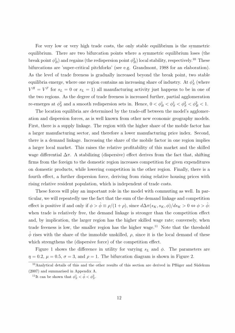
For very low or very high trade costs, the only stable equilibrium is the symmetric

equilibrium. There are two bifurcation points where a symmetric equilibrium loses (the

break point φ1B) and regains (the redispersion point φ2

B) local stability, respectively.10 These

bifurcations are ’super-critical pitchforks’ (see e.g. Grandmont, 1988 for an elaboration).

As the level of trade freeness is gradually increased beyond the break point, two stable

equilibria emerge, where one region contains an increasing share of industry. At φ1S (where

V H = V F for sL = 0 or sL = 1) all manufacturing activity just happens to be in one of

the two regions. As the degree of trade freeness is increased further, partial agglomeration

re-emerges at φ2S and a smooth redispersion sets in. Hence, 0 < φ1

B < φ1S < φ2

S < φ2B < 1.

The location equilibria are determined by the trade-off between the model’s agglomer-

ation and dispersion forces, as is well known from other new economic geography models.

First, there is a supply linkage. The region with the higher share of the mobile factor has

a larger manufacturing sector, and therefore a lower manufacturing price index. Second,

there is a demand linkage. Increasing the share of the mobile factor in one region implies

a larger local market. This raises the relative profitability of this market and the skilled

wage differential ∆π. A stabilizing (dispersive) effect derives from the fact that, shifting

firms from the foreign to the domestic region increases competition for given expenditures

on domestic products, while lowering competition in the other region. Finally, there is a

fourth effect, a further dispersion force, deriving from rising relative housing prices with

rising relative resident population, which is independent of trade costs.

These forces will play an important role in the model with commuting as well. In par-

ticular, we will repeatedly use the fact that the sum of the demand linkage and competition

effect is positive if and only if φ > φ ≡ ρ/(1 + ρ), since d∆π(sK , sK , φ)/dsK > 0 ⇔ φ > φ:

when trade is relatively free, the demand linkage is stronger than the competition effect

and, by implication, the larger region has the higher skilled wage rate; conversely, when

trade freeness is low, the smaller region has the higher wage.11 Note that the threshold

φ rises with the share of the immobile unskilled, ρ, since it is the local demand of these

which strengthens the (dispersive force) of the competition effect.

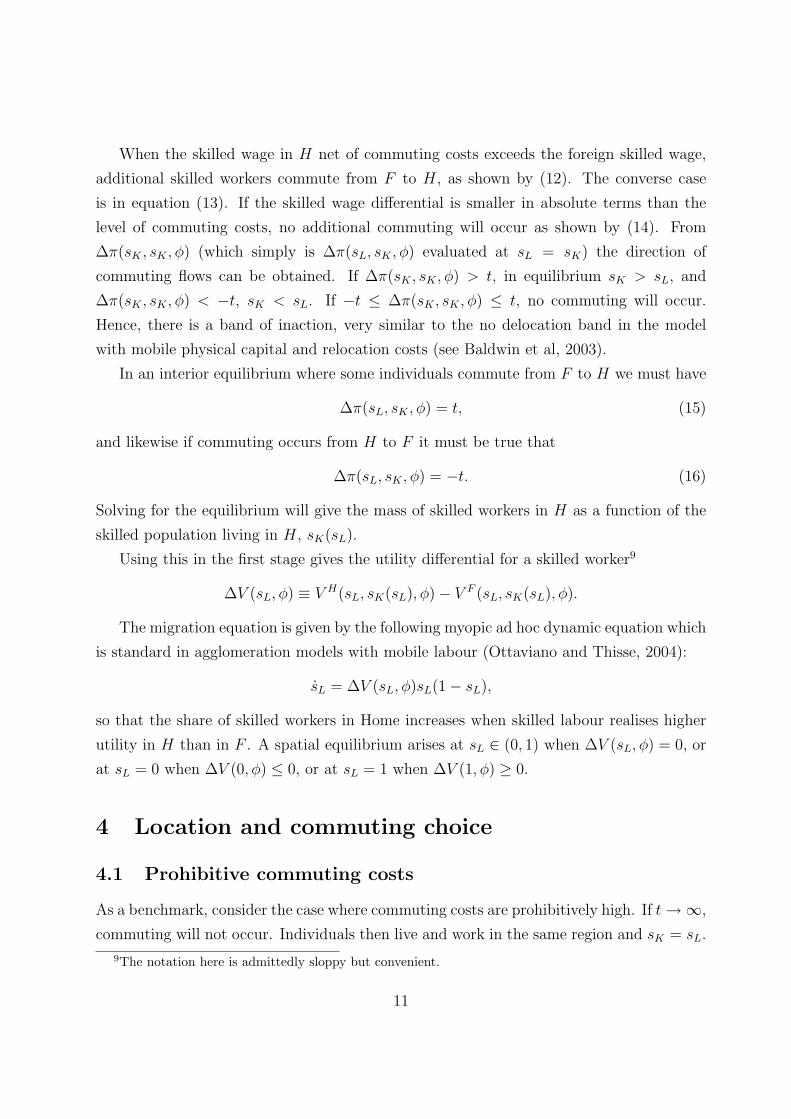
Figure 1 shows the difference in utility for varying sL and φ. The parameters are

η = 0.2, µ = 0.5, σ = 3, and ρ = 1. The bifurcation diagram is shown in Figure 2.

10Analytical details of this and the other results of this section are derived in Pfluger and Sudekum

(2007) and summarised in Appendix A.11It can be shown that φ1

S < φ < φ2S .

12

0.2 0.4 0.6 0.8 1

-0.02

-0.01

0.01

0.02

sL

ΔV

φ high/low

φ very high/low

φ intermediate

Figure 1: ∆V without long-distance commuting

0 0.4 10

0.2

0.4

0.6

0.8

1

φ

sL

0

0.2

0.4

0.6

0.8

1

φ1B φ2Bφ1S φ2Sφ

Figure 2: Bifurcation diagram without long-distance commuting

13

4.2 Equilibrium with zero commuting costs

We are now interested in how location equilibria are affected by the possibility of commut-

ing. If individuals commute in equilibrium, we have to distinguish between agglomeration

of jobs and agglomeration of residences. We will proceed by first describing in detail the

commuting equilibrium, i.e., for given residence choice we identify the pattern of commut-

ing.

We note again that in the alternative interpretation of the model with capital mobility,

commuting should be replaced by capital flows. Capital would then flow from the low-rent

to the high-rent region, with the direction of net capital flows depending on trade freeness,

as shown below for the case of commuting.

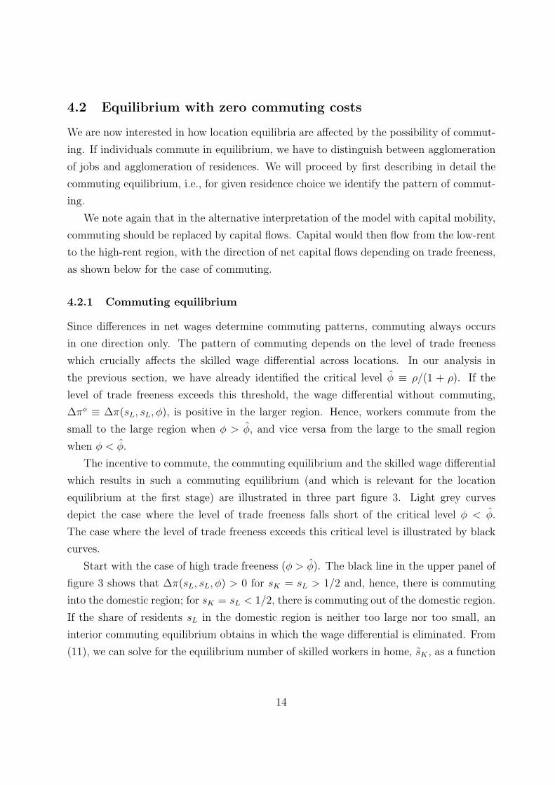
4.2.1 Commuting equilibrium

Since differences in net wages determine commuting patterns, commuting always occurs

in one direction only. The pattern of commuting depends on the level of trade freeness

which crucially affects the skilled wage differential across locations. In our analysis in

the previous section, we have already identified the critical level φ ≡ ρ/(1 + ρ). If the

level of trade freeness exceeds this threshold, the wage differential without commuting,

∆πo ≡ ∆π(sL, sL, φ), is positive in the larger region. Hence, workers commute from the

small to the large region when φ > φ, and vice versa from the large to the small region

when φ < φ.

The incentive to commute, the commuting equilibrium and the skilled wage differential

which results in such a commuting equilibrium (and which is relevant for the location

equilibrium at the first stage) are illustrated in three part figure 3. Light grey curves

depict the case where the level of trade freeness falls short of the critical level φ < φ.

The case where the level of trade freeness exceeds this critical level is illustrated by black

curves.

Start with the case of high trade freeness (φ > φ). The black line in the upper panel of

figure 3 shows that ∆π(sL, sL, φ) > 0 for sK = sL > 1/2 and, hence, there is commuting

into the domestic region; for sK = sL < 1/2, there is commuting out of the domestic region.

If the share of residents sL in the domestic region is neither too large nor too small, an

interior commuting equilibrium obtains in which the wage differential is eliminated. From

(11), we can solve for the equilibrium number of skilled workers in home, sK , as a function

14

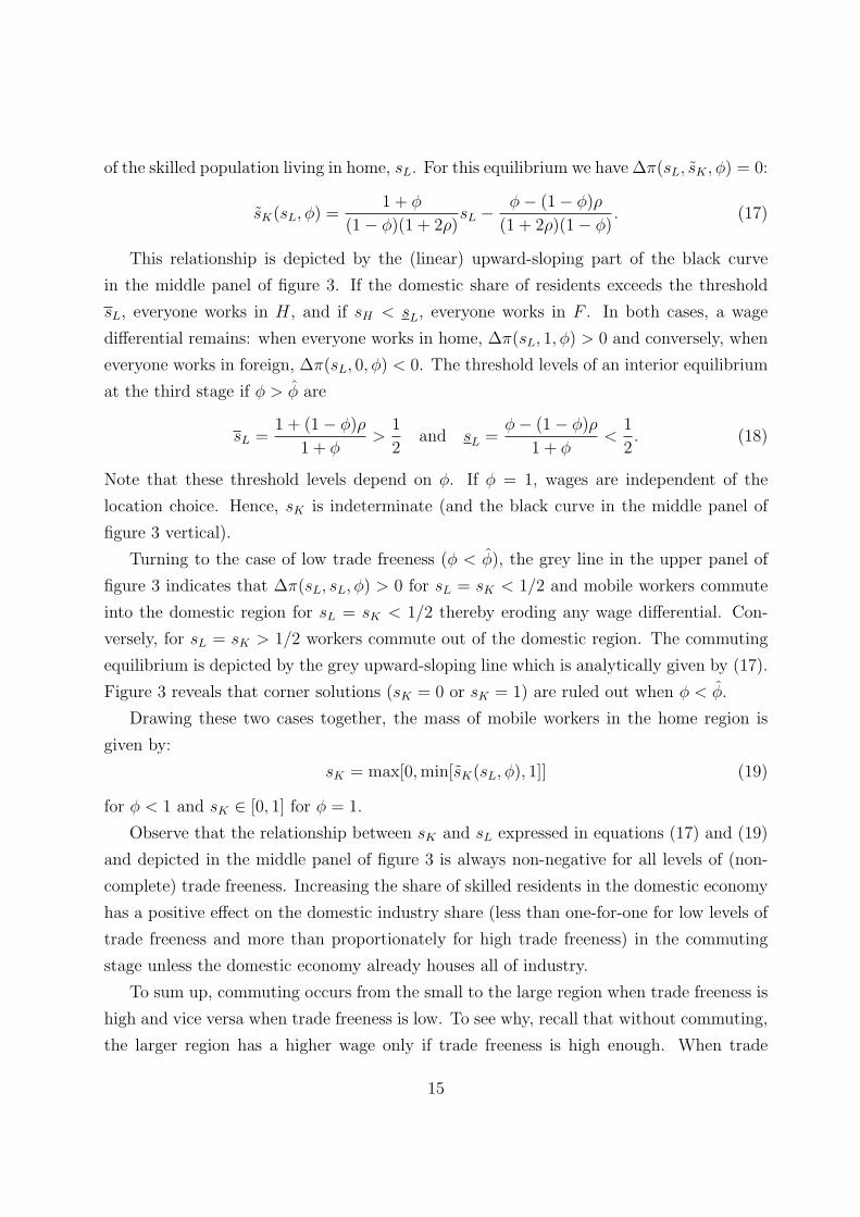
of the skilled population living in home, sL. For this equilibrium we have ∆π(sL, sK , φ) = 0:

sK(sL, φ) =1 + φ

(1− φ)(1 + 2ρ)sL −

φ− (1− φ)ρ

(1 + 2ρ)(1− φ). (17)

This relationship is depicted by the (linear) upward-sloping part of the black curve

in the middle panel of figure 3. If the domestic share of residents exceeds the threshold

sL, everyone works in H, and if sH < sL, everyone works in F . In both cases, a wage

differential remains: when everyone works in home, ∆π(sL, 1, φ) > 0 and conversely, when

everyone works in foreign, ∆π(sL, 0, φ) < 0. The threshold levels of an interior equilibrium

at the third stage if φ > φ are

sL =1 + (1− φ)ρ

1 + φ>

1

2and sL =

φ− (1− φ)ρ

1 + φ<

1

2. (18)

Note that these threshold levels depend on φ. If φ = 1, wages are independent of the

location choice. Hence, sK is indeterminate (and the black curve in the middle panel of

figure 3 vertical).

Turning to the case of low trade freeness (φ < φ), the grey line in the upper panel of

figure 3 indicates that ∆π(sL, sL, φ) > 0 for sL = sK < 1/2 and mobile workers commute

into the domestic region for sL = sK < 1/2 thereby eroding any wage differential. Con-

versely, for sL = sK > 1/2 workers commute out of the domestic region. The commuting

equilibrium is depicted by the grey upward-sloping line which is analytically given by (17).

Figure 3 reveals that corner solutions (sK = 0 or sK = 1) are ruled out when φ < φ.

Drawing these two cases together, the mass of mobile workers in the home region is

given by:

sK = max[0, min[sK(sL, φ), 1]] (19)

for φ < 1 and sK ∈ [0, 1] for φ = 1.

Observe that the relationship between sK and sL expressed in equations (17) and (19)

and depicted in the middle panel of figure 3 is always non-negative for all levels of (non-

complete) trade freeness. Increasing the share of skilled residents in the domestic economy

has a positive effect on the domestic industry share (less than one-for-one for low levels of

trade freeness and more than proportionately for high trade freeness) in the commuting

stage unless the domestic economy already houses all of industry.

To sum up, commuting occurs from the small to the large region when trade freeness is

high and vice versa when trade freeness is low. To see why, recall that without commuting,

the larger region has a higher wage only if trade freeness is high enough. When trade

15

00.5

sL

Δπ(sL)

0 1sL

sK

1

0.5

1

φ''>φ^φ'<φ^

sL-sL-

φ'<φ^φ''>φ^

00.5

sL

ΔV(sL)

1

φ''>φ^

φ'<φ^

sL

sL- sL-

Figure 3: Commuting pattern with t = 0

16

freeness is less than φ, wages are higher in the small region. Intuitively, although the

larger region has a larger market, this effect is swamped by the fact that high trade costs

reduce demand by the consumers of the small region. Therefore, firms have an incentive

to serve the local market in the small region. With low enough trade freeness, this effect

dominates the home market effect and, therefore, the smaller region will have higher skilled

wages (see Krugman, 1991). Commuting therefore occurs from the large to the small region

when trade is sufficiently closed.

4.2.2 Location equilibrium

Ultimately, we are interested in the effect of commuting on the location of residences.

Therefore, we now describe the effect of commuting on the location equilibrium. In par-

ticular, we ask whether commuting leads to more or less agglomeration of residences than

what we find in a world without long-distance commuting.

Let us rewrite the utility of an individual choosing to live in H as

V H = max{πH , πF} − µ ln PH − η ln QH . (20)

An analogous expression holds for an individual choosing to live in F . Equation (20) shows

that the choice of residence will affect the price level of manufactured goods and the price

of housing but not the wage, since costless commuting means individuals will work in the

high-wage region regardless of their residence.

Therefore, the utility difference of a resident between living at home or in foreign can

be written as:

∆V (sL, φ) = µ ln

(P F

PH

)+ η ln

(QF

QH

)(21)

=µ

1− σln

(1− sK + φsK

sK + φ(1− sK)

)+ η ln

(ρ + 1− sL

ρ + sL

). (22)

with sK = sK(sL, φ) given by (19). The first term on the right of (21) shows the effect of

the difference in the price levels between the regions, and the second term shows the effect

of differences in housing prices. Again, note that the difference in wages disappears from

the utility differential (21), since commuting means individuals will earn the same wage

(namely, max{πH , πF}) regardless of their place of residence.

Commuting changes the utility difference and therefore migration incentives through

its effect on the price index of industrial goods (the housing market congestion does not

depend on the mass of commuters since by assumptions firms occupy no space).

17

Equation (21) shows the fundamental forces of agglomeration and dispersion in the

model with commuting. Since differences of profits have disappeared from this equation,

the usual demand linkage and competition effects of agglomeration running through the

differences in profits are no longer operative. We are therefore left with the differences

in housing prices and the supply linkage running through the price indices of industrial

goods.

Looking at relative housing prices first, from (22) we have

d ln(QF /QH)

dsL

= − 1 + 2ρ

(ρ + 1− sL)(ρ + sL)< 0. (23)

The housing market effect always deters agglomeration and is independent of trade free-

ness.12

Proceeding likewise, from (22) we find the effect of varying sL on relative manufacturing

prices. If φ = 1, consumer good prices are uniform across regions and independent of

industry locations and residence choices: P F /PH = 1. Otherwise:

d ln(P F /PH)

dsL

=d ln(P F /PH)

dsK

dsK

dsL

(24)

=−(1− φ2)

(1− σ)(1− sK + φsK)(sK + φ(1− sK))

dsK

dsL

. (25)

Using (17), we get for the interior commuting equilibrium:

d ln(P F /PH)

dsL

= − (1 + 2ρ)

(1− σ)(ρ + 1− sL)(ρ + sL)> 0 (26)

The cost-of-living effect would seem to depend on φ. As shown by (25), increasing the

number of firms in H lowers the relative price index in H and fall in relative prices is

decreasing in φ. However, this effect is just offset by the effect of a larger population

on the number of firms through commuting, as shown by (26): when φ is low, prices

decrease strongly with the number of firms but the number of firms increases less than

proportionately with population since commuting occurs from the large to the small region;

conversely with high φ prices decrease less with the number of firms but commuting implies

that the number of firms increases more than proportionately with population.

12This follows because of quasilinear utility which implies that the demand for housing does not depend

on income.

18

Indeed, in the interior commuting equilibrium, the price effect is independent of the

degree of trade freeness and (21) simplifies to

∆V (sL, φ) =

(µ

1− σ+ η

)ln

(ρ + 1− sL

ρ + sL

). (27)

Hence, we get

d (∆V (sL, φ))

dsL

= −(

µ

1− σ+ η

)1 + 2ρ

(ρ + 1− sL)(ρ + sL)> 0, (28)

where the inequality follows from a parameter restriction to restrict the congestion force

associated with the housing sector – otherwise, symmetry would be the only equilibrium

and commuting would therefore never occur (see Appendix A).

Interestingly, we find that the utility differential ∆V slopes upward in the interior

commuting equilibrium regardless of the level of trade freeness (below φ = 1). Since this

holds, in particular, at the symmetric allocation sL = 1/2, we have:

Proposition 1 When commuting costs are zero, a symmetric equilibrium is always unsta-

ble provided that trade costs are positive.

The lower panel of Figure 3 shows the utility differential and location equilibria with

commuting for small and large φ.13 Symmetry (sL = 1/2, and, therefore, sK = 1/2) is

always an equilibrium, i.e. V H(1/2, φ) = V F (1/2, φ). This location equilibrium is unstable

for all non-zero levels of trade freeness, however, as we have just shown.

An interior commuting equilibrium always obtains for φ < φ. Hence, the utility dif-

ference ∆V slopes upwards for all values sL ∈ [0, 1]. The grey line depicts this case and

reveals that we have a unique unstable symmetric equilibrium and two stable equilibria

with full agglomeration of residences.

An interior commuting equilibrium also obtains for 1 > φ > φ as long as sL ≤ sL ≤ sL

(recall that sK ∈ (0, 1) in this case). Hence, as depicted by the black line, the utility

difference must also slope upwards in the vicinity of the symmetric equilibrium. However,

at the point where everyone works in, say, H, an increase in the resident population has

no more effect on the working population (this corresponds to sL > sL in the lower panel

in Figure 3).

13∆V ist strictly concave for sL ∈ (0, 1/2) and strictly convex for sL ∈ (1/2, 1). For our set of parameters,

the curve is close to linear.

19

Setting sK = 1 in (21) and differentiating for φ < 1 w.r.t. sL gives:

d∆V (sL, φ)

dsL

∣∣∣∣sL>sL

= − η(1 + 2ρ)

(ρ + sL)(ρ + 1− sL)< 0. (29)

Hence, the ∆V curve has a kink at sL and slopes downward for sL > sL. As φ gets

larger, the utility differential must eventually get negative for large sL when trade is almost

completely free. This is intuitive since when trade is completely free, location plays no

role for the agglomeration of firms and the prices of industrial goods. The only effect of

increasing population is then increased congestion in the housing market, which implies

that as φ → 1, ∆V must be negative at sL = 1.

Hence, we can conclude that with sufficiently free trade a stable equilibrium with a

partial agglomeration of residences emerges. By analogous reasoning, the same holds true

at the point when everyone works in F .

Lemma 1 (i) There exists a level of trade freeness φ, with φ > φ, such that ∆V (1, φ) = 0.

(ii) For 1 > φ > φ and sL > 1/2 (sL < 1/2), there exists a unique sL, with sL < 1 (sL > 0),

such that ∆V (sL, φ) = 0 and d∆V (sL, φ)/dsL < 0. (iii) Furthermore, ∆V (1/2, 1) = 0 and

d∆V (1/2, 1)/dsL < 0.

Proof. See Appendix B. �

Lemma 1 directly implies the following result:

Proposition 2 Suppose commuting costs are zero. Then, (i) if φ < φ, there exist an

unstable symmetric equilibrium and two stable equilibria with full agglomeration, one with

sL = 1 and one with sL = 0; (ii) if 1 > φ > φ > φ, there exist an unstable symmetric

equilibrium and two stable asymmetric equilibria with partial agglomeration of residences,

one with sL > 1/2 and one with sL < 1/2; (iii) if φ = 1, there exists a unique stable

symmetric equilibrium.

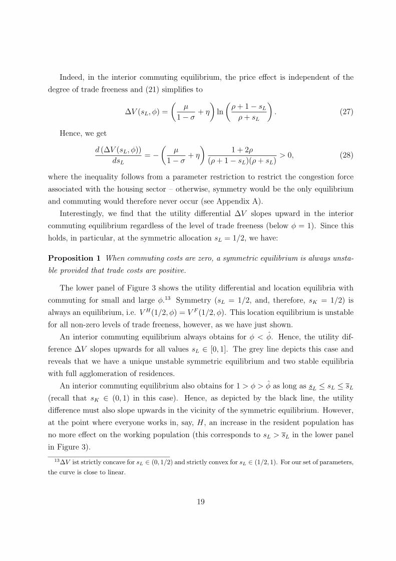
Figure 4 shows the bifurcation diagram, comparing the case of zero commuting costs

(dark lines) with the case of prohibitive costs (light lines).

Proposition 2 together with (19) implies the following for the location of industry:

Corollary 1 With zero commuting costs, when φ < φ, there is partial agglomeration of

firms, with either 1/2 < sK < 1 or 1/2 > sK > 0; and when 1 > φ ≥ φ, there is complete

agglomeration of firms with either sK = 1 or sK = 0.

20

0 10

0.2

0.4

0.6

0.8

1

φ

sL

0

0.2

0.4

0.6

0.8

1

φ1B φ2Bφ1S φ2,oSφ0.2 φ2,cS

Figure 4: Bifurcation diagram with zero commuting costs

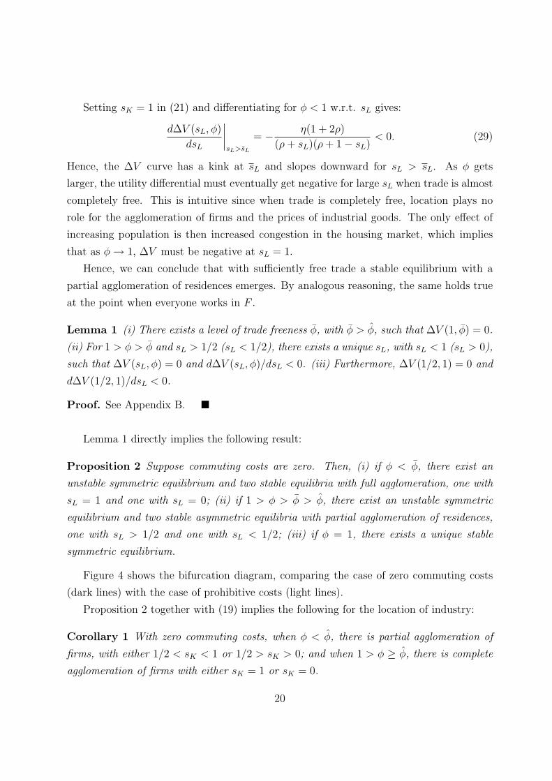
The bifurcation diagram for the location of industry with and without commuting is

shown in Figure 5. Comparison with Figure 4 shows that there is an interesting contrast

between agglomeration of residences and industry: while residences are agglomerated when

trade is closed and dispersed when trade is free, conversely, industry is dispersed when trade

is closed and agglomerated when trade is free. This reflects the workings of the fundamental

agglomeration forces: the location of industry is governed solely by the wage differential.

When trade is free (namely φ > φ), wages are higher in the larger region and there is

commuting from the small to the large region. Conversely, with relatively closed trade,

wages are higher in the smaller region and commuting occurs from the large to the small

region, i.e. industry is dispersed.

It is instructive, again, to look at the intuition for the diverging agglomeration of jobs

and residences. Suppose that trade is closed. Then, for given residence locations, workers

commute from the large to the small region, since the dominance of the competition effect

ensures that wages are higher in the smaller region, as shown in the previous subsection.

This implies that full agglomeration of jobs cannot be an equilibrium. However, the supply

linkage dominates the congestion effect of the housing market so that full agglomeration

of residences obtains while jobs are only partially agglomerated.

On the other hand, when trade is sufficiently free, the demand linkage dominates the

21

0 0.4 10

0.2

0.4

0.6

0.8

1

φ

sK

0

0.2

0.4

0.6

0.8

1

φ1B φ2Bφ1S φ2Sφ

Figure 5: Bifurcation diagram (sK)

competition effect so we will get agglomeration of jobs in the region with the larger pop-

ulation. When jobs are fully agglomerated in, say, region H, a symmetric allocation of

residences is unstable. However, an increase in the resident population now reduces the

utility differential between the large and small region, since with all jobs already in H, the

only effect of increasing population is to increase congestion in housing markets. Hence,

for sufficiently large φ, we get stable equilibria with partial agglomeration of residences

and full agglomeration of jobs.

Turning back to the location of residences, Figure 4 shows that for φ < φ, we have

unambiguously more agglomeration (of residences) with than without commuting. This is

immediately clear, since only full agglomeration can be a stable equilibrium in this case.

For 1 > φ > φ, we find more agglomeration with commuting when trade is sufficiently

free. However, we find that with commuting, partial agglomeration emerges at lower

trade freeness than without commuting. Hence, the effect of commuting on agglomeration

depends on the level of trade freeness.

We prove in the Appendix that (a) the ‘sustain’ point φ2S – i.e., the point where we have

full agglomeration of residences (and jobs) in H – is lower with than without commuting,14

14The intuition is as follows: the sustain point with commuting equalises the dispersion force of the

housing sector with the agglomeration force of the cost-of-living effect evaluated at sL = 1. Without

22

while (b) in the commuting case the ‘break’ point φ2B – i.e., the point where the symmetric

equilibrium becomes unstable – equals one and thus exceeds the corresponding point in

the no-commuting case. The indices c, o here refer to the equilibrium with and without

commuting respectively.

Lemma 2 We have φ < φ2,oS < φ2,c

S < φ2,oB < φ2,c

B = 1.

Proof. See Appendix B. �

Lemma 2 obviuosly implies that there exists a φ ∈ [φ2,cS , φ2,o

B ] such that for all φ2,cS <

φ < φ, we have sP,cL < sP,o

L . Therefore, we have shown the following:

Proposition 3 Comparing commuting and no-commuting equilibria, we have more ag-

glomeration of residences in the commuting case when trade freeness is low or high, while

there is less agglomeration for intermediate trade freeness, that is, scL ≤ so

L for all φ ∈[φ2,c

S , φ] and scL ≥ so

L for φ < φ2,cS and φ ≥ φ2,o

B .

Note that from the ranking of the ‘break’ and ‘sustain’ points and the fact that the

locus of partial agglomeration equilibria is concave with prohibitive commuting costs and

convex with zero commuting costs (see Figure 4), we should be able to infer that there

is more agglomeration of residences in the zero commuting cost case when φ is outside

the interval φ ∈ [φ2,cS , φ]. Numerical simulations show that there exists a wide range of

parameters such that this is indeed the case. Summarising this discussion, we have:

Result 1 Suppose commuting costs are zero. Then, there is more agglomeration of resi-

dences than with prohibitive commuting costs except for intermediate levels of trade free-

ness, i.e., φ ∈ [φ2,cS , φ].

4.3 Equilibrium with positive commuting costs

We now analyse the case of positive commuting costs, proceeding like we did in the last

subsection. However, since the algebra of the case with positive commuting costs is more

involved, our main result rely on graphical representations and numerical simulations in-

stead.

commuting, these two forces have the same strength (since sK = sL = 1) but, since φ2,cS > φ, nominal

wages are higher in H than in F when sL = 1. Therefore, ∆V o(1, φ2,cS ) > 0.

23

4.3.1 Commuting equilibrium

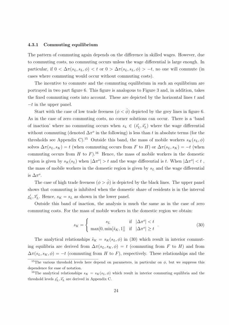
The pattern of commuting again depends on the difference in skilled wages. However, due

to commuting costs, no commuting occurs unless the wage differential is large enough. In

particular, if 0 < ∆π(sL, sL, φ) < t or 0 > ∆π(sL, sL, φ) > −t, no one will commute (in

cases where commuting would occur without commuting costs).

The incentive to commute and the commuting equilibrium in such an equilibrium are

portrayed in two part figure 6. This figure is analogous to Figure 3 and, in addition, takes

the fixed commuting costs into account. These are depicted by the horizontal lines t and

−t in the upper panel.

Start with the case of low trade freeness (φ < φ) depicted by the grey lines in figure 6.

As in the case of zero commuting costs, no corner solutions can occur. There is a ‘band

of inaction’ where no commuting occurs when sL ∈ (s′L, s′L) where the wage differential

without commuting (denoted ∆πo in the following) is less than t in absolute terms (for the

thresholds see Appendix C).15 Outside this band, the mass of mobile workers sK(sL, φ)

solves ∆π(sL, sK) = t (when commuting occurs from F to H) or ∆π(sL, sK) = −t (when

commuting occurs from H to F ).16 Hence, the mass of mobile workers in the domestic

region is given by sK(sL) when |∆πo| > t and the wage differential is t. When |∆πo| < t ,

the mass of mobile workers in the domestic region is given by sL and the wage differential

is ∆πo.

The case of high trade freeness (φ > φ) is depicted by the black lines. The upper panel

shows that commuting is inhibited when the domestic share of residents is in the interval

s′L, s′L. Hence, sK = sL as shown in the lower panel.

Outside this band of inaction, the analysis is much the same as in the case of zero

commuting costs. For the mass of mobile workers in the domestic region we obtain:

sK =

{sL if |∆πo| < t

max[0, min[sK , 1]] if |∆πo| ≥ t. (30)

The analytical relationships sK = sK(sL, φ) in (30) which result in interior commut-

ing equilibria are derived from ∆π(sL, sK , φ) = t (commuting from F to H) and from

∆π(sL, sK , φ) = −t (commuting from H to F ), respectively. These relationships and the

15The various threshold levels here depend on parameters, in particular on φ, but we suppress this

dependence for ease of notation.16The analytical relationships sK = sK(sL, φ) which result in interior commuting equilibria and the

threshold levels s′L, s′L are derived in Appendix C.

24

thresholds s′′L and s′′L which indicate the borderline values of the share of domestic residents

at which corner solutions obtain in the commuting equilibrium, are analytically stated in

Appendix C).

The skilled wage differential relevant for the residence choice (see below) corresponding

to the solution of the commuting equilibrium is:

∆π =

{∆πo if |∆πo| < t

sign[∆πo]t if |∆πo| ≥ t. (31)

Inside the band of inaction where |∆πo| < t the skilled wages correspond to their values

without commuting. Outside, the wage differential is equalised at t (when ∆π > 0) or

−t (when ∆π < 0). This holds for an interior equilibrium. Again, the relevant wage

differential also equals t or −t for a corner equilibrium: If everyone works in H (which

occurs when ∆π > 0), say, the wage obtained when living in H is πH and that when living

in F is πH − t, hence the differential t. Similarly, when everyone works in F (∆π < 0), the

wage differential is −t.

At an interior commuting equilibrium, increasing sL increases the share of firms at

home sK more than (less than) proportionately depending on whether φ > (<)φ.

This completes our discussion of the equilibrium at the commuting stage.

4.3.2 Location equilibrium

As in the previous subsection, we analyse the effect of commuting on the utility differential

of skilled workers. The utility differential which guides the location choice, takes the skilled

wage differential and the equilibrium share of firms sK(sL, φ) in the commuting equilibrium

into account (i.e. (30)). We now have:

∆V (sL, φ) =µ

1− σln

(1− sK + φsK

sK + φ(1− sK)

)+ η ln

(ρ + 1− sL

ρ + sL

)+ sign[∆πo] min{|∆πo|, t},

(32)

where sK = sK(sL) is given by equations (A.4) and (A.8) of Appendix C for the interior

solution.

From the analysis of the second stage around sL = 1/2 we know that, due to the

presence of commuting costs, no commuting occurs (i.e. sK = sL) and the skilled wage

differential is the same as with prohibitive commuting costs for all levels of trade free-

ness. Hence, long-distance commuting has no effect on the local stability of the symmetric

25

00.5

sL

Δπ(sL)

0 1sL

sK

1

0.5

1

φ''>φ^φ'<φt

-t

s'L

^

s''L- s''L-

s''L

^

φ'<φ^

φ''>φ^

s'L^s''L^

Figure 6: Commuting with t > 0

26

sL

ΔV

0.45 0.5 0.55 0.6

-0.03

-0.02

-0.01

0.01

0.02

0.03

Figure 7: ∆V with t > 0 and φ < φ1B.

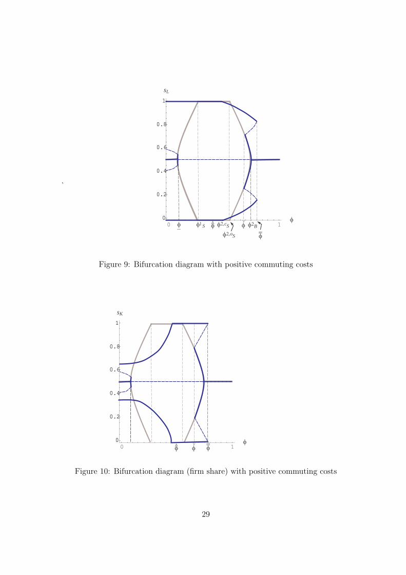
equilibrium. This is depicted in figure 9, which superimposes the bifurcation diagram with

positive commuting costs on the bifurcation diagram with prohibitive commuting costs (i.e.

figure 2). This implies, of course, that the symmetric equilibrium is stable with commuting

if and only if it is stable without commuting.

To explore the stability characteristics of other possible equilibria, we have to analyse

the utility differential when we are outside the band on inaction. As we know from the

commuting stage, the degree of trade freeness now matters.

Start with low levels of trade freeness, i.e. φ < φ. For sL 6∈ (s′L, s′L), an interior

equilibrium must obtain, i.e., we have to take into account that sK = sK(sL, φ) as given

by (30). By the same argument as in the previous subsection, when sK = sK , it can be

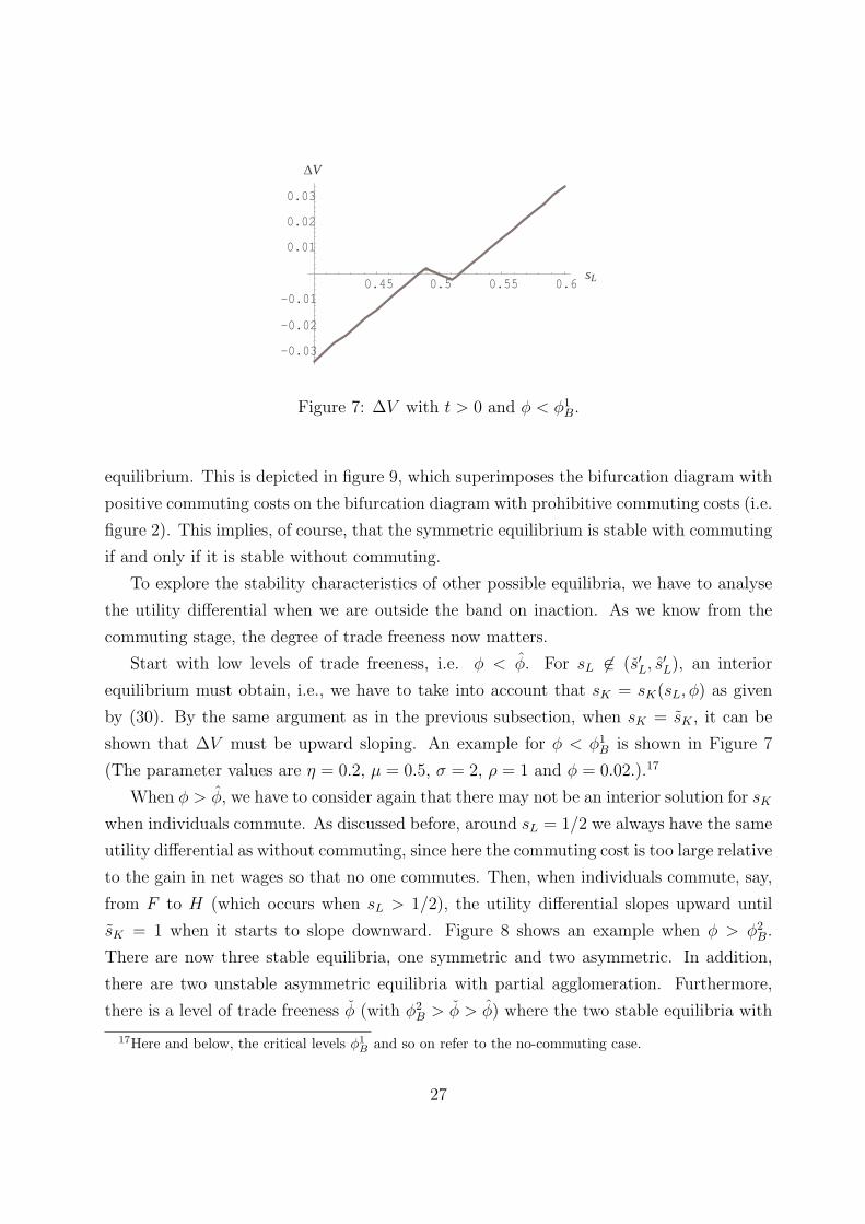
shown that ∆V must be upward sloping. An example for φ < φ1B is shown in Figure 7

(The parameter values are η = 0.2, µ = 0.5, σ = 2, ρ = 1 and φ = 0.02.).17

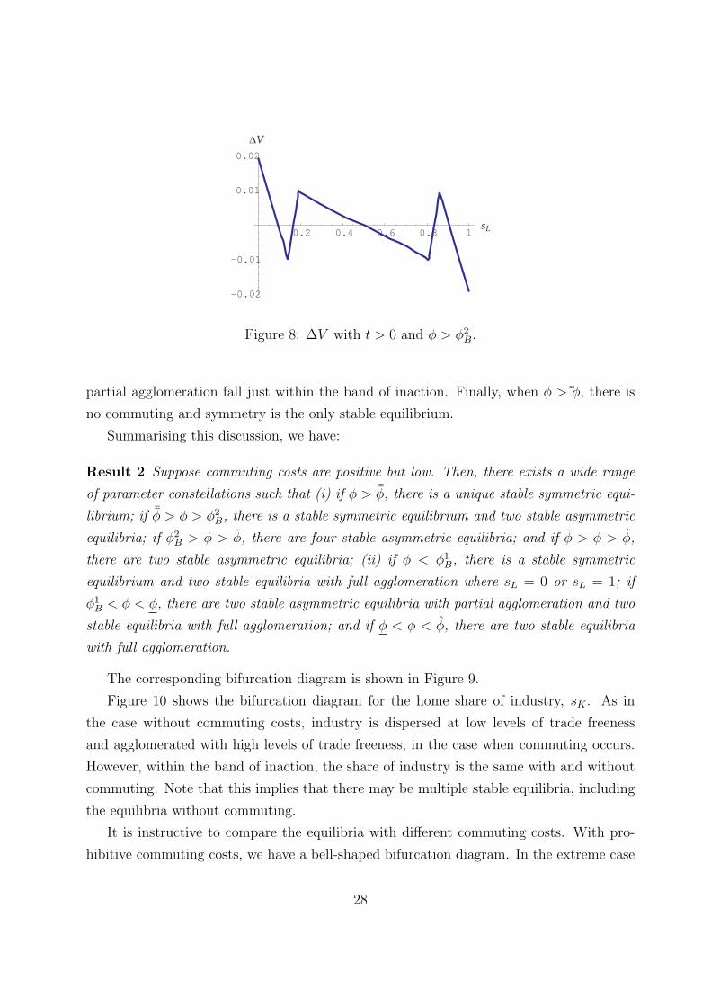
When φ > φ, we have to consider again that there may not be an interior solution for sK

when individuals commute. As discussed before, around sL = 1/2 we always have the same

utility differential as without commuting, since here the commuting cost is too large relative

to the gain in net wages so that no one commutes. Then, when individuals commute, say,

from F to H (which occurs when sL > 1/2), the utility differential slopes upward until

sK = 1 when it starts to slope downward. Figure 8 shows an example when φ > φ2B.

There are now three stable equilibria, one symmetric and two asymmetric. In addition,

there are two unstable asymmetric equilibria with partial agglomeration. Furthermore,

there is a level of trade freeness φ (with φ2B > φ > φ) where the two stable equilibria with

17Here and below, the critical levels φ1B and so on refer to the no-commuting case.

27

sL

ΔV

0.2 0.4 0.6 0.8 1

-0.02

-0.01

0.01

0.02

Figure 8: ∆V with t > 0 and φ > φ2B.

partial agglomeration fall just within the band of inaction. Finally, when φ > ¯φ, there is

no commuting and symmetry is the only stable equilibrium.

Summarising this discussion, we have:

Result 2 Suppose commuting costs are positive but low. Then, there exists a wide range

of parameter constellations such that (i) if φ > ¯φ, there is a unique stable symmetric equi-

librium; if ¯φ > φ > φ2B, there is a stable symmetric equilibrium and two stable asymmetric

equilibria; if φ2B > φ > φ, there are four stable asymmetric equilibria; and if φ > φ > φ,

there are two stable asymmetric equilibria; (ii) if φ < φ1B, there is a stable symmetric

equilibrium and two stable equilibria with full agglomeration where sL = 0 or sL = 1; if

φ1B < φ < φ, there are two stable asymmetric equilibria with partial agglomeration and two

stable equilibria with full agglomeration; and if φ < φ < φ, there are two stable equilibria

with full agglomeration.

The corresponding bifurcation diagram is shown in Figure 9.

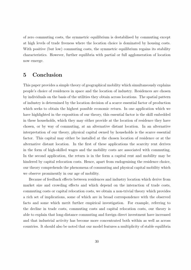
Figure 10 shows the bifurcation diagram for the home share of industry, sK . As in

the case without commuting costs, industry is dispersed at low levels of trade freeness

and agglomerated with high levels of trade freeness, in the case when commuting occurs.

However, within the band of inaction, the share of industry is the same with and without

commuting. Note that this implies that there may be multiple stable equilibria, including

the equilibria without commuting.

It is instructive to compare the equilibria with different commuting costs. With pro-

hibitive commuting costs, we have a bell-shaped bifurcation diagram. In the extreme case

28

0 10

0.2

0.4

0.6

0.8

1

φ

sL

0

0.2

0.4

0.6

0.8

1

φ φ2Bφ1S φ2,cSφ φ

^

φ−−φ2,oS

_

Figure 9: Bifurcation diagram with positive commuting costs

0 10

0.2

0.4

0.6

0.8

1

φ

sK

0

0.2

0.4

0.6

0.8

1

φ φ−−φ

^

Figure 10: Bifurcation diagram (firm share) with positive commuting costs

29

of zero commuting costs, the symmetric equilibrium is destabilised by commuting except

at high levels of trade freeness where the location choice is dominated by housing costs.

With positive (but low) commuting costs, the symmetric equilibrium regains its stability

characteristics. However, further equilibria with partial or full agglomeration of location

now emerge.

5 Conclusion

This paper provides a simple theory of geographical mobility which simultaneously explains

people’s choice of residences in space and the location of industry. Residences are chosen

by individuals on the basis of the utilities they obtain across locations. The spatial pattern

of industry is determined by the location decision of a scarce essential factor of production

which seeks to obtain the highest possible economic return. In one application which we

have highlighted in the exposition of our theory, this essential factor is the skill embedded

in these households, which they may either provide at the location of residence they have

chosen, or by way of commuting, at an alternative distant location. In an alternative

interpretation of our theory, physical capital owned by households is the scarce essential

factor. This capital may either be installed at the chosen location of residence or at the

alternative distant location. In the first of these applications the scarcity rent derives

in the form of high-skilled wages and the mobility costs are associated with commuting.

In the second application, the return is in the form a capital rent and mobility may be

hindered by capital relocation costs. Hence, apart from endogenising the residence choice,

our theory comprehends the phenomena of commuting and physical capital mobility which

we observe prominently in our age of mobility.

Because of feedback effects between residences and industry location which derive from

market size and crowding effects and which depend on the interaction of trade costs,

commuting costs or capital relocation costs, we obtain a non-trivial theory which provides

a rich set of implications, some of which are in broad correspondence with the observed

facts and some which merit further empirical investigation. For example, referring to

the decline in trade costs, commuting costs and capital relocation costs, our theory is

able to explain that long-distance commuting and foreign direct investment have increased

and that industrial activity has become more concentrated both within as well as across

countries. It should also be noted that our model features a multiplicity of stable equilibria

30

when commuting costs or capital relocation costs are nonzero (but not so large as to prohibit

movement). Due to a band of inaction created by these mobility costs, another prediction

of our analysis is that dispersion of residences and industry is stable at low and high trade

costs.

As in all new economic geography models, our results are driven by some particular

assumptions concerning preferences, technologies and mobility costs. We believe, however,

that our analysis, in making use of the agglomeration and dispersion forces that obtain

across a wide variety of new economic geography models, is a useful starting place for

analysing the joint determination of industry location and residence choices.

Appendix

A The model without commuting

Here we briefly present some parameter restrictions taken from Pfluger and Sudekum

(2007). In order to obtain two real bifurcation levels, 1 + 4σ(σ − 1)[1 − γ(σ − 1)] > 0

has to be fulfilled, where γ = η/µ. A sufficient condition to fulfill this requirement which

we assume to hold is 1− γ(σ − 1) > 0. In order to rule out that the agglomerative forces

become so strong that the symmetric equilibrium is unstable even at infinite trade costs,

[ρ/(ρ−1)−2ρ](2ρ+1)/σ < γ has to be satisfied (no-black-hole condition). A sufficient con-

dition is 2ρ > σ/(σ−1). Both sectors are only active after trade if ρσ/[(2ρ+1)(σ−1)] > µ.

B Zero commuting costs: Proofs

Proof of Lemma 1. (i) If φ = φ, ∆V (1, φ) > 0. For φ > φ and sL > sL,

∆V (sL, φ) =

(µ

1− σ

)ln(φ) + η ln

(ρ + 1− sL

ρ + sL

)+ ∆π(sL, 1).

If φ = 1, we get immediately

∆V (1, 1) = η ln

(ρ

1 + ρ

)< 0.

31

Since ∆V (1, φ) is continuous and decreasing in φ, there exists a unique φ > φ, such that

∆V (1, φ) = 0. (ii) Let φ > φ. Obviously, ∆V (sL, φ) > 0. Let sL > sL. ∆V (sL, φ) is

strictly concave. Hence, if φ > φ, there exists exactly one sL, with 1 > sL > sL, such

that ∆V (sL, φ) = 0. This sL fulfills d∆V (sL, φ)/dsL < 0. A similar argument holds true

for sL < 1/2. (iii) ∆V (sL, 1) = η ln(QF /QH

). The unique solution of ∆V (sL, 1) = 0 is

sL = 1/2, where d∆V (1/2, 1)/dsL < 0. �

Proof of Lemma 2. Note first that from the previous analysis, we know that the analogues

of φ1,oB and φ1,o

S do not exist, i.e., for φ < φ only full agglomeration is an equilibrium. Second,

for the ‘sustain points’ we find φ2,cS < φ2,o

S : From (17), we know sK(1, φ) = 1. From (21),

we have

∆V c(1, φ) =µ

1− σln φ + η ln φ. (A.1)

Setting ∆V c(1, φ) = 0 in (A.1) and solving gives

φ2,cS = φη(σ−1)/µ > φ. (A.2)

The difference

∆V o(1, φ)−∆V c(1, φ) =µ

σ(1− φ)

(1 + ρ− ρ

φ

)(A.3)

is positive at φ = φ2,cS since φ = φ2,c

S > φ (and thus sK(1, φ) = 1), which establishes that

φ2,oS > φ2,c

S .

Finally, the ‘break point’ φ2,oB solves d∆V (1/2, φ2,o

B )/dsL = 0. With commuting, the

symmetric equilibrium is never stable for φ < 1. At φ = 1, however, we have ∆V c(1, 1) =

∆V o(1, 1) = 0. �

C Positive commuting costs

From ∆π(sL, sK , φ) = −t, one obtains

sK =1

2− 1

2(1− φ)σt

{µ(1 + 2ρ)(1− φ)

−√

(1− φ)2µ2(1 + 2ρ)2 − 2µ(1− φ2)σ(1− 2sL)t + σ2t2(1 + φ)2

}. (A.4)

32

Setting sK equal to 0 and sL, respectively, yields

sL =µ(1− φ)[φ− (1− φ)ρ]− φσt

µ(1− φ2), (A.5)

s′′L =1

2+

1

2(1− φ)σt

{2µ[φ− (1− φ)ρ]

−√

4µ2[φ− (1− φ)ρ]2 + (1 + φ)2σ2t2}

, (A.6)

s′L =1

2+

1

2(1− φ)σt

{2µ[φ− (1− φ)ρ]

+√

4µ2[φ− (1− φ)ρ]2 + (1 + φ)2σ2t2}

. (A.7)

From ∆π(sL, sK , φ) = t, one obtains

sK =1

2+

1

2(1− φ)σt

{µ(1 + 2ρ)(1− φ)

−√

(1− φ)2µ2(1 + 2ρ)2 + 2µ(1− φ2)σ(1− 2sL)t + σ2t2(1 + φ)2

}. (A.8)

Setting sK equal to 1 and sL, respectively, yields

sL =µ(1− φ)[1 + (1− φ)ρ] + φσt

µ(1− φ2), (A.9)

s′′L =1

2− 1

2(1− φ)σt

{2µ[φ− (1− φ)ρ]

−√

4µ2[φ− (1− φ)ρ]2 + (1 + φ)2σ2t2}

, (A.10)

s′L =1

2− 1

2(1− φ)σt

{2µ[φ− (1− φ)ρ]

+√

4µ2[φ− (1− φ)ρ]2 + (1 + φ)2σ2t2}

. (A.11)

References

Baldwin, R., R. Forslid, P. Martin, G. Ottaviano and F. Robert-Nicoud (2003). Economic

geography and public policy. Princeton University Press, Princeton and Oxford.

33

Baldwin, R. and P. Martin (1999). Two waves of globalisation: Superficial similarities and

fundamental differences. In H.Siebert (ed.), Globalisation and Labour, ch. 1, pp 3-59,

Mohr, Tubingen.

Dixit, A. and J.E. Stiglitz (1977). Monopolistic competition and optimum product diver-

sity. American Economic Review 67, 297-308.

Faini, R., J. de Melo and K. F. Zimmermann, eds. (1999) Migration. The Controversies

and the Evidence. Cambridge University Press, Cambridge.

Forslid, R. and G. Ottaviano (2003). An analytically solvable core-periphery model. Journal

of Economic Geography 3, 229-240.

Friedman, T. (1999). The Lexus and the Olive Tree. Farrar, Straus and Giroux.

Friedman, T. (2006). The World is Flat. Updated and Expanded Version. Farrar, Straus

and Giroux.

Grandmont, J.-M. (1988). Non-linear difference equations, bifurcations and chaos: An

introduction. Lecture Notes no. 5, IMSSS Economics Lecture Note Series, Stanford,

CA.

Krugman, P. (1991). Increasing returns and economic geography. Journal of Political

Economy 99, 483-499.

Krugman, P and R. Livas Elizondo. (1995). Trade policy and the third world metropolis.

Journal of Development Economics 49, 137-150.

Martin, P. and C.A. Rogers (1995). Industrial location and public infrastructure. Journal

of International Economics 39, 335-351.

Matha, T. and L. Wintr (2007). Modelling commuting flows across bordering regions.

Mimeo. Forthcoming in Applied Economic Letters.

MKW (2001). Scientific report on the mobility of cross-border workers within the EEA.

Report for the European Commission, DG Employment and Social Affairs, MKW. Mu-

nich.

Murata, Y. and J.-F. Thisse (2005). A simple model of economic geography a la Helpman-

Tabuchi. Journal of Urban Economics 58, 137-155.

34

OECD (2000) Employment outlook 2000. OECD, Paris.

OECD (2005) Employment outlook 2005. OECD, Paris.

Ogura, L.M. (2005). Urban growth controls and intercity commuting. Journal of Urban

Economics 57, 371-390.

Ottaviano G. and J.-F. Thisse (2004). Agglomeration and economic geography. In: Hen-

derson, J.V. and J.-F. Thisse (Eds.). Handbook of Regional and Urban Economics vol.

4, Elsevier, Amsterdam, 2563-2608.

Pfluger, M. (2004). A simple, analytically solvable Chamberlinian agglomeration model.

Regional Science and Urban Economics 34, 565-573.

Pfluger, M. and J. Sudekum (2007). Integration, agglomeration and welfare. Forthcoming,

Journal of Urban Economics.

Statistisches Bundesamt (2005). Leben und Arbeiten in Deutschland: Ergebnisse des

Mikrozensus 2004. Statistisches Bundesamt, Wiesbaden.

Tabuchi, T. (1998). Urban agglomeration and dispersion: A synthesis of Alonso and

Krugman. Journal of Urban Econonomics 44, 333-351.

Tabuchi, T. and J.-F. Thisse (2005). Regional specialization, urban hierarchy and com-

muting costs. International Economic Review 47, 1259-1317.

Vermeulen, W. (2003). A model for Dutch commuting. CPB Report 2003/1.

35