YRJÖ RINTA-JOUPPI - Vaasan yliopisto · YRJÖ RINTA-JOUPPI Development of Offshore Wind Power Price Competitiveness Using a New Logistics Construct ... A/S, NORDEX A/S and Vestas

Y R J Ö R I N T A - J O U P P I

Development of Offshore Wind Power Price Competitiveness Using a New Logistics Construct

A C T A W A S A E N S I A

No. 117

Industrial Management 6

U N I V E R S I T A S W A S A E N S I S 2 0 0 3

Reviewers Professor Lars Landberg

Risö National Laboratory

Wind Energy Department

Building VEA–125

P.O. Box 49, Frederiksborgvej 399

DK–4000 Roskilde

Denmark

Professor Peter Lund

Helsinki University of Technology

Technical Physics and Mathematics Department

P.O. Box 2200, Rakentajanaukio 2 C

FIN–02015 TKK

Finland

ACTA WASAENSIA 3

FOREWORD

Several persons from the University of Vaasa made the theoretical part of this research

possible. First of all I would like to express my sincere thanks to the supervisor of this

thesis, Professor Josu Takala, for giving me this possibility. I have also got helpful

guidance during the research work from Professor Tauno Kekäle and Professor Timo

Vekara. Especially I must mention two pre-examiners of this thesis, Professors Peter

Lund and Lars Landberg and to them I like to express my deepest gratitude.

There are numerous persons in the case enterprises who made the empirical part of this

research possible. I would like to thank all of them for their valuable work. I would

especially like to thank colleagues in companies Prizztech Oy, Merinova Oy Innovest,

Asteka Oy, Kustannussalpa Osk. and Hollming Kankaanpään konepaja Oy.

Great help has been given by the wind turbine manufacturers Bonus A/S, NEGMicon

A/S, NORDEX A/S and Vestas A/S and specially the agents of these companies. The

Finnish Meteorological Institute gave data from fixed meteorological stations. I am very

grateful for the assistance which I have received.

Interesting discussions concerning floating and embedded pieces were held with Aimo

Torp and concerning offshore work with the company Alfonso Håkans. Many thanks to

them.

My deep appreciation also goes to designer Tarja Salo for her help in creating visual

expressions in this dissertation and to John Shepherd and Jaakko Raitakari for revising

the language of the manuscript.

Finally, I would like to thank my family and friends for their support.

Pori, March 2003

Yrjö Rinta-Jouppi

4 ACTA WASAENSIA

CONTENTS

FOREWORD ................................................................................................................................. 3

LIST OF FIGURES .................................................................................................................... 8

LIST OF TABLES .................................................................................................................. 10

LIST OF APPENDICES.............................................................................................................. 12

ABSTRACT................................................................................................................................. 13

1. INTRODUCTION ............................................................................................................. 14

1.1 Background ............................................................................................................. 14

1.2 Research Problems and Objectives of the Study..................................................... 17

1.3 Research Strategy .................................................................................................... 19

1.4 Scope of the Study................................................................................................... 20

1.5 Research Approach and Methodology .................................................................... 21

1.6 Research Structure................................................................................................... 23

1.7 Summary ................................................................................................................. 24

2. THEORETICAL FRAMEWORK..................................................................................... 25

2.1 Differentiation into Environment Friendly Energy ................................................. 25

2.2 Growth and Market Share Matrix ........................................................................... 28

2.3 Natural Science........................................................................................................ 30

2.3.1 What is Wind?.......................................................................................... 30

2.3.2 The Height Effect..................................................................................... 33

2.3.3 Energy in the Wind .................................................................................. 38

2.4 Wind Energy Economics......................................................................................... 41

2.4.1 What does a Wind Turbine Cost? ............................................................ 43

2.4.2 Installation Costs for Wind Turbines....................................................... 44

2.4.3 Operation and Maintenance Costs for Wind Turbines ............................ 45

2.4.4 Income from Wind Turbines.................................................................... 47

2.4.5 Wind Energy and Electrical Tariffs ......................................................... 48

2.4.6 Basic Economies of Investment............................................................... 49

2.4.7 Wind Energy Economics ......................................................................... 51

2.4.8 Economics of Offshore Wind Energy...................................................... 52

2.4.9 Employment in the Wind Industry........................................................... 54

2.5 Offshore Wind Power.............................................................................................. 55

2.5.1 Offshore Wind Power in Europe.............................................................. 56

2.5.2 Experience from Realised Offshore Wind Power Projects...................... 56

ACTA WASAENSIA 5

2.5.3 Building of large Wind Power Parks ...................................................... 58

2.6 Offshore Foundation Technique.............................................................................. 60

2.6.1 Offshore Constructs in Ice Conditions..................................................... 60

2.6.2 Wind Power Plant Foundation on the Sea ............................................... 64

2.6.3 Caissons in the Tunö Knob Wind Park, Denmark................................... 65

2.6.4 Mono Piles ............................................................................................... 66

2.6.5 Construction Technology......................................................................... 69

2.6.6 Costs of Offshore Wind Power Plant....................................................... 71

2.6.7 Cost Estimation of Wind power Project .................................................. 73

2.6.8 Project Size and Water Depth Effect on the Costs .................................. 76

2.6.9 Spreadsheet computation simulation model for steel foundation. ........... 79

2.7 Wind Power Costs Calculation Model .................................................................... 81

2.7.1 Cost Components and Energy Production ............................................... 81

2.7.2 Cost Calculation Methodology, General Approach................................. 83

2.7.3 Cost Calculation Methodology, Simplified Approach............................. 84

2.7.4 Calculation Method.................................................................................. 84

2.8 Estimation and Specification of Input Parameters .................................................. 86

2.8.1 Investment................................................................................................ 86

2.8.2 Operation & Maintenance........................................................................ 87

2.8.3 Social Costs.............................................................................................. 88

2.8.4 Retrofit cost.............................................................................................. 89

2.8.5 Salvage value ........................................................................................... 89

2.8.6 Economic Lifetime................................................................................... 89

2.8.7 Discount Rate........................................................................................... 90

2.8.8 Wind Energy output ................................................................................. 91

2.8.9 Potential Energy Output........................................................................... 91

2.8.10 Wind Turbine Performance Factor .......................................................... 92

2.8.11 Site Factor ................................................................................................ 93

2.8.12 Technical Availability Factor .................................................................. 93

2.8.13 Net Energy Output ................................................................................... 94

2.8.14 Electric Transmission Losses Factor ....................................................... 94

2.8.15 Utilisation Factor ..................................................................................... 95

2.8.16 Utilised Energy ........................................................................................ 95

2.9 Summary ................................................................................................................. 96

3. CONSTRUCT .................................................................................................................. 98

3.1 Investment ............................................................................................................... 99

3.1.1 Wind Power Plant .................................................................................... 99

6 ACTA WASAENSIA

3.1.2 Offshore Power Plant Foundation.......................................................... 100

3.1.3 Transport and Erection........................................................................... 104

3.2 Operation and Maintenance................................................................................... 104

3.3 Production ............................................................................................................. 105

3.3.1 Wind Conditions On- and Offshore....................................................... 105

3.3.2 Conversion from Wind to Electricity Energy ........................................ 105

3.4 Summary ............................................................................................................... 106

4. RESEARCH METHOD AND APPRAISAL CRITERIA .............................................. 109

4.1 Wind Condition Measurement On- and Offshore ................................................. 109

4.1.1 Clarification of Wind Conditions in the Pori Region ............................ 109

4.1.2 Clarification of Wind Conditions in the Vaasa Region ......................... 110

4.1.3 Reference Measurements in the surrounding Area ................................ 111

4.1.4 Reference Measurements on Height Direction ...................................... 116

4.2 Comparison of Windmill Power Prices................................................................. 117

4.3 New Foundation Construct, Logistics and Erection Development ....................... 120

4.3.1 Background ............................................................................................ 120

4.3.2 Scientific/Technological Objectives, Appraisal and Contents............... 121

4.3.3 Value Added .......................................................................................... 123

4.3.4 Economic Impact and Exploitation Potential ........................................ 123

4.4 Operation and Maintenance................................................................................... 124

4.5 Appraisal Criteria .................................................................................................. 125

4.5.1 Validity .................................................................................................. 125

4.5.2 Reliability............................................................................................... 126

4.5.3 Other Criteria ......................................................................................... 126

4.6 Summary ............................................................................................................... 127

5. CONSTRUCT EMPIRICAL MEASUREMENT AND CALCULATIONS .................. 129

5.1 General Approach.................................................................................................. 129

5.2 Empirical Wind Speed Measurement on an Island and Comparison with........... 129

Real Wind Turbine Energy Onshore ..................................................................... 129

5.3 Measurement in Different Places and Comparison with different Heights........... 132

5.3.1 Fjärdskäret.............................................................................................. 132

5.3.2 Raippaluoto ............................................................................................ 134

5.3.3 Comparison to the Height ...................................................................... 135

5.4 Empirical Measurement on a Distant Island and Comparison to .......................... 138

the Measurement on the Measuring Mast onshore................................................ 138

5.4.1 Wind Measurements .............................................................................. 138

ACTA WASAENSIA 7

5.4.2 Sector Analysis ...................................................................................... 139

5.4.3 Energy Calculations ............................................................................... 143

5.4.4 Tankar Continuous Measuring Station Assistance for

Sector/ Wind Speed Analysis................................................................. 144

5.5 Offshore Wind Power Plant Investment Price, Example ...................................... 146

5.5.1 General ................................................................................................... 146

5.5.2 Foundation, Calculation Example.......................................................... 148

5.5.3 Assembly, Transportation and Erection................................................. 150

5.5.4 Cabling................................................................................................... 151

5.6 Operation and Maintenance Costs......................................................................... 152

5.7 Offshore Wind Power Price, Example .................................................................. 152

5.8 Summary ............................................................................................................... 155

6. EVALUATION OF THE RESULTS AND RESEARCH METHODS .......................... 157

6.1 General ................................................................................................................ 157

6.2 Validity ................................................................................................................ 160

6.2.1 Construct Validity .................................................................................. 160

6.2.2 Wind Speed............................................................................................ 161

6.2.3 Investment.............................................................................................. 161

6.2.4 Interest and Lifetime .............................................................................. 162

6.2.5 Operation and Maintenance ................................................................... 163

6.3 Reliability .............................................................................................................. 164

6.3.1 Wind speed............................................................................................. 164

6.3.2 Investment.............................................................................................. 166

6.4 Relevance .............................................................................................................. 167

6.5 Practicality............................................................................................................. 169

6.6 Summary ............................................................................................................... 169

7. CONCLUSION ................................................................................................................ 170

7.1 Summary of Construct Created ............................................................................. 170

7.2 Applicability of the Results ................................................................................... 171

7.3 Contribution of the Research................................................................................. 172

7.4 Need for Further Research .................................................................................... 172

REFERENCES .......................................................................................................................... 175

LIST OF STATEMENTS AND OFFERS................................................................................. 180

APPENDICES ........................................................................................................................... 181

8 ACTA WASAENSIA

LIST OF FIGURES

Figure 1. MWh prices for different production methods and nominal power

hours..............................................................................................................15

Figure 2. Estimated offshore development until 2005 .................................................17

Figure 3. The components of constructive research.....................................................22

Figure 4. The structure of the research.........................................................................23

Figure 5. The measuring and calculation flow chart. ...................................................23

Figure 6. Three basic strategies (Porter 1980). ............................................................25

Figure 7. Growth / market share matrix (Porter 1980: 406).........................................29

Figure 8 General circulation of winds over the surface of the earth ...........................31

Figure 9. Medium radiation degree in the northern half of the globe .........................32

Figure 10 A principal description concerning the wind speed at different height

levels .............................................................................................................33

Figure 11. The conventional situation is that the wind speed changes very much ........34

Figure 12. Representation of wind flow in the boundary layer near the ground............35

Figure 13. Relative frequency distribution special case k=2 Rayleigh distribution.......37

Figure 14. NRG Symphonie logger unit ........................................................................38

Figure 15. The power coefficient cp dependency on wind speed before v1 and

after v3 the turbine.........................................................................................40

Figure 16. Three keystones connecting with wind power economy ..............................40

Figure 17. Cost of Electricity in (1991) UScent/kWh for selected European

countries........................................................................................................43

Figure 18. The cost per kW vs. rated power ..................................................................43

Figure 19. Energy Output from a Wind Turbine............................................................47

Figure 20. The cost of electricity varies with annual production...................................51

Figure 21. Cost of electricity, example 600 kW turbine ................................................52

Figure 22. A project lifetime’s effect on the costs .........................................................53

Figure 23. The existing and proposed offshore wind farms in the North Sea and

Baltic Sea ......................................................................................................59

Figure 24. Different foundation alternatives ..................................................................63

Figure 25. Tunö Knob offshore wind power plant.........................................................65

Figure 26. Wind power plant erection with rammed pile foundation ............................67

Figure 27. Offshore wind power plant on the Bockstigen wind park ............................68

ACTA WASAENSIA 9

Figure 28. Three base type foundation costs at Horns Rev location..............................77

Figure 29. Spreadsheet computation simulation model for steel

foundation……... ....................................................................................80,81

Figure 30. Example of an electrical system. ..................................................................82

Figure 31. Example of the electrical grid connection of a wind turbine ........................95

Figure 32. The selected idea for offshore wind turbine and foundation ......................101

Figure 33. The selected idea for offshore wind turbine and foundation:

a patent principle drawing...........................................................................102

Figure 34. Energy cost as a function of selected input parameters. .............................107

Figure 35. Wind speed distribution at several measuring points January 1998. ..........113

Figure 36. Wind directions / speed analysis and wind directions / energy

production ...................................................................................................115

Figure 37. Wind speed distributions on Kaijakari island. ............................................131

Figure 38. Wind speed distribution rf (%) on Fjärdskäret peninsula. ..........................133

Figure 39. Wind direction analysis. .............................................................................138

Figure 40. Spreadsheet computation simulation model for steel foundation. ..............148

Figure 41. Sensitivity analysis: The effectiveness of various cost components on .....156

Figure 42. Sensitivity analysis: The effectiveness of various cost components on .....159

Figure 43. The same values in different places and sectors......................................165

Figure 44. Constructive research approach. .................................................................167

10 ACTA WASAENSIA

LIST OF TABLES

Table 1. Design values for different production methods. .........................................15

Table 2. Offshore wind farms .....................................................................................16

Table 3. Investment cost by component, one example. ..............................................44

Table 4. Estimate of direct employment to develop offshore wind farms..................55

Table 5. Realised offshore wind power projects.........................................................57

Table 6. Middelgrunden foundation alternatives........................................................65

Table 7. Building and erection costs of foundations 1000 / 1.5 MW. .....................72

Table 8. Cost comparison of Wind Power Plant.........................................................73

Table 9. Offshore Wind Turbine Cost by Components ..............................................75

Table 10. Calculation Method.......................................................................................85

Table 11. List of investment cost components for grid connected wind turbines ........87

Table 12. List of operation and maintenance cost components for grid connected

wind Turbines ...............................................................................................88

Table 13. Measured wind speed values and energy production. ................................112

Table 14. Reference values in Valassaari; wind speeds during 1961–1990. .............115

Table 15. Criteria according to Kasanen et al 1991....................................................127

Table 16. The wind speed conditions at the time of measuring 26.4.94 to

10.5.1995.....................................................................................................130

Table 17. The wind speed measurements and corresponding energy calculations.....132

Table 18. The wind speed condition on Fjärdskäret during 5.9.97–31.10.1998. .......132

Table 19. The mean wind speeds at the Fjärdskäret measuring place. .......................134

Table 20. Measurement at the Fjärdskäret Mast and Raippaluoto Bridge Pylon. ......134

Table 21. Two measuring places and two different methods to calculate hub

height...........................................................................................................135

Table 22. Wind power plant production at Fjärdskäret. .............................................137

Table 23. Mean wind speed on Strömmingsbåda and Bergö island. ..........................139

Table 24. Wind direction analysis operation table......................................................140

Table 25. Calculated values at Bergö and corresponding terrain sector at

Strömb.........................................................................................................141

Table 26. Wind speed and energy calculation at Strömmingsbåda by obtained

values. .........................................................................................................142

Table 27. The calculated wind speeds at 60 m on Strömmingsbåda island................142

Table 28. Measured energy converted to prevailing wind condition..........................143

ACTA WASAENSIA 11

Table 29. Wind conditions at Larsmo Ådö and Fränsvik at 60 m hub height. ...........145

Table 30. The wind mill foundation transport and assembly costs. ...........................151

Table 31. Kilowatt price of different wind turbines. ..................................................154

Table 32. Evaluation of the costs of new construction and state-of-the art of

technology...................................................................................................157

Table 33. Wind speed at different hub heights and the distance from the shore. .......161

Table 34. Statistical yearbook; electricity selling and production prices. ..................163

Table 35. Operation & Maintenance costs..................................................................164

12 ACTA WASAENSIA

LIST OF APPENDICES

Appendix 1. Patent Number 107184 and PCT Application WO 01/34977 A1. ........181

Appendix 2. Sensitivity Analysis on Fjärdskäret. ......................................................191

Appendix 3. Wind Measuring and Analysis Equipment. ...........................................192

Appendix 4. Pori Kaijakari Measuring Locations. ....................................................193

Appendix 5. Measuring Places Strömmingsbåda, Bergö, Fjärdskäret and

Valassaaret. ............................................................................................194

Appendix 6. Production statistics at different places in Finland during

the measuring .........................................................................................195

Appendix 7. Calculation Example with Turbine Power 1–1.65 MW.........................196

Appendix 8. Fjärdskäret Measuring Location. ...........................................................197

Appendix 9. Wind speed / Power values for different Turbines. ...............................198

Appendix 10. Measured values at Bergö and corresponding values at ...................199

Appendix 11. Sensitivity Analysis for 2 MW turbine in Strömmingsbåda Wind ........200

Appendix 12. Production in Strömmingsbåda, Rödsand, Omö and Gedser

Wind Conditions. ...................................................................................201

Appendix 13. Monthly and Annual Wind Speeds in Mustasaari Wind Conditions. ....202

Appendix 14. Planned and tentative Wind Farms ........................................................203

Appendix 15. Offshore Turbine Investment Cost by Components. .............................206

Appendix 16. Measuring Arrangements in Larsmo Region.........................................207

Appendix 17. Tankar and Fränsvik Wind Speed Differences by Wind Speeds and

Wind Direction Sectors..........................................................................208

Appendix 18. Offshore Market Plans for Years 2003 – 2010 ......................................211

Appendix 19. Spreadsheet Computation Simulation Model for Steel Foundation ......212

ACTA WASAENSIA 13

ABSTRACT

Rinta-Jouppi, Yrjö (2003). Development of offshore wind power price competitiveness using a

new logistics construct. Acta Wasaensia No. 117, 212 p.

This thesis falls within the area of industrial management. The goal of the thesis is to find a

competitive solution for offshore wind power by using a new logistics construct. In the

introduction I examine the scientific possibilities of reaching the objectives of the thesis and

from assistance construct finding a competitive wind power place from a measured and

calculated offshore location.

How can the right strategy lead to competitive offshore wind power. In this case a bridging

strategy is followed, because wind power is the sum of so many physical and economic

sciences.

Constructive research methodology has been selected in this research. The method is visualised

and the same is done for measuring and for the calculation flow chart.

In the theoretical framework it is stated that this research belongs to the branch of industrial

management and therefore is handled from an economic and business strategic point of view.

Strategic selection has been made twice, firstly differentiation into environmentally friendly

energy and then into cost leader position for building foundations for offshore wind power. In

addition it is necessary to examine wind force power, the “fuel” of wind power stations.

The construct consists of a steel foundation, a new logistical model of how to build, assemble,

float and repair, if necessary, the offshore wind turbine cost effectively and optimise the

construction of the foundation. The assistance construct is measurement and analysis of wind

conditions offshore by using a measuring mast and fixed measuring station data.

For example in the Strömmingsbåda waters 19 km out to sea at 60 m height the wind speed

difference is 13.3% and energy difference 21.0% compared with onshore measurements. The

foundation, logistics and erection methods are cost effective and competitive in the market. It

means that there is a possibility to sell the product at a profit.

The results are then presented. There are results from wind conditions in different offshore

locations and results describing the foundation measures and features. The example used

minimum requirements for foundation diameter 25 m, height 4 m, 0.5 m high concrete ballast

and cost 441 333. The power plant produces wind electricity at 3.73 c/kWh with a cost of 1.2

M /MW with wind speed at a 60 m height of 9 m/s. Logistic solutions and erection prices are

presented as well as a sensitivity analysis concerning the foundation.

The results are appraised against theory and practice. The question is whether this construct

produces the cheapest wind power electricity and whether the foundation, logistics and erection

system are competitive. When the answer is positive the claim is fulfilled. A typical saving in a

park of 20 turbines could be 2.97 – 6.12 M . The conclusion summarises the construct created

and evaluates the applicability and contribution of the results. Finally the need for further

research is outlined.

Yrjö Rinta-Jouppi, Faculty of Technology, Department of Electrical Engineering and Industrial

Management, P.O. Box 700, FIN–65101 Vaasa, Finland.

Keywords: yrjo.rinta-jouppi @ kolumbus.fi, wind power, offshore, foundation

14 ACTA WASAENSIA

1. INTRODUCTION

1.1 Background

One global problem is energy sufficiency. A new restriction on energy production has

been imposed by carbon dioxide (CO2) emission limitations. International agreements

on CO2 emissions are awaiting ratification. The Kyoto objectives imply an 8 %

reduction of greenhouse gas emission for the EU (corresponding to about 600 million

tons per year CO2 equivalent) between 2008 and 2012. If it will be compensated by

wind power, it means that there will be a need for 250.000 1 MW wind turbines per year

in that period. Wind power compensates for the loss of coal power (0,8 CO2 kg/kWh)

and those turbines are located in offshore wind conditions (Cf 0,342). Nuclear power

also compensates CO2 emission. Gas power produces nearly half as much CO2 emission

as coal power (Savolainen 1999: 139). Hydro power energy building is limited. Solar

power costs are still about 4 times higher than wind power (Milborrow 1997: 81). Thus

the problem is that there are not many other solutions to provide energy sufficiency

other than wind power. Today there seems to be no cheap energy source available at

least in the near future.

The difficulty of wind power is in the energy price compared to the other power sources

(Table 1). Tarjanne & Rissanen (2000) have calculated performance and cost data for

separate energy production methods (Matrix p per kWh.Nuclear). The author has made

with the same program a spreadsheet calculation for wind power. In Table 1 is an

experimental value for separate operating hours for every production method. The

interest rate is 4.5 % / annum, but the economic lifetime varies.

It can be seen in Figure 1 that if wind power could have more nominal power hours per

year, it could be very competitive. The point is that wind power production hours with

nominal power are few compared to the other production methods. The nominal power

hours are mostly depending on wind mill placing on the ground.

Therefore it is most important to find places where wind power has the best production

capacity. It means highest nominal power hours per year.

ACTA WASAENSIA 15

Table 1. Design values for different production methods and operating hours

(Adopted from Tarjanne et al. 2000).

Performance and cost data for the new base - load alternatives

Nuclear Coal-fired Combined Peat-fired Wind

Power Condensin gas turbine Condensing power

Plant Power Plant power plant plant

Production 10.0 3.0 2.0 0.9 0.006 TWh / a

Electric power 1 250 500 400 150 2 MW

Net efficiency rate 34.97 40.94 54.98 38.02 - %

Investment cost 2 186 407 229 144.7 1148 M

Investment cost per power capacity 1 749 814 573 965 983 /kW

Fuel prices 1.00 4.20 10.93 5.89 - /MWh(fuel)

Fuel costs of electricity production 2.86 10.26 19.88 15.49 - /MWh(electric)

Fixed operation and maintenance 1.50 2.0 1.5 2.5 0.87 %/ investment /

Variable operation and maintenance 3.41 4.92 0.31 3.1 10.00 / MWh (electric)

Economic lifetime 40 25 25 20 20 Years

Interest rate 4.5 4.5 4.5 4.5 4.5 % / a

Operating hours / a 8000 6000 5000 6000 3000

Capacity Factor Cf 0.913 0.685 0.571 0.686 0.342

/ MWh

0

10

20

30

40

50

60

70

2000 3000 4000 5000 6000 7000 8000hours/year

Gen

erat

ion

co

st (

/MW

h)

Peat

Gas

Coal

Nuclear

Wind

Hours/a Peat Gas Coal Nuclear Wind

2000 59,14

3000 42,76

4000 34,57

5000 38,25 29,63 29,42 (30,52)

6000 34,97 28,06 27,04 (26,48)

7000 32,63 26,93 25,35 (23,59)

8000 30,87 26,09 24,08 21,43

Figure 1. MWh prices for different production methods and nominal power hours.

On the other hand it is not possible to build such a enormous amount of wind mills on

land. There is already a lack of sites in Denmark, North Germany and great problems in

16 ACTA WASAENSIA

obtaining erection permission anywhere on land. The sea offers place and good wind

conditions.

The Reasons for moving to sea locations are among other factors:

– lack of space on land

– better wind conditions at sea

– higher wind speed

– stability with less turbulence

– possibility to build beyond the visible horizon

– possibilities to place the turbines in optimum line

– no rent for the site

– transportation can be easier

– possibility to drive with higher tip speed, this means more noise but better

efficiency

The negative point is still current the building price of offshore wind power. Offshore

wind mills are nearly as expensive as to on land built power stations. The foundation

and assembly costs are higher at sea. The average price could be on land 1M / 1 MW

and at sea 1.5 M / 1 MW assembled and ready for production.

Table 2. Offshore wind farms (BTM Consult A/S-March 2001).

Location/Site Number

of Units

Make/Size Total Installed

MW

Year of

Installation.

Country

Nogersund 1 Wind World 220 kW 0.22 1990 Sweden

Vindby 11 BONUS 450 kW 4.95 1991 Denmark

Lely (Ijsselmeer) 4 NedWind 500 kW 2 1994 Netherlands

Tunö Knob 10 VESTAS 500 kW 5 1995 Denmark

Irene Vorrink 28 NORDTANK 600 kW 16.8 1996-7 Netherlands

Bockstigen 5 Wind World 500 kW 2.5 1997 Sweden

Utgrunden 7 ENRON 1.5 MW 10.5 2000 Sweden

Middelgrunden 20 BONUS 2.0 MW 40 2000 Denmark

Blyth 2 VESTAS 2.0 MW 4 2000 UK

Yttre Stengrund 5 NEGMicon 2 MW 10 2001 Sweden

Horns Rev 80 VESTAS 2.0 MW 160 2002 Denmark

Samsö 10 BONUS 2.3 MW 23 2002 Denmark

Total by end 2002 183 279

ACTA WASAENSIA 17

In Table 2 is presented the history of offshore wind power until present. Although

offshore wind price is more expensive than on shore wind price the advantages are

bigger and therefore the offshore wind power future could be the following:

Figure 2. Estimated offshore development until 2005 (Offshore building is 600–800

MW/year, BTM Consult A/S-March 2001).

In Appendix 18 the graph shows the total estimated offshore building plans in separate

European countries until 2010. The graph shows that the year 2006 will be the peak of

current plans. It means offshore buildings of 4500 MW per year. The wind power is the

most rapid growing energy source type.

1.2 Research Problems and Objectives of the Study

The sun warms the globe, but depending on the place the earth’s surface warms up

differently. Air which has been warmed now rises and colder air flows in and thus

winds are created. At the same time the sun warms the water surface. The water

evaporates and rises up as steam. In time the steam condenses into clouds and

eventually rains down, collecting into seas, lakes and rivers. In other words wind and

water power are affected by the sun’s radiation. Water density is about 1000 kg/m3 and

18 ACTA WASAENSIA

standard air density is 1.225 kg/m3. The water flow is more energy intensive and it is

easier to build water power stations, but today’s building materials give the possibility

to build longer and higher aerodynamic wind turbine wings. That makes it possible to

build bigger and bigger turbines and produce increasingly cheaper wind power. One

question is: could wind and water power costs reach the same level in time? The

research objective is to research what level of electricity prices wind power can obtain

by using solutions of the construct.

This study attempts to clarify the costs and cost structures of wind power production,

especially the costs that are caused by the logistic factors of location and erection of

offshore wind power stations, and propose one possible solution.

On the other hand the end customer does not know if the quality of the offered

electricity is good or not so good. However the electricity is good enough for most

customers. The quality of the product does not determine the buying decision.

The other customer oriented feature could be so-called ”Green Electricity”. According

to research (by Suomen Hyötytuuli Oy, the biggest wind park in Finland) in the Pori

area, 500 households, or 46 % of the sample answered and 70–77% were willing to buy

wind energy but not pay a higher price than ”normal” electricity. Only 40 % accepted

the basis of higher prices (Satakunnan Kansa 21.7.2000, p. 6). The answers are similar

in other countries. 82 % of people are interested in buying wind energy in Canada, and

59 % of people are ready to pays $ 10 more per month for wind generated energy.

People, willing to support wind energy, reach a level of 86 % in the USA, in Holland

90 %, in Sweden 54 %, and in the UK 85 % (Surugiu, L et al 1999: 586).

It seems that for the customer the only reason to select the electricity supplier is the

price of electricity on offer.

ACTA WASAENSIA 19

1.3 Research Strategy

The research strategy gives a frame and direction to the production of the knowledge.

The selection of the research strategy settles the research process validity problem, in

other words the acquiring and appropriate performing of the process to reach an

acceptable result (Olkkonen 1994: 64).

The most important component of the wind energy price is the used wind speed (Spera

1994: 72 and Chapter 6.1). The research strategy is to measure, calculate and use

outside data of the wind speed in offshore conditions. There have been very few

measured data in offshore conditions on wind turbine hub height. In this research

measures are taken at the coastline at separate height levels, as well as measures on an

island and outside measures on an island farther away from the coast. In addition there

are reliability measures to verify the used equation validity. All these measures will be

compared with measures in the literature.

The second important component of the wind energy price is investment (Chapter 3.4).

The strategy is to use figures from windmill producer offers, figures from completed

wind power plants and to apply the new construct to offshore wind turbine foundation.

A comparison with existing offshore wind power plant prices will be made.

The electricity price components interest and lifetime are in the literature established as

a real interest rate of 5 % per year and a lifetime of 20 years. Both components have an

effect on the electricity price (Chapter 3.4).

The operation and maintenance prices are from the literature and existing wind power

plants (see Figure 34).

These components are from the electricity price in offshore wind power plants. This

price gives wind power energy prices based on today’s technology and by using the

construct explained later.

20 ACTA WASAENSIA

In this research we have to bridge separate theories from different fields. To wind speed

effects we have to apply at least meteorology and flow theories. Investment, interest and

lifetime are for example taken from the field of management science. Operation and

maintenance could be from the field of engineering. The wind turbine itself includes in

addition at least aerodynamics, engineering, electrical engineering and offshore ship-

building and offshore technology. According to Reisman (1988) bridging strategy –

bridging two or more theories from different fields and forming a new one, increases

knowledge in both or all fields, in other words the resulting whole is often greater than

the sum of the parts. The bridging strategy selection is particularly suitable because this

research moves in the field of so many sciences.

In this research all the above research fields are a necessity. Wind power plant produc-

tion and research includes many kinds of theory and practise from other fields.

1.4 Scope of the Study

The offshore wind power price demands different kinds of investigation. The research

construct applies new ideas to power plant foundation. The construct needs to use wind

speed measurements and reference data. These are needed to clarify the yearly wind

turbine production. The investment costs and operation and maintenance costs will be

calculated. The kWh price will be calculated by dividing the costs by the electricity

production.

The wind conditions are researched in four separate measuring places. One of these is

on an island and the others at the coast at different height levels. With the reference data

the offshore wind conditions are clarified. The measuring periods are about one year

excluding reference measurement. The WAsP (Wind Atlas Analysis and Application

Program) computer simulation program has not been used because only the wind

measurements assist the main contribution of the research.

Offer prices were asked from several windmill fabricators and BONUS, NEG Micon,

NORDEX and Vestas answered, see list of statements and offers. Wind turbines are

most common in the market. The foundation price is the offer price from a possible

foundation fabricator (Fagerström 2000, list of statements and offers). The logistic price

of getting the wind turbine to the site is offered by a company specialising in tugging

ACTA WASAENSIA 21

and sea rescue operation (Håkans 2000, list of statements and offers). The wind turbine

operation and maintenance costs are from the literature and from experience of land use

over several years.

1.5 Research Approach and Methodology

Olkkonen (1994: 20, 21) states that research, if it is in character scientific and

acceptable, should pay attention to the following criteria:

– Does it include a claim?

– Does it include a contribution?

– Is the method argued, acceptable and continuous?

The methods used in this research are connected to background theories, acquire and

process data and above all prove and interpret the results. The methods will assure the

reader that the presented results are new (contribution) and true (or useful). It means

that the used research approach and method are appropriate to solve the problem (give

the answer to the research question) and the observations are made and processed to

achieve a way to a reliable result as well as the results being interpreted correcly.

The overall empirical research structure is as follow (Olkkonen 1994: 32):

1. Discoveries and intuition lead to understanding, which is worked into

a hypothesis.

2. The research and discovery plan will verify or falsify the hypothesis.

3. The research and observations will be made.

4. The validity of the hypothesis will be appraised in the light of the results.

This study is based on empirical research. The research approach selected can be

characterised as constructive. It is typical (Kasanen et al 1993: 244) of a constructive

research approach in that it aims to create a new construct in order to solve a relevant

and scientifically interesting problem.

22 ACTA WASAENSIA

Constructive research is normative in its nature. In this respect, it is close to the

decision-making-methodological approach. On other hand, creativity, innovations and

heuristics are close to the constructive research approach. However, testing the

functionality of the construct in practice is essential (Olkkonen 1994: 76).

The main goal in the constructive approach is to build a new construct that is tied to

current doctrines and theories (Mäkinen 1999: 17). This construct is a model of how to

calculate electricity prices and on the other hand a new solution to make the construct

more competitive. The results of the research are evaluated based on newness and

applicability in the progress of scientific knowledge. Demonstration and validation of

practical usability is also important in evaluation of the results.

Kasanen et al. (1991: 306) shows the constructive approach components in Figure 3. In

this case the practical problem is how to get cheaper wind power. The theoretical

relevance concerns many sciences. The practical relevance is in wind condition

measures and in developing the needed logistics for the steel foundation. The

contribution of the solution is cheaper wind electric power and the methods needed to

reach it.

Figure 3. The components of constructive research (adapted from Kasanen et al.

(1991: 306).

The research design could be summarised as illustrated in Figure 4. The figure shows

what the different chapters include, what the function of the chapter is as well as how

the chapters relate to each other. The figure shows the scientific question adjustment.

CONSTRUCT

Problem

Solution

Practical

relevance

of the problem

Theoretical

relevance

Practical

functionality

of the solution

Contribution

of solution

ACTA WASAENSIA 23

Figure 4. The structure of the research.

1.6 Research Structure

Figure 5. The measuring and calculation flow chart.

Chapter 1

Introduction

Chapter 2

Theoretical framework

Chapter 3 What?

Construct (Solution)

Presentation

Chapter 4 How?

Method (Solution test)

Chapter 5 Why?

Result

Presentation

Chapter 6

Appraisal against theory

(science) and practice

24 ACTA WASAENSIA

Chapter 1.3 includes the components which affect the offshore wind power price. How

to measure and calculate the needed data is shown in flow chart Figure 5. First are the

wind speed measures in different places and calculations to the hub height. Then come

comparison measures and energy calculation with a model power station. Then wind

data from the more distant island are used and converted with measures from the cost-

line of energy from the model power station. Finally costs are taken from the offshore

wind power plant or wind park and calculated as the offshore wind electricity price.

1.7 Summary

In Chapter one the possibilities of science to reach the objectives of the claim were

examined. Chapter 1.1 verified the circumstances of where we are and what should be

done to reach the Kyoto requirements. In Chapter 1.2 the research problems and

objectives and also the birth of wind were examined. The question of how people accept

wind power was seen to be very important. In Chapter 1.3 the research strategy was

selected so as to lead to the right decision, in other words, a path could be found leading

to competitive offshore wind power. In this case bridging strategy is followed, because

wind power is the sum of so many physical and economic sciences. Chapter 1.4

explained the scope of the research and research sources. In Chapter 1.5 the content of

the research was outlined and the most suitable research method for the case was

discussed. Constructive research methodology was selected for this research. In the

same chapter the components of constructive research and the structure of the research

were visualised. In addition the measuring and calculation flow chart were presented.

All in all the above mentioned introduction will lead to the construction of the thesis of

this research. It means the construct achieved will be proved to be a competitive

offshore wind power producer.

ACTA WASAENSIA 25

2. THEORETICAL FRAMEWORK

There are many different branches of science which need to be applied in reaching a

competitive position in selling wind power electricity. At least marketing, economies,

meteorology, aerodynamics and steel construct-, electricity- and offshore technology are

among those which have an effect on success. In this theoretical framework I will treat

some of these sciences which lead to cost leader position.

2.1 Differentiation into Environment Friendly Energy

The product (electricity) is the same in all electricity companies, but the way how it is

sold and the price at which it will be sold, vary. What strategy should be selected to be

competitive in the market?

Porter (1980) says that the base for success of the company is a functioning and

competitive business strategy, where separate business processes have connected to the

real needs of customers and bring them added value continually.

STRATEGIC BENEFIT

The customer observed

uniqueness Low cost level

STRATEGIC

Whole

Branch

Differentiation Cost leader

OBJECT Only certain

Segment

Concentration

Figure 6. Three basic strategies (Porter 1980).

26 ACTA WASAENSIA

The competition strategy consists of principles which have been defined as all-inclusive

analysis for every separate situation. In the Porter strategy window (figure 6, Porter

1980: 63 and modified by Porter 1985: 25) there is the possibility to reach success with

the three main basic strategies.

Successful companies have been able to follow more than one basic strategy. Porter

advises, however, that a normal company should select between the strategies or it will

stay in - between, in other words the company will have no competitive advantage. The

company serves some particular destination segment by following a concentration

strategy. If the company has at the same time to serve many other segments, where at

the same time cost leader or differentiation strategy are followed (Porter 1985: 31) then

the company will have difficulties.

A company which has selected the Cost leader strategy tries to achieve cost leader

status, in other words a low cost level with respect to competitors. The target will be

reached by adapting earlier experience, following exactly the cost generation and by

minimising the costs. To reach a low cost level big production volumes are needed

when the market share of the company must be rather high. A low cost level demands

that the production emphasises simplicity and at the same time a wide production range

(Porter 1980).

How well does cost leader strategy suit this case? In chapter 1.2 in researching the use

of ”green electricity” (Satakunnan Kansa 21.7.00, p. 6 and Surugiu et al. 1999: 586) the

majority (60 %) of people surveyed were not willing to pay more than for ”normal”

electricity. To win a majority of customers the ”green electricity” seller must be a cost

leader. Cost leader position is important in this market, the only difficulty being to get

into the position of being cost leader. This research handles this question.

An alternative strategy to cost leader strategy could be differentiation strategy. In cost

leader strategy companies compete by price but in differentiation strategy they try to

produce unique products. In differentiation strategy this is a will to separate from the

competitors. The target is to be beyond the reach of competitors by being superior,

unique; aiming at the customer. This can be achieved by product image, design of the

product, technology or customer service. Often it includes originality, through which it

will not reach big market shares. The companies have very limited intuition concerning

ACTA WASAENSIA 27

the potential source of differentiation. It will not be noticed that there is potential all

over in the value chain. All parts of the company should co-ordinate the operation, not

only the marketing department, which is a base for successful differentiation strategy.

How appropriate is a differentiation position in this case? The differentiation, as

mentioned earlier, can happen for example through product image. Wind power

electricity has by nature an environmentally friendly energy image. This differentiation

helps to win customers and gain market share. In the research of Suomen Hyötytuuli Oy

(Satakunnan kansa 21.7.00, p. 6) 87 % and 97 % of the respondents of two groups

recommended building more wind power stations and other highly favourable

comments were received from other countries in the research of Surugiu et al. (1999:

586).

According to the research 40 % of people were willing to pay more for “green electrici-

ty” than “usual electricity”. In Finland today the difference is about 0.01 c/kWh for

customer. The problem is, however, that the electricity distribution companies buy

electricity much more cheaply than wind power electricity. The buying price is less than

”usual electricity”, minus 0.01 c/kWh. That means, in other words, that the electric

company makes a loss with every wind power electricity kWh sold. The distribution

companies buy a positive image but make a loss. One example of compromise is to sell,

for example, 20 % ”green electricity” and 80 % ”usual electricity”. That means”green

electricity” is image and”usual electricity” economy.

Porter (1985: 211) states that technical change decreases costs or promotes differentia-

tion and that the technical leading position of the company is constant. Technical

change alters the cost factors or the originality incentive to favour the direction of the

company. The realisation of technical change first brings to the company the advantages

of reaching benefit first and in addition the benefits of the technology. The content of

this research tries to follow this strategy.

The cost leader and differentiation strategy clearly include the whole branch, but the

third alternative, concentration, means focusing the actions on a certain segment or on a

certain geographical area like differentiation (Porter 1980). The target is to serve the

selected group with expertise. This strategy is based on the assumption that the

company can better serve a limited strategy target more effectively by focusing the

28 ACTA WASAENSIA

resources. By doing so concentration will be effected either through differentiation

and/or low production cost bringing benefit to the selected marketing target. The condi-

tion of concentration is always barter between pricing and sales volumes. In adapting

this strategy barter may be used with total cost just as in differentiation strategy.

In adapting concentration to this research, in selling only wind power electricity means

today in Finland a very limited market. Although nearly all people in the neighbourhood

of wind parks recommend building more wind power plant and parks, real wind

electricity buyers are a very marginal group.

What conclusion can we make from the preceding discussion? Real competition takes

place not in the end customer market but in the electricity distributor’s market. The

differentiation by environmentally friendly energy helps a little but the main competi-

tion is by price among the other energy producing methods. Being a cost leader or at

least nearby the other competitors is achieved in this case by technology or/and by the

support of the community.

2.2 Growth and Market Share Matrix

How is the ”green electricity” market placed on the growth and market share matrix?

According to Porter (1980) the method is to describe the functions of a diversified

company as a business activity ”portfolio”. This method comprises simple casing, with

the help of this we can map or classify different business activities and place the

resources defined. Adapting the portfolio method is best when the strategy is developed

on the whole corporation level. The method is best in clarifying the status of a

competing diversified company and planning its own strategy in these conditions.

Adapting the portfolio matrix to this case helps the distribution company to clarify what

status could be given to ”green electricity” markets.

ACTA WASAENSIA 29

The most used portfolio method is the Boston Consulting Group growth / market share

matrix (Porter 1980). It is based on the use of the growth of the branch and relative

market share. It represents

1. the status of the business activity unit of the company in the branch

2. the needed cash flow for a business activity

According to Porter (1980: 406) this scheme adopts the basic assumption that the

experience curve is operational and that the company which has the biggest relative

share will have the lowest cost.

This basis leads to the portfolio matrix which is presented in Figure 7 (Porter 1980:

406). All business activity areas can be mapped by the portfolio matrix. Although the

partial field growth and relative market share are arbitrary, the growth / market share –

portfolio map is divided into four fields. The main idea is that the business activity units

in all four fields separate from each other in the cash flow and therefore these should be

lead in a different way.

High Stars Question mark

Growth (Modest + or - cash flow) (Big negative cash flow)

(Income

financing)

10 % Cows Dogs

Low (Big positive cash flow) (Modest + or - cash flow)

High 1.0 Low

Relative market share

(Income financing effect)

Figure 7. Growth / market share matrix (Porter 1980: 406).

30 ACTA WASAENSIA

According to the logic of Porter’s (1980: 407) growth / market share portfolio the cows

change to finance the other business areas of the company. In the ideal case the cows

will be used to make the question marks into stars. Since this needs some capital for

rapid growth and market share, so the question arises of which question marks should

be grown as stars. This becomes the strategic key question.

How could Porter’s ideas be adapted to ”green electricity” selling companies? These

companies produce and/or distribute electricity. The cow’s sign could be on current

electricity distribution companies. These have in their business area nearly 100 % of

market share, which is connected to low growth of the market. They have good income

financing, which could be used to finance other, developing areas.

On the other hand the question mark could be ”green electricity”, which has a low

relative share of the rapid growing market (wind power installation growth in 2000 /

1999 Germany 38 %, USA 1.2 %, Spain 61 % and Denmark 30 % , New Energy No. 1 /

2001: 44), which needs much capital for financing growth. Today the income financing

is small, because the competitive position is bad, excluding the above countries. The

reason is the price of wind energy. The price of wind power electricity approaches the

electricity price produced by other production methods but does not yet reach it.

2.3 Natural Science

In this chapter wind, a very versatile and complex natural phenomenon, will be

described from the wind power perspective.

2.3.1 What is Wind?

The sun’s radiation warms the face of the earth in different ways at different latitudes.

The bilateral location between the globe and the sun means that the area round the

equator receives much more solar radiation than the pole area. The earth – atmosphere –

system loses energy as long wave radiation (Tammelin 1991b: 17). The sun’s energy

falling on the earth produces the large-scale motion of the atmosphere, on which are

ACTA WASAENSIA 31

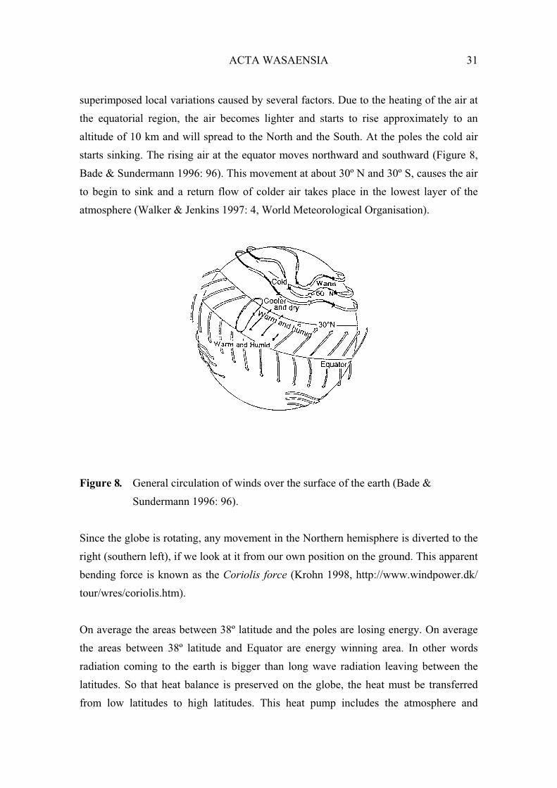
superimposed local variations caused by several factors. Due to the heating of the air at

the equatorial region, the air becomes lighter and starts to rise approximately to an

altitude of 10 km and will spread to the North and the South. At the poles the cold air

starts sinking. The rising air at the equator moves northward and southward (Figure 8,

Bade & Sundermann 1996: 96). This movement at about 30º N and 30º S, causes the air

to begin to sink and a return flow of colder air takes place in the lowest layer of the

atmosphere (Walker & Jenkins 1997: 4, World Meteorological Organisation).

Figure 8. General circulation of winds over the surface of the earth (Bade &

Sundermann 1996: 96).

Since the globe is rotating, any movement in the Northern hemisphere is diverted to the

right (southern left), if we look at it from our own position on the ground. This apparent

bending force is known as the Coriolis force (Krohn 1998, http://www.windpower.dk/

tour/wres/coriolis.htm).

On average the areas between 38º latitude and the poles are losing energy. On average

the areas between 38º latitude and Equator are energy winning area. In other words

radiation coming to the earth is bigger than long wave radiation leaving between the

latitudes. So that heat balance is preserved on the globe, the heat must be transferred

from low latitudes to high latitudes. This heat pump includes the atmosphere and

32 ACTA WASAENSIA

oceans, which transfer about 30 % of the total heat amount (Figure 9, Tammelin 1991b:

17).

Figure 9. Medium radiation degree in the northern half of the globe (Tammelin

1991b: 17).

The flows appearing in the atmosphere can be split into many magnitude events. The

most important factors in the large scale flows are

– uneven warming of the globe

– the rotation of the globe

The relative movement of air in relation to the rotary movement of globe is called

wind. The following forces affect in the atmosphere:

1. Gravitation force

2. Pressure gradient force

3. Friction force

4. Centrifugal force

5. Coriolis force

ACTA WASAENSIA 33

2.3.2 The Height Effect

Figure 10. A principal description concerning the wind speed at different height

levels (Tammelin 1991b: 20).

In the above figure the wind speed at the height uz at different height levels and

geostrophic wind speed vg the ration of vertical change, as well as the so called gradient

height above the different terrain type. h = height of obstacle, d = so called zero level

transition, = describes the exponent of vertical change of speed and Zg = height,

where the terrain no longer has an effect on wind speed

The earth surface resists the movement of air, the force depends on among other things

the speed of movement and the roughness of the earth’s surface (Figure 10, Tammelin

1991b: 20). The friction force weakens the speed of the wind and turns its direction to

lower air pressure.

The changes of wind speed can be described with the standard deviation of the speed,

where

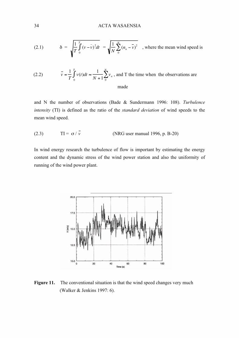
34 ACTA WASAENSIA

(2.1) =1

T(v v

_

)2dt0

T

= 1

N(nn v)2

0

N

, where the mean wind speed is

(2.2) v =1

Tv(t)dt

1

N +10

T

vn0

N

, and T the time when the observations are

made

and N the number of observations (Bade & Sundermann 1996: 108). Turbulence

intensity (TI) is defined as the ratio of the standard deviation of wind speeds to the

mean wind speed.

(2.3) TI = / v (NRG user manual 1996, p. B-20)

In wind energy research the turbulence of flow is important by estimating the energy

content and the dynamic stress of the wind power station and also the uniformity of

running of the wind power plant.

Figure 11. The conventional situation is that the wind speed changes very much

(Walker & Jenkins 1997: 6).

ACTA WASAENSIA 35

In Figure 11 the change is during one second about 2,5 m/s. The measuring period is

100 seconds and measuring height 33 m. (Walker & Jenkins 1997: 6.)

The larger the turbulence intensity is (Tammelin 1991: 28),

– the worse the power calculated from the real speed corresponds to the real

measured total power (energy) during the time period

– the larger is the real dynamic stress directed onto the construct compared to the

calculated stress of the mean wind speed

– the more uneven is the momentary power distribution to the rotor area of the wind

power station.

– the more unevenly the power station rotates

The turbulence is restricted in practice to the lowest layer of the atmosphere, where

height varies with time, stability and weather from 0,1 to 2 km. Typical height is 300–

1000 m.

Figure 12. Representation of wind flow in the boundary layer near the ground

(Walker & Jenkins 1997: 7).

36 ACTA WASAENSIA

The wind speed increases with height most rapidly near the ground, increasing less

rapidly with greater height (Figure 12, Walker & Jenkins 1997: 7). Two of the more

common functions which have been developed to describe the change in mean wind

speed with height are based on experiments:

Power exponent function

(2.4) V(z) = Vr ( )

where z is the height above ground level, Vr is the wind speed at the reference height zr

above ground level, V(z) is the speed at height z, and is an exponent which depends on

the roughness of the terrain.

Logarithmic function

(2.5) V(z) = V(zr)

where V(zr) is the wind speed at height zr above ground level and z0 is the roughness

length (height) (Walker & Jenkins 1997: 7).

The Weibull distribution has received most use in compressing wind data and in energy

assessment analyses and wind load studies (Frost & Aspliden 1998: 386).

Weibull function

(2.6) Rf =k

A(v

A)

k 1

ev

A

k

where Rf is the relative frequency of wind speeds, A the scale factor and k shape the

factor (Figure 13).

ACTA WASAENSIA 37

Rf (%)

0,00 %

2,00 %

4,00 %

6,00 %

8,00 %

10,00 %

12,00 %

1 4 7

10 13 16 19 22 25

Figure 13. Relative frequency distribution special case k=2 Rayleigh distribution.

The measurement of wind speeds is usually carried out using a cup anemometer. The

cup anemometer has a vertical axis and three cups which capture the wind. The number

of revolutions per minute is registered electronically.

Normally, the anemometer is fitted with a wind vane to detect the wind direction. Other

anemometer types include ultrasonic or laser anemometers which detect the phase

shifting of sound or coherent light reflected from the air molecules. The advantage of

non-mechanical anemometers may be that they are less sensitive to icing. In practice,

however, cup anemometers tend to be used everywhere, and special models with

electrically heated shafts and cups may be used in arctic areas.

The best way of measuring wind speeds at a prospective wind turbine site is to fit an

anemometer to the top of a mast which has the same height as the expected hub height

of the wind turbine to be used. This way one avoids the uncertainty involved in

recalculating the wind speeds to a different height.

Guyed, thin cylindrical poles are normally preferred over lattice towers for fitting wind

measurement devices in order to limit the wind shade from the tower.

38 ACTA WASAENSIA

The poles come as kits which are easily assembled, and you can install such a mast for

wind measurements at (future) turbine hub height without a crane. Anemometer, pole

and data logger will usually cost somewhere around 10,000 USD.

The data on both wind speeds and wind directions from the anemometer(s) are collected

on electronic chips on a small computer, a data logger, which may be battery operated

for a long period (Figure 14). Once a month or so you may need to go to the logger to

collect the chips and replace them with blank chips for the next month's data.

If there is much freezing rain in the area, or frost from clouds in mountains, you may

need a heated anemometer, which requires an electrical grid connection to run the

heater. (Krohn 1998, http://www.windpower.dk/tour/wres/windspeed.htm).

Figure 14. NRG Symphonie logger unit.

2.3.3 Energy in the Wind

The kinetic energy in a flow of air through a unit area perpendicular to the wind

direction is E = 1/2mv

2. Through the unit area flowing mass flows m

.

= A dx /dt = A v

in other words the power is

(2.7) P = 1/2 Av

3

where is the air density (kg/m3), v wind speed (m/s) and P is power (watt or joule/s).

ACTA WASAENSIA 39

The air density is the function of air pressure and temperature:

Density ration

(2.8)

where 0 is the dry air density along the International Civil Aviation Organisation

(ICAO) standard temperature and pressure (1.225 kg/m3, 15°C (288.16 K), 1013.25

mbar, Haapanen 1972: 6).

In offshore conditions air humidity can increase. An air steam statistical change is in the

open air between 65 – 90 %. In the same reference in Sweden Lund, Stockholm,

Haparanda and Östersund the air steam partial pressure changes from 2 to 11 mmhg.

Compared to normal pressure 760 mmhg the ratio is 0.3 – 1.4 %. The effect on the

density of air and to power is not notable (Strömberg 1953 p.604).

The temperature change effect is bigger. For example -30 to +30 °C or 243 and 303°K

divided by 288 equals to +18.5 % and -4.9 % for density and power. The air

temperature changes are taken into account in energy calculations.

The air pressure change effect is less than the temperature change. For example 980 –

1060 mbar divided by 1013 equals to –3.2 to +4.6 % for density and power. The air

pressure changes are also taken into account in energy calculations.

The theoretical power P = 1/2 Av

3 is not realised in real wind power plant wings. The

limiting factor is the formula known as the Betz clause (1919), which limits the power

coefficient cp to 59 % of theoretical power. In addition there are other factors, which in

practise limit the power depending on wind speed after the turbine from a maximum

59 % to zero (Gasch & Maurer 1996: 122). The power coefficient cp dependency on

wind speed before v1 and after v3 the turbine is showed in figure 15. The maximum

power coefficient cp, max 0.59 will be reached with the ratio v3/v1 = 1/3.

40 ACTA WASAENSIA

Figure 15. The power coefficient cp dependency on wind speed before v1 and after v3

the turbine (Gasch & Maurer 1996: 122).

In addition there are a lot of other factors which limit the power from the wind mill

manufacturer given the wind speed / power curve. For example one practice curve

follows in the straight part the formula P = 1/2 Av

2,2.

Figure 16. Three keystones connecting with wind power economy (Bade &

Sundermann 1996: 111).

hi distribution of Ws’s

Pi Power in certain Ws

Ei Energy

ACTA WASAENSIA 41

In Figure 16 the first distribution is the wind speed distribution in the measuring place.

It describes each speed percent density. Instead of percentages the hour number of each

speeds can be used. The second distribution describes the power given by the turbine on

each wind speed. The last distribution tells how much wind energy is produced during

the measuring period. The first and second distribution are multiplied and the result is

the energy at the corresponding wind speed (Bade & Sundermann 1996: 111).

The definite energy produced by the wind turbine will be obtained by multiplying the

wind speed distribution values generated from the wind speed measurement with

corresponding power and adding the kilowatt hours together to the total energy. The

other way is to multiply the measured wind speeds with corresponding power and add

them together to the total energy during the examination period.

A rough estimation is that the offshore wind speed level is 15 % higher than onshore

winds. The theoretical power formula P = 1/2 Av

3 promises 50 % more energy. The

reason to go offshore is the better wind speed. It is measured in two places on Kaijakari

(Appendix 4 and Table 17) 1.5 km from land on an island. There the measured energy

was 13.9 % better than onshore on a breakwater. The other case Strömmingsbåda is 19

km out to sea (appendix 5 and table 23). The wind speed difference at a 40 m height is

22.5 % and energy difference 43.8 %. At 60 m height the differences are for wind speed

13.3 % and energy 21.0 %. This can be due to land effect; the forest does not so much

affect the wind speed at 60 m height.

2.4 Wind Energy Economics

The most important question in using wind energy is the economy of wind energy. The

economy determines the success or failure of the whole wind energy area. Wind energy

economy is the sum of many variables.

Today wind energy is competitive (in a narrow economic sense) at specific sites with

favourable conditions, as stated in the Commission's Green Paper "For a European

Union Energy Policy". If external/social costs are included, it is estimated that wind

power in many countries is already competitive with fossil and nuclear power.

42 ACTA WASAENSIA

Several international organisations without preference for wind power estimate that

wind power in a near-term time frame (2005 to 2010) will be competitive with fossil

and nuclear power in a narrow economic sense, without taking into account the

competitive advantage of wind power on external or social costs.

Project preparation costs depend heavily on local circumstances, such as the condition

of the soil, road conditions, proximity to electrical grid sub-stations, etc. As a rule of

thumb project preparation costs on flat on-shore sites can be estimated to be 33 % of ex

works turbine costs. (Krohn 1998, http://www.windpower.dk /tour/econ/index.htm).

Operation and maintenance costs include service, consumables, repair, insurance,

administration, lease of site, etc. The annual operation and maintenance cost is often

estimated as 3 % of ex works cost of a wind turbine (or 1 c /kWh, which is the same

with 3000 operational hours and with 1 MW costs 1 M ).

Technical life time or design life time for European machines is typically 20 years.

Individual components should be replaced or renewed at a shorter interval.

Consumables such as oil in the gearbox, braking clutches, etc. are often replaced at

intervals of 1 to 3 years. Parts of the yaw system are replaced at intervals of 5 years.

Vital components exposed to fatigue loads such as main bearings, bearings in the

gearbox and generator are foreseen to be replaced halfway through the total design life

time.

Figure 17 shows OECD´s collected nuclear, coal and gas prices in different countries

and wind power prices from the same period (Source: OECD 1993). For comparison:

average new wind power in Germany 5.6 US cent/kWh, Denmark 4.1 US cent/kWh (at

1991 price level)

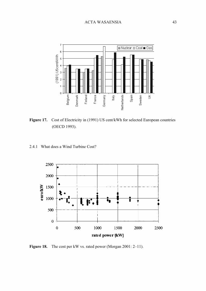
ACTA WASAENSIA 43

Figure 17. Cost of Electricity in (1991) US cent/kWh for selected European countries

(OECD 1993).

2.4.1 What does a Wind Turbine Cost?

Figure 18. The cost per kW vs. rated power (Morgan 2001: 2–11).

44 ACTA WASAENSIA

The graph above gives an impression of the price range of modern, grid connected wind

turbines (Figure 18, Morgan 2001: 2–11). The prices vary for each generator size,

different tower heights and rotor diameters. One extra metre of tower will cost roughly

1 500 USD. A special low wind machine with a relatively large rotor diameter will be

more expensive than a high wind machine with a small rotor diameter (Krohn 1998,

http://www.windpower.dk /tour/econ/index.htm).

Commercial offshore wind turbines are made by 10 manufacturers, in rotor diameter the

size range is 65 to 80 metres and rated power 1.5–2.5 MW. Hub height follows the

length of rotor diameter. New offshore turbines are under design with rotor diameter of

120 m and power 5–6 MW (Morgan et al 2001: 2–6). According Barthelmie et al.

(2001: 6–2 and 6–3) onshore wind investments are M 1 / MW and the costs for

offshore wind power are M 1.5 / MW. Table 3 shows one cost distribution of on- and

offshore cases. The distribution varies case by case.

Table 3. Investment cost by component, one example (Barthelmie et al. (2001:6–3).

Onshore (%) Offshore (%)

Foundations 5. 5 16

Turbines 71 51

Internal electrical grid 6. 5 5

Electrical system 0 2

Grid connection 7. 5 18

O&M facilities 0 2

Engineering and admin. 2. 5 4

Miscellaneous 7 2

Total 100 100

2.4.2 Installation Costs for Wind Turbines

Installation costs include 1. foundations, normally made of armed concrete, 2. road

construction (necessary to move the turbine and the sections of the tower to the building

site), 3. transformer (necessary to convert the low voltage (690 V) current from the

ACTA WASAENSIA 45

turbine to 20 kV current for the local electrical grid, 4. telephone connection for remote

control and surveillance of the turbine, and 5. cabling costs, i.e. the cable from the

turbine to the local 20 kV power line.

The installation costs vary. The costs of roads and foundations depend on soil

conditions, i.e. how cheap and easy it is to build a road capable of carrying 30 tonne

trucks. Another variable factor is the distance to the nearest ordinary road, the cost of

getting a mobile crane to the site, and the distance to a power line capable of handling

the maximum energy output from the turbine. A telephone connection and remote

control is not a necessity, but is often fairly cheap, and thus economic to include in a

turbine installation. Transportation costs for the turbine may enter the calculation if the

site is very remote, though usually they will not exceed 15 000 USD.

It is obviously cheaper to connect many turbines in the same location, rather than just

one. On the other hand, there are limits to the amount of electrical energy the local

electrical grid can handle. If the local grid is too weak to handle the output from the

turbine, there may be need for grid reinforcement, i.e. extending the high voltage

electrical grid. It varies from country to country who pays for grid reinforcement – the

power company or the owner of the turbine (Krohn 1998, http://www.windpower.dk

/tour/econ/install.htm).

2.4.3 Operation and Maintenance Costs for Wind Turbines

Modern wind turbines are designed to work for 120 000 hours of operation throughout

their design lifetime of 20 years. That is far more than an automobile engine which will

generally last for some 4 000 to 6 000 hours.

Experience shows that maintenance cost are generally very low while the turbines are

brand new, but they increase somewhat as the turbine ages.

46 ACTA WASAENSIA

Most of the maintenance cost is the regular service of the turbines, but some people

prefer to use a fixed amount per kWh of output in their calculations, usually around 0.01

USD. The reasoning behind this method is that wear and tear on the turbine generally

increases with increasing production.

Other than the economies of scale which vary with the size of the turbine, as mentioned

above, there may be economies of scale in the operation of wind parks rather than

individual turbines. These economies are related to the semi-annual maintenance visits,

surveillance and administration, etc.

The turbine lifetime extension means that some wind turbine components are more

subject to tear and wear than others. This is particularly true for rotor blades and

gearboxes. Wind turbine owners who see that their turbine is close the end of their

technical design lifetime may find it advantageous to increase the lifetime of the turbine

by doing a major overhaul of the turbine, e.g. by replacing the rotor blades.

The price of a new set of rotor blades, a gearbox, or a generator is usually in the order of

magnitude of 15–20 per cent of the price of the turbine.

The 20 year design lifetime is a useful economic compromise which is used to guide

engineers who develop components for the turbines. Their calculations have to prove

that their components have a very small probability of failure before 20 years have

elapsed.

The actual lifetime of a wind turbine depends both on the quality of the turbine and the

local climatic conditions, e.g. the amount of turbulence at the site, as explained in the

page on turbine design and fatigue loads.

Offshore turbines may e.g. last longer, due to low turbulence at sea. This may in turn

lower the costs, see page 42 (Krohn 1998, http://www.windpower.dk /tour/econ/oandm.

htm).

ACTA WASAENSIA 47

2.4.4 Income from Wind Turbines

Figure 19. Energy Output from a Wind Turbine (Krohn 1998).

Figure 19. represents a typical Danish 600 kW turbine production at the separate wind

speeds. The graph shows how annual energy production in gigawatt hours varies with

the windiness of the site depending on the three different k-values (see shape factor,

Weibull function, Chapter 5.2). With a mean wind speed of, approximately 6.75 metres

per second at hub height, you get about 1.5 million kilowatt hours of energy per year.

The figures for annual energy output assume that wind turbines are operational and

ready to run all the time. In practice, however, wind turbines need servicing and inspec-

tion once every six months to ensure that they remain safe. In addition, component

failures and accidents (such as lightning strikes) may disable wind turbines.

Very extensive statistics show that the best turbine manufacturers consistently achieve

availability factors above 98 per cent, i.e. the machines are ready to run more than 98

per cent of the time. Total energy output is generally affected less than 2 per cent, since

wind turbines are never serviced during higher winds.

Such a high degree of reliability is remarkable, compared to other types of machinery,

including other electricity generating technologies. The availability factor is therefore

usually ignored when doing economic calculations, since other uncertainties (e.g. wind

variability) are far larger.

48 ACTA WASAENSIA

Not all wind turbine manufacturers around the world have a good, long reliability

record, however, so it is always a good idea to check the manufacturers’ track record

and servicing ability before you go out and buy a new wind turbine (Krohn 1998, http:

//www.windpower.dk /tour/econ/income.htm).

2.4.5 Wind Energy and Electrical Tariffs

Electricity companies are generally more interested in buying electricity during the

periods of peak load (maximum consumption) on the electrical grid, because this way

they may save using the electricity from less efficient generating units. According to a

study on the social costs and benefits of wind energy by the Danish AKF institute, wind

electricity would be some 30 to 40 per cent more valuable to the grid, if it were

produced completely randomly (Krohn 1998, http://www.windpower.dk /tour/

econ/tariffs.htm).

In some areas, power companies apply variable electricity tariffs depending on the time

of day when they buy electrical energy from private wind turbine owners. Normally,

wind turbine owners receive less than the normal consumer price of electricity, since

that price usually includes payment for the power company’s operation and mainte-

nance of the electrical grid, plus its profits.

Many governments and power companies around the world wish to promote the use of

renewable energy sources. Therefore they offer a certain environmental premium on

wind energy, e.g. in the form of a refund of electricity taxes etc. on top of normal rates

paid for electricity delivered to the grid.

Large electricity consumers are usually charged both for the amount of energy (kWh)

they use, and for the maximum amount of power (kW) they draw from the grid. The

reason they have to pay more is that it obliges the power company to have a higher total

generating capacity (more power plant) available. Power companies have to consider

adding generating capacity whenever they give new consumers access to the grid. But

with a modest number of wind turbines in the grid, wind turbines are almost like

"negative consumers". They postpone the need to install other new generating capacity.

ACTA WASAENSIA 49

Many power companies therefore pay a certain amount per year to the wind turbine

owner as a capacity credit. The exact level of the capacity credit varies. In some

countries it is paid on the basis of a number of measurements of power output during

the year. In other areas, some other formula is used.

Most wind turbines are equipped with asynchronous generators, also called induction

generators. These generators require current from the electrical grid to create a magnetic

field inside the generator in order to work. As a result the alternating current in the

electrical grid near the turbine will be affected (phase-shifted). This may at certain times

decrease (though in some cases increase) the efficiency of electricity transmission in the

nearby grid, due to reactive power consumption. In most places around the world, the

power companies require that wind turbines be equipped with electric capacitors which

partly compensate for this phenomenon. (For technical reasons they do not want full

compensation). If the turbine does not live up to the power company specifications, the

owner may have to pay extra charges. Normally, this is not a problem which concerns

wind turbine owners, since experienced manufacturers routinely will deliver according

to local power company specifications (Krohn 1998, http://www.windpower.dk /tour/

econ/tariffs.htm).

2.4.6 Basic Economies of Investment

What society gets in return for investment in wind energy is pollution-free electricity.

The private investor in wind energy can make investments which have a high rate of

return before tax and will have an even higher rate of return after taxes. The reason for

this is the depreciation regulations. With rapid tax depreciation it is possible to get a

higher return on an investment, because it is allowed to deduct the loss of value of your

asset faster than it actually loses its value.

The difference between the value of today’s and tomorrow’s dollars is the interest rate.

One dollar a year from now is worth 1 / (1+r) today. r is the interest rate, for example 5

per cent per year.

50 ACTA WASAENSIA

By taking inflation into account dollars have the same purchasing power as dollars do

today. Economists call this working with real values, instead of nominal ones.

An investment in a wind turbine gives a real return, i.e. electricity, and not just a

financial (cash) return. This is important, because if general inflation of prices during

the next 20 years is expected, then it will also be expected that the electricity prices will

follow the same trend.

Likewise, it is expected that operation and maintenance costs will follow roughly the

same price trend as electricity. If all prices move in parallel (with the same growth rates)

over the next 20 years, then the calculations are using real values which represent a

fixed amount of purchasing power.

To calculate the real rate of return (profitability) of wind energy, the real rate of interest

is usual, i.e. the interest rate minus the expected rate of inflation (1+r) / (1+i). For

example, the annuity factor for an interest rate of 5 % and 20 years is 8.024 %.

Years\% 2 3 4 5 6 7 8

10 0.111 0.117 0.123 0.130 0.136 0.142 0.14915 0.078 0.084 0.090 0.096 0.103 0.110 0.117

20 0.061 0.067 0.074 0.080 0.087 0.094 0.102

25 0.051 0.057 0.064 0.071 0.078 0.086 0.09430 0.045 0.051 0.058 0.065 0.073 0.081 0.089

Typical real rates of interest for calculation purposes these days are in the vicinity of 5

per cent per annum or so. In countries like Western Europe they could be even down to

3 per cent. By using the bank rate of interest the nominal calculations will be made, i.e.

add price changes everywhere, including the price of electricity (Krohn 1998,

http://www.windpower.dk /tour/econ/basic.htm).

ACTA WASAENSIA 51

2.4.7 Wind Energy Economics

Figure 20. The cost of electricity varies with annual production (Krohn 1998).

In Figure 20 the cost of electricity produced by a typical Danish 600 kW wind turbine

varies with annual production (i 5%, r 20 years and the investment 0.6875 MUSD). To

produce twice as much energy per year, the price is half the cost per kilowatt hour.

There is no such thing as a single price for wind energy. Annual electricity production

will vary enormously depending on the amount of wind at the turbine site. Therefore

there is no single price for wind energy, but a range of prices, depending on wind

speeds.

The graph below shows the relationship between wind speeds and costs per kWh. This

is based on examples. The wind speeds at 50 metre hub height will be some 28 to 35 per

cent higher (for roughness classes between 1 and 2) than at a height of 10 metres, which

is usually used for meteorological observations.

52 ACTA WASAENSIA

Figure 21. Cost of electricity, example 600 kW turbine (Krohn 1998).

The example in Figure 21 is for a 600 kW wind turbine with a project lifetime of 20

years; investment = 585 000 USD including installation; operation & maintenance cost

= 6750 USD/year-, 5% p.a. real rate of interest-, annual turbine energy output taken

from power density calculator using a Rayleigh wind distribution (shape factor = 2)

(Krohn 1998, http://www.windpower.dk /tour/econ/economic.htm).

2.4.8 Economics of Offshore Wind Energy

In 1997 the Danish electrical power companies and the Danish Energy agency finalised

plans for large scale investment in offshore wind energy in Danish waters.

The plans imply that some 4 400 MW of wind power are to be installed offshore before

the year 2030. Wind power would by then provide some 40 to 50 per cent of Danish

electricity consumption (out of a total of 35 TWh/year 1999).

The most important reason why offshore wind energy is becoming economic is that the

cost of foundations has decreased dramatically. The estimated total investment required

to install 1 MW of wind power offshore in Denmark is around 2 million today. This

includes grid connection, etc.

ACTA WASAENSIA 53

Since there is substantially more wind at sea than on land, however, we arrive at an

average cost of electricity of some 0.36 DKK/kWh = 0.05 USD/kWh = 0.09 DEM/kWh.

(5% real discount rate, 20 year project lifetime, 0.08 DKK/kWh = 0.01 USD/kWh =

0.02 DEM in operation and maintenance cost).

Figure 22. A project lifetime’s effect on the costs (Krohn 1998).

It would appear that turbines at sea would have a longer technical lifetime, due to lower

turbulence. The cost sensitivity to project lifetime is plotted in Figure 22. If a project

lifetime is 25 years instead of 20, this makes costs 9 per cent lower, at some 0.325

DKK/kWh.

Danish power companies, however, seem to be optimising the projects with a view to a

project lifetime of 50 years. This can be seen from the fact that they plan to require 50

year design lifetime for both foundations, towers, nacelle shells, and main shafts in the

turbines. (Krohn 1998, http://www. windpower.dk /tour/econ/offshore.htm)

If assumed that the turbines have a lifetime of 50 years, and add an overhaul

(refurbishment) after 25 years, costing some 25 per cent of the initial investment (this

figure is purely a numerical example), we get a cost of electricity of 0.283 DKK/kWh,

which is similar to average onshore locations in Denmark. (Krohn 1998, http://www.

windpower.dk /tour/econ/offshore.htm)

54 ACTA WASAENSIA

2.4.9 Employment in the Wind Industry

The wind industry in 1995 employed some 30,000 people world wide. It includes both

direct and indirect employment. By indirect employment we mean the people who are

employed in manufacturing components for wind turbines, and the people who are

involved in installing wind turbines world wide.

In 2000 the Danish wind industry employed 16 000 people. Wind turbine production

creates about 50 per cent more jobs, since Danish manufacturers import many compo-

nents, e.g. gearboxes, generators, hubs, etc. from abroad. In addition, jobs are created

through the installation of wind turbines in other countries (Krohn 1998, http://www.

windpower.dk /tour/econ/empl.htm).

B.Smith et al. (2001: 8–1) calculates a figure of 4.52 full time direct jobs per MW by

industry sector as a result of installing some 10 000 MW of offshore wind power, see

Table 4. These are direct workers. Calculating from the offshore wind power investment

price of 1.5 M / MW and taking as the cost for one worker around 0.04 M /year

(Statistical Yearbook, 1999) the need being 4.52 workers/MW, then one worker should

make one MW in 8.3 years (1.5M /MW / 4.52FTJ/MW / 0.04M /y = 8.3 year/FTJ). A

rough calculation with the same figures, 1.5M /MW / 0.04M /working year makes 37.5

working years/MW or 37.5 people/MW/year but including all white, blue collar and all

subcontracting people. It is assumed that nearly the whole turbine costs in the chain

from first subcontractor to assembly work are working costs (author).

ACTA WASAENSIA 55

Table 4. Estimate of direct employment to develop offshore wind farms (B.Smith et

al. (2001: 8–1).

Full Time

Jobs/MW

Project design and

Development

Marine/Ground investigations

Site development including permissions

Design including structural, electrical

And resource

Finance

0.01

0.1

0.02

0.04

Component supply Generator

Gearboxes

Rotor blades

Brakes, hydraulics

Electrical & control system

Towers

0.15

0.9-0.4

0.5

0.04

0.04

0.9

Assembly Wind turbines 1

Installation Foundation structure

Electrical and connecting cables

Wind turbines

Project management & commissioning

0.3

0.05

0.3

0.11

Operation &

Maintenance

Management, routine and fault

Maintenance

0.06

TOTAL 4.52

2.5 Offshore Wind Power

Wind power’s extensive potential is on the sea. Even a short movement from the coast-

line to the sea improves the wind conditions remarkably. In addition there is less

regulation in building at sea than building on shore. The building at sea compared to on

land, however, creates many additional costs. The cabling lengthens and more

demanding foundations on a sea location raises foundation costs. The additional costs

can be even larger in a location where waves or ice cause stress to the foundation and

structure of a power station.

56 ACTA WASAENSIA

The size of wind power stations has grown during the last 10 years to the megawatt

class. In 1997 the most common size was 600 kW, but 2.5 MW power stations have

been on the market in 2000. Bigger power stations are especially tempting when

building at sea, since the foundation costs do not rise compared to the reached

production advantage.

2.5.1 Offshore Wind Power in Europe

In Finland in 1994 the offshore wind power building potential on small islands was

researched. Then the potential on scars and islands was estimated to be 30 TWh/a, of

which about 4 TWh/a could be built without strengthening the electricity net on the

coast. The building on small islands reduces the foundation costs significantly

compared to building on the sea bottom. However it improves substantially the

production compared to building on shore. Nature reserve areas and holiday settlements

severely restrict the use of small islands for wind power production (Sommardal et al

1994).

By the end of the year 2000 offshore wind power stations and parks have been built in

Denmark, Holland, Sweden and the UK about 80 MW. In addition, the previous

countries and Ireland, Germany, Belgium and some other counties have a target

installation of 10 950 MW by 2030. In Appendix 14 are plans for 38 parks. The mapped

offshore resource estimate in 14 European countries is in total 138 600 MW (Barthelmie

et al. 2001: 4–2).

2.5.2 Experience from Realised Offshore Wind Power Projects

World wide nine offshore wind projects have been realised: in Denmark, in Holland, in

Sweden and in UK. All projects are rather close to the coast and the water depth is in

the site 3–8 m. Table 5 shows offshore projects: capacity (MW), distance from coast

(km), total investment (M ) and average year’s production (Holttinen et al 1998: 15,

modified by BTM Consult ApS – March 2001).

ACTA WASAENSIA 57

Table 5. Realised offshore wind power projects.

Country Site Units Size/Producer MW Year Km Invest

M

Production

MWh/a

Denmark Vindeby 11 450kW/Bonus 4.95 1991 1.5 10.4 11 700

Holland Lely 4 500 kW/Nedwind 2.0 1994 1 4.54 4 000

Denmark Tunö Knob 10 500 kW/Vestas 5.0 1995 6 10.4 15 000

Holland Dronten 19 600 kW/Nordtank 11.4 1996 0.3 19.0

Sweden Bockstigen 5 550kW/WindWorld 2.75 1997 4 4.0 8 000

Sweden Utgrunden 7 10.5 MW/Tacke 10.5 2000 12 38 000

Denmark Middelgrunden 20 2 MW/Bonus 40 2000 48.8 90 000

UK Blyth 2 2 MW/Vestas 3.8 2000 1

Total by end 2000 78 80.4

At sea the wind is clearly smoother than on land, since there are no obstacles. Less

turbulence means that the fatigue load is smaller. It is probable that the life time for a

wind power plant is longer than on land. Offshore wind power plants can be used

probably for 25 years instead of 20 years. In addition, the foundations can be planned

for 50 years of operating life. Then it is possible to exploit the foundations for two wind

power plants.

In Denmark it has been noticed in offshore wind power plant building that if the

location is further from the coast the production estimates will be exceeded by even 30

% . Earlier it was supposed that by building at sea the power plant’s distance between

turbines should be increased, because the more laminar flow at sea would create more

disturbances in the flow field far on rotor’s background than in onshore conditions. The

experiences on the Tunö Knob offshore wind park have, however, indicated that the

shadow effect between the turbines is smaller than estimated.

By placing the offshore wind power plants several kilometres from the coast it is

possible to accelerate the rotor rotation speed. This increases running noise, but at the

same time it increases production. In the case of Tunö Knob the rotation speed was

increased from 30 to 33 revolutions per minute. On the basis of experience it is possible

to increase the rotation speed still more.

58 ACTA WASAENSIA

Experience of offshore wind power plants shows that accessibility should still be

developed further: for example it is not possible to get to the Tunö Knob power plant if

the wave height is over one meter.

The offshore wind power plant costs are clearly higher than the costs of land built

power plants. For example the Windeby production costs are about 8.75 c/kWh and

Tunö Knob 7.23 c/kWh (without the demonstration phase costs 6.39 c/kWh). In the

last project in Sweden the calculated costs are nearer to 5.05 c/kWh. The costs will in

addition decrease further when the new megawatt class plants come on to the market

and the foundation technology is developed (Holttinen et al. 1998: 16).

2.5.3 Building of large Wind Power Parks

100–200 MW size wind power park projects have been planned in Denmark, Germany,

Sweden, Holland and Spain. Estimated production costs are 5.05–6.73 c/kWh (In land

built projects the production costs are 3.36–4.20 c/kWh.

In Denmark a strong movement towards the building of wind power stations arises

partly from the need for coal oxide reduction. In 1997 a plan was published for building

4000 MW offshore by the year 2030. The plan was published by a committee with

representatives of the biggest power company (ELSAM and ELKRAFT) and a Danish

cabinet member. Areas for wind power production were not allowed for other users

(fishing, defence forces, nature protection areas, etc.) and they had to be 4–10 m in

depth and 15–30 km from the land. About 1000 km2 of suitable areas was found (8000

MW).

It is the intention in Denmark to build 120–150 MW parks which will be placed as far

from the coast as is technically and economically reasonable, in other words about 15–

30 km from land. The first stage of the plan identifies six areas on which will be built

together over 700 MW of wind power during 2000–2006. The investment costs are

expected to drop by about 25 % from the level of the first Danish offshore park, in other

words to be 10–12 million DKK/MW. The production costs are estimated at about

4.71–5.05 c/kWh (Holttinen et al. 1998: 18).

ACTA WASAENSIA 59

Figure 23. The existing and proposed offshore wind farms in the North Sea and Baltic

Sea (New Energy 2/2000).

Figure 23 shows the existing and planned wind farms in Sweden, Denmark, Germany,

Netherlands and UK (New Energy 2/2000, p. 28 and 3/2000, p. 28 more offshore plans

in Appendix 14).

In Holland there is a long term plan to achieve 3000 MW wind power by the year 2020.

Half of this is planned to be built at sea. In Holland a similar mapping to that made in

Denmark was been carried out concerning potential offshore wind park areas near the

coast. At this moment the first big offshore wind park 100 MW is being constructed

60 ACTA WASAENSIA

about 8 km from the coast. According to the plan the building will be completed at the

earliest in 2001. The production costs of the first large wind park exceed 6.73 c/kWh.

For the production costs to be appropriate for a site this far from the coast, the size of

the park should be 100–200 MW. The large size of the park and the lack of experience

in construction are an economic risk, so that it is appropriate to first place a smaller park

nearer to the coast even if the production costs are larger (Holttinen et al 1998: 18).

2.6 Offshore Foundation Technique

In freezing sea areas the constructs are open to a harsh environment of stresses such as

corrosion, erosion and ice – and wave loads. By formatting the foundations the ice load

can be reduced remarkably. The design should take into consideration both local high

ice pressures and cumulated total ice loads from large area, both static and dynamic

loads.

2.6.1 Offshore Constructs in Ice Conditions

A traditional water foundation construct is the caisson. Its mass holds the construct both

upright and prevents the caisson gliding horizontally, Figure 24a. A continuation

development is the so-called hems caisson where the hems penetrate to the bottom and

increase glide resistance, Figure 24i. Another way is to ram piles through the caisson for

increasing glide resistance, Figure 24j. With piles it is possible to increase at the same

time the bearing capacity of the foundation against bending moment. The caisson is

characteristically a massively stiff construct. Its dimensions depend on prevailing loads

and on the bearing capacity of the sea bottom. The caisson foundation will be fabricated

in a dry dock, floated to the site, embedded and loaded. Finally erosion protection will

be carried out. The caisson foundation can be made in rather shallow water. The floating

stability of the caisson also allows upper construct (wind turbine tower) assembly on the

caisson in the dock.

ACTA WASAENSIA 61

Another traditional foundation method is a pile rammed into the sea bottom, Figure 24c,

or a pile anchored into a rock gully, Figure 24e. The gully is possible to compensate

also with anchor bolts into the rock, Figure 24f. The dimension and foundation depth

depends on the load and density of the bottom, friction and cohesion. The pile is lighter

than the caisson and flexible, being sensitive to dynamic loads. The primary pile will be

fabricated in the workshop. It can be floated to the site, erected and rammed into the sea

bottom or tagged with concrete into rock with light crane equipment. The upper

construct will be assembled after foundation. Erosion is generally not harmful to pile

foundations.

Constructional effective, although more complicated to realise, are tripod – and grid

foundations, Figures 24g and 24h. They can be anchored into bottom rock or through

ram piles, which is common in oil drilling jacket platforms. Three feet is rather stiff

therefore it also suits ice conditions. With grid – or jacket foundation there can be

accumulation of ice between the feet. Dynamic loads can be harmful. Ready assembled

tripod – or grid construct mounting requires heavy equipment. A jacket type construct

assembly succeeds with lighter equipment. Ramming or anchoring of the pile also

requires jacket piece fixing with concrete injection. The upper construct will be

assembled after foundation.

The form of foundation at the water level determines how the ice will be broken.

Against a vertical structure crushing happens and against an inclined structure bending,

fraction or cutting. With a narrow vertical structure the ice forces can be decreased and

the ice accumulation reduced. But the increased elasticity promotes vibration caused by

ice. The inclined or cone form causes breakage at significantly lower loads than with

crushing against a vertical structure, despite greater breadth of the inclined structure.

However the dynamic ice load effects are on an inclined structure clearly more minor

compared to a vertical structure.

62 ACTA WASAENSIA

ACTA WASAENSIA 63

Figure 24. Different foundation alternatives (Määttänen 1998: 74–77).

The conical form can be realised by a caisson, Figure 24b, with cone collar in the pile

foundation, Figure 24d, or with a cone caisson with thin additional piles, Figure 24j.

The most advantageous form against both static and dynamic ice force at the water level

is the cone but during assembly the stability of the cone at the floating – and sinking

phase of the caisson is bad. The cone collar should be assembled separately after the

basic pile or together with the upper part. By filling the cone with concrete the fastening

of the basic pile and good resistance against local ice pressure will be achieved at the

same time.

g) Tripod + cone h) Grid

i) Caisson + hems

j) Cone caisson + piles

64 ACTA WASAENSIA

The construct form is easier to realise by a vertical construct form at the water level than

with an inclined construct form. A vessel is considerably more difficult to fasten to an

inclined structure because the waves affect the vertical movement of the vessel. During

winter time ice accumulates on the front of a conical structure. This can be a problem

for roads of the foundation (Määttänen 1998: 74–77).

2.6.2 Wind Power Plant Foundation on the Sea

Until now three separate types of foundations have been used on offshore wind power

stations:

1) Gravity foundation which keeps upright through its own weight and with added

weight mass added to the plate

2) Mono pile which is rammed deep into the bottom and stays upright due to the

pressure of the sea bed

3) Tripod where the feet are mounted to the bottom and support the tower which is

mounted on the topside of the feet (Määttänen 1998: 74–77).

The caisson suits several types of sea bottom. The caisson surface pressure is low. It

needs only a smooth base. The cone caisson is suitable in shallow water against ice

pressure. The mono pile needs the right bottom conditions: enough loose soil to allow

ramming and enough stiffness to keep the mono pile upright. Rock well requires a rock

sea bottom. Negative factors are the price and rocky sea bottom exiguity. Tripod and

grid are suitable if it is possible to bolt them into the sea bottom. Several variations

appear but those three main types of foundations (caisson based on gravity, mono pile

based on digging into the sea bottom and tripod legs fastening into the sea bottom) are

always the bases of several foundation variations. These types are universally suited for

sea bottom building, regardless of what the construction is on top of the foundation. For

example, oil rigs follow the same scheme.

The caisson and mono pile type are present in today’s wind turbine offshore parks. The

caisson type needs to dig depression, balance it and gravel it into a horizontal position

less then half a degree from the horizontal. In the erection procedure the use of offshore

cranes and assisting vessels with crews also create costs. The mono pile needs a

ramming operation and the same offshore crane and assisting vessels. Both possibilities

are very near each other. One example, the Middelgrunden 40 MW wind farm

ACTA WASAENSIA 65

associated research (www.middelgrunden.dk/MG_UK/project_info/prestudy.htm) p. 9,

10/14 in Table 6 gives the following prices for the alternatives based on tenders and

realised results:

Table 6. Middelgrunden foundation alternatives.

Caisson type Mono pile

Concrete Steel Steel

0.315 m 0.38 m 0.42 m

0.393 m Realised including changes

2.6.3 Caissons in the Tunö Knob Wind Park, Denmark

Tunö Knob wind park was constructed in 1995. It includes ten 500 kW plants about

6 km from the Jutland coast and about 3 km from Tunö island. The water depth is 3.1–

4.7 m.

Figure 25. Tunö Knob offshore wind power plant (Holttinen et al. 1998).

66 ACTA WASAENSIA

Steel concrete caissons are the foundation type of these plants. They are designed to

resist waves, sea flows, wind loads, ice loads and the loads effected by the wind turbine

itself. The weight of one foundation is about 1000 tons including about 500 tons of

filling sand. The height of the lower part of the cylindrical foundation varies with the

water depth. The upper part is 2.5 m above sea level. The foundation includes the steel

platform and four wooden fender piles. To reduce ice load focusing on the foundation

the platforms and fender piles are designed to break at a certain ice load.

The foundations were built in Århus harbour from January to June 1995. In July these

were transported to the site by a crane barge. They were assembled on the sea bottom on

crushed stone and the caissons were filled with sand. Finally stone erosion protection

was assembled round the foundations.

The wind power plants were erected at the beginning of August 1995 from a crane

barge. The erection of ten wind power stations took only five days. The sea cable

assembly and the finishing of the power stations assembly was completed in September

1995.

The erecting of big sea wind parks should be planned so that the assembly work at sea is

completed in as short a time as possible. Otherwise for example a 100 MW wind power

plant would not be assembled during one summer far from land. In the feasibility study

the concrete caisson was thought to be too heavy. Steel caissons can be placed in several

pieces into the same barge, thus saving time on the erecting work (Holttinen et al 1998:

78–79).

2.6.4 Mono Piles

A wind power plant can also be erected on a 3–4 m diameter steel pile. The pile will be

rammed 15–30 m deep into the sea bottom depending on the water depth and the soil.

The rammed pile is from a production – and erection technology point of view an easier

solution than the caisson, since it uses direct traditional technology and is not as

sensitive to wash erosion (Figure 26). Erosion protection with small stones can,

however, be in place. The problem with rammed pile is the design and measuring of

power station and foundation especially with dynamic vibration. Every power station

ACTA WASAENSIA 67

would need calculations based on sea bottom ground analysis. In Holland a 100 x 1

MW sea wind park building with rammed pile foundations is being planned.

Figure 26. Wind power plant erection with rammed pile foundation (Holttinen et al.

1998).

In Bockstigen in Sweden in 1997 the sea wind park foundation was piles which were

not rammed into the sea bottom but assembled into rock drilled deep holes (Figure 27).

The park includes five 500 kW plants which are located about 4 km from the South

Gotland coast at a location where the water depth is about 6 m. 8–10 m deep holes were

drilled into the sea bottom into the hard rock for the piles. After this 2.25 m diameter

piles were assembled and placed concrete into position. Since the ground on the sea bed

is hard rock, it is expected that the pile side motions will be non-existent.

68 ACTA WASAENSIA

Figure 27. Offshore wind power plant on the Bockstigen wind park (Holttinen et al.

1998).

The wind power turbines were brought onto the site by barge and assembled onto the

piles with the same crane vessel with which the piles were assembled. The used vessel

resembles an oil drilling platform in the sense that it stays on the sea bottom high above

sea level. It was noticed in the project that the used vessel limits the possible erection

time when a transfer of the vessel can happen only on a totally calm sea. The trans-

portation of wind power plant parts turns out to be more complex than was planned

(Holttinen et al 1998: 80–82).

Ice cones are planned for all the basic types which come into direct with it. With the

help of these cones the force of the ice decreases remarkably. The variation of sea level

will be taken into consideration in the design. On the Finnish Gulf of Bothnia the upper

ACTA WASAENSIA 69

surface of the ice cone will extend about 0.5 m above the highest sea level and the

lowest surface under the lowest part of the ice.

The ice cone bends and breaks ice better when the angle between ice and cone is gently

sloping. The friction between ice and the cone increases the effective cone angle, so by

decreasing friction a sharper cone can be built and vice versa. The suitable cone angle

for concrete is about 45–60° and for steel 55–60°. In picture 24d the cone middle

diameter is at the water level. A bigger cone is needed if there is a landing plane above

the cone. The minor values correspond to a tower diameter of 4 m. The friction value

= 0.05 corresponds to the painted steel surface and = 0.3 concrete surface. In cases

when the ice thickness is under 40 cm the ice loads in other cases stay under the 1 MN

level.

The cone can be based on a middle cylinder of foundation and it can be made of either

steel or concrete. A thin steel mantle cast full of concrete inside is a simple and

advantageous solution. The steel mantle decreases friction and acts as casting mould.

When ice blows come from a direction other than the coast a one-sided cone at 180° can

be sufficient and from the direction of the coast this can be in the form of a dam

(Haapanen 1998: 85–86).

2.6.5 Construction Technology

The foundations and wind power station transportation to the site are problems for

which it is not easy to find a cheap solution. The transportable and lifted mass are large.

A foundation weighs hundreds of tons as ready-made concrete and thousands of tons

filled with mass. The weight of a power station, depending on size, is 80–200 tons. The

tower height is 50–80 m.

If the planned site of wind power turbine is shallow water only 1–2 m in depth, heavy

lift equipment is transported to the site by barge either to dredge a channel or build a

causeway for the land transport equipment. On the Finnish Gulf of Bothnia also erection

on the ice can be considered. The power station can be transported over and 3 metres

70 ACTA WASAENSIA

depth of water erected with a crane barge. Also a floated foundation can be used to

which a tower, machinery and a rotor are assembled before floatation.

With the erection of a wind power turbine the effect of waves is taken into consideration

as well as the assembly duration, used equipment and floating stability of the whole

construct. On the basis of local wave statistics it can be estimated at what time of year

assemblies are possible and how long suitable weather windows exist for assembly.

So far offshore wind power plants have been erected at sea either with offshore

equipment (floating crane) or with a crane based on a barge. The erection of megawatt

class plant needs about a 55 ton lifting capacity, nearly 80 m crook height and over 10

m lifting distance from the edge of foundation. There are cranes big enough in Finland

which can be moved onto a barge during erection. This kind of arrangement also needs

an anchoring system and is noticeably sensitive to wind and waves. It suits shallow

water and a sheltered site. A ready floating crane is in this respect a more reliable

solution but considerably more expensive. It is possible for a tower erected at sea to be

60 rather than 70 m in height if the cost of a crane with greater lifting height is

unreasonably high.

When a large offshore wind park is to be constructed, it is attempted to erect it usually

during summer time (under 150 days), so a foundation and power plant erection should

not take many days.

By building 600 kW plants on shore it is possible to erect two plants in one day. A

megawatt class plant construct uses ready-made foundations and in best cases takes one

day. If a strong enough crane is in use, the construct could be accelerated so that the

wind power plant would be lifted in long pieces (for example the tower in one piece, the

machine room in one and the rotor in one piece).

ACTA WASAENSIA 71

The wind power plant can not be erected in strong wind: generally the wind speed

should be under 8 m/s. At sea the weather conditions are especially important, the used

equipment may require even lower wind speeds and wave heights. The best erection

weather is naturally in summer (Haapanen 1998: 96–97).

2.6.6 Costs of Offshore Wind Power Plant

The offshore wind power costs can be divided into 4 main fields: 1) seabed conditions

2) marine environment 3) meteorological conditions and 4) turbine type. The seabed

conditions describe the soil conditions at the location. The marine environment could

be: water depth, tidal range, currents etc. The meteorological conditions describe in a

statistical way the wind and waves. They have a strong seasonal variation and will be

noticed during the installation period, turbine production time and service trips. The

turbine type is the most important factor but it will be kept as a given parameter and will

not be varied (Vandenbulcke 2001: 2).

At sea a wind is clearly more even than on the land and probably a wind power plant at

sea will have a longer life time than on land. The life time of offshore wind power plant

can be assumed to be 25 instead of 20 years. In addition the foundations can be

designed for a service life of 50 years where it is possible to exploit the same

foundations for two wind power plants. In this report the production costs are however

calculated by using for all components a 20 year pay back time and 5 % interest.

To calculate the cost rates of 1 DKK = 0.13459 and 1 USD = 1.13392 are used. The

costs are calculated without Value Added Tax. In Table 7 foundation costs calculated

for 1.5 MW power plants are compared. These Tunö Knob and Siikajoki costs are

realised costs but for a smaller plant sizes (in the table the presented cost is for a 2–3

foundation) at Rödsand and Kokkola the costs of only one foundation are estimated.

72 ACTA WASAENSIA

Table 7. Building and erection costs of foundations 1000 / 1.5 MW (Holttinen et al.

1998).

Object /

Place

Tunö Knob

Denmark

Rödsand

Denmark

Kokkola

(Caisson)

Kokkola

(Monopile)

Siikajoki

(onshore)

Foundation 727 289 168 202 182

Erection incl. 23 76 34 incl.

Ice cone – – 34 34 –

Access

platform

incl. 33 34 34 –

Total 727 345 312 304 182

Tunö Knob has 10 x 500 kW plants (1995), the Rödsand estimation is 72 x 2.2 MW

plants (Svenson et al. 1999: 297), Kokkola 10 x 1.5 MW plants, Siikajoki 2 x 600 kW

plants (incl. road building 500 m, 1997). When building on land possible ground

building works will be added to the figures. For example, road building in the Siikajoki

project was over 10 % of the foundation cost in Table 7.

For the Kokkola case the calculated values are very approximate. The rammed pile

diameter is 4 m and the length is 23 m. The ramming depth is 16 m into the ground. The

fixing of the wind power plant to the rammed pile needs some kind of spacing piece.

The cost of this piece is estimated very roughly. In the ramming work the weather

conditions should be observed. In the cheapest case, without the weather causing a

stoppage, the cost could be 25 000 per plant (Holttinen et al. 1998: 106).

Using a 1.5 MW wind turbine as a reference, foundation costs are in general estimated

to be only slightly higher (approx. 30 %) than expected for the 500 kW turbines at the

Tunö Knob wind farm.

Although the foundation cost increases with sea depth, this increase is less than linear.

Depending on the type of construction and the analysed locality, when the sea depth is

increased from 5 to 11 meters the foundation cost goes up by only 12–34 %.

ACTA WASAENSIA 73

Monopile, Gravity and Tripod costs are remarkably close for all three types, with a

maximum variation of approx. 12 % at the same location (Morthorst et al.1997: 203).

Cost information changes from reference to reference. A collected component cost list

is shown in Appendix 15.

2.6.7 Cost Estimation of Wind power Project

The costs of offshore wind power plant are presented for already realised projects and

for the planned projects in Denmark, Sweden, Holland and Finland in Table 8. In the

Tunö Knob there are 10 x 500 kW plants (from 1995), Bockstigen 5 x 550 kW plants

(from 1997), 72 x 2.2 MW plants are planned for Rödsand, and for Kokkola 10 x 1.5

MW plants are calculated. In table 4 the projected costs of land built wind power

projects are also presented (Siikajoki 2 x 600 kW from 1997). As a comparison in table

8 the costs and production are presented for all projects for 1.5 MW wind turbines

(Holttinen et al. 1998: 108, updated costs in Appendix 15).

The wind power plant includes transportation, erection and remote control of the plant.

Net connection includes sea cables. Foundation includes design and assembly of the

foundation. The Tunö Knob production costs are about 6.39 c/kWh without

demonstration costs.

Table 8. Cost comparison of Wind Power Plant (Holttinen et al. 1998).

Object / Place

1000 /1,5 MW

Tunö

Knob

Bock-

stingen

Ijmuiden

Holland

Rödsand

Denmark

Kokkola

Finland

Siikajoki

(On land)

Foundation 727 706 933 321 303 182

Wind turbine 1300 1615 1253 1999 1615 1210

Net Connection 767 141 640 Incl. 185 80

Other Costs 145 sis. 34 Incl. 84 145

Total 2939 2462 2861 2321 2186 1496

Production MWh/a 4500 4800 4500 4995 4200 3375

Costs c/kWh 7.2 5.7 7.1 5.0 5.7 4.4

74 ACTA WASAENSIA

A collection of cost components in offshore wind turbine exists in annex 15.

The production costs c/kWh are calculated from the formula

(2.9) h =Inv (a + o)

E

where h = production cost [ /kWh]

Inv = Investment costs [1000 ]

a = annuity (= about 8 %, 20 year pay back period and 5 % interest)

o = operation and maintenance costs (3 % yearly from investment at

sea and 2 % on land

E = one year’s production [MWh/a]

Rödsand is a target of larger Danish offshore building. It is located on the inner archi-

pelago where there is only some ice load. In Holland is a 100 MW offshore wind park

target. The foundation costs are considerably larger than in the other projects. The rea-

son is that there is considerably deeper water depth and the used rammed pile replaces a

part of the tower of the wind turbine, in other words it reaches up to 20 m above sea

level.

In this research an estimate has been made for Kokkola town in shallow water from

Trullev fish harbour to the North West (Santapankki). The planned park size is

considerably smaller than those in Denmark and Holland. The conditions are more

demanding from the ice perspective and in terms of wave load less demanding. The

water depth is 3 m (in the Danish case 5 m and Dutch case 17 m) and the distance from

the coast is only 3 km (Danish 7–10 km, Dutch 8–16 km). The year’s production in

Kokkola is not as large as wind power parks located on far-distant sea locations. The

wind conditions are medium in the area of the Finnish Gulf of Bothnia, the medium

wind speed is > 7 m/s (Holttinen et al. p. 107–109).

In the Kokkola example the net joining costs for Kokkola Energy are expected to be:

110 kV / 20 kV transformer station for the wind park (cost about 1 M ), 110 kV sea

cable 3 km (168 / m) and 20 kV sea cable inside of the park so that 4–6 plants are in

the same starting cable between the two plants at a 400 m distance. For accessories for

the wind turbine and for strengthening of the lower part of the tower a budget of 33 638

/ plant is estimated. In the estimate are included administration costs and in addition

ACTA WASAENSIA 75

unexpected additional costs which are about 5 % of the wind power plant price. If the

project is realised additional research will be necessary for the demonstration project

(for example follow-up measurement, research on environment effects). The erection -

and foundation costs are based on rough estimates. The erection costs are estimated

from both barge and as floated. The erection and foundation alternative production cost

estimates of different power plants (1.5–1.65 MW) varied between 5.38–5.89 c/kWh.

On the basis of this first rough estimate the floating alternative was shown to be a very

competitive solution in the erection of power plants.

Table 9 shows clearly that sea-built wind power production costs are greater than those

of land built wind power plants. Also different project cost estimates have a great range

of variations. In the Finnish Gulf of Bothnia it is possible in some locations to use an

erection on the ice surface which can be expected to lower the erection costs

significantly (Holttinen & Keinänen 1998: 34).

Table 9. Offshore Wind Turbine Cost by Components (note that the used sources

are in the table).

Offshore Wind Turbine Investment M :

Conversion M DKK M M M M M M M

Coefficient 1. 5 0.13459 1/96 1/96 1/96 1.5 1.5 1.5 1

References: Kuhn et Fuglsang Svenson Svenson Svenson Hartnell DEA/CAD Barthelmie www.mid-

al. 1998 1998: 13 1999: 299 1999: 299 1999: 299 al. 2000 DET 2000 et al.2001: Delgrunden

[13] Rödsand Omö Gedser [10] [5] p. 6–2 Dk

Turbine size 1 MW 1. 5 MW 1.5 MW 1.5 MW 1.5 MW 1 MW 1 MW 1 MW 2 MW

Turbine 0.675 1.390 1.177 1.177 1.177 0.765 0.765 0.495 1.207

Foundation 0.480 0.554 0.375 0.375 0.375 0.240 0.240 0.360 0.394

Grid connection 0.315 0.417 0.573 0.469 0.760 0.375 0.375 0.225 0.574

Management 0.030 0.083 0.083 0.083 0.060 0.060 0.030

O&M facilities 0.000 0.031 0.031 0.031 0.030 0.030 0.345

Miscellaneous 0.000 0.052 0.052 0.052 0.030 0.030 0.045 0.161

---------- ---------- ---------- ---------- ---------- ---------- --------- ---------- ----------

Total M /Plant 1.500 2.369 2.292 2.188 2.479 1.500 1.500 1.500 2.336

Turbine size 1 MW 1.5 MW 1.5 MW 1.5 MW 1.5 MW 1 MW 1 MW 1 MW 2 MW

Total M /1 MW 1.500 1.579 1.528 1.458 1.653 1.500 1.500 1.500 1.168

76 ACTA WASAENSIA

In Table 9 are the latest costs are collected by components from 9 different sources.

These figures are in different currencies, turbine sizes, sea bottom conditions, plant -,

budgeted – or realised prices. I have attempted to compare that differences. It seems that

in the course of time turbine prices have decreased. The research focus, foundation

prices, have decreased even more, especially when calculated per 1 MW.

2.6.8 Project Size and Water Depth Effect on the Costs

By building at sea the foundation and costs of connection to the net are great. The

foundation costs can be decreased by building large plants: the 1.5 MW power plant

foundation is very reasonable compared to three 0.5 MW plant foundations. It is

estimated that in the Tunö Knob case the 1.5 MW unit size and the newest foundation

technology should decrease the costs from 6.39 c/kWh to 4.20 c/kWh. It is possible

that wind power plant size will increase even further to several megawatts. This will in

particular improve the economy of offshore parks. In this case the foundation costs in

relationship to produced energy will decrease even further.

It will also be advisable to build large plants also from the point of view of ice loads.

When the 600 kW size is changed up to the megawatt class the ice loads will only

increase a little compared to the growth of the wind turbine. The ice loads rise in ratio to

the ice faced area (in the 600 kW plant the tower base diameter is 3 - 3.5 m and in the

1.5 MW class 4 m). The wind forces are in ratio to the height and diameter of the rotor

(a 600 kW plant height is 50 m and rotor diameter 40 m: a 1.5 MW plant height is 60–

80 m and diameter 57–66 m). The megawatt class power plant base load is significantly

bigger than that of a half megawatt power plant. The ice load effect decreases in the

total load when the power station size increases.

In the case of large wind parks all fixed costs will be divided by the greater energy

amount produced. Also the electricity net costs favour big project sizes. Then the sea

cable costs will be divided between several units. For example in the case of the

Kokkola wind park the net joining costs of 10 plants are estimated to be 185 000 /

plant, in the case of 20 plants only 100 000 / plant and with 30 plants 75 000 / plant.

ACTA WASAENSIA 77

When the distance of wind turbines is further from the coast, the costs of joining to the

electricity net also grow. For example in Denmark 7.5 MW offshore park costs are

calculated to be 4.37 c/kWh when the distance is 5 km and 5.89 c/kWh when the

distance is 30 km.

When the wind park size grows the cost decreases per produced power. For example

200 MW offshore calculated costs vary from 3.70–3.89 c/kWh when the distance to

the continent is 5–30 km (Morthorst et al. 1997: 204).

Figure 28 shows how a foundation in deep water increases the costs. The water depth

effects on the foundation costs are estimated to be 12–34 % when changing from a 5 m

to 11 m depth (Lemming 1997: 41).

Figure 28. Three base type foundation costs at Horns Rev location (Lemming 1997:

41).

78 ACTA WASAENSIA

The technical potential of offshore wind power is on the Finnish Perämeri in shallow

water areas. Between Vaasa and Tornio there is a potential of over 40 TWh / a. In this

case a 7 m/s medium wind speed is demanded, a depth of water under 10 m and

thickness of moving ice under 40 cm. The demands can be fulfilled in this area and the

area could be filled with wind power plants (nearly 2000 km, over 11 000 power

stations). In practice suitable areas are much more limited when we take into considera-

tion the limitations of using the area (among others navigation, nature protection and

defence forces).

The offshore foundations are remarkably more demanding than the foundations being

built on land. When planning the construct we need to take into consideration all the

environmental effects on the construct. In the building material and surface treatment

we should pay attention to the corrosion of the steel and the effects of freezing water on

a concrete interstice and to the erosion of the bottom. The roads to the wind power plant

should be useable both in reasonable surf and in winter time during the period when the

ice is frozen. With the design of the foundation the ice loads can be decreased

significantly. The design should pay regard to both local high ice loads and from the

total ice loads accumulated over a wide area, both static and dynamic. Moving ice under

40 cm thick, which will crush against the ice cone, will affect loads under 1 MN.

The transportation of the foundation and wind turbine to the site increases costs because

the portable and lifted mass is big. The foundation weighs hundreds of tons as ready-

made concrete and thousands of tons filled with mass. The wind turbine weight is about

200 tons. The tower height is 50–80 m.

The cost of a one megawatt class foundation is 0.25–0.42 million including the

assembly of foundation and preparation of sea bottom. For the 10 plant sea wind park

preliminary cost estimates show that offshore wind power is still clearly more expensive

than building wind power on land, 5.38–5.89 c/kWh compared to 4.37 c/kWh. By

building big offshore parks the costs per produced kWh drop. For example in Denmark

offshore parks will be built with over 100 turbines. The estimated production cost is

about 5.05 c/kWh (on land about 3.36 c/kWh). At this moment 1.5 MW power plants

are for sale and especially for offshore purposes 2–3 MW units are available. By

development of foundation technology and by building large units at sea it is possible to

ACTA WASAENSIA 79

reach the same production costs as wind power plants built on land especially when the

best places on the coast are already built on (Holttinen et al 1998: 110–113).

2.6.9 Spreadsheet computation simulation model for steel foundation

In Figure 29 there is the basis for the simulation model. The example, the input values

of the turbine are given in Figure 40 in colour. The spreadsheet computation formulae

are presented in Appendix 19. The idea is to test how the turbine stays on the sea

bottom with water filled tanks and floats with empty tanks, but only roughly for the

construction price estimation. The given circumstances are: given moment My GL-

II/DIBt-III (Germanischer Lloyd-TypenklasseII / Deutscher Instituts für Bautechnik

(DIBt)-WindzoneIII 2001:4,6,25), hub height, turbine weight, water depth, material

thickness of under water tower, foundation height, estimated required stiffeners for

foundation construction, thickness of foundation steel plate, radius of under water

tower, height of concrete layer and radius of foundation.

This construct gives a rough picture of how different input values affect the price. In

addition those given 20 input values (Figure 40) will be calculated. Thus it can be seen

at once if construction is possible in reality.

80 ACTA WASAENSIA

Figure 29a

Figure 29b

Figure 29c

Figure 29a presents the turbine standing on the sea

bottom.

Fh =1/2c Av

2 is the force affecting the rotor

Bending moment My = Fh x (hub height +

foundation height)

Holding moment Mhold.= GW (wet mass) x R

(foundation)

The stays if ratio My / Mhold. is less than 1.

Figure 29b presents the turbine floating on

the sea

Dry weight WD = turbine + foundation weight

Lift is the under water volume VU x

The power plant floats if ratio WD / VU x is

less than 1.

Figure 29c presents the turbine floating freely

Bending moment is GC (Gravity Centre of

the power plant) projection onto sea surface x

WD (dry weight) of the power plant.

GC (Gravity centre) of displacement (Valtanen

1994 p. 682): h GC = (h1 + h2)/4 + (h1 - h2)2/16(h1

+ h2) = displaced water Gravity Centre from the

bottom of foundation,

h1 - h2 = 2 R tan , Displacement height Dh = h2

+1/2 (h1 - h2) =

1/2 (h1 + h2),

ACTA WASAENSIA 81

h GC = 1/2 Dh + (2 R tan )

2/32 Dh (Valtanen 1994: 682)

y GC = R/4 (h1 - h2)/( h1 + h2), y = R2tan /4 Dh

y GC = R2tan /4 Dh=displaced water Gravity Centre from CL (Centre Line).

Only small angles are valid.

Correcting moment: Function yGC projection on sea surface x DV (Displacement Vu x )

Bending moment: Gravity Centre projection on sea surface x dry Weight

Stability is when bending moment / correcting moment is less than 1.

The power plant is stable if the distance from M (Metacentre) to GC (Gravity Centre of

power plant (M-GC) is positive. Metacentre = hGC + yGC / tan (Band 1970: 292).

The equations above will give the minimum requirements. For example there is no

wind. For floating and assembly situation onto the sea bed the dimension of the

diameter of the foundation will correspond to wind, wave, tide, sea current and bottom

circumstances. The minimum requirement is a solid sea bottom. However, if the piece is

floating freely (without help), the foundation surface pressure is very low. The sea

bottom bears in most selected cases.

2.7 Wind Power Costs Calculation Model

2.7.1 Cost Components and Energy Production

The cost components are assumed to be the investment costs (including possible

interest during construction), operation and maintenance costs, repair costs, salvage

value and social costs. Apart from the social costs, only the costs which relate to the

wind turbine system up to the point of interconnection with the public transmission or

distribution network are considered.

82 ACTA WASAENSIA

In some cases it may be necessary to reinforce the public transmission or distribution

system (or to include special control devices, etc.) due to the introduction of wind

power. In such cases, depending on the scope of the analysis, these extra costs (or a

part of them) may be included in the analysis.

The wind energy output considered could be a) the annual net energy (ANEt) available

at the wind turbine terminals, or b) the annual energy as utilised in the connected power

system, i.e. the annual utilised energy (AUEt). The relation between the annual utilised

energy and annual net energy can be described by:

(2.10)

Here, Klos,t is a factor relating to the electricity losses which occur between the wind

turbine terminals and the electric grid where the energy is utilised, and Kutil,t is a factor

which depends on how the transmitted wind energy is utilised in the power system, see

Figure 30, example of an electrical system where the energy losses in the long medium

voltage feeder are reduced due to the wind power production so that the utilised wind

energy becomes higher than the transmitted net energy and Kutil,t > 1.

Figure 30. Example of an electrical system (Tande et al.1994: 5).

ACTA WASAENSIA 83

Depending on the scope and field of application, both the annual net energy output and

the annual utilised energy output are recognised as adequate energy measures, and the

assessor must judge which to use in each case.

2.7.2 Cost Calculation Methodology, General Approach

The measure of the estimated cost of energy adopted in this document is the levelled

production cost. The levelled production cost (LPC) is the cost of one production unit

(kWh) averaged over the wind power station's entire expected lifetime. The total

utilised energy output and the total costs over the lifetime of the wind turbine are both

discounted to the start of operation by means of the chosen discount rate, and the LPC

is derived as the ratio of the discounted total cost and utilised energy output.

It is assumed that all costs are given in a fixed currency for a specified year. The

currency and cost level year should be decided and clearly declared by the assessor

when reporting the estimated cost of energy. In the calculations all costs are discounted

to the present value, i.e. the first date of commercial operation of the wind turbine. The

discounted present value of the total cost (TC) is given as:

(2.11)

The levelled production cost (LPC) is given as the ratio of the total discounted cost and

the total discounted utilised energy, i.e.:

(2.12)

The annual utilised energy, AUEt, should be specified for each year by adjusting the

annual potential energy output, Epot, with a number of correction factors:

84 ACTA WASAENSIA

(2.13)

2.7.3 Cost Calculation Methodology, Simplified Approach

In many cases it may be appropriate to assume the annual utilised energy to be constant

from year to year (i.e. AUEt = AUE for t = 1 to n). In such cases, the LPC can be

calculated as:

(2.14) LPC = I/(a • AUE) + TOM/AUE

a is the annuity factor as defined in the table below. I/a is the capital to be paid annually

during the assumed period in order to cover both the depreciation and the assumed

interest.

TOM is the total levelled annual "downline costs", i.e. all costs other than the initial

investment. TOM may for simplicity be estimated as a certain percentage of the

investment. The exact definition of TOM is given in symbols.

2.7.4 Calculation Method

The Calculation methodology is presented in Table 10. The calculation example is taken

from Table 31. The wind turbine data is from producer D. Onshore bid prices are from

producers’ offers. Offshore calculated prices are as mentioned in Table 10 on rows 26

to 33. Total investment is the sum of onshore bid price and offshore calculated price.

Operation and Maintenance costs are presented on rows 42-46 Levelled Utilized Energy

on row 49 is annual production multiplied with the correction factors: Performance

factor Kper = 1, Site factor Ksite = 0.95, Technical availability factor Kava = 0.95, Electric

transmission losses factor Klos = 0.95, Utilization factor K util = 1. The Production cost

including O&M costs on row 46 can be calculated with spreadsheet calculation operator

on rows 54 and 60, or, for example, manually as on row 59. The factors are: real

interest: row 56; refund period: row 57; total investment: row 35; annuity factor divided

by levelled energy: row 49.

ACTA WASAENSIA 85

Table 10. Calculation Method

1 A B C D E 2 Kilowatt Price with separate Power Plants in Euros 3 Measuring Periode on the Strömmingsbåda and Bergö Island on 22.11.97 - 26.11.1998, 4 Sources and Operators 5 6 Producer Source Turbine D 7 Rated Power (kW) Data 20008 Rotor D(m) Data 809 Hub Height h(m) Data 80

10 Weight (TON) Data 26811 12 Onshore Bid Prices Source and Operators 13 Wind Turbine ex works 1717200 =+D13/D$13 14 Transport to Dock Bid 10000 =+D14/D$13 15 Transformer Bid incl.16 Remote Control Bid incl.17 Training Bid 1150018 Accessory Bid 6100 =+D18/D$13 19 Warranty Time Service Bid incl.20 Total =SUMMA(D13:D19) =+D20/D$13 21 Currency Factor Data 122 Turbine on Dock =+D20*D2123 / kW =+D22/D7 24 25 Offshore Calculated Prices 26 Steel Foundation Figure 39 319508 =+D26/D$13*D$21 27 Transport Table 25 6487 =+D27/D$13*D$21 28 Harbour/Dock Assemblage Table 25 10485 =+D28/D$13*D$21 29 Site Work Table 25 16338 =+D29/D$13*D$21 30 Sea-bed Reseach (List of Statement) Korpinen 20000 =+D30/D$13*D$21 31 Cabling(20+5.2km,160 /m,14 turbines) Chapter 5.5.4 288000 =+D31/D$13*D$21 32 Planning Estimate 10000 =+D32/D$13*D$21 33 Additional Charge Estimate 10000 =+D33/D$13*D$21 34 35 Total Investment =SUMMA(D26:D33)+D22 =+D35/D$13*D$2136 /kW =+D35/D7 37 Investment Support 0 =+$B37*D3538 Net Investment =+D35-D37 =+D38/D$13*D$2139 /kW =+D38/D7 40 41 Operation and Maintenance ( /year) 42 Operation and Maintenance (0,01 /kWh) Chapter 2.4.3 =+D49*0.01 =+D42/D$13*D$21 43 Insurance Estimate 15000 =+D43/D$13*D$21 44 Administration Estimate 5000 =+D44/D$13*D$21 45 Total ( /year) =SUMMA(D42:D44) =+D45/D$13*D$2146 O&M ( c/kWh) =+D45/D49*10047 48 Annual Production (kWh/a) Table 23 912450649 Levelised Utilized Energy (0.86) Chapter 2.7.2 =+D48*0.95*0.95*0.9550 Annual Production/Swept Area (kWh/m^2) =+D49/D58 51 Nominal Power Time (h/a) =+D49/D7 52 Capacity Factor (Cf) =+D49/8760/D7 53 54 Production Cost ( c/kWh) =-(MAKSU($B56/100;$B57;D35)/D49)*100+D4655 56 Real Interest %/Year 5 % Turbine D 57 Refund Periode Years 20 Year 200058 Swept Area (m^2) =+PII()*D8^2/4 59 PC=(1+0,05)^20*0,05/((1+0,05)^20-1) 60 PC=-MAKSU(0,05;20;1)

86 ACTA WASAENSIA

2.8 Estimation and Specification of Input Parameters

In this section the input parameters are specified further and guidance is given for their

estimation. In many cases one or more of the input parameters will be known

explicitly, and of course, the known figures should be used whenever possible. This

part considers the cost of energy from wind turbines excluding all possible taxes and

subsidies.

2.8.1 Investment

The investment should include all the costs of constructing the WECS (Wind Energy

Conversion System). Although only the total investment is included in the formula for

calculating the levelled production cost, the analysis report should include a break-

down of the investment as indicated in Table 8.

In some cases, e.g. for very large wind farms, the construct time may be of substantial

length, and the interest on the investment, during the time from when the payment is

made until the start of commercial operation, should be calculated and included in the

total investment:

(2.15)

Where, j is the number of investment payments, r is the discount rate, and Ii is the

investment part paid ti years before the start of commercial operation of the wind power

installation.

It is important to notice that bank interest for financing the investment is not considered,

since in this document the project is being assessed and not how it will be financed.

ACTA WASAENSIA 87

Table 11. List of investment cost components for grid connected wind turbines

(Tande 1994: 9).

1. Wind turbine ex factory cost.

2. Special certification or other external test procedure costs if procured.

3. Transportation costs, i.e. loading and unloading and other costs associated

with transporting the wind turbine from the manufacturer to the site.

4. Site preparation costs, i.e. civil works for preparing access road(s), levelling

the site, and other actions depending on the specific landscape and ground

conditions.

5. Foundation costs, i.e. civil works for preparing the wind turbine foundation.

6. Erection costs, i.e. costs for erecting the wind turbine at the foundation.

7. Internal electrical connections, i.e. costs associated with the low voltage (>

1000 V) electrical works.

8. Grid connection costs, i.e. costs associated with the high voltage (> 1000 V)

electrical works.

9. External monitoring and control system costs. Such external systems are

typically associated with large wind farms monitored and operated from a

remote utility central.

10. Consultancy services and other costs for design and supervision of the installa-

tion works.

11. General site costs, i.e. costs associated with possible temporary installations

such as sanitary installations, work-shops, etc. at the site while installing the

wind turbine.

12. Land costs, i.e. the cost of buying or renting land for the wind power installa-

tion. The use of land near a wind turbine may be restricted by regulations

concerning safety and noise aspects as well as restrictions for avoiding

construct of buildings or other obstacles which would reduce the wind turbine

output. The costs should be discounted to the first date of commercial

operation using the discount rate as specified in section 2.8.7. In cases where

the land is also used for farming or other activities, the land investment cost

should be reduced by the discounted income of these activities.

2.8.2 Operation & Maintenance

The O&M costs will depend on the number of wind turbines, the wind turbine type, the

site conditions and the connected system. Accordingly, this document recommends

project specific estimates of the O&M costs to be specified for each year of the

scheme's lifetime. Although only the total annual O&M cost for each year is included in

88 ACTA WASAENSIA

the formula for calculating the levelled production cost, the analysis report should

include a break-down as indicated in table 8.

Table 12. List of operation and maintenance cost components for grid connected wind

Turbines (Tande 1994: 10).

1. Normal liability and property insurance costs covering sudden wind turbine

damage and operational losses due to such damage.

2. Special insurance for an annual energy output guarantee.

3. Service costs may include the man-power costs of the scheduled services.

Service costs during the first years are sometimes included in the wind turbine

price.

4. Consumable spare parts for wear and tear as well as lubrication grease and oil.

5. Repair costs, i.e. minor repairs outside the scheduled service and not covered

by any insurance or guarantee surveillance.

6. Management costs, i.e. costs connected to the construct and operation manage-

ment of the wind turbine(s). Management costs may be substantial for large

wind farms.

2.8.3 Social Costs

The social (or external) costs of energy production are those which are caused by third

parties and are not reflected in the market price of energy. Social costs may be

associated with environmental damage, nuisance to people, etc.

Consensus on specific methods for estimation of social costs has yet to be established.

However, it is accepted that social costs exist and that they should be included when

calculating the cost of energy production. It is also widely accepted that social costs of

wind energy production are small or negligible, especially when compared to those

associated with energy generation from non-renewable sources.

ACTA WASAENSIA 89

2.8.4 Retrofit cost

The need and costs for replacements or major repairs during the adopted lifetime (see

section 2.8.6) should be evaluated. These are dependent on numerous factors, and it is

recommended that project specific estimates are made of the timing and cost of

possible major repairs.

2.8.5 Salvage value

The salvage value is defined as the difference between the scrap value and the

decommissioning cost of the entire scheme at the end of the lifetime adopted for the

economic analysis.

If the adopted economic lifetime, n, is less than the assumed technical lifetime of the

wind turbine, the salvage value should be a positive value reflecting the capital value of

the total wind power installation after n years of operation.

Note that even if the adopted economic lifetime is set equal to the assumed technical

lifetime of the wind turbine, the salvage value of the total investment may not be zero,

as land, electrical cables, etc. may have a significant capital value.

2.8.6 Economic Lifetime

The actual technical lifetime of a wind power installation depends on numerous factors,

and it may in fact be very difficult to predict.

Modern electricity producing wind turbines are commonly designed to have a life of 20

years, and normally a 20 year economic life can also be assumed.

The economic life should not be set to a value which exceeds the technical life of the

wind turbine.

90 ACTA WASAENSIA

It should be noted that the economic life as described in this document is a parameter

that can be set by the analyst. It should not be confused with other parameters such as

the possible loan payback period.

2.8.7 Discount Rate

The discount rate, r, given in real terms may be defined as the rate at which the nominal

rate, i, exceeds the inflation rate, v, i.e.:

(2.16) 1 + r = 1+ i

1+ v

The choice of the numerical value for the discount rate must be decided by the relevant

country, utility, developer etc. and may reflect the cost of financing the project, the

possible earned return of an alternative investment or the opportunity cost of capital, the

project risks, or any policy objective or constraint.

The following points should be noted:

1. The levelled production cost of energy will be higher for a higher discount rate

and lower for a lower discount rate.

2. If the energy is sold at the calculated levelled production cost, the project costs

and income will balance each other and the internal rate of return will be equal to

the assumed discount rate.

3. An increased discount rate will reduce the economic attractiveness of projects

with high investments and low running costs compared to less capital intensive

projects.

International studies of electricity generation costs often adopt 5 to 7 % as the annual

discount rate in real terms, whereas private investors investigating commercial projects

may adopt higher values. In general, it is recommended that an analysis is carried out to

determine the cost of energy sensitivity to the discount rate.

ACTA WASAENSIA 91

2.8.8 Wind Energy output

Measured values give actual achieved operational statistics and production costs per

kWh. Single "spot" measurements (e.g. one year of production figures) should however

be used with care for calculation of the levelled production cost, as they can be

significantly biased compared to the levelled lifetime figures.

The following sections consider single wind turbines only. The utilised energy output of

a wind power plant consisting of more wind turbines can be estimated either by treating

the plant as a single large wind turbine, or it can be found by summing the individual

utilised energy output estimates of all the wind turbines in the wind power plant.

2.8.9 Potential Energy Output

The annual potential energy output, Epot, of a wind turbine experiencing specific

meteorological conditions is given as:

(2.17) Epot = 8766 0

p(u) f(u)du

Here, 8766 is the average number of hours in a year, p(u) is the power curve of the wind

turbine, and f(u) is the normalised wind speed probability distribution at the hub height

of the wind turbine. Often, the wind speed probability distribution is expressed by a

Weibull or Rayleigh distribution.

The wind speed distribution should ideally be based on many years of on-site wind

speed measurements, but in practice it will often be necessary to extrapolate long term

wind data from nearby high quality measurement stations, using for instance the wind

atlas method as embodied in the European Wind Atlas.

The power curve normally gives the net power output for standard air density conditions

(i.e. 15°C and 1013.3 mbar) and for carefully selected weather conditions (e.g. absence

of precipitation). When calculating Epot,i, corrections must he made for actual

atmospheric conditions at the specific site.

92 ACTA WASAENSIA

For a stall regulated wind turbine, the power curve can be approximately adapted to the

actual site by applying the formula:

(2.18) p(u) = p(u)std1.225

Here p(u)std is the power curve for standard conditions and is the actual annual

average air density in kg/m3. The standard air density is 1.225 kg/m

3.

2.8.10 Wind Turbine Performance Factor

The performance of a wind turbine may be reduced dramatically due to dirt, rain or ice

on the blades. If the site conditions are likely to give such problems, then either

cleaning of the blades must he included in the O&M costs or a reduction in the annual

energy output relative to the potential output must he assumed. This reduction in the

annual energy output, can he expressed by the performance factor, Kper,t, defined as the

ratio of the reduced annual energy output and the annual potential output:

(2.19) Kper,t = 1 - E per,t

E pot

The performance factor may change over time due to turbine wear, and changing

seasonal climatic conditions.

ACTA WASAENSIA 93

2.8.11 Site Factor

The wind speed distribution assumed for calculating the potential energy output should

be the wind speed distribution at the hub height of the wind turbine. In some cases

however, the site surroundings may change with time due to the erection of new wind

turbines, tree planting, construction of new houses, etc. thus influencing the wind speed

distribution and energy output from the wind turbine. In such cases, it may be adequate

to take the assumed annual potential energy output, Epot, and then apply a site factor to

take account of the reduction in annual energy output, Esite,t, due to the changed

surroundings. The annual reduction may be expressed by means of the site factor, Ksite,t:

(2.20) Ksite,t = 1 - Esite,t

E pot K per,t

2.8.12 Technical Availability Factor

The technical availability, Cava,t, of a wind turbine is defined as the fraction of the year

the wind turbine is ready for operation:

(2.21) Cava,t = 8766 Tout,t8766

Here, 8766 is the number of hours in an average year, Tout,t is the total annual scheduled

and forced outage time of the wind turbine.

The resulting technical availability, Cava,t, may in general depend both on the wind

power installation and on the connected system, e.g. a grid connected wind turbine will

shut down in the event of an external grid failure. In such cases, it is often adequate to

specify the technical availability of the wind turbine and the connected system

separately, and to estimate the resulting technical availability, Cava,t, as the product of

these two availability factors. It should be noted that for large modern power systems,

the grid availability may be very close to 1, whereas for smaller rural grids, the

availability will typically be lower.

94 ACTA WASAENSIA

The technical availability factor, Kava,t, assumed by this document is defined by the

energy loss, Eava,t, due to the wind turbine availability:

(2.22) Kava,t = 1 - Eava,t

E pot K per,t Ksite,t

K ava,t may be different from C ava,t, e.g. if the wind turbine servicing is scheduled during

calm periods, K ava,t will probably be higher than C ava,t.

2.8.13 Net Energy Output

The annual net energy output (ANEt) is the annual energy output at the wind turbine

terminals:

(2.23) ANEt = Epot Kper,t Ksite,t Kava,t

2.8.14 Electric Transmission Losses Factor

The annual electrical transmission loss, Elos,t, is the difference between the wind

turbine net energy output and the transmitted net energy fed into the point of public

utilisation.

The annual electrical transmission losses may be expressed as a factor, K los,t:

(2.24) K los,t = 1 - Elos,t

ANE t

ACTA WASAENSIA 95

An estimate of the annual electric transmission losses may be based on the annual wind

power distribution and specifications of the site transmission system. It is important to

know the actual net wind power distribution as the transmission losses will be a

function of the square of the net wind turbine output power. The wind energy electric

transmission losses occur between the wind turbine and the grid where the wind energy

is utilised.

Figure 31. Example of the electrical grid connection of a wind turbine (Tande 1994:

14).

2.8.15 Utilisation Factor

In most cases, the transmitted wind energy (ANEt K los,t) will be very close both

geographically and numerically to the wind energy utilised in the connected system

(AUEt), see also figure 31. However, in certain cases there may be a substantial

difference, and the utilisation factor is defined to take account of such cases:

(2.25) K util,t = 1 - Eutil,t

ANEt Klos,t

2.8.16 Utilised Energy

The annual utilised energy, AUEt is the wind energy output utilised in the connected

system. The AUEt may be estimated for each year of the wind turbine's lifetime by

assuming the potential output, Epot, and the year specific factors Kper,t, Ksite,t, K ava,t, K

los,t and Kutil,t.

96 ACTA WASAENSIA

(2.26) AUEt = Epot Kper,t Ksite,t K ava,t Klos,t Kutil,t

(Tande & Hunter 1994: 5–15)

2.9 Summary

This research belongs to the branch of Industrial Management and therefore it is

handled from an economic and business strategic point of view. The theoretical

framework is based on Porter’s reference: strategic benefit. As mentioned in chapter

2.1, differentiation into an environmentally friendly energy supplier is chosen and there

the cost leader position will be selected.

In the grow / market share matrix ”green electricity” could be a question mark (Figure

5). Time will tell if it will move to a star. Today building wind power stations locates

onto high growth in the matrix. This research is particularly concerned with building the

foundations of these power stations.

Are the Porter (1980) doctrines that were developed during a period of steady growth in

big companies in the USA still valid today? For the company manager, whose concern

it is to earn money and not to lose it, Porter’s doctrines become less relevant

immediately. Those doctrines are better suited to already existing products. For new,

untried products in an unstable market, Porter’s theories have limited application.

After strategic selection come the wind and the energy from wind. The wind and wind

speed are like the fuel in other power stations. The wind is free but the harnessing of the

wind is not free. To harness the energy of wind needs investment of large amounts of

money.

Wind power is moving offshore. The reasons are obvious: better wind conditions and

places for power stations. In this research we examine how to build cheaper founda-

tions, transportation and erection to product cheaper wind electricity.

ACTA WASAENSIA 97

Calculating the cost of c / kWh or / MWh will not be possible until the true costs of

wind power plant and electricity production are known.

As mentioned at the beginning of Chapter 2 the research of wind power ”green electrici-

ty” needs the input of many different branches of science. Marketing, economics,

meteorology, aerodynamics, steel construction, electricity- and offshore technology are

among those which are required for success.

In Appendix 15 cost data from offshore wind power plant components are collected. In

the literature there is relatively little cost information. The existing information is rather

conflicting. In addition there are costs of changing currencies from country to country in

different years.

98 ACTA WASAENSIA

3. CONSTRUCT

Between 2008 and 2012 there should be a reduction in carbon dioxide (CO2 ) emission

in EU countries of 600 million tons per year. To compete as an electricity producer

among the others and to obtain competitive benefit the strategy that could be selected is

differentiation into an environmentally friendly energy producer (Chapter 2.1). If the

selection is made for wind power, a second strategic decision could be made to be a cost

leader among the other competitors producing electricity without carbon dioxide

emission.

This construct tries to be a solution to the problem. The problem is mentioned above,

how to be the cost leader among other electricity production methods with no carbon

dioxide emission.

The theoretical relevance to the problem is described in Chapter 2. The practical

functionality of the solution is not yet verified in practice but the method WPOSFOLES

(Wind Power Offshore Steel Foundation Optimisation and new Logistic- and Erection

System) has obtained a Finnish patent and an international PCT application has been

submitted (Appendix 1).

The theoretical contribution of the solution is the method of how to be cost leader

among other non-emission electricity producers and how near to the price of water

power the wind power price can become by using new methods.

The research approach is constructive because this research includes large empirical

measurements, practical solutions to evaluate measurements of the needed values and

real construct and methods to erect offshore wind power plants (Kasanen et al. 1991:

317). According to Olkkonen (1993: 44–45) this research is normative in trying to find

results which can be used according to the aims of design science to develop new and

better activities or plans. The criterion of the research methods and results is the

emphasised benefit, the achieving of which has to be indicated.

ACTA WASAENSIA 99

3.1 Investment

The trend in wind power is to go offshore. Better wind conditions often produce in the

same size of plant 50 % more energy compared to plants on land. Developed countries

are short of places for wind power plants and limit the hub height and rotor tip speed to

reduce noise. On land transport of the biggest power plants is limited because of wing

length. Crane capacity limits tower erection and lifting the engine room (nacelle) on to

the top of the tower. Therefore the trend is to go offshore.

The investment cost of a wind power plant onshore consists of the turbine itself, the

building of a road, a base, a transformer, joining to a net and, in addition, in the

planning of the whole project. Other costs are also calculated. Offshore constructs do

not need a road to the plant but the offshore base and erection is different. The offshore

turbine foundation must lie on the sea bottom and keep the tower vertical and in

position against wind, sea current, fatigue load, bottom erosion, waves and possibly ice.

Subsidies are not considered in this research because subsidies are different in separate

countries and are decreasing for the time being. In this research the intention is to limit

the study to physical and economic phenomena. However, the wind power selling price

does depend strongly on subsidies.

3.1.1 Wind Power Plant

A part of this research construct is to clarify the total price of wind power plant

including foundation, erection and joining to the net near the town of Vaasa in Finland.

Therefore tenders were invited for 1 MW size plant from nine wind power plant

manufacturers. The tender invitation was divided into two sections

– Onshore power plants

– Offshore power plants

100 ACTA WASAENSIA

Four manufacturers sent a tender in time. These four represent the biggest part of the

market. There were three Danish mills and one German one. All have been in

production for some years. The power range is from 1–1.65 MW. The rotor diameter

varies from 54 m to 66 m and the tower height from 45 m to 67 m (up to dated tenders

power range is from 1.5 to 2.5 MW and rotor diameter from 65 to 80 metres). For the

onshore solution there is included transportation, erection by a nearly 1000 TON

capacity crane, remote control, training, additional equipment and service for a 2 year

warranty period.

3.1.2 Offshore Power Plant Foundation

The reason why the whole wind power production is not yet offshore is the price of:

– The concrete caisson foundation or alternatively

The mono pile type rammed into the seabed

– The offshore crane day rate for lifting the tower, engine room and rotor

– The long distance cabling into the seabed

– The operation and maintenance

The construct selection started from many possibilities from a quite small foundation

using the weight or pressure of water. In practise the foundation will be fixed watertight

to the sea bottom. This is possible on a rocky or a concrete area and smooth bottom so

that the foundation can be fastened like a suction pad to a window. This was rejected

because the sea bottom seldom has the required conditions and because of the need for

watertight control.

A second idea was to raise the ready assembled wind power station with the help of a

barge and levers as well as wires. This is complicated technically and therefore

economically impossible.

ACTA WASAENSIA 101

A further idea was to fill the tower with water to get more load to keep the turbine

vertical with a smaller and cheaper foundation. The negative point is that the centre of

gravity rises and on a sandy or weak bottom there is a greater possibility that the turbine

will fall down (this possibility is also in Appendix 1).

Figure 32. The selected idea for offshore wind turbine and foundation (Satagrafia

2001).

Figure 32 shows the selected offshore turbine and foundation (Figure 24a). The con-

struct optimises the given 20 parameters preserving the features, and minimises the cost

by maintaining:

– A sufficient bending / holding moment

– A sufficient floating features

In this construct the foundation material is steel. This facilitates:

– building the foundations round the world and transporting them with barges

(small picture top right corner)

102 ACTA WASAENSIA

– floating the foundations to the assembly place, for example a yard, harbour, etc.

– lifting the tower, engine room and rotor onto the top of the tower by crane on land

(next picture down)

– floating the ready-assembled wind power plant to the site (next picture down)

– sinking the foundation and anchoring the power plant to the sea bottom at the site

with assistance ropes or wires at the top and bottom of the turbine keeping the

turbine upright during the sinking procedure (bottom right corner)

– in the case of bigger service or repairs, the possibility of towing the power plant

back to the harbour.

The selected idea must be very simple for it to be economically viable. The idea is

presented in Appendix 1 and Figure 33 (patent FI 107 184). Another development is a

collar to protect against possible ice. Inside the foundation bottom is ballast, e.g.

concrete. To minimise the amount of steel, the ballast is used as part of the stiffening

element.

Figure 33. The selected idea for offshore wind turbine and foundation (a patent

principle drawing).

ACTA WASAENSIA 103

In Figure 33, Fig.2 (number 2 presents foundation, 3 the tower, 6 and 7 are ballast

tanks) is presented the assembly work in the harbour. It is possible that the turbine stays

on the bottom of the harbour during the work (in practice a mobile crane is needed to

reach about 100 m lifting height). An example of alternative technical details are also

presented in Figure 40. In Fig. 3, 4 and 7 (number 4 presents transport vessel, 5

gripping device) there is a second alternative: a gripping device keeps the turbine

upright during the transportation and sinking operation. The foundation keeps it floating

and the gripping device allows movement up and down. In Fig. 5 and 6 (numbers 4, 11

present modified barge and 5 gripping device) there is a third alternative: a barge with a

link keeps the foundation fixed to barge. In the sinking operation the steering device

keeps the turbine upright.

The main benefit is to avoid using an offshore crane and assistance fleet on all three

alternatives. The foundation cost is about three offshore crane days. The crane can

operate only in summer time and on those days only 50 % of the time (Statement of

Håkans 2002). The day rate will be charged for all days. The second benefit is that all

the work will be carried out on land and not at sea. The negative point is for the first

alternative the growth of the foundation diameter required to stay upright during the

towing operation. In a alternatives II and III the foundation diameter is only the

diameter needed to stay on the sea bottom. The negative points are the need for a special

gripping device for the ship or special barge for transportation from harbour to site.

Oil rig foundation development is perhaps 20–30 years ahead of wind power plant

foundations. The first oil was drilled on land, then the drilling happened in shallow

water, then in deeper waters over 100 meters deep. After this come floating devices over

waters of several hundred meters in depht. Today the drilling water depth is up to 2–3

kilometres. The foundations on the sea bottom are of the same 3 main principle

foundations as in chapter 2.6.1. An alternative could be the “jack up” type with floating

hull and jacking devices to lift the hull above the sea surface. There seems to be in the

future also the possibility of floating wind mill foundations.

104 ACTA WASAENSIA

A mono pile alternative (Figure 24c) was rejected because the cost of foundation and

assembly 0.7 M / 1.5 MW (Table 8 Bockstigen) and no possibility to move after

installation without heavy cranes. The mono pile type only suits a certain type of sea

bed.

3.1.3 Transport and Erection

Currently one of the main costs of offshore wind power is the use of offshore cranes.

The caissons, tower and engine room with hub and wings are transported to the site by

barge. The offshore crane lifts first the caisson or it can also be floated. When it is ready

at the site on the sea bottom the tower and engine room are lifted. The offshore crane

use is very costly. The anticipated downtime is 50 % during the summer months (May-

August). The cost of hired equipment is in size range of 1 MDkk/24h (Morgan &

Jamieson 2001: 2–32).

In this construct the wind power plant is totally ready assembled in the harbour, yard or

workshop on shore. The foundation keeps the power plant floating and vertical or a

modified barge or ship keeps and transports the wind power plant vertically to the site.

The power plant floats with his own buoyancy. On the site the base will be filled with

water and the plant sunk into shallow water (a depth of 5–15 m) to the sea bottom. One

alternative possibility is a telescopic tower. Normally the tower is conical. In this

solution there are for example 3 x 20 metre columns. The nacelle is in the transport

mode at a height of 20 metres.

3.2 Operation and Maintenance

When the wind power park is sufficiently big it is economically possible to employ

people to operate and maintain the turbines. If a turbine component is broken, normally

the service people try to use the power plant’s own crane to lift the broken component

out for repair or service. If this does not help they have to use an outside crane. This is

costly.

ACTA WASAENSIA 105

This construction method allows you to take the whole power plant to the harbour

routinely. Service and repair is possible at a lower cost in the harbour or yard than out at

sea.

3.3 Production

An assisting construct is in the field of natural science: wind measurement and method

for transferring the measured results from place to place and at different heights. The

measurement takes place at a site where measurement is possible and the results are

transferred higher and to the place where no measurements are possible. The wind

energy price consists mainly of the investment cost, operation and maintenance costs

and wind conditions. Wind conditions differ between places onshore and offshore.

3.3.1 Wind Conditions On- and Offshore

The first measurement was taken in Pori on an island 1,5 km from the nearest point of

land, 1.5.1994–30.4.1995 (Rinta-Jouppi 1995). The idea was to compare the wind

speeds and electricity production in two separate places. On the breakwater there is a

300 kW wind turbine with a hub height of 30 m, and about 5 km to the North West on

the island of Kaijakari a measuring mast measuring wind speeds and directions at the

same 30 m height level.

Between 9.1997–11.1998 the second measurement was made 15 km north of Vaasa on

the island of Fjärdskäret with a 35 m mast and a third one 35 km south west of Vaasa on

the island of Bergö with a 40 m mast (Rinta-Jouppi 1999).

3.3.2 Conversion from Wind to Electricity Energy

All commercial wind power plants have their own power curve measured by the

authorities. It shows the produced power with different (normally 4–25 m/s) wind

speeds. (Rinta-Jouppi 1999) On other hand the wind speed conditions will be measured

106 ACTA WASAENSIA

for instance by anemometers, wind direction vanes, temperature sensors and air pressure

sensors. The last two are needed to calculate power in the equation

(3.1) P =1

2C v

3

where P is power, C is efficiency coefficient, air density, A rotor swept area and v air

speed. To calculate the temperature and air pressure values are needed. The 2–3

anemometers at separate heights are needed to analyse wind speed at the hub height.

Wind direction vanes are needed for wind direction analysis. The 1 hour mean wind

speed is calculated by adding the corresponding power ranges of the 1 hour mean wind

speeds. It means adding 1 hour energies in the measured period.

3.4 Summary

The construct research approach consists in this case of the details of steel foundation,

new logistic model of how to build, assemble, float and repair, if needed, the offshore

wind turbine cost effective and optimisation spreadsheet program (WPOSFOLES, Wind

Power Offshore Steel Foundation Optimisation and new Logistic -/ Erection System,

Appendix 1 and Figure 32).

The assistance construct consists of offers of turbine prices, estimates of other needed

prices, wind speed and direction measurements. To calculate the wind electricity price

the main components are, according to Figure 33, investment cost, interest rate, lifetime,

operation & maintenance costs and mean wind speed.

A sensitivity analysis, Appendix 2, where all wind price effecting components are

multiplied from 0,4 to 1,6 shows that by far the most effecting component of the kWh

price is the mean wind speed. This must always be kept in mind when the location for a

wind power plant is being looked for.

ACTA WASAENSIA 107

0,000

0,010

0,020

0,030

0,040

0,050

0,060

0,070

0,080

0,090

0,100

0,4 0,6 0,8 1 1,2 1,4 1,6Variation of parameter

Co

st

eu

ro/k

Wh Investment

Interest

Lifetime

O&M

Wind speed

Figure 34. Energy cost as a function of selected input parameters (note that commas

are used decimal points not dots).

Figure 34 shows the Vestas 1,65 MW turbine, in the measuring place of Fjärdskäret,

with energy cost as a function of selected input parameters. These input parameters are

Investment, Interest of Investment, Lifetime of the Investment, Operation and Mainte-

nance Cost and mean Wind Speed (the corresponding power curve from the mean wind

speed from a wind mill perspective, Appendix 2).

Among other things it can be seen that if the mean wind speed is 20 % less than

estimated the effect on the energy cost is the same as if the investment cost were double.

The same result is verified in the literature (Tammelin 1999b: 23).

The Construct is the solution to the problem (Figure 3). There is a wind electricity price

too high to be of practical relevance to the problem.

A theoretical relevance to the solution could start from Porter’s thesis and continue to

the wind properties with measurements. The movement to the sea of wind power and

expensive foundation costs including erection work of the whole wind power plant

starts theories of cheaper solutions. If the solution is competitive, it will have a

theoretical relevance, too.

108 ACTA WASAENSIA

The practical functionality of the solution is not yet to seen but a scale model, patent,

calculations, fabrication negotiation and weak marketing test show a positive result.

The contribution of the solution is to decrease the offshore wind power price, which has

great significance in the electric power market.

ACTA WASAENSIA 109

4. RESEARCH METHOD AND APPRAISAL CRITERIA

4.1 Wind Condition Measurement On- and Offshore

The wind measurements were made with NRG Systems Inc., a wind energy resources

measuring system. The measuring was made with two masts. There is a 30 and 40 meter

high steel pipe mast with fourfold gay wires. The system includes 3 (2) wind speed and

2 wind direction sensors and one temperature meter per mast at several height levels and

on the logger unit. The measuring unit takes samples of wind speed, -direction and

temperature. These values will be calculated to hour mean values in the logger unit. The

logger unit saves the calculated hour mean values in data storage. The data storage is

read about once a month and run on a pc computer. The computer has a program which

converts the raw data into monthly reports and several graphics. In addition a very

important feature is that it is possible to handle the data with spreadsheet computation

(Appendix 3).

One calibrated wind speed sensor is on the highest level. The measurements must be

kept reliable. The wind is blowing differently in different years. The uncertainty of the

collected data is how windy the measured year is, compared to other years. Therefore

the measuring period is to be compared to a neighbourhood measuring station over a

period of 30 years average (Table 13). The other uncertainty is the anemometer value at

the 30 or 40 meter level compared to conversion to the power plant hub height at about

60–80 meters.

4.1.1 Clarification of Wind Conditions in the Pori Region

The measuring arrangement consists of a 300 kW wind mill at the Reposaari

breakwater near the fish harbour and a measuring mast at a 5 kilometre distance to the

North West on the island of Kaijakari. The intention is to compare at the same moment

the energy produced by the wind mill and the measuring mast wind speed converted to

energy. The measuring height and wind mill hub height are at the same 30 meter level.

110 ACTA WASAENSIA

The conversion from wind speed data to corresponding wind energy data is made with

the wind mill power curve values (Appendix 4).

The Danish 300 kW windmill was assembled in a closed workshop in Mäntyluoto. The

windmill was erected on the breakwater. Before the measuring period the measuring

mast was erected 100 meters south of the wind mill to test the anemometer sensors. The

wind mill and measuring anemometers were at the same 30 meter height level (Rinta-

Jouppi 1995: 17).

The island of Kaijakari is located 1.5 kilometres south of Tahkoluoto deep water

harbour and about 27 kilometres north west of the centre of Pori. The mast was

measured from 26.4.94 to 10.5.1995. The windmill is sheltered from north winds by a

forest and Reposaari houses but at the same time the Kaijakari measuring mast is open

to north winds. To the east there are wind obstacles at a 3 kilometre distant causeway

and the Reposaari forest and houses shelter the measuring mast. To the south of the

windmill are obstacles in the form of the Kallo pilot house and Mäntyluoto houses but

south of the measuring mast is open ground. Both measuring points in a westerly

direction are also open (Appendix 4).

The measuring of energy was also carried out with the so called ”Procoll” energy

measuring method. It meant that the company ”Fortune Energy Oyj” read the wind mill

production data through a modem. The windmill computer data and ”Procoll” measured

data are compared to confirm that the windmill given data is correct. (Rinta-Jouppi

1995, in that Appendix 10.2–10.14).

4.1.2 Clarification of Wind Conditions in the Vaasa Region

A measuring mast was erected at Fjärdskäret near the Raippaluoto bridge, 15 km north

west of Vaasa (Appendix 5). The mast was measured from 5.9.1997 to 31.10.1998 on

the land side of the bridge. The measuring was carried out by an American NRG:n

produced 30 meter measuring mast. At the top of the mast a 3 meter piece was added.

The height level of the top wind speed and direction sensor was at a height of 35 m

above the sea level and the other sensors at a height of 20 meters.

ACTA WASAENSIA 111

In addition there is a logger unit. The wind condition data are collected in the integrated

circuit memory. The circuits are changed about once a month. The circuits are read

through a special reader on to a personal computer. The computer processes the raw

data into results and also graphics (Appendix 3).

The measuring location is about half a kilometre from the road at the northern tip of the

cape. The place is open to the north, a few islands are about one kilometre away. To the

east there is land at a distance of some kilometres. To the south the wind speed is

limited by a forest and at half a kilometre distance by a raised road. To the south west

there is the bridge with 82 meter high pylons. To the west is Raippaluoto island. Along

the road there is a 20 kilovolt electric net (Rinta-Jouppi 1999a, in that Appendix 1).

The other measuring mast was erected on the island of Bergö, 30 kilometres from Vaasa

to the south west. A 40 metre mast produced by a NRG was erected in the fish harbour

from 21.11.1997 to 26.11.1998. The mast was equipped with wind speed and direction

sensors at levels of 40, 30 and 20 meters (Appendix 5).

The location of the mast is at the end of the road in the new fish harbour. The place is

open to south and west winds. To the north is a forest 300 meters away and to the east

about one kilometre away. A 20 kilovolt net comes into the fish harbour. The net

distance from the fish harbour to the transformer station is 32 kilometres (Rinta-Jouppi

1999a, in that Appendix 2).

4.1.3 Reference Measurements in the surrounding Area

At the same time automatic stations fixed by the Finnish Meteorological Institute were

measuring. These stations are situated as follows: at Strömmingsbåda, 19 kilometres to

the west, and at Bredskäret, 6 kilometres to the south east of Bergö fish harbour. The

Valassaari island synoptic station measures the wind conditions every third hour. It is

situated 53 kilometres to north east of Strömmingsbåda and 33 kilometres north west of

Fjärdskäret (Appendix 5).

112 ACTA WASAENSIA

The reference measurements were made between January and July 1998. In table 14 the

measurement points are in order of rising height. The measurements are not directly

comparable because of the different anemometer height levels and the wind obstacles at

the measuring places. But it gives in any case a general view of the winds which are

prevailing in the Vaasa archipelago area.

In Table 13 and Figures 35 and 36 (wind conditions January 1998) the energy

production calculation uses Vestas 1.65 MW power values (Appendix 9). The values

came from a matrix (Surrounding.January98 and Surrounding.July98) of 746 rows

(Bergö) date, hour, ws40 (wind speed on 40 m height), 40 (standard deviation on 40 m

height), ws30, 30, ws20, 20, wd40, wd30, T (temperature at 3 m height), E40 (energy at 40

m height), vi40 (integer for ws40 compatible with Appendix 9. Wind turbine

characteristics: wind speed / power values), E30, vi30, E20, vi20, (Fjärdskäret) date, hour,

ws35, 35, ws20, 20, wd35, wd20, T, E35, vi35, E20, vi20, (Bredskär) date, time, ws10, gust,

wd10, E10, vi10, (Strömmingsbådan) date, time, ws14, gust, wd14, E14, vi14, _, (Valassaaret)

place code, year, month, day, hour, wd22, ws22, gust, E22.

Table 13. Measured wind speed values and energy production.

Observation Month January 98 July 98 January 98 July 98

Place Height v (m/s) v (m/s) MWh MWh

Bredskär 10 m 5.94 5.04 228 123

Strömmings 14 m 8.22 5.58 422 179

Bergö 20 m 6.08 4.90 249 137

Fjärskäret 20 m 5.20 4.34 173 (76)*

Valassaaret 22 m 7.27 4.21 315 74

Bergö 30 m 6.76 5.25 305 157

Fjärskäret 35 m 6.16 5.23 248 (144)*

Bergö 40 m 7.68 5.66 380 190

* Measuring period 15.7–31.7.1998

ACTA WASAENSIA 113

Bergö 40 m

0,0

5,0

10,0

15,01 4 7

10 13 16 19 22 25

ws (m/s)

dis

trib

uti

on

(%

)

Strömmingsbåda 14 m

0,0

5,0

10,0

15,0

1 4 7

10 13 16 19 22 25

ws (m/s)

dis

trib

uti

on

(%

)

Bergö 30 m

0,0

5,0

10,0

15,0

20,0

1 4 7

10 13 16 19 22 25

Valassaaret 22 m

0,0

5,0

10,0

15,0

1 4 7

10 13 16 19 22 25

dis

trib

uti

on

(%

)

Bergö 20 m

0,0

5,0

10,0

15,0

20,0

1 4 7

10 13 16 19 22 25

Fjärskär 35 m

0,0

5,0

10,0

15,0

1 4 7

10 13 16 19 22 25

Bredskär 10 m

0,0

5,0

10,0

15,0

1 4 7

10 13 16 19 22 25

dis

trib

uti

on

(%

)

Fjärskär 20 m

0,0

5,0

10,0

15,0

20,0

1 4 7

10 13 16 19 22 25

Figure 35. Wind speed distribution at several measuring points January 1998.

114 ACTA WASAENSIA

Bergö 40m

0,0

5,0

10,0

15,0

N

EN E SE SS W W NN W

Directions

m/s w s

aws

Bergö 40m

0

20000

40000

60000

N

EN E SE SS W W NN W

380074 kWh

kW

h

kWh

Bergö 30m

0,0

5,0

10,0

15,0

N

EN E SE SS W W NN W

Directions

m/s

w s

aws

Bergö 30m

0

20000

40000

60000

N

EN E SE SS W W NN W

305604 kWh

kW

hkWh

Bredskär 10m

0,0

5,0

10,0

N

EN E SE SS W W NN W

Directions

m/s w s

aws

Bredskär 10m

0

20000

40000

60000

N

EN E SE SS W W NN W

228403 kWh

kW

h

kWh

Strömmingsbådan 14m

0,0

5,0

10,0

15,0

N

EN E SE SS W W NN W

Directions

m/s w s

aws

Strömmingsbådan 14m

0

20000

40000

60000

N

EN E SE SS W W NN W

422588 kWh

kW

h

kWh

ACTA WASAENSIA 115

Valassaaret 22m

0,02,04,06,08,0

10,012,0

N

EN E SE SS W W NN W

Directios

m/s

w s

aws

Valassaaret 22m

0

20000

40000

60000

80000

N

EN E SE SS W W NN W

315886 kWh

kW

h

kWh

Fjärskäret 35m

0,0

5,0

10,0

15,0

N

EN E SE SS W W NN W

Directions

m/s

w s

aws

Fjärskäret 35m

0

10000

20000

30000

40000

N

EN E SE SS W W NN W

248003 kWh

kW

h

kWh

Figure 36. Wind directions / speed analysis and wind directions / energy production

analysis.

Table 14. Reference values in Valassaari; wind speeds during 1961–1990.

Month 1 2 3 4 5 6 7 8 9 10 11 12 ave

1961–1990 7.1 6.8 6.3 6.0 5.8 5.6 5.3 5.8 6.7 7.5 7.9 7.8 6.6

10.97–9.98 7.3 7.0 6.2 4.7 5.2 6.4 4.2 5.4 5.8 7.0 6.4 5.6 5.9

In Table 14 on the lower row the mean wind speed values are at the same place and in

the same month in the measuring year (10.97–9.98). In the measured year the wind

speed was 0.7 m/s less than on a 30 year average, Appendix 5. The table shows the 30

year average wind speed for different months. The values on the lower row tell that the

measuring wind year had not been as good as the average year. It means that better wind

speeds and wind electrical production can be expected in the coming years at the

measuring places.

116 ACTA WASAENSIA

4.1.4 Reference Measurements on Height Direction

The wind power plant hub height is at a higher level than the top height of the used

measuring mast. Therefore formulas are used to convert the wind speed from measuring

level to hub height. The formulas 4.1 and 4.2 are (Walker & Jenkins 1997) as follows:

(4.1) v(h2) = v(h1) * (h2 / h1)

where h1 is reference height and v(h1) reference speed, h2 is height, where v(h2) wants to

be known and is depending on the stability of the local climate, wind speed and

roughness (Tammelin, B. 1991b: 152). The formula assumes that the wind speed

increases exponentially by going upward to the higher level. The other formula is:

(4.2) v(h2) = v(h1)ln( / )

ln( / )

h z

h z

2 0

1 0

h1 and h2 correspond to the preceding formula but z0 (m) is roughness length. The term

roughness length is the distance above ground level where the wind speed theoretically

should be zero (Krohn 1998 http://www.windpower.dk/tour/wres/shear.htm).

The reference measurement place was one kilometre west of the Fjärdskäret measuring

mast. The anemometer and wind vane were installed on top of a pylon on Raippaluoto

bridge. The top is 83 meters high. The additional measurement took place during 10.5–

15.7.1999 over a 1000 hour comparable measuring time. The other reason for the

additional measurement is the wind obstacles to the south-west of the Fjärdskäret

measuring place (Figure 35). Most energy comes from that direction (Rinta-Jouppi

1999a, in that Appendix 1).

The hub height wind speeds have been converted to power and integrated to energy

during the measuring period. The same was done with the anemometer given values of

Fjärdskäret at 35 meters. There were two comparable energies calculated at the wind

power plant hub height and values were measured at the 35 meter height.

ACTA WASAENSIA 117

The wind speed is however always variable and the measuring period was only 1002 h.

The ratio of the two energies was calculated. To obtain more statistically reliable results

these two energy ratios were used to convert the whole measuring year (8869 h) energy

(2.284.281 kWh/year) to the hub height energy of the windmill.

By using spreadsheet computation and 83 and 35 meter height wind speed data the

and z0 (m) values were calculated. In the whole measuring period the mean wind speed

at a 35 meter height was 5.6 m/s and the and z0 (m) values calculated the wind speed

at 60 meters. The mean value between the two methods (exponent and natural

logarithm) is 6.52 m/s (Rinta-Jouppi 1999b, in that Appendix 4).

The earlier corresponding calculation uses the data values of measuring mast

anemometers at 35 and 20 meter heights. With the formulas 4.1 and 4.2 calculated

and z0 values and with wind speed of 5.6 m/s at 35 meter height makes 6.52 m/s at the

60 meter height (Rinta-Jouppi 1999a, in that Appendix 18).

The difference between measurements with only the measuring mast and with the help

of anemometers located on the pylon is 0.8 %.

The final appraisal regarding wind conditions is either Fjärskäret is a good or bad place

for erection of a windmill? One criterion is the formed capacity factor Cf (the year’s

production divided by the year’s hours and nominal power) compared to the other real

wind power stations production, see Appendix 6.

4.2 Comparison of Windmill Power Prices

The windmill production cost according to Tande & Hunter (1994) includes the calcula-

tion method : LPC (Levelled Production Cost), where it is assumed that all costs are in a

fixed currency and in the calculations all costs are discounted to the present value, i.e.

the first date of commercial operation of the wind turbine. The bank interest for

financing the investment is not considered, since in this concept the project is being

assessed, not how it will be financed.

118 ACTA WASAENSIA

According to Grusell (1995: 52) there are two calculation methods. The first one is the

real calculation method. This calculation excludes two important factors – inflation and

the real increase in the price of electric energy. The second method is the nominal

calculation method which illustrates the cash-flow during the economic life in a running

value of money. In this method, consideration is taken of the nominal interest, which

consists of inflation plus real interest. Consideration is also taken of an assumed real

increase in the electricity price.

Walker & Jenkins (1997: 63–74) present the above methods and a comparison with

other power plant costs. In this research all cost components of wind power production

are considered. The calculation method is simplified by using real interest. That makes

the calculation easier and in these economically turbulent times the bank interest and

inflation are not predictable but the bank interest and inflation often follow each other

(Statistical yearbook 1999: 250 and 387). The difference is a good estimation value. In

this research the figure of 5 % real interest / year is used. The other simplification is to

put the salvage value at zero. Technical development is so rapid that wind power plants

from 1980 have nearly no value. Ten years old wind turbine costs round Dkk 100 000,-

(list of statements and offer: Dansk Vindmölleformidling). The yearly income of wind

power plant is not considered because the common electricity prices in the so-called

”NordPool” countries are not easy to forecast, on other words to state the right

electricity price in the year 2020. Today the ”NordPool” electricity price follows the

yearly rainwater amount in Norway and Sweden. The decision to invest in wind power

will be made, however, by using the present electricity price and the wind power

production cost.

In Appendix 7 the kWh prices are calculated. It is based on spreadsheet computation.

Therefore it is easy to calculate with different initial values. The first prices come from

offers and from up to dated version given by wind mill fabricators including prices for:

– Wind turbine ex works

– Transport to the site

– Erection cost

ACTA WASAENSIA 119

– Remote control equipment

– Training in operation and maintenance

– Accessories for the turbine

– Service for a 2 year guarantee

Additional costs come from the site work in the onshore case as follows:

– Site preparation work

– Wind turbine foundation

– Transformer to middle voltage

– Grid connection work

– Consultation services

– Land cost for wind power plant

– Roads to the site

– Other costs

Additional costs come from on the site work in the offshore case as follows:

– Foundation cost

– Transport

– Dock assembly

– Sea-bed research and preparation

– Site erection works

– Cabling

– Planning

120 ACTA WASAENSIA

4.3 New Foundation Construct, Logistics and Erection Development

4.3.1 Background

The three main objectives of new foundation construct development are: 1) to gain the

offshore wind power market by technology development, 2) to reduce the installation

costs of wind parks and 3) to make offshore wind power parks economically possible.

The above ideas make possible the construct presented in Chapter 3 and summary in

Chapter 3.4. In this chapter the testing method will be presented and the result in

Chapter 5.

The construct technical testing will be done with the Figure 29 and 40 spreadsheet

calculation model, testing

– The sufficient bending / holding moment

– The sufficient floating features

– The centre of gravity

– The centre of buoyancy

and possibly

– The floating stability without external assistance (ship or barge)

on the telescope mode

The construct economical testing will be done with the same Figure 40. The model

calculates the price for every change of foundation construct. The logistic costs are

tested through offers from companies which can carry out the logistic plan.

The construct technology leader test will be carried out by tenders from producers in the

case. If the producer estimates that this construct is the technology leader in the growing

market, it means the cheapest price and reliability of the whole construct. In other words

the wind power producer or mill manufacturers will buy the foundation and logistics

(List of statements and offers: Fagerström 2000).

ACTA WASAENSIA 121

The Reason for Offshore Development

Lack of suitable space on land, the difficulty of transporting even bigger and longer

windmill parts by road and the price of the energy generated are among the bottlenecks

which hinder the full exploitation of wind power. The solution for the space problem is

to locate the turbine offshore. The solution for lowering the wind power price consists

of three parts: 1. high local wind speed, 2. low price for the whole park investment, 3.

low operation- and maintenance cost of the wind park. Offshore there is a 10–20 %

higher wind speed, which produces as much as 50 % more energy. An innovative steel

foundation for a wind power station, together with a logistic model including, erection

and service of the plant will reduce the cost of construction to a new even lower level.

4.3.2 Scientific/Technological Objectives, Appraisal and Contents

The research objective is to develop and reduce the component, transportation and

erection cost of offshore wind parks. The industrial problem to overcome is developing

wind power offshore foundations, and the transportation, erection and service of wind

power plants. The economic problem is to reduce the wind energy component cost

compared to present day solutions.

A patent application WPOSFOLES (Wind Power Offshore Steel Foundation Optimisa-

tion and new Logistic- / Erection System, Patent FI 107184) is for the development a

new steel foundation for power plants and new methods to transport, erect and service

the new power plants.

How to estimate the offshore foundation, transport and erection market today? If half

new wind power was built offshore, about 2000 MW world wide (2001) production

multiplied by an installation price of about 1.5 million / MW, of which the foundation,

transport, erection and cabling is 40 % of the total investment, would result in the value

of the market being 1200 million / year (Bartelsheim & Frandsen 2001: 6–2). The

wind power market grew 20–30 % / year during the nineties and it seems that wind

power production will move offshore in the near future, see offshore planes 2001in

Appendix 14.

122 ACTA WASAENSIA

The wind energy optimisation target levels in the EU are for installation costs 700 /kW

and for production cost less than 0,035 / kWh. The cost target in this research on

offshore conditions for total park investment is at the level 1000 /kW and the produc-

tion cost is less than 0,035 / kWh (calculated with 5% / year, over a 20 year period,

with operation and maintenance cost of 2 % of the total investment and a capacity factor

Cf 0,342, this produces a figure of 1 million x 10 % / 3000 MWh = 0,033 / kWh).

This production cost is the most crucial of the targets for energy prices. The installation

costs, if meaning the total park investment, are typically higher than the EU targets. For

example in Denmark, according to the Energy 21 plan the total investment for the parks

is $ 7 billion for 4000 MW offshore power. The investment price thus comes to about

1750 / kW (when 1 $ = 1 ). Horns Rev calculated investment 1990 /kW (Krohn

1998 www.windpower.dk/tour/rd/offintro.htm).

The present wind power offshore parks use concrete caisson bases and mono piles

installed on the sea bottom. Today's technical solution is to make the turbine ready in

the factory, transport it to the coast and ship it to the site. The concrete caissons are cast

in a ship yard. These are then lifted with big offshore cranes to the site on the sea

bottom and filled with heavy mineral. With big (and very expensive) offshore cranes the

turbines are lifted onto the caissons. In the mono pile case the piles are rammed into the

sea bottom. The turbines are then lifted with offshore cranes or a jack up.

The limitations for today's solutions are the need to use expensive offshore cranes and

to cast heavy and expensive concrete caissons. It is not practical to take the wind turbine

back to the factory, for example, for repair work. In the mono pile case, additional

lifting equipment is needed, too.

ACTA WASAENSIA 123

4.3.3 Value Added

The Kyoto objectives imply an 8 % reduction of greenhouse gas emission for the EU

(corresponding to about 600 million tons per year CO2 equivalent) between 2008 and

2012 (Savolainen & Vuori 1999). This means 250.000 1 MW wind turbines, if they

compensate for the loss of coal power (0,8 CO2 kg/kWh) and if these turbines are

located in offshore wind conditions (Cf 0,342). The number of bases and turbines re-

quired is so huge that the production of wind mills is needed in several European

countries. It means work for thousands of people. If the investment price for 1 MW is 1

million and the average worker’s annual salary with social costs or costs for the

employer is 40 000 / year, it means 6 250 000 working years for four years totally on

the whole wind power industry, including subcontractor chains.

4.3.4 Economic Impact and Exploitation Potential

The measurable economic and industrial benefits are steel construction and

development work opportunities for other organisations such as land transportation,

offshore tasks and electric companies' work connecting the windmills to the state net,

etc.

The strategic selections for business include three steps, according to Chapter 2, figure

4; to diversify to be a green electricity producer and from there to be a cost leader and

further diversify to foundation production. The wind power world markets are in a

phase of rapid development in appendix 14 and the volume of markets are one of the

fastest growing ones. The contribution to this research could be the solution to produce

cheaper wind power electricity.

The commercial strategy could be e. g. to find steel construction builders who have

enough marketing experience and financing resources to put themselves into the

offshore market. The business development could progress in a parallel way at the same

time:

– product development (e. g. static -, dynamic – and fatigue load analysis)

> all functions would be fulfilled as in Figure 32 for at least 20 years

124 ACTA WASAENSIA

– certification (DNV, Lloyds) > the insurance company is willing to insure

– production development (e. g. fabrication methods, corrosion protection, subcon-

tractors, assembly and transportation) > the price of the product

– marketing development (e. g. mapping of market volume, price level,

competitors) > the position of product in the offshore market

– marketing (e.g. fairs, exhibitions, seminars and above all to customer contacts)

– selling (there are only few customers therefore everyone could be contacted)

4.4 Operation and Maintenance

The operation and maintenance (O&M) costs are according to Krohn (1998 http://www.

windpower.dk/tour/econ/oandm.htm) 3 per cent of the original turbine investment for

older Danish wind turbines (25–150 kW) and for newer machines the estimates are

around 1.5 to 2 per cent per year of the original turbine investment.

Most maintenance costs are a fixed amount per year for regular service of the turbine.

Some people prefer a fixed amount per kWh which is today around 0.01 / kWh. It

means with a 1 million per MW turbine investment, capacity factor (CF 0.285) and

money costs (5%/a, 20 years) 2.5 per cent per year of turbine investment.

O&M costs mainly related to the wind turbine can account up to 30 % and more of the

energy costs. Leading wind turbine manufacturers have indicated that O&M costs,

given 95 % availability warranties is about £ 30 000 per turbine per annum (Morgan &

Jamieson 2001: 2–37).

In offshore conditions a boat or corresponding vessel must be used for service trips.

Landing at the wind turbine site depends on the weather conditions. In any case if the

service trips are twice a year, O&M costs can be calculated at the same level as onshore.

But if it is a question of some repair and if an external crane is needed then the price is

totally at another level.

ACTA WASAENSIA 125

The logistic system (WPOSFOLES, Patent FI 107184) in this construct allows us to

take the whole wind turbine and the foundation to the yard or harbour. The repair and

service work will be made at the onshore cost level.

Some wind turbine components are more subject to tear and wear than others. This is

particularly true for rotor blades and gearboxes. At the end of technical life time it may

be advantageous to replace the rotor blades and gearbox. In major cases this is possible

with the help of the wind turbine’s own crane.

4.5 Appraisal Criteria

According to Olkkonen (1994: 20) the general criteria of scientific and acceptable

research are:

– Does it include a claim

– Does it include a contribution

– Is the method justified, acceptable and without gaps

4.5.1 Validity

Validity refers to the ability of a measure to measure what it is intended to measure

(Olkkonen 1994: 39). In the literature, there is no straightforward test for validity

available. Laitinen (1992: 163) has stated that if a measure can be connected to a certain

property of a measurement object both empirically and theoretically, the validity of the

measure is sufficiently shown.

To measure validity is this research could be weak marketing test. Is the selected

strategy right, will it lead to competitive business. Implementation is not so far yet but

weak marketing test gives very positive answer (List of statements and offers: Hollming

Oy, Vestas A/S, NORDEX A/S and ENERGI E2 A/S, 2001).

126 ACTA WASAENSIA

4.5.2 Reliability

Reliability is a concept which refers expressly to statistical research methods. The

method tells the degree of probability of the result holding true (Olkkonen 1994: 38).

Reliability refers to the consistency of measurement results, including such characteris-

tics as accuracy and precision. It is concerned with the estimates of the degree to which

a measure is free of random or unstable error (Hannula 1999: 149). Reliability is also

linked to validity; if the reliability of measurement is poor, the validity is also poor.

However, good reliability does not guarantee good validity, and conversely; good

validity does not guarantee good reliability.

For example the wind measurement results are statistical. The input parameters have

uncertainties (Tande 1994: 16). Any input parameter may have two types of attached

uncertainty:

– Category A: uncertainty which is estimated on the basis of measurements;

it is typically due to random error in observation of the parameter considered,

– Category B: uncertainty estimated on basis of knowledge other than from

measurements.

4.5.3 Other Criteria

Kasanen et al. 1991 p. 316 state concerning the constructive research method:

– it produces innovative and theoretically justified solutions to the relevant problem

– the results are verified to working in practice

– the results can be generalized

ACTA WASAENSIA 127

Table 15. Criteria according to Kasanen et al 1991.

Generalisation X Act on practice X

Verified functionality X Theoretical novelty X

Practical usefulness X Possibility to check used steps

Relevance X Objectivity

Simple X Autonomy

Effortless X Advanced X

Easy-to-use X Criticality

Note that the receipt patent Number 10184 for the construct verifies most of the criteria

(marked with X).

The patent criteria according to the law for inventions are:

– industrial usefulness

– being new

– essential difference to what is previously known

In Chapter 6, on the evaluation of the results and research methods, there are some more

criteria evaluated.

4.6 Summary

The main construct was presented in Chapter 3. The assisting construct was tested in

Chapter 4. The test clarifies if the main and assisting construct will deliver a

competitive wind energy price, for example in the Strömmingsbåda waters. First of all

wind conditions were measured in the Pori and Vaasa regions. The data were converted

to the hub height and location of an expected wind turbine plant. The conversion was

ensured with reference measures. The results enabled the expected energy production to

be calculated.

128 ACTA WASAENSIA

The testing method for windmill prices was presented in Chapter 4.2 including all

calculation components which affect on the price.

Competitive investments in the wind energy price were tested in Chapter 4.3 with a new

foundation construct, logistic and erection method. The test method included technical

testing and economic testing with spreadsheet calculation. The logistic and erection

competitive costs were tested by statements and tenders from appropriate sub-

contractors. The operation and maintenance costs are from the literature (Chapter 4.4).

Computer modelling of wind is complex and needs resources. The results are not

always reliable. This work uses only measures of wind speeds and directions. Erecting

the measuring mast and collecting data from the logger unit is difficult, as the mast is

usually far away in an outlying place.

The measuring data can be kept reliable. The top anemometer is calibrated before and

after the measuring period. The uncertainty starts in converting wind speeds to separate

heights and continues when changing wind speeds from place to place. Ice on the

anemometer also makes for some uncertainty.

ACTA WASAENSIA 129

5. CONSTRUCT EMPIRICAL MEASUREMENT AND CALCULATIONS

5.1 General Approach

The scientific approach, in this case construct is a model of a wind turbine park located

some ten kilometres offshore. The main construct consists of wind park turbine founda-

tions and a logistic part; transport of foundations, joining the tower and nacelle onto the

foundation totally ready in a harbour or yard and transport to the site with the erection

of the whole power plant.

The assistance construct consists of: 1) local wind speed measurements and calculation

at the turbine hub height level, 2) the investment price of wind turbine with cabling 3) in

addition the investment pay back costs and 4) the operation and maintenance cost.

By joining the main and assistance construct information the wind power kWh price can

be calculated.

The most important factor in the price (Chapter 3, Figure 34) is wind speed. The three

empirical wind speed measurements are made with so called twin measurements. Here

the measuring is carried out at the same time moment in two different places. The same

wind is to be seen in two different places. The method gives more reliable information

and clarifies the wind speed and energy production differences in different places and at

different heights.

5.2 Empirical Wind Speed Measurement on an Island and Comparison with

Real Wind Turbine Energy Onshore

The measurements were completed in the area of Pori. The wind turbine is located on

the Reposaari breakwater. The turbine is NTK 300 kW with hub a height of 30 m and a

rotor diameter of 31 m. The island of Kaijakari is located 5 km north-west of the wind

turbine and 1.5 km from the mainland (Appendix 4). There was a 30 m height NRG

weather measuring mast. Both measurements on the turbine and the mast were made at

the same time. This made it possible to compare one hour medium wind energy on the

island and the energy produced by turbine onshore (Rinta-Jouppi 1995). The NRG

130 ACTA WASAENSIA

measuring mast logger unit calculates one hour mean wind speed and saves the data.

About once a month the ROM memory is changed. The ROM memory data is saved on

computer and the wind speed corresponding to NTG 300kW power is calculated. In

Table 16 the wind speed conditions on Kaijakari island are shown. The energy

calculation will be made on the base of wind speed measures. Every measuring period

8806 hours mean wind speeds will be multiplied with corresponding power value of the

NTK 300 kW wind turbine and added up for the whole measuring period energy.

Table 16. The wind speed conditions at the time of measuring 26.4.94 to 10.5.1995.

Kaijakari 30 m

Weibull A 8.5 m/s

Weibull k 2.0 –

Mean wind speed 7.45 m/s

Mean turbulence TI 0.10 %

Measurement height 30 m

Mean air density – kg/m3

In Table 16 is a Weibull scale parameter and k is a shape parameter (when k = 2 the

distribution is called Rayleigh distribution). TI (mean Turbulence Intensity) is defined

as a ratio of the STD / (STandard Deviation) of the wind speed to the mean wind

speed. Standard deviation is calculated as a square root of the variance, where variance

is the average of the squared deviation about the mean (NRG MicroSite p. B-6). The

values came from a matrix (Kaijakari.Weibull) of 7348 rows, 9 columns an 66 000

elements such as date, hour, ws30, 30, _,_, wd30 (wind direction), wsi (integer ws30

compatible with wind speed and power values in appendix 9), E30 (Energy with NTK

300 kW wind turbine).

ACTA WASAENSIA 131

Kaijakari 30 m

0,0

2,0

4,0

6,0

8,0

10,0

12,0

1 3 5 7 9

11 13 15 17 19 21 23 25

rf (%)

Rf (%)

Figure 37. Wind speed distributions on Kaijakari island.

In Figure 37 wind speed distribution is showed with relative frequency rf (%) and with

Weibull distribution Rf (%)

(5.1) Rf (%) =kA (

vA )

k 1e( vA) k

with the above empirical parameters at different wind speeds (Frost & Aspliden 1998:

386).

The energy produced by the power plant was measured by a remote controlled energy

meter, a ”Procoll”. The measured wind speed on Kaijakari multiplied by corresponding

values of the wind turbine NTK 300 kW wind speed/power curve given energy is

comparable with the produced energy values at the same time on the wind turbine on

the breakwater. The island measuring mast is subject to offshore conditions and the

onshore wind turbine affects the difference of the energy values. In addition to wind

speed measures and energy calculations two wind direction analyses were made to

clarify wind obstacles both on the island Kaijakari and on the breakwater.

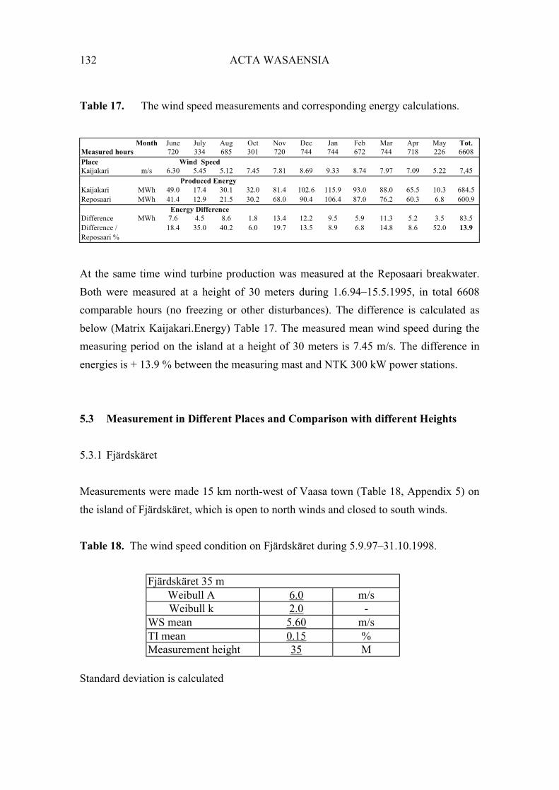
132 ACTA WASAENSIA

Table 17. The wind speed measurements and corresponding energy calculations.

Month June July Aug Oct Nov Dec Jan Feb Mar Apr May Tot.

Measured hours 720 334 685 301 720 744 744 672 744 718 226 6608

Place Wind Speed

Kaijakari m/s 6.30 5.45 5.12 7.45 7.81 8.69 9.33 8.74 7.97 7.09 5.22 7,45

Produced Energy

Kaijakari MWh 49.0 17.4 30.1 32.0 81.4 102.6 115.9 93.0 88.0 65.5 10.3 684.5

Reposaari MWh 41.4 12.9 21.5 30.2 68.0 90.4 106.4 87.0 76.2 60.3 6.8 600.9

Energy Difference

Difference MWh 7.6 4.5 8.6 1.8 13.4 12.2 9.5 5.9 11.3 5.2 3.5 83.5

Difference / 18.4 35.0 40.2 6.0 19.7 13.5 8.9 6.8 14.8 8.6 52.0 13.9

Reposaari %

At the same time wind turbine production was measured at the Reposaari breakwater.

Both were measured at a height of 30 meters during 1.6.94–15.5.1995, in total 6608

comparable hours (no freezing or other disturbances). The difference is calculated as

below (Matrix Kaijakari.Energy) Table 17. The measured mean wind speed during the

measuring period on the island at a height of 30 meters is 7.45 m/s. The difference in

energies is + 13.9 % between the measuring mast and NTK 300 kW power stations.

5.3 Measurement in Different Places and Comparison with different Heights

5.3.1 Fjärdskäret

Measurements were made 15 km north-west of Vaasa town (Table 18, Appendix 5) on

the island of Fjärdskäret, which is open to north winds and closed to south winds.

Table 18. The wind speed condition on Fjärdskäret during 5.9.97–31.10.1998.

Fjärdskäret 35 m

Weibull A 6.0 m/s

Weibull k 2.0 -

WS mean 5.60 m/s

TI mean 0.15 %

Measurement height 35 M

Standard deviation is calculated

ACTA WASAENSIA 133

(5.2) =1

N(vn

0

N

v )2

and mean Turbulence Intensity

(5.3) (TI = /v ).

In Figure 38 wind speed distribution is showed with relative frequency rf (%) and with

Weibull distribution Rf (%) with the above empirical parameters at different wind

speeds (m/s).

Fjärdskäret 35 m

0,0

5,0

10,0

15,0

1 3 5 7 9

11 13 15 17 19 21 23 25

rf (%)

Rf (%)

Figure 38. Wind speed distribution rf (%) on Fjärdskäret peninsula.

The terrain has an effect on the wind conditions. Generally the best directions for winds

are South and South West. Unfortunately to the South and South West direction there is

rising ground with forest and a high bridge (Appendix 8). An NRG wind energy

measuring anemometer and wind vane were used at the height of 35 m and at 20 m. The

German mast comparison states that it is not possible to obtain economical measuring

equipment for the wind turbine hub height. To be sure of the wind speeds, since

measuring masts reach up to 40 (50) meters in height, additional measurements were

carried out.

134 ACTA WASAENSIA

Table 19. The mean wind speeds at the Fjärdskäret measuring place.

Place, measuring moment and comparable hours Mean wind speeds

Fjärdskäret North bank 5.9.97–31.10.1998 (8860 h) 4.74 m/s 5.60 m/s

Measuring height 20 m 35 m

Table 19 values came from a matrix of (Fjärdskäret.Weibull) 8876 rows, 9 columns

and 80 000 elements such as date, hour, ws35, 35, ws20, 20, wd35, wd20, T (temperature)

(Rinta-Jouppi 1999a: 13).

5.3.2 Raippaluoto

Wind speed measurements on Raippaluoto bridge were carried out on a pylon at a

height of 83 m. An anemometer and wind direction vane were installed. The place is

about one kilometre west of the Fjärdskäret measuring mast. The measuring time was

during 10.5.– 15.7.1999 and comprised 1197 comparable hours of which 1002 hours

represented wind speed over 4 m/s.

Table 20. Measurement at the Fjärdskäret Mast and Raippaluoto Bridge Pylon.

Place 10.5–15.7.1999 Mean wind speed (m / s)

Fjärdskäret North bank 4.5 5.5 –

Raippaluoto bridge pylon – – 7.1

Measuring height (m) 20 35 83

Table 20 values came from a matrix (Fjä Rai Both) of 1201 rows, 19 columns such as

date, hour, ws83, 83, _, _, _, _, wd83, _, date, hour, ws35, 35, ws20, 20, wd35, wd20, T

(Rinta-Jouppi 1999b: 1).

ACTA WASAENSIA 135

5.3.3 Comparison to the Height

The wind speeds at the wind turbine hub height are calculated e.g. according to Walker

& Jenkins (1997: 7) with the exponent function:

(5.4) v(h2) = v(h1) *(h2 / h1)

where h1 is reference height and v(h1) reference speed, h2 is height, where v(h2) is

known and exponent describes the roughness of the surface. Another function in the

literature is a logarithmic function:

(5.5) v(h2) = v(h1)ln(h2 /z0 )

ln(h1 / z0 )

where heights h1 and h2 are the same but z0 is the roughness length. According to the

literature this means the height where the wind speed is zero. In the spreadsheet

computation table 21 the mean wind speeds at 35 m and 83 m heights are measured.

With equations 5.4 and 5.5 and z0 values are selected so that calculated and measured

values are the same at the 83 m height. will obtain in this terrain a typical iterated

value of 0,290 and z0 1,69 m. With values , z0 and the measured mean wind speed for

the whole year at 35 m 5.6 m/s the wind speed at the hub height is calculated. The result

of the mean value is 6.57 m/s at 60 m height.

Table 21. Two measuring places and two different methods to calculate hub height

wind speed.

1. h (m)

height

V (m/s)

measur.

v (m/s) yearly

measured

3. v (m/s)

calculat.

V (m/s)

measur.

h3 60 x ln (h2/z0)

h2 83 7.065 v (hz) = V (h1) --------------

h1 35 5.498 5.6 ln (h1/z0)

zo 1.69 m 3.8941121

alfa 0.290 v(83) = 5.498 --------------- 7.065 7.065

2. Alfa 3.0306195

v(hz) = v(h1)*(h/h1) v (m/s)

calculat.

V (m/s)

measur.

3.5696160

v(83) = 5.498 1.285 7.065 7.065 v(60) = 5.6 --------------- 6.60

3.0306195

v(60) = 5.6 1.1694 6.55

136 ACTA WASAENSIA

In Table 21 the measured average wind speed is at 83 m height 7.065 m/s at the top of

the pylon and at 35 m height it 5.498 m/s at the top of the mast (picture 1 in table 16).

The exponent and z0 values will be spreadsheet iterated so that the iterated and

measured wind speed at the 83 m height level are the same. With these (picture 2 in

table 14) and z0 values (picture 3) the wind speed at 60 m height will be calculated. It

gives wind speeds of 6,55 and 6,60 m/s and the mean speed 6.57 m/s. The values for

calculation came from the matrix ”Fjä Rai Both”.

Comparison to the measurements on Fjärdskäret island 5.9.1997–31.10.1998 (8860 h) at

the same place and with the same mast at 35 and 20 m heights gives by the same

calculation a wind speed at the 60 m height of 6.52 m/s (Rinta-Jouppi 1999a, in that

Appendix 18). On the reference measuring place the measured and calculated wind

speed is 6.57 m/s. The measuring mast gives after calculation 6.52 m/s. The difference

is only 0.05 m/s (0.8 %).

Next was converted, with iterated value and measured wind speeds at 35 m and 83 m

height, every wind speed to the hub heights of 60 and 67 m. The computer spreadsheet

will choose power values at different wind speeds (Appendix 9). These wind speed /

power values are given by the wind turbine manufacturer. These power values are

summed up for the whole measuring period time to energy. The same time measured

wind speeds at the 35 m height will also be converted into energy. This short time (1002

h) energy ratio has been multiplied by the whole year’s 8860 h energy production (from

NRG standard report) at the 35 m height (for example Appendix 11&12 in Rinta-Jouppi

1999b).

The additional measurement is an assumption of short term wind conditions but the

energy ratio gives a more reliable calculation base. Multiplied by a more representative

sample of wind speed data (the whole year) the difference with the calculation from the

measuring mast (Rinta-Jouppi 1999a: 15) in this case is only 0.2 % .

ACTA WASAENSIA 137

Table 22. Wind power plant production at Fjärdskäret.

Place Turbine Hub height

(m)

Wind speed

over 4 (m/s)

Capacity

factor Cf

Nominal power

operation time

(h / a)

Produced

energy

(MWh / a)

Fjärd-

skäret /

BONUS

1 MW

60 7.23 0.27 2400 2400

Raippa-

luoto

NEC Micon

1.5.MW

60 7.23 0.25 2193 3290

Nordex

1.3 MW

60 7.23 0.26 2258 2936

Vestas

V66-1650

67 7.47 0.26 2263 3735

In Table 22 the planned wind power station at Fjärdskäret is featured. The wind turbine

hub heights and wind mean speeds over 4 m/s are calculated. In addition there is the

capacity factor, which be obtained by dividing the produced energy by the turbine

nominal power and the year’s hours. The nominal power hours will be obtained by

dividing the produced energy by the nominal power, and finally the produced energy at

the hub height. The values are from the matrix (Fjä Rai Energy).

In Figure 39 wind speed differences are measured at Raippaluoto at 83 m and

Fjärdskäret at 35 m. The energy difference calculated with exponent is 0.29 at

Raippaluoto at 60 m and Fjärdskäret at 35 m height. Although the wind speed difference

is smallest in the westerly direction, the energy difference is biggest because wind

speeds are biggest from the west. The values came from the matrix (Fjä Rai Energy)

1201 rows, 19 columns, 23 000 elements such as date, hour, ws83, ws60( 0.29), wsi,

E60, _, _, wd83, _, ws35, 35, wsi, E35, wd35, wd20, _, ws, E.

138 ACTA WASAENSIA

Wind Speed Differences

0,01,02,03,04,0

N

EN E SE SS W W NN W

Directions

m/s m/s

Energy Differences

0

20000

40000

60000

N

EN E SE SS W W NN W

Directions

kW

h

kWh

Figure 39. Wind direction analysis.

5.4 Empirical Measurement on a Distant Island and Comparison to

the Measurement on the Measuring Mast onshore

5.4.1 Wind Measurements

The measurements are from fixed automatic station from the Finnish Meteorological

Institute located at Strömmingsbåda-island, about 19 km west of the Bergö measuring

mast (Appendix 5). The automatic measuring station gives, for example, a report with

place code, observation time, hourly mean wind speed and direction during the same

time period as the reference mast measurements. The anemometer and wind direction

finder is at a height of 14 meters on the beacon island. The sensors are remote-

controlled and heated if needed. Wind obstacles are the pilot house and beacon to the

north. The direction from south-east to north-west is open. The other directions are

hindered by islands (Appendix 10).

The reference measuring mast was located on Bergö island about 30 km south-west of

Vaasa (Appendix 5). The island is connected to the mainland by a ferry connection. The

measuring period was 21.11.1997–26.11.1998 (8876 h) with a 40 meter NRG

measuring mast. The mast was equipped with anemometers at 40, 30 and 20 meters and

the wind direction vane at 40 and 30 meters. In addition there was a thermometer at a

height of about 3 meters. The measuring logging unit takes a sample every second and

calculates the hourly mean value.

ACTA WASAENSIA 139

In Table 23 the mean wind speeds are measured on Strömmingsbåda island and Bergö

island fish harbour at different height levels at the same moment. 1.5 % of the total data

(9000 h) from Bergö and 0.6 % from Strömmingsbåda are rejected because of freezing

of the gauges during winter time. The values came from the matrix Bergö.B.60 and

Strömmingsbåda.G.40/60. Energy calculations were made by 1 MW power plant wind

speed/power curve.

Table 23. Mean wind speed on Strömmingsbåda and Bergö island.

Place and measuring

time 22.11.97–

26.11.1998

Measured mean wind speeds

on Bergö island

Measured and calculated Mean

wind Speeds on Strömmingsbåda

Heights (m) 20 30 40 60 14 40 60

Speeds (m/s) 5.63 6.16 6.80 7.95 6.82 8.33 9.01

Energy (MWh) - - 2563 3428 - 3687 4148

5.4.2 Sector Analysis

The energy production calculation for separate wind turbines will be made first by

selecting the comparable wind sectors (on equal terrain) in both Bergö and Strömmings-

båda. Strömmingsbåda is open from south–east to north–west. Bergö is open from south

to south–west. Table 24 describes the calculation of selected sector values. The result

has been calculated first by converting single hourly measures (8733 items) to the

desired height (from 40 m to 60 m) and then the average has been calculated. The check

column has been calculated from the average of single measures (8733 items) and

converted to the desired height.

140 ACTA WASAENSIA

Table 24. Wind direction analysis operation table.

Item Spreadsheet Calculation Operator Result Check

1 Date

2 Hour

3 Ws40 6.80 6.80

4 d40

5 Ws30 6.16 6.16

6 d30

7 Ws20 5.63 5.63

8 d20

9 Wd40

10 Wd30

11 T 4.30

12 Calc40 ws30(40/30)^(lg(ws30/ws20)/lg(30/20)) 6.60 6.56

13 Calc60 ws40(60/40)^(lg(ws40/ws30)/lg(40/30)) 7.95 7.83

14 Ws integer60 7.94

15 (360°) lg(ws30/ws20)/lg(30/20) 0.29 0.22

16 % (180-225°) 1676 19.2 %

17 Ws40 (if(wd40>180;ws40:0)*if(wd40<225;ws40;0)^(1/2) 8.66 8.66

18 Ws30 (if(wd40>180;ws30:0)*if(wd40<225;ws30;0)^(1/2) 8.13 8.13

19 Ws20 (if(wd40>180;ws20:0)*if(wd40<225;ws20;0)^(1/2) 7.71 7.71

20 Number check 1676

21 Calc40 if(ws30=0;0;ws30(40/30)^(lg(ws30/ws20)/lg(30/20)) 8.46 8.45



24 (180-225°) if(ws30=0;0;lg(ws30/ws20)/lg(30/20) 0.16 0.13

25 % (225-315°) 1497 17.1 %

26 Ws40 (if(wd40>225;ws40:0)*if(wd40<315;ws40;0)^(1/2) 7.30 7.30

27 Ws30 (if(wd40>225;ws30:0)*if(wd40<315;ws30;0)^(1/2) 6.71 6.71

28 Ws20 (if(wd40>225;ws20:0)*if(wd40<315;ws20;0)^(1/2) 6.29 6.29





33 (225-315°) if(ws30=0;0;lg(ws30/ws20)/lg(30/20) 0.19 0.16

34 % (315-22.5°) 1206 13.8 %

35 Ws40 (if(wd40>315;ws40:0)*if(wd40<22.5;ws40;0)^(1/2) 5.80 5.80

36 Ws30 (if(wd40>315;ws30:0)*if(wd30<22.5;ws40;0)^(1/2) 5.03 5.03

37 Ws20 (if(wd40>315;ws20:0)*if(wd20<22.5;ws40;0)^(1/2) 4.25 4.25





42 (315-22.5°) if(ws30=0;0;lg(ws30/ws20)/lg(30/20) 0.49 0.42

In Table 24 the measuring time was 8865 hours, 98.51 % 8733 h are acceptable hours.

values are calculated for directions 1–360°, 180–225°, 225–315° and 315–22.5°. Every

incoming wind speed is handled with spreadsheet calculation operator and the average

ACTA WASAENSIA 141

calculated for the whole group. Checking the averages is handled with the operator and

can be compared to the result. The values came from matrix Bergö.B, 8733 rows 42

columns 366 000 elements.

Table 25. Calculated values at Bergö and corresponding terrain sector at Strömb.

Terrain Bergö Strömmingsbåda

A 0.16 180–225° 135–337.5°

B 0.19 225–315° 22.5–135°

C 0.49 315–22.5° 337.5–22.5°

The exponent in formula 5.4 will be calculated with a computer spreadsheet. The data

from the Bergö measuring mast at 20 and 30 m heights give the base for exponent

calculation. For wind speeds on sector A) open sea to south to south-west (180–225

degrees) a figure of 0.16 is obtained for ( Appendix 10). The calculations for sector

B) archipelago to south-west to north-west (225–315 degrees) gives 0,19 for and

sector C) building obstacles north-west to north-east (315–22.5 degrees) 0,49.

Table 25 shows the comparable directions (wind obstacles are the same, Appendix 10).

The open sea at Strömmingsbåda is in direction A) south-east to north-north-west,

0.16. B) is the archipelago north-north-east to south-east, 0.19. C) is building

obstacles in the direction north-north-west to north-north-east, 0.49. (The values

came from matrix Bergö.B).

Table 26 exploits sector analysis of the Strömmingsbåda wind conditions. The

measured values and calculations came from the matrix Strömmingsbåda.G, 8794 rows,

26 columns and 228 000 elements.

142 ACTA WASAENSIA

Table 26. Wind speed and energy calculation at Strömmingsbåda by obtained values.

Item Spreadsheet Calculation Operator Result %

1 Date + hour

2 Ws avg 14 6.82

Wd avg 14

4 Ws60 0.38 =ws14*(60/14)^0,38 11.86

5 1–360° h 8794

6 135–330° h 4842 55 %

7 ws14 =(if(wd14>134,5;wd14;0)*if(wd14<330;ws14;0)) ^ (1/2) 7.29

8 0.16

9 ws60 =ws14*(60/14) ^ 9.21

10 15–135° h 3068 35 %

11 ws14 =(if(wd14>14,5;wd14;0)*if(wd14<135;ws14;0)) ^ (1/2) 6.52

12 0.19

13 ws60 =ws14*(60/14) ^ 8.59

14 330–15° h 884 10 %

15 ws14 =(if(wd14>329,5;wd14;0)*if(wd14<15;ws14;0)) ^ (1/2) 5.30

16 0.39

17 ws60 =ws14*(60/14) ^ 9.34

18 1–360° h 8794 100 %

19 ws60 9.01


21 E (kWh) =if(wsi60<4;0;PHAKU(wsi60;Appendix 5.2;2;0)) 401566

22 E (kWh)/month


24 E (kWh)/month


26 E (kWh)/month

Table 27. The calculated wind speeds at 60 m on Strömmingsbåda island.

Directions (degrees) 15–135 135–330 330–15 1–360

Speed (m/s) 8.59 9.21 9.34 9.01

The wind speeds are calculated at the hub height of 60 m in different directions on

Strömmingsbåda island (Table 27). The values came from matrix Strömmingsbåda.G

In the same Strömmingsbåda matrix the energy of different turbines is calculated at the

hub height and with their own wind speed / power curve (Appendix 9). The energies in

ACTA WASAENSIA 143

the above directions will be calculated together. The values will be converted from the

measuring hours minus freezing time to the calendar hours of one year.

5.4.3 Energy Calculations

The values in the wind turbine power curve are stated normally at a 15 °C temperature

and 1013,25 mbar air pressure. To change to the prevailing air density the following

formula is used (Walkers & Jenkins 1997: 11).

(5.6) P = 1/2 cp A v

3, where = 1,225 (

288

T (°K)

p(mbar)

1013,25)

and cp constant, p air pressure and T air temperature

The measured and converted values are calculated in the above equation with month

mean air temperature and pressure. With new air density the measured energy is

converted to the prevailing energy conditions.

Table 28. Measured energy converted to prevailing wind condition.

Month Meas-

ured

Temper-

ature

Air

pressure

Air

densi-

Meas-

ured

Air densi-

ty

Meas-

Ured

Air densi-

ty

Meas-

ured

Air densi-

ty

Meas-

ured

Air densi-

ty

Hours h degrees mbar Kg/m^3 energy Corrected Energy Corrected Energy corrected energy Corrected

kWh KWh KWh KWh kWh kWh kWh KWh

Bonus Bonus Vestas Vestas Nordex Nordex NEGMico NEGMico

Nov97 240 0.8 1015.8 1.292 203259 214339 222469 234596 240216 253310 129710 136780

Dec 97 741 -1.0 1013.6 1.298 733693 777120 776107 822044 890079 942762 495575 524908

Jan 98 744 -1.3 1008.0 1.292 874217 921862 921550 971775 1061416 1119264 596617 629133

Feb 98 631 -4.1 1001.9 1.297 738973 782597 777547 823448 898774 951831 505657 535507

Mar 98 741 -3.2 1012.7 1.307 763527 814590 809430 863563 923250 984995 517229 551820

Apr 98 707 0.5 1014.0 1.291 399441 420929 439275 462907 469721 494990 251708 265249

May 98 744 4.9 1014.1 1.271 486850 504967 528159 547814 578989 600535 323863 335915

Jun 98 714 9.8 1010.9 1.245 648459 658851 690477 701543 781043 793560 434672 441638

Jul 98 727 14.6 1003.3 1.215 467564 463616 508011 503722 557369 552663 309401 306789

Aug 98 744 13.9 1007.2 1.222 692026 690531 739373 737776 833595 831795 464090 463088

Sep 98 715 11.4 1014.8 1.242 702647 712630 752337 763026 843553 855538 461493 468050

Oct 98 744 7.1 1001.4 1.245 898719 913260 938358 953540 1099176 1116960 620185 630219

Nov98 602 0.4 1018.7 1.297 702678 744183 730990 774167 860967 911822 490279 519239

Altogether 8794 8312053 8619476 8834084 9159921 10038148 10410025 5600479 5808334

Years level 8760 8279916 8586151 8799929 9124506 9999338 10369777 5578826 5785878

144 ACTA WASAENSIA

The above energy values in Table 28 show the energy production on an open small

island about 30 km from land. The energy production is calculated for separate wind

turbines at 60 and 67 m hub heights. The wind conditions are nearly the same as with

real offshore turbines with the needed wind obstacle corrections. Conversion from

measured hours to calendar hours is made and from measured air conditions to wind

speed / power curve condition. (The values came from the matrix Strömmingsbådan.G

and Strömmingsbådan.V).

5.4.4 Tankar Continuous Measuring Station Assistance for Sector/Wind

Speed Analysis

There were two measuring places in Larsmo commune, Ådö and Fränsvik (Appendix

16). The idea was to measure over half a year in both places and use the whole year

continuous measuring data from the pilot house and fixed meteorological station

Tankar. So it was possible to get a whole year or more of wind speed data from the

target location, table 29 (Matrix Tankar.Ådö27Production).

The procedure: 1. A one hour average of wind speed, direction, air pressure and

temperature from Tankar (27.5 km to north east from Ådö) was asked for. 2. Then were

calculated on the same hour the wind speed differences by directions/speeds on Tankar

(h=15m) and Ådö (h=40m) over about a half years period. 3. The differences were

added to Tankar’s wind speeds. 4. Then the calculated (Ådö 40m) and right wind

speeds (Ådö 40m) were tested. 5. The measured differences was presented by a line

which is an average of measured points. The lines were calibrated so that the measured

and right wind speed differences by sector and speed class approaches zero. The same

were done with wind energy calculations. 6. The coefficients of the lines (in this case)

were used to calculate the wind speeds for the latter part of the year. In appendix 17

(matrix Tankar.Fränsvik) there is one example of measured differences and average

line. Wind speeds from 40 m were converted to the hub height 60 m. 7. The wind

speeds were converted through some turbine’s wind speed / power values to energy

values at the hub height of 60 m.

The same procedure with the measuring place Fränsvik (Tankar is 13.2 km to north east

from Fränsvik) was made.

ACTA WASAENSIA 145

Table 29. Wind conditions at Larsmo Ådö and Fränsvik at 60 m hub height.

BONUS 1MW (d54m/h60m) energy production at Ådö

Month Measured Month Mean Wind Measured Month Quarter Cf

2001 Hours h hours h speed (m/s) Energy Energy Energy

MWh MWh MWh

Jan 696 744 7.0 202.6 216.6 I/01

Feb 653 672 6.1 143.9 148.1

Mar 732 744 5.8 139.1 141.4 506.0 0.23

Apr 714 720 5.9 149.0 150.3 II/01

May 741 744 5.6 125.7 126.2

Jun 720 720 5.9 135.8 135.8 412.3 0.19

Jul 723 744 6.0 136.6 140.6 III/01

Aug 724 744 5.9 146.2 150.2

Sep 666 720 6.4 153.2 165.6 456.4 0.21

Oct 711 744 6.4 174.1 182.2 IV/01

Nov 702 720 9.6 364.6 373.9

Dec 729 744 7.1 224.5 229.1 785.2 0.36

Altogether 8511 8760 6.5 2095 2157 2160 0.25

BONUS 1MW (d54m/h60m) energy production at Fränsvik

Month Measured Month Mean Wind Measured Month Quarter Cf

2001 Hours h hours h Speed (m/s) Energy energy Energy

MWh MWh MWh

Jan 696 744 6.6 173.0 184.9 I/01

Feb 653 672 7.1 204.0 209.9

Mar 732 744 5.6 126.5 128.6 523.4 0.24

Apr 714 720 5.6 136.4 137.5 II/01

May 741 744 5.5 131.1 131.6

Jun 720 720 5.6 123.4 123.4 392.6 0.18

Jul 723 744 5.6 120.9 124.4 III/01

Aug 724 744 5.4 116.5 119.7

Sep 666 720 5.7 109.2 118.1 362.2 0.16

Oct 710 744 6.1 154.1 161.5 IV/01

Nov 701 720 9.2 327.1 336.0

Dec 686 744 6.8 196.4 213.0 710.5 0.32

Altogether 8466 8760 6.2 1919 1985 1989 0.23

146 ACTA WASAENSIA

5.5 Offshore Wind Power Plant Investment Price, Example

5.5.1 General

A solution to reduce wind electric power price is to reduce the wind turbine foundation

price. This means reducing the component, transportation and erection costs of offshore

wind parks. The industrial problem is how to develop wind power offshore foundations,

the transportation, erection and service of wind power plants. The economic problem is

to reduce the wind energy component cost compared to present day solutions. The novel

innovation WPOSFOLES (2000) is to develop a new steel foundation for power plants

and new methods to transport, erect and service the new power plants.

The main construct includes a plant foundation and power plant transport. The erection

goes, depending of the model of foundation, with an assisting modified barge or ship or

sinking the foundation alone to the sea bottom. The new type of offshore wind power

station and a modified barge facilitates the building of the wind power turbine and

foundation completely on land, transportation to the site and erection the power station

routinely. The whole idea is to make building, transportation, erection and maintenance

work easy and robust for external conditions and therefore reduce the cost significantly.

A parallel plan is to use a telescopic tower instead of a modified barge or ship. The

modified barge, ship or floating crane (Håkans 2000, Statements and Offers) keeps the

floating foundation and tower with nacelle vertical during transportation and sinking.

The telescopic tower is in a lower position (for example the nacelle at 40 m height)

during transport and floating vertically without any help. When the foundation is sunk

to the sea bottom the whole tower is lifted to the normal height.

This construct is a concept. Important questions are the strength of the combination

against wind, waves, storms, sea bottom conditions, sea currents and possible ice etc. In

realising the construct we need to examine:

– static loads

– dynamic loads

ACTA WASAENSIA 147

– fatigue loads

– corrosion

In addition we need to measure the sea bottom bearing capacity, sea flow speed, wave

height and length, possible ice effect, etc.

A weak market test for the whole construct is possible. The building of a steel

foundation is also normal workshop work (Fagerström 2000, List of Statements and

Offers). Transport and erection is normal offshore work (Håkans 2000, List of

Statements and Offers). The prices for the construct are from the above offers. A weak

market test was no longer the situation since a decision was made to start a product and

production development (Hollming 2002, list of Statements and Offers). The positive

comments from the offshore wind power market (Vestas -, NORDEX - and ENERGI

E2 A/S Interview and answer to inquiry form 2001) strengthen the standpoint that this

construct and product takes the own share of the present and future offshore foundation

and erection market and plan for tomorrow in Denmark, Germany, Sweden, Holland,

Belgium, Britain and Ireland (Appendix 14).

148 ACTA WASAENSIA

5.5.2 Foundation, calculation example

Steel/Stone/Concrete Model Weights: Hub h (m) 78Tower (t) 170Nacelle (t) 61.2Rotor (t) 37.2Total (t) 268.4

Bending (kNm) 48636

M(kNm) h(m) (TON)Hh (kN) = 48636 78 64

Floating Centre of Gravity of Mill (standing on the bottom Centre of Gravity of Mill (floating)Mass Displacement W (TON) GCi (m) Ws(TONm W (TON) GCi (m) Ws(TONm (ton) (ton) Rotor 37.2 84 3125 37.2 84 3125 1128 1128 Nacelle 61.2 84 5141 61.2 84 5141

Displacement Tower 170 45 7650 170 45 7650

depth (m) S 22 3 66 25.3 3 76 2,30 T 193 2 385 220.9 2 442

BP 368 0.25 92 613.6 0.25 153 GC (m) -------------- -------------- ------------- ------------- -------------- -------------

19,3 851 218 16459 1128 218 16587

GC (m) Centre of Gravity (floating) tan 14.7

W (ton) GC.hs (m) 5 l. y (m) M (tonm) Whole Mill 1128 14.7 0.0875 1.29 1451 Buoyancy 1128 1.15 0.0875 1.49 1678 Floating depth (m) 2.30 ./.

h(m) 78 Bending Moment (kNm) Stability 0.865 < 1 OK - M1 (TONm) = 53392 ( l(m) + H(m)) x Hh(TON) Metacentr 18.1 heigth (m)

Holding Moment (kNm) Whole mill -14.7 GC (m) - M2 (TONm) = 106402 ------------- R(m) * Weight (TON) 3.4 > 0 OK

Lift as Weight as Mass or Submerged submerged dry weight P (mk/kg) Material Work/Unit Work Totally

(TON) (TON) (TON) Area (m^2) (mk) (mk/kg. (mk) (mk) V(TON) - 268 268.4 - - Mk/m^2) - S(TON) 28 22 25.3 3.0 75917 4.00 101222 177139 T(TON) 1718 193 220.9 3.0 662766 4.00 883688 1546455

BP(TON) 245 368 613.6 0.12 73631 0.04 26998 100629 Paint(m^2) - - - 2750 - 100.00 275015 275015

----------- ----------- ---------- ----------- ------------- ---------- TON 1991 V(kN) 851 1128 812314 1286924 2099238

2633 balance(TON) Steel 246.2 1.25

268 weight TON

Water level 6 Bend.Mom Weight (kNm) Price ( )

S (TON) s1 (m) H(m) 53392 110680.03 h1(m) 4 441 333

T(TON) s2 (m) r(m) Stiffeners 1.4 Ration Ration0.016 2.1 0.50 0.57 < 1 OK

(FIM)

BP(TON) h2(m) 0.5 Bottom Hold.Mom. Lift 2 624 048R(m) 12.5 106402 19534 (kNm)

Figure 40. Spreadsheet computation simulation model for steel foundation.

ACTA WASAENSIA 149

Figure 29, 40 and Appendix 19 show the simulation model of steel/stone/concrete

foundation. Stone and concrete are on the bottom of the foundation as ballast. The wind

power plant model floats with the foundation. Foundation tanks filled with water sink it

to the sea bed. The model calculates the costs. It can optimise the costs against bending

moment (when bending moment / holding moment < 1), steel construct, stone/concrete

ballast weight and floating/sinking conditions (when mass / lift ratio < 1).

The bending moment / holding moment calculates the effect round the right down

corner of the foundation. It is dependent on the sea bottom bearing capacity where the

right rotation point is. It is calculated in figures 29 f32, 35 and ratio in g56. The floating

condition is calculated in figures 29 b47, e47, depth a21 and ratio in h56.

The centre of gravity of the mill standing on the bottom and floating is calculated in

d15-j26. The centre of gravity of buoyancy is calculated in d29-i29. It is possible to

select the inclination angle. A comparison between the whole mill moment and

buoyancy moment is made in i31. For stability inspection the metacentre point is

calculated and compared to whole mill gravity centre. This is made in zero wind speed

but gives an estimation of what the dimensions of the foundation should be.

The dry and “wet” weights are in d38-e47 multiplied with the construction required

stiffeners factor in e55.

Now we have the dimensions and can calculate the costs. In f42-45 are material costs

and painting area, in h42-45 is the work price. H42 shows the foundation “under water

tower” price, h43 the foundation price, the concrete ballast price is in h44 and the

painting price in h45. The total price in j54 is the sum in j47 multiplied with the balance

factor in j49.

The spreadsheet computation model needs 20 initial data from windmill manufacturers

and sea – and sea bed conditions for defining the foundation size and characteristics.

The foundation diameter addition (Beacon 2001) makes possible for the construction to

float without any upright keeping auxiliary vessel or crane as in the original plan. This

makes the foundation more costly but the erection is cheaper and more simple. The

price of alternatives resolves the choice.

150 ACTA WASAENSIA

Figure 40 calculates in addition the centre of gravity for the whole power plant and the

displacement of the floating construction and floating depth.

One example is the foundation itself. The foundations can be built in one place and then

floated or transported with a half-submerged barge to the harbour or dock. There the

whole power plant – the foundation, tower, nacelle, rotor and cabling and so on can be

assembled totally ready. The whole power plant will be floated, for example, on the

deck of a special half submerged barge (Håkans 2000, List of Statement and Offer). The

barge will be towed to the site. There the windmill floats from the deck of the barge.

Smaller floating or jack up type of cranes keep the windmill vertical during the

submersing of the windmill down to the sea bed.

The foundation must be constructed to keep the wind power plant in place, vertical

against wind, sea current, waves, bottom erosion and possible ice. The price of the

foundation is depends on the version and in this example is 441 333 / per unit, Figure

40.

5.5.3 Assembly, Transportation and Erection

One example is to build the foundations in Finland and transport them to Denmark, then

assemble them ready in the dock or harbour, transport them to the site floating with a

special barge, and sink the power plant on to the sea bed.

ACTA WASAENSIA 151

Table 30. The wind mill foundation transport and assembly costs.

a’ (FIM) Item Tour, men Days FIM Pieces FIM/pc /pc

Transport 38572 6487

45 000 Pori-Copenhagen 2 4 360 000 14 25714 4325

45 000 On loading Pori 1 2 90 000 14 6429 1081

45 000 Off l. Danish harbour 1 2 90 000 14 6429 1081

Harbour 62343 10485

50 000 Harbour costs 1 2 100 000 14 7143 1201

4 000 Harbour crane 1 3 12 000 1 12000 2018

2 400 Assembly work 6 3 43 200 1 43200 7266

Site 97143 16338

2 400 Site work 5 5 60 000 1 60000 10091

30 000 Material 1 1 30 000 1 30000 5046

50 000 Floating/Jack up crane 1 2 100 000 14 7143 1201

---------- --------

Altogether / unit 198058 33310

In the example in Table 30 the foundations are manufactured in Pori Finland. They are

transported to Denmark harbour / dock with the assistance of a special half-submersible

barge. They are assembled as ready power plants at the harbour. They are floated and

erected at the site with the assistance of a small crane.

5.5.4 Cabling

In the example the wind power park is 20 km offshore and onshore there is a sufficient-

ly strong 20 kV line. The cable and cable let down work costs 40 / m (Rinta-Jouppi

1995: 25). The Tunö Knob park cable onto land 10 kV 6 km costs 1.5 M$. The local

ring between turbines 10 kV 2,8 km costs 0.6 M$.( 2.6 km land cable 0.4 M$). With

exchange rate 1$ = 6.45 DKK and 1 = 7,4288 DKK (14.2.2002) it costs 217 /m, 186

/m and 133 /m (Morthorst et al. 1977: 203 and Madsen 1996: 5). 110 kV 3 km 3

MFIM amounts to 168 /m (Holttinen et al. 1998: 109) On the sand bed it is possible to

use a pressured water spray to get the cable into the sand bed. The cabling can be

152 ACTA WASAENSIA

surprisingly expensive 11.47 M / 12.8 km makes 896 /m (http://www.middelgrunden.

dk/MG_UK/project_info/prestudy.htm 2000, p. 10).

The material and work costs of a 20 000 m cable is with item price 160 /m 3.2 M . If

the distance between the 14 turbines is 300 m/each, it makes (13 x 300 m) 3900 m.

Totally 23 900 m and with 160 /m multiplied it makes 3.824 M . For 14 turbines it

makes 273 143 /turbine. Every turbine has its own 20 kV transformer.

5.6 Operation and Maintenance Costs

The operation and maintenance costs include many different items, see Chapter 2.4.3.

For older turbines the O&M cost can be 3 per cent and bigger turbines 1.5–2 % of the

original turbine investment. Wear and tear on the turbine generally also increases with

increased production. The used value for O&M is 0.01 $/kWh. The research centre

ISET has analysed 250 MW wind power stations during 10 years. 500-600 kW plants

costs are 30 DEM/kW. It makes 1,5 % of the investment price of 1000 /kW. Finnish

research states 5–10 FIMp/kWh (Tammelin et al. 2001). Morgan et al. (2001: 2–37) say

as much as 30 % of energy cost and for 95 % availability £ 30 000 per turbine. Svenson

et al. (1999: 298) use for the calculation 0.01 /kWh.

5.7 Offshore Wind Power Price, Example

As an assistance construct the price of electric power is calculated. As an example a

wind power plant park 20 km from shore is used with a sufficiently strong 20 kV line.

There are 14 turbines and the distance between the turbines is 300 m (Chapter 5.5.4, the

cabling cost 3.824 M ). The transport barge takes the 14 turbine foundations and the

same amount of ready assembled power plants to the site (Table 30, 33 310 / pc). The

year production comes from Chapter 5.4.3, Table 28 – energy calculations. The other

information needed for the calculations comes from the literature, manufacturer’s bid,

foundation, steel construction, assembly, transport and erection, sea bed research and an

interview. The operation and maintenance cost come from Chapter 5.6. The capital

ACTA WASAENSIA 153

costs are calculated with 5 % real interest and the lifetime is 20 years. Tande (1994: 23)

recommends levelled correction factors for annual power production during year t:

Kper,t 1.00 Performance factor (rain, dirt, etc.)

Ksite, t 0.95 Site factor (obstacles)

Kava, t 0.95 Technical availability factor (failure, service)

Klos, t 0.95 Electrical transmission losses factor

Kutil, t 1.00 Utilisation factor

Total 0.86

In Table 31 the energy price at Strömmingsbåda is calculated. There are turbine

characteristics, onshore bid prices, offshore calculated prices, total investment costs,

O&M cost, levelled years production and production cost. Depending on the turbine the

kWh price varies from c 3.60 to 4.70. (Table comes from matrix c per

kWh.Strömmingsbåda).

The best kWh prices are between c 3–4, depending on the wind turbine. Turbine B has

over large bending moment and that effects large and expensive foundation. That is to

seen in the kWh price. It is far higher than the old water power price, on the level of c

1, but below new coal and nuclear power prices (Figure 17 OECD 1993 prices for

separate production methods).

154 ACTA WASAENSIA

Table 31. Kilowatt price of different wind turbines.

Kilowatt Price with separate Power Plants

Measuring Periode on the Strömmingsbåda and Bergö Islands on 22.11.97 - 26.11.1998

Producer Turbine A Turbine B Turbine C Turbine D Rated Power (kW) 2 000 1 500 2 500 2 000

Rotor D(m) 76 64 80 80

Hub Height h(m) 80 60 80 78

Weight (TON) 270 203 310 268

Onshore Bid Prices Wind Turbine ex works 1 495 000 100 % 1 309 452 100 % 1 758 100 % 1 717 200 100 %

Transport to Dock 10 000 0.7 % 10 000 0.8 % 10 000 0.6 % 10 000 0.6 %

Transformer 30 000 2.0 % 30 000 2.3 % 30 000 1.7 % Incl.

Remote Control 3 500 0.2 % 2 528 0.2 % Incl. Incl.

Training incl. incl. 10 226 11 500

Accessory 40 000 2.7 % incl. 98 398 5.6 % 6 100 0.4 %

Warranty Time's Service 40 000 2.7 % 11 840 0.9 % incl. Incl.

Altogether 1 618 500 108 % 1 363 820 104 % 1 906 108 % 1 744 800 102 %

Currency Factor 1.00000 1.00000 1.00000 1.00000

Turbine on Dock 1 618 500 1 363 820 1 906 1 744 800

/ kW 809 909 763 872

Offshore Calculated Prices Steel Foundation 331 959 22.2 % 329 251 25.1 % 378 524 21.5 % 319 508 18.6 %

Transport 6 487 0.4 % 6 487 0.4 % 6 487 0.4 % 6 487 0.4 %

Harbour/Dock Assemblage 10 485 0.7 % 10 485 0.8 % 10 485 0.6 % 10 485 0.6 %

Site Work 16 338 1.1 % 16 338 1.2 % 16 338 0.9 % 16 338 1.0 %

Sea-bed Reseach 20 000 1.3 % 20 000 1.5 % 20 000 1.1 % 20 000 1.2 %

Cabling (20+3.9 km, 160 /m, 14 273 143 18.3 % 273 143 20.9 % 273 143 15.5 % 273 143 15.9 %

Planing 10 000 0.7 % 10 000 0.8 % 10 000 0.6 % 10 000 0.6 %

Additional Charge 10 000 0.7 % 10 000 0.8 % 10 000 0.6 % 10 000 0.6 %

Total Investment 2 296 912 153.6 % 2 039 524 155.8 2 631 149.7 % 2 410 761 140.4 %/kW 1 148 1 360 1 053 1 205

Investment 0 % 0 0 0 0

Net Investment 2 296 912 153.6 % 2 039 524 155.8 2 631 149.7 % 2 410 761 140.4 %

/kW 1 148 1 360 1 053 1 205

Operation and Maintenance ( /year) Operation and Maintenance 73 616 4.9 % 49 607 3.8 % 88 908 5.1 % 78 231 4.6 %

Insurance 15 000 1.0 % 15 000 1.1 % 15 000 0.9 % 15 000 0.9 %

Administration 5 000 0.3 % 5 000 0.4 % 5 000 0.3 % 5 000 0.3 %

Altogether ( /year) 93 616 6.3 % 69 607 5.3 % 108 908 6.2 % 98 231 5.7 %

O&M ( c/kWh) 1.27 1.40 1.22 1.26

Year Production (kWh/a) 8 586 151 5 785 878 10 369 9 124 506Levelised Utilized Energy (0.86) 7 361 551 4 960 667 8 890 7 823 123

Year Production per Swept Area 1 623 1 542 1 769 1 556

Nominal Power Time (h/a) 3 681 3 307 3 556 3 912

Capasity Factor (Cf) 0.42 0.38 0.41 0.45

Production Cost ( c/kWh) 3.78 4.70 3.60 3.73

Real Interest 5 % Refund Periode 20 Year 2 000 1 500 2 500 2 000

Swept Area (m^2) 4 536 3 217 5 027 5 027

ACTA WASAENSIA 155

5.8 Summary

The main and assistance construct is presented in chapter 3. It is tested with the method

presented in Chapter 4 and the results are presented in Chapter 5.

The results are developed to obtain the electricity price in a model of a wind turbine

park located some ten kilometres from shore (in this example, off Strömminsbåda). The

main work is done with spreadsheet matrices and the results are presented in Chapter 5.

The construct example results are presented in Chapter 5.5.2. The spreadsheet

calculation allows the feeding of all size turbine, tower height, water depth and to a

certain extent the sort of sea bottom; in total 11 initial values concerning foundation

features. These give:

– the foundation price

– sufficient bending / holding moment

– sufficient floating features

– centre of gravity

– centre of buoyancy

and possibly

– floating stability without external assistance (ship or barge) tower in

the telescope mode

The assembly, transportation and erection example costs are presented in Table 30. The

operation and maintenance costs are from the literature. In Table 31 all data are

connected to the kilowatt price with separate wind turbines off Strömmingsbåda in a 14

turbine wind park.

156 ACTA WASAENSIA

0,000

0,050

0,100

0,150

0,200

0,250

0,300

0,350

0,400

0,450M

BendingM

Wlevel

TurbineW

Stiffeners

WorkPrice

BendingM 0,275 0,290 0,304 0,320 0,343 0,362 0,387

Wlevel 0,310 0,313 0,316 0,320 0,323 0,326 0,329

TurbineW 0,325 0,328 0,325 0,320 0,322 0,320 0,320

Stiffeners 0,240 0,266 0,293 0,320 0,346 0,373 0,399

WorkPrice 0,274 0,289 0,304 0,320 0,335 0,350 0,365

0,7 0,8 0,9 1,0 1,1 1,2 1,3

-30 % -20 % -10 % 0 % 10 % 20 % 30 % Variation

Figure 41. Sensitivity analysis: The effectiveness of various cost components on

foundation price. (Note decimal points commas not dots)

The sensitivity analysis (Figure 41 Matrix SensitiveAnalysis.Vestas2MW) tells that the

most price increasing component is Stiffeners coefficient. It tells how much steel is

needed to use for construction against static and dynamic (fatigue) load. The second

most price increasing component is the wind turbine manufacturer stated bending

moment. It describes wind conditions e.g. gust happening over 50 years. The construc-

tion shall tolerate these. The bending moment is depending e. g. on rotor diameter,

wings form and how they can be turned to the wind direction. The work price has an

effect on third place. Water depth and turbine weight do not affect much when the

variation is between -30 – +30 %.

ACTA WASAENSIA 157

6. EVALUATION OF THE RESULTS AND RESEARCH METHODS

6.1 General

This study attempts to clarify the costs and cost structures of wind power production,

especially the costs that are caused by the logistic factors of location and erection of

offshore wind power stations, and proposes one possible solution.

Table 32. Evaluation of the costs of new construction and state-of-the art of

technology (Table 8 and 9, Appendix 12, Middelgrunden 2000: 11,12 and

Sörensen 2002).

Item New Construct

(the Research)

State-of- the Art of Technology

(Middelgrunden 2000) Sörensen (2002)

Foundation Fig. 39 331 959 393 500 496 000

Transport Tab.25 6 487

Harbour Tab. 25 10 485

Site Tab.25 16 338 100 500 134 500

Other costs Tab. 26 A 40 000 60 000 80 500

Sum Tab. 26 A 405 269 554 000 711 500

In Table 32 the prices of the two same kinds of foundations (gravity based) are

compared. The cost of new logistic construction is calculated in Table 31. The right

prices of state-of–the art–technology are most difficult to obtain – for understandable

reasons – but in Appendix 12 the prices are calculated. Middelgrunden 2000 prices are

budget prices but according to the tender. For example, total costs are in Middelgrunden

2000 m 46.95, Eskesen 2001 gives cost of m 49.2 and Sörensen m 44.9.

A typical saving for a 20 mill park could be m 2.97 – 6.12.

158 ACTA WASAENSIA

The foundation prices are on the same level. The new construct requires transport and

harbour payment. The site work shows a difference. The main saving is to avoid the use

of offshore cranes. Other costs are on the same level.

Benefits also come by another route. In summer months is possible to use offshore

crane 50 % of the time and during the year 10 % of the time. The costs are round 133

000 per day independent of sea conditions (Vestas 2001, Håkans 2000 list of

statements). It makes the budgeting of costs very unstable, too.

The costs of offshore park size vary as follows: the turbine and cable between turbines

stays on the same level between park size from 2 to 200 MW or more. The cable is e.g.

20 kV and the length between turbines 3–5 x rotor diameter. In the larger parks the

turbines are in rows and the distance between rows is 5 – 9 x rotor diameter. The cable

prices are in chapter 5.5.4. The total cabling price, however, depends very heavily on

sea bottom conditions. According to Morgan & Jamieson (2001: 2–46) transmission

price depends on three possible options:

a) multiple medium voltage links (up to 35 kV) for parks some kilometres offshore

and size less than 200 MW

b) single high-voltage link (100 to 200 kV) for longer distance offshore and larger

wind parks

c) HVDC (High Voltage Direct Current) link for parks above 25 km offshore and

power level more than 200 MW

In addition the shade effect of the park should be considered. There can be a 28%

production loss in unidirectional wind with turbulence intensity of 0.05 and in omni

directional case with turbulence intensity of 0.15 a 5 % production loss, depending on

the distance of the turbines and rows with 10 rotor diameter (Lissaman 1998: 305).

The results will be appraised by clarifying the effectiveness of wind power electricity

price against the cost and production components. In Figure 42 the components are

calculated on Stömmingsbåda wind conditions at the 60 meter hub height with 1 MW

turbine. In this example the wind turbine technical and commercial data are used to

simulate turbine electricity production. The example uses a 14 wind mill turbine park at

a 20 km distance from land and 3.9 km cables between the 1–1.65 MW turbines (Annex

ACTA WASAENSIA 159

12) and sandy sea bottom. The price consists of cost of investment (interest and

lifetime) and operation & maintenance costs divided by electricity production. In this

sensitivity analysis the parameter variation factors are 0.7, 0.8, 0.9. 1.0, 1.1, 1.2, 1.3.

In Appendix 11 (Matrix c Sensitivity Analysis.Strömmingsbåda60m) one of the five

cost factors changes and the other stays constant. For every varied cost factor the

corresponding electricity price ( c/kWh) is calculated and can be seen in Figure 42.

Figure 42. Sensitivity analysis: The effectiveness of various cost components on

electricity price. (Note decimal points are commas not dots)

For varied wind speeds the wind turbine corresponding power is taken from the curve

and calculated with a year’s production. The total year’s cost and the year’s production

are divided by cost per energy ( c/kWh). The same is as in figure 42 (Matrix Sensitivity

Analysis.Strömmingsbåda60m), which shows the effectiveness of cost components with

the electricity price. The variation for different components is shown in the graph.

160 ACTA WASAENSIA

It is clearly seen that the most important factor is the mean wind speed. Changes in

wind speed measurement, calculations and estimates influences most on the energy

price. The other components have an effect but are not as strong factors as wind speeds.

6.2 Validity

Validity refers to the ability of a measure to measure what it is intended to measure.

Internal validity establishes a causal relationship, whereby certain conditions are shown

to lead to other conditions, as distinguished from spurious relationships. In this study

such a measure is not applicable (Yin 1994: 35).

External validity considers to which domain the result or findings from a study can be

generalised. The method handled in Chapter 6.3.1 could be generalised. If it is possible

to find equal wind conditions in separate places, with this method it is possible to

transfer the measurement results to another place. The foundation construct’s validity

depends on the sea bottom structure. If the bottom is solid and smooth the research

construct is valid. In other cases other foundations come into question (such as mono

pile) or levelling the sea bottom (for example concrete planes) (Yin 1994: 36).

6.2.1 Construct Validity

In term of construct validity, the question here is whether the research is constructed to

produce the cheapest wind power? Other possibilities are, for example, wind turbines

located high in the mountains. There wind speeds are favourable. On the other hand

transport to the site can be difficult and at the height of clouds there is freezing on the

blades at air temperature below zero Celsius. Ice on the blades can be avoided by using

a heating system. This research in any case is evaluating the lowest possible price at sea.

The selected construct is right if it leads to the result wanted.

ACTA WASAENSIA 161

6.2.2 Wind Speed

The sensitivity analysis in figure 42 shows the most important components of the wind

power price. According to Lange & Höjstrup (1999: 1166) and Rinta-Jouppi (1995 in

there appendix 17.2 and 17.3), the wind speed accelerates away from the shore and 10

km away from the shore is 1–2 m/s more than on the coastline at the same height. The

measurement on Bergö and measurement of Finnish Meteorological Institute data from

Strömmingsbåda (Table 23) shows that the measured mean wind speed already on

Strömmingsbåda at a 14 m height (6.82 m/s) is higher than on the coastline at a 40 m

height (6.80 m/s). The figures from Strömmingsbåda (8.33 m/s) island, 30 km from the

coastline and 19 km from Bergö (6.80 m/s) show a calculated 1.53 m/s higher wind

speed than both at the same 40 m height level. The conclusion is that at sea the wind

blows more than at the coastline. Kühl (1999: 47) has collected the statistics from

different wind parks, wind speed by separate hub height and distance from land (Table

33). The wind speeds above are in line with statistics collected from the North sea and

the Baltic sea.

Table 33. Wind speed at different hub heights and the distance from the shore.

Name of Project or Study Wind speed(m/s) Hub Height (m) From Shore(km)

Vindeby, Baltic, DK, P-91 7.5 37.5 1.5

Lely,North Sea, UK, P-94 7.7 41.5 1.0

Tunö Knob,Baltic, DK, P-95 7.5 43.0 6.0

Horns Rev, NS, DK, S-97 9.2 55.0 15.0

Bockstiegen-Valar, B, SE P-

97

8.0 41.5 4.0

6.2.3 Investment

According to Table 31 the investment price depends on the turbine, transport to the

dock, the transformer, remote control, training, accessories, warranty, steel foundation,

162 ACTA WASAENSIA

transports, harbour/dock assemblage, site work, sea-bed research and cabling, etc. With

planning and additional charges it costs, depending on the turbine, 1.05–1.36 M / MW.

Svenson & Olsen (1999: 299) and Appendix 12, have studied parks at Rödsand, Omö

and Dedser using steel foundations with olivine ballast and calculated with 1.5 MW x

96 turbine parks per each site. They decided the total investment to be 1.46–1.65 M /

MW.

This research calculates the foundation is at a 6 meter water depth. The cost of founda-

tion depends on turbine weight, bending moment, hub height, water depth, diameter and

height of tower and foundation, steel thickness, stone/concrete ballast, painting and

stiffeners. In total 11 starting values for spreadsheet computation define the outer and

inner measures of the foundation and construct (Figure 40). The cost of foundation

(Table 31) in these four calculation examples are 331 959, 329 251, 378 524 and 319

508 . The Svenson & Ohlsen (1999: 297) research gives for steel construction at a 5–

11 meter water depth a price of 265 000–318 000 for 1.5 MW turbines (Appendix 12).

6.2.4 Interest and Lifetime

The practice of using 5 % real interest and 20 year life time makes comparison easier

with different cost figures in references. 5 % interest is in practise very near reality

because when the interest on bank loans is higher than 5 %, inflation starts to increase

and the real interest is again 5 %. A 20 year lifetime is an economical lifetime. Modern

wind turbines have not yet reached a 20 year lifetime, so it is not possible to say how

long the construct lifetime actually is.

However, if wind turbine production costs and electricity selling prices rise equally as

much (Table 34) it is possible to use real interest in the calculations. Statistical yearbook

1999 shows the rise of production and electricity prices. From 1980 to 1998 the rise for

all the index is about double. The wholesale electricity price follows the rise quite

exactly since in 1979 the index was 575, rising after a year to 737.

ACTA WASAENSIA 163

Table 34. Statistical yearbook; electricity selling and production prices.

Year 392.31b Wholesale

price index; gas,

electricity and heat

392.7 Wholesale price

index; machinery and

transport equipment

393.7 Production price

index; machinery and

transport equipment

1980 737 971 810

1998 1228 1899 1655

The conclusion is that inflation has caused a doubling of electric power price and the

same rise in wind turbine production price during the same period (Table 34) and if the

rise in future follows the same track, we can generally use real interest. It means that

bank interest minus general inflation stays constant and in this special branch earning

and costs follow each other. By using real interest the calculation becomes notably

easier because it is not necessary to discount future development of earnings and costs

to this day. The established real interest by wind power calculations is 5 %/a. In Finland

during 1989-1998 the average rates of interest on advancing minus cost of living index

change was on average during that time 6.337 %/a. At the same time the average rates

of interest on advancing minus wholesale price index change was an average 7.25 %/a

(Statistical Yearbook 1999: 250 and 387).

6.2.5 Operation and Maintenance

In the literature the figure for O & M costs including operation, maintenance, insurance

and administration is 0.01 $ / kWh (Chapter 2.4.3). The research of Svenson & Olsen

(1999: 299) uses 0.011 / kWh. Earlier some percentage of the total investment price

was used, then some percentage of turbine investment. Now the figure is calculated

from produced energy, which may best reflect use and wear and therefore future costs

also. Offshore O&M costs are higher than onshore wind turbines. Offshore windmills

are difficult to reach because of waves, sea current and wind compared to the O&M of

windmills on land. There the service vehicles can drive right up to and beside the

windmill.

164 ACTA WASAENSIA

Verbruggen et al. (2001) calculate the following values for offshore wind farms

operation and maintenance costs. These figures in Table 35 are very near to the earlier

presented figures.

Table 35. Operation & Maintenance costs.

Type of maintenance Annual cost ( /kWh)

Preventive maintenance 0.005–0.012

Corrective maintenance 0.010–0.019

6.3 Reliability

Reliability refers to the consistency of measurement results, including such characteris-

tics as accuracy and precision. Reliability demonstrates that the operations of the study

such as the test data collection procedures can be repeated, with the same results

(Olkkonen 1994: 38).

Validity focuses on the meaning and meaningfulness of data. Reliability focuses on the

consistency of results (Sykes 1991: 309).

6.3.1 Wind speed

The most reliable wind speed is possible to obtain only by measuring with a mast at hub

height with a heated anemometer. For example on Strömmingsbåda island the

measuring gauges on the mast must be at the windmill hub height at 60 m. Using

computer simulating methods and measurements with lower masts makes the research

more uncertain. The calibration of the anemometers and different wind years must be

taken into consideration, too. In this research the wind speed measuring has been

completed from Bergö island reached by car with a 40 meter mast and at the same time

19 km to the west with a time series at 14 meters. The results have been converted to 60

meter hub height.

ACTA WASAENSIA 165

Bergö Strömmingsbåda

315°

0.39

22.5°

225°

180°

0.16

0.19

330°

0.39

15°

135°

0.16

0.19

Figure 43. The same values in different places and sectors.

According to the literature the wind speed accelerates when the height increases

according to the formula (4.1). The Bergö 40 meter mast has anemometers at heights of

20, 30 and 40 meters. In the above formula potency will be calculated at the above

directions. The selected wind directions on Bergö correspond to wind obstacles on

Strömmingsbåda island. With corresponding values in Figure 43 the 14 meter height

statistics are converted to 60 meter wind speed. The directions 15º–135º–330º–15º will

be calculated. The corresponding mean wind speeds are 8.59, 9.21, 9.34 m/s and for all

directions the mean speed is 9.01 m/s (Table 27). The energy calculations are made in

the same manner selecting from the whole 8794 hours statistics with the same wind

speeds at the above directions and taking the corresponding power values of the wind

turbine and adding to the energy of the above directions. The obtained energy from the

selected directions will be added together for whole 360º energy.

The method is tested in Chapter 4.1.4 (Reference Measurements on Height Direction)

by using the top of the bridge pylon for the anemometer. The distance between the two

measuring places was one kilometre.

166 ACTA WASAENSIA

The anemometer calibrations are made in a wind tunnel defining the wind speed shown

by the anemometer. If there is difference between the real and anemometer values, this

is taken into consideration in the calculations.

Whether the measuring year has been a good or bad wind year it must be estimated for

example, with statistics from the Finish Meteorological Institute of Valassaaret island,

53 km to the north east of Strömmingsbåda (Appendix 13). In the years 1961–1990 the

mean wind speed has been 6.6 m/s and at the same place and in the same measurement

environment. During the time of this research the wind speed has been 5.9 m/s (Rinta-

Jouppi 1999a: 9). The conclusion is that the coming years will be more windy.

6.3.2 Investment

The investment example consists of a) onshore up dated bid prices (Table 31) and b)

offshore calculated prices (Table 30).

The steel foundation cost consists of (Figure 40) materials such as steel, ballast stone/

concrete, paint and also work: the amount and price. The wind turbine manufacturer

defines the data of the turbine consisting of tower, engine room and rotor weight,

bending moment, diameter and plate thickness of tower, and so on.

Figure 40, which is at the same time a spreadsheet program, calculates with the given

values the diameter, height and ballast of the foundation so that the whole wind turbine

bending/holding moment is under 1. In the same manner the weight / lift will be under

1. This means that the whole construct floats when the water tank is empty and the

version in Figure 40 floats alone without assistance of smaller crane to keep the turbine

on a vertical position (List of Statement and Offer: Beacon 2001). With ballast the

turbine stays vertical against wind, sea current, waves and ice in the sea bottom. In the

calculations the material and work amounts and prices used are inspected by an SME

(Small and Medium size Enterprise) owner, who calculates and produces equal steel

components (WPOSFOLES 2000, List of Statement and Offers: Fagerström 2000). The

simulating program allows the combining of the measures and masses to find the lowest

price for the foundation.

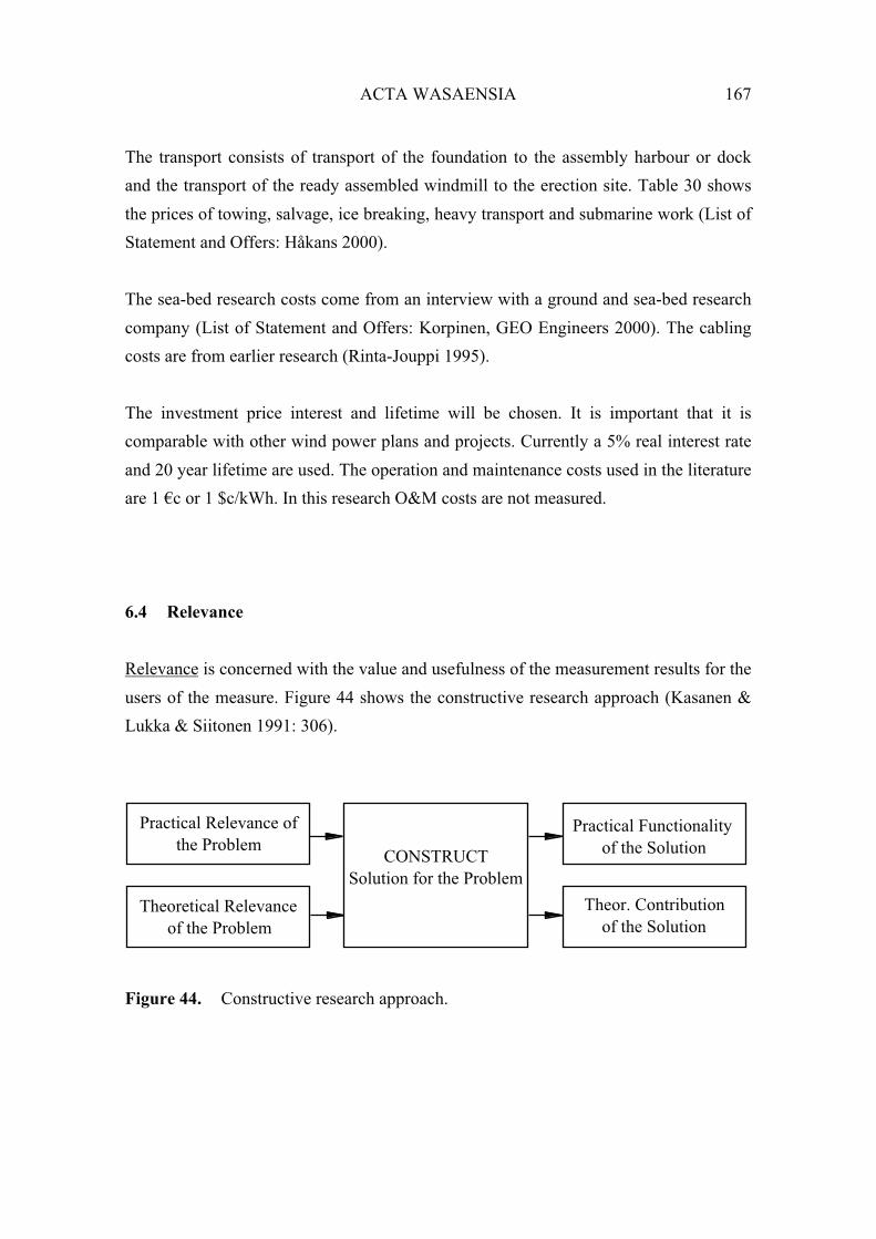
ACTA WASAENSIA 167

The transport consists of transport of the foundation to the assembly harbour or dock

and the transport of the ready assembled windmill to the erection site. Table 30 shows

the prices of towing, salvage, ice breaking, heavy transport and submarine work (List of

Statement and Offers: Håkans 2000).

The sea-bed research costs come from an interview with a ground and sea-bed research

company (List of Statement and Offers: Korpinen, GEO Engineers 2000). The cabling

costs are from earlier research (Rinta-Jouppi 1995).

The investment price interest and lifetime will be chosen. It is important that it is

comparable with other wind power plans and projects. Currently a 5% real interest rate

and 20 year lifetime are used. The operation and maintenance costs used in the literature

are 1 c or 1 $c/kWh. In this research O&M costs are not measured.

6.4 Relevance

Relevance is concerned with the value and usefulness of the measurement results for the

users of the measure. Figure 44 shows the constructive research approach (Kasanen &

Lukka & Siitonen 1991: 306).

Practical Relevance of

the Problem

Theoretical Relevance

of the Problem

CONSTRUCT

Solution for the Problem

Practical Functionality

of the Solution

Theor. Contribution

of the Solution

Figure 44. Constructive research approach.

168 ACTA WASAENSIA

The practical relevance could be wind measuring at the measuring points on the map,

Appendix 5. The theoretical relevance could be the research of offshore windmill

electricity prices, going far offshore as the planned wind parks are. Figure 34 and 42

show that wind speed is the most important component of the price. Therefore

theoretical relevance is to take measurement at the site of a planned park with a

measuring mast at a hub height over several years. Practical relevance gives the

possibility of use: measuring with a 40 meter mast on land and converting FMI (Finnish

Meteorological Institute) data from a beacon island from a 14 meter height to hub

heights. The evaluation of whether the measuring year was a good or bad wind year can

be done by comparing wind data over a 30 year period from a nearby measuring station.

The practical functionality of the solution of the whole construct is to develop

competitive electric power. The wind speed and the other cost components define the

whole construct competitiveness.

The theoretical contribution of the solution follows Porter’s 1985 theory of reaching

cost leader status. This means reaching a low cost level compared to competitors. The

solutions in reaching low level costs are in going out to sea far enough, e.g. by more

than 20 km from the shore and selecting the park location in shallow water from 5 to 15

meters in depth, ideally a place on the sea without ice, sea current, big waves and with a

hard, smooth sandy sea bottom. To be a cost leader in electric power price the price of

the foundation of the windmill should be on the limits shown in Figure 40 for steel

foundation. The foundation prices in Table 31 are from 18.6 % to 25.1 % of the turbine

price itself and the total investment is from 140.4 % to 155.8 % of the turbine (including

tower) price (31,4 % foundation and 196 % total investment, Barthelmie et al. 2001: 6–

3, 17.6 % foundation and 170 % total investment, Fuglsang & Thomsen 1998: 13). The

electric power prices are shown in the same table. The comparison to other production

methods is in Figure 1. and to other park locations in Appendix 12. This construct does

not take into consideration investment support, return of taxes or other subsidies. It

means that all figures are real costs without subsidies.

ACTA WASAENSIA 169

6.5 Practicality

The practicality is defined as the benefit-burden ratio of measurement. In other words,

are the measurement results worth the effort needed for the implementation and the

maintenance of the measurement. The measures are needed to get exact figures con-

cerning wind power price components, the local wind speeds. The possibility to esti-

mate wind speed by computer simulated program is too risky for big investments. To

win cost leader status the foundation solution must include new ideas to obtain cheaper

construction, transport and erection. Cost leader status includes the whole work

practicality. If the whole working process is not practical, the process can not be a cost

leader.

6.6 Summary

Does this research construct lead to the cheapest wind power electricity during the

turbine life time? In this research we do not inspect possible mountain sites and wind

speeds and wind power there. In this construct wind speeds are mapped offshore.

Foundations suitable for offshore site, assembly, transport, cabling and erection on site

are included in this research. The construct produces cheaper wind electricity but not yet

at the same level as water power electricity. The best wind conditions and the cheapest

foundation, transport, erection, cabling, and O&M leads to cost leader position.

170 ACTA WASAENSIA

7. CONCLUSION

7.1 Summary of Construct Created

The created construct brings new knowledge to the question of the direction in which

the wind power plant industry and wind turbines should go. The computer simulated

foundation model and also the small scale foundation with turbine model bring new

knowledge to this branch of science. The unique computer simulated foundation model

brings the right dimensions and solutions to the foundation in different conditions of sea

and sea bottom and also to the different scales and types of wind turbines. A wind

turbine foundation which floats and stays filled with water on the sea bottom leads the

construct to cost leader position (Porter 1985) among the foundation structures. The

example foundation used requires minimum values for foundation diameter 25 m,

height 4 m, 0.5 m high concrete ballast and cost 441 333. The typical saving can be

2.97 – 6.12 M for a park of 20 turbines). To sell the electric energy produced by

windmills seems to be difficult if the produced energy is not at the same price level with

other electricity production. The power plant produces wind electricity of 3.73 c/kWh

with cost of 1.2 M /MW with wind speed of 9 m/s at 60m height.

This research construct helps in two ways to reach a lower wind electricity price level.

The location of the windmill parks, in this case, are offshore, about 20 km from the

coast. The wind speeds are significantly higher there than nearer the coast and on the

coastline. A rough estimation is that the offshore wind speed level is 15 % higher than

onshore winds. The theoretical power formula P = 1/2 Av

3 promises 50 % more energy.

The reason to go offshore is the better wind speed. It is measured in two places on

Kaijakari 0.5 km from land on an island. The measured energy was 13.9 % better than

onshore on a breakwater. The other case Strömmingsbåda is 19 km out to sea. The wind

speed difference at 40 m height is 22.5 % and energy difference 43.8 %. At 60 m height

the differences are for the wind speed 13.3 % and energy 21.0 %. This can be due to

land effect; the forest does not so much affecting the wind speed at 60 m height.

ACTA WASAENSIA 171

Mean wind speed difference at 60 m height is 1.06 m/s Strömmingsbåda/Bergö. The

formula (5.6) shows that the power increases by the potency of three when the wind

speed increases by the first potency (In practice the potency is some decimals points

above two). In practice often a half meter per second increase or decrease of wind speed

at the planned turbine location decides if the place is good or bad for wind power

production. This reason can result in a positive or negative cash flow for the wind

electricity producer. Another reason to go offshore is practical. The lack of suitable

places for wind turbines on shore is even worse in so called wind power countries.

The other solution to lead the construct into cost leader position is a unique logistical

system to fabricate, transport, assemble and erect the foundation and the connection of

windmill hull, engine room and rotor. The construct brings to the market a solution

which significantly affects further constructs and price level. The whole construct

brings wind electric power to a competitive position with other electric producer plants.

For example with the operation time of 5000h/a the production costs are for peat 38.25

/ MWh, gas 29.63 / MWh and coal 29.42 / MWh and on Strömmingsbåga location

for wind power 37.3 /MWh.

7.2 Applicability of the Results

In the previous chapter we described the construct influencing the electric power price.

The basis for competitive wind electricity price is the measurement of wind speeds on

Bergö, Fjärdskäret and at the top of the Raippaluoto bridge pylon and also earlier

measurements on Kaijakari (Chapter 5). Those data and analyses bring understanding of

how the wind behaves on and offshore at separate heights and on different terrain. The

most important cost component of wind power is the wind speed (20% smaller mean

wind speed increases the wind electric price from 4.7 to 9.5 c/kWh).

The unique test for the formula and spreadsheet applications is included in the

calculation of wind speed at the hub height. The measuring mast measures wind speeds

at heights of 30 and 20 m. On the basis of this data we can calculate the 60 m height

172 ACTA WASAENSIA

speed. To control the result we use the pylon height of 82 m and 30 m data to calculate

the 60 m speed. The results are very close. This formula can thus be used.

The other unique measuring and calculation is to convert the Strömmingsbåda island

Finnish Meteorological Institute data from a 14 m height to 60 m height wind speed. On

Bergö island, 20 km east, the measuring mast measured the wind speeds at 40, 30 and

20 m heights. From this data we can calculate in different directions with the formula

(5.4) potency factor. The potency factor always varies according to wind obstacles.

Now we can select the same obstacle conditions for the measuring mast and conditions

on Strömmingsbåda island: mainly sea, a similar archipelago and similar obstacle

(building) by selecting the right sectors of a 360º circle. With this the potency factor

we calculated the wind speeds from 14 m data to 60 m data.

7.3 Contribution of the Research

The contribution to the science of this branch is a unique type of foundation for the

offshore wind turbine. A new logistical system to fabricate, assemble, transport and

erect offshore wind turbines is a contribution to the economy of wind electricity

production. These measurements of wind speeds and calculations of offshore conditions

will increase the internationally rather rare measurements and knowledge of wind

speeds ten kilometres from the coast at the windmill hub height. All the results of this

research lead to the goal of obtaining more competitive wind electric power compared

with other power plants and for manufacturers to find more economic ways to produce,

transport, assemble and erect wind parks in offshore locations For one foundation,

turbine transportation and assembly in the harbour and floating to the site and assembly

on the sea bottom cost 33 310.

7.4 Need for Further Research

A need for further research would be for wind measuring masts directly at windmill hub

height. Currently fabricated masts can be carried by hand on the terrain, and it is

ACTA WASAENSIA 173

possible to erect them in places where no vehicle can go. They are also possible to erect

and unload in a day or two. Today’s portable measuring masts are 40 (50) m high and

hub heights are 60 m and higher. It should be possible to erect on land or in the middle

of sea at the hub height and the data could be read by radio signals.

In Ådö and Fränsvik (Chapter 5.4.4 Appendix 16, 17) the researcher attempts to

continue the measuring after the measuring mast is taken down with the help of a fixed

weather station nearby. The verification for method used is still missing.

There is still a great lack of wind energy measurements in inland Finland, on the sea

coastline and offshore. Wind measurements have been made already for at least a

hundred years but for the purpose of weather forecasts and warnings for sea navigators.

These measurements serve badly in terms of wind energy data.

Still more questions arose during the research work. On the basis of earth surface

friction the wind direction turns by rising to an upper level. Could the alteration of wind

course be used to calculate the wind speed at an upper level?

If on any business branch there are some turnover figures, how much does it employ

people with subcontract chains down to the excavation of raw material?

The foundation itself needs detailed planning, static and dynamic load calculations,

drawings, verifying small scale analysis, status in the market, detailed price calculations

and comparisons with comparable solutions in the market, as well as the mapping of

subcontractors such as tug-boats, crane contractors and cabling.

Considering historical data over the range of machine sizes, the cubic scaling law

regarding system masses and costs appears closer to a square law with ongoing

technology development (Morgan & Jamieson 2001: 2–13).

In general we need to research what possibilities (offshore) wind power really offers in

terms of replacing other electricity production in the whole country or part of it. What

is the price of the replacement? To estimate the price in the future we need to take into

consideration the super-fast development of wind power plants and wind power turbine

174 ACTA WASAENSIA

manufacturing (from the eighties to the present the power of a single wind turbine has

doubled during each 3 or 4 year period, from 30-40 kW to 2,5 MW).

ACTA WASAENSIA 175

REFERENCES

Bade, P. & B. Sundermann (1996). Der Wind. In: Windkraftanlagen, 93–119. Hrsg. Robert

Gasch. Stutgart: B.G. Teubner. 390 p.

Band, Erster (1970). Statik flüssiger und gasförmiger Körper. In: Dubbel, Taschenbuch für den

Maschinenbau, 289–292. Springer-Verlag Berlin. 959 p.

Barthelmie, R. & S. Frandsen (2001). Economics and Financing. In: Offshore Wind Energy.

Ready to Power a Sustainable Europe. Supported by the European Commission.

Report Ref.: 2001.006.

BTM Consult ApS – March (2001).

De Witt, Ubbo & Wilfried Hübner (1996). Technische und ökonomische optimierung eines

windparks. Windkraftanlagen. Hrsg. Robert Gasch. Stuttgart: B.G. Teubner. 390 p.

DEA/CADDET (2000). Electricity from Offshore Wind. Danish EnergyAgency and IEA

CADDET Renewable Energy Programme, ETSU, Harwell UK, Delft University

Wind Energy Research Institute (Duwind).

DEWEK '94, Wilhelmshaven, Windenergie-Konferenz, Deutsches Windenergie-Institut GmbH

– DEWI. 11.2.2010504. 479 p.

DWTMA (Danish Wind Turbine Manufacturers Accociation) (1998). Offshore Wind Power

Research. Available: www.windpoer.dk/tour/rd/offintro.htm.

Finnish Aeronautical Association (1968). Lentäjä ja sää. Helsinki: Suomen Ilmailuliitto. 138 p.

Frost, Walter & Carl Aspliden (1998). Characteristics of the Wind. In: Wind Turbine

Technology, 371–446. Ed. David A. Spera. New York: The American Society of

Mechanical Engineers. 638 p.

Fuglsang, Peter & Kenneth Thomsen (1998). Cost Optimization of Wind Turbines for Large-

Scale Offshore Wind Farms. Roskilde, Denmark: Risö National Laboratory,

February 1998. 30 p.

Gasch, R & J. Maurer (1996). Auslegung von Windturbinen nach Betz und Schmitz. In:

Windkraftanlagen, 120–151. Ed. Robert Gasch. Stutgart: B. G. Teubner, 390 p.

Grusell, Gunnar (1995). A Model for Calculating the Economy of Wind Power Plant. In: EWEA

Special Topic Conference on the Economics of Wind Energy, 52–57. Helsinki,

EWEA '95, Finnish Wind Power Association. 245 p.

Haapanen, Erkki (1998). Perustus. In: Offshore-tuulivoima Perämeren jääolosuhteissa. Ed.

Hannele Holttinen. Espoo: Valtion Teknillinen Tutkimuskeskus. 118 p. +

Appendices.

Haapanen, Erkki (1972). Aerodynamiikka. Helsinki: The Finnish Aeronautical Association. 102

p.

Hannula, Mika (1999). Expedient Total Production Measurement. TTKK.

176 ACTA WASAENSIA

Hartel, G. & D. Milborrow (2000). Prospects for Offshore Wind Energy, BWEA Report to the

EU Altener Contract XVII/4.1030/Z/98–395), London.

Holttinen, Esa & Jari Keinänen (1998). Pohjois-Pohjanmaan rannikon tuulivoimakartoitus –

Teknistaloudelliset tarkastelut. Espoo: Energia-Ekono Oy, 59 p. + Appendices.

Holttinen, Hannele (1998). Jalustatyypit, kustannukset. In: Offshore-tuulivoima Perämeren

jääolosuhteissa. Ed. Hannele Holttinen. Espoo: Valtion Teknillinen Tutkimuskeskus,

103 p. + Appendices.

Kasanen, E., K. Lukka & A. Siitonen (1991). Konstruktiivinen tutkimusote liiketaloustieteessä.

In: The Finnish Journal of Business Economics 3, 301–325.

Krohn, Sören (1998) Guided Tour on Wind Energy. Danish Wind Turbine Manufacturers

Association. Available: http//www.windpower.dk/tour/wres/shear. htm.

Krohn, Sören (1998) Offshore Wind Power Research. Danish Wind Turbine Manufacturers

Association. Available: http//www.windpower.dk/tour/rd/offintro. htm.

Krohn, Sören (1998) Operation and Maintenance Costs for Wind Turbines. Danish Wind

Turbine Manufacturers Association. Available: http//www.windpower.dk/tour/

econ/oandm.htm.

Krohn, Sören (1998).Offshore Wind Energy: Full Speed Ahead. Danish Wind Turbine

Manufacturers Association.

Kühn, M. et al. (1998). Structural and Economic Optimization of Boom-Mounted Offshore Wind

Energy Converters. JOR3-CT95-0087 Institute for Wind Energy, Delft University of

Technology, Delft.

Kühn, Martin (1999). Don’t Be Fooled by Theoretical Offshore Potential. In: New Energy 1,

46–47. Osnabrück: German Wind Energy Association. 58 p.

Laitinen, E. (1992) Yrityksen talouden mittarit. Jyväskylä: Gummeruksen Kirjapaino Oy. 377 p.

Lange, Bernhard & Jörgen Höjstrup (1999). WASP for Offshore Sites in Confined Coastal

Waters – the Influence of the Sea Fetch. In: 1999 European Wind Energy

Conference, 1165–1168. London: James & James (Science Publisher) Ltd. 1244 p.

Lemming, Jörgen (1997). The Danish 4000 MW Offshore Programme. In: Proceedings of

European Wind Energy Conference EWEC97, 37–42. Irish Wind Energy

Association, Slane, County Meath, Ireland. 847 p.

Madsen, Peter Stenvald (1996). Tunö Knob Offshore Wind Farm. In: Proceedings of European

Comminity Wind Energy Conference OCWEC’96, 4–7. H.S. Stephens & Associates,

UK.

Middelgrunden (2000). 40 MW Offshore Wind Farm, a Prestudy for the Danish Offshore 750

MW Wind Programme.

Middelgrunden Wind Turbine Co-operativa (2000). Available: Middelgrunden.dk/MG_

UK_info/prestudy.htm. 14 p.

ACTA WASAENSIA 177

Milborrow, David (1997). Costs, Prices and Values. In: Wind Energy the Facts, 63–91.

Luxembourg: Office for Official Publications of the European Communities, 1999.

231 p.

Morgan, C.A. & P. Jamieson (2001). Offshore Technology. In: Offshore Wind Energy. Ready to

Power a Sustainable Europe. Supported by the European Commission.

Morthorst, P.E. & L. Schleisner (1997). Offshore Wind Turbines – Wishful Thinking or

Economic Reality. In: Proceedings of European Wind Energy Conference EWEC97,

201–205. Irish Wind Energy Association, Slane, County Meath, Ireland. 847 p.

Mäkinen, Saku (1999). A Strategic Framework for Business Impact Analysis and Its Usage in

New Product Development. TTKK.

Määttänen, Mauri (1998) Perustustekniikat. In: Offshore-tuulivoima Perämeren jääolosuhteissa,

66–69. Ed. Hannele Holttinen. Espoo: Valtion Teknillinen Tutkimuskeskus, 103 p. +

Appendices.

New Energy (1/2001). Installed Wind Power Capacity, p. 44. Osnabrück: German Wind Energy

Association. 52 p.

NRG MicroSite (1996). MicroSite, User’s Guide. User Manual. Hinesburg USA: NRG

Systems, Inc.

Olkkonen, T. (1993). Johdatus teollisuustalouden tutkimustyöhön. HUT Report No 152.

Helsinki University of Technology, Helsinki, Finland.

Olkkonen, Tauno (1994). Johdatus teollisuustalouden tutkimustyöhön. 2. Ed. Espoo: TKK

Offset. 143 p.

Peltola, E. & J. Petäjä (1993). Tuulivoima Suomen Energiahuollossa. VTT Julkaisuja 775.

Espoo.

Porter, Michael E. (1980). Competitive Strategy. Helsinki: Oy Rastor Ab. 431 p.

Porter, Michael E. (1985). Competitive Advantage, 201–205. Espoo: Weiling & Göös. 648 p.

Reisman, A. (1988). On Alternative Strategies for Doing Research in the Management and

Social Sciences. IEEE Transactions on Engineering Management 35:4, 215–220.

Rinta-Jouppi, Y. (1992). Tuulivoiman koelaitos Poriin. NEMO raportti. Satakunnan

Teknologiakylä Oy. 15 p. + Appendices.

Rinta-Jouppi, Y. (1995). Luodolle sijoitettu offshore tuulipilotlaitos. NEMO2 raportti. Pori:

PrizzTech Ltd, Technology Center. 32 p. + Appendices.

Rinta-Jouppi, Y. (1998). Tuulivoimaloiden offshore rakentaminen. Engineering Office

Kustannussalpa Ltd, Tekes publication.

Rinta-Jouppi, Y. (1999a). Tutkimus taloudellisesti kannattavan tuulivoiman edellytyksistä

Vaasan rannikkoseudulle. Loppuraportti; BotniaWind. Oy Merinova Ab / Innowest.

22 p. + Appendices.

178 ACTA WASAENSIA

Rinta-Jouppi, Y. (1999b). Tutkimus taloudellisesti kannattavan tuulivoiman edellytyksistä

Vaasan rannikkoseudulle. Lisämittauspöytäkirja; BotniaWind. Oy Merinova Ab /

Innowest.

Satakunnan Kansa (21.7.2000). Tuulivoima saanut hyvän vastaanoton. Pori: Satakunnan Kansa.

Savolainen, Ilkka & Seppo Vuori (1999) Energia ja ympäristö. In: Energia Suomessa, 128–168.

Ed. Mikko Kara. Helsinki: Oy Edita Ab. 368 p.

Smith, Bernie et al. (2001). Social Aspects. Final Raport: Concerted Action on Offshore Wind

Energy in Europe. In: Offshore Wind Energy, Ready to Power a Sustainable Europe,

Chapter 8. Main author Bernie Smith. Netherlands: European Commission/Delft

University of Technology.

Sommardal, T., H. Holttinen, B. Lemström & E. Peltola (1994). Tuulivoimalaitoksen

sijoittaminen luodolle. VTT tiedotteita 1572. Espoo: Technical Research Centre of

Finland. 58 p.+ Appendices.

Spera, David A. (1998). Introduction to Modern Wind Turbines. In: Wind Turbine Technology,

47–72. Ed. David A. Spera. New York: The American Society of Mechanical

Engineers.

Statistical Yearbook (1999). Statistics Finland. Helsinki. 677 p.

Surugiu, L & I. Paraschivoiu (1999). Acceptability, Environmental and Social Aspects of Wind

Energy. In: 1999 European Wind Energy Conference, 586–589. London: James &

James (Science Publisher) Ltd. 1244 p.

Svenson, Jan & Frank Olsen (1999). Cost Optimising of Large-scale Offshore Wind Farms in

the Danish Waters In: 1999 European Wind Energy Conference, 294–299. London:

James & James (Science Publisher) Ltd. 1244 p.

Sykes, Wendy (1991). Validity and Reliability in Qualitative Market Research: a Review of the

Literature. In: Journal of the Market Research Society 32:3.

Tammelin, Bengt, Folke Malmgren & Esa Holttinen (2001). Tuulivoiman käyttökustannukset

alle Bronsin. Tekniikka & Talous 1.3.2001. Helsinki.

Tammelin, Bengt (1991a). Suomen Tuuliatlas. Helsinki: Ilmatieteen laitos. 356 p.

Tammelin, Bengt (1991b). Meteorologista taustatietoa tuulienergiakartoitukselle. Helsinki:

Ilmatieteen laitos. 332 p.

Tammelin, Bengt (1999). Offshore tuulivoimaa, pp. 23. Tuulensilmä. 3. Helsinki: Suomen

Tuulivoimayhdistys ry. 36 p.

Tande, John Olav & Raymond Hunter (1994) 2. Estimation of Cost of Energy from Wind

Energy Conversation Systems. Roskilde: Risö National Laboratory, DK 4000

Roskilde, Denmark & Glasgow: Renewable Energy Unit, East Kilbridge, Glasgow

G75 0QU, United Kingdom. 32 p.

Tarjanne, Risto & Sauli Rissanen (2000). The Nuclear Option. In: Energy in Finland 2000, 18–

19. Ed. Ilkka Leppä. Helsinki: ETY-Lehdet Oy. 114 p.

ACTA WASAENSIA 179

Walker, John F. & Nicholas Jenkins (1997) Wind Energy Technology. West Sussex UK: John

Wiley & Sons. 161 p.

Valtanen, Esko (1994) Koneenrakentajan taulukkokirja. Jyväskylä: Teknolit. 785 p.

Vandenbulcke, Luc (2001). The Utgrunden Wind Farm Project and Future Evolutions. In: Ewea

Conference Offshore Wind Energy. Brussels Belgium CD-ROM.

Verbguggen, Theo et al. (2001). Maintenance Manager to Control Operation and Maintenance

of Offshore Wind Farms. In: EWEA Special Topic Conference on the Offshore Wind

Energy, 10–12. December 2001 (CD-ROM).

WPOSFOLES (2000). A Patent FI 107184. Helsinki: Patentti- ja Rekisterihallitus. 12 p.

180 ACTA WASAENSIA

LIST OF STATEMENTS AND OFFERS

Beacon Finland Ltd Oy (2001). (Naval Architects & Marine Consultants) A Computer

Fine Element Analysis of Structure.

BONUS Energy A/S (1998). Budgetary Prices for 1 MW Turbine and up to Date

Information for 2 MW Turbine.

Dansk Vindmölleformidling (2001).

ENERGI E2 A/S (2001). Interview and Answers to Inquiry Form.

Fagerstöm, Asko (2000). Foundation Workshop Manufacturing. Asteka Oy. Heavy

Steel Work and Installations to Oil Drilling and Paper Industry, Pori.

Hollming Oy, Licence Agreement and Written Opinion.

Håkans, Joakim (2000). Transportation from Pori to Front of Kopenhagen Alfonso

Håkans (Towage – Salvage – Icebreaking – Heavy Transport – Submarin

Work, Turku).

Korpinen, Tapani (1999). Sea-bed Research Costs. Geo Engineers Oy. Ground

Research etc. Pori.

NEG Micon A/S (1998). Information and Prices for 1.5 MW Turbine.

NORDEX A/S (2001). Interview and Answers to Inquiry Form.

NORDEX A/S (1998). Relevant Information and Prices for 1.3 MW Turbine and up to

Date Information for 2.5 MW Turbine.

Vestas A/S (2001). Interview and Answers to Inquiry Form.

Vestas Wind Systems A/S (1998). Information and Prices for 1.65 MW and up to Date

Information for 2MW.

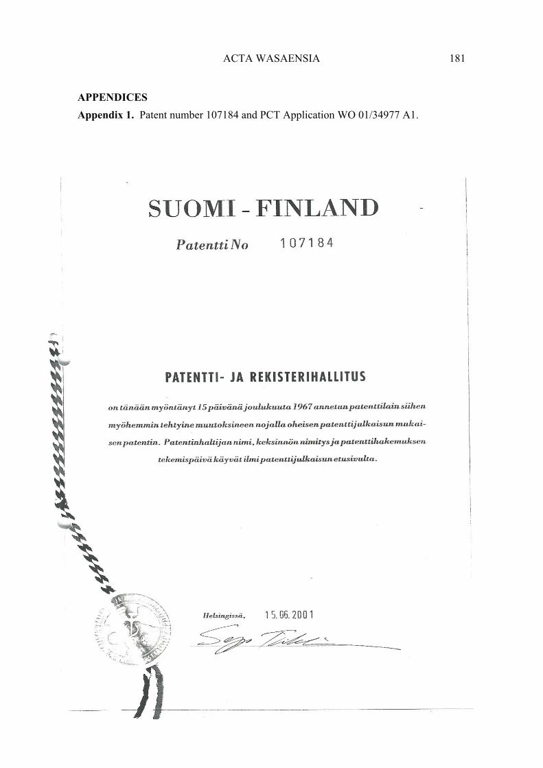
ACTA WASAENSIA 181

APPENDICES

Appendix 1. Patent number 107184 and PCT Application WO 01/34977 A1.

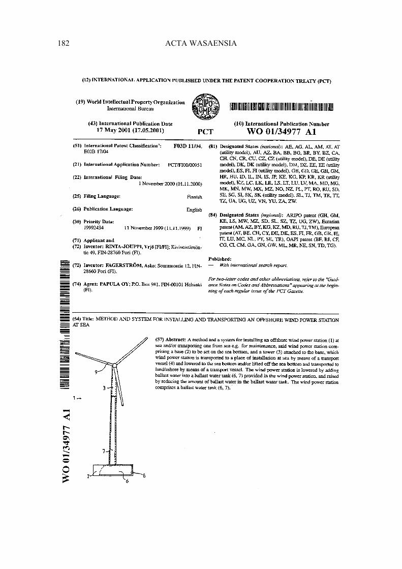
182 ACTA WASAENSIA

ACTA WASAENSIA 183

METHOD AND SYSTEM FOR INSTALLING AN OFFSHORE WIND POWER STATION

AT SEA AND/OR TRANSPORTING ONE FROM SEA, AND AN OFFSHORE WIND

POWER STATION

The present invention relates to a method as defined in the preamble of

claim 1. Moreover, the invention relates to a system as defined in the

preamble of claim 7. In addition, the invention relates to an offshore wind

power station as defined in the preamble of claim 11.

In prior art, a method for installing an offshore wind power station at

sea is known from specification GB 2327440. The wind power station comprises a

wide base and a tower extending vertically from the base and carrying a wind

rotor mounted on its top. In the installation method presented in the above-

mentioned specification, the tower and the base of the wind power station are

transported as a single assembly by using a floating frame, e.g. barges,

fastening the base to the bottom surface of the barge, transporting it to the

place of installation and then lowering it to the sea bottom using means

provided on the floating frame, such as chains, wire cables, a lever jack or

the like. The floating frame can then be used for the installation of other

corresponding base tower combinations.

A problem with this prior-art method is that the load capacity of the

floating frame used for installation has to be so designed that it will bear

the weight of the base and tower in addition to its own weight. The resulting

floating frame is very bulky and expensive. Besides, this specification

completely neglects the occasional need to raise the wind power station from

the sea bottom and transport it to land/ashore for servicing. .With equipment

built according to the specification, this would be difficult if not

impossible because the base, which may be made of concrete or steel, must be

very heavy to resist the stress exerted on the wind power station by the wind,

sea currents, waves and ice. Therefore, the base is provided with ballast

material of sand, stones or iron ore. Lifting such a load from the bottom

requires very high external hoisting capacity. Therefore, special open sea

crane ship would be needed for the hoisting operation.

The object of the invention is to eliminate the above-mentioned

drawbacks.

A specific object of the invention is to disclose a method and system for

the transportation of an offshore wind power station that will allow

transportation without the transport vessel having to carry the weight of the

wind power station at all.

A further object of the invention is to disclose a wind power station

which can be easily transported back and forth between a place of installation

and a place of maintenance and which can be raised and lowered independently

in water without using any special hoisting equipment.

184 ACTA WASAENSIA

The features characteristic of the method, system and wind power station

of the invention are presented in the claims below.

In the method of the invention, the wind power station is transported to

a place of installation at sea by using a transport vessel and lowered to the

sea bottom and/or raised from the sea bottom and transported to land/ashore by

means of a transport vessel. According to the invention, the wind power

station is lowered by adding ballast water into a ballast water tank provided

in the wind power station- and the wind power station is raised by reducing

the amount of ballast water in the ballast water tank.

In the system of the invention, the wind power station comprises a base

to be mounted on the sea bottom, a tower attached to the base, and a transport

vessel provided with a gripping device for gripping the wind power station and

transporting the wind power station to a place of installation at sea and/or

transporting it to land/ashore from the sea. According to the invention, the

system comprises a ballast water tank disposed in the wind power station.

The offshore wind power station of the invention comprises a base to be

mounted on the sea bottom, and a tower attached to the base. According to the

invention, the wind power station comprises a ballast water tank.

Other preferred features and embodiments of the invention are presented

in the sub claims below.

In the following, the invention will be de

scribed in detail by the aid of a few examples of its 15 embodiments

with reference to the attached drawing, wherein

Fig. 1 presents an embodiment of the wind power station of the invention

in a diagrammatic side view and partly sectioned,

Fig. 2–7 present two different embodiments of the system of the invention

and different stages in the procedure of the invention.

Fig. 1 presents a wind power station 1 according to the invention. It

comprises a wide base 2 of e.g. a round slab-like shape, which can be set on

the sea bottom. Further, the wind power station comprises a tower 3 attached

to the base and extending vertically from it. Mounted on the upper end of the

tower 3 is a wind rotor 9. The box-like base 2, which may be made of concrete

or steel, is of a hollow construction and the space inside it functions as a

ballast water tank or container 6. The tower 3 is likewise of a hollow

construction and the space inside it serves as a ballast water tank 7. The

interior spaces of the ballast water tanks 6, 7 in the base 2 and tower 3 may

ACTA WASAENSIA 185

be separate spaces or they may communicate with each other. Moreover, the wind

power station 1 may comprise a pump or pumps 8, by means of which it is

possible to pump sea water into and out of the ballast water tanks 6, 7. The

pump 8 may also be disposed on a transport or service vessel 4, in which case

the wind power station need not necessarily be provided with ballast water

pumps.

The buoyancy of the wind power station in water is so designed that the

station is able to float and carry its own weight in water when the ballast

water tanks 6, 7 are empty. Correspondingly, when the ballast water tanks 6, 7

are partially or completely filled with water, the wind power station will

sink to the bottom.

In Fig. 2, the base 2 and the tower 3 are assembled on land or ashore into a unitary whole

by using a crane ashore. The base 2 can be floated separately to the place of installation and

lowered onto a firm pedestal resting on the bottom by filling the ballast water tank 6 in the base. On

the top of the

base 2, a tower 3 is built from one or more parts. Water can also be

pumped into the ballast water tank 7 in the tower to increase its firmness.

Finally, a machine room and a wind rotor 9 are mounted on the end of the tower

3.

When the wind power station is to be transported to its place of

installation at sea, as illustrated in Fig. 3 and 4, the amount of ballast

water in the ballast water tanks 6 and 7 in the base 2 and in the tower 3 is

so adjusted that the base 2 becomes buoyant and is lifted off the bottom. By

adjusting the amount of ballast water in the tank 6, 7, the elevation and

stability of the base in relation to the transport vessel 4 are adjusted to

make them suitable for transportation. The tower 3 is gripped from a lateral

direction from opposite sides by the gripping jaws 10 of a gripping device 5

mounted on the transport vessel, as illustrated in Fig. 4. The grip on the

tower is preferably such that it permits movement of the tower in a vertical

direction in relation to the transport vessel but not in other directions. The

win- power station is then transported to its place of installation at sea.

Fig. 5 and 6 illustrate an alternative solution for implementing the

transport vessel in Fig. 3 and 4. In Fig. 5 and 6, the transport vessel 4 used

is a barge 4 having a forked frame with a through slot 11 extending from its

middle to the edge, allowing the tower 3 to go through the slot. For

transportation, the base 2 can be fastened in a substantially fixed manner to

the barge 4. The upper surface of the base 2 lies against the bottom of the

barge 4 and is fastened to it by suitable fastening elements 12, such as wire

cables chains, threaded bolts or the like.

Fig. 7 presents a phase in the procedure at which the wind power station

has been brought to the place of installation and an amount of water

sufficient to increase the weight so as to allow the base 2 to sink to the sea

bottom has been pumped into the ballast water tank 6 of the base 2 and into

the ballast water tank 7 of the tower 3.

186 ACTA WASAENSIA

Substantially the entire inside space of the tower 3 constituting the

ballast water tank 7 can be filled with water. Providing a ballast water tank

in the tower 3 in addition to the base 2, together with an appropriate design,

enables the weight of the wind power station to be increased so that it can

rest very firmly on the bottom and the wind power station is able to receive

the loads generated by wind, sea cur rents, sea roll and ice, which tend to

upset or move the wind power station. Furthermore, providing a ballast water

tank 7 in the tower 3 makes it possible to use a base 2 of a relatively light

and compact construction.

The base 2 can be provided with water jet equipment (not shown in the

figures) , by means of which the bottom, if it is e.g. of a sandy nature, can

be dredged after the base has sunk against the bottom thus making it possible

to adjust the vertical alignment of the wind power station.

When the wind power station is to be brought ashore from the sea for

maintenance, the procedure is naturally reverse to that for installation. The

amount of water in the ballast water tanks 6, 7 of the wind power station 1

standing on the bottom is reduced until the buoyancy of the base 2 and tower 3

has lifted the station off the bottom and raised it to a level near the

surface. Via the ballast water tank 6, 7, the elevation and stability of the

wind power station are adjusted to make them suitable in relation to the

transport vessel 4 used for transportation. The tower 3 is then gripped from

opposite sides by the gripping device 5 of the transport vessel 4 and the wind

power station is transported away from the place of installation to a place of

maintenance.

The invention is not restricted to the examples of its embodiments

described above; instead, many variations are possible within the scope of the

inventive idea defined in the claims.

CLAIMS

1. Method for installing an offshore wind power station (1) at sea and/or

transporting one from sea e.g. for maintenance, said wind power station

comprising a base (2) to be mounted on the sea bottom. and a tower (3)

attached to the base, which wind power station is transported to a place of

installation at sea by means of a transport vessel (4) and lowered to the sea

bottom and/or lifted off the sea bottom and transported to land/ashore by

means of a transport vessel, c h a r a c t e r i z e d in that the wind

powerstation is lowered by adding ballast water into a ballast water tank (6,

7) provided in the wind power station and that the wind power station is

raised by reducing the amount of ballast water in the ballast water tank.

ACTA WASAENSIA 187

2. Method as defined in claim 1, c h a r a c t e r i z e d in that

vertical motion of the wind power station (1) in relation to the transport

vessel (4) is permitted during the transportation.

3. Method as defined in claim l or 2, c h a r a c t e r i z e d in that,

to install the wind power station at sea, the wind power station is gripped by

a gripping device (5) mounted on the transport vessel (4) ; the elevation and

stability of the wind power station are adjusted by the aid of the ballast

water tank (6, 7) to make them suitable with respect to the transport vessel;

the wind power station is transported to the place of installation at sea and

the wind power station is lowered at the place 0= installation to the sea

bottom by filling the ballast water tank (6, 7).

4. Method as defined in claim l or 2, c h a r a c t e r i z e d in that,

to transport the wind power station from sea, the amount of water in the

ballast water tank (6, 7) is reduced until the wind power station has risen

off the bottom to a level near the surface; using the ballast water tank

(6,7), the elevation and stability of the wind power station are adjusted to

make them suitable in relation to the transport vessel (4) ; the wind power

station gripped by the gripping device (5) of the transport vessel (4) ; the

wind power station is transported ashore from the place of installation, e.g.

to a place of maintenance; and the wind power station is released from the

grip of the transport vessel.

5. Method as defined in anyone of claims 1-4, c h a r a c t e r i z e d

in that a ballast water tank (6) disposed in the base (2) of the wind power

station is used, and/or that a ballast water tank (7) disposed in the tower

(3) of the wind power station is used.

6. Method as defined in anyone of claims 1-5, c h a r a c t e r i z e d

in that the tower (3) of the wind power station is gripped by the gripping de-

vice (5) of the transport vessel (4) from opposite sides.

7. System for installing an offshore wind power station (1) at sea and/or

transporting one from the sea e.g. for maintenance, said wind power station

comprising a base (2) to be set on the sea bottom, and a tower (3) attached to

the base, and a transport vessel (4) provided with a gripping device (5) for

gripping the wind power station to transport it to a place of installation

at sea and/or from the sea to land/ashore, c h a r a c t e r i z e d in that

the system comprises a ballast water tank (6, 7) disposed in the wind power

station.

8. System as defined in claim 7, c h a r a c t e r i z e d in that the

system comprises a pump (u; disposed on the vessel (4) 'or on the wind power

station (1) for pumping ballast water into/out of the ballast water tank (6,

7)

9. System as defined in claim 7 or 8, c h a r a c t e r i z e d in that

the base (2) is provided with a ballast water tank (6) and/or that the tower

(3) is provided with a ballast water tank (7).

188 ACTA WASAENSIA

10. System as defined in anyone of claims 7 - 9, c h a r a c t e r i z e

d in that the gripping device (5) of the transport vessel comprises gripping

jaws (8) for gripping the tower (3) from a lateral direction from its opposite

sides, said gripping jaws being designed to allow vertical motion of the tower

in relation to the transport vessel (4).

11. Offshore wind power station comprising a base to be set on the sea

bottom and a tower (3) attached to the base, c h a r a c t e r i z e d in that

the wind power station comprises a ballast water tank (6, 7).

12. Offshore wind power station as defined in claim 11, c h a r a c t e r

i z e d in that the base (2) is provided with a ballast water tank (6) and/or

that the tower (3) is provided with a ballast water tank (7).

13. Offshore wind power station as defined in claim 11 or 12, c h a r a c

t e r i z e d in that the wind power station (1) comprises a pump (8) for

pumping ballast water into/out of the ballast water tank (6, 7).

(57) ABSTRACT

A method and a system for installing an offshore wind power station (1)

at sea and/or transporting one from sea e.g. for maintenance, said wind power

station comprising a base (2) to be set on the sea bottom, and a tower (3)

attached to the base, which wind power station is transported to a place of

installation at sea by means of a transport vessel (4) and lowered to the sea

bottom and/or lifted off the sea bottom and transported to land/ashore by

means of a transport vessel. The wind power station is lowered by adding

ballast water into a ballast water tank (6, 7) provided in the wind power

station, and raised by reducing the amount of ballast water in the ballast

water tank. The wind power station comprises a ballast water tank (6, 7).

ACTA WASAENSIA 189

190 ACTA WASAENSIA

ACTA WASAENSIA 191

Appendix 2. Sensitivity Analysis on Fjärdskäret.

192 ACTA WASAENSIA

Appendix 3. Wind Measuring and Analysis Equipment.

ACTA WASAENSIA 193

Appendix 4. Pori Kaijakari Measuring Locations.

194 ACTA WASAENSIA

Appendix 5. Measuring Places Strömmingsbåda, Bergö, Fjärdskäret and Valassaaret.

ACTA WASAENSIA 195

Appendix 6. Production statistics at different places in Finland during the measuring

time (Tuulensilmä nr 4/2002).

196 ACTA WASAENSIA

Appendix 7. Calculation Example with Turbine Power 1–1.65 MW.

ACTA WASAENSIA 197

Appendix 8. Fjärdskäret Measuring Location.

198 ACTA WASAENSIA

Appendix 9. Wind speed / Power values for different Turbines.

ACTA WASAENSIA 199

Appendix 10. Measured values at Bergö and corresponding values at Strömmings-

båda.

200 ACTA WASAENSIA

Appendix 11. Sensitivity Analysis for 2 MW turbine in Strömmingsbåda Wind

Conditions.

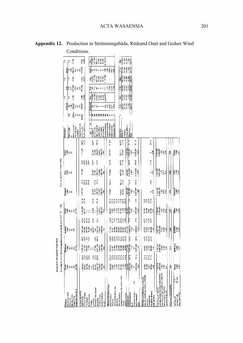
ACTA WASAENSIA 201

Appendix 12. Production in Strömmingsbåda, Rödsand Omö and Gedser Wind

Conditions.

202 ACTA WASAENSIA

Appendix 13. Monthly and Annual Wind Speeds in Mustasaari Wind Conditions.

ACTA WASAENSIA 203

Appendix 14. Planned and tentative Wind Farms (Concerted Action on Offshore

Wind Energy in Europe 2001: 9–26).

204 ACTA WASAENSIA

ACTA WASAENSIA 205

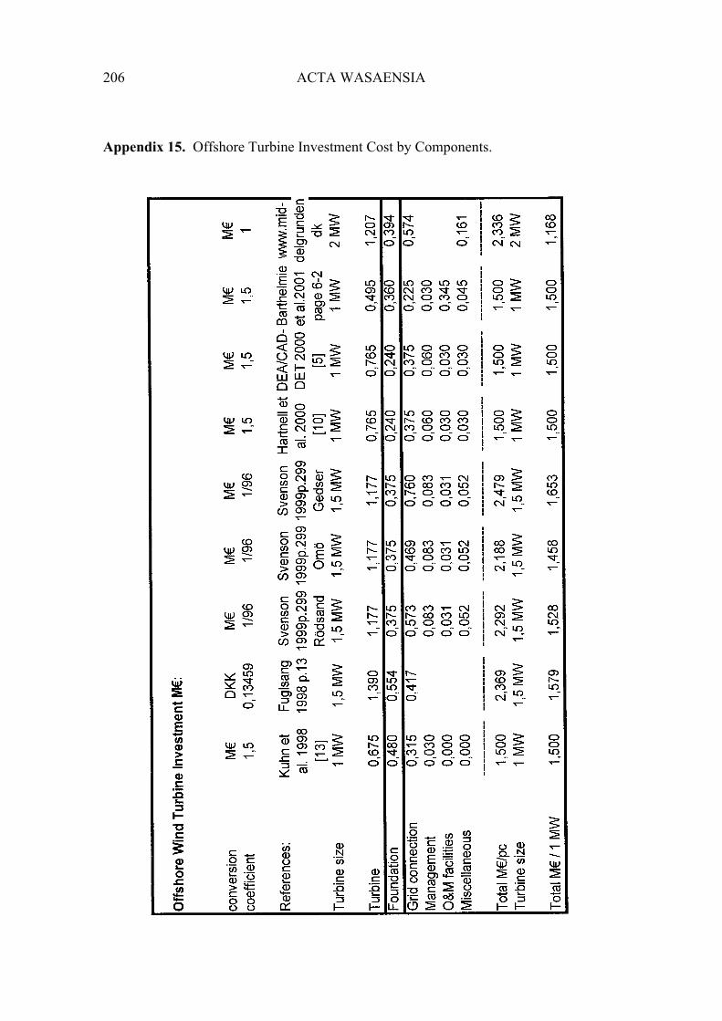
206 ACTA WASAENSIA

Appendix 15. Offshore Turbine Investment Cost by Components.

ACTA WASAENSIA 207

Appendix 16. Measuring Arrangements in Larsmo Region.

208 ACTA WASAENSIA

Appendix 17. Tankar and Fränsvik Wind Speed Differences by Wind Speeds and Wind

Direction Sectors.

ACTA WASAENSIA 209

210 ACTA WASAENSIA

ACTA WASAENSIA 211

Appendix 18. Offshore Market Plans for Years 2003 - 2010

Source: Own reseach, BTM Consult A/S-March 2001, New Energy 2001-2, Concerted

Action on Offshore Wind Energy in Europe 2001.

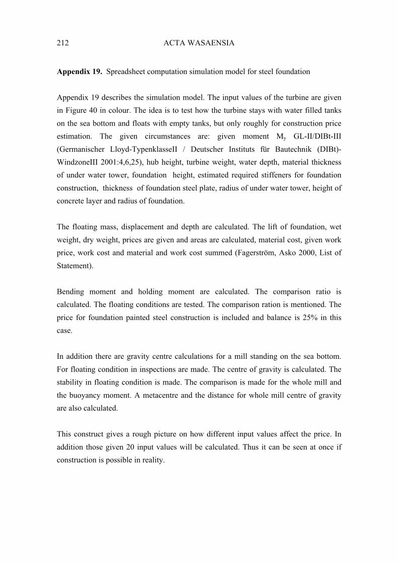
212 ACTA WASAENSIA

Appendix 19. Spreadsheet computation simulation model for steel foundation

Appendix 19 describes the simulation model. The input values of the turbine are given

in Figure 40 in colour. The idea is to test how the turbine stays with water filled tanks

on the sea bottom and floats with empty tanks, but only roughly for construction price

estimation. The given circumstances are: given moment My GL-II/DIBt-III

(Germanischer Lloyd-TypenklasseII / Deutscher Instituts für Bautechnik (DIBt)-

WindzoneIII 2001:4,6,25), hub height, turbine weight, water depth, material thickness

of under water tower, foundation height, estimated required stiffeners for foundation

construction, thickness of foundation steel plate, radius of under water tower, height of

concrete layer and radius of foundation.

The floating mass, displacement and depth are calculated. The lift of foundation, wet

weight, dry weight, prices are given and areas are calculated, material cost, given work

price, work cost and material and work cost summed (Fagerström, Asko 2000, List of

Statement).

Bending moment and holding moment are calculated. The comparison ratio is

calculated. The floating conditions are tested. The comparison ration is mentioned. The

price for foundation painted steel construction is included and balance is 25% in this

case.

In addition there are gravity centre calculations for a mill standing on the sea bottom.

For floating condition in inspections are made. The centre of gravity is calculated. The

stability in floating condition is made. The comparison is made for the whole mill and

the buoyancy moment. A metacentre and the distance for whole mill centre of gravity

are also calculated.

This construct gives a rough picture on how different input values affect the price. In

addition those given 20 input values will be calculated. Thus it can be seen at once if

construction is possible in reality.

Documents

YRJÖ RINTA-JOUPPI - Vaasan yliopisto · YRJÖ RINTA-JOUPPI Development of Offshore Wind Power Price Competitiveness Using a New Logistics Construct ... A/S, NORDEX A/S and Vestas