Introduction to Einstein’s Theoryof Relativity

Øyvind Grøn

From Newton’s Attractive Gravityto the Repulsive Gravity of VacuumEnergy

Second Edition

Undergraduate Texts in Physics

Undergraduate Texts in Physics

Series Editors

Kurt H. Becker, NYU Polytechnic School of Engineering, Brooklyn, NY, USA

Jean-Marc Di Meglio, Matière et Systèmes Complexes, Université Paris Diderot,Bâtiment Condorcet, Paris, France

Sadri D. Hassani, Department of Physics, Loomis Laboratory, University of Illinoisat Urbana-Champaign, Urbana, IL, USA

Morten Hjorth-Jensen, Department of Physics, Blindern, University of Oslo,Oslo, Norway

Michael Inglis, Patchogue, NY, USA

Bill Munro, NTT Basic Research Laboratories, Optical Science Laboratories,Atsugi, Kanagawa, Japan

Susan Scott, Department of Quantum Science, Australian National University,Acton, ACT, Australia

Martin Stutzmann, Walter Schottky Institute, Technical University of Munich,Garching, Bayern, Germany

Undergraduate Texts in Physics (UTP) publishes authoritative texts covering topicsencountered in a physics undergraduate syllabus. Each title in the series is suitableas an adopted text for undergraduate courses, typically containing practiceproblems, worked examples, chapter summaries, and suggestions for furtherreading. UTP titles should provide an exceptionally clear and concise treatment of asubject at undergraduate level, usually based on a successful lecture course. Coreand elective subjects are considered for inclusion in UTP.

UTP books will be ideal candidates for course adoption, providing lecturers witha firm basis for development of lecture series, and students with an essentialreference for their studies and beyond.

More information about this series at http://www.springer.com/series/15593

Øyvind Grøn

Introduction to Einstein’sTheory of RelativityFrom Newton’s Attractive Gravityto the Repulsive Gravity of Vacuum Energy

Second Edition

123

Øyvind GrønOsloMet—Oslo Metropolitan UniversityOslo, Norway

ISSN 2510-411X ISSN 2510-4128 (electronic)Undergraduate Texts in PhysicsISBN 978-3-030-43861-6 ISBN 978-3-030-43862-3 (eBook)https://doi.org/10.1007/978-3-030-43862-3

1st edition: © Springer Science+Business Media, LLC 20092nd edition: © Springer Nature Switzerland AG 2020This work is subject to copyright. All rights are reserved by the Publisher, whether the whole or partof the material is concerned, specifically the rights of translation, reprinting, reuse of illustrations,recitation, broadcasting, reproduction on microfilms or in any other physical way, and transmissionor information storage and retrieval, electronic adaptation, computer software, or by similar or dissimilarmethodology now known or hereafter developed.The use of general descriptive names, registered names, trademarks, service marks, etc. in thispublication does not imply, even in the absence of a specific statement, that such names are exempt fromthe relevant protective laws and regulations and therefore free for general use.The publisher, the authors and the editors are safe to assume that the advice and information in thisbook are believed to be true and accurate at the date of publication. Neither the publisher nor theauthors or the editors give a warranty, expressed or implied, with respect to the material containedherein or for any errors or omissions that may have been made. The publisher remains neutral with regardto jurisdictional claims in published maps and institutional affiliations.

This Springer imprint is published by the registered company Springer Nature Switzerland AGThe registered company address is: Gewerbestrasse 11, 6330 Cham, Switzerland

Preface to the Second Edition

These notes are a transcript of lectures delivered by Øyvind Grøn during the springof 1997 at the University of Oslo. The manuscript has been revised in 2019. Thepresent version of this document is an extended and corrected version of a set ofLecture Notes which were written down by S. Bard, Andreas O. Jaunsen, FrodeHansen and Ragnvald J. Irgens using LATEX2�. Sven E. Hjelmeland has mademany useful suggestions which have improved the text.

The manuscript has been revised in 2019. In this version, solutions to theexercises have been included. Most of these have been provided by Håkon Enger.I thank all my good helpers for enthusiastic work which was decisive for therealization of the book.

I hope that these notes are useful to students of general relativity and lookforward to their comments accepting all feedback with thanks. The comments maybe sent to the author by e-mail to oyvind.gron.no@gmail.com.

Oslo, Norway Øyvind Grøn

v

Preface to the First Edition

These notes are a transcript of lectures delivered by Øyvind Grøn during the springof 1997 at the University of Oslo.

The present version of this document is an extended and corrected version of aset of Lecture Notes which were typesetted by S. Bard, Andreas O. Jaunsen, FrodeHansen and Ragnvald J. Irgens using LATEX2�. Svend E. Hjelmeland has mademany useful suggestions which have improved the text. I would also like to thankJon Magne Leinaas and Sigbjørn Hervik for contributing with problems and GormKrogh Johnsen for help with finishing the manuscript. I also want to thank Prof.Finn Ravndal for inspiring lectures on general relativity.

While we hope that these typeset notes are of benefit particularly to students ofgeneral relativity and look forward to their comments, we welcome all interestedreaders and accept all feedback with thanks.

All comments may be sent to the author by e-mail.

E-mail: Oyvind.Gron@iu.hio.no Øyvind Grøn

vii

Contents

1 Newton’s Theory of Gravitation . . . . . . . . . . . . . . . . . . . . . . . . . . . 11.1 The Force Law of Gravitation . . . . . . . . . . . . . . . . . . . . . . . . . 21.2 Newton’s Law of Gravitation in Local Form . . . . . . . . . . . . . . 41.3 Newtonian Incompressible Star . . . . . . . . . . . . . . . . . . . . . . . . 71.4 Tidal Forces . . . . . . . . . . . . . . . . . . . . . . . . . . . . . . . . . . . . . . 101.5 The Principle of Equivalence . . . . . . . . . . . . . . . . . . . . . . . . . . 141.6 The General Principle of Relativity . . . . . . . . . . . . . . . . . . . . . 171.7 The Covariance Principle . . . . . . . . . . . . . . . . . . . . . . . . . . . . 171.8 Mach’s Principle . . . . . . . . . . . . . . . . . . . . . . . . . . . . . . . . . . . 181.9 Exercises . . . . . . . . . . . . . . . . . . . . . . . . . . . . . . . . . . . . . . . . 19References . . . . . . . . . . . . . . . . . . . . . . . . . . . . . . . . . . . . . . . . . . . . 22

2 The Special Theory of Relativity . . . . . . . . . . . . . . . . . . . . . . . . . . . 232.1 Coordinate Systems and Minkowski Diagrams . . . . . . . . . . . . . 232.2 Synchronization of Clocks . . . . . . . . . . . . . . . . . . . . . . . . . . . . 252.3 The Doppler Effect . . . . . . . . . . . . . . . . . . . . . . . . . . . . . . . . . 262.4 Relativistic Time Dilation . . . . . . . . . . . . . . . . . . . . . . . . . . . . 282.5 The Relativity of Simultaneity . . . . . . . . . . . . . . . . . . . . . . . . . 302.6 The Lorentz Contraction . . . . . . . . . . . . . . . . . . . . . . . . . . . . . 332.7 The Lorentz Transformation . . . . . . . . . . . . . . . . . . . . . . . . . . 342.8 Lorentz Invariant Interval . . . . . . . . . . . . . . . . . . . . . . . . . . . . 372.9 The Twin Paradox . . . . . . . . . . . . . . . . . . . . . . . . . . . . . . . . . 402.10 Hyperbolic Motion . . . . . . . . . . . . . . . . . . . . . . . . . . . . . . . . . 412.11 Energy and Mass . . . . . . . . . . . . . . . . . . . . . . . . . . . . . . . . . . 442.12 Relativistic Increase of Mass . . . . . . . . . . . . . . . . . . . . . . . . . . 452.13 Lorentz Transformation of Velocity, Momentum,

Energy and Force . . . . . . . . . . . . . . . . . . . . . . . . . . . . . . . . . . 472.14 Tachyons . . . . . . . . . . . . . . . . . . . . . . . . . . . . . . . . . . . . . . . . 502.15 Magnetism as a Relativistic Second-Order Effect . . . . . . . . . . . 51

ix

Exercises . . . . . . . . . . . . . . . . . . . . . . . . . . . . . . . . . . . . . . . . . . . . . 54Reference . . . . . . . . . . . . . . . . . . . . . . . . . . . . . . . . . . . . . . . . . . . . . 58

3 Vectors, Tensors and Forms . . . . . . . . . . . . . . . . . . . . . . . . . . . . . . 593.1 Vectors . . . . . . . . . . . . . . . . . . . . . . . . . . . . . . . . . . . . . . . . . 59

3.1.1 Four-Vectors . . . . . . . . . . . . . . . . . . . . . . . . . . . . . . . 603.1.2 Tangent Vector Fields and Coordinate Vectors . . . . . . . 623.1.3 Coordinate Transformations . . . . . . . . . . . . . . . . . . . . 653.1.4 Structure Coefficients . . . . . . . . . . . . . . . . . . . . . . . . . 68

3.2 Tensors . . . . . . . . . . . . . . . . . . . . . . . . . . . . . . . . . . . . . . . . . 693.2.1 Transformation of Tensor Components . . . . . . . . . . . . 713.2.2 Transformation of Basis One-Forms . . . . . . . . . . . . . . 713.2.3 The Metric Tensor . . . . . . . . . . . . . . . . . . . . . . . . . . . 72

3.3 The Causal Structure of Spacetime . . . . . . . . . . . . . . . . . . . . . . 763.4 Forms . . . . . . . . . . . . . . . . . . . . . . . . . . . . . . . . . . . . . . . . . . 78

3.4.1 The Volume Form . . . . . . . . . . . . . . . . . . . . . . . . . . . 803.4.2 Dual Forms . . . . . . . . . . . . . . . . . . . . . . . . . . . . . . . . 82

Exercises . . . . . . . . . . . . . . . . . . . . . . . . . . . . . . . . . . . . . . . . . . . . . 85

4 Accelerated Reference Frames . . . . . . . . . . . . . . . . . . . . . . . . . . . . 894.1 The Spatial Metric Tensor . . . . . . . . . . . . . . . . . . . . . . . . . . . . 894.2 Einstein Synchronization of Clocks in a Rotating

Reference Frame . . . . . . . . . . . . . . . . . . . . . . . . . . . . . . . . . . . 924.3 Angular Acceleration in the Rotating Frame . . . . . . . . . . . . . . . 954.4 Gravitational Time Dilation . . . . . . . . . . . . . . . . . . . . . . . . . . . 984.5 Path of Photons Emitted from the Axis in a Rotating

Reference Frame . . . . . . . . . . . . . . . . . . . . . . . . . . . . . . . . . . . 994.6 The Sagnac Effect . . . . . . . . . . . . . . . . . . . . . . . . . . . . . . . . . . 994.7 Non-integrability of a Simultaneity Curve in a Rotating

Frame . . . . . . . . . . . . . . . . . . . . . . . . . . . . . . . . . . . . . . . . . . 1014.8 Orthonormal Basis Field in a Rotating Frame . . . . . . . . . . . . . . 1024.9 Uniformly Accelerated Reference Frame . . . . . . . . . . . . . . . . . 1054.10 The Projection Tensor . . . . . . . . . . . . . . . . . . . . . . . . . . . . . . . 113Exercises . . . . . . . . . . . . . . . . . . . . . . . . . . . . . . . . . . . . . . . . . . . . . 115

5 Covariant Differentiation . . . . . . . . . . . . . . . . . . . . . . . . . . . . . . . . 1195.1 Differentiation of Forms . . . . . . . . . . . . . . . . . . . . . . . . . . . . . 119

5.1.1 Exterior Differentiation . . . . . . . . . . . . . . . . . . . . . . . . 1195.1.2 Covariant Derivative . . . . . . . . . . . . . . . . . . . . . . . . . . 122

5.2 The Christoffel Symbols . . . . . . . . . . . . . . . . . . . . . . . . . . . . . 1225.3 Geodesic Curves . . . . . . . . . . . . . . . . . . . . . . . . . . . . . . . . . . . 1255.4 The Covariant Euler–Lagrange Equations . . . . . . . . . . . . . . . . . 1275.5 Application of the Lagrange Formalism to Free Particles . . . . . . 129

5.5.1 Equation of Motion from Lagrange’s Equations . . . . . . 1295.5.2 Geodesic World Lines in Spacetime . . . . . . . . . . . . . . 133

x Contents

5.5.3 Acceleration of Gravity . . . . . . . . . . . . . . . . . . . . . . . . 1355.5.4 Gravitational Shift of Wavelength . . . . . . . . . . . . . . . . 138

5.6 Connection Coefficients . . . . . . . . . . . . . . . . . . . . . . . . . . . . . . 1405.6.1 Structure Coefficients . . . . . . . . . . . . . . . . . . . . . . . . . 143

5.7 Covariant Differentiation of Vectors, Forms and Tensors . . . . . . 1445.7.1 Covariant Differentiation of Vectors . . . . . . . . . . . . . . 1445.7.2 Covariant Differentiation of Forms . . . . . . . . . . . . . . . 1455.7.3 Covariant Differentiation of Tensors of Arbitrary

Rank . . . . . . . . . . . . . . . . . . . . . . . . . . . . . . . . . . . . . 1465.8 The Cartan Connection . . . . . . . . . . . . . . . . . . . . . . . . . . . . . . 1475.9 Covariant Decomposition of a Velocity Field . . . . . . . . . . . . . . 151

5.9.1 Newtonian 3-Velocity . . . . . . . . . . . . . . . . . . . . . . . . . 1515.9.2 Relativistic 4-Velocity . . . . . . . . . . . . . . . . . . . . . . . . 153

5.10 Killing Vectors and Symmetries . . . . . . . . . . . . . . . . . . . . . . . 1555.11 Covariant Expressions for Gradient, Divergence, Curl,

Laplacian and D’Alembert’s Wave Operator . . . . . . . . . . . . . . . 1575.12 Electromagnetism in Form Language . . . . . . . . . . . . . . . . . . . . 163Exercises . . . . . . . . . . . . . . . . . . . . . . . . . . . . . . . . . . . . . . . . . . . . . 169

6 Curvature . . . . . . . . . . . . . . . . . . . . . . . . . . . . . . . . . . . . . . . . . . . . 1736.1 The Riemann Curvature Tensor . . . . . . . . . . . . . . . . . . . . . . . . 1736.2 Differential Geometry of Surfaces . . . . . . . . . . . . . . . . . . . . . . 179

6.2.1 Surface Curvature Using the Cartan Formalism . . . . . . 1836.3 The Ricci Identity . . . . . . . . . . . . . . . . . . . . . . . . . . . . . . . . . . 1846.4 Bianchi’s 1. Identity . . . . . . . . . . . . . . . . . . . . . . . . . . . . . . . . 1856.5 Bianchi’s 2. Identity . . . . . . . . . . . . . . . . . . . . . . . . . . . . . . . . 1866.6 Torsion . . . . . . . . . . . . . . . . . . . . . . . . . . . . . . . . . . . . . . . . . 1876.7 The Equation of Geodesic Deviation . . . . . . . . . . . . . . . . . . . . 1886.8 Tidal Acceleration and Spacetime Curvature . . . . . . . . . . . . . . . 1906.9 The Newtonian Tidal Tensor . . . . . . . . . . . . . . . . . . . . . . . . . . 1916.10 The Tidal and Non-tidal Components of a Gravitational

Field . . . . . . . . . . . . . . . . . . . . . . . . . . . . . . . . . . . . . . . . . . . 192Exercises . . . . . . . . . . . . . . . . . . . . . . . . . . . . . . . . . . . . . . . . . . . . . 195

7 Einstein’s Field Equations . . . . . . . . . . . . . . . . . . . . . . . . . . . . . . . . 1977.1 Newtonian Fluid . . . . . . . . . . . . . . . . . . . . . . . . . . . . . . . . . . . 1977.2 Perfect Fluids . . . . . . . . . . . . . . . . . . . . . . . . . . . . . . . . . . . . . 199

7.2.1 Lorentz Invariant Vacuum Energy—LIVE . . . . . . . . . . 2007.2.2 Energy–Momentum Tensor of an Electromagnetic

Field . . . . . . . . . . . . . . . . . . . . . . . . . . . . . . . . . . . . . 2017.3 Einstein’s Curvature Tensor . . . . . . . . . . . . . . . . . . . . . . . . . . . 2017.4 Einstein’s Field Equations . . . . . . . . . . . . . . . . . . . . . . . . . . . . 2027.5 The “Geodesic Postulate” as a Consequence of the Field

Equations . . . . . . . . . . . . . . . . . . . . . . . . . . . . . . . . . . . . . . . . 204

Contents xi

7.6 Einstein’s Field Equations Deduced from a VariationalPrinciple . . . . . . . . . . . . . . . . . . . . . . . . . . . . . . . . . . . . . . . . . 206

Exercises . . . . . . . . . . . . . . . . . . . . . . . . . . . . . . . . . . . . . . . . . . . . . 210

8 Schwarzschild Spacetime . . . . . . . . . . . . . . . . . . . . . . . . . . . . . . . . . 2118.1 Schwarzschild’s Exterior Solution . . . . . . . . . . . . . . . . . . . . . . 2118.2 Radial Free Fall in Schwarzschild Spacetime . . . . . . . . . . . . . . 2178.3 Light Cones in Schwarzschild Spacetime . . . . . . . . . . . . . . . . . 2188.4 Analytical Extension of the Curvature Coordinates . . . . . . . . . . 2228.5 Embedding of the Schwarzschild Metric . . . . . . . . . . . . . . . . . . 2258.6 The Shapiro Experiment . . . . . . . . . . . . . . . . . . . . . . . . . . . . . 2268.7 Particle Trajectories in Schwarzschild 3-Space . . . . . . . . . . . . . 228

8.7.1 Motion in the Equatorial Plane . . . . . . . . . . . . . . . . . . 2298.8 Classical Tests of Einstein’s General Theory of Relativity . . . . . 232

8.8.1 The Hafele–Keating Experiment . . . . . . . . . . . . . . . . . 2328.8.2 Mercury’s Perihelion Precession . . . . . . . . . . . . . . . . . 2338.8.3 Deflection of Light . . . . . . . . . . . . . . . . . . . . . . . . . . . 236

8.9 The Reissner–Nordström Spacetime . . . . . . . . . . . . . . . . . . . . . 238Exercises . . . . . . . . . . . . . . . . . . . . . . . . . . . . . . . . . . . . . . . . . . . . . 240References . . . . . . . . . . . . . . . . . . . . . . . . . . . . . . . . . . . . . . . . . . . . 242

9 The Linear Field Approximation and Gravitational Waves . . . . . . 2439.1 The Linear Field Approximation . . . . . . . . . . . . . . . . . . . . . . . 2439.2 Solutions of the Linearized Field Equations . . . . . . . . . . . . . . . 246

9.2.1 The Gravitational Potential of a Point Mass . . . . . . . . . 2469.2.2 Spacetime Inside and Outside a Rotating Spherical

Shell . . . . . . . . . . . . . . . . . . . . . . . . . . . . . . . . . . . . . 2479.3 Inertial Dragging . . . . . . . . . . . . . . . . . . . . . . . . . . . . . . . . . . . 2509.4 Gravitoelectromagnetism . . . . . . . . . . . . . . . . . . . . . . . . . . . . . 2519.5 Gravitational Waves . . . . . . . . . . . . . . . . . . . . . . . . . . . . . . . . 253

9.5.1 What Sort of Gravitational Waves Is Predictedby Einstein’s Theory? . . . . . . . . . . . . . . . . . . . . . . . . . 255

9.5.2 Polarization of the Gravitational Waves . . . . . . . . . . . . 2569.6 The Effect of Gravitational Waves upon Matter . . . . . . . . . . . . 2579.7 The LIGO-Detection of Gravitational Waves . . . . . . . . . . . . . . 260

9.7.1 Kepler’s Third Law and the Strainof the Detector . . . . . . . . . . . . . . . . . . . . . . . . . . . . . . 262

9.7.2 Newtonian Description of a Binary System . . . . . . . . . 2659.7.3 Gravitational Radiation Emission . . . . . . . . . . . . . . . . . 2669.7.4 The Chirp . . . . . . . . . . . . . . . . . . . . . . . . . . . . . . . . . 267

References . . . . . . . . . . . . . . . . . . . . . . . . . . . . . . . . . . . . . . . . . . . . 269

xii Contents

10 Black Holes . . . . . . . . . . . . . . . . . . . . . . . . . . . . . . . . . . . . . . . . . . . 27110.1 “Surface Gravity”: Acceleration of Gravity

at the Horizon of a Black Hole . . . . . . . . . . . . . . . . . . . . . . . . 27110.2 Hawking Radiation: Radiation from a Black Hole . . . . . . . . . . . 27310.3 Rotating Black Holes: The Kerr Metric . . . . . . . . . . . . . . . . . . 275

10.3.1 Zero-Angular Momentum Observers . . . . . . . . . . . . . . 27610.3.2 Does the Kerr Spacetime Have a Horizon? . . . . . . . . . 277

Exercises . . . . . . . . . . . . . . . . . . . . . . . . . . . . . . . . . . . . . . . . . . . . . 279

11 Sources of Gravitational Fields . . . . . . . . . . . . . . . . . . . . . . . . . . . . 28311.1 The Pressure Contribution to the Gravitational Mass

of a Static, Spherically Symmetric System . . . . . . . . . . . . . . . . 28311.2 The Tolman–Oppenheimer–Volkoff Equation . . . . . . . . . . . . . . 28511.3 An Exact Solution for Incompressible Stars—Schwarzschild’s

Interior Solution . . . . . . . . . . . . . . . . . . . . . . . . . . . . . . . . . . . 28711.4 The Israel Formalism for Describing Singular Mass Shells

in the General Theory of Relativity . . . . . . . . . . . . . . . . . . . . . 29011.5 The Levi-Civita—Bertotti—Robinson Solution of Einstein’s

Field Equations . . . . . . . . . . . . . . . . . . . . . . . . . . . . . . . . . . . . 29511.6 The Source of the Levi-Civita—Bertotti—Robinson

Spacetime . . . . . . . . . . . . . . . . . . . . . . . . . . . . . . . . . . . . . . . . 29711.7 A Source of the Kerr–Newman Spacetime . . . . . . . . . . . . . . . . 29911.8 Physical Interpretation of the Components

of the Energy–Momentum Tensor by Meansof the Eigenvalues of the Tensor . . . . . . . . . . . . . . . . . . . . . . . 302

11.9 The River of Space . . . . . . . . . . . . . . . . . . . . . . . . . . . . . . . . . 305Exercises . . . . . . . . . . . . . . . . . . . . . . . . . . . . . . . . . . . . . . . . . . . . . 309References . . . . . . . . . . . . . . . . . . . . . . . . . . . . . . . . . . . . . . . . . . . . 309

12 Cosmology . . . . . . . . . . . . . . . . . . . . . . . . . . . . . . . . . . . . . . . . . . . . 31112.1 Co-moving Coordinate System . . . . . . . . . . . . . . . . . . . . . . . . 31112.2 Curvature Isotropy—The Robertson–Walker Metric . . . . . . . . . 31212.3 Cosmic Kinematics and Dynamics . . . . . . . . . . . . . . . . . . . . . . 314

12.3.1 The Hubble–Lemaître Law . . . . . . . . . . . . . . . . . . . . . 31412.3.2 Cosmological Redshift of Light . . . . . . . . . . . . . . . . . . 31512.3.3 Cosmic Fluids . . . . . . . . . . . . . . . . . . . . . . . . . . . . . . 31712.3.4 Isotropic and Homogeneous Universe Models . . . . . . . 31812.3.5 Cosmic Redshift . . . . . . . . . . . . . . . . . . . . . . . . . . . . . 32312.3.6 Energy–Momentum Conservation . . . . . . . . . . . . . . . . 326

12.4 Some LFRW Cosmological Models . . . . . . . . . . . . . . . . . . . . . 33012.4.1 Radiation-Dominated Universe Model . . . . . . . . . . . . . 33012.4.2 Dust-Dominated Universe Model . . . . . . . . . . . . . . . . 33112.4.3 Transition from Radiation-Dominated

to Matter-Dominated Universe . . . . . . . . . . . . . . . . . . 335

Contents xiii

12.4.4 The de Sitter Universe Models . . . . . . . . . . . . . . . . . . 33612.4.5 The Friedmann–Lemaître Model . . . . . . . . . . . . . . . . . 33712.4.6 Flat Universe with Dust and Phantom Energy . . . . . . . 348

12.5 Flat Anisotropic Universe Models . . . . . . . . . . . . . . . . . . . . . . 35112.6 Inhomogeneous Universe Models . . . . . . . . . . . . . . . . . . . . . . . 355

12.6.1 Dust-Dominated Model . . . . . . . . . . . . . . . . . . . . . . . . 35612.6.2 Inhomogeneous Universe Model with Dust

and LIVE . . . . . . . . . . . . . . . . . . . . . . . . . . . . . . . . . 35712.7 The Horizon and Flatness Problems . . . . . . . . . . . . . . . . . . . . . 358

12.7.1 The Horizon Problem . . . . . . . . . . . . . . . . . . . . . . . . . 35812.7.2 The Flatness Problem . . . . . . . . . . . . . . . . . . . . . . . . . 360

12.8 Inflationary Universe Models . . . . . . . . . . . . . . . . . . . . . . . . . . 36112.8.1 Spontaneous Symmetry Breaking and the Higgs

Mechanism . . . . . . . . . . . . . . . . . . . . . . . . . . . . . . . . 36112.8.2 Guth’s Inflationary Model . . . . . . . . . . . . . . . . . . . . . . 36312.8.3 The Inflationary Models’ Answers to the Problems

of the Friedmann Models . . . . . . . . . . . . . . . . . . . . . . 36412.8.4 Dynamics of the Inflationary Era . . . . . . . . . . . . . . . . . 36612.8.5 Testing Observable Consequences of the Inflationary

Era . . . . . . . . . . . . . . . . . . . . . . . . . . . . . . . . . . . . . . 37212.9 The Significance of Inertial Dragging for the Relativity

of Rotation . . . . . . . . . . . . . . . . . . . . . . . . . . . . . . . . . . . . . . . 37712.9.1 The Cosmic Causal Mass in the Einstein-de Sitter

Universe . . . . . . . . . . . . . . . . . . . . . . . . . . . . . . . . . . 37812.9.2 The Cosmic Causal Mass in the Flat KCDM

Universe . . . . . . . . . . . . . . . . . . . . . . . . . . . . . . . . . . 380Exercises . . . . . . . . . . . . . . . . . . . . . . . . . . . . . . . . . . . . . . . . . . . . . 382References . . . . . . . . . . . . . . . . . . . . . . . . . . . . . . . . . . . . . . . . . . . . 390

Appendix: Kaluza–Klein Theory . . . . . . . . . . . . . . . . . . . . . . . . . . . . . . . . 393

Solutions to the Exercises . . . . . . . . . . . . . . . . . . . . . . . . . . . . . . . . . . . . . . 409

Index . . . . . . . . . . . . . . . . . . . . . . . . . . . . . . . . . . . . . . . . . . . . . . . . . . . . . . 511

xiv Contents

List of Figures

Fig. 1.1 Newton’s law of gravitation . . . . . . . . . . . . . . . . . . . . . . . . . . . 2Fig. 1.2 Deduction of Newton’s law of gravitation in local form. . . . . . 4Fig. 1.3 Solid angle . . . . . . . . . . . . . . . . . . . . . . . . . . . . . . . . . . . . . . . . 6Fig. 1.4 Mass shell in a star . . . . . . . . . . . . . . . . . . . . . . . . . . . . . . . . . . 9Fig. 1.5 Tidal forces. . . . . . . . . . . . . . . . . . . . . . . . . . . . . . . . . . . . . . . . 10Fig. 1.6 Horizontal tidal force . . . . . . . . . . . . . . . . . . . . . . . . . . . . . . . . 11Fig. 1.7 An elastic ring originally circular, falling freely

in the gravitational field of the Earth . . . . . . . . . . . . . . . . . . . . 12Fig. 1.8 The Earth–Moon system . . . . . . . . . . . . . . . . . . . . . . . . . . . . . . 13Fig. 1.9 Tidal acceleration field . . . . . . . . . . . . . . . . . . . . . . . . . . . . . . . 14Fig. 1.10 A tidal force pendulum . . . . . . . . . . . . . . . . . . . . . . . . . . . . . . . 20Fig. 2.1 World lines . . . . . . . . . . . . . . . . . . . . . . . . . . . . . . . . . . . . . . . . 25Fig. 2.2 Clock synchronization by the radar method . . . . . . . . . . . . . . . 26Fig. 2.3 The Doppler effect . . . . . . . . . . . . . . . . . . . . . . . . . . . . . . . . . . 27Fig. 2.4 Photon clock at rest . . . . . . . . . . . . . . . . . . . . . . . . . . . . . . . . . 29Fig. 2.5 Moving photon clock . . . . . . . . . . . . . . . . . . . . . . . . . . . . . . . . 29Fig. 2.6 Simultaneous events . . . . . . . . . . . . . . . . . . . . . . . . . . . . . . . . . 31Fig. 2.7 The simultaneous events of Fig. 2.6 in another frame. . . . . . . . 31Fig. 2.8 Light flash in a moving train . . . . . . . . . . . . . . . . . . . . . . . . . . 32Fig. 2.9 Length contraction . . . . . . . . . . . . . . . . . . . . . . . . . . . . . . . . . . 33Fig. 2.10 Space-like, light-like and time-like intervals . . . . . . . . . . . . . . . 38Fig. 2.11 World line of an accelerating particle . . . . . . . . . . . . . . . . . . . . 39Fig. 2.12 Twin paradox world lines . . . . . . . . . . . . . . . . . . . . . . . . . . . . . 40Fig. 2.13 World line of particle with constant rest acceleration . . . . . . . . 43Fig. 2.14 Light pulse in a box . . . . . . . . . . . . . . . . . . . . . . . . . . . . . . . . . 44Fig. 2.15 Tachyon paradox . . . . . . . . . . . . . . . . . . . . . . . . . . . . . . . . . . . 51Fig. 2.16 Current carrying wire seen from its own rest frame . . . . . . . . . 52Fig. 2.17 Current carrying wire seen from the frame of a moving

charge . . . . . . . . . . . . . . . . . . . . . . . . . . . . . . . . . . . . . . . . . . . . 53Fig. 2.18 Light cone due to Cherenkov radiation . . . . . . . . . . . . . . . . . . . 55Fig. 3.1 Closed polygon (linearly dependent vectors). . . . . . . . . . . . . . . 60

xv

Fig. 3.2 No finite position vector in curved space . . . . . . . . . . . . . . . . . 63Fig. 3.3 Vectors in tangent planes . . . . . . . . . . . . . . . . . . . . . . . . . . . . . 63Fig. 3.4 Basis vectors in Cartesian- and plane polar coordinates . . . . . . 67Fig. 3.5 Basis vectors in a skew angled coordinate system . . . . . . . . . . 73Fig. 3.6 Covariant and contravariant components of a vector. . . . . . . . . 75Fig. 3.7 Causal structure of spacetime . . . . . . . . . . . . . . . . . . . . . . . . . . 77Fig. 4.1 Simultaneity in a rotating frame . . . . . . . . . . . . . . . . . . . . . . . . 92Fig. 4.2 Discontinuity of simultaneity in rotating frame . . . . . . . . . . . . . 93Fig. 4.3 Nonrotating disc with measuring rods. . . . . . . . . . . . . . . . . . . . 96Fig. 4.4 Lorentz contacted measuring rods on a rotating disc. . . . . . . . . 97Fig. 4.5 The Sagnac effect . . . . . . . . . . . . . . . . . . . . . . . . . . . . . . . . . . . 100Fig. 4.6 Discontinuous simultaneity surface in a rotating frame . . . . . . . 102Fig. 4.7 Rigid rotation . . . . . . . . . . . . . . . . . . . . . . . . . . . . . . . . . . . . . . 104Fig. 4.8 Hyperbolic motion . . . . . . . . . . . . . . . . . . . . . . . . . . . . . . . . . . 106Fig. 4.9 The velocity of a uniformly accelerated particle . . . . . . . . . . . . 108Fig. 4.10 Simultaneity in a uniformly accelerated reference frame . . . . . . 109Fig. 4.11 World lines and simultaneity lines of a uniformly

accelerated reference system . . . . . . . . . . . . . . . . . . . . . . . . . . . 111Fig. 5.1 Parallel transport . . . . . . . . . . . . . . . . . . . . . . . . . . . . . . . . . . . . 125Fig. 5.2 Geodesic curve on a flat surface . . . . . . . . . . . . . . . . . . . . . . . . 126Fig. 5.3 Geodesic curves on a sphere . . . . . . . . . . . . . . . . . . . . . . . . . . . 126Fig. 5.4 Neighboring geodesics in a Minkowski diagram. . . . . . . . . . . . 127Fig. 5.5 Time like geodesics . . . . . . . . . . . . . . . . . . . . . . . . . . . . . . . . . 133Fig. 5.6 Projectiles in 3-space . . . . . . . . . . . . . . . . . . . . . . . . . . . . . . . . 134Fig. 5.7 The twin paradox . . . . . . . . . . . . . . . . . . . . . . . . . . . . . . . . . . . 136Fig. 5.8 Rotating coordinate system . . . . . . . . . . . . . . . . . . . . . . . . . . . . 141Fig. 6.1 Parallel transport . . . . . . . . . . . . . . . . . . . . . . . . . . . . . . . . . . . . 174Fig. 6.2 Parallel transport of a vector around a triangle . . . . . . . . . . . . . 174Fig. 6.3 Curvature and parallel transport . . . . . . . . . . . . . . . . . . . . . . . . 175Fig. 6.4 Curl as area of a vectorial parallelogram. . . . . . . . . . . . . . . . . . 176Fig. 6.5 Surface with tangent vectors and normal vector . . . . . . . . . . . . 180Fig. 6.6 Geodesic deviation . . . . . . . . . . . . . . . . . . . . . . . . . . . . . . . . . . 189Fig. 6.7 Spacetime curvature and the tidal force pendulum . . . . . . . . . . 196Fig. 8.1 Light cones in Schwarzschild spacetime with Schwarzschild

time. . . . . . . . . . . . . . . . . . . . . . . . . . . . . . . . . . . . . . . . . . . . . . 220Fig. 8.2 Light cones in Schwarzschild spacetime with

Eddington-Finkelstein time . . . . . . . . . . . . . . . . . . . . . . . . . . . . 221Fig. 8.3 Embedding of the extended Schwarzschild spacetime. . . . . . . . 226Fig. 8.4 The Shapiro experiment . . . . . . . . . . . . . . . . . . . . . . . . . . . . . . 227Fig. 8.5 Newtonian centrifugal barrier . . . . . . . . . . . . . . . . . . . . . . . . . . 230Fig. 8.6 Relativistic gravitational potential outside a spherical body . . . 231Fig. 8.7 Deflection of light . . . . . . . . . . . . . . . . . . . . . . . . . . . . . . . . . . . 237Fig. 9.1 Deformation of a ring of free particles caused by a

gravitational wave with + polarization . . . . . . . . . . . . . . . . . . . 259

xvi List of Figures

Fig. 9.2 Deformation of a ring of free particles causedby a gravitational wave with x polarization . . . . . . . . . . . . . . . 260

Fig. 9.3 LIGO gravitational wave detector . . . . . . . . . . . . . . . . . . . . . . . 261Fig. 9.4 LIGO-gravitational wave signal . . . . . . . . . . . . . . . . . . . . . . . . 262Fig. 9.5 LIGO gravitational wave discovery signal . . . . . . . . . . . . . . . . 263Fig. 10.1 Static border and horizon of a Kerr black . . . . . . . . . . . . . . . . . 279Fig. 11.1 River of space in the Schwarzschild-de Sitter spacetime. . . . . . 308Fig. 12.1 Cosmological redshift . . . . . . . . . . . . . . . . . . . . . . . . . . . . . . . . 316Fig. 12.2 Expansion of a radiation dominated universe . . . . . . . . . . . . . . 331Fig. 12.3 Expansion of matter dominated universe models . . . . . . . . . . . 334Fig. 12.4 Hubble age . . . . . . . . . . . . . . . . . . . . . . . . . . . . . . . . . . . . . . . . 334Fig. 12.5 The scale factor of the De Sitter universe models . . . . . . . . . . . 337Fig. 12.6 The scale factor of the flat KCDM universe model. . . . . . . . . . 340Fig. 12.7 The ratio of age and Hubble age of the flat KCDM

universe model . . . . . . . . . . . . . . . . . . . . . . . . . . . . . . . . . . . . . 340Fig. 12.8 Age-redshift relation of the flat KCDM universe model . . . . . . 341Fig. 12.9 The Hubble parameter of the flat KCDM universe model. . . . . 342Fig. 12.10 The deceleration parameter of the flat KCDM universe

model . . . . . . . . . . . . . . . . . . . . . . . . . . . . . . . . . . . . . . . . . . . . 343Fig. 12.11 Point of time for deceleration–acceleration turnover . . . . . . . . . 344Fig. 12.12 Cosmic redshift at the deceleration–acceleration turnover . . . . . 345Fig. 12.13 Critical density as function of time . . . . . . . . . . . . . . . . . . . . . . 345Fig. 12.14 The density parameter of vacuum energy as function

of time . . . . . . . . . . . . . . . . . . . . . . . . . . . . . . . . . . . . . . . . . . . 346Fig. 12.15 The density of matter as function of time . . . . . . . . . . . . . . . . . 347Fig. 12.16 The density parameter of matter as a function of time . . . . . . . 347Fig. 12.17 Evolution of anisotropy in a LIVE-dominated

Bianchi-type I universe . . . . . . . . . . . . . . . . . . . . . . . . . . . . . . . 355Fig. 12.18 Inflationary potentials . . . . . . . . . . . . . . . . . . . . . . . . . . . . . . . . 362Fig. 12.19 Temperature dependence of Higgs potential . . . . . . . . . . . . . . . 363Fig. 12.20 Polarization of electromagnetic radiation. . . . . . . . . . . . . . . . . . 372Fig. 12.21 Causal mass . . . . . . . . . . . . . . . . . . . . . . . . . . . . . . . . . . . . . . . 381

List of Figures xvii

List of Definitions

Definition 3.1.1 Four-velocity . . . . . . . . . . . . . . . . . . . . . . . . . . . . . . . . . 60Definition 3.1.2 Four-momentum . . . . . . . . . . . . . . . . . . . . . . . . . . . . . . . 61Definition 3.1.3 Minkowski force. . . . . . . . . . . . . . . . . . . . . . . . . . . . . . . 62Definition 3.1.4 Four-acceleration . . . . . . . . . . . . . . . . . . . . . . . . . . . . . . 62Definition 3.1.5 Reference frame . . . . . . . . . . . . . . . . . . . . . . . . . . . . . . . 64Definition 3.1.6 Coordinate system . . . . . . . . . . . . . . . . . . . . . . . . . . . . . 64Definition 3.1.7 Co-moving coordinate system. . . . . . . . . . . . . . . . . . . . . 64Definition 3.1.8 Orthonormal basis. . . . . . . . . . . . . . . . . . . . . . . . . . . . . . 64Definition 3.1.9 Preliminary definition of coordinate basis vector . . . . . . 64Definition 3.1.10 General definition of coordinate basis vectors. . . . . . . . . 66Definition 3.1.11 Orthonormal basis. . . . . . . . . . . . . . . . . . . . . . . . . . . . . . 67Definition 3.1.12 Commutator of vectors . . . . . . . . . . . . . . . . . . . . . . . . . . 68Definition 3.1.13 Structure coefficients. . . . . . . . . . . . . . . . . . . . . . . . . . . . 68Definition 3.2.1 One-form basis . . . . . . . . . . . . . . . . . . . . . . . . . . . . . . . . 69Definition 3.2.2 Tensors . . . . . . . . . . . . . . . . . . . . . . . . . . . . . . . . . . . . . . 70Definition 3.2.3 Tensor product . . . . . . . . . . . . . . . . . . . . . . . . . . . . . . . . 70Definition 3.2.4 The scalar product . . . . . . . . . . . . . . . . . . . . . . . . . . . . . 72Definition 3.2.5 The metric tensor . . . . . . . . . . . . . . . . . . . . . . . . . . . . . . 72Definition 3.2.6 Contravariant components of the metric tensor . . . . . . . . 74Definition 3.4.1 Antisymmetric tensor . . . . . . . . . . . . . . . . . . . . . . . . . . . 78Definition 3.4.2 p-form. . . . . . . . . . . . . . . . . . . . . . . . . . . . . . . . . . . . . . . 78Definition 3.4.3 The wedge product . . . . . . . . . . . . . . . . . . . . . . . . . . . . . 79Definition 4.9.1 Born-rigid Motion. . . . . . . . . . . . . . . . . . . . . . . . . . . . . . 108Definition 4.10.1 The Projection Tensor. . . . . . . . . . . . . . . . . . . . . . . . . . . 113Definition 5.2.1 Christoffel symbols . . . . . . . . . . . . . . . . . . . . . . . . . . . . . 122Definition 5.2.2 Covariant directional derivative . . . . . . . . . . . . . . . . . . . 124Definition 5.2.3 Parallel transport . . . . . . . . . . . . . . . . . . . . . . . . . . . . . . . 124Definition 5.3.1 Geodesic curves . . . . . . . . . . . . . . . . . . . . . . . . . . . . . . . 125Definition 5.6.1 Koszul’s connection coefficients in an arbitrary

basis . . . . . . . . . . . . . . . . . . . . . . . . . . . . . . . . . . . . . . . . 140Definition 5.7.1 Covariant derivative of a vector field . . . . . . . . . . . . . . . 144

xix

Definition 5.7.2 Covariant derivative of a vector component . . . . . . . . . . 144Definition 5.7.3 Covariant directional derivative of a 1-form field . . . . . . 145Definition 5.7.4 Covariant derivative of a 1-form. . . . . . . . . . . . . . . . . . . 146Definition 5.7.5 Covariant derivative of a 1-form component. . . . . . . . . . 146Definition 5.7.6 Covariant derivative of tensors . . . . . . . . . . . . . . . . . . . . 146Definition 5.7.7 Covariant derivative of tensor components . . . . . . . . . . . 146Definition 5.8.1 Exterior derivative of a basis vector . . . . . . . . . . . . . . . . 147Definition 5.8.2 Connection forms . . . . . . . . . . . . . . . . . . . . . . . . . . . . . . 148Definition 5.8.3 Scalar product between vector and 1-form . . . . . . . . . . . 148Definition 5.10.1 Killing vectors . . . . . . . . . . . . . . . . . . . . . . . . . . . . . . . . 155Definition 5.10.2 Invariant basis. . . . . . . . . . . . . . . . . . . . . . . . . . . . . . . . . 156Definition 6.1.1 The Riemann curvature tensor . . . . . . . . . . . . . . . . . . . . 175Definition 6.5.1 Contraction of a tensor component . . . . . . . . . . . . . . . . . 177Definition 6.6.1 The torsion 2-form . . . . . . . . . . . . . . . . . . . . . . . . . . . . . 187Definition 6.9.1 Newtonian tidal tensor . . . . . . . . . . . . . . . . . . . . . . . . . . 191Definition 8.1.1 Physical singularity. . . . . . . . . . . . . . . . . . . . . . . . . . . . . 216Definition 8.1.2 Coordinate singularity. . . . . . . . . . . . . . . . . . . . . . . . . . . 216Definition 10.3.1 Horizon. . . . . . . . . . . . . . . . . . . . . . . . . . . . . . . . . . . . . . 277

xx List of Definitions

List of Examples

Example 1.1 Two particles falling towards each other . . . . . . . . . . . . . 3Example 1.2 Tidal force on a system consisting of two particles . . . . . 11Example 1.3 The tidal field on the Earth due to the Moon . . . . . . . . . . 12Example 2.13.1 The Lever paradox . . . . . . . . . . . . . . . . . . . . . . . . . . . . . . 49Example 3.1.1 Transformation between Cartesian- and plane polar

coordinates . . . . . . . . . . . . . . . . . . . . . . . . . . . . . . . . . . . . 66Example 3.1.2 Relativistic Doppler effect . . . . . . . . . . . . . . . . . . . . . . . . 67Example 3.1.3 Structure coefficients in plane polar coordinates . . . . . . . . 69Example 3.2.1 Tensor product of two vectors . . . . . . . . . . . . . . . . . . . . . 70Example 3.2.2 A mixed tensor of rank 3 . . . . . . . . . . . . . . . . . . . . . . . . . 71Example 3.2.3 Cartesian coordinates in a plane . . . . . . . . . . . . . . . . . . . . 73Example 3.2.4 Plane polar coordinates. . . . . . . . . . . . . . . . . . . . . . . . . . . 73Example 3.2.5 Non-orthogonal basis-vectors . . . . . . . . . . . . . . . . . . . . . . 73Example 3.2.6 Line-element in Cartesian coordinates . . . . . . . . . . . . . . . 75Example 3.2.7 Line element in plane polar coordinates . . . . . . . . . . . . . . 75Example 3.2.8 The four-velocity identity . . . . . . . . . . . . . . . . . . . . . . . . . 76Example 3.4.1 Antisymmetric combinations. . . . . . . . . . . . . . . . . . . . . . . 79Example 3.4.2 A 2-form in a 3-space . . . . . . . . . . . . . . . . . . . . . . . . . . . 79Example 3.4.3 Duals of basis forms in a spherical coordinate system

in Euclidean 3-space. . . . . . . . . . . . . . . . . . . . . . . . . . . . . 82Example 4.8.1 The acceleration of a velocity field representing

rigid rotation. . . . . . . . . . . . . . . . . . . . . . . . . . . . . . . . . . . 104Example 4.9.1 Uniformly accelerated motion through the Milky

Way . . . . . . . . . . . . . . . . . . . . . . . . . . . . . . . . . . . . . . . . . 107Example 4.10.1 Covariant condition for uniformly accelerated

motion . . . . . . . . . . . . . . . . . . . . . . . . . . . . . . . . . . . . . . . 114Example 4.10.2 Spatial metric and the projection tensor . . . . . . . . . . . . . . 114Example 5.1.1 Relationship between exterior derivative and curl. . . . . . . 120Example 5.2.1 The Christoffel symbols in plane polar coordinates . . . . . 123Example 5.5.1 Vertical free fall in a uniformly accelerated reference

frame . . . . . . . . . . . . . . . . . . . . . . . . . . . . . . . . . . . . . . . . 131

xxi

Example 5.5.2 How geodesics in spacetime can give parabolasin space . . . . . . . . . . . . . . . . . . . . . . . . . . . . . . . . . . . . . . 134

Example 5.5.3 The Twin Paradox . . . . . . . . . . . . . . . . . . . . . . . . . . . . . . 136Example 5.5.4 Gravitational redshift or blueshift of light. . . . . . . . . . . . . 139Example 5.6.1 The connection coefficients in a rotating reference

frame . . . . . . . . . . . . . . . . . . . . . . . . . . . . . . . . . . . . . . . . 141Example 5.6.2 Acceleration in a non-rotating reference frame . . . . . . . . . 142Example 5.6.3 Acceleration in a rotating reference frame . . . . . . . . . . . . 142Example 5.8.1 Cartan-connection in an orthonormal basis field

in plane polar coordinates. . . . . . . . . . . . . . . . . . . . . . . . . 150Example 5.10.1 Killing vectors of an Euclidean plane. . . . . . . . . . . . . . . . 155Example 5.11.1 Differential operators in spherical coordinates . . . . . . . . . 162Example 6.1.1 The Riemann curvature tensor of a spherical surface

calculated from Cartan’s structure equations. . . . . . . . . . . 178Example 6.10.1 Non-tidal gravitational field . . . . . . . . . . . . . . . . . . . . . . . 195Example 7.1.1 Energy–momentum tensor of a Newtonian fluid. . . . . . . . 198Example 7.6.1 The energy—momentum tensor of an electric field

in a spherically symmetric spacetime . . . . . . . . . . . . . . . . 209Example 11.1 Thin dust shell described by the Israel formalism. . . . . . . 291Example 11.2 Lopez’s source of the Kerr–Newman metric. . . . . . . . . . . 303Example 12.4.1 Lookback Time for Flat Dust-dominated Universe . . . . . . 335Example 12.8.1 Polynomial Inflation . . . . . . . . . . . . . . . . . . . . . . . . . . . . . 375

xxii List of Examples

List of Exercises

Exercise 1.1 A tidal force pendulum . . . . . . . . . . . . . . . . . . . . . . . . . . . 19Exercise 1.2 Newtonian potential for a spherically symmetric body. . . . 20Exercise 1.3 Frictionless motion in a tunnel through the Earth . . . . . . . 20Exercise 1.4 The Earth—Moon system . . . . . . . . . . . . . . . . . . . . . . . . . 21Exercise 1.5 The Roche limit . . . . . . . . . . . . . . . . . . . . . . . . . . . . . . . . . 21Exercise 2.1 Robb’s Lorentz invariant spacetime interval formula

(A. A. Robb, 1936) . . . . . . . . . . . . . . . . . . . . . . . . . . . . . . 54Exercise 2.2 The twin paradox. . . . . . . . . . . . . . . . . . . . . . . . . . . . . . . . 54Exercise 2.3 Faster than the speed of light? . . . . . . . . . . . . . . . . . . . . . . 55Exercise 2.4 Time dilation and Lorentz contraction . . . . . . . . . . . . . . . . 55Exercise 2.5 Atmospheric mesons reaching the surface of the Earth . . . 56Exercise 2.6 Relativistic Doppler shift . . . . . . . . . . . . . . . . . . . . . . . . . . 56Exercise 2.7 The velocity of light in a moving medium. . . . . . . . . . . . . 57Exercise 2.8 Cherenkov radiation. . . . . . . . . . . . . . . . . . . . . . . . . . . . . . 57Exercise 2.9 Relativistic form of Newton’s 2. law . . . . . . . . . . . . . . . . . 57Exercise 2.10 Lorentz transformation of electric and magnetic fields . . . . 57Exercise 3.1 Four-vectors . . . . . . . . . . . . . . . . . . . . . . . . . . . . . . . . . . . . 85Exercise 3.2 The tensor product . . . . . . . . . . . . . . . . . . . . . . . . . . . . . . . 86Exercise 3.3 Symmetric and antisymmetric tensors . . . . . . . . . . . . . . . . 86Exercise 3.4 Contractions of tensors with different symmetries . . . . . . . 86Exercise 3.5 Coordinate transformation in an Euclidean plane . . . . . . . . 87Exercise 4.1 Relativistic rotating disc. . . . . . . . . . . . . . . . . . . . . . . . . . . 115Exercise 4.2 Uniformly accelerated system of reference. . . . . . . . . . . . . 116Exercise 4.3 Uniformly accelerated space ship. . . . . . . . . . . . . . . . . . . . 117Exercise 4.4 Light emitted from a point source in a gravitational

field . . . . . . . . . . . . . . . . . . . . . . . . . . . . . . . . . . . . . . . . . . 118Exercise 4.5 Geometrical optics in a gravitational field . . . . . . . . . . . . . 118Exercise 5.1 Dual forms. . . . . . . . . . . . . . . . . . . . . . . . . . . . . . . . . . . . . 169Exercise 5.2 Differential operators in spherical coordinates . . . . . . . . . . 170Exercise 5.3 Spatial geodesics in a rotating frame of reference . . . . . . . 171

xxiii

Exercise 5.4 Christoffel symbols in a uniformly accelerated referenceframe . . . . . . . . . . . . . . . . . . . . . . . . . . . . . . . . . . . . . . . . . 172

Exercise 5.5 Relativistic vertical projectile motion . . . . . . . . . . . . . . . . . 172Exercise 5.6 The geodesic equation and constants of motion . . . . . . . . . 172Exercise 6.1 Parallel transport and curvature . . . . . . . . . . . . . . . . . . . . . 195Exercise 6.2 Curvature of the simultaneity space in a rotating

reference frame . . . . . . . . . . . . . . . . . . . . . . . . . . . . . . . . . 195Exercise 6.3 The tidal force pendulum and the curvature of space. . . . . 196Exercise 7.1 Newtonian approximation of perfect fluid . . . . . . . . . . . . . 210Exercise 7.2 The energy—momentum tensor of LIVE. . . . . . . . . . . . . . 210Exercise 8.1 Non-relativistic Kepler motion . . . . . . . . . . . . . . . . . . . . . . 240Exercise 8.2 The Schwarzschild solution in isotropic coordinates . . . . . 241Exercise 8.3 Proper radial distance in the external Schwarzschild

space . . . . . . . . . . . . . . . . . . . . . . . . . . . . . . . . . . . . . . . . . 241Exercise 8.4 The Schwarzschild–de Sitter metric . . . . . . . . . . . . . . . . . . 241Exercise 8.5 The perihelion precession of Mercury and the

cosmological constant . . . . . . . . . . . . . . . . . . . . . . . . . . . . 242Exercise 8.6 Relativistic time effects and GPS . . . . . . . . . . . . . . . . . . . . 242Exercise 8.7 The photon sphere . . . . . . . . . . . . . . . . . . . . . . . . . . . . . . . 242Exercise 10.1 A spaceship falling into a black hole . . . . . . . . . . . . . . . . . 279Exercise 10.2 Kinematics in the Kerr-spacetime . . . . . . . . . . . . . . . . . . . 280Exercise 10.3 A gravitomagnetic clock effect. . . . . . . . . . . . . . . . . . . . . . 281Exercise 11.1 The Schwarzschild-de Sitter metric . . . . . . . . . . . . . . . . . . 309Exercise 11.2 A spherical domain wall described by the Israel

formalism. . . . . . . . . . . . . . . . . . . . . . . . . . . . . . . . . . . . . . 309Exercise 12.1 Gravitational collapse. . . . . . . . . . . . . . . . . . . . . . . . . . . . . 382Exercise 12.2 The volume of a closed Robertson–Walker universe . . . . . 383Exercise 12.3 Conformal time . . . . . . . . . . . . . . . . . . . . . . . . . . . . . . . . . 383Exercise 12.4 Lookback time and the age of the universe . . . . . . . . . . . . 383Exercise 12.5 The LFRW universe models with a perfect fluid . . . . . . . . 384Exercise 12.6 Age—density relation for a radiation-dominated

universe . . . . . . . . . . . . . . . . . . . . . . . . . . . . . . . . . . . . . . . 384Exercise 12.7 Redshift–luminosity relation for matter-dominated

universe: Mattig’s formula . . . . . . . . . . . . . . . . . . . . . . . . . 385Exercise 12.8 Newtonian approximation with vacuum energy . . . . . . . . . 385Exercise 12.9 Universe models with constant deceleration parameter . . . 385Exercise 12.10 Density parameters as functions of the redshift . . . . . . . . . 386Exercise 12.11 FRW universe with radiation and matter . . . . . . . . . . . . . . 386Exercise 12.12 Event horizons in de Sitter universe models . . . . . . . . . . . 386Exercise 12.13 Flat universe model with radiation and LIVE . . . . . . . . . . 386Exercise 12.14 De Sitter spacetime . . . . . . . . . . . . . . . . . . . . . . . . . . . . . . 387Exercise 12.15 The Milne Universe . . . . . . . . . . . . . . . . . . . . . . . . . . . . . . 388Exercise 12.16 Natural Inflation. . . . . . . . . . . . . . . . . . . . . . . . . . . . . . . . . 389

xxiv List of Exercises

Chapter 1Newton’s Theory of Gravitation

Abstract In this chapter we first deduce Newton’s law of gravitation in its localform as a preparation for comparing Newton’s and Einstein’s theories, including adiscussion of tidal forces. Then we give a presentation of the main conceptual foun-dation of the general theory of relativity, emphasizing the principle of equivalenceand the principle of relativity.

In Newton’s theory there is an absolute space and time. They are independent of thecontent in the universe. Newton wrote: “Absolute space, in its own nature, withoutregard to anything external, remains always similar and immovable.” And further:“Absolute, true and mathematical time, of itself, and from its own nature flowsequablywithout regard to anything external.” Thus, every object has an absolute stateof motion in absolute space. Hence an object must be either in a state of absoluterest or moving at some absolute speed.

Galileo, however, argued for a relativity of rectilinear motion with constant veloc-ity as least with respect to mechanical phenomena. This principle is obeyed byNewton’s theory of gravity.

In Newton’s theory an inertial frame is defined as a reference frame moving alonga straight line with constant velocity.

The fundamental laws of Newton’s theory of gravitation are Newton’s three lawsplus the law of gravitation (see below). With reference to an inertial frame Newton’sthree laws take the form:

1. If a body is not acted upon by forces, or if the sum of the forces acting upon abody is zero, the body is either at rest of moves along a straight line with constantvelocity.

2. The sum of the forces acting upon a body is equal to its (inertial) mass times itsacceleration,

∑ �F = mI �a. (1.1)

3. If a body A acts upon a body B with a force, then B acts back on A with anequally large and oppositely directed force.

© Springer Nature Switzerland AG 2020Ø. Grøn, Introduction to Einstein’s Theory of Relativity,Undergraduate Texts in Physics, https://doi.org/10.1007/978-3-030-43862-3_1

1

2 1 Newton’s Theory of Gravitation

In a non-inertial frame with acceleration �a f one will experience an “artificialacceleration of gravity” �g = − �a f , and Newton’s 2. law takes the modified form

∑ �F = mI(�a + �a f

) = mI (�a − �g). (1.2)

If no forces act on a body, it is said to be freely falling. A freely falling body in anon-inertial frame will have an acceleration �a = �g.

1.1 The Force Law of Gravitation

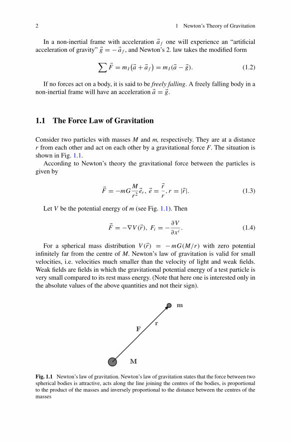
Consider two particles with masses M and m, respectively. They are at a distancer from each other and act on each other by a gravitational force F. The situation isshown in Fig. 1.1.

According to Newton’s theory the gravitational force between the particles isgiven by

�F = −mGM

r2�er , �e = �r

r, r = |�r |. (1.3)

Let V be the potential energy of m (see Fig. 1.1). Then

�F = −∇V (�r), Fi = − ∂V

∂xi. (1.4)

For a spherical mass distribution V (�r) = −mG(M/r) with zero potentialinfinitely far from the centre of M. Newton’s law of gravitation is valid for smallvelocities, i.e. velocities much smaller than the velocity of light and weak fields.Weak fields are fields in which the gravitational potential energy of a test particle isvery small compared to its rest mass energy. (Note that here one is interested only inthe absolute values of the above quantities and not their sign).

Fig. 1.1 Newton’s law of gravitation. Newton’s law of gravitation states that the force between twospherical bodies is attractive, acts along the line joining the centres of the bodies, is proportionalto the product of the masses and inversely proportional to the distance between the centres of themasses

1.1 The Force Law of Gravitation 3

mGM

r� mc2 ⇒ r � GM

c2. (1.5)

The Schwarzschild radius for an object with mass M is RS = 2GM/c2. Hence,far outside the Schwarzschild radius the gravitational field is weak. To get a feelingfor the magnitudes, you may insert the mass of the earth. Then you find that theSchwarzschild mass of the Earth is 9 mm. Comparing with the radius of the Earth,which is RE ≈ 6400 km, we may conclude that the gravitational field is weak on thesurface of the Earth. Similarly the Schwarzschild radius of the Sun is 3 km and theEarth is about 150 million km from the Sun. Hence the gravitational field of the Sunis very weak in most parts of the solar system. This explains, in part, the success ofNewtonian gravity for describing the motion of bodies in the gravitational field ofthe Earth and the Sun.

Example 1.1 (Two particles falling towards each other) Two point particles withmasses m1 and m2 are instantaneously at rest at a distance r0 from each other inempty space, with no other forces present than the gravitational force between them.

How long time will they fall before they collide?Newton’s 2. law is valid with reference to an inertial frame. Hence we start by

introducing a coordinate system fixed with respect to the mass centre of the particles.In this system particles 1 and 2 have coordinates r1 and r2, respectively. The equationsof motion of the two particles are

r1 = Gm2

(r2 − r1)2 , r2 = −G

m1

(r2 − r1)2 . (1.6)

where a dot denotes differentiation with respect to time. Subtracting the equationsand introducing the distance r = r2 − r2 between the particles as a new coordinate,we get the differential equation

r2 r + G(m1 + m2) = 0. (1.7)

Writing this as

r r = −G(m1 + m2)

r2r (1.8)

and integrating with the boundary condition that r = 0 for r = r0, we get the energyconservation equation

r2 = 2G(m1 + m2)

(1

r− 1

r0

). (1.9)

Hence, the falling time is given by the integral

4 1 Newton’s Theory of Gravitation

t =√

r02G(m1 + m2)

r0∫

0

√r

r0 − rdr. (1.10)

Performing the integration gives

t = π

2

r3/20√2G(m1 + m2)

. (1.11)

Assume that the particles have a mass equal to 1 kg and starts 1 m from eachother. Then the falling time is 26.5 h. This illustrates that gravity is indeed a veryweak force.

1.2 Newton’s Law of Gravitation in Local Form

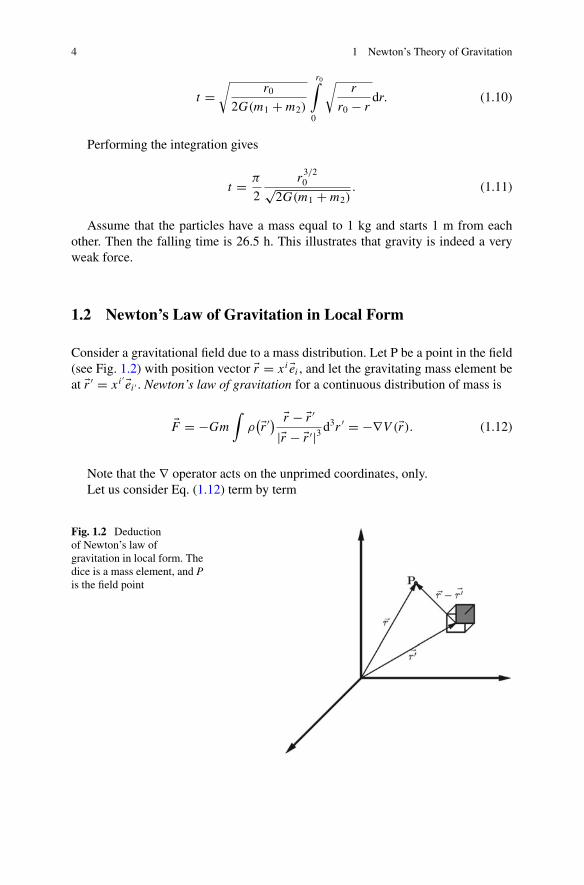
Consider a gravitational field due to a mass distribution. Let P be a point in the field(see Fig. 1.2) with position vector �r = xi �ei , and let the gravitating mass element beat �r ′ = xi

′ �ei ′ . Newton’s law of gravitation for a continuous distribution of mass is

�F = −Gm∫

ρ(�r ′) �r − �r ′

|�r − �r ′|3 d3r ′ = −∇V (�r). (1.12)

Note that the ∇ operator acts on the unprimed coordinates, only.Let us consider Eq. (1.12) term by term

Fig. 1.2 Deductionof Newton’s law ofgravitation in local form. Thedice is a mass element, and Pis the field point

1.2 Newton’s Law of Gravitation in Local Form 5

∇ 1

|�r − �r ′| = �ei ∂

∂xi

1[(x j − x ′ j)

(x j − x ′

j

)]1/2 = �ei ∂

∂xi

[(x j − x ′ j)(x j − x ′

j

)]−1/2

= �ei(

−1

2

)[(x j − x ′ j)(x j − x ′

j

)]−3/22(xk − x ′k)∂xk

∂xi

= −�ei(xk − x ′k)δik[(

x j − x ′ j)(x j − x ′

j

)]3/2 = −(xi − x ′i)�ei

[(x j − x ′ j)

(x j − x ′

j

)]3/2

= − �r − �r ′

|�r − �r ′|3 (1.13)

Equations (1.12) and (1.13) imply

V (�r) = −Gm∫

ρ(�r ′)

|�r − �r ′|d3r ′. (1.14)

Hence, the gravitational potential at the point P is

φ(�r) ≡ V (�r)m

= V (�r) = −G∫

ρ(�r ′)

|�r − �r ′|d3r ′. (1.15)

It follows that

∇φ(�r) = −G∫

ρ(�r ′) �r − �r ′

|�r − �r ′|3 d3r ′, (1.16)

and

∇2φ(�r) = −G∫

ρ(�r ′)∇ · �r − �r ′

|�r − �r ′|3 d3r ′. (1.17)

We now calculate the divergence in the integrand

∇ · �r − �r ′

|�r − �r ′|3 = ∇ · �r|�r − �r ′|3 + (�r − �r ′) · ∇ 1

|�r − �r ′|3 = 3

|�r − �r ′|3 − (�r − �r ′)

· 3(�r − �r ′)

|�r − �r ′|5 = 3

|�r − �r ′|3 − 3

|�r − �r ′|3 = 0, �r �= �r ′. (1.18)

The condition �r �= �r ′ means that the field point is outside the mass distribution.Hence, the Newtonian potential at a point in a gravitational field outside a massdistribution satisfies the Laplace equation

∇2φ = 0. (1.19)

6 1 Newton’s Theory of Gravitation

We shall now generalize this to the case where the field point may be inside amassdistribution. It will then be useful to utilize the Dirac delta function. This functionhas the following properties.

δ(�r − �r ′) = 0, for �r �= �r ′, (1.20)

∫δ(�r − �r ′)d3r ′ =

{1 if �r = �r ′ is contained in the integration region.0 if �r = �r ′ is not contained in the integration region.

(1.21)

∫f(�r ′)δ

(�r − �r ′)d3r ′ = f (�r). (1.22)

A calculation of the integral (1.17) which is valid also in the case where the fieldpoint is inside the mass distribution is obtained by utilizing Gauss integral theorem,

∫

V

∇ · �Ad3r ′ =∮

S

�A · d�S, (1.23)

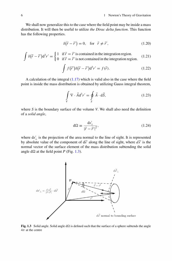
where S is the boundary surface of the volume V. We shall also need the definitionof a solid angle,

d� ≡ ds ′⊥

|�r − �r ′|2 , (1.24)

where ds ′⊥ is the projection of the area normal to the line of sight. It is represented

by absolute value of the component of d�s ′ along the line of sight, where d�s ′ is thenormal vector of the surface element of the mass distribution subtending the solidangle d� at the field point P (Fig. 1.3).

Fig. 1.3 Solid angle. Solid angle d� is defined such that the surface of a sphere subtends the angle4π at the centre

1.2 Newton’s Law of Gravitation in Local Form 7

Applying the Gauss integral theorem we have

∫

V

∇ · �r − �r ′

|�r − �r ′|3 d3r ′ =

∮

S

�r − �r ′

|�r − �r ′|3 · d�s ′ =∮

S

ds ′⊥

|�r − �r ′|2 =∮

S

dΩ (1.25)

Hence

∫

V

∇ · �r − �r ′

|�r − �r ′|3 d3r ′ =

{4π if P is inside themass distribution0 if P is outside themass distribution

. (1.26)

This may be written in terms of the Dirac delta function as

∫

V

∇ · �r − �r ′

|�r − �r ′|3 d3r ′ = 4πδ

(�r − �r ′). (1.27)

We now have

∇2φ(�r) = −G∫

ρ(�r ′)∇ · �r − �r ′

|�r − �r ′|3 d3r ′ = G

∫ρ(�r ′)4πδ

(←r − �r ′

)d3r ′

= 4πGρ(�r), (1.28)

showing that the Newtonian gravitational potential obeys the Poisson equation. Thismeans that Newton’s gravitational theory can be expressed in the following way:

• Mass generates a gravitational potential according to

∇2φ = 4πGρ. (1.29)

• The gravitational potential generates acceleration of gravity �g according to

�g = −∇φ. (1.30)

1.3 Newtonian Incompressible Star

We shall apply Eqs. (1.29) and (1.30) to calculate the gravitational field of a New-tonian incompressible star. Let the gravitational potential be φ(r). In the sphericallysymmetric case Eq. (1.29) then takes the form

8 1 Newton’s Theory of Gravitation

1

r2d

dr

(r2

dφ

dr

)= 4πGρ. (1.31)

Assuming that ρ = constant and integrating gives

r2dφ

dr= 4π

3Gρr3 + K1 = M(r) + K1. (1.32)

whereM(r) is the mass inside a sphere with radius r. According to Eq. (1.30) thegravitational acceleration is

�g = −∇φ = −dφ

dr�er , (1.33)

or

g = M(r)

r2+ K1

r2= 4π

3Gρr + K1

r2. (1.34)

Finite g in r = 0 gives K1 = 0

g = 4π

3Gρr,

dφ

dr= 4π

3Gρr. (1.35)

Assume that the mass distribution has a radius R. A new integration then leads to

φ = 2π

3Gρr2 + K2. (1.56)

Demanding continuous potential at r = R gives.

2π

3GρR2 + K2 = M(R)

R= −4π

3GρR2. (1.37)

Hence

K2 = −2πGρR2. (1.38)

Thus the potential inside the mass distribution is

φ = 2π

3Gρ(r2 − 3R2). (1.39)

The star is in hydrostatic equilibrium that is the pressure forces are in equilibriumwith the gravitational forces.

Consider a mass element dm = ρdV = ρdAdr, in the shell drawn in Fig. 1.4.The pressure force on the mass element is dF = dAdp, and the gravitational

force is