Embed Size (px)
Citation preview
8/21/2019 zhangxc_1
http://slidepdf.com/reader/full/zhangxc1 1/178
MULTISCALE MODELING OF LI-ION CELLS: MECHANICS, HEAT
GENERATION AND ELECTROCHEMICAL KINETICS
by
Xiangchun Zhang
A dissertation submitted in partial fulfillment
of the requirements for the degree ofDoctor of Philosophy
(Mechanical Engineering)
in The University of Michigan2009
Doctoral Committee:
Professor Ann Marie Sastry, Co-Chair
Professor Wei Shyy, Co-Chair
Professor James R. BarberProfessor Levi T. Thompson Jr

8/21/2019 zhangxc_1
http://slidepdf.com/reader/full/zhangxc1 2/178
©Xiangchun Zhang
All Rights Reserved2009

8/21/2019 zhangxc_1
http://slidepdf.com/reader/full/zhangxc1 3/178
ii
To My Parents Xueqin Liu and Lixian Zhang

8/21/2019 zhangxc_1
http://slidepdf.com/reader/full/zhangxc1 4/178
iii
ACKNOWLEDGEMENTS
First of all, I would like to express my grateful thanks to my research advisors
Professor Ann Marie Sastry and Professor Wei Shyy for their guidance and support. I am
very grateful that they led me into this interesting and important topic of Li-ion battery
research that is the key to solving global energy and environmental problems. I appreciate
the opportunity I had to work with these two true scholars and professionals. From the
wonderful experience working with my two advisors, I learned fundamental science and
engineering and also professional skills.
Many thanks go to my committee members, Prof. Levi T. Thompson and Prof.
James R. Barber, for serving on my committee and providing valuable advice on my
thesis.
I would also like to thank the current and former members of both Sastry group
and Shyy group, Dr. Fabio Albano, Dr. Hikaru Aono, Dr. Yen-Hung Chen, Mr. Young-
Chang Cho, Mr. Myoungdo Chung, Mr. Wenbo Du, Mr. Sangwoo Han, Mr. Ez Hassan,
Dr. Munish V. Inamdar, Ms. Qiuye Jin, Mr. Chang-Kwon Kang, Dr. HyonCheol Kim,
Mr. Chih-Kuang Kuan, Dr. Jonghyun Park, Dr. Myounggu Park, Dr. Jeong Hun Seo, Mr.
Jaeheon Sim, Mr. Dong Hoon Song, Mr. Emre Sozer, Dr. Jian Tang, Mr. Patrick Trizila,
Mr. Chien-Chou Tseng, Mr. Peter Verhees, Dr. Chia-Wei Wang, Mr. Seokjun Yun, and
Mr. Min Zhu, for their support and sharing wonderful moments during the past years.
I really appreciate the help from Ms. Lisa Szuma and Ms. Eve Bernos for meeting

8/21/2019 zhangxc_1
http://slidepdf.com/reader/full/zhangxc1 5/178
iv
scheduling and other administrative matters.
I specially thank Dr. Tushar Goel and Mr. Felipe A. C. Viana for the help on
using Surrogate Toolbox.
I gratefully acknowledge the support of my research sponsors, including the U.S.
Department of Energy through the BATT program (Dr. Tien Duong, Program Manager),
Ford Motor Company (Mr. Ted Miller and Mr. Kent Snyder, Program Managers), NASA
under the Constellation University Institute Program (CUIP) (Ms. Claudia Meyer,
program monitor), and General Motors Corporation (Mr. Bob Kruse, GM/UM ABCD
Co-Director).

8/21/2019 zhangxc_1
http://slidepdf.com/reader/full/zhangxc1 6/178
v
TABLE OF CONTENTS
DEDICATION................................................................................................................... ii
ACKNOWLEDGEMENTS ............................................................................................ iii
LIST OF TABLES ......................................................................................................... viii
LIST OF FIGURES ......................................................................................................... ix
LIST OF SYMBOLS ....................................................................................................... xi
LIST OF ABBREVIATIONS ....................................................................................... xiv
ABSTRACT ......................................................................................................................xv
CHAPTER I. INTRODUCTION .....................................................................................1
LI-ION BATTERY TECHNOLOGY: A SOLUTION TO GLOBAL ENERGY AND
ENVIRONMENT PROBLEMS .............................................................................................. 1
LI-ION BATTERY RESEARCH OVERVIEW ...................................................................... 3
Selected Research on Novel Materials ............................................................................ 5
Selected Research on Cell Diagnosis and Testing ........................................................... 8
Selected Research on Cell Modeling, Simulations and Optimization ........................... 10
STRESS AND HEAT GENERATION INSIDE ELECTRODE PARTICLES ..................... 10
MULTISCALE MODELING OF LI-ION BATTERIES ...................................................... 13
Homogenization Approach ............................................................................................ 15
Volume Averaging ........................................................................................................ 16
Scale Bridging ............................................................................................................... 18
SURROGATE-BASED MODELING AND ANALYSIS .................................................... 20
SCOPE AND OUTLINE OF THE DISSERTATION ........................................................... 29
BIBLIOGRAPHY .................................................................................................................. 30
CHAPTER II. NUMERICAL SIMULATION OF INTERCALATION-INDUCED
STRESS IN LI-ION BATTERY ELECTRODE PARTICLES ...................................36

8/21/2019 zhangxc_1
http://slidepdf.com/reader/full/zhangxc1 7/178
vi
INTRODUCTION ................................................................................................................. 36
METHODS ............................................................................................................................ 39
Stress-Strain Relations ................................................................................................... 39
Diffusion Equation ........................................................................................................ 41
Numerical Methods ....................................................................................................... 43
Material Properties ........................................................................................................ 47
RESULTS AND DISCUSSION ............................................................................................ 49
1D Finite Difference Simulations .................................................................................. 49
3D Finite Elements Simulation Results ......................................................................... 54
CONCLUSION...................................................................................................................... 63
BIBLIOGRAPHY .................................................................................................................. 64
CHAPTER III. SURROGATE-BASED ANALYSIS OF STRESS AND HEAT
GENERATION WITHIN SINGLE CATHODE PARTICLES UNDERPOTENTIODYNAMIC CONTROL .............................................................................66
INTRODUCTION ................................................................................................................. 66
ELECTROCHEMICAL, MECHANICAL AND THERMAL MODELING ........................ 69
Model of Intercalation ................................................................................................... 71
Intercalation-Induced Stress Model ............................................................................... 75
Heat Generation Model ................................................................................................. 77
Spherical Particle Simulation Results ............................................................................ 80
SURROGATE-BASED ANALYSIS OF ELLIPSOIDAL PARTICLES UNDER
DIFFERENT CYCLING RATES ......................................................................................... 88
Selection of Variables And Design of Experiments ...................................................... 91
Model Construction and Validation............................................................................... 94
Analysis Based on Obtained Surrogate Models ............................................................ 97
ASSUMPTION OF A UNIFORM ELECTRIC POTENTIAL ........................................... 100
CONCLUSIONS ................................................................................................................. 104
BIBLIOGRAPHY ................................................................................................................ 106
CHAPTER IV. SURROGATE-BASED SCALE BRIDGING AND MICROSCOPIC
SCALE MODELING OF CATHODE ELECTRODE MATERIALS .....................110
INTRODUCTION ............................................................................................................... 110
Challenges for Li-Ion Battery Modeling ..................................................................... 110
Review of the Existing Li-Ion Battery Modeling Work in the Literature ................... 112
The Objectives of This Study ...................................................................................... 115

8/21/2019 zhangxc_1
http://slidepdf.com/reader/full/zhangxc1 8/178
vii
METHODS .......................................................................................................................... 116
Li-Ion Cell Cycling Mechanisms and Governing Equations on Microscopic Scale ... 116
Multiscale Modeling Framework ................................................................................ 121
3D Microscopic Modeling of Electrode Particle Clusters ........................................... 129
Surrogate-Based Scale Bridging .................................................................................. 133
Summary of the Multiscale Modeling Framework ...................................................... 136
RESULTS AND DISCUSSION .......................................................................................... 138
Analysis of 3D Microscopic Simulation Results ......................................................... 138
Effective Material Property Calculations .................................................................... 146
Surrogate Model Construction for Reaction Current Density ..................................... 148
CONCLUSIONS ................................................................................................................. 152
BIBLIOGRAPHY ................................................................................................................ 155
CHAPTER V. CONCLUSIONS AND FUTURE WORK..........................................158
8/21/2019 zhangxc_1
http://slidepdf.com/reader/full/zhangxc1 9/178
viii
LIST OF TABLES
Table 1.1: Comparison of key battery technologies.. ...................................................................... 2
Table 2.1: Stress and strain in cathode materials in the intercalation process.. ............................. 37
Table 2.2: Material properties of Mn2O4.. ...................................................................................... 48
Table 3.1: Representative cathode compositions and particle sizes.. ............................................ 70
Table 3.2: Parameters and material properties for the intercalation model (where r 0 is the radius of
a spherical particle).. ...................................................................................................................... 76
Table 3.3: Averaged heat generation rates during charge process.. ............................................... 90
Table 3.4: Design variables and design space.. .............................................................................. 93
Table 3.5: Evaluation of the response surface approximations...................................................... 96
Table 3.6: Global sensitivity indices (total effect) for stress and resistive heat.. ........................ 101
Table 4.1: Characteristic time scales for physicochemical processes inside a Li-ion battery...... 113
Table 4.2: Material properties for 3D microscopic scale simulations.......................................... 132
Table 4.3: Input variables and their range for 3D microscopic scale simulations.. ..................... 135
Table 4.4: Comparison of simulation results from pseudo 2D and 3D microscopic models.. ..... 142
Table 4.5: Ratio between effective and bulk (intrinsic) transport properties.. ............................. 147
Table 4.6: Evaluation of the constructed surrogate models.. ....................................................... 149
Table 4.7: Global sensitivity indices calculated from kriging model. ......................................... 153

8/21/2019 zhangxc_1
http://slidepdf.com/reader/full/zhangxc1 10/178
ix
LIST OF FIGURES
Figure 1.1: Schematic diagram of a Li-ion cell ............................................................................... 4
Figure 1.2: EV commercialization Li-ion battery technology spider chart...................................... 6
Figure 1.3: Experimental observation of fracture in cathode particles: (a) LiFePO4 particle after
60 cycles [24]; (b) gold-codeposited LiMn2O4 electrode particles after cyclic voltammetric tests at
a scan rate of 4mV/s [25]; (c)LiCoO2 particles after 50 cycles [26]. ............................................. 12
Figure 1.4: Summary of scale bridging approaches. ...................................................................... 19
Figure 1.5: Surrogate modeling: (a) key steps of surrogate modeling; (b) design of experiments by
FCCD; (c) design of experiments by LHS. .................................................................................... 22
Figure 1.6: An example of various surrogate models constructed based on training data obtained
from the analytical function y=exp( x4). .......................................................................................... 25
Figure 2.1: Comparison of simulation results of two models. ....................................................... 50
Figure 2.2: Maximum dimensionless radial stress versus dimensionless current density. ............ 51Figure 2.3: Numerical results for the effects of stress. .................................................................. 53
Figure 2.4: Convergence plot of finite element solutions for: (a) hydrostatic stress and (b)
concentration. ................................................................................................................................. 55
Figure 2.5: Schematic of an ellipsoidal particle, with coordinate system. ..................................... 57
Figure 2.6: Solutions at the end of discharge for an ellipsoid of aspect ratio 1.953, (a)
concentration, (b) von Mises stress, and (c) shear stress .............................................................. 58
Figure 2.7: Maximum von Mises stress during discharge, for various ellipsoids .......................... 59
Figure 2.8: The effect of aspect ratio, for fixed particle volume ................................................... 60
Figure 2.9: The effect of aspect ratio, for fixed shorter semi axes. ................................................ 62
Figure 3.1: Potentials: (a) OCP of LiMn2O4 and (b) applied potential sweeping profile during one
cycle.. ............................................................................................................................................. 74
Figure 3.2: Material properties: (a) the derivative of OCP over temperature: curve fitting of the
measured data from Ref. 20, and (b) the derivative of partial molar enthalpy over concentration
obtained by ( )d / d H c F U T u T c∂ ∂ ∂ ∂ = − − based on the curve fit in (a).................................. 79
Figure 3.3: Simulation results of a spherical particle with 0.4mV/sv = , 0 5r mμ = : (a) diffusion
flux on the particle surface, (b) radial stress at the center of the particle, and (c) von Mises stress
on the particle surface.. .................................................................................................................. 81Figure 3.4: Simulation results of a spherical particle in the charge half cycle ( 0.4mV/sv = ,
0 5r mμ = ): (a) reaction flux on the particle surface, (b) von Mises stress on the particle surface,
(c) surface overpotential, and (d) exchange current density (divided by Faraday’s constant). ...... 83
Figure 3.5: Distribution of lithium-ion concentration inside a spherical particle at different time
instants during the charge half cycle.. ............................................................................................ 85
8/21/2019 zhangxc_1
http://slidepdf.com/reader/full/zhangxc1 11/178
x
Figure 3.6: Simulation results of a spherical particle under 20C charge: (a) reaction flux on the
particle surface, and (b) von Mises stress on the particle surface.. ................................................ 87
Figure 3.7: Simulation results of various heat generation sources during the charge half cycle: (a)
resistive heating, (b) entropic heating, and (c) heat of mixing.. ..................................................... 89
Figure 3.8: Geometric illustration of an ellipsoidal particle.. ........................................................ 92
Figure 3.9: The dependency between objective functions and design variables (a) maximum von
Mises stress (in megapascal), (b) time-averaged resistive heat rate (in picowatts).. ..................... 98
Figure 3.10: Simulation with a predescribed potential variation: (a) potential variation on particle
surface at t=1534s, (b) time history of von Mises stress on particle surface, (c) concentration
distribution inside the particle at t=1534s, and (d) von Mises stress distribution inside the particle
at t=1534s.. ................................................................................................................................... 103
Figure 4.1: Scales in Li-ion batteries: (a) dimension for a single cell, (b) components and their
dimensions inside a single cell along the thickness direction, and (c) a SEM image for LiMn2O4
positive electrode.. ....................................................................................................................... 111
Figure 4.2: Surrogate-based scale bridging for multiscale modeling framework.. ...................... 130
Figure 4.3: Summary of the multiscale framework. .. ................................................................. 137
Figure 4.4: Generated microstructure: (a) liquid phase of electrolyte, (b) solid phase of active
material, and (c) the whole simulation domain containing both phases.. .................................... 139
Figure 4.5: Results of a 3D microscopic scale simulation: (a) Li-ion concentration in the solid
phase (mol/m3), (b) Li-ion concentration in the liquid phase (mol/m3), and (c) reaction current
density at the phase interface (A/m2).. ......................................................................................... 140
Figure 4.6: Comparison of (normalized) reaction current density: (a) the temporal variation for
pseudo 2D and 3D microscopic models, (b) distribution of reaction current density (A/m2) at
t=10.77min by 3D microscopic model, and (c) distribution of reaction current density (A/m2) at
t=26.16min by 3D microscopic model.. ....................................................................................... 145
Figure 4.7: Histogram of surrogate model prediction errors on 21 testing points.. ..................... 151

8/21/2019 zhangxc_1
http://slidepdf.com/reader/full/zhangxc1 12/178
xi
LIST OF SYMBOLS
a , b , c lengths of the three semi-axes of ellipsoid μ m
a specific interfacial area m2/m
3 (or m
-1)
c concentration of lithium ions -3mmol
c~ concentration change from initial value -3mmol
C p
heat capacity J/(mol-kg)
D lithium diffusion coefficient 12 sm −
E Young’s modulus GPa
F Faraday’s constant -1molC96487
f molar activity coefficient of the electrolyte
g s volume fraction of phase s
H Δ enthalpy of reaction -1molJ
H partial molar enthalpy -1molJ
I dimensionless current density
I current of cell A
ni ( ni ) current density vector (scalar) -2mA
0i exchange current density -2mA
J ( J ) species flux vector (scalar) -1-2 smmol
k reaction constant 1/215/2 molsm −−
xk , yk , z k thermal conductivity W/(K-m)
M mobility ( )2m mol J s A⋅ ⋅
N s number of sampling points
N v dimension of the design space
Q heat transfer/generation rate W

8/21/2019 zhangxc_1
http://slidepdf.com/reader/full/zhangxc1 13/178
xii
R gas constant -1-1 K molJ314.8
R equivalent radius of ellipsoidal particles μ m
adj R 2 adjusted coefficient of multiple determination
0r particle radius μ m
k r rate of reaction k -1smol
T temperature K
t time s
0
+t transference number
U open circuit potential V
HU enthalpy potential V
u displacement m v ion movement velocity inside solid particles sm
V 1(V 2) electric potential in solid (liquid) phase V
V variance of objective functions in surrogate modeling
v potential sweep rate -1smV
X molar fraction of lithium in the electrode
z y x ,, spatial coordinate μ m
y state of charge
Z systematical departure in the kriging model
Greek symbols
α aspect ratio
β symmetry factor
β coefficients in polynomial response surface
ε a scale parameter ( 1<<ε )
ijε strain
η surface overpotential V
σ 1 conductivity of solid phase s/m
κ conductivity of liquid phase s/m
ν Poisson’s ration

8/21/2019 zhangxc_1
http://slidepdf.com/reader/full/zhangxc1 14/178
xiii
μ chemical potential J/mol
ijσ stress Pa
Ω partial molar volume -13molm
ρ density kg/m
3
Subscripts:
0 exchange current density 0i ; particle radius 0r ; initial concentration 0c
1 solid phase
2 liquid phase
adj adjusted (coefficient of multiple determination)
avg time averaged (heat generation rate)
e entropic heat
g heat generation
h hydrostatic (stress)
i, j index for tensor elements, or index of species
k index for a chemical reaction
l concentration of Li-ion in the electrolyte
max maximum
mixing heat of mixing
r resistive heating
rad radial direction
s concentration of Li-ion in the solid phase
tang tangential direction
v von Mises stress
θ concentration of available vacant sites
Superscripts:
avg average over volume bulk bulk (intrinsic) material properties
eff effective material properties
Others:
^ dimensionless variables

8/21/2019 zhangxc_1
http://slidepdf.com/reader/full/zhangxc1 15/178
xiv
LIST OF ABBREVIATIONS
AFM Atomic Force Microscopy
EC Ethylene Carbonate
EIS Electrochemical Impedance Spectroscopy
EMC Ethyl Methyl Carbonate
EV Electric Vehicle
FCCD Face Centered Central-Composite Design
LHS Latin Hypercube Sampling
OCP Open Circuit Potential
PDE Partial Differential Equation
PRESS Prediction Error Sum of Squares
PRS Polynomial Response Surface
PVdF Poly Vinylidene Fluoride
RBNN Radial Basis Neural Network
REV Representative Elementary Volume
RMS Root Mean SquareRMSE Root Mean Square Error
SEI Solid Electrolyte Interface
SEM Scanning Electron Microscope
USABC United States Advanced Battery Consortium
XPS X-Ray Photoelectron Spectroscopy

8/21/2019 zhangxc_1
http://slidepdf.com/reader/full/zhangxc1 16/178
xv
ABSTRACT
MULTISCALE MODELING OF LI-ION CELLS: MECHANICS, HEAT
GENERATION, AND ELECTROCHEMICAL KINETICS
by
Xiangchun Zhang
Co-Chairs: Ann Marie Sastry and Wei Shyy
To assists implementing Li-ion battery technology in automotive drivetrain
electrification, this study focuses on improving calendar life by reducing degradation due
to stress-induced electrode particle fracture and heat generation, and creating models for
computer simulations that can lead to optimizing battery design.
To improve the calendar life of Li-ion batteries, capacity degradation during
battery cycling has to be understood and minimized. One of the degradation mechanisms
is fracture of electrode particles due to intercalation-induced stress. A model with the
analogy to thermal stress modeling is proposed to determine localized intercalation-
induced stress in electrode particles. Intercalation-induced stress is calculated within
ellipsoidal electrode particles with a constant diffusion flux assumed at the particle
surface. It is found that internal stress gradients significantly enhance diffusion.
Simulation results suggest that it is desirable to synthesize electrode particles with
smaller sizes and larger aspect ratios, to reduce intercalation-induced stress during
cycling of lithium-ion batteries.
8/21/2019 zhangxc_1
http://slidepdf.com/reader/full/zhangxc1 17/178
xvi
Thermal runaway caused by excessive heat generation can lead to catastrophic
failure of Li-ion batteries. Stress and heat generation are calculated for single ellipsoidal
particles under potentiodynamic control. To systematically investigate how stress and
heat generation are affected by electrode particle shape and cycling rate, a surrogate-
based analysis is conducted. It is shown that smaller sizes and larger aspect ratios of
(prolate) particles reduce the heat and stress generation inside electrode particles.
Battery scale modeling is required for optimizing battery design through computer
simulations. To include the electrode microstructure information in battery scale
modeling, a multiscale framework is proposed. The resulting closure terms for
macroscopic scale governing equations derived from the volume averaging technique are
calculated directly from 3D microscopic scale simulations of microstructure consisting of
multiple solid electrode particles and liquid electrolyte. It is shown that 3D microscopic
simulations give different values for closure terms from the traditional pseudo 2D
treatment. To efficiently exchange the information between microscopic and macroscopic
scales, a surrogate-based approach is proposed for scale bridging. The surrogate model
characterizes the interplay between geometric and physical parameters, and is shown to
be able to significantly enhance the macroscopic model.
8/21/2019 zhangxc_1
http://slidepdf.com/reader/full/zhangxc1 18/178
1
CHAPTER I
INTRODUCTION
1. LI-ION BATTERY TECHNOLOGY: A SOLUTION TO GLOBAL ENERGY
AND ENVIRONMENT PROBLEMS
Ground transportation using gasoline engines is a major factor in global energy
and environmental problems. Automotive vehicles contribute a significant portion of the
total carbon emissions around the world. In 2003, an estimated 21 percent of world’s
carbon emissions were generated by the United States. For these 6900 Tg (6.9 billion
tons) CO2 equivalent emissions by the U.S. in 2003, the transportation sector accounted
for approximately 27 percent of the total. 62 percent of the transportation emissions came
from passenger vehicles or light trucks [1]. One solution to energy and environment
problems caused by ground transportation is to electrify automotive drivetrains by
developing hybrid electric, plug-in hybrid, or pure electric vehicles. Analysis shows that
hybrid electric vehicles reduce use phase greenhouse emissions by 30-37% compared to
conventional gasoline vehicles, and plug-in hybrid electric vehicles reduce emissions by
38-41% compared to conventional gasoline vehicles [2 ]. Pure electric vehicles are
considered to produce zero carbon emissions during the use phase.
The major candidates for electric vehicle power sources are fuel cells and
batteries. Fuel cells are less attractive than batteries due to current issues with hydrogen
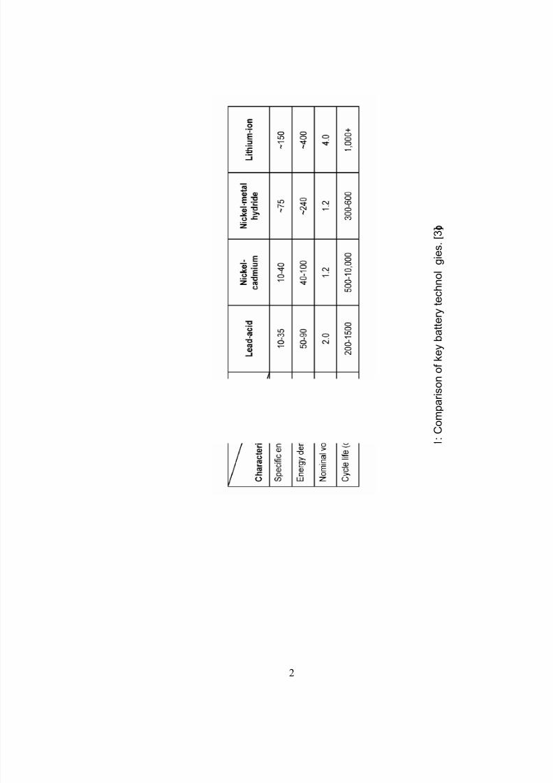
storage and transportation. Table 1.1 shows a comparison of several key battery
8/21/2019 zhangxc_1
http://slidepdf.com/reader/full/zhangxc1 19/178
g i e s .
[ 3 ]
e y b a t t e r y t e c h n o l
1 : C o m p a r i s o n o f k
T a b l e 1 .
2

8/21/2019 zhangxc_1
http://slidepdf.com/reader/full/zhangxc1 20/178
3
technologies [3]. It is shown that Li-ion batteries have superior voltage, energy per unit
mass and per unit volume. For all commercial hybrid vehicles available in the market,
nickel metal hydride batteries are used. As shown in Table 1.1, Li-ion batteries have
twice the specific energy of nickel metal hydride batteries. Other advantages of Li-ion
batteries include no memory effect, broad temperature range of operation, and high rate
and high power discharge capability.
2. LI-ION BATTERY RESEARCH OVERVIEW
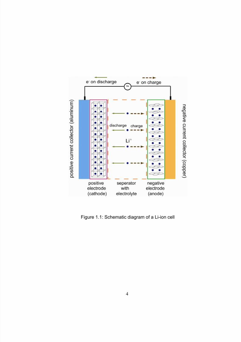
Figure 1.1 illustrates the electrochemical process within a lithium-ion cell. A cell
has one negative and one positive electrode. A separator is used between the two
electrodes to prevent short-circuiting. A current collector is attached to each electrode,
aluminum for positive and copper for negative electrodes respectively. During the
discharge process, lithium ions are extracted from the negative electrode (deintercalation)
and inserted into the positive electrode (intercalation). In the recharge process, lithium
ions move in the opposite direction. Electrons are conducted through the external circuit
corresponding to the movement of lithium ions. The negative electrode of Li-ion batteries
commonly uses carbonaceous materials; recently silicon and Li4Ti5O12 have been
proposed for this use. Common positive electrode materials include LiCoO2, LiNiO2,
LiMn2O4, LiFePO4 and Li(Ni1/3Co1/3Mn1/3)O2. The porous electrodes consist of active
material particles, binders and other additives. The porous configuration of electrodes
provides a high surface area for reactions and reduces the distance between reactants and
the surface where reactions occur. In the intercalation and deintercalation process, the
lattice structure of intercalation hosts changes, causing volume change and strain inside
the electrode. The corresponding stress is called intercalation-induced stress. The porous
8/21/2019 zhangxc_1
http://slidepdf.com/reader/full/zhangxc1 21/178
Figure 1.1: Schematic diagram of a Li-ion cell
4

8/21/2019 zhangxc_1
http://slidepdf.com/reader/full/zhangxc1 22/178
5
electrode and separator is filled with electrolyte for transport of Li ions. An example for
the most commonly used electrolyte is LiPF6 dissolved in carbonate solvents.
Li-ion batteries are widely used in consumer electronics, such as cell phones and
laptop computers, and in military electronics. To successfully implement Li-ion
technology in pure electric vehicles, further improvements for Li-ion technology are
required. The United States Advanced Battery Consortium (USABC) set goals [4] for
advanced batteries for electric vehicles as shown in Figure 1.2. It could be seen that the
current Li-ion battery technology fulfills the requirements of cycle life, power density
and specific power. However, further improvements in energy density, specific energy,
calendar life, operating temperature range and further reduction of cost are required.
Moreover, even though the abuse tolerance goal that could not be quantified is not shown
in Figure 1.2, improvements are necessary for Li-ion batteries’ response to abuse
conditions such as crush, overcharge and overheating. Therefore, to successfully
implement Li-ion technology in electric vehicles, the following issues have to be
addressed: (1) reducing cost, (2) improving calendar life, (3) increasing tolerance to
abusive conditions, and (4) further improving energy per unit volume and mass. To
address these issues, Li-ion battery related research has concentrated on: (1) novel
material synthesis and evaluation, (2) Li-ion cell diagnosis and testing, and (3) cell design
optimization through modeling and simulations. Li-ion battery related research is briefly
reviewed in the following sections.
2.1. Selected Research on Novel Materials
Novel materials for anode, cathode and electrolyte have been synthesized and
evaluated to improve cell performance, life and cost. Carbon materials traditionally used

8/21/2019 zhangxc_1
http://slidepdf.com/reader/full/zhangxc1 23/178
Figure 1.2: EV commercialization Li-ion battery technology spider
“.
Technical Team Technology Development Roadmap” by USABC [4].)
6

8/21/2019 zhangxc_1
http://slidepdf.com/reader/full/zhangxc1 24/178
7
as Li-ion cell anodes give a theoretical capacity 372 mAh/g. To increase this theoretical
capacity, silicon was used as anode material because lithium can alloy with Si up to 4.4
per Si that gives a theoretical capacity of 4200mAh/g. However, the excessive expansion
and contraction of the alloy lattice structure causes material pulverization that leads to
capacity degradation due to loss of electric contact. Nano particles [5] and nanowires [6]
have been proposed to solve the excessive volume expansion problem of silicon as an
intercalation compound. To completely avoid the volume expansion that might lead to
capacity degradation, Li4Ti5O12 was proposed for anodes as a zero-strain insertion
material [7] to improve battery cycle life. Due to the high open circuit potential of
Li4Ti5O12 versus Li, no passivation film is formed during cycling. Therefore, lithium can
be inserted and extracted from the compound at a high rate. However, cells using this
material as anode have lower voltage output.
For cathode materials, layered structure material LiCoO2 was first used for the
first commercial Li-ion cells by Sony Corporation. However, LiCoO2 is expensive and
toxic because of the element cobalt. Other cathode candidate materials have been
proposed and studied, such as LiNiO2, LiMn2O4 [ 8 ], LiFePO4 [ 9 ] and
Li(Ni1/3Co1/3Mn1/3)O2 [ 10 ]. Layer structure material LiNiO2 is thermally instable.
Another layer structure Li(Ni1/3Co1/3Mn1/3)O2 has the combination of nickel, manganese
and cobalt that can provide advantages including higher reversible capacity with milder
thermal stability at charged state and lower cost and less toxicity than LiCoO2. However,
it is difficult to prepare and synthesize this complicated material. Spinel structure
material LiMn2O4 is inexpensive and environmentally benign, but it has the disadvantage
of lower capacity and higher rate of capacity degradation when cycled or stored. Olivine

8/21/2019 zhangxc_1
http://slidepdf.com/reader/full/zhangxc1 25/178
8
structure material LiFePO4 has the advantage of low cost, environmentally benignness,
and relatively high capacity, but has the disadvantage of low electronic conductivity that
results in lower power output. Several approaches were proposed to improve the
electronic conductivity of LiFePO4, such as coating the active material with a thin layer
of carbon [11, 12], and selective doping with supervalent cations [13].
2.2. Selected Research on Cell Diagnosis and Testing
Li-ion cells and battery have been diagnosed and tested to understand (1) the
capacity degradation mechanisms, especially from the aspects of solid-electrolyte
interphase (SEI) [14] and material structural change, and (2) the abuse tolerance of cells
[15].
Solid electrolyte interphase (SEI), a protective passivation film formed on anode
material surfaces during the first charge cycle, decides the retention capacity and storage
life of Li-ion batteries because it creates a barrier between the negative electrode and the
electrolyte that reduces transfer of electrons from the electrodes to the electrolyte and
transfer of solvent molecules and salt anions from the electrolyte to the electrodes. Both
in-situ and ex-situ characterization of SEI layers have been carried out to understand the
formation and composition SEI layers. For example, an ex-situ study by atomic force
microscopy (AFM) and x-ray photoelectron spectroscopy (XPS) revealed the electric
potential-dependent character of the surface-film species formation and evidenced a
process of dissolution/redeposition of SEI layer in the first five cycles [16]. An in-situ
electrochemical impedance spectroscopy approach was used to measure the resistance of
the SEI layer during cell cycling and it was found that addition of vinylene carbonate
(VC) as an additive to LiPF6 –ethylene carbonate/ethyl methyl carbonate (EC/EMC)

8/21/2019 zhangxc_1
http://slidepdf.com/reader/full/zhangxc1 26/178
9
electrolyte solution helps to reduce SEI layer resistance by forming a high quality SEI
film [17].
When active materials of battery electrode undergo electrochemical cycling, they
experience phase change and volume expansion/contraction that affects the battery
performance. Material structural change during battery cycling has been studied
experimentally. For example, an in-situ X-Ray diffraction technique was used to study
the phase changes and regions of phase stability during the lithiation and delithiation of
Si electrodes, and it was found that improved battery cycle life can be obtained if the Si
electrodes are cycled above 70mV [ 18 ]. An in-situ synchrotron X-Ray diffraction
technique was used to study the phase changes of LiMn2O4 cathode materials during cell
cycling to understand the capacity fade caused by inhomogenetity of the spinel local
structure [19]. The study proposed a phase transition model from a lithium-rich phase to a
lithium-deficient phase and finally to a λ-MnO2-like cubic phase, instead of a continuous
lattice constant contraction in a single phase.
To improve the calendar life of Li-ion cells, cell testing has been conducted to
understand aging phenomena and mechanisms. For example, electrochemical testing of
different cell designs with different shapes and cathode materials showed that extra
lithium (or lithium reserve) for nickel-based oxides as cathode materials enhances the
calendar life of batteries [20].
Abuse tolerance of Li-ion batteries is a major concern limiting their applications.
Abuse can be categorized as physical abuse (crush and nail penetration), electrical abuse
(short circuit and overcharge), and thermal abuse (overheating). Thermal abuse can occur
during relatively normal operating conditions when excessive heat generated is not

8/21/2019 zhangxc_1
http://slidepdf.com/reader/full/zhangxc1 27/178
10
efficiently dissipated. This condition can eventually cause catastrophic failure of batteries
along with ignition of battery active materials, so called thermal runaway. Many cell
testing studies have been conducted to understand battery abuse tolerance. For example,
an experimental study with cycling of high power 18650 cells was carried out to study
the contribution of individual cell components to overall cell thermal abuse tolerance
[21]. It was found that microcarbon mesobeads increase thermal stability of cells due to
more effective solid electrolyte interface formation.
2.3. Selected Research on Cell Modeling, Simulations and Optimization
Li-ion cell models have been developed for computer simulations and battery
design optimization. For example, a pseudo 2D model was used to numerically study the
effect of cathode thickness and electrode porosity on energy and power output of Li-ion
cells [22]. A coupled electrochemical and thermal model was developed to study heat
transfer and thermal management of lithium polymer batteries [23 ]. In this study,
electrochemical and thermal behavior of batteries was studied under different discharge
temperatures. Current and active material particle size and several thermal management
systems approaches were discussed to prevent overheating of batteries.
This study will focus on (1) improving calendar life by reducing performance
degradation due to stress induced electrode particle fracture and heat generation through
modeling and numerical simulations, and (2) creating models including electrode
materials microstructural information for computer simulations that can lead to
optimizing battery design for improved energy output per unit volume and mass.
3. STRESS AND HEAT GENERATION INSIDE ELECTRODE PARTICLES

8/21/2019 zhangxc_1
http://slidepdf.com/reader/full/zhangxc1 28/178
11
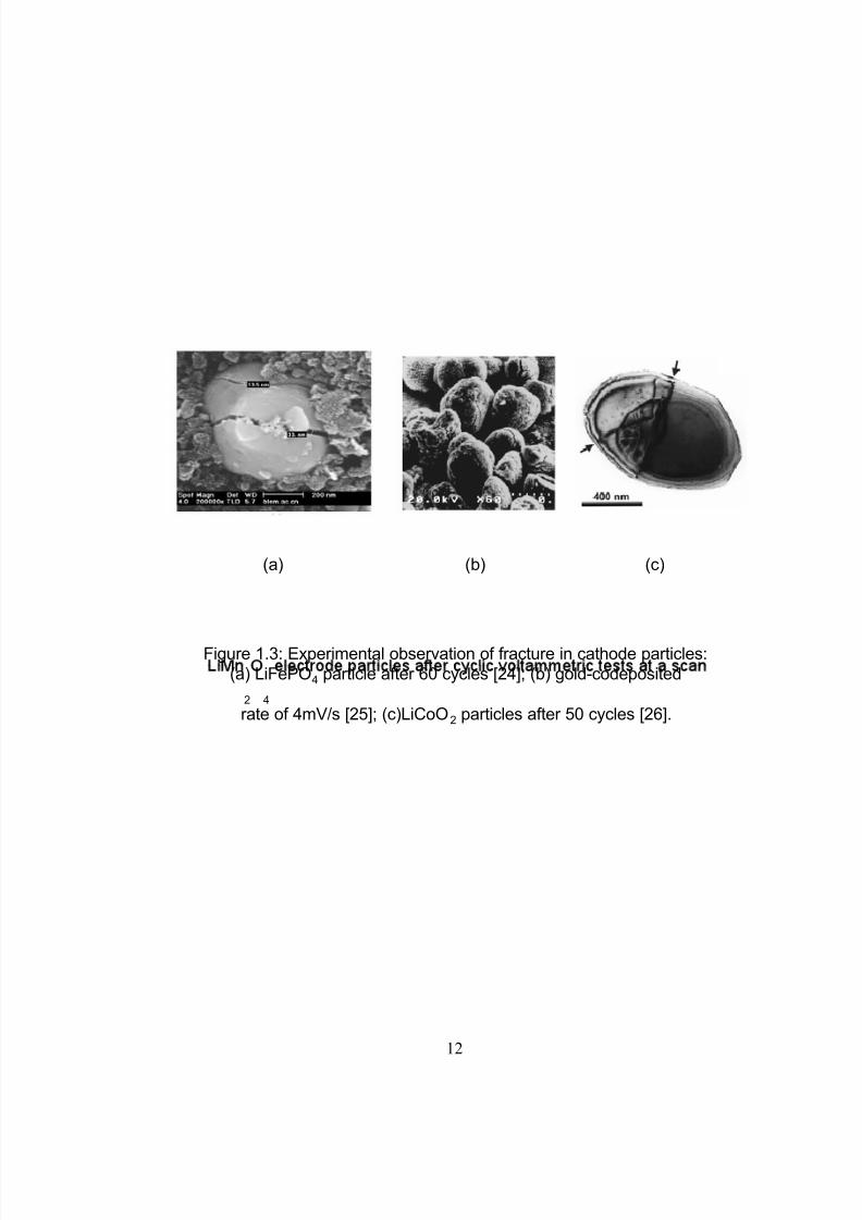
To improve the calendar life of Li-ion batteries, capacity degradation during
battery cycling has to be understood and minimized. One of the capacity degradation
mechanisms is fracture of electrode particles due to intercalation-induced stress. Fracture
has been experimentally [24 ][25][26] observed in cathode particles of lithium-ion
batteries after a relatively small number of cycles as shown in Figure 1.3. When Li ions
are intercalated into the lattice of active material in electrodes, the lattice is expanded
accordingly. This lattice expansion causes strain inside the material. Non-uniform strain
results in stress, the so-called intercalation-induced stress. As Li ions are inserted and
extracted during cycling of batteries, the intercalation compound undergoes cyclic load of
intercalation-induced stress. This eventually causes electrode particle fracture after a
certain number of discharge/charge cycles. Particle-scale fracture of active materials
results in battery performance degradation due to the loss of electrical contact and
subsequent increase in the surface area subjected to side reactions [27].
To predict the intercalation-induced stress in electrode materials, a model is
needed. A one-dimensional model was developed to estimate stress generation within
spherical electrode particles [28]. However, this model does not predict three dimensional
stresses inside three dimensional electrode particles. Therefore, a three dimensional
model based on the thermal stress analogy, following the treatment of diffusion-induced
stress by analogy to thermal stresses first proposed by Prussin [29], will be proposed in
this study to simulate the intercalation-induced stresses inside ellipsoidal particles.
Heat generation inside batteries is a major safety concern because excessive heat
generation in Li batteries, resulting in thermal runaway, results in complete cell failure
8/21/2019 zhangxc_1
http://slidepdf.com/reader/full/zhangxc1 29/178
Figure 1.3: Experimental observation of fracture in cathode particles:
(a) LiFePO4 particle after 60 cycles [24]; (b) gold-codeposited
(a) (b) (c)
2 4
rate of 4mV/s [25]; (c)LiCoO2 particles after 50 cycles [26].
12
8/21/2019 zhangxc_1
http://slidepdf.com/reader/full/zhangxc1 30/178
13
accompanied by violent venting and rupture, along with ignition of battery active
materials. Heat generation inside batteries comes from irreversible resistive heating,
reversible entropic heat, heat change of chemical side reactions, and heat of mixing due
to the generation and relaxation of concentration gradients [30].
To date, there has been no study in the literature on how to design electrode
particles to reduce both stress and heat generation. In this study, a surrogate-based
approach is used to systematically study the effect of both particle shape and cycling
parameter on stress and heat generation inside single ellipsoidal cathode particles under
potentiodynamic control and to provide design guidelines for reducing stress and heat
generation. Experiments [31] and simulations [32] have been conducted using a single
particle electrode to study the kinetic and transport properties of Li ion intercalation and
deintercalation. The single particle electrode model is extended in this study to include
stress and heat generation analysis.
4. MULTISCALE MODELING OF LI-ION BATTERIES
Li-ion battery models in the existing literature with different fidelity include
equivalent-circuit-based models, physics-based pseudo 2D models, and a mesoscale 3D
model. Equivalent-circuit-based models, which originated from conventional
electrochemical impedance spectroscopy (EIS) battery characterization techniques, use
an equivalent electric circuit composed of resistors and capacitors to simulate cell
performance and behavior [33, 34, 35]. Pseudo 2D models were first developed from
porous electrode theory [36] by solving continuum scale governing equations for all the
physicochemical processes over homogeneous media along the thickness direction of a
cell [37]. The required effective material properties are commonly modeled by the

8/21/2019 zhangxc_1
http://slidepdf.com/reader/full/zhangxc1 31/178
14
classical Bruggeman’s equation. The volumetric reaction rate is calculated using a
simplified separated spherical electrode particle by introducing a pseudo dimension. A
mesoscale modeling approach was proposed to implement the 3D detailed modeling of
electrode materials consisting of regularly and randomly arranged cathode particles [38].
However, the number of electrode particles included in the model was limited due to the
excessive computation power requirement.
Scales inside a Li-ion cell span from microns for electrode particles to millimeters
for cell thickness. To successfully include electrode microstructure information in a
battery scale model, a multiscale framework is needed. The main objective of multiscale
modeling is to capture the physics to a certain desired accuracy in an efficient way.
Microscopic models (for electrode microstructure) are accurate but computationally
expensive, while macroscopic models (for a Li-ion cell) are simplified and efficient. The
combinational use of models on these two scales will help to achieve accuracy and
efficiency at the same time.
Microscopic and macroscopic models could be fundamentally different in terms
of the physics principles applied. For example, one could apply molecular dynamics to
the microscopic scale and continuum fluid dynamics to the macroscopic scale.
Sometimes, one basic physics principle is applicable for all scales and the scale disparity
is caused by geometric complexity, which is the case for the processes in porous battery
electrode materials. For multiscale modeling of the processes in porous media, there are
two approaches to derive the macroscopic governing equations from their counterparts on
the microscopic scale, volume averaging [39] and homogenization [40][41].

8/21/2019 zhangxc_1
http://slidepdf.com/reader/full/zhangxc1 32/178
15
4.1. Homogenization Approach
The homogenization approach is an upscaling procedure that lets the microscopic
scale approach zero asymptotically. A systematic way of performing this approach is to
do asymptotic expansion of variables.
To illustrate the basic idea of homogenization, the following diffusion equation is
used.
( ) ( ) ( )
( ) ( )
30,
, D
D c f
c c
ε ε ⎧ ⎡ ⎤∇ ⋅ ∇ + = ∈ Ω ⊂⎪ ⎣ ⎦⎨
= ∈ ∂Ω⎪⎩
x x x x R
x x x. (1)
It is assumed that the diffusion coefficient Dε
is rapidly oscillating, and it is of the
form ( ) D D xε
ε = , where function D is periodic (with periodicity smaller than unity)
and ε a scale parameter ( 1<<ε ). With this assumption, the diffusion coefficient of
porous media changes periodically from pores and solid matrix. Define a new variable
ε /xy = . y is the coordinate for the microscale, and it is commonly called fast variable
( x is often referred as slow variable). All variables should depends on the coordinates
( x and y ) for both scales. Therefore, we can do the asymptotic expansion with respect to
ε
( ) ( ) ( ) ( )2
0 1 2, , ,c c c cε ε ε = + + +x x y x y x y . (2)
Submit the expansion into Equation (1) and rearrange the terms according to the order for
ε , one finally obtains a homogenized equation based on the terms of the order 0ε
( ) ( )
( ) ( )
0 30,
, D
c f
c c
⎧ ⎡ ⎤∇ ⋅ ∇ + = ∈Ω ⊂⎪ ⎣ ⎦⎨
= ∈∂Ω⎪⎩
D x x x R
x x x. (3)

8/21/2019 zhangxc_1
http://slidepdf.com/reader/full/zhangxc1 33/178
16
This is the equation for the macroscopic scale. Tensor 0D is obtained by solving a cell
problem on the microscopic scale
( )0 ( ) ( ) diij ij y j
Y
D D y w y yδ = + ∂∫ , (4)
where Y is the volume of periodicity cell and )( yw j is the solution of cell problem
( ) ( )( ) ( ) ( ) y y j y j D y w y D y∇ ⋅ ∇ = −∇ ⋅ e . (5)
The process results in a set of equations for both macroscopic and microscopic
scales. Homogenization approach is more complicated to implement than the volume
averaging technique, but the obtained equations on micro and macroscopic scales
constitute a closed system. The homogenization approach fits more into the methodology
of multiscale modeling since the equations on each scale are already available, and two-
way coupling can be achieved relatively easily. Homogenization approach has been used
for stress analysis in porous media and composites. For example, Matous et al. [42] used
this methodology to analyze damage evolution, under different loads, in a model 2D
composite system composed of particles and binder. Ghosh et al. [ 43 ] applied
homogenization technique to develop a multi-level model for stress analysis of an elastic
fibrous composite. Homogenization has also been used to model transport phenomena in
porous media (for example [44][45]).
4.2. Volume Averaging
In the volume averaging technique, the variable of interest is first averaged over a
representative elementary volume (REV).
d
1d
d s s s
V
c c V V
γ = ∫ , (6)

8/21/2019 zhangxc_1
http://slidepdf.com/reader/full/zhangxc1 34/178
17
where V d is the volume of REV, 1= sγ in phase s and 0 elsewhere. The governing
equations on the microscopic scale are then averaged over REV. For example, when a
transient diffusion equation is averaged on both sides,
( )d d
1 1d d
d d s
s s s s
V V
cV D c V
V t V γ γ
⎛ ⎞⎜ ⎟⎜ ⎟⎝ ⎠
∂ = ∇⋅ ∇∂∫ ∫ . (7)
In the differential equations, the volumetric average of the temporal and spatial
derivatives is transformed into the temporal and spatial derivatives of the averaged
quantities by using the two theorems dealing with the averages of derivatives,
1
dV
∂c s
∂t
⎛
⎝ ⎜
⎞
⎠⎟γ
sdV ∫
dV = ∂c s
∂t −
1
dV c
sv ⋅n
As∫d A ,
(8)
1
dV ∇ ⋅ D s∇c s( )γ sdV ∫ dV = ∇ ⋅ D s∇c s( )+
1
dV D s∇c s( )⋅n
As
∫ d A . (9)
There are additional closure terms ( ) s s D c∇ ⋅ ∇ and ( )s
1 d d s s A
J V D c A= ∇ ⋅∫ n that require further
modeling, appearing as the consequence of the averaging process. It is easier to obtain the
macroscopic governing equations using the volume averaging technique than the
homogenization approach. However, the resulting closure terms require further modeling
to close the system. Also, this technique does not pass the information from macro to
micro scale, but the resolution on the microscopic scale is sometimes desirable. This
approach has been widely used to model the fluid flow and heat transfer in porous media
(for example [46, 47]). It has also been used to analyze the mechanics inside porous
media [48].
Volume averaging-like techniques have been applied for battery modeling to deal
with the porous feature of electrode materials [22, 49, 50, 51]. However, closure terms
for effective material properties and volumetric reaction rate have only been treated

8/21/2019 zhangxc_1
http://slidepdf.com/reader/full/zhangxc1 35/178
18
analytically using oversimplified assumptions instead of detailed numerical modeling of
microstructural architecture. In this study, volume averaging technique is used and the
closure terms are proposed to be calculated directly from 3D microscopic simulations
instead of simplified analytical modeling.
4.3. Scale Bridging
In the scale bridging concept from [52, 53], a REV on the microscopic scale is
assigned to each integration point of the macro-mesh. Appropriate boundary conditions,
derived from information available from the macroscopic scale, are imposed on REV on
the microscopic scale. A separate computation is then conducted for the REV, and the
obtained variable values are averaged over REV to provide macroscopic closure terms
with which the governing equations on macroscopic scale are solved. This provides an
approach to determine the macroscopic response of heterogeneous materials with
accurate accounting of microstructural characteristics.
There are two categories of approaches to couple microscopic and macroscopic scales,
concurrent coupling and serial coupling [54 ] as summarized in Figure 1.4. In the
concurrent coupling approach, microscopic and macroscopic simulations are conducted
concurrently with simultaneous information exchange. In serial coupling, an effective
macroscopic model is determined from the microscopic model in a pre-processing step.
Concurrent coupling is computationally expensive. Therefore, in this study we prefer to
adopt the serial coupling approach. To systematically arrange the simulations on
microscopic scale and couple the two scales efficiently, the database approach [55] and
look up table approach [56] have been used to map the microscopic information and
macroscopic closure terms. In this study we propose a surrogate-based approach to bridge

8/21/2019 zhangxc_1
http://slidepdf.com/reader/full/zhangxc1 36/178
Macroscopic scale Microscopic scale
Scale briding
- Concurrent coupling
- Serial coupling
simultaneous, two-way information exchange; expensive
• database approach [55]
• look up table approach [56]
microscopic modeling in the pre-processing step; efficient;
one-way coupling
Figure 1.4: Summary of scale bridging approaches.
• surrogate based approach (this study)
19

8/21/2019 zhangxc_1
http://slidepdf.com/reader/full/zhangxc1 37/178
20
the scales serially. Surrogate-based approaches have been used for design optimization
and analysis [57]. Surrogate models are constructed using numerical results obtained
from simulations on carefully sampled points; they are capable of predicting the objective
functions efficiently over the whole design space once these models are validated for
sufficient accuracy. In applying a surrogate-based approach for scale bridging in battery
modeling, the input variables for the surrogate models are the microscopic structure
information and the microscopic scale simulation boundary conditions from nodes values
on macroscopic scale mesh, and the output variables are those closure terms calculated
from microscopic scale simulations.
5. SURROGATE-BASED MODELING AND ANALYSIS
The surrogate-based approach is used in two occasions in this study: (1) to
systematically analyze the effect of particle shape and cycling rate on stress and heat
generation, and (2) to efficiently bridge microscopic and macroscopic scale simulations
in the multiscale modeling framework.
Surrogate models, which are constructed using the available data generated from
pre-selected designs, offer an effective way of evaluating geometrical and physical
variables. For expensive computer simulations and experiments, surrogate models offer a
low cost alternative to evaluate designs because surrogate models are constructed using
the limited data generated using carefully selected designs. Moreover, surrogate models
provide a global view of the objective functions’ response to the design variables.
Surrogate-based approach has been widely used in analysis and design optimization, for
example, model parameter calibration for cryogenic cavitation modeling [58 ], axial
compressor blade shape optimization [59], hydraulic turbine diffuser shape optimization

8/21/2019 zhangxc_1
http://slidepdf.com/reader/full/zhangxc1 38/178
21
[60], dielectric barrier discharge plasma actuator performance characterization [61], and
flapping wing aerodynamic analysis [62 ]. The key steps of surrogate modeling, as
illustrated in Figure 1.5 (a), include design of experiments, running numerical simulations
or conducting experimental measurements, constructing surrogate models, validating and
further refining the models if necessary [57, 63, 64].
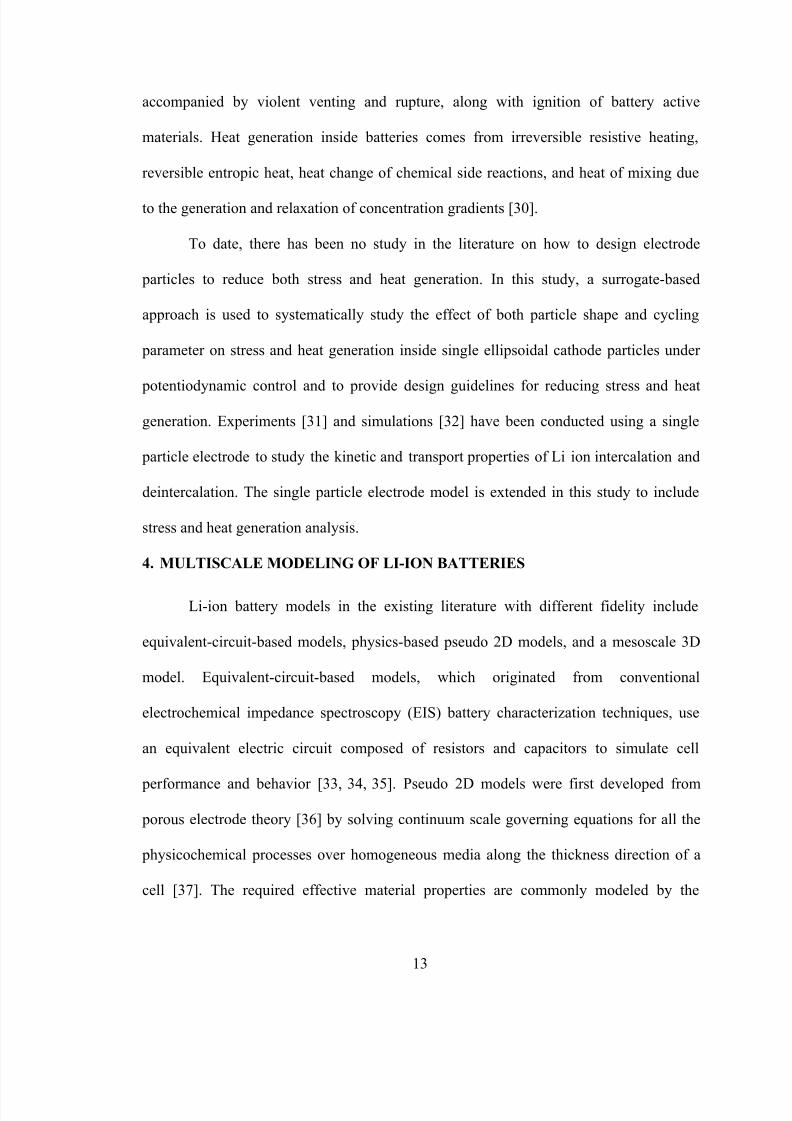
Commonly used design of experiments approaches include face centered central-
composite design (FCCD) [65], Latin hypercube sampling (LHS) [66], and orthogonal
arrays [67]. FCCD includes designs on 2 v vertices, 2 N v axial points (where N v is the
dimension of the design space) and N c repetitions of the central point. Rrepetitions at the
center reduce the variance and improve stability. An illustration for FCCD in three
dimensional design space is shown in Figure 1.5 (b). FCCD is not practical for higher
dimensional spaces ( N v > 8) because the number of simulations or experiments needed
becomes very high. LHS is a stratified sampling approach with the restriction that each of
the input variables has all portions of its distribution represented by input values. A
sample of size N s can be constructed by dividing the range of each input variable into N s
strata of equal marginal probability 1/ N s and sampling once from each stratum. Figure
1.5 (c) shows an example of LHS design for N s=6 points in a two dimensional design
space.
The obtained simulations or experiment results on the sampling points are used to
construct surrogate models; sampling points from the design of experiments for surrogate
model construction are sometimes also referred to as training points. Commonly used
surrogate models include polynomial response surface (PRS), kriging [68], radial basis
neural network (RBNN). Polynomial response surface represent the objective function as
8/21/2019 zhangxc_1
http://slidepdf.com/reader/full/zhangxc1 39/178
(a) Design of experiments
Numerical simulations or
experimental measurements at
sampling points
Construction of surrogate
models (Model selection and
Refining design
space or adding
more sampling
points, if necessary
Model Validation
(b) (c)
Figure 1.5: Surrogate modeling: (a) key steps of surrogatemodeling; (b) design of experiments by FCCD; (c) design of
experiments by LHS.
22

8/21/2019 zhangxc_1
http://slidepdf.com/reader/full/zhangxc1 40/178
23
a linear combination of monomial basis functions. An example for the second order
polynomial response surface approximation is
0
1 1
ˆ ( )v v N N
i i ij i j
i i j i
f x x x β β β
= = ≤
= + +
∑ ∑∑x , (10)
where the coefficients β are determined by minimizing the approximation error in a least
square sense. The kriging model estimates the value of a function (response) at some
unsampled location as the sum of two components: the linear model (e.g. polynomial
trend)1
( )i i
i
p
f β =
∑ x and a systematic departure Z (x) representing low (large scale) and high
frequency (small scale) variation components, respectively. The systematic departure
components are assumed to be correlated as a function of distance between the locations
under consideration. Gaussian function is commonly used for the correlation,
( ) ( )2
1
exp( ), ( ), ( )x s θi i i
i
v N
C Z Z x sθ =
= − −∏ . (11)
Optimal parametersi
θ are determined for maximum likelihood estimation. The RBNN
model uses linear weighted combinations of radially symmetric functions ( )ia x based on
Euclidean distance or other such metrics to approximate response functions. A typical
radial function is the Gaussian function,
( )2
( ) radbas , where radbas( ) na b n e−= − =x s x . (12)
Parameter b in the above equation is inversely related to a user-defined parameter ‘spread
constant’ that controls the response of the radial basis function. Typically, spread
constant is selected between zero and one. A very high spread constant would result in a
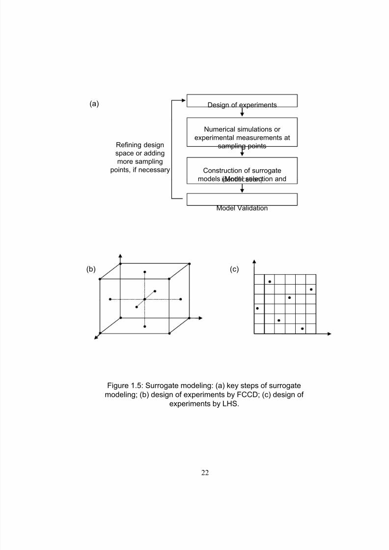
highly non-linear response function. An example of surrogate models (PRS, kriging and

8/21/2019 zhangxc_1
http://slidepdf.com/reader/full/zhangxc1 41/178
24
RBNN) constructed based on training data of 5 sampling points obtained from the
analytical functions y=exp( x4) is shown in Figure 1.6.
After surrogate models are constructed, their accuracy is evaluated using error
measures. Error in approximation of surrogate models at any given point x is defined as
the difference between the actual function ( ) y x and the predicted response ˆ( ) y x .
However, the actual response in the design space is unknown. We can not compute the
actual errors of surrogate model prediction. Therefore, error measures are practically
obtained on the available training data used for surrogate model construction or
additional testing data obtained from numerical simulations or experimental
measurements. Commonly used error measures based on the available training data
include the adjusted coefficient of multiple determination 2adj R for polynomial response
surface and prediction error sum of squares (PRESS) [69]. The coefficient of multiple
determination is defined as
2
1 E
T
SS
R SS = − , (13)
where2
1
ˆ s N
E i i
i
SS y y
∑ is the sum of square of residuals and2
1
s N
T i
i
SS y y
∑ is the
total sum of squares (1
1 s N
i
s i
y y N
∑ ). This coefficient can be interpreted as the proportion
of response variation explained by the surrogate model (PRS). 2 1 R = indicates that the
fitted model explains all variability in y. However, this coefficient increases weakly with
the number of terms used in PRS. Therefore, it is important to take into account the
number of terms used in the regression mode, which results in the definition for the
adjusted coefficient of multiple determination 2adj R . 2
adj R is defined as
8/21/2019 zhangxc_1
http://slidepdf.com/reader/full/zhangxc1 42/178
Figure 1.6: An example of varies surrogate models constructed based
on training data obtained from the analytical function y =exp( x 4).
25
8/21/2019 zhangxc_1
http://slidepdf.com/reader/full/zhangxc1 43/178
26
( )
( )
( )
( ) ( )2 2
adj
11 1 1
1
E s s
T s s
SS N p N R R
SS N N p
− −= − = − −
− −, (14)
where p is the number of terms used in polynomial response surface model. The adjusted
coefficient increases only if the newly added term improves the model. For a good fit,
this coefficient should be close to one. PRESS is a cross-validation error. It is the
summation of squares of all PRESS residues, each of which is calculated as the
difference between the simulation by computer experiments and the prediction by
surrogate models constructed from the remaining sampling points while excluding the
point of interest [69]. PRESS RMS (root mean square) is the root mean square of the
PRESS residues,
( ) 2
1
1ˆPRESS RMS ( )
si
i i
i s
N
y y N
−
=
= −∑ , (15)
where N s is the number of training points, i y is the value of the objective function
obtained from numerical simulations or experimental measurements at training point i,
and ( )ˆ i
i y − is the prediction by the surrogate model constructed by leaving point i out and
using the remaining N s−1 training points. This strategy is also called leave-one-out. The
smaller the PRESS RMS, the more accurate the surrogate model will be. PRESS RMS is
expensive to calculate using leave-one-out strategy for larger number of training points
since N s different surrogate models need to be constructed based N s different sets of
training data containing N s−1 points. To solve this problem, a k -fold strategy was used to
approximate PRESS RMS [70, 71]. In this approach, the available data ( p points) are first
divided into p/k clusters. Each fold is constructed using a point randomly selected from

8/21/2019 zhangxc_1
http://slidepdf.com/reader/full/zhangxc1 44/178
27
each of the clusters. Out of the k folds, a single fold is retained as the validation data for
testing the model, and the remaining k-1 folds are used as training data. k -fold turns out to
be the leave-one-out when k=p. This k -fold strategy provides a much faster approach for
calculating PRESS. Surrogate models are also evaluated by comparing surrogate model
prediction and actual numerical simulation or experimental measurement results on
testing points. The actual root mean square error could be approximated by using the
prediction error on testing points as
test2
1test
1ˆRMSE ( )i i
i
N
y N =
= −∑ , (16)
where i y is the actual data from numerical simulation or experimental measurements at
testing points i, and ˆi is the prediction by surrogate models at testing points i. With the
calculated error measures for surrogate models constructed, one can try to select the best
surrogate model based on a given error measure as the criterion. However, since the
actual response of the objective function is unknown, one does not really know which
error measure criterion performs the best. Sometimes, it can be risky to use individual
surrogate models for predicting objective functions. Weighted average surrogates or
ensemble of surrogates was proposed to provide more robust prediction of objective
functions than individual surrogates [72]. Surrogate models validated to have adequate
accuracy can be used for further analysis such as global sensitivity analysis and
optimization of objective functions. If the desired accuracy is not achieved, another
iteration of the surrogate modeling process should be repeated with refined design space
or additional sampling points in the same design space.

8/21/2019 zhangxc_1
http://slidepdf.com/reader/full/zhangxc1 45/178
28
With the constructed surrogate models, global sensitivity analysis can be
conducted to study the importance of design variables. Global sensitivity analysis
quantifies the variation of the objective functions caused by design variables. The
importance of design variables is presented by main factor and total effect indices [57].
Main factor is the fraction of the total variance of the objective function contributed by a
particular variable in isolation, while the total effect includes contribution of all partial
variances in which the variable of interest is involved. When Sobol’s method [73] is
commonly used to calculate global sensitivity indices, a surrogate model f (x) of a square
integrable objective as a function of a vector of independent input variables x in domain
[0, 1] is decomposed as the sum of functions of increasing dimensionality as
( ) ( ) ( ) ( )0 12 1 2, , , ,i i ij i j N N i i j
f f f x f x x f x x x<
= + + + +∑ ∑x…
… . (17)
In the context of global sensitivity analysis, the total variance denoted as V ( f ) can be
shown to be equal to
( )1...
1 1 ,
...v
vv
i iji i j
N
N
V f V V V = ≤ ≤
= + + +∑ ∑ . (18)
Each of the terms V i , V ij , V ijk ⋅⋅⋅ represents the partial contribution or partial variance of
the independent variables or set of variables to the total variance and provides an
indication of their relative importance. The main factor index of variable xi is defined as
main
( )
i
i
V
S V f = . (19)
The total effect index of variable xi is defined as

8/21/2019 zhangxc_1
http://slidepdf.com/reader/full/zhangxc1 46/178
29
, , ,total
...
( )
i ij ijk
j j i j j i k k i
i
V V V
S V f
≠ ≠ ≠
+ + +
=∑ ∑ ∑
. (20)
Constructed surrogate models can also be used for objective function
optimization. With the objective function globally mapped over the design space by
surrogate models, global minima or maxima of the objective function can be identified
for the single objective optimization. For two-objective optimization, a pareto front can
be generated using surrogate models constructed to identify the trade-offs between two
objective functions.
6. SCOPE AND OUTLINE OF THE DISSERTATION
In Chapter 2, an intercalation-induced stress model with the analogy to thermal
stress modeling is developed to determine localized intercalation-induced stress in
electrode particles. Intercalation-induced stress is calculated within ellipsoidal electrode
particles with a constant diffusion flux assumed at the particle surface. In Chapter 3,
surrogate-based analysis is conducted to systematically investigate the effect of both
particle shape and cycling parameter on stress and heat generation inside single
ellipsoidal cathode particles under potentiodynamic control. The diffusion flux on the
particles is determined by the rate of electrochemical reactions modeled by the Butler-
Volmer equation. The outcome from this surrogate-based analysis provides guidelines for
electrode particle design that will reduce stress and heat generation during battery
cycling. Chapters 2 and 3 facilitate the understanding of physicochemical mechanisms by
choosing a simple geometry, single electrode particles, without dealing with geometric
complexity. Chapter 4 develops a battery scale model that takes into account the
complicated 3D microstructure information of battery electrode materials. A multiscale

8/21/2019 zhangxc_1
http://slidepdf.com/reader/full/zhangxc1 47/178
30
modeling framework is proposed to deal with the disparate length scales present in Li-ion
cells. Closure terms from macroscopic scale governing equations are extracted from
microscopic scale modeling of electrode particle clusters. Scale bridging is achieved by
serial coupling using a surrogate-based approach.
BIBLIOGRAPHY
1. U.S. Environmental Protection Agency, Greenhouse Gas Emissions from the U.S.
Transportation Sector, 1990-2003, www.epa.gov/otaq/climate.htm, accessed June
6, 2006.
2. C. Samaras, and K. Meisterling, Life Cycle Assessment of Greenhouse Gas
Emissions from Plug-in Hybrid Vehicles: Implications for Policy, Environmental
Science & Technology, 42, 3170–3176 (2008).
3. D. Linden and T. B. Reddy (editors), Handbook of Batteries (third edition),
McGraw-Hill, 2002.
4. Official web page of the United States Advanced Battery Consortium (USABC),
http://www.uscar.org/guest/view_team.php?teams_id=12, accessed June 6, 2009.
5. H. Li, X. Huang, L. Chen, Z. Wu, and Y. Liang, A High Capacity Nano-Si
Composite Anode Material for Lithium Rechargeable Batteries, Electrochemicaland Solid-State Letters, 2(11), 547-549 (1999).
6. C. K. Chan, H. Peng, G. Liu, K. MclLwrath, X. F. Zhang, R. A. Huggins and Y.
Cui, High-Performance Lithium Battery Anodes Using Silicon Nanowires, Nature
Nanotechnology, 3(1), 31-35 (2008).
7. T. Ohzuku, A. Ueda, and N. Yamamoto, Zero-Strain Insertion Material of
Li[Li1/3Ti5/3]O4 for Rechargeable Lithium Cells, Journal of the Electrochemical
Society, 142(5), 1431-1435 (1995).
8. R. J. Gummow, A. de Kock, and M. M. Thackeray, Improved Capacity Retentionin Rechargeable 4V Lithium/Lithium Manganese Oxide (Spinel) Cells, Solid
State ionics, 69, 59-67 (1994).
9. A. K. Padhi, K. S. Nanjundaswamy, and J. B. Goodenough, Phospho-olivines asPositive-Electrode Materials for Rechargeable Lithium Batteries, Journal of the
Electrochemical Society, 144(4), 1188-1194 (1997).

8/21/2019 zhangxc_1
http://slidepdf.com/reader/full/zhangxc1 48/178
31
10. T. Ohzuku and Y. Makimura, Layered Lithium Insertion Material of
LiCo1/3Ni1/3Mn1/3O2 for Lithium-Ion Batteries, Chemistry Letters, 7, 642-643
(2001).
11. N. Ravet, Y. Chouinard, J. F. Magnan, S. Besner, M. Gauthier, and M. Armand,
Electroactivity of Natural and Synthetic Triphylite, Journal of Power Sources, 97-
98, 503-507 (2001).
12. H. Joachin, T. D. Kaun, K. Zaghib, and J. Prakash, Electrochemical and Thermal
Studies of Carbon-Coated LiFePO4 Cathode, Journal of The ElectrochemicalSociety, 156 (6), A401-A406 (2009).
13. S.-Y. Chung, J. T. Bloking and Y.-M. Chiang, Electronically Conductive
Phospho-Olivines as Lithium Storage Electrodes, Nature Materials, 1, 123-128
(2002).
14. P. B. Balbuena and Y. Wang (editors), Lithium-Ion Batteries; Solid-ElectrolyteInterphase, Imperial College Press, London, 2004.
15. R. Spotnitz and J. Franklin, Abuse Behavior of High-Power, Lithium-Ion Cells,
Journal of Power SOurnces, 113, 81-100 (2003).
16. S. Leroy, F. Blanchard, R. Dedryvere, H. Martinez, B. Carre, D. Lemordant, and
D. Gonbeau, Surface Film Formation on a Grahite Electrode in Li-Ion Batteries:
AFM and XPS Study, Surface and Interface Analysis, 37, 773-781 (2005).
17. M. Itagaki, N. Kobari, S. Yotsuda, K. Watanabe, S. Kinoshita, and M. Ue, In Situ
Electrochemical Impedance Spectroscopy to Investigate Negative Electrode of
Lithium-Ion Rechargeable Batteries, Journal of Power Sources, 135, 255-261(2004).
18. J. Li and J. R. Dahn, An In Situ X-Ray Diffraction Study of the Reaction of Liwith Crystalline Si, Journal of The Electrochemical Society, 154(3), A156-A161
(2007).
19. X. Q. Yang, X. Sun, S. J. Lee, J. McBreen, S. Mukerjee, M. L. Daroux, and X. K.King, In Situ Synchrontron X-Ray Diffraction Studies of the Phase Transitions in
LixMn2O4 Cathode Materials, Electrochemical and Solid-State Letters, 2(4),
157-160 (1999).
20. M. Broussely, S. Herreyre, P. Biensan, P. Kasztejna, K. Nechev, and R. J.
Staniewicz, Aging Mechanism in Li Ion Cells and Calendar Life Predictions,
Journal of Power Sources 97-98, 13-21 (2001).
21. E. P. Roth and D. H. Doughty, Thermal Abuse Performance of High-Power
18650 Li-Ion Cells, Journal of Power Sources 128, 308-318 (2004).

8/21/2019 zhangxc_1
http://slidepdf.com/reader/full/zhangxc1 49/178
32
22. T. F. Fuller, M. Doyle, and J. Newman, Simulation and Optimization of the Dual
Lithium Ion Insertion Cell, Journal of the Electrochemical Society, 141(1), 1-10
(1994).
23. L. Song and J. W. Evans, Electrochemical-Thermal Modeling of Lithium Polymer
Batteries, Journal of The Electrochemical Society, 147(6), 2086-2095 (2000).
24. D. Wang, X. Wu, Z. Wang, and L. Chen, Cracking Causing Cyclic Instabilit of
LiFePO4 Cathode Material, Journal of Power Sources, 140, 125-128 (2005).
25. M.-R. Lim, W.-I. Cho, and K.-B. Kim, Preparation and Characterization of Gold-
Codeposited LiMn2O4 Electrodes, Journal of Power Sources 92, 168-176 (2001).
26. H. Wang, Y.-I. Jang, B. Huang, D. R. Sadoway, and Y.-M. Chiang, TEM Study
of Electrochemical Cycling-Induced Damage and Disorder in LiCoO2 Cathodesfor Rechargeable Lithium Batteries, Journal of the Electrochemical Society,
146(2), 473-480 (1999).
27. K. E. Aifantis and J. P. Dempsey, Stable crack growth in nanostructured Li-
batteries, Journal of Power Sources, 143, 203–211 (2005).
28. J. Christensen and J. Newman, Stress Generation and Fracture in Lithium
Insertion Materials, Journal of Solid State Electrochemistry, 10, 293–319 (2006).
29. S. Prussin, Generation and Distribution of Dislocations by Solute Diffusion,
Journal of Applied Physics, 32(10), 1876-1881 (1961).
30. K. E. Thomas, and J. Newman, Thermal Modeling of Porous Insertion Electrodes,
Journal of the Electrochemical Society, 150, A176-A192 (2003).
31. I. Uchida, H. Fujiyoshi, and S. Waki, Microvoltammetric Studies on SingleParticles of Battery Active Materials, Journal of Power Sources, 68, 139-144
(1997).
32. D. Zhang, B. N. Popov, and R. E. White, Modeling Lithium Intercalation of aSingle Spinel Particle under Potentiodynamic Control, Journal of The
Electrochemical Society, 147, 831-838 (2000).
33. M. W. Verbrugge and R. S. Conell, Electrochemical and Thermal
Characterization of Battery Modules Commensurate with Electric Vehicle
Integration, Journal of The Electrochemical Society, 149, A45-A53 (2002).
34. B. Y. Liaw, G. Nagasubramanian, R. G. Jungst, and D. H. Doughty, Modeling of
Lithium Ion Cells – A Simple Equivalent-Circuit Model Approach, Solid State
Ionics, 175, 835-839 (2004).
35. P. L. Moss, G. Au, E. J. Plichta, and J. P. Zheng, An Electrical Circuit for
Modeling the Dynamic Response of Li-Ion Polymer Batteries, Journal of The
Electrochemical Society, 155, A986-A994 (2008).

8/21/2019 zhangxc_1
http://slidepdf.com/reader/full/zhangxc1 50/178
33
36. J. Newman and W. Tiedemann, Porous-Electrode Theory with Battery
Applications, AIChE Journal, 21, 25-41 (1975).
37. M. Doyle, T. F. Fuller, and J. Newman, Modeling of Galvanostatic Charge andDischarge of the Lithium Polymer Insertion Cell, Journal of The Electrochemical
Society, 140, 1526-1533 (1993) .
38. C.-W. Wang and A. M. Sastry, Mesoscale Modeling of a Li-Ion Polymer Cell,
Journal of The Electrochemical Society, 154, A1035-A1047 (2007).
39. W. Shyy et al., Computational Technques for Complex Transport Phenomena,
Cambridge, 1997.
40. U. Hornung (editor), Homogenization and Porous Media, Springer, New York,
1997.
41. E. Sanchez-Palencia, Non-Homogeneous Media and Vibration Theory, edited byJ. Ehlers et al, Lecture Notes in Physics, Springer-Verlag, New York, 1980.
42. K. Matous, H. M. Inglis, X. Gu, D. Rypl, T. L. Jackson, and P. H. Geubelle,
Multiscale Modeling of Solid Propellants: from Particle Packing to Failure,
Composites Science and Technology, 67, 1694-1708 (2007).
43. S. Ghosh, K. Lee and P. Raghavan, A Multi-level Computational Model for
Multi-scale Damage Analysis in Composite and Porous Materials, International
Journal of Solids and Structures 38, 2335-2385 (2001).
44. C. C. Mei, Method of Homogenization Applied to Dispersion in Porous Media,
Transport in Porous Media 9: 261-274 (1992).
45. I. Lunati, S. Attinger, and W. Kinzelbach, Macrodispersivity for Transport inArbitrary Nonuniform Flow Fields: Asymptotic and Preasymptotic Results, Water
Resources Research 38 (10): Art. No. 1187 OCT 2002.
46. A. R. Martin, C. Saltiel, W. Shyy, Heat Transfer Enhancement with Porous
Inserts in Recirculating Flows, Journal of Heat Transfer, 120, 458-467 (1998).
47. E. Sozer and W. Shyy, Multi-scale Thermo-fluid Transport in Porous Media,
International Journal of Numerical Methods for Heat & Fluid Flow, 18(7/8) 883-
899 (2008).
48. J. G. Berryman and S. R. Pride, Volume Averaging, Effective Stress Rules, and
Inversion for Microstructural Response of Multicomponent Porous Media, Int. J.
Solids Structures, 35, 4811-4843 (1998).
49. M. Doyle, T. F. Fuller, and J. Newman, Modeling of Galvanostatic Charge and
Discharge of the Lithium Polymer Insertion Cell, Journal of The Electrochemical
Society, 140, 1526-1533 (1993) .
8/21/2019 zhangxc_1
http://slidepdf.com/reader/full/zhangxc1 51/178
34
50. P. D. Vidts and R. E. White, Governing Equations for Transport in Porous
Electrodes, Journal of The Electrochemical Society, 144, 1343-1353 (1997).
51. W. B. Gu, C. Y. Wang, and B. Y. Liaw, Micro-Macroscopic Coupled Modelingof Batteries and Fuel Cells, Journal of the Electrochemical Society, 145, 3407-
3418 (1998).
52. R. J. M. Smit, W. A. M. Brekelmans, and H. E. H. Meijer, Prediction of the
Mechanical Behavior of Nonlinear Heterogeneous Systems by Multi-Level Finite
Element Modeling, Computer Methods in Applied Mechanics and Engineering,155, 181-192 (1998).
53. V. Kouznetsova, W. A. M. Brekelmans, and F. P. T. Baaijens, An Approach to
Micro-Macro Modeling of Heterogeneous Materials, Computational Mechanics
27, 37-48 (2001).
54. W. E, B. Engquist, X. Li, W. Ren, and E. Vanden-Eijnden, HeterogeneousMultiscale Methods: a Review, Communications in Computational Physics, 2,
367-450 (2007).
55. L. Tan and N. Zabaras, Multiscale Modeling of Alloy Solidification Using a
Database Approach, Journal of Computational Physics 227, 728–754 (2007).
56. O. Rohrle, J. B. Davidson, and A. J. Pullan, Bridging Scales: A Three-Dimensional Electromechanical Finite Element Model of Skeletal Muscle, SIAM
Journal on Scientific Computing, 30, 2882–2904 (2008).
57. N. V. Queipo, R. T. Haftka, W. Shyy, T. Goel, R. Vaidyanathan, and P. K.
Tucker, Surrogate-based Analysis and Optimization, Progress in AerospaceSciences, 41, 1-28 (2005).
58. T. Goel, S. Thakur, R. T. Haftka, W. Shyy, and J. Zhao, Surrogate model-basedstrategy for cryogenic cavitation model validation and sensitivity evaluation,
International Journal of Numerical Methods in Fluids, 58, 969-1007 (2008).
59. A. Samad, K.-Y. Kim, T. Goel, R. T. Haftka, and W. Shyy, Multiple SurrogateModeling for Axial Compressor Blade Shape Optimization, Journal of Propulsion
and Power, 24 (2), 302-310 (2008).
60. B. D. Marjavaara, T. S. Lundstrom, T. Goel, Y. Mack, and W. Shyy, Hydraulic
Turbine Diffuser Shape Optimization by Multiple Surrogate Model
Approximations of Pareto Fronts, 129, 1228-1240 (2007).
61. Y.-C. Cho, B. Jayaraman, F. A. C. Viana, R. T. Haftka, and W. Shyy, Surrogate
Modeling for Characterizing the Performance of Dielectric Barrier Discharge
Plasma Actuator, 46th AIAA Aerospace Sciences Meeting and Exhibit, January 7-
10, 2008, Reno, Nevada.

8/21/2019 zhangxc_1
http://slidepdf.com/reader/full/zhangxc1 52/178
35
62. P. Trizila, C.-K. Kang, M. Visbal, and W. Shyy, A Surrogate Model Approach in
2D versus 3D Flapping Wing Aerodynamic Analysis, 12th
AIAA/iSSMO
Multidisciplinary Analysis and Optimization Conference, Spetember 10-12,
2008, Victoria, British Columbia, Canada.
63. J. I. Madsen, W. Shyy and R. T. Haftka, Response Surface Techniques for
Diffuser Shape Optimization, AIAA Journal, 38, 1512-1518 (2000).
64. T. Goel, R. Vaidyanathan, R. T. Haftka, W. Shyy, N. V. Queipo, and K. Tucker,
Response Surface Approximation of Pareto Optimal Front in Multi-ObjectiveOptimization, Computer Methods in Applied Mechanics and Engineering, 196,
879–893 (2007).
65. G. E. P. Box and K. B. Wilson, On the Experimental Attainment of OptimumConditions, Journal of the Royal Statistical Society, Series B (Methodological),
13, pp. 1-45 (1951).
66. M. D. McKay and R. J. Beckman and W. J. Conover, A Comparison of Three
Methods for Selecting Values of Input Variables in the Analysis of Output from aComputer Code, Technometrics, 21, 239-245 (1979).
67. A. Hedayat, N. Sloane, and J. Stufken, Orthogonal Arrays: Theory and
Applications, Springer, Series in Statistics, Berlin: Springer, 1999.
68. G. Matheron, Principles of Geostatistics, Economic Geology, 58:1246–66 (1963).
69. R. H. Myers, and D. C. Montgomery, Response Surface Methodology: Processand Product Optimization Using Designed Experiments, pp. 17-48, John Wiley &
Sons Inc: New York, 1995.
70. R. Kohavi, A Study of Cross-Validation and Bootstrap for Accuracy Estimationand Model Selection, “Proceedings of the Fourteenth International Joint
Conference on Artificial Intelligence, 2, 1137-1143 (1995).
71. F. A. C. Viana, R. T. Haftka, and V. Steffen, Multiple Surrogates: How Cross-Validation Errors Can Help Us to Obtain the Best Predictor, Structural and
Multidisciplinary Optimization, In Press, DOI 10.1007/s00158-008-0338-0.
72. T. Geol, R. T. Haftka, W. Shyy and N. V. Queipo, Ensemble of Surrogates,
Structural and Multidisciplinary Optimization, 33(3), 199-216 (2007).
73. I. M. Sobol, Sensitivity Analysis for Nonlinear Mathematical Models.Mathematical Modeling and Computational Experiment, 1(4), 407–414 (1993).

8/21/2019 zhangxc_1
http://slidepdf.com/reader/full/zhangxc1 53/178
36
CHAPTER II
NUMERICAL SIMULATION OF INTERCALATION-INDUCED STRESS IN LI-
ION BATTERY ELECTRODE PARTICLES*
1. INTRODUCTION
Severe, particle-level strains induced during both production and cycling have
been putatively linked to lifetime limiting damage in lithium-ion cells. Intercalation and
deintercalation of Li ions into cathodic lattices, including LiCoO2 [1], LiMn2O4 [2] and
LiFePO4 [3], have been postulated to result in fraction inside the particles, as determined
by experimentation on model systems. In LiMn2O4 for example, 6.5% percent of volume
change has been reported when Mn2O4 is lithiated into LiMn2O4 [4]. The simulation of
LiMn2O4 indicated that intercalation-induced stress could exceed the ultimate strength of
the material [5]. Also, stress generation due to cell-scale loads by compression during
manufacturing has been shown to result in localized particle stresses that are much higher
in the graphite anode material [6] (the ratio between local and global stresses is around 25
to 140). Indeed, stresses of these orders exceed known strength of the materials which
comprise the most commonly used, and most promising, cathode materials (Table 2.1 [4,
7, 8, 9]).
* The material in this chapter is a published paper: X. Zhang, W. Shyy, and A. M. Sastry,
Numerical Simulation of Intercalation-Induced Stress in Li-Ion Battery Electrode
Particles, Journal of the Electrochemical Society, 154(10) A910-A916 (2007).

8/21/2019 zhangxc_1
http://slidepdf.com/reader/full/zhangxc1 54/178
.
t e r c a l a t i o n p r o c e s s
m a t e r i a l s i n t h e i n
d s t r a i n
i n c a t h o d
a b l e 2 . 1 : S t r e s s a
37

8/21/2019 zhangxc_1
http://slidepdf.com/reader/full/zhangxc1 55/178
38
Stress generation due to Li-intercalation, and more generally in other processes, has been
modeled in prior work at the particle scale. Christensen and Newman estimated stress
generation in the lithium insertion process in carbon anode [10] and LiMn2O4 cathode [5]
particles. More broadly, stresses induced by species diffusion have been studied in other
fields including metal oxidation and semiconductor doping. Prussin [11] first treated
diffusion induced stress by analogy to thermal stress. In this study, stress generation
during doping of boron and phosphorus into silicon wafer was studied. Li [12] studied
diffusion-induced stress or chemical stress in elastic media of simple geometries
following this method, as well. Yang [13] studied the evolution of chemical stress in a
thin plate by considering the interaction between chemical stress and diffusion Prussin’s
thermal stress analogy [11].
Though these sets of efforts offer a means of stress estimation at the particle scale,
by different physical assumptions, the implementations to date have not been applied to
the problem of three-dimensional stresses. Because of the presently unknown
contributions of manufacturing- and intercalation-induced stresses in Li-cells, this
correlation is critical: in determining optimal materials and manufacturing methods for
these cells. Both global and localized loads must be estimated, in order to select materials
able to resist fracture. Further, the role of localized particle fracture in capacity fade has
been implied, but not quantified, given the general lack of understanding of localized
loads in batteries.
Thus, the present work is focused on determining localized particle stresses in
cathodic particles. Here we select the LiMn2O4 system following [14, 15, 16, 17, 18] on
battery performance modeling, [19, 20] on atomic scale simulation of structure and

8/21/2019 zhangxc_1
http://slidepdf.com/reader/full/zhangxc1 56/178
39
diffusion properties, and [5] on intercalation-induced stress simulation because of the low
cost and environmental safety of LiMn2O4. We have the following objectives in this
study:
1) To determine diffusion-induced stresses according to an analogy to
thermal stress, following [11, 12 and 13] for single particles, and
determine the correspondence with prior work in Li cells [5];
2) To verify the implementation of a single-particle model numerically,
using a finite difference scheme and reproduction of simple results; and
3)
To implement this model into a full finite element scheme, and simulate
stresses induced by intercalation in particles of nonspherical geometry.
2. METHODS
2.1 Stress-Strain Relations
For intercalation processes, the lattice constants of the material may be assumed to
change linearly [4] with the volume of ions inserted, which results in stresses. Therefore,
one can calculate intercalation-induced stress by analogy to thermal stress. Prussin [11]
previously treated concentration gradients analogously to those generated by temperature
gradients in an otherwise unstressed body.
Stress-strain relations including thermal effects are written classically for an elastic
body [21], as
ε xx − α T =1
E σ xx − ν σ yy + σ zz ( )[ ] (1a)
ε yy − α T =1
E σ yy − ν σ xx + σ zz ( )[ ] (1b)

8/21/2019 zhangxc_1
http://slidepdf.com/reader/full/zhangxc1 57/178
40
ε zz − α T =1
E σ zz − ν σ xx + σ yy( )[ ] (1c)
ε xy = σ xy
2G, ε yz =
σ yz
2G, ε xz =
σ xz
2G (1d)
where ijε are strain components, ijσ are stress components, E is Young’s modulus, ν is
Poisson’s ratio, G is modulus of elasticity in shear, α is thermal expansion coefficient,
and T is the temperature change from the original value. Analogously, the stress-strain
relation with the existing of concentration gradients can be written as [13]
( )[ ]ijijkk ijij
c
E δ δ νσ σ ν ε
3
~1
1 Ω+−+= (2)
where 0~ ccc −= is the concentration change of the diffusion species from the original
(stress-free) value, and Ω is partial molar volume of solute. Eq. (2) can be rewritten to
obtain the expression for the components of stresses,
( ) ijkk ijij c δ β λε με σ ~2 −+= (3)
where ( )ν += 12 E , ( )ν ν λ 212 −= , and ( ) 323λ β +Ω= . As usual in elasticity,
the strain tensor is related to displacement u as [21]
⎟⎟ ⎠
⎞⎜⎜⎝
⎛
∂
∂+
∂
∂=
i
j
j
i
ij x
u
x
u
2
1ε (4)
and the equilibrium equation, neglecting body forces, is [21]
)3,2,1(0, == jiijσ (5)
Substitution of Eq. (3) and (4) into (5), leads to the displacement equations [22]
∇2ui + λ + μ ( )uk ,ki − β ?c,i = 0 (i =1, 2, 3). (6)
The boundary condition for the case of a single particle is that the particle surface is
traction-free. This condition can be expressed as [22]

8/21/2019 zhangxc_1
http://slidepdf.com/reader/full/zhangxc1 58/178
41
0=++= nml p zx yx xxnx σ σ σ (7a)
0=++= nml p zy yy xyny σ σ σ (7b)
0=++= nml p zz yz xz nz
σ σ σ (7c)
where nml ,, denote the direction cosines between the external normal and each axis.
Substitution of Eq. (3) and (4) into boundary conditions (7), yields
μ ui, j + u j,i( )n j + λ uk ,k − β c( )ni = 0 i =1, 2, 3 (8)
where l n =1 , mn =2 and nn =3 . Therefore, we are left to solve Eq. (6), with boundary
condition (8).
2.2 Diffusion Equation
As shown in Eq. (2) and (3), concentrations are needed to calculate intercalation-
induced stresses. To obtain a concentration profile, the insertion and extraction of ions
are modeled as a diffusion process. The effect of existing electrons in the solid on the
species flux of lithium can be neglected, because electrons are much more mobile than
intercalated atoms [23]. The chemical potential gradient is the driving force for the
movement of lithium ions. The velocity of lithium ions can be expressed as
∇−= M v (9)
where is the mobility of lithium ions and μ is the chemical potential. The species flux
can then be written as [23]
∇−== MccvJ (10)
where c is the concentration of the diffusion component (lithium ions).
The electrochemical potential in an ideal solid solution can be expressed as [13,
24]

8/21/2019 zhangxc_1
http://slidepdf.com/reader/full/zhangxc1 59/178
42
h X RT σ Ω−+= ln0 (11)
where 0 is a constant, R is gas constant, T is absolute temperature, X is the molar
fraction of lithium ion, Ω is partial molar volume of lithium ion, and hσ is the
hydrostatic stress, which is defined as ( ) 3/332211 σ σ σ σ ++=h (where ijσ are the
elements in stress tensor). Eq. (10) and (11) show that the diffusion flux depends on
concentration, temperature, and stress field. Substitution of (11) into (10), assuming
temperature is uniform, and noting that
( ) cc
RT X X
RT X RT ∇=∇=∇11
ln , (12)
an expression of species flux (when there is no temperature gradient inside the particle)
can be obtained as
⎟ ⎠
⎞⎜⎝
⎛ ∇Ω
−∇−= h RT
cc D σ J (13)
where RT D = is the diffusion coefficient. Conservation of species gives
0=⋅∇+∂∂
Jt
c. (14)
Then, substituting Eq. (13) into (14) gives, finally,
⎟ ⎠
⎞⎜⎝
⎛ ∇Ω
−∇⋅∇Ω
−∇=∂∂
hh RT
cc
RT c D
t
cσ σ 22 , (15)
as the governing equation for the diffusion process. The initial condition is 0cc = , with
the boundary condition
J = − D ∇c − Ωc
RT ∇σ h
⎝⎜
⎠⎟ =
in
F (16)

8/21/2019 zhangxc_1
http://slidepdf.com/reader/full/zhangxc1 60/178
43
where ni is the current density on the particle surface (which is assumed to be a constant,
known value in this study), and F is Faraday’s constant.
2.3 Numerical Methods
a. Finite Difference Method for 1-D Problem
For the case of a spherical particle, the above equations become one-dimensional.
The stress tensor contains two independent components, radial stress r σ and tangential
stress t σ . The equilibrium equation (refer to Eq. (5)) for this case is simply
( ) 02
d
d =−+ t r r
r r σ σ
σ , (17)
and the stress-strain relations (referring to Eq. (2)) are
( ) c E
t r r ~
32
1 Ω+−= νσ σ ε (18)
( )[ ] c E
t r t t ~
3
1 Ω++−= σ σ ν σ ε . (19)
The strain-displacement relations (referring to Eq. (4)) are
r
ur
d
d=ε ,
r
ut =ε , (20)
and displacement equation (refer to Eq. (6)) is
r
c
r
u
r
u
r r
u
d
~d
31
12
d
d2
d
d22
2 Ω−+
=−+ν
ν . (21)
Integration of this equation yields a solution for u , from which stresses may be obtained.
Noting that stresses are finite at the center of the sphere ( 0=r ), and that radial stresses
are zero, 0=r σ , at the particle surface ( 0r r = ), the two constants in the solution can be
determined, as

8/21/2019 zhangxc_1
http://slidepdf.com/reader/full/zhangxc1 61/178
44
( ) ⎟⎟ ⎠
⎞⎜⎜⎝
⎛ −
−Ω
= ∫∫ r r cr
r r cr
E r r
r d~1d~1
13
2
0
2
3
0
2
3
0
0
ν σ , and (22)
( ) ⎟
⎟
⎠
⎞
⎜
⎜
⎝
⎛ −+
−
Ω=
∫∫cr r c
r r r c
r
E r r
t
~d~1d~2
13 0
2
30
2
30
0
ν σ . (23)
Eq. (22) shows that radial stress actually depends upon the difference between the global
and local averages of concentration.
The diffusion equation is (referring to Eq. (15)),
⎥⎥⎦
⎤
⎢⎢⎣
⎡⎟⎟ ⎠
⎞⎜⎜⎝
⎛
∂
∂+
∂
∂Ω−
∂
∂
∂∂Ω
−∂∂
+∂∂
=∂∂
r r r RT
c
r r
c
RT r
c
r r
c D
t
c hhh σ σ σ 222
2
2
2
. (24)
Eqs. (22) (23) allow calculation of hydrostatic stress, as
( )( ) ⎟
⎟ ⎠
⎞⎜⎜⎝
⎛ −
−Ω
=+= ∫ cr r cr
E r
t r h~d~3
19
23/2
0
0
2
3
0ν
σ σ σ . (25)
By assuming that the characteristic time for elastic deformation of solids is much smaller
than that for atomic diffusion, the elastic deformation can be treated as quasistatic [13].
Therefore, Eq. (25) can be substituted into Eq. (24) to obtain
⎥⎥⎦
⎤
⎢⎢⎣
⎡⎟⎟ ⎠
⎞⎜⎜⎝
⎛
∂∂
+∂∂
+⎟ ⎠
⎞⎜⎝
⎛ ∂∂
+∂∂
+∂∂
=∂∂
r
c
r r
cc
r
c
r
c
r r
c D
t
c 222
22
2
2
θ θ (26)
where( )ν
θ −
ΩΩ=
19
2 E
RT .
Substituting (25) into boundary conditions (16), one has
( ) F
i
r
cc D n=
∂∂
+−= θ 1J at 0r r = (27)
In this way, the two variables, concentration and stress, are decoupled.

8/21/2019 zhangxc_1
http://slidepdf.com/reader/full/zhangxc1 62/178
45
To solve the above equation numerically, it, along with boundary and initial
condition, is transformed into dimensionless form first, as
⎟⎟ ⎠
⎞
⎜⎜⎝
⎛
∂
∂+
∂
∂+
⎟ ⎠
⎞
⎜⎝
⎛
∂
∂+
∂
∂+
∂
∂=
∂
∂
r
c
r r
cc
r
c
r
c
r r
c
t
c
ˆ
ˆ
ˆ
2
ˆ
ˆˆˆ
ˆ
ˆˆ
ˆ
ˆ2
ˆ
ˆ
ˆ
ˆ
2
22
2
2
θ θ (28)
1ˆ0 ≤≤ r , T t ˆˆ0 ≤≤ (where T satisfies ) 1ˆˆ,1ˆˆ === T t r c )
1ˆ =r , ( ) I r
cc =
∂∂
+−ˆ
ˆˆˆ1 θ ; 0ˆ =r , 0
ˆ
ˆ=
∂∂r
c
max0 /ˆ,0ˆ ccct ==
where dimensionless variables are defined as
0
ˆr
r r =
2
0
ˆr
tDt =
max
ˆc
cc = max
ˆ cθ θ = F Dc
r i I n
max
0=
In the above equations, maxc is the stoichiometric maximum concentration and 0c is the
initial concentration. It may be seen that the effect of discharge current density, particle
radius and diffusion coefficient are all combined into the dimensionless current density
I .
The numerical procedure is as follows. For each time step, concentration
distribution is solved first by Eq. (28). Then, the concentration is substituted into Eq. (22)
(23) to calculate stresses. Eq. (28) is a nonlinear, parabolic partial differential equation.
The finite difference method is used here to solve the equation.
First Eq. (28) is rewritten as
2
2
ˆˆ ˆ ˆ ˆ ˆ2 2ˆ ˆˆ(1 )ˆ ˆ ˆ ˆ ˆˆ
c c c c cc
t r r r r r
θ θ θ
⎛ ⎞∂ ∂ ∂ ∂= + + + +⎜ ⎟⎜ ⎟∂ ∂ ∂∂ ⎝ ⎠
. (29)

8/21/2019 zhangxc_1
http://slidepdf.com/reader/full/zhangxc1 63/178
46
To discretize the differential equation into difference equations, the problem is linearized
by taking the value from the previous time step for the terms in the two parentheses on
the right hand side. The Crank-Nicolson method is used for other terms. The difference
equation obtained is
( ) ( )( )
( ) ( )( )r
ccccc
r r
cc
r
r
ccccccc
t
cc
n
i
n
i
n
i
n
in
i
i
n
i
n
i
i
n
i
n
i
n
i
n
i
n
i
n
in
i
n
i
n
i
ˆ22
ˆˆˆˆˆˆ
ˆ
2
ˆ2
ˆˆˆˆ
21
ˆ2
ˆ2ˆˆˆ2ˆˆ)ˆˆ1(
ˆ
ˆˆ
11
1
1
1
111
2
11
11
1
1
1
1
Δ
−+−⎟⎟ ⎠
⎞⎜⎜⎝
⎛ +
Δ
−+++
Δ
−++−++=
Δ
−
−++
−+
+−+
−+++
−+
++
θ θ
θ
(30)
Terms including r /1 will be singular at the particle center 0ˆ =r . To solve this difficulty,
noting that
0ˆ
ˆ=
∂∂r
c when 0ˆ =r (31)
L’Hopital’s rule can be used
2
2
0ˆ ˆ
ˆ
ˆ
ˆ
ˆ
1lim
r
c
r
c
r r ∂∂
=∂∂
→
(32)
to eliminate the r /1 factor. Thus, Eq. (28) becomes
2
2
ˆ ˆ ˆ ˆˆ ˆˆ(3 3 )ˆ ˆ ˆˆ
c c c cc
t r r r θ θ
∂ ∂ ∂ ∂⎛ ⎞= + + ⎜ ⎟∂ ∂ ∂∂ ⎝ ⎠, (33)
which has no singularity at 0ˆ =r . Therefore, Equation (33) will be solved at 0ˆ =r while
Equation (29) is solved elsewhere.
At two boundary points, imaginary points (out of the boundary) are used to
discretize the governing equation; the concentration values of these imaginary points are
obtained by central differencing of the flux boundary condition at the boundary points.

8/21/2019 zhangxc_1
http://slidepdf.com/reader/full/zhangxc1 64/178
47
The Thomas algorithm is used to solve the tridiagonal system of the difference
equations. The simulation is halted when the concentration on the particle surface 1ˆ =r
reaches the stoichiometric maximum.
b. Finite Element Method for 3-D Problem
The three-dimensional problem was simulated using FEMLAB (COMSOL
Multiphysics®
). Two models are included in the multiphysics simulation, PDE (partial
differential equation) model (general form) and solid stress-strain model. In PDE model,
the diffusion process is described by the generalized form of PDE
0=Γ⋅∇+∂∂
t
c (34)
where
⎟ ⎠
⎞⎜⎝
⎛ ∇Ω
−∇−=Γ h RT
cc D σ . (35)
In the solid stress-strain model, ‘thermal expansion’ is included as a load based on the
variable of concentration c instead of temperature in thermal stress calculations.
2.4 Material Properties
All the material properties used in the simulation for Mn2O4 are listed in Table 2.2
[5, 25]. From Eq. (2), we see that that partial molar volume plays a role analogous to a
thermal expansion coefficient, in calculating intercalation-induced stress. To obtain the
value for this property, the volume change of 6.5% for 2.0= y to 995.0= y of LiyMn2O4
is used [5]. The volume change of 6.5%, giving a strain of 0.0212, corresponds to the
concentration change from 2.0= y to 995.0= y . Therefore, by noting the analogy
between thermal expansion coefficient and 3/Ω , partial molar volume is

8/21/2019 zhangxc_1
http://slidepdf.com/reader/full/zhangxc1 65/178
.
r o p e r t i e s o f M n 2 O
a b l e 2 . 2 : M a t e r i a l
48
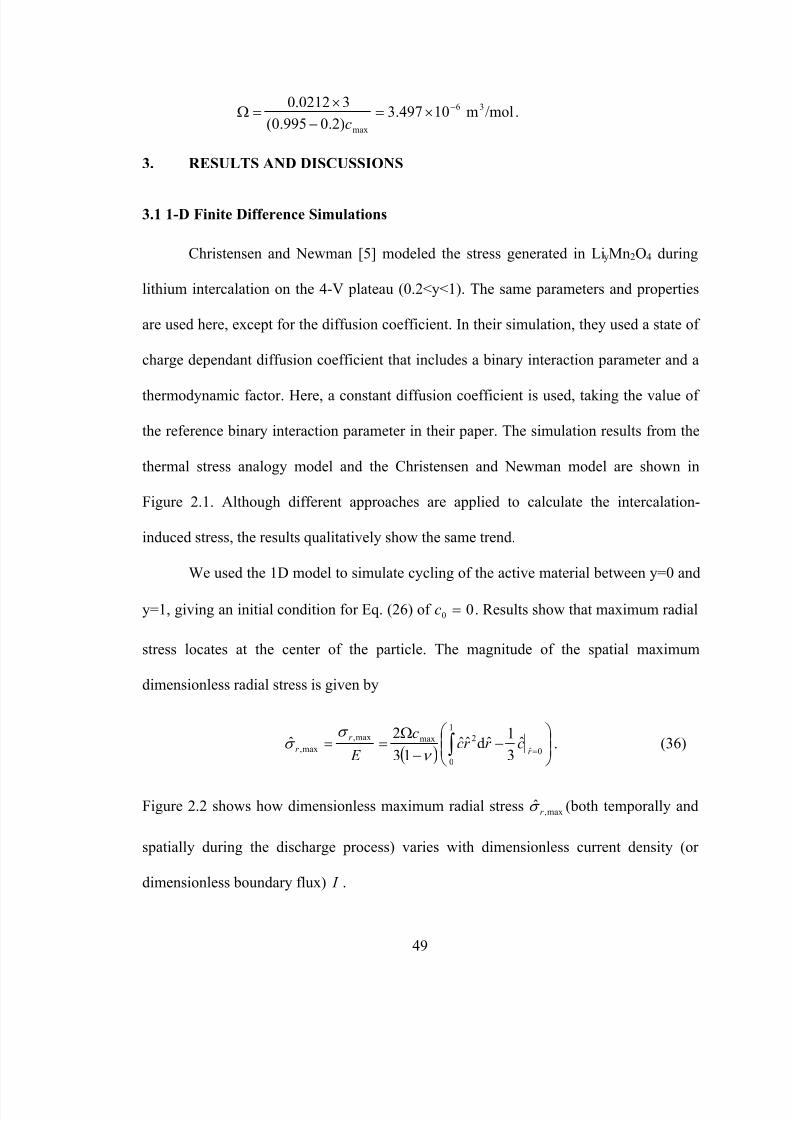
8/21/2019 zhangxc_1
http://slidepdf.com/reader/full/zhangxc1 66/178
49
/molm10497.3)2.0995.0(
30212.0 36
max
−×=−
×=Ω
c.
3. RESULTS AND DISCUSSIONS
3.1 1-D Finite Difference Simulations
Christensen and Newman [5] modeled the stress generated in LiyMn2O4 during
lithium intercalation on the 4-V plateau (0.2<y<1). The same parameters and properties
are used here, except for the diffusion coefficient. In their simulation, they used a state of
charge dependant diffusion coefficient that includes a binary interaction parameter and a
thermodynamic factor. Here, a constant diffusion coefficient is used, taking the value of
the reference binary interaction parameter in their paper. The simulation results from the
thermal stress analogy model and the Christensen and Newman model are shown in
Figure 2.1. Although different approaches are applied to calculate the intercalation-
induced stress, the results qualitatively show the same trend.
We used the 1D model to simulate cycling of the active material between y=0 and
y=1, giving an initial condition for Eq. (26) of 00 =c . Results show that maximum radial
stress locates at the center of the particle. The magnitude of the spatial maximum
dimensionless radial stress is given by
( ) ⎟⎟ ⎠
⎞⎜⎜⎝
⎛ −
−
Ω==
=∫ 0ˆ
1
0
2maxmax,
max,ˆ
3
1ˆdˆˆ
13
2ˆ
r
r
r cr r cc
E ν
σ σ . (36)
Figure 2.2 shows how dimensionless maximum radial stress max,ˆ
r σ (both temporally and
spatially during the discharge process) varies with dimensionless current density (or
dimensionless boundary flux) I .

8/21/2019 zhangxc_1
http://slidepdf.com/reader/full/zhangxc1 67/178
Figure 2.1: Comparison of simulation results of two models.
50

8/21/2019 zhangxc_1
http://slidepdf.com/reader/full/zhangxc1 68/178
Figure 2.2: Maximum dimensionless radial stress versus
dimensionless current density.
51

8/21/2019 zhangxc_1
http://slidepdf.com/reader/full/zhangxc1 69/178
52
As shown in Figure 2.2, maximum radial stress (spatially and temporally) inside
an electrode particle during the discharge process increases with increasing dimensionless
current density when 7.20 << I . However, maximum radial stress decreases with
increasing dimensionless current density when it is larger than 2.7. The decrease of stress
occurs because the concentration profile is not fully developed, so that the global average
term (first term in the parenthesis) in Eq. (36) decreases with dimensionless current
density, while the local average (second term in the parenthesis) remains constant. This is
not desirable in the cycling of batteries, because it reduces material utilization. Therefore,
only the increasing branch of the curve is actually feasible. The increasing branch shows
that increase of discharge current density and particle radius will increase the
intercalation-induced stress. In other words, smaller particles should be used to reduce
intercalation-induced stresses.
As mentioned earlier, the model used here to simulate the intercalation-induced
stress is a diffusion-stress coupling model. The effect of stress on diffusion will be
discussed briefly using the one-dimensional equations for a spherical particle.
Substituting Eq. (25) into (13), we obtain
( )r
cc D
∂∂
+−= θ 1J . (37)
In Eq. (37), cθ is always a positive number, and the effective diffusion coefficient is
essentially ( ) Dc D >+θ 1 . Therefore, the diffusion is enhanced due to the extra term cθ ,
which basically comes from hydrostatic stress gradient term in Eq. (13). In other words,
stress enhances the diffusion. This stress enhancement effect is also demonstrated
numerically, as shown in Figure 2.3. It shows the concentration profile at t=1000s with
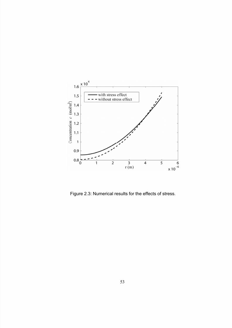
8/21/2019 zhangxc_1
http://slidepdf.com/reader/full/zhangxc1 70/178
Figure 2.3: Numerical results for the effects of stress.
53

8/21/2019 zhangxc_1
http://slidepdf.com/reader/full/zhangxc1 71/178
54
discharge current density 2mA2=i on the surface. The profile including the effect of
stress has a smaller gradient than that excluding the stress effect, confirming that stress
enhances diffusion.
Substituting the material properties into the expression of ( )[ ] RT E ν θ −Ω= 192 2 ,
we obtain /molm101.557 3-5×=θ . If the maximum concentration is used, 356.0max =cθ ,
which is not negligible compared to unity. Therefore, for the case of LiMn2O4, the stress
effect cannot be neglected. From the expression for θ , it can be observed that θ has
smaller magnitude when the material has smaller modulus E and smaller partial molar
volume Ω . Thus, the stress effect on diffusion may be negligible when the material is
soft (i.e. having a low modulus).
3.2 3-D Finite Element Simulation Results
The 1-D finite difference simulation, with 4001 grid points and a time step of
0.001s, was used as the reference solution to study the convergence of finite element
method. Figure 2.4 shows the 2-norm errors (differences) between the finite element
solutions and finite difference reference solutions at t=1000s. The parameters used in the
simulations are current density 2mA2=i , and particle radius m50 =r . The finite
element solutions converged to the reference solution as the number of elements used
increased. At the same time, Figure 2.4 also shows that solutions from 1-D finite
difference method and 3-D finite element method were consistent, because the
nondimensionalized errors of concentration and stress from 17359 elements simulation
were 7105.6 −× and 5105.1
−× respectively (if nondimensionalized by the maximum values
at t=1000s inside the particle).
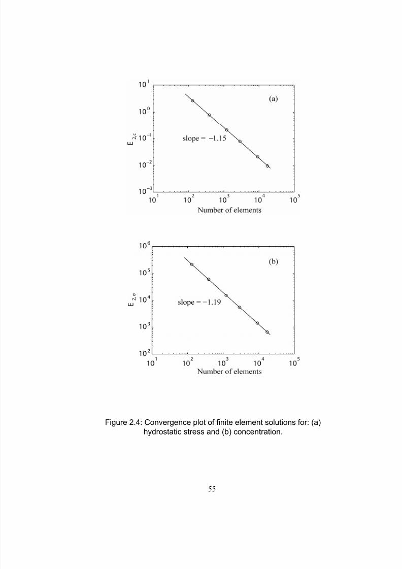
8/21/2019 zhangxc_1
http://slidepdf.com/reader/full/zhangxc1 72/178
Figure 2.4: Convergence plot of finite element solutions for: (a)
hydrostatic stress and (b) concentration.
55

8/21/2019 zhangxc_1
http://slidepdf.com/reader/full/zhangxc1 73/178
56
To study the effect of aspect ratios on the intercalation-induced stress, ellipsoids
with different aspect ratios were studied. The current density on the surface is fixed at
2mA2=i . For the ellipsoid, the lengths of three semi-axes a , b and c satisfy ba = ,
and the aspect ratio is defined as ac /=α , as sketched in Figure 2.5. The volumes of the
ellipsoids were fixed, at V = 4π × 53 3 m3 . A set of simulations, with different aspect
ratios, were run by FEMLAB.
Characteristic solution profiles of concentration, von Mises stress and shear stress
yz σ are shown in Figure 2.6 at the end of the discharge process (when the surface
concentration reaches the stoichiometric maximum) for an ellipsoid with aspect ratio
1.953. Figure 2.6 shows that 1) the concentration is higher around the poles; 2) the von
Mises stress is larger around the equator; and 3) shear stress has its maximum on the
surface. The solution profiles have the same patterns for other ellipsoids with different
aspect ratios.
Figure 2.7 shows how the maximum von Mises stress inside the particle varies
during the discharge process for particles with different aspect ratios. It takes less time
for particles with larger aspect ratios to completely discharge. Also, during discharge,
von Mises stress increases first, and then drops. In Figure 2.7, it can be observed that
when aspect ratio increases, the stress increases first (for aspect ratios from 1.0 to 1.37)
and then decreases (for aspect ratios from 1.37 to 3.81). For ellipsoids with aspect ratio
2.92 and 3.81, the intercalation-induced stress is smaller than that inside a sphere (aspect
ratio 1.0).
Figure 2.8 shows how aspect ratio affects (a) peak value of maximum von Mises
stress, and (b) peak value of maximum shear when the volumes of particles are fixed.
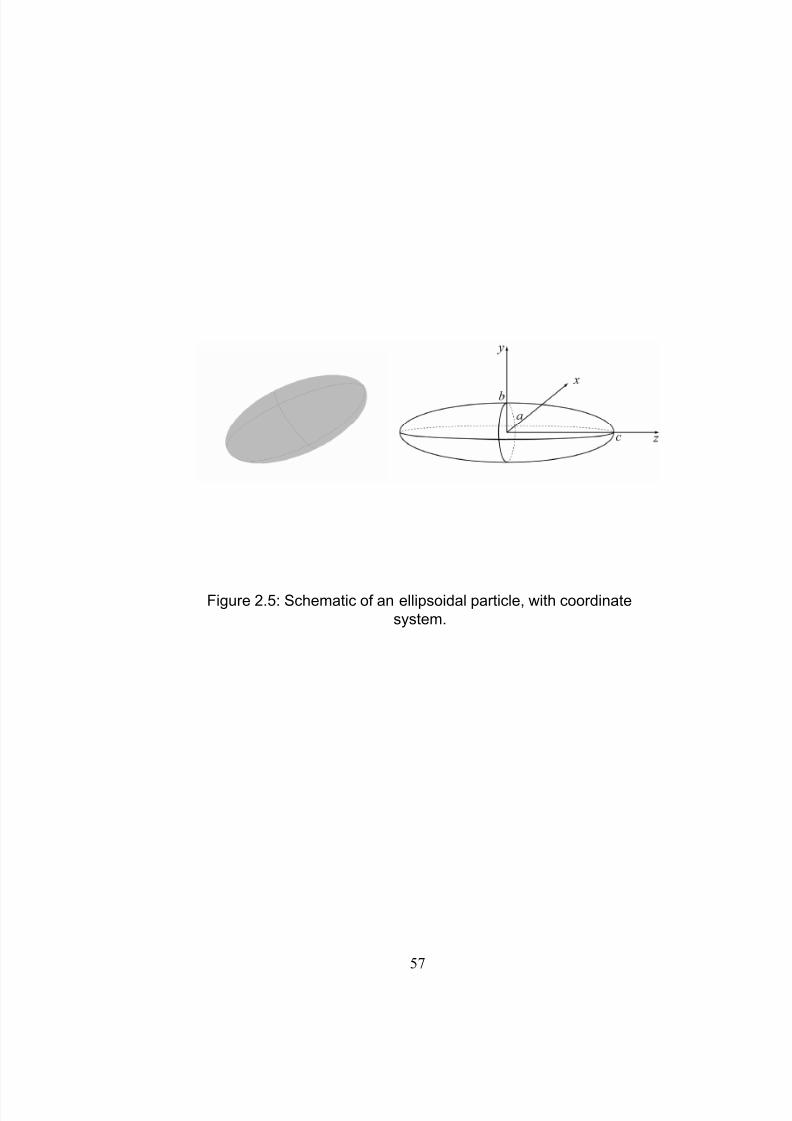
8/21/2019 zhangxc_1
http://slidepdf.com/reader/full/zhangxc1 74/178
Figure 2.5: Schematic of an ellipsoidal particle, with coordinate
system.
57

8/21/2019 zhangxc_1
http://slidepdf.com/reader/full/zhangxc1 75/178
Figure 2.6: Solutions at the end of discharge for an ellipsoid of aspect
ratio 1.953, (a) concentration, (b) von Mises stress, and (c) shear
s ress.
58

8/21/2019 zhangxc_1
http://slidepdf.com/reader/full/zhangxc1 76/178
Figure 2.7: Maximum von Mises stress during discharge, for various
ellipsoids.
59

8/21/2019 zhangxc_1
http://slidepdf.com/reader/full/zhangxc1 77/178
Figure 2.8: The effect of aspect ratio, for fixed particle volume.
60

8/21/2019 zhangxc_1
http://slidepdf.com/reader/full/zhangxc1 78/178
61
Figure 2.8 (a) shows that the peak value of maximum von Mises stress inside the particle
increases first and then decreases as the aspect ratio increases. Once the aspect ratios are
larger than 2.2, the maximum von Mises stress is less than that inside spherical particles
(aspect ratio 1). Figure 2.8 (b) shows that peak value of maximum shear stress decreases
as aspect ratio increases. The results of Figure 2.8 show that particles with larger aspect
ratios have less intercalation-induced stress generation, when the particle volume is
preserved.
The peak values of maximum von Mises stresses are shown in Figure 2.8 (a).
Maximum stress first increases, then decreases with aspect ratio. This is due to two
competing effects. When particle volume is preserved, increased aspect ratios result in
increase of the longer semi-axis c, and reduction of shorter, semi-axes a and b.
Elongation of the longer semi-axis tends to increase maximum stress, while reduction of
the shorter semi-axes tends to decrease the maximum stress. This competition results in a
global maximum of stress at an aspect ratio of ~1.37.
To further illustrate the effect of semi-axes on maximum stress, an additional set
of simulations were performed, in which the shorter semi-axes a and b were fixed, and
aspect ratio α was increased by elongation of the longer semi-axis, c. Results, obtained
with a discharge current density 2mA2=i , are shown in Figure 2.9. Stress first
increases with aspect ratio because of the increase of longer semi-axis, and then decreases
slightly until asymptotically approaching the cylinder/fiber limit, i.e. α∞. As
represented by the dashed line in Figure 2.9, no physically relevant solutions are obtained
for α>7.9, because the discharge process stops when the concentration on the particle
surface reaches stoichiometric maximum, before the maximum stress actually

8/21/2019 zhangxc_1
http://slidepdf.com/reader/full/zhangxc1 79/178
Figure 2.9: The effect of aspect ratio, for fixed shorter semi axes.
62

8/21/2019 zhangxc_1
http://slidepdf.com/reader/full/zhangxc1 80/178
63
reaches the peak value. To quantitatively illustrate this point, for an ellipsoid with aspect
ratio 10, the stress reaches its peak value at t = 721s. However, the simulation should
terminate at t = 617.5s, when the surface concentration already reaches stoichiometric
maximum. The maximum stress at t = 721s is 52.47MPa, and the stress at t = 617.5s is
52.26MPa. Therefore, the stress when the process is terminated, is only slightly smaller
than the peak value.
4. CONCLUSION
Intercalation-induced stresses during the discharge process were simulated in this
study using a stress-diffusion coupling model. Intercalation-induced stresses were
simulated by analogy to thermal stress. Simulations of spherical particles show that larger
particle sizes and larger discharge current densities give larger intercalation-induced
stresses. Furthermore, internal stress gradients significantly enhance diffusion.
Simulation results for ellipsoidal particles show that large aspect ratios are preferred, to
reduce the intercalation-induced stresses. In total, these results suggest that it is desirable
to synthesize electrode particles with smaller sizes and larger aspect ratios, to reduce
intercalation-induced stress during cycling of lithium-ion batteries.
8/21/2019 zhangxc_1
http://slidepdf.com/reader/full/zhangxc1 81/178
64
BIBLIOGRAPHY
1. H. Wang, Y.-I Jang, B. Huang, D. R. Sadoway, and Y.-M. Chiang, TEM Study of
Electrochemical Cycling-Induced Damage and Disorder in LiCoO2 Cathodes for
Rechargeable Lithium Batteries, Journal of the Electrochemical Society, 146 (2),473-480 (1999).
2. M.-R. Lim, W.-I. Cho, and K.-B. Kim, Preparation and characterization of gold-
codeposited LiMn2O4 electrodes, Journal of Power Sources, 92, 168-176 (2001).
3. D. Wang, X. Wu, Z. Wang, and L. Chen, Cracking Causing Cyclic Instability of
LiFePO4 Cathode Material, Journal of Power Sources, 140, 125–128 (2005).
4. W. I. F. David, M. M. Thackeray, L. A. de Picciotto, and J. B. Goodenough,
Structure Refinement of the Spinel-Related Phases Li2Mn2O4 And Li0.2Mn2O4,
Journal of Solid State Chemistry, 67 (2), 316-323 (1987).
5. J. Christensen and J. Newman, A Mathematical Model of Stress Generation and
Fracture in Lithium Manganese oxide, Journal of the Electrochemical Society,
153 (6), A1019-A1030 (2006).
6. Y.-B. Yi, C.-W. Wang, and A. M. Sastry, Compression of Packed Particulate
Systems: Simulation and Experiments in Graphite Li-ion Anodes, Journal of
Engineering Materials and Technology, vol. 128, 73-80 (2006).
7. S. Pyun, J. Go, and T. Jang, An Investigation of Intercalation-Induced Stresses
Generated During Lithium Transport Through Li1- CoO2 Film Electrode Using a
Laser Beam Deflection Method, Electrochimica Acta, 49 4477–4486 (2004).
8. Y. Kim, S. Pyun, and J. Go, An Investigation of Intercalation-Induced Stresses
Generated During Lithium Transport Through So-Gel Derived LixMn2O4 Film
Electrode Using a Laser Beam Deflection Method , Electrochimica Acta, 51, 441–
449 (2005).
9. A. K. Padhi, K. S. Nanjundaswamy, and J. B. Goodenough, Phospho-olivines as
Positive-Electrode Materials for Rechargeable Lithium Batteries, Journal of the
Electrochemical Society, 144 (4), 1188-1194 (1997).
10. J. Christensen and J. Newman, Stress Generation and Fracture in Lithium
Insertion Materials, Journal of Solid State Electrochemistry, 10 (5), 293-319(2006).
11. S. Prussin, Generation and Distribution of Dislocations by Solute Diffusion,
Journal of Applied Physics, 32(10), 1876-1881 (1961).
12. J. C. M. Li, Physical Chemistry of Some Microstructural Phenomena,
Metallurgical Transactions A, 9A, 1353-1380 (1978).

8/21/2019 zhangxc_1
http://slidepdf.com/reader/full/zhangxc1 82/178
65
13. F. Yang, Interaction between Diffusion and Chemical Stresses, Materials Science
and Engineering A, 409, 153–159 (2005).
14. M. Doyle, J. Newman, and A. S. Gozdz, C. M. Schmutz, and J.-M. Tarascon,
Comparison of Modeling Predictions with experimental Data from PlasticLithium Ion Cells, Journal of the Electrochemical Society, 143(6), 1890-1903
(1996).
15. R. Darling and J. Newman, Modeling a Porous Intercalation Electrode with Two
Characteristic Particle Sizes, Journal of the Electrochemical Society, 144(12),
4201-4208 (1997).
16. P. Arora, M. Doyle, A. S. Gozdz, R. E. White, and J. Newman, Comparison
between Computer Simulations and Experimental Data for High-Rate Discharges
of Plastic Lithium-Ion Batteries, Journal of Power Sources, 88, 219–231 (2000).
17. E. Deiss, D. Haringer, P. Novak, and O. Haas, Modeling of The Charge– Discharge Dynamics of Lithium Manganese Oxide Electrodes for Lithium-Ion
Batteries, Electrochimica Acta, 46, 4185–4196 (2001).
18. R. Darling and J. Newman, Modeling Side Reactions in Composite LiMn2O4
Electrode, Journal of the Electrochemical Society, 145(3), 990-998 (1998).
19. C. Y. Ouyang, S. Q. Shi, Z. X. Wang, H. Li, X. J. Huang and L. Q. Chen, Ab
Initio Molecular-Dynamics Studies on LixMn2O4 as Cathode Material For
Lithium Secondary Batteries, Europhysics Letters, 67 (1), 28–34 (2004).
20. B. Ammundsen, J Roziere, and M. S. Islam, Atomistic Simulation Studies of
Lithium and Proton Insertion in Spinel Lithium Manganates, The Journal of Physical Chemistry. B 101, 8156-8163 (1997).
21. S. P. Timoshenko and J. N. Goodier, Theory of Elasticity, McGraw-Hill, New
York, (1970).
22. N. Noda, R. B. Hetnarski, and Y. Tanigawa, Thermal Stresses (second edition),
Taylor & Francis, New York (2003).
23. W. R. McKinnon and R. R. Haering, Physical Mechanisms of Intercalation. In
Modern Aspects of Electrochemistry, No. 15, edited by Ralph E. White et al.
Plenum Press, New York (1983).
24. W. L. Wang, S. Lee, and J. R. Chen, Effect Of Chemical Stress On Diffusion in a
Hollow Cylinder, Journal of Applied Physics, 91(12), 9584-9590 (2002).
25. A. Paolone, R. Cantelli, G. Rousse, and C. Masquelier, The Charge Order
Transition and Elastic/Anelastic Properties of LiMn2O4, Journal of Physics:
Condensed Matter , 15, 457-465 (2003).

8/21/2019 zhangxc_1
http://slidepdf.com/reader/full/zhangxc1 83/178
66
CHAPTER III
SURROGATE-BASED ANALYSIS OF STRESS AND HEAT GENERATION
WITHIN SINGLE CATHODE PARTICLES UNDER POTENTIODYNAMIC
CONTROL*
1. INTRODUCTION
Excessive heat generation in Li batteries, resulting in thermal runaway, results in
complete cell failure accompanied by violent venting and rupture, along with ignition of
battery active materials [1, 2, 3, 4]. Stress-induced fracture also putatively degrades
performance in these cells, as evidenced by observation of fractured surfaces in post
mortem analysis of batteries [5, 6, 7]. Stress generation results from lithium ion extraction
from the cathode (deintercalation), transport across the electrolyte and insertion into the
anode (intercalation), and the reverse reaction [8]. Intercalation-induced stress varies
cyclically, and thus damage aggregates with usage [5]. Particle-scale fracture of active
materials results in performance degradation of batteries due to the loss of electrical
contact and subsequent increase in the surface area subjected to side reactions [9]. These
phenomena, heat and stress generation, undoubtedly amplify one another, and both
phenomena are governed by cell kinetics. Inclusion of heat generation, mechanical
* The material in this chapter is a published paper: X. Zhang, A. M. Sastry and W. Shyy,
Intercalation-induced Stress and Heat Generation within Single Lithium-Ion Battery
Cathode Particles, Journal of the Electrochemical Society,155(7), A542-A552 (2008).

8/21/2019 zhangxc_1
http://slidepdf.com/reader/full/zhangxc1 84/178
67
stresses, and chemical kinetics in models at critical scales, i.e. particle scales, appears
necessary, and progress in each is discussed in order.
It is important to distinguish between heat transfer and heat generation analyses in
battery materials. We use “heat generation” to refer to the sources of heat in the cell;
“heat transfer”, by contrast, refers to the resulting distribution of temperature. Though the
sources of heat generation may be readily determined, solution for the distribution of
temperature requires even more detailed understanding of both geometry and materials
properties, as will be discussed later. Heat transfer analyses of Lithium-ion batteries have
stemmed from work on full cells [10]. This classic work [10] was later extended to
consider the effect of lithium concentration in intercalation compounds [1]. Foci of
subsequent studies have mainly been on improved modeling of heat transfer, rather than
refinement of geometric models to the particle scale. A three-dimensional (3D) model
was been developed, considering anisotropic conductivity, to simulate the temperature
distribution inside lithium polymer batteries under galvanostatic discharge for a dynamic
power profile [11]. Later, a layerwise 3D model (assuming different conductivities for
each homogeneous layer), was derived [12], in which radiation and convection were
considered.
Thus, progress to date in heat transfer modeling has been restricted to
consideration of continuum layers, though modeling at the particle scale appears
necessary at this time, given our ability to select particle geometry within electrodes.
Meanwhile, models have appeared in intercalation-induced stress which do address the
particle scale, e.g. a one-dimensional model to estimate stress generation within spherical
electrode particles [13 ] and a two-dimensional model to predict electrochemically
8/21/2019 zhangxc_1
http://slidepdf.com/reader/full/zhangxc1 85/178
68
induced stresses [14]. Neither, however, has considered complex particle shapes or the
effect of layerwise thickness on critical percolation limits [15]. In more recent work [16],
a three-dimensional model based on a thermal stress analogy has been used to simulate
the intercalation-induced stress inside cathode particles, but without consideration of
electrochemical kinetics.
In order to fully and predictively link thermal and stress-induced failures, kinetic
effects must also be understood, in tandem with detailed models of electrode architecture,
in three dimensions, and for complex particle shape. Though it has been established that
microscopic features of structures in batteries, including particle shape and size
distributions, are important factors in battery performance [17], models have not been
reported that incorporate electrochemical kinetics. Thus, in the present work, we model a
LiMn2O4 cathode particle under potentiodynamic control, with linearly variable applied
potential to the particle [18,19]. The cathode particle was assumed to be homogeneous.
We had the following specific objectives:
1) To develop and numerically implement particle scale models to simulate
intercalation-induced stress and heat generation, and to interrogate the interactions among
intercalation, stress and heat generation, for spherical particles;
2) To understand, using surrogate-based analysis, how stress and heat
generation depend upon the ratio of axial lengths for ellipsoidal cathode particles, and the
operating conditions (discharge time).
Our general methodology comprised two sequential efforts. First, we developed a
model that physically links intercalation-induced stress and thermal stress, following
prior work [16]. Three distinct sources of heat generation were considered, namely, heat

8/21/2019 zhangxc_1
http://slidepdf.com/reader/full/zhangxc1 86/178
69
of mixing, entropic heat, and resistive heating [1]. Though heat generation at this scale is
different, we do not at present have sufficient information on local heat transfer
coefficients within anisotropic particles to properly model heat transfer, and thus
determination of localized temperature distribution via heat transfer analysis is not
attempted here. Implementation of the model requires physical parameters, including
partial molar volume [16], Young’s modulus [16] and the derivative of open-circuit
potential (OCP) over temperature [20].
The second effort, in surrogate modeling, comprised use of surrogate models to
analyze relationships among stress and heat generation, and ellipsoidal particle
morphology and operating conditions. We first conducted simulations on selected
training points in critical regions, using the models developed to obtain the stress and
heat generation. The simulation results were then approximated by surrogate models
which were used, after validation, for further analysis of stress and heat generation for
different particle geometries and cycling rates.
2. ELECTROCHEMICAL, MECHANICAL AND THERMAL MODELING
In lithium-ion batteries, actual cathode particle morphology varies with synthesis
methods [21, 22, 23, 24]. Primary particles, made of crystalline grains, are agglomerated
using polymeric binders (e.g. poly (vinylidene fluoride) (PVdF) [2, 25]) and conductive
additives such as carbon black [25, 26], nonaqueous ultrafine carbon suspensions [27]
and graphite [28, 29] are incorporated to form secondary particles. Typical cathode
compositions and particle sizes are shown in Table 3.1 [Ref. 28, 25, 26, 22, 30, 31]. Sizes
range from 0.3 to 4 μm for primary particles, and 11 to 60 μm for secondary particles.
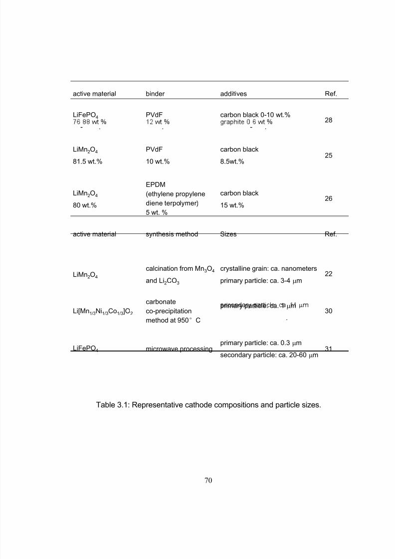
8/21/2019 zhangxc_1
http://slidepdf.com/reader/full/zhangxc1 87/178
active material binder additives Ref.
LiFePO4 PVdF carbon black 0-10 wt.%28
- . . - .
LiMn2O4
81.5 wt.%
PVdF
10 wt.%
carbon black
8.5wt.%25
EPDM
LiMn2O4
80 wt.%(ethylene propylenediene terpolymer)
5 wt. %
carbon black15 wt.%
26
active material synthesis method Sizes Ref.
LiMn2O4
calcination from Mn3O4
and Li2CO3
crystalline grain: ca. nanometers
primary particle: ca. 3-4 μm22
Li[Mn1/3Ni1/3Co1/3]O2
carbonate
co-precipitationprimary particle: ca. 1 μm
30
method at 950°C .
LiFePO4 microwave processingprimary particle: ca. 0.3 μm
secondary particle: ca. 20-60 μm31
Table 3.1: Representative cathode compositions and particle sizes.
70

8/21/2019 zhangxc_1
http://slidepdf.com/reader/full/zhangxc1 88/178
71
Modeling of these aggregates at the scale of single crystals requires molecular or
atomistic simulations. Thus, we restrict our considerations in the present study to a pure
active material (LiMn2O4) without inclusions. Our model cathodes particles are
homogeneous, isotropic single-phase ellipsoidal particles (prolate spheroids) or spherical
particles. The stress localization due to interaction between the crystalline grains is not
considered in stress generation simulations, and the temperature inside a particle is
assumed to be uniform in heat generation simulations.
Determination of intercalation-induced stress and heat generation first requires
mapping of concentration distribution and current density. Concentrations are obtained
by solving the diffusion equation with appropriate boundary conditions for each case (see
section 2.1.1). To model the intercalation-induced stress, a constitutive equation is used
to relate intercalation-induced strain. A heat generation model developed for a whole cell
[1] is used here, because our simulations rely on the assumption that the cathode particle
behaves as one electrode of a whole cell, incorporating experimental parameters from
microelectrode studies [18], wherein a single cathode electrode and the counter electrode
(lithium foil) comprise the electrochemical cell.
2.1 Model of Intercalation
An intercalation process can ideally be modeled as a diffusion process with
boundary flux determined by the electrochemical reaction rate. The model of the
intercalation process presented in this section includes a Li-ion transport equation and a
boundary condition determined by the electrochemical kinetics on the particle surface
under potentiodynamic control.

8/21/2019 zhangxc_1
http://slidepdf.com/reader/full/zhangxc1 89/178
72
2.1.1 Li-Ion Transport Equation
Li-ion diffusion is driven by the chemical potential gradient. For a given
concentration and stress gradients, the diffusion flux is given by [16]
⎟ ⎠
⎞⎜⎝
⎛ ∇
Ω−∇−= h
RT
cc D σ J , (1)
where c is the concentration of Li-ion, hσ is the hydrostatic stress, defined as
( ) 3/332211 σ σ σ σ ++=h (where
ijσ is the elements in stress tensor), D is the diffusion
coefficient, R is the general gas constant and T is temperature. With substitution of
Equation (1) into the mass conservation equation, we obtain the species transport
equation as follows [16],
0=⎥⎦
⎤⎢⎣
⎡⎟ ⎠
⎞⎜⎝
⎛ ∇
Ω−∇−⋅∇+
∂∂
h RT
cc D
t
cσ . (2)
The boundary condition for this equation is that the flux on the particle surface is
related to the discharge/charge current densityn
i as
F RT
cc D
n
h
i
J =⎟ ⎠
⎞⎜⎝
⎛ ∇
Ω−∇−= σ , (3)
where F is Faraday’s constant.
2.1.2 Electrochemical Kinetics under Potentiodynamic Control
The current density on the particle surface depends on the electrochemical
reaction rate. The reactions at the positive electrode are
LiMn2O4 ⇔ Li1- xMn2O4+ xLi++ xe
-
During charge, the positive electrode is oxidized, and lithium ions are extracted from the
positive electrode particle. During discharge, the positive electrode is reduced and lithium

8/21/2019 zhangxc_1
http://slidepdf.com/reader/full/zhangxc1 90/178
73
ions are inserted into the positive electrode particle. Chemical kinetics (reaction rate) are
described by the Butler-Volmer equation [32, 33], as
( )
⎭
⎬⎫
⎩
⎨⎧
⎥
⎦
⎤⎢
⎣
⎡−−⎥
⎦
⎤⎢
⎣
⎡ −== η
β η
β
RT
F
RT
F
F
i
F
i J n exp
1exp0 , (4)
where 0i is exchange current density, η is surface overpotential, and β is a symmetry
factor which represents the fraction of the applied potential that promotes the cathodic
reaction[33].
The exchange current density 0i is given by,
( ) ( ) ( ) β β
θ
β
sl ccc Fk i −−= 11
0 , (5)
where l c is the concentration of lithium ion in the electrolyte, sc is the concentration of
lithium ion on the surface of the solid electrode,θ c is the concentration of available
vacant sites on the surface ready for lithium intercalation (which is the difference
between stoichiometric maximum concentration and current concentration on the surface
of the electrode scc −max ), and k is a reaction rate constant[32].
In Equation (4), the surface overpotential is the difference between the potential
of the solid phase (compared to the electrolyte phase) V and the open circuit potential
(OCP) U [32]
U V −=η (6)
A fit of the experimental results [34] of OCP for LiMn2O4 is illustrated in Figure 3.1 (a).
OCP depends upon the state of charge y , i.e., the atomic ratio of lithium in the electrode
LiyMn2O4; this is a measure of the lithium concentration in the electrode. As shown in
Figure 3.1 (a), there are two plateaus in the potential distribution, resulting from the
ordering of the lithium ions on one half of the tetrahedral 8a sites of LiMn2O4 [35].

8/21/2019 zhangxc_1
http://slidepdf.com/reader/full/zhangxc1 91/178
Figure 3.1: Potentials: (a) OCP of LiMn2O4 and (b)applied potential
sweeping profile during one cycle.
74

8/21/2019 zhangxc_1
http://slidepdf.com/reader/full/zhangxc1 92/178
75
Following the numerical study [19], the potential of the solid phase is assumed, because
of the small size of particles, to be uniform within each particle, having the value of the
applied potential,
appU V = , (7)
when under microvoltammetric study (for example, [18]). This assumption of a uniform
potential distribution will be evaluated in Section 4. Under potentiodynamic control, the
applied potential changes linearly with time [18, 19] for fixed potential sweep rate v .
Once the applied potential reaches the upper bound, the potential sweep rate changes sign
to sweep backward. Figure 3.1(b) shows an example of the potential sweep, with
mV/s4.0=v . Increasing applied potential, in the first half cycle, drives the charging
process, while the decreasing applied potential, in the second half cycle, drives the
discharging process. As the potential cycles between 3.5102V and 4.3102V [19], the
electrode particle is thus charged and discharged.
For this applied potential stimulus, the initial condition for the species transport
equation (Equation (2)) is max00996.0 ccc
t ==
=.
2.1.3 Parameters and Material Properties
A reasonable way to obtain the lithium ion concentration in the electrolyte
l c would be to solve the species transport equation in the electrolyte. However, it is
assumed to be a constant value in this study following [19]. The values of parameters
and material properties used in this study (unless otherwise stated) are listed in Table 3.2.
2.2 Intercalation-Induced Stress Model
The constitutive equation between stress and strain, including the effect of
intercalation-induced stress by the analogy to thermal stress, is

8/21/2019 zhangxc_1
http://slidepdf.com/reader/full/zhangxc1 93/178
symbol value
β 0.5
c l 1000 mol/m3 [19]
c max 2.37×10⁴ mol/m3[19]
k 1.9×10⁻⁹ m5/2s-1mol-1/2 [19]
D 2.2×10⁻⁹ cm2/s [19]
V 0.4 mV/s
r 0 5 μm
Table 3.2: Parameters and material properties for the intercalation
model (where r 0 is the radius of a spherical particle).
76

8/21/2019 zhangxc_1
http://slidepdf.com/reader/full/zhangxc1 94/178
77
( )[ ] ijijkk ijij
c
E δ δ νσ σ ν ε
3
~1
1 Ω+−+= (8)
where ij
ε are strain components,ij
σ are stress components, E is Young’s modulus, ν is
Poisson’s ratio, 0
~ ccc −= is the concentration change of the diffusion species (lithium ion)
from the original (stress-free) value, and Ω is the partial molar volume of lithium [16].
Stress components are subjected to the force equilibrium equation
)3,2,1(0,
== jiij
σ . (9)
A Young’s modulus GPa10= E and a partial molar volume /molm10497.3 36−×=Ω [16] are
assumed here. Equation (2) and (8) are coupled through concentration c , and stresshσ .
2.3 Heat Generation Model
There are four sources of heat generation inside lithium ion batteries during
operation [1]
( ) ( )∫∑∑∑ ∂
∂
−+Δ+∂
∂
+−= vt
c
H H r H T
U
IT U V I Q g d j i
ijavg
ijijk
k
avg
k
avgavg
(10)
The first term, ( )avgU V I − , is the irreversible resistive heating, where I is the current of the
cell, V is the cell potential, and avgU is the volume averaged open circuit potential.
Resistive heating is caused by the deviation of the cell potential from its equilibrium
potential by resistance to the passage of current. The second term, T U IT ∂∂ avg , is the
reversible entropic heat, whereT
is temperature. The third term, ∑Δ
k k
avg
k r H
, is the heat
change of chemical side reactions, where avg
k H Δ is the enthalpy of reaction for chemical
reaction k , and k r is the rate of reaction k . The fourth term, ( )∫∑∑ ∂∂− vt c H H dij
j i
avg
ijij , is the
heat of mixing due to the generation and relaxation of concentration gradients, whereij
c is

8/21/2019 zhangxc_1
http://slidepdf.com/reader/full/zhangxc1 95/178
78
the concentration of species i in phase j, vd is the differential volume element, andij H
and avg
ij H are partial molar enthalpy of species i in phase j and the averaged partial molar
enthalpy respectively.
The charge/discharge current I is obtained by the integration of current densityni
(determined by electrochemical kinetics as shown in Equation (4)) over the particle
surface. The potential of solid electrode V equals to the applied potential, as in Equation
(7). The volume averaged OCP avgU is determined by using the volume averaged the
state of charge and the experimental results of OCP, as shown in Figure 3.1(a). T U ∂∂ avg is
measured concentration, and is thus dependent upon state of charge. Experimental results
of T U dd for LiMn2O4 in [20] are used here. The experimental results of T U d/d from [20]
are fitted by a smoothing spline method (Matlab®), used commonly to characterize data
with a high degree of noise [36]. Fit statistics for these data are 977.02 = R , 967.02 =adj R ; the
fitted curve is shown in Figure 3.2(a).
The term ∑Δk
k
avg
k r H in Equation (10) is neglected, because of the assumption of no
side reactions. The heat of mixing term is simplified as [1]
( ) ( ) ⎥⎦
⎤⎢⎣
⎡
∂∂
=∂
∂−= ∫∫∑∑ ∞ vcc
c
H
t v
t
c H H Q s
s
s d-2
1d
2
,s
j i
ijavg
ijijmixing∂
∂ (11)
by assuming that i) the volume change effect can be neglected such that the temporal
derivative can be taken outside the integral; and ii) the particle is in contact with a
thermal reservoir such that temperature is constant [1]. Equation (11) suggests that heat
of mixing vanishes when the concentration gradient relaxes. In Equation (11),
sHss cU F c H ∂ ∂ ∂ ∂ −= where T U T U U d/dH −= is enthalpy potential. The term s s c H ∂ ∂ is
obtained by numerical differentiation of enthalpy potential HU over concentration. First,

8/21/2019 zhangxc_1
http://slidepdf.com/reader/full/zhangxc1 96/178
Figure 3.2: Material properties: (a) the derivative of OCP over
temperature: curve fitting of the measured data from Ref. 20, and (b)
the derivative of partial molar enthalpy over concentration obtained by
based on the curve fit in (a).( )∂ ∂ ∂ ∂ = − − d / dH c F U T u T c
79

8/21/2019 zhangxc_1
http://slidepdf.com/reader/full/zhangxc1 97/178
80
H U is calculated according to T U T U U H d/d−= by taking K 300=T and the curve fitting
results in Figure 3.2(a). Then, H U is numerically differentiated over concentration, and
multiplied by − F , to obtain c H d/d , plotted in Figure 3.2(b).
2.4 Spherical particle simulation results
The intercalation, stress and heat generation models described above were
implemented on spherical particles with radius mr μ 50 = using the simulation tool
COMSOL Multiphysics®. A potential sweep rate of mV/s4.0=v was selected, giving a
discharge/charge rate of 1.8C, falling in the range of typical rates for high-power
applications of lithium-ion batteries.
2.4.1 Intercalation-Induced Stress inside Spherical Particles
The simulation results of reaction flux and stresses are shown in Figure 3.3.
Figure 3.3(a) shows the diffusion flux, determined by electrochemical kinetics, on the
particle surface during one cycle of voltammetry. It is positive in the first half cycle (as
lithium ions are extracted from the cathode during charge) and negative in the second half
cycle (as lithium ions are inserted into the cathode during discharge). This is a similar
trend to those from simulations [19] and experiments [18]. The first principal stress
(radial stress) is largest at the center of the particle, and the von Mises stress is largest on
the particle surface. Figure 3.3(b) shows that radial stress, at the center of the particle, is
negative (compressive) in the first half cycle and positive (tensile) in the second half
cycle. In the first half cycle, lithium ions are extracted making the lattice contract in the
particle’s outer region. Therefore, the radial stress is compressive at the center of the
particle. In the second half, lithium ions are inserted making the lattice expand in the

8/21/2019 zhangxc_1
http://slidepdf.com/reader/full/zhangxc1 98/178
Figure 3.3: Simulation results of a spherical particle with
, : (a) diffusion flux on the particle surface, (b) radial
stress at the center of the particle, and (c) von Mises stress on the
0.4mV/sv = 0 5r mμ =
par c e sur ace..
81

8/21/2019 zhangxc_1
http://slidepdf.com/reader/full/zhangxc1 99/178
82
particle’s outer region. Therefore, the radial stress is tensile at the center of the particle in
this half cycle.
Figure 3.3(c) shows the time history of von Mises stress on the particle surface.
The flux and stress of charge and discharge half cycles are symmetric. This is because the
symmetric applied potential dominates over simulation parameters for these conditions.
The distribution of flux and stress may be asymmetric when other parameters, such as
potential sweep rate and symmetry factor, are dominant.
Figures 3.3 (a)(b)(c) show that two peaks in species flux and stress time history
arise in each half cycle. To determine the origin of these peaks, a detailed study of the
first half cycle was conducted. The time histories of diffusion flux and von Mises stress
on the surface in the charge half cycle are re-plotted in Figure 3.4(a) and (b). As shown in
Figure 3.4(a), two peaks of surface flux occur at t =1202s and t=1541s. By the Butler-
Volmer equation for electrochemical kinetics on particle surface (Equation (4)), surface
flux depends on surface over-potential η and exchange current density 0i . Surface
overpotential η is the difference between the applied potential and the OCP as shown in
Equation (6) and (7). The applied potential increases linearly with time in the charge half
cycle of the potentiodynamic process as illustrated in Figure 1(b). The open circuit
potential changes with the lithium content in the electrode, as shown in Figure 1(a).
During the charging process, OCP increases as lithium concentration decreases. The
difference between the two increasing potentials, the surface overpotential, is shown in
Figure 3.4(c). It is shown in Figure 3.4(c) that there are two peaks in the surface
overpotential plot mainly due to the two plateaus in the open circuit potential shown in

8/21/2019 zhangxc_1
http://slidepdf.com/reader/full/zhangxc1 100/178
Figure 3.4: Simulation results of a spherical particle in the charge half
cycle ( , ): (a) reaction flux on the particle surface,
(b) von Mises stress on the particle surface, (c) surface overpotential,
0.4mV/sv = 0 5r mμ =
and (d) exchange current density (divided by Faraday’s constant).
83

8/21/2019 zhangxc_1
http://slidepdf.com/reader/full/zhangxc1 101/178
84
Figure 3.1(a). Because surface overpotential appears in the exponential terms in Equation
(4), it is the dominant factor for the resulting flux. Therefore, there are two peaks in the
flux plot as shown in Figure 3.4(a). However, a closer look at the time instants for the
peaks in Figure 3.4(a) and Figure 3.4(c) shows that the corresponding peaks appear at
different times. This is attributable to the temporal distribution of exchange current
density (as plotted in Figure 3.4(d)), because the flux is actually the product of exchange
current density and the exponential terms, including surface overpotential, as shown in
Equation (4). To summarize, the peaks in the flux distribution originate essentially from
the two plateauss in the OCP distribution, which is an intrinsic property of the cathode
material LiMn2O4, and the temporal variation of the applied potential.
To explain the peaks in the stress plot in Figure 3.4(b), we recall the expression of
the von Mises stress on a spherical particle surface (von Mises stress has its maximum
value on the particle surface 0r r = ) [16]
( ) ( )⎟⎟ ⎠
⎞
⎜⎜⎝
⎛
=−−
Ω
=−== ∫= 0
0
2
30
tangrad0
~
d
~3
13)(
0
0 r r cr r cr
E
r r
r
r r V ν σ σ σ . (12)
As shown in the Equation (12), the von Mises stress on the particle surface depends on
the difference between the global average concentration 3
00
2 /d~30
r r r cr
⎟ ⎠ ⎞⎜
⎝ ⎛ ∫ and the local
concentration of lithium ions. Figure 3.5 shows the distribution of concentrations at
different times during charge. It may be seen that the concentration is quite uniformly
distributed most of the time. At t=1205s and t=1544s, significant gradients are present in
the concentration distribution (due to the two peak fluxes shown in Figure 3.4(a)),
therefore we expect predominantly large stress at these times by Equation (12),

8/21/2019 zhangxc_1
http://slidepdf.com/reader/full/zhangxc1 102/178
Figure 3.5: Distribution of lithium-ion concentration inside a spherical
particle at different time instants during the charge half cycle.
85

8/21/2019 zhangxc_1
http://slidepdf.com/reader/full/zhangxc1 103/178
86
explaining the two peaks shown in Figure 3.4(b). By comparing Figure 3.4(a) and (b), we
also see that the peaks in the stress plot are a few seconds later than the corresponding
peaks in the flux plot. This is because it takes time for the concentration distribution to
respond to the change of the boundary flux in the diffusion process. The peaks in the
radial stress plot in Figure 3.3(b) can be explained similarly, by considering that radial
stress depends on the difference between the global and local average of concentrations
[16]—in other words—the nonuniformity of the concentration distribution.
The above analysis shows that surface flux, concentration and stress are highly
interrelated. Surface flux by electrochemical reaction and diffusion determine the
concentration distribution, which in turn affects the OCP, the chemical kinetics and thus
surface flux. Concentration distribution determines stress, the gradient of which in turn
enhances the diffusion [16] because of the effect of stress gradient on diffusion as shown
in Equation (1). The two peaks observed in the resulting flux and stress generation are
attributable to the material property of LiMn2O4 (two plateaus in the OCP) and the
applied potential.
2.4.2 Intercalation-Induced Stress inside Spherical Particles under a Higher Rate
of Charge (20C)
A single simulation was also conducted for a spherical particle under a very high
charge rate, 20C. The spherical particle radius was 5μm, and the potential sweep rate was
increased to 4.4444mV/s. The time history of simulated surface reaction flux and von
Mises stress on the particle surface is shown in Figure 3.6.
For this faster charge rate, the patterns of flux and stress time history in Figure 3.6
are different from those for 1.8C as shown in Figure 4 because the kinetics differs at the

8/21/2019 zhangxc_1
http://slidepdf.com/reader/full/zhangxc1 104/178
Figure 3.6: Simulation results of a spherical particle under 20Ccharge: (a) reaction flux on the particle surface, and (b) von Mises
stress on the particle surface.
87

8/21/2019 zhangxc_1
http://slidepdf.com/reader/full/zhangxc1 105/178
88
higher rate. Also, the peak value of surface reaction flux is 9.48×10⁻⁴
mol/m2-s, which is
about five times larger than the peak flux of 2.22×10⁻⁴
mol/m2-s for 1.8C charge. Figure
3.6 also shows that the resulting stress (peak value) increases from 14.5MPa to 54.4MPa
when the charge rate increases from 1.8C to 20C.
2.4.3 Heat Generation inside Spherical Particles
The time history of each heat generation term in charge half cycle is shown in the
Figure 3.7. The entropic heat and heat of mixing, change signs during the charge half
cycle, which is mainly attributable to the variation of material properties T U d/d and
c H d/d from experiment measurements.
Table 3.3 gives the time-averaged rate of each heat generation term during the
charging process for two different potential sweep rates. The heat of mixing is negligible
compared to resistive heat and entropic heat. Entropic heat is reversible; thus the heat
generation due to this term is expected to cancel out during the charge and discharge half
cycles. Therefore, the only term of interest is the resistive heat. Furthermore, resistive
heat increases when the charge half cycle gets faster, which is expected because the
polarization is larger for higher charge rates.
3. SURROGATE-BASED ANALYSIS OF ELLIPSOIDAL PARTICLES UNDER
DIFFERENT CYCLING RATES
To understand how stress and heat generation behave with the particle geometric
configuration and the operating condition, a surrogate-based analysis approach is used.
Surrogate models, which are constructed using the available data generated from pre-
selected designs, offer an effective way of evaluating geometrical and physical variables.
The key steps of surrogate modeling include design of experiments, running numerical

8/21/2019 zhangxc_1
http://slidepdf.com/reader/full/zhangxc1 106/178
Figure 3.7: Simulation results of various heat generation sources
during the charge half cycle: (a) resistive heating, (b) entropic
ea ng, an c ea o m x ng.
89

8/21/2019 zhangxc_1
http://slidepdf.com/reader/full/zhangxc1 107/178
case I case II
potential sweep rate 0.4 mV/s 1 mV/s
charge time 2000 s 800 s
heat of mixing -7.55×10⁻¹⁴ W -2.31×10⁻¹³ W
resistive heating 2.88×10⁻¹² W 1.63×10⁻¹¹ W
entropic heat -4.88×10⁻¹² W -1.24×10⁻¹¹ W
Table 3.3: Averaged heat generation rates during charge process.
90
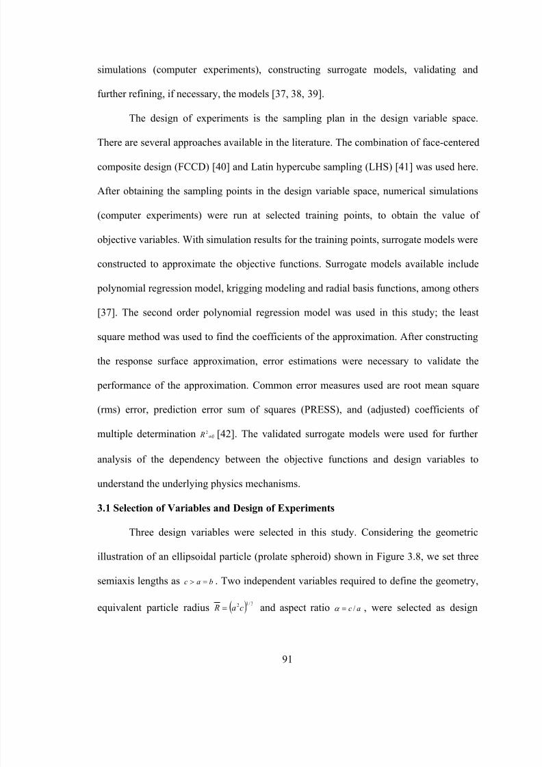
8/21/2019 zhangxc_1
http://slidepdf.com/reader/full/zhangxc1 108/178
91
simulations (computer experiments), constructing surrogate models, validating and
further refining, if necessary, the models [37, 38, 39].
The design of experiments is the sampling plan in the design variable space.
There are several approaches available in the literature. The combination of face-centered
composite design (FCCD) [40] and Latin hypercube sampling (LHS) [41] was used here.
After obtaining the sampling points in the design variable space, numerical simulations
(computer experiments) were run at selected training points, to obtain the value of
objective variables. With simulation results for the training points, surrogate models were
constructed to approximate the objective functions. Surrogate models available include
polynomial regression model, krigging modeling and radial basis functions, among others
[37]. The second order polynomial regression model was used in this study; the least
square method was used to find the coefficients of the approximation. After constructing
the response surface approximation, error estimations were necessary to validate the
performance of the approximation. Common error measures used are root mean square
(rms) error, prediction error sum of squares (PRESS), and (adjusted) coefficients of
multiple determination adj R 2 [42]. The validated surrogate models were used for further
analysis of the dependency between the objective functions and design variables to
understand the underlying physics mechanisms.
3.1 Selection of Variables and Design of Experiments
Three design variables were selected in this study. Considering the geometric
illustration of an ellipsoidal particle (prolate spheroid) shown in Figure 3.8, we set three
semiaxis lengths as bac => . Two independent variables required to define the geometry,
equivalent particle radius ( ) 3/12ca R = and aspect ratio ac /=α , were selected as design

8/21/2019 zhangxc_1
http://slidepdf.com/reader/full/zhangxc1 109/178
Figure 3.8: Geometric illustration of an ellipsoidal particle.
92

8/21/2019 zhangxc_1
http://slidepdf.com/reader/full/zhangxc1 110/178
Table 3.4: Design variables and design space.
93

8/21/2019 zhangxc_1
http://slidepdf.com/reader/full/zhangxc1 111/178
94
variables. The third design variable was potential sweep rate v . The range of the three
design variables is shown in Table 3.4. A spherical particle of radius mr μ 50 = was used in
the experimental work of Uchida et al. [18], thus the range of equivalent particle radii
was selected as a 20% perturbation around 5μm. The aspect ratio range was selected
based on the experimental observation of particle morphology by scanning electron
microscope (SEM). The selected potential sweep rate gave a charge/discharge rate of
2.7C to 3.6C, which falls into the range of high-power applications.
The two objective functions chosen in this study were the peak value of the
cyclically varying maximum von Mises stress maxσ (in megapascal and the time-averaged
resistive heat generation rate avg,r Q (in picowatts). In fatigue analysis, mean value of the
cyclically varying stress affects the number of cycles allowed before failure as well as the
peak value [43]. In this study, numerical simulation results showed that mean stress and
the peak value of the stress are highly correlated (the correlation coefficient is 0.992).
Therefore, only the peak value of stress is considered as an objective function. Time-
averaged resistive heat generation rate is the total resistive heat generation normalized by
the overall charge half cycle time.
For the design of experiments, 20 points in total were selected in the design space
defined in Table 3.4. Among these points, 15 of them are from FCCD and the remaining
5 points are from LHS. Numerical simulations were conducted on these 20 training points
using the models described in the previous sections to obtain intercalation-induced stress
and resistive heat.
3.2 Model Construction and Validation

8/21/2019 zhangxc_1
http://slidepdf.com/reader/full/zhangxc1 112/178
95
To construct the surrogate model using the obtained simulation results on the 20
training points, a second order polynomial response surface was selected. The
coefficients in the approximation were determined by minimizing the error of
approximation at the training points in the least square sense. The approximations
obtained for the two objective functions were
222
max 05.1079.000.255.2275.0065.013.410.881.40.18- vvv R R Rv R −−−+−−+++= α α α α σ (13)
222avg, 9.1809.3018.01.18816.017.20.8629.59.254.72 vvv R R Rv RQr +−−+−+−+−= α α α α
(14)
The statistics of the response surface approximation are listed in Table 3.5. RMS
error is the difference between the prediction and simulation values on the training points.
Adjusted coefficients of multiple determination adj R 2 are a measure of how well the
approximation explains the variation of the objective functions caused by design
variables. For a good fit, this coefficient should be close to one. PRESS is a cross-
validation error. It is the summation of squares of all PRESS residues, each of which is
calculated as the difference between the simulation by computer experiments and the
prediction by the surrogate models constructed from the remaining sampling points
excluding the point of interest itself [42]. As shown in Table 3.5, the normalized RMS
error and PRESS are small, and the adjusted coefficients of multiple determination adj R 2
is very close to one. Therefore, the surrogate models constructed approximate the
objective functions quite well.
To further validate the accuracy of constructed surrogate models, they were tested
by comparing the predicted and simulated values from computer experiments on four

8/21/2019 zhangxc_1
http://slidepdf.com/reader/full/zhangxc1 113/178
statistic name stress resistive heat
# of training points 20 20
minimum of data 11.7 1.96
mean of data 19.9 8.86
maximum of data 27.5 23.6
RMS error (normalized *) 0.0368 0.0168
R 2 adj 0.984 0.996
PRESS (normalized *) 0.0498 0.0356
* Note: RMS error and PRESS are both normalized by the range of the
objective functions, that is, the difference between the maximum and the
Table 3.5: Evaluation of the response surface approximations.
minimum of data.
96
8/21/2019 zhangxc_1
http://slidepdf.com/reader/full/zhangxc1 114/178
97
testing points different from the training points. The results of the comparison show that
the differences between the prediction and simulation results are within 6%.
To summarize, the surrogate models constructed (13) and (14) not only explain
the variation of objective functions resulting from design variables well, but also give a
good prediction of the objective functions. Therefore, the obtained response surface
approximations can be used with confidence to analyze dependencies among objective
functions and design variables.
3.3 Analysis Based on Obtained Surrogate Models
These dependencies are shown in Figure 3.9. We note that 1) intercalation-
induced stress maxσ increases with both increasing equivalent radius R and increasing
potential sweep rate v ; however, intercalation-induced stressmaxσ increases first and then
decreases as aspect ratio α increases; and 2) time-averaged resistive heat generation rate
avg,r Q increases with both increasing equivalent radius R and increasing potential sweep
rate v ; however, time-averaged resistive heat generation rate avg,r Q decreases as aspect
ratio α increases. This surrogate-based analysis suggests that ellipsoidal particles with
larger aspect ratios are superior to spherical particles for improving battery performance
when stress and heat generation are the only limiting factors considered.
As pointed out earlier, intercalation-induced stress depends on the concentration
distribution. When equivalent radius R increases, the range of concentration distributions
within the particle becomes wider, because of the longer diffusion path. Therefore, the
intercalation-induced stress increases as equivalent radius R increases. When potential
sweep rate v increases, the electrochemical reaction rate driven by the surface
8/21/2019 zhangxc_1
http://slidepdf.com/reader/full/zhangxc1 115/178
Figure 3.9: The dependency between objective functions and design
variables (a) maximum von Mises stress (in megapascal), (b) time-
averaged resistive heat rate (in picowatts).
98

8/21/2019 zhangxc_1
http://slidepdf.com/reader/full/zhangxc1 116/178
99
overpotential becomes faster, which results in large flux on the particle surface boundary.
Therefore, one expects a larger concentration gradient inside the particle and larger
intercalation-induced stress for larger potential sweep rate v . When aspect ratio α
increases, there are two competing effects: the shorter semi-axis lengths a and b decrease
and the longer semi-axis length c increases. The increase of the longer semi-axis leads to
stress increase, and the decrease of the shorter semi-axis leads to stress decrease.
Therefore, intercalation-induced stress increases first and then decreases as aspect ratio
increases.
As shown in Equation (10), resistive heat rate is the product of current and
overpotential (or polarization), and the time-averaged heat generation rate over the charge
half cycle is
( )∫ −Δ
= t U V I t
Qr d1 avg
charge
avg, . (15)
As the equivalent radius increases, the surface area subjected to reaction is larger, which
results in larger total current. Therefore, the averaged resistive heat generation rate
increases. When the potential sweep rate increases, the electrochemical reaction on the
surface is driven faster, which results in larger polarization, or overpotential. Therefore,
the averaged resistive heat generation rate increases even though the time duration for the
charge half cycle decreases. When the aspect ratio increases, the shorter semiaxis length
decreases; this results in the decrease of average polarization or overpotential due to the
shorter average diffusion path. Therefore, the averaged resistive heat generation rate
decreases.
Global sensitivity analysis, which is often used to study the importance of design
variables, was conducted to quantify the variation of the objective functions caused by

8/21/2019 zhangxc_1
http://slidepdf.com/reader/full/zhangxc1 117/178
100
three design variables. The importance of design variables is presented by main factor
and total effect indices [37]. Main factor is the fraction of the total variance of the
objective function contributed by a particular variable in isolation, while the total effect
includes contribution of all partial variances in which the variable of interest involved
(basically by considering those interaction terms in the response surface approximation as
shown in Equation (13) and (14)). The calculated total effect results are listed in Table
3.6. It can be seen that, for the design space range selected in Table 3.4, equivalent
particle radius contributes the most to the variation of the two objective functions,
intercalation-induced stress and resistive heat (85 and 87% of total variation respectively).
4. ASSUMPTION OF A UNIFORM ELECTRIC POTENTIAL
In the current model, electric potential inside the particle is assumed to be
uniform, though potential varies in a battery electrode particle due to electric current flow
within the particle. From a modeling standpoint, the most important value to accurately
estimate is the electric potential on the particle surface, because this value determines the
electrochemical reaction rate via the Butler-Volmer equation. The simulation presented in
this study follows an earlier microelectrode experimental work where an electric potential
is applied through a filament in contact with a cathode particle [18].
The potential distribution inside the particle could have been obtained numerically in
our model by solving Poisson’s equation. Experimentally [18], potential was measured at
a single point, but it is impractical to set up a similar boundary condition for the electric
potential numerically, because the applied potential is applied, ideally, at a single point.
To evaluate the significance of potential variation on the particle surface to the

8/21/2019 zhangxc_1
http://slidepdf.com/reader/full/zhangxc1 118/178
Table 3.6: Global sensitivity indices (total effect) for stress and
resistive heat.
101

8/21/2019 zhangxc_1
http://slidepdf.com/reader/full/zhangxc1 119/178
102
intercalation process, we use a prescribed potential variation in the numerical simulation
to investigate the significance of this variation.
The resistivity of LiMn2O4 is about 1.5×10⁴Ω-cm [44]. The peak value measured
current drawn from a 5μm (radius) particle under 4C discharge is on the order of 2nA
[18]. The electric potential variation inside a 5μm (radius) particle under 4C discharge is
on the order of 10mV, which is comparable to the surface overpotential obtained (Figure
3.4). To evaluate the importance of this potential variation, we apply a prescribed electric
potential to a 5μm (radius) particle. Figure 3.10 (a) shows the distribution of the potential
at time instant t=1534s. The prescribed spatial potential variation follows the equation
0.005(x2+y
2+(z-r 0)
2)/(2r 0)
2, where r 0 (in microns) is the radius of the particle.
Potentiodynamic control in this case has applied potential varying linearly with time.
Figure 3.10 (b) (c) (d) shows the simulation results of this case. The time history
of von Mises stress (Figure 3.10 (b)) follows the same trend, when the potential is
assumed to be uniform. The variation of electric potential results in a non-uniform
distribution of surface overpotential and surface reaction flux, which, in turn, results in a
shift in the concentration distribution as shown in Figure 3.10 (c). However, the
distribution pattern of von Mises stress is not altered; it remains axisymmetric as shown
in Figure 3.10 (d). The time instant of t=1534s is selected to present the results because
this is the instant when von Mises stress reaches the temporal maximum value.
To sum up, although the variation of electric potential shifts the concentration
distribution, it does not change von Mises stress distribution pattern. For simplicity and
due to lack of more detailed empirical guideline, we assume that the electric potential is
uniform inside the particle. Our finding does offer scientific insight into the interplay

8/21/2019 zhangxc_1
http://slidepdf.com/reader/full/zhangxc1 120/178
Figure 3.10: Simulation with a predescribed potential variation: (a)
otential variation on article surface at t=1534s, b time histor of
von Mises stress on particle surface, (c) concentration distribution
inside the particle at t=1534s, and (d) von Mises stress distribution
inside the particle at t=1534s.
103

8/21/2019 zhangxc_1
http://slidepdf.com/reader/full/zhangxc1 121/178
104
between stress and heat generation, particle geometry (aspect ratio and equivalent size),
and potential sweep rate.
5.
CONCLUSIONS
Intercalation-induced stress and heat generation inside Li-ion battery cathode
(LiMn2O4) particles under potentiodynamic control were simulated. It was found that Li-
ion concentration, surface flux, and intercalation-induced stress are highly correlated
through the diffusion process, electrochemical kinetics and the intercalation-induced
lattice expansion. The two peaks observed in the flux and stress generation plots were
attributable to intrinsic material properties (two plateaus in the OCP) and the applied
potential. Three major heat generation sources, resistive heating, heat of mixing and
entropic heat, were analyzed. The heat of mixing was found to be negligible (two orders
of magnitude smaller than the other two sources) and resistive heat was identified as the
heating source of greatest importance.
The surrogate-based analysis approach was used to study the relationship among
the two objective functions (intercalation-induced stress and resistive heat) and the
selected design variables (particle morphology and the operating condition). It was shown
that both intercalation-induced stress and time-averaged resistive heat generation rate
increase with increasing equivalent particle radius and potential sweep rate; intercalation-
induced stress increases first, then decreases, as the aspect ratio of an ellipsoidal particle
increases, while averaged resistive heat generation rate decreases as aspect ratio
increases. A sensitivity analysis was conducted to rank the importance of each design
variable on the stress and heat generation. It was shown that particle equivalent radius
contributes the most to both stress and heat generation for the design space range

8/21/2019 zhangxc_1
http://slidepdf.com/reader/full/zhangxc1 122/178
105
considered in this study (85 and 87% of the total variation, respectively). The observed
variation trend from this systematic numerical study may also be explained from
fundamental principles: intercalation-induced stress depends on the Li-ion concentration
distribution and the resistive heat depends on a combination of total charge current and
polarization (overpotential). The surrogate-based analysis conducted suggests that
ellipsoidal particles with larger aspect ratios are preferred over spherical particles in
improving battery performance, when stress and heat generation are the only factors
considered.
The proposed models in this study are only valid for purely active material
(LiMn2O4) without inclusions. The obtained results are fundamental, but for
homogeneous particles. The general methodology of surrogate-based analysis presented
in this study is extendable to consider more variables and geometries, such as more
complicated geometric representation (aggregates) and applied potential profiles
controlled by more parameters, or larger scales. In the next chapter, we will extend the
models, developed here at the particle scale, to the whole cell scale with a volume
averaging technique [45, 46, 47] in which a multiscale modeling methodology [48] will
be applied to pass the information obtained on the microscopic scale to the macroscopic
scale.

8/21/2019 zhangxc_1
http://slidepdf.com/reader/full/zhangxc1 123/178
106
BIBLIOGRAPHY
1. K. E. Thomas, and J. Newman, Thermal Modeling of Porous Insertion Electrodes,
Journal of the Electrochemical Society, 150, A176-A192 (2003).
2. H. Maleki, G. Deng, A. Anani, and J. Howard, Thermal Stability Studies of Li-
Ion Cells and Components, Journal of the Electrochemical Society, 146 (9) 3224-3229 (1999).
3. A. Du Pasquier, F. Disma, T. Bowmer, A.S. Gozdz, G. Amatucci, and J.-M.
Tarascon, Differential Scanning Calorimetry Study of the Reactivity of Carbon
Anodes in Plastic Li-Ion Batteries, Journal of Electrochemical Society 145, 472-477 (1998).
4. R. Spotnitz, and J. Franklin, Abuse Behavior of High-Power, Lithium-Ion Cells,
Journal of Power Sources, 113, 81-100 (2003).
5. M.-R. Lim, W.-I. Cho, and K.-B. Kim, Preparation and characterization of gold-codeposited LiMn2O4 electrodes, Journal of Power Sources, 92, 168-176 (2001).
6. D. Wang, X. Wu, Z. Wang, and L. Chen, Cracking Causing Cyclic Instability of
LiFePO4 Cathode Material, Journal of Power Sources, 140, 125-128 (2005).
7. H. Wang, Y.-I. Jang, B. Huang, D. R. Sadoway, and Y.-M. Chiang, TEM Study
of Electrochemical Cycling-Induced Damage and Disorder in LiCoO2 Cathodesfor Rechargeable Lithium Batteries, Journal of the Electrochemical Society, 146,
473-480 (1999).
8. Y.-M. Choi and S.-I. Pyun, Effects of Intercalation-Induced Stress on Lithium
Transport through Porous LiCoO2 Electrode, Solid State Ionics, 99, 173-183
(1997).
9. K. E. Aifantis and J. P. Dempsey, Stable crack growth in nanostructured Li-
batteries, Journal of Power Sources, 143, 203–211 (2005).
10. D. Bernardi, E. Pawlikowski, and J. Newman, A General Energy Balance for
Battery Systems, Journal of the Electrochemical Society, 132, 5-12 (1985).
11. Y. Chen and J.W. Evans, Three-Dimensional Thermal Modeling of Lithium-
Polymer Batteries under Galvanostatic Discharge and Dynamic Power Profile,
Journal of the Electrochemical Society, 141, 2947-2955 (1994).
12. S. C. Chen, C. C. Wan, and Y. Y. Wang, Thermal Analysis of Lithium-Ion
Batteries, Journal of Power Sources, 140, 111-124 (2005).
13. J. Christensen and J. Newman, Stress Generation and Fracture in Lithium
Insertion Materials, Journal of Solid State Electrochemistry, 10, 293–319 (2006).
14. R. E. Garcia, Y.-M. Chiang, W. C. Carter, P. Limthongkul, and C. M. Bishop,Microstructural Modeling and Design of Rechargeable Lithium-Ion Batteries,
Journal of the Electrochemical Society, 152, A255-A263 (2005).

8/21/2019 zhangxc_1
http://slidepdf.com/reader/full/zhangxc1 124/178
107
15. Y.-B. Yi, C.-W. Wang, and A. M. Sastry, Two-Dimensional vs. Three-Dimensional Clustering and Percolation in Fields of Overlapping Ellipsoids
Journal of the Electrochemical Society, 151, A1292-A1300 (2004).
16. X. Zhang, W. Shyy, and A. M. Sastry, Numerical Simulation of Intercalation-
Induced Stress in Li-Ion Battery Electrode Particles, Journal of theElectrochemical Society, 154, A910-A916 (2007).
17. A. Guerfi, P. Charest, K. Kinoshita, M. Perrier, and K. Zaghib, Nano
Electronically Conductive Titanium-Spinel as Lithium Ion Storage Negative
Electrode, Journal of Power Sources, 126, 163–168 (2004).
18. I. Uchida, H. Fujiyoshi, and S. Waki, Microvoltammetric Studies on SingleParticles of Battery Active Materials, Journal of Power Sources, 68, 139-144
(1997).
19. D. Zhang, B. N. Popov, and R. E. White, Modeling Lithium Intercalation of a
Single Spinel Particle under Potentiodynamic Control, Journal of TheElectrochemical Society, 147, 831-838 (2000).
20. K. E. Thomas, C. Bogatu, and J. Newman, Measurement of the Entropy of
Reaction as a Function of State of Charge in Doped and Undoped Lithium
Manganese Oxide, Journal of The Electrochemical Society, 148, A570-A575(2001).
21. I. Taniguchi, C.K. Lim, D. Song, and M. Wakihara, Particle Morphology and
Electrochemical Performances of Spinel LiMn2O4 Powders Synthesized Using
Ultrasonic Spray Pyrolysis Method, Solid State Ionics, 146, 239-247 (2002).
22. X. He, J. Li, Y. Cai, C. Jiang and C. Wan, Preparation of Spherical LiMn2O4
Cathode Material for Li-ion Batteries, Materials Chemistry and Physics, 95, 105-108 (2006).
23. W. Liu, G.C. Farrington, F. Chaput, and B. Dunn, Synthesis and Electrochemical
Studies of Spinel Phase LiMn2O4 Cathode Materials Prepared by the Pechini
Process, Journal of the Electrochemical Society, 143, 879-884 (1996).
24. S. H. Ju, D. Y. Kim, E. B. Jo, and Y. C. Kang, LiMn2O4 Particles Prepared bySpray Pyrolysis from Spray Solution with Citric Acid and Ethylene Glycol”,
Journal of Materials Science, 42, 5369-5374 (2007).
25. M. G. Lazarraga, S. Mandal, J. Ibanez, J. M.Amarilla, and J. M. Rojo, LiMn2O4-
based Composites Processed by a Chemical-route Microstructural, Electrical,
Electrochemical, and Mechanical Characterization, Journal of Power Sources,115, 315–322 (2003).
26. L. Fransson, T. Eriksson, K. Edström, T. Gustafsson and J. O. Thomas, Influence
of Carbon Black and Binder on Li-ion Batteries, Journal of Power Sources, 101,1-9 (2001).
8/21/2019 zhangxc_1
http://slidepdf.com/reader/full/zhangxc1 125/178
108
27. A. Momchilov, A. Trifonova, B. Banov, B. Pourecheva, and A. Kozawa, Nonaqueous UFC Suspensions, Used as Conductive Additive in Cathodes for
Lithium Batteries, Journal of Power Sources, 81–82 566–570 (1999).
28. K. Zaghib, J. Shim, A. Guerfi, P Charest, and K. A. Striebel, Effect of Carbon
Source as Additives in LiFePO4 as Positive Electrode for Lithium-Ion Batteries,Electrochemical and Solid-State Letters, 8, A207-A210 (2005).
29. Y.-H. Chen, C.-W. Wang, G. Liu, X.-Y. Song, V. S. Battaglia, and A. M. Sastry,
Selection of Conductive Additives in Li-Ion Battery Cathodes A Numerical
Study, Journal of The Electrochemical Society, 154, A978-A986 (2007).
30. T.H. Cho, S.M. Park, M. Yoshio, T. Hirai, Y. Hideshima, Effect of SynthesisCondition on the Structure and Electrochemical Properties of
Li[Ni1/3Mn1/3Co1/3]O2 Prepared by Carbonate Co-Precipitation Method,
Journal of Power Sources, 142, 306-312 (2005).
31. M. Higuchi, K. Katayama, Y. Azuma, M. Yukawa, M. Suhara, Synthesis ofLiFePO4 Cathode Material by Microwave Processing, Journal of Power Sources,
119-121, 258-261 (2003).
32. T. F. Fuller, M. Doyle, and J. Newman, Simulation and Optimization of the Dual
Lithium Ion Insertion Cell, Journal of the Electrochemical Society, 141, 1-10(1994).
33. J. Newman and K.E. Thomas-Alyea, Electrochemical Systems (third edition), pp.
209-212, John Wiley & Sons, New Jersey, 2004.
34. M. Doyle, J. Newman, A. S. Gozdz, C. N. Schmutz, and J.-M. Tarascon,
Comparison of Modeling Predictions with Experimental Data from Plastic
Lithium Ion Cells, Journal of the Electrochemical Society, 143, 1890-1903(1996).
35. M. M. Thackeray, Manganese Oxides for Lithium Batteries, Progress in Solid
State Chemistry, 25, l-71 (1997).
36. C. de Boor, Spline Toolbox 3 User's Guide, The MathWorks Inc., pp. 3.8, Natick,
MA, 2006.
37. N. V. Queipo, R. T. Haftka, W. Shyy, T. Goel, R. Vaidyanathan, and P. K.Tucker, Surrogate-based Analysis and Optimization, Progress in Aerospace
Sciences, 41, 1-28 (2005).
38. J. I. Madsen, W. Shyy and R. T. Haftka, Response Surface Techniques for
Diffuser Shape Optimization, AIAA Journal, 38, 1512-1518 (2000).
39. T. Goel, R. Vaidyanathan, R. T. Haftka, W. Shyy, N. V. Queipo, and K. Tucker,Response Surface Approximation of Pareto Optimal Front in Multi-Objective
Optimization, Computer Methods in Applied Mechanics and Engineering, 196,
879–893 (2007).
8/21/2019 zhangxc_1
http://slidepdf.com/reader/full/zhangxc1 126/178
109
40. G. E. P. Box and K. B. Wilson, On the Experimental Attainment of OptimumConditions, Journal of the Royal Statistical Society, Series B (Methodological),
13, pp. 1-45 (1951).
41. M. D. McKay and R. J. Beckman and W. J. Conover, A Comparison of Three
Methods for Selecting Values of Input Variables in the Analysis of Output from aComputer Code, Technometrics, 21, 239-245 (1979).
42. R. H. Myers, and D. C. Montgomery, Response Surface Methodology: Process
and Product Optimization Using Designed Experiments, pp. 17-48, John Wiley &
Sons Inc: New York, 1995.
43. N. E. Dowling, Mechanical Behavior of Materials: Engineering Methods forDeformation, Fracture, and Fatigue (second edition), pp. 357-400, Prentice Hall,
Upper Saddle River, NJ 1999.
44. Y. Shimakawa, T. Numata, and J. Tabuchi, Verwey-Type Transition and
Magnetic Properties of the LiMn2O4 Spinels, Journal of Solid State Chemistry,131, 138-143 (1997).
45. W. Shyy, S. S. Thakur, H. Ouyang, J. Liu, and E. Blosch, Computational
Techniques for Complex Transport Phenomena, pp. 231-258, Cambridge
University Press, New York, 1997.
46. A. R. Martin, C. Saltiel, W. Shyy, Heat Transfer Enhancement with PorousInserts in Recirculating Flows, Journal of Heat Transfer, 120, 458-467 (1998).
47. E. Sozer and W. Shyy, Modeling of Fluid Dynamics and Heat Transfer through
Porous Media for Liquid Rocket Propulsion, AIAA-2007-5549, 43rd
AIAA/ASME/SAE/ASEE Joint Propulsion Conference and Exhibit, Cincinnati,
OH, 2007.48. W. E, B. Engquist, X. Li, W. Ren, and E. Vanden-Eijnden, Heterogeneous
Multiscale Methods: a Review, Communications in Computational Physics, 2,
367-450 (2007).

8/21/2019 zhangxc_1
http://slidepdf.com/reader/full/zhangxc1 127/178
110
CHAPTER IV
SURROGATE-BASED SCALE BRDGING AND MICROSCOPIC SCALE
MODELING OF CATHODE ELECTRODE MATERIALS
1. INTRODUCTION
1.1. Challenges for Li-Ion Battery Modeling
Modeling of Li-ion batteries is of significant importance for both understanding
physicochemical characteristics of the electrochemical system and guiding design
optimization of batteries. However, modeling of Li-ion batteries is a challenging problem
due to the presence of two special characteristics of the electrochemical system,
multiphysics processes and disparate length and time scales.
A complicated electrochemical system like a Li-ion cell involves transport of ions
and electrons [1], electrochemical reactions on solid active material and liquid electrolyte
interface [1], heat generation and transfer [2], and intercalation-induced stress generation
[3]. The corresponding governing equations for these physicochemical processes are
coupled and the electrochemical kinetics is nonlinear. It is a nontrivial problem to solve
this coupled nonlinear equation system.
Modeling of Li-ion batteries also needs to deal with disparate length scales and
time scales. A battery typically consists of several cells. A schematic diagram and
dimensional scales for a cell and its components are shown in Figure 4.1. As can be seen
in Figure 4.1, along the thickness direction, scales range from 0.52 mm for the thickness

8/21/2019 zhangxc_1
http://slidepdf.com/reader/full/zhangxc1 128/178
(c)
Figure 4.1: Scales in Li-ion batteries: (a) dimension for a single cell, (b)
components and their dimensions inside a single cell along the thickness
direction, and (c) a SEM image for LiMn2O4 positive electrode.
111

8/21/2019 zhangxc_1
http://slidepdf.com/reader/full/zhangxc1 129/178
112
of a single cell to about 4 μm for the size of a single electrode particle. In this study, we
refer to the battery scale as macroscopic scale and electrode particle scale as microscopic
scale. It was shown in the numerical simulations of single particles [3], that solution for
concentration has a relative 2-norm error of 1.78×10⁻⁴
and solution for intercalation-
induced stress has a relative 2-norm error of 5.03×10⁻³
when 131 elements are used. For
the single cell shown in Figure 4.1, there are 6×10⁸ electrode particles. Consequently, it
requires 7.9×10¹⁰
elements to resolve all the microscopic scales to the electrode particle
level assuming each particle contains 131 finite elements. Therefore, it cost tremendous
computational power to resolve all the processes existing within each single electrode
particle. It is also practically unfeasible to do so given the computation capability of
existing computers. Time scales for physicochemical processes inside Li-ion batteries are
given in Table 4.1. As shown in Table 4.1, time scale spans from seconds to hours during
the cycling of batteries. From the modeling and numerical simulation point of view, very
small time steps are required to resolve the process with the smallest time scale, and a
large number of time steps are required to finish an entire discharge/charge cycle. In
other words, the cost for the simulation of this transient process is very expensive.
Special care has to be taken to devise a framework to tackle the disparate length and time
scales in the modeling of Li-ion batteries.
1.2.Review of the Existing Li-Ion Battery Modeling Work in the Literature
Li-ion battery models in the existing literature with different fidelity are reviewed.
There are equivalent-circuit-based models, physics-based pseudo 2D models, single
particle 3D models, and a mesoscale 3D model.

8/21/2019 zhangxc_1
http://slidepdf.com/reader/full/zhangxc1 130/178
a e . :
inside a Li-ion battery.
113
8/21/2019 zhangxc_1
http://slidepdf.com/reader/full/zhangxc1 131/178
114
Equivalent-circuit-based models, which originated from conventional electrochemical
impedance spectroscopy (EIS) battery characterization techniques, use an equivalent
electric circuit composed of resistors and capacitors to simulate cell performance and
behavior [4, 5, 6]. This category of models does not require detailed understanding of the
physicochemical mechanisms but requires certain parameters empirically fitted from
experimental measurement data. Equivalent-circuit-based models are capable of rapidly
predicting cell performance and behavior with simplified physics and adequate fidelity
[5]. However, these models are also criticized because no detailed modeling of
physicochemical processes is involved and they do not facilitate understanding of
physical mechanisms.
Pseudo 2D models were first developed from porous electrode theory [7] by
solving continuum scale governing equations for all the physicochemical processes over
homogeneous media along the thickness direction of a cell [8]. The required effective
material properties are commonly modeled by the classical Bruggeman equation. The
volumetric reaction rate is calculated using a simplified separated spherical electrode
particle by introducing a pseudo dimension. This category of models has been very
successful not only for predicting cell performance and behavior but also for
understanding the physical mechanisms of Li-ion batteries [9, 10, 11]. However, these
models use oversimplified assumptions and models for effective material properties and
volumetric reaction rates without detailed modeling of the microstructure architecture of
electrode materials.
As an attempt to model the detailed 3D microstructure of electrode materials, a
single electrode particle model was developed to model the intercalation-induced stress
8/21/2019 zhangxc_1
http://slidepdf.com/reader/full/zhangxc1 132/178
115
and heat generation inside ellipsoidal cathode particles during the discharge and recharge
cycles [3, 12]. This single particle numerical study showed that ellipsoidal particles with
larger aspect ratios are preferred to reduce stress and heat generation. A mesoscale
modeling approach was also proposed to implement the 3D detailed modeling of
electrode materials consisting of regularly and randomly arranged cathode particles [13].
The results agreed well with experimental testing data. However, the amount of electrode
particles included in the model was limited due to the excessive computation power
requirement.
In summary, it appears that the multiphysics problem has been successfully
addressed in the literature. However, the problem of disparate length and time scales has
not been sufficiently studied to allow for detailed microstructural modeling of electrode
architecture.
1.3. The Objectives of This Study
In this study, we will focus only on the treatment of disparate length scales to
study the effect of microstructure. We will tackle the problem of disparate time scales by
using sufficiently small time steps, assuming that we could afford conducting many time
steps advancing temporally. To address the disparate length scales in modeling of Li-ion
batteries, we set up the following objectives in this study.
(1) Develop a multiscale framework for Li-ion battery modeling to efficiently
account for the effects of electrode microstructural architecture;
(2) Conduct microscopic modeling of electrode particle clusters and solve the
closure terms in macroscopic scale governing equations as a first step toward
implementing the multiscale framework.

8/21/2019 zhangxc_1
http://slidepdf.com/reader/full/zhangxc1 133/178
116
2. METHODS
2.1. Li-Ion Cell Cycling Mechanisms and Governing Equations on Microscopic
Scale
2.1.1. Li-Ion Battery Fundamentals
A Li-ion cell typically consists of the following components: positive and
negative electrodes, a separator that isolates the two electrodes, and current collectors for
both electrodes. Electrodes are typically made of particles glued together by binders.
Pores inside electrodes and separator are commonly filled with liquid electrolyte that acts
as a pathway for Li ions. Figure 1.1 shows a diagram for the components of a Li-ion cell
and basic operation mechanisms for discharge/recharge cycling. During discharge of a
cell, Li ions are extracted (deintercalated) from the negative electrode, transported
through the electrolyte and finally inserted (intercalated) into the positive electrode.
Meanwhile, electrons move from the negative electrode to the positive electrode through
the external circuit and output work to the load. During recharge of a cell, Li ions and
electrons are transferred in the reverse direction as opposed to the discharge process. This
consumes work from the power supply to move the electrons. Intercalation and
deintercalation comprise electrochemical reactions on the interface of solid active
material and liquid electrolyte, diffusion of ions in the solid active material, and transport
of electrons in the solid active material.
2.1.2.Transport Processes
The effect of existing electrons in solid active material on the species flux of
lithium is assumed to be negligible because electrons are much more mobile than

8/21/2019 zhangxc_1
http://slidepdf.com/reader/full/zhangxc1 134/178
117
intercalated atoms [14]. The chemical potential gradient is the driving force for the
movement of lithium ions. Li ion transport is given as [14]
J = cv = − Mc∇μ , (1)
where v is the velocity of ion movements, is the mobility of lithium ions, c is the
concentration of Li ions, and μ is the chemical potential. Chemical potential depends on
concentration, temperature, and stress field. In this study, only concentration-driven
diffusion is considered. The governing equation for Li ion transport in solid active
materials is then given by
∂c1
∂t + ∇⋅ − D
1∇c
1( )= 0 , (2)
where D is the diffusion coefficient of Li ions in the solid active materials and subscript
1 indicates variables for solid phase.
For the transport of lithium ion in the electrolyte, the concentrated solution theory
is applied. The convection effect is neglected, and the species equation reads [1]
∂c2
∂t = ∇ ⋅ D
2∇c
2( )−
i2 ⋅ ∇t +
0
F , (3)
where subscript 2 indicates variables for liquid phase, i2
is the electric current in the
liquid phase and 0
+t is the transference number of lithium ions in solution and is assumed
to be constant in this study. In other words, the last term on the right hand side of
Equation (3) can be neglected.
The electron transport in the solid active material is governed by Poisson’s
equation
∇⋅ i1 = ∇⋅ σ
1∇V
1( )= 0 , (4)
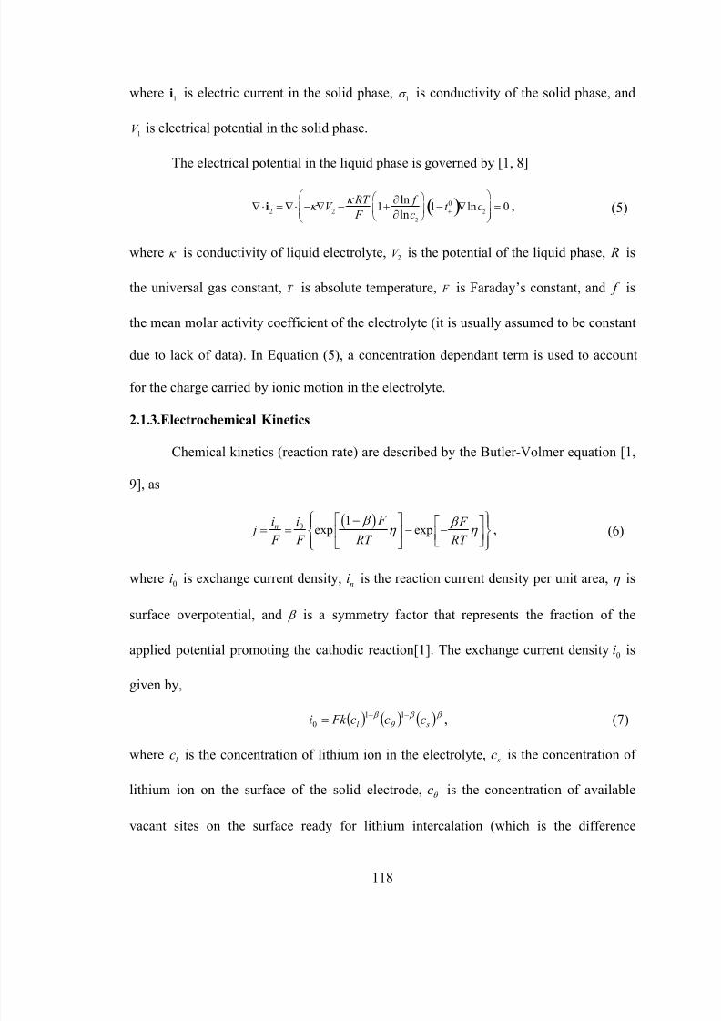
8/21/2019 zhangxc_1
http://slidepdf.com/reader/full/zhangxc1 135/178
118
where i1 is electric current in the solid phase, σ
1 is conductivity of the solid phase, and
V 1 is electrical potential in the solid phase.
The electrical potential in the liquid phase is governed by [1, 8]
∇⋅ i2 = ∇⋅ −κ ∇V
2 −
κ RT
F 1+
∂ ln f
∂ lnc2
⎛
⎝ ⎜
⎞
⎠⎟ 1− t +
0( )∇ lnc2
⎛
⎝ ⎜⎜
⎞
⎠⎟⎟ = 0 , (5)
where κ is conductivity of liquid electrolyte, V 2 is the potential of the liquid phase, R is
the universal gas constant, T is absolute temperature, F is Faraday’s constant, and f is
the mean molar activity coefficient of the electrolyte (it is usually assumed to be constant
due to lack of data). In Equation (5), a concentration dependant term is used to account
for the charge carried by ionic motion in the electrolyte.
2.1.3.Electrochemical Kinetics
Chemical kinetics (reaction rate) are described by the Butler-Volmer equation [1,
9], as
( )01
exp expn F i i F
j F F RT RT
β β η η
⎧ ⎫⎡ ⎤−⎪ ⎪⎡ ⎤= = − −⎨ ⎬⎢ ⎥ ⎢ ⎥⎣ ⎦⎪ ⎪⎣ ⎦⎩ ⎭ , (6)
where i0 is exchange current density, ni is the reaction current density per unit area, η is
surface overpotential, and β is a symmetry factor that represents the fraction of the
applied potential promoting the cathodic reaction[1]. The exchange current density i0 is
given by,
( ) ( ) ( ) β β θ
β sl ccc Fk i −−= 11
0 , (7)
where cl is the concentration of lithium ion in the electrolyte, c s is the concentration of
lithium ion on the surface of the solid electrode, cθ is the concentration of available
vacant sites on the surface ready for lithium intercalation (which is the difference

8/21/2019 zhangxc_1
http://slidepdf.com/reader/full/zhangxc1 136/178
119
between stoichiometric maximum concentration and current concentration on the surface
of the electrode cmax − c s ), and k is a reaction rate constant [9]. Surface overpotential η
is given, without considering film resistance, by [9]
η = V 1 − V
2 − U , (8)
where V 1 and V
2 are electric potential for the solid and liquid phase respectively, andU is
the open-circuit potential, which depends on lithium ion concentration.
2.1.4.Intercalation-induced Stress Generation
When Li ions are intercalated into the lattice of active material in electrodes, the
lattice is expanded accordingly. This lattice expansion causes strain inside the material.
Non-uniform strain results in stress, the so-called intercalation-induced stress. To model
this intercalation-induced stress, an analogy to thermal stress is proposed [3]. The
constitutive equation between stress and strain is [3]
( )1
13
ij ij kk ij ij E
cε ν σ νσ δ δ = + − +
Ω⎡ ⎤⎣ ⎦
(9)
where ε ij are strain components, σ
ij are stress components, E is Young’s modulus, ν is
Poisson’s ratio, c = c − c0 is the concentration change of the diffusion species (lithium
ion) from the original (stress-free) value, and Ω is the partial molar volume of lithium.
Stress components are subjected to the force equilibrium equation
σ ij , i
= 0 ( j = 1, 2, 3) . (10)
A Young’s modulus E = 10GPa and a partial molar volume Ω = 3.497 × 10⁻⁶ m3 /mol [3]
are used here.
2.1.5.Heat Generation and Transfer

8/21/2019 zhangxc_1
http://slidepdf.com/reader/full/zhangxc1 137/178
120
There are four sources of heat generation inside lithium ion batteries during
operation [15]
Q g = I V − U
avg
( )+ IT
∂U avg
∂T + Δ H
k
avgr
k +
k ∑ H
ij − H
ij
avg
( )
∂cij
∂t i∑ j∑dv
∫ (11)
The first term, I V − U avg( ), is the irreversible resistive heating, where I is the current of
the cell, V is the cell potential, and avgU is the volume averaged open circuit potential.
Resistive heating is caused when the cell potential deviates from its equilibrium because
of resistance to the passage of current. The second term, T U IT ∂∂ avg , is the reversible
entropic heat, where T is temperature. The third term, ∑Δk
k
avg
k r H , is the heat change of
chemical side reactions, where avg
k H Δ is the enthalpy of reaction for chemical reaction k ,
and k r is the rate of reaction k . The fourth term, ( )∫∑∑ ∂∂− vt c H H dij
j i
avg
ijij, is the heat of
mixing due to the generation and relaxation of concentration gradients, whereij
c is the
concentration of species i in phase j, vd is the differential volume element, and ij H and
avg
ij H are the partial molar enthalpy of species i in phase j and the averaged partial molar
enthalpy respectively. The study conducted on single particles showed that heat of
mixing is negligible compared to resistive heat and entropic heat [12]. Therefore, there
are only two heat generation sources of significance, resistive heat and entropic heat,
without considering heat change due to side reactions.
Heat transfer inside Li-ion batteries can be modeled by the conventional heat
conduction equation [16, 17],
p x y z
T T T T C k k k Q
t x x y y z z ρ
∂ ∂ ∂ ∂ ∂ ∂ ∂= + + +
∂ ∂ ∂ ∂ ∂ ∂ ∂
⎛ ⎞⎛ ⎞ ⎛ ⎞⎜ ⎟ ⎜ ⎟⎜ ⎟⎝ ⎠ ⎝ ⎠⎝ ⎠
, (12)

8/21/2019 zhangxc_1
http://slidepdf.com/reader/full/zhangxc1 138/178
121
where ρ is density, C p
is heat capacity, and k x , k y , k z are heat conductivity along x, y and
z directions respectively. Heat conductivity is generally anisotropic for battery materials
due to different components inside batteries.
2.2. Multiscale Modeling Framework
2.2.1.Volume Averaging Technique
The main objective of multiscale modeling is to capture the physics to a certain
desired accuracy in an efficient way. Microscopic models are accurate but
computationally expensive, while macroscopic models are simplified and efficient. The
combinational use of models on these two scales will help to achieve accuracy and
efficiency at the same time. Microscopic and macroscopic models could be
fundamentally different in terms of the physics principles applied. For example, one
could apply molecular dynamics to the microscopic scale and continuum fluid dynamics
to the macroscopic scale. Sometimes, one basic physics principle is applicable for all
scales and scale disparity is caused by the geometric complexity, which is the case for the
processes in porous electrode materials. For the multiscale modeling of the processes in
porous media, there are two approaches that can be adopted to derive the macroscopic
governing equations from their counterparts on the microscopic scale, volume averaging
[18] and homogenization [19][20]. The volume averaging technique is used in this study.
In the volume averaging technique, the variable of interest is first averaged over a
representative elementary volume (REV). The governing equations on the microscopic
scale are then averaged over REV. In the differential equations, the volumetric averages
of the temporal and spatial derivatives are transformed into the temporal and spatial
derivatives of the averaged quantities by using the two theorems dealing with the

8/21/2019 zhangxc_1
http://slidepdf.com/reader/full/zhangxc1 139/178
122
averages of derivatives [18]. There are additional closure terms, which require further
modeling, appearing as the consequence of the averaging process. Volume averaging has
been widely used for modeling fluid flow and transport in porous media [18, 21]. Volume
averaging-like techniques have been applied for battery modeling to deal with the porous
feature of electrode materials [8, 9, 22, 23]. However, closure terms for effective material
properties and volumetric reaction rate have only been treated analytically using
oversimplified assumptions instead of detailed numerical modeling of microstructural
architecture.
There are two types of volume averages, defined as
Intrinsic volume average
c s
s=
1
dV sc sγ s
dV ∫ dV , (13)
where dV is the volume of REV, γ s = 1 in phase s and 0 elsewhere.
Volume average
c s = 1dV c sγ sdV ∫ dV , (14)
These two averages are related as
c s
s= g s c s (15)
where g s is the volume fraction of phase s.
When the volume averaging technique is applied to partial differential equations,
volume averages of temporal and spatial derivatives need to be transformed into
derivatives of volume averages of variables following these two theorems,
1
dV
∂c s
∂t
⎛
⎝ ⎜ ⎞
⎠⎟γ s
dV ∫ dV =
∂c s
∂t −
1
dV c sv ⋅n
As
∫ d A , (16)

8/21/2019 zhangxc_1
http://slidepdf.com/reader/full/zhangxc1 140/178
123
1
dV ∇⋅ D s∇c s( )γ sdV ∫ dV = ∇⋅ D s∇c s( )+ 1
dV D s∇c s( )⋅n
As
∫ d A ,
(17)
where v is the velocity of the microscopic interface and n is the outward unit norm of the
infinitesimal area element d A , if the terms in a transient diffusion equation is used for an
example. In Li-ion battery modeling, the movement of solid active material and liquid
electrolyte phase interface is negligible, which means the second term 1 dV c sv ⋅nd A As∫ on
the right side of Equation (16) vanishes. In Equation (17), two closure terms on the right
side of the equation need special treatment. ∇⋅ D s∇c s( ) is the gradient of the averaged
diffusion flux. Traditionally, the average of diffusion flux resulting from the
concentration gradient is modeled by introducing a so-called effective diffusivity,
D s∇c s = D seff ∇c s , (18)
and the effect diffusivity is conventionally modeled analytically using classical
Bruggeman’s relation
D seff = D s
bulk g sα , (19)
where D s bulk is the bulk diffusivity of homogeneous materials without inclusions, and α
is Bruggeman’s coefficient that is normally assumed to take the value of 1.5. However, it
has been shown that a Bruggeman exponent of 1.5 is often invalid for real electrode
materials [24]. In this study, we propose to calculate the volume average of the diffusion
flux or the effective diffusivity directly from 3D microscopic scale simulations instead of
modeling them analytically. The second term on right side of Equation (17) is the integral
of diffusion flux over the phase interface. In Li-ion battery modeling, this term accounts
for the flux due to electrochemical reaction on the interface of solid active material and
liquid electrolyte. Therefore, the term of J = 1 dV D s∇c s( )⋅nd A As∫ is actually the Li ion

8/21/2019 zhangxc_1
http://slidepdf.com/reader/full/zhangxc1 141/178
124
production or consumption per unit volume due to electrochemical reaction, and this term
is called the volumetric reaction rate. In the conventional pseudo 2D models, this
volumetric reaction rate term has been modeled using a simplified geometry of an
isolated spherical particle as [8]
s n J a j= , (20)
where a s = 3 g
s r
sis the specific interfacial area (per unit volume) of an isolated spherical
particle with radius r s
given the solid phase volume faction g s
, and n j is the reaction flux
per unit area calculated by Butler-Volmer equation (Equation (6)) using the volume
averaged Li-ion concentration in the liquid electrolyte, volume averaged electrical
potential in both liquid and solid phases, and Li ion concentration on an isolated spherical
particle surface by solving the diffusion equation on a pseudo dimension. In other words,
Equation (20) assumes that
( )s s
1 2 1 2
1 2 1 2 1 2 1 2
(c , c , V , V )
3d(c , c , V , V ) (c , c , V , V )
d
1 d d 1 d d
sn n
s
s s n A A
J
g A j j
V r
V D c A V j A= =
≈ ≈
∇ ⋅∫ ∫n
, (21)
where reaction flux 1 2 1 2(c , c , V , V )n j is calculated by Butler-Volmer equation using local
concentrations and electric potentials, and 1 2 1 2(c , c , V , V )n j is calculated by Butler-Volmer
equation using local Li ion concentration in the solid phase, volume averaged Li ion
concentration in the liquid phase, and volume averaged electric potentials in both phases.
A trivial case where Equation (21) holds would be the case where all the concentrations
and electrical potentials are uniformly distributed on the microscopic scale, and
electrodes are made of isolated spherical particles. The treatment for this volume
averaged reaction rate could be improved by direct calculation from microscopic scale

8/21/2019 zhangxc_1
http://slidepdf.com/reader/full/zhangxc1 142/178
125
modeling and simulations, which is the focus of this study. Details about coupling
between microscopic scale and macroscopic scales will be discussed in the section on
scale bridging.
For the sake of clarity and completeness, the derivation of governing equations
using the volume averaging technique will be described here even though similar
derivations have been given in [22, 23]. The derivation of macroscopic governing
equations using the volume averaging technique is presented as follows.
(1) Transport of Lithium Ions inside Liquid Electrolyte Phase
When the transference number0
+t is assumed to be constant, the transport
equation for lithium ion concentration is simplified as
∂c2
∂t = ∇⋅ D2∇c2( ). (22)
Take the volume average of both sides,
1
dV
∂c2
∂t
⎛
⎝ ⎜
⎞
⎠⎟ γ
2dV ∫ dV = 1
dV ∇⋅ D
2∇c
2( )γ 2
dV ∫ dV . (23)
With the theorems for the time derivative term and divergence term in volume averaging
technique, Equation (23) becomes
∂c2
∂t = ∇⋅ D2∇c2( )+ 1
dV D2∇c2( )⋅n
As
∫ d A +1
dV c2v ⋅n
As
∫ d A . (24)
Neglect the movement of the interface (i.e. 0=⋅ nv ), rewrite the average flux as
D2∇c2 = D2
eff ∇c2 , and use J c2to represent volumetric rate, one transforms Equation (24) into
∂c2
∂t = ∇⋅ D2
eff ∇c2( )+ J c2. (25)
(2) Electrical Potential inside Liquid Electrolyte Phase

8/21/2019 zhangxc_1
http://slidepdf.com/reader/full/zhangxc1 143/178
126
The transport equation for the electric current inside the liquid electrolyte
Equation (5) can be re-written as,
∇⋅ κ ∇V 2 +κ D∇ lnc2( )⎡⎣
⎤⎦ = 0 , (26)
where κ D
=κ RT
F 1+
∂ ln f
∂ lnc2
⎛
⎝ ⎜
⎞
⎠⎟ 1− t +
0( ) . Take the volume averaging over the left side of
Equation (26),
1
dV ∇⋅ κ ∇V 2 +κ D∇ lnc2( )⎡
⎣ ⎤
⎦γ 2dV ∫ dV = ∇⋅ κ ∇V 2 +κ D∇ lnc2( )( )+ 1
dV κ ∇V 2 +κ D∇ lnc2( )( )⋅n
As
∫ d A , (27)
J V 2= 1 dV ( ) κ ∇V 2 + κ D∇ lnc2( )( )⋅ n
As
∫ d A is the volume averaged reaction current at the interface,
and κ ∇V 2 +κ
D∇ lnc
2( )could be modeled as ( )2 2lneff eff
DV cκ κ ∇ + ∇ . Following [22],
2lnc could be
approximated using Taylor series expansion as
( )2 2
2 2 2 2 2 2 2
2
1 1 1ln ln d ln d ln
V V
c c V c c c V g cV V c
⎡ ⎤= ≈ + − =⎢ ⎥
⎣ ⎦∫ ∫ , (28)
thus Equation (27) becomes
( ) 22 2 2ln 0eff eff
D V V g c J κ κ ⎡ ⎤⎢ ⎥⎣ ⎦∇ ⋅ ∇ + ∇ + = . (29)
(3) Transport of Lithium Ions inside Solid Active Material Phase
Applying the volume averaging technique to Equation (2) for diffusion of Li ions
in solid phase with a similar procedure as that done for transport in liquid phase, Equation
(22), we have the volume averaged equation for Equation (2) as
∂c1
∂t = ∇⋅ D1eff ∇c1
( )+ J c1 , (30)
where1c J is the volume averaged reaction rate.
(4) Transport of Electrons inside Solid Active Material Phase

8/21/2019 zhangxc_1
http://slidepdf.com/reader/full/zhangxc1 144/178
127
Apply the volume averaging technique to the electrical potential equation in solid
phase Equation (4), and notice that
1
dV ∇⋅ σ ∇V 1( )γ 1
dV
∫ dV = ∇⋅ σ ∇V 1( )+1
dV σ ∇V 1( )⋅n
As
∫ d A , (31)
one obtains,
∇⋅ σ ∇V 1( )+1
dV σ ∇V 1( )⋅n
As
∫ d A = 0 , (32)
σ ∇V 1 could be modeled as σ eff ∇V
1 where σ eff is effective conductivity. Term
1/ dV ( ) σ ∇V 1( )⋅n As
∫ d A is a volume averaged boundary reaction current that can be represented
by J V 1
. Consequently, Equation (32) turns to
σ eff ∇V 1 + J V 1= 0 . (33)
In Equation (33), effective conductivity eff σ and volumetric reaction flux J V 1are two
closure terms requiring special treatment.
2.2.2.Scale Bridging
As shown in the previous subsection, there are some closure terms requiring
special treatment in the volume averaged governing equations. These terms are the
effective material properties,eff
D2 , eff κ , eff Dκ ,
eff D1 , and eff σ ; and volume averaged
reaction rates,2c J , J V 2
,1c J , and J V 1
. These closure terms highly depend on the detailed
microstructural architecture of electrode materials. In this study, we propose to calculate
the closure terms, based on their definitions, directly from 3D microscopic scale
simulations.
Following the scale bridging concept from [25, 26], a REV on the microscopic
scale is assigned to each integration point of the macro-mesh. Appropriate boundary

8/21/2019 zhangxc_1
http://slidepdf.com/reader/full/zhangxc1 145/178
128
conditions, derived from information available from the macroscopic scale, are imposed
on REV on the microscopic scale. A separate computation is then conducted for the REV,
and the obtained variable values are averaged over REV to provide macroscopic closure
terms with which the governing equations on macroscopic scale are solved. This provides
an approach to determine the macroscopic response of heterogeneous materials with
accurate accounting of micro-structural characteristics.
There are two categories of approaches to couple microscopic and macroscopic
scales, concurrent coupling and serial coupling [27]. In the concurrent coupling approach,
microscopic and macroscopic models are conducted concurrently with simultaneous
information exchange. In serial coupling, an effective macroscopic model is determined
from the microscopic model in a pre-processing step. It is expensive to conduct
microscopic and macroscopic scale simulations concurrently since microscopic scale
simulations are generally time consuming (in the case of battery modeling,
microstructural information of electrode materials needs to be resolved). Therefore, in
this study we preferred to adopt the serial coupling approach. To systematically arrange
the simulations on microscopic scale and couple the two scales efficiently, the database
approach [28] and look up table approach [29] have been used to map the microscopic
information and macroscopic closure terms. In this study we propose a surrogate-based
approach to bridge the scales serially. Surrogate-based approaches have been used for
design optimization and analysis [30]. Surrogate models are constructed using numerical
results obtained from simulations on carefully sampled points; they are capable of
predicting the objective functions efficiently over the whole design space once these
models are validated for sufficient accuracy. In applying a surrogate-based approach for

8/21/2019 zhangxc_1
http://slidepdf.com/reader/full/zhangxc1 146/178
129
scale bridging in battery modeling, the input variables for the surrogate models are the
microscopic structure information (such as volume fraction, aspect ratio of particles and
equivalent particle radius) and boundary conditions, for microscopic scale simulations,
from the nodes values on macroscopic scale mesh, and the output variables are those
closure terms calculated from microscopic scale simulations, as illustrated in Figure 4.2.
Details of surrogate-based scale bridging will be discussed in section 2.4.
2.3. 3D Microscopic Modeling of Electrode Particle Clusters
2.3.1.Microstructural Geometry Generation
To model the microstructural architecture, we use a collision-driven molecular
dynamics algorithm [31] to generate clusters of electrode particles. A certain number of
identical ellipsoidal particles with specified aspect ratio are packed inside a cubic box.
Since electrolyte does not contribute to conduction of electrons, to create a continuous
path for electron conduction the semi axes of these particles are multiplied by a
coefficient (1.1 is used in this study) to create an artificial overlapping between particles.
Those parts of the particles falling outside of the box are cut out. The remaining portion
of the particle cluster consists of the solid active material phase of the electrode
microstructure. The void space inside the cubic box not occupied by the particle cluster
consists of the liquid electrolyte phase.
2.3.2.Microstructural Geometry Characterization Parameters
In this study, microstructure of the representative volume element is primarily
characterized using volume fraction of solid phase, equivalent radius of solid particles,
and aspect ratio of prolate solid particles. Volume fraction determines how much active
material is available in the electrode and decides the maximum possible capacity of a

8/21/2019 zhangxc_1
http://slidepdf.com/reader/full/zhangxc1 147/178
s c a l e
n s
k .
t u r e
o n
m a c r o s c o p i
s i m u l a t i
o d e l i n g f r a m e w o r
m i c r o s t r u
c
i n f o r m a t i
b o u n d a r y
c o n d i t i o n s
c l o s u r e
t e r m s
i n g f o r m u l t i s c a l e
s u
r r o g a t e
m
o d e l s
- b a s e d
s c a l e b r i d
o p i c s c a l e
l a t i o n s
g u r e 4 . 2 : S u r r o g a t
m i c r o s
s i m
F i
130

8/21/2019 zhangxc_1
http://slidepdf.com/reader/full/zhangxc1 148/178
131
cell. On the other hand, volume fraction of solid phase also dictates the volume fraction
of its counterpart, the liquid electrolyte phase. In the case of too small a volume fraction
for liquid electrolyte, Li ions in the liquid electrolyte are depleted very quickly and cell
performance is limited by transport of ions in the liquid electrolyte phase. Equivalent
radius of ellipsoidal particles is defined as the radius of a sphere with the same volume.
The equivalent particle size decides the characteristic length and time for diffusion;
diffusion can be a limiting factor of battery performance, especially at very high cycling
rates. In this study, we only consider ellipsoidal particles in prolate shape. The aspect
ratio of a prolate particle is defined by the ratio between the long and short semi-axes.
The surface area of a prolate particle with fixed volume increases as the aspect ratio
increases. Therefore, the aspect ratio of particles actually determines the specific
interfacial area available for electrochemical reaction and is an important characteristic
for microstructure.
2.3.3.Governing Equations, Boundary Conditions, Material Properties and
Implementation
The governing equations solved for 3D microscopic simulations over REV are
Equation (2), (3), (4), (5), and (6). Steady state solutions are pursued. In other words, the
unsteady terms from temporal derivatives are not solved in Equation (2) and (3). As
described earlier, the boundary conditions take the node value from macroscopic scale
simulations. The interface of solid and liquid phases has diffusional and current flux
given by the Butler-Volmer equation. All other boundaries of the cubic box are set to be
symmetric without net flux of electrons or ions.

8/21/2019 zhangxc_1
http://slidepdf.com/reader/full/zhangxc1 149/178
l e s i m u l a t i o n s .
D
m i c r o s c o p i c s c
r i a l p r o
p e r t i e s f o r
T a b l e 4 . 2 : M a t
132

8/21/2019 zhangxc_1
http://slidepdf.com/reader/full/zhangxc1 150/178
133
LiMn2O4 is selected as the active material for the cathode, and LiPF6 in EC:DMC is
selected as the electrolyte. Material properties used for simulations are summarized in
Table 4.2.
The governing equations and boundary conditions are implemented in COMSOL
Multiphysics®
. Separate geometries are created for the solid and liquid phases
respectively. The coupling between the two phases are implemented using the ‘Extrusion
Coupling Variables’ capability in COMSOL Multiphysics®. The concentration and
electric potential of the liquid phase at the two phase interface boundary are mapped to
the boundary of the solid phase. This enables the calculation of reaction flux at the solid
phase boundary by the Butler-Volmer equation. The calculated reaction flux is then
mapped from the solid phase boundary to the liquid phase boundary, where the specified
flux boundary condition is assigned for the transport equations of electrons and ions. This
is a two-way coupling between the two phases; the coupling in both ways is carried out
simultaneously when the governing equations are solved.
2.4. Surrogate-Based Scale Bridging
Surrogate models are used to rapidly predict the closure terms in macroscopic
governing equations. The input variables (design variables) for surrogate models are the
microstructural information and boundary conditions for microscopic scale simulations;
the output variable (objective function) is the volumetric reaction rate. Surrogate models
are constructed based on 3D microscopic simulations as described in the previous section.
In this study, the microstructural information (volume fraction, aspect ratio of particles
and equivalent radius of particles) is considered as fixed to reduce the dimensionality of
the surrogate modeling problem. The concept demonstrated in this study could be easily

8/21/2019 zhangxc_1
http://slidepdf.com/reader/full/zhangxc1 151/178
134
extended to include microstructure information. The key steps of surrogate modeling
include design of experiments, running numerical simulations (computer experiments),
construction of surrogate models, validation and further refinement of the models if
necessary [30, 32, 33].
The design variables (boundary conditions for microscopic scale) are the
concentration and its gradient of Li ions and the electric potential and its gradient in both
solid and liquid phases. The ranges of the design variables are listed in Table 4.3, where
normalized Li ion concentration 1 1 total/=c c c in the solid active material phase is used and
is equivalent to the state of charge y. The ranges of variables are decided based on their
corresponding values in the possible pseudo 2D model solutions for cycling rates up to
3C. In Table 4.3, the variables of concentration and potential themselves are assigned to
the center of a REV; the gradients of variables that carry the information of variable
distribution are used, along with the variable values at the center of the REV, to calculate
the values on the top and bottom boundaries of the REV. In the ideal case, the values of
these variables come from solving the macroscopic governing. In this study, we assign
the values arbitrarily without considering the constraint of the macroscopic scale
governing equations, except for a constraint for solid phase concentration and electric
potential, 1 10.2 ( ) 0.2− ≤ − ≤V U c , in order to avoid numerical convergence issues
potentially caused by the exponential terms in the Butler-Volmer equation. In the
constrained design space, 189 points are selected by Latin hypercube sampling, and 128
points are selected at the corners of the design space to cover the boundary regions.
Numerical simulations on microscopic scale are run on these sampled points.
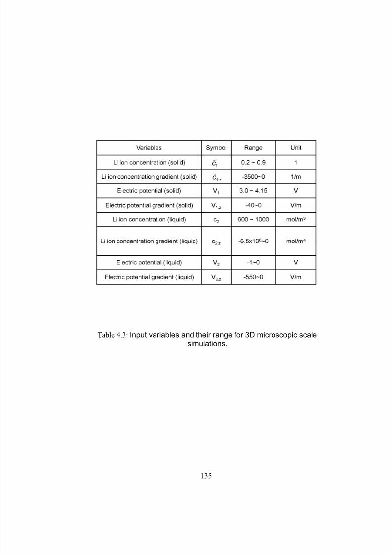
8/21/2019 zhangxc_1
http://slidepdf.com/reader/full/zhangxc1 152/178
Table 4.3: Input variables and their range for 3D microscopic scale
simulations.
135

8/21/2019 zhangxc_1
http://slidepdf.com/reader/full/zhangxc1 153/178
136
The obtained simulations results are used to construct surrogate models. Commonly
available surrogate models include polynomial response surface (PRS), kriging, radial
basis neural network (RBNN), support vector regression and weighted average surrogates.
Polynomial response surface, kriging, and radial basis neural network models will be
used in this study.
After surrogate models are constructed, their accuracy is evaluated using error
measures such as prediction error sum of squares (PRESS) and the adjusted coefficient of
multiple determination 2adj R [ 34 ] for polynomial response surface. The adjusted
coefficient of multiple determination 2adj R is a measure of how well the approximation
explains variation of the objective functions caused by design variables. For a good fit,
this coefficient should be close to one. PRESS is a cross-validation error. It is the
summation of squares of all PRESS residues, each of which is calculated as the
difference between the simulation by computer experiments and the prediction by
surrogate models constructed from the remaining sampling points while excluding the
point of interest [34]. The smaller the PRESS error, the more accurate the surrogate
model will be. Surrogate models are also evaluated by comparing surrogate model
prediction and actual numerical simulation results from microscopic scale modeling on
testing points.
2.5. Summary of the Multiscale Modeling Framework
The proposed multiscale modeling framework is summarized in Figure 4.3. The
volume averaging technique is used to derive macroscopic governing equations for cell
scale modeling. The resulted closure terms are proposed to be calculated directly from 3D
microscopic simulations instead of analytical modeling with oversimplified assumptions.
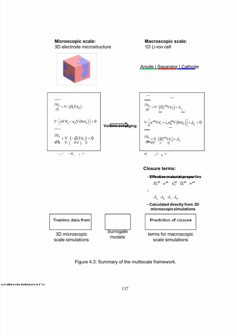
8/21/2019 zhangxc_1
http://slidepdf.com/reader/full/zhangxc1 154/178
Microscopic scale:
3D electrode microstructure
Macroscopic scale:
1D Li-ion cell
Anode | Separator | Cathode
( )22 2
c D c
t
∂= ∇ ⋅ ∇
∂ ( )2
eff 22 2 c
c D c J
t
∂= ∇ ⋅ ∇ +
∂
( )2 2ln 0D
V c κ κ ⎡ ⎤⎣ ⎦
∇ ⋅ ∇ + ∇ = ( )2
2 2
eff eff 2
ln 0D V
V c J κ ε κ ⎡ ⎤⎢ ⎥⎣ ⎦
∇ ⋅ ∇ + ∇ + =
( )1
eff 11 1 c
c D c J
t
∂= ∇ ⋅ ∇ +
∂( )1
1 10
c D c
t
∂+ ∇ ⋅ − ∇ =
∂
Volume averaging
11 V σ + =1 1 1σ =⋅ ⋅ =
Closure terms:
eff 2
Deff
κ eff D
κ eff
1D
eff σ
- Effective material properties
-
2c
J 2V
J 1
c J
1V J
- Calculated directly from 3D
microscopic simulations
3D microscopicscale simulations
Surrogate
models
terms for macroscopicscale simulations
Figure 4.3: Summary of the multiscale framework.
137
8/21/2019 zhangxc_1
http://slidepdf.com/reader/full/zhangxc1 155/178
138
To efficiently bridge microscopic and macroscopic scales, training data from 3D
microscopic simulations are used to construct surrogate models to rapidly and efficiently
predict closure terms in macroscopic scale simulations.
3. RESULTS AND DISCUSSION
3.1. Analysis of 3D Microscopic Simulation Results
Figure 4.4 shows the generated geometry for two phases. The specified
parameters for the microstructure are as follows: solid phase volume fraction is 0.6,
particle aspect ratio is 2, and equivalent particle radius is 5.34μm. There are 10 identical
ellipsoidal particles in the solid phase. The computational domain including both phases
is 10μm×10μm×10μm.
Figure 4.5 shows an example solution of Li ion concentration in both phases and
the reaction electric current at the interface. The boundary conditions at the bottom and
top boundaries are node values taken from a pseudo 2D model simulation solution at
z =170μm and z =180μm in the cathode at time t=2.173min. This indicates that the REV is
placed at z=175μm on the macroscopic mesh. In the pseudo 2D simulation set up, the cell
is discharged at 1C, the thickness for anode, separator, and cathode is 100, 25, and 100
μm, respectively. z axis goes from the anode to the cathode. The cathode starts from
z=125μm to z=225μm. It is shown in Figure 4.5 (a) that Li ion concentration accumulates
at the middle of the simulation domain for this particular case because the inserted Li
ions could not be diffused out quickly enough due to the intrinsically low diffusivity of
the solid active material phase. However, this is not the case for Li ion concentration
distribution in the liquid electrolyte, as shown in Figure 4.5 (b), because liquid electrolyte

8/21/2019 zhangxc_1
http://slidepdf.com/reader/full/zhangxc1 156/178
(a)
(c)
Figure 4.4: Generated microstructure: (a) liquid phase of electrolyte,
(b) solid phase of active material, and (c) the whole simulation
domain containin both hases.
139
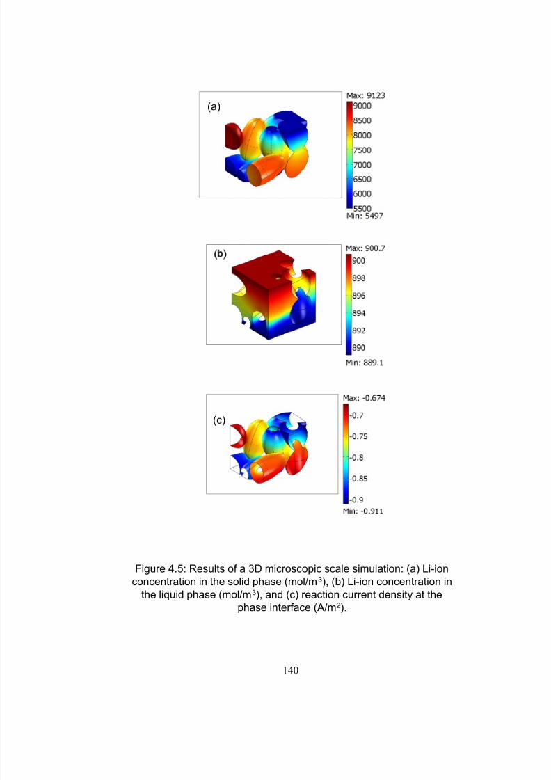
8/21/2019 zhangxc_1
http://slidepdf.com/reader/full/zhangxc1 157/178
(a)
(c)
Figure 4.5: Results of a 3D microscopic scale simulation: (a) Li-ion
concentration in the solid phase (mol/m3), (b) Li-ion concentration in
the liquid phase (mol/m3), and (c) reaction current density at the
phase interface (A/m2).
140
8/21/2019 zhangxc_1
http://slidepdf.com/reader/full/zhangxc1 158/178
141
has much higher diffusivity. Figure 4.5 (c) shows that the reaction current flux has the
same pattern of distribution as Li ion concentration in the solid phase. This is because the
reaction current flux depends on the surface overpotential whose distribution in this case
is dominantly determined by open circuit potential, a Li ion concentration dependent
material property of the solid active material.
Simulation results from the pseudo 2D model and detailed 3D microscopic model
are also compared. The REV is placed at macroscopic mesh node z=130μm. The
solutions from pseudo 2D model at z=125 μm and z=135 μm at t=2.173min are used as
boundary conditions for 3D microscopic modeling. Due to the stochastic feature of the
geometry modeling in detailed 3D microscopic modeling, three realizations of the
simulations are conducted, and the averaged results over these three realizations are used.
The comparison of specific interfacial area, reaction current density, and volumetric
reaction current from both pseudo 2D models and 3D microscopic models are shown in
Table 4.4. In Table 4.4, (normalized) reaction current density i of the 3D microscopic
model is calculated by integrating the local reaction current density over the interfacial
area and dividing the integral by the total area A of the interface
( )1 2 1 2, , , d A
i c c V V A
i A
=∫
. (34)
The volumetric reaction current V J is calculated by multiplying the interfacial area a
with the (normalized) reaction current density. Table 4.4 shows that simulation results
from three different realizations are consistent. It is also shown in Table 4.4 that the 3D
microscopic model gives large specific interfacial area for electrochemical reactions than
the pseudo 2D model. This is because ellipsoidal particles with aspect ratio 2 used in the

8/21/2019 zhangxc_1
http://slidepdf.com/reader/full/zhangxc1 159/178
o d e l s .
d 3 D
m i c r o s c o p i c
r o m p
s e u d o 2 D a n
s i m u l a t i o n r e s u l t s
. 4 : C o m p a r i s o n o f
T a b l e
142

8/21/2019 zhangxc_1
http://slidepdf.com/reader/full/zhangxc1 160/178
143
3D microscopic model have larger surface area than spherical particles with the same
volume used in the pseudo 2D model. Table 4.4 also shows that the (normalized) reaction
current density i of the 3D microscopic model is different from that of the pseudo 2D
model, because reaction current density is calculated directly using local variables in the
3D microscopic model and reaction current is calculated using volume averaged variables
in the pseudo 2D model, as pointed out in Equation (21). In Table 4.4, volumetric
reaction current from both models show different values. This implies that the source
terms in the macroscopic governing equations derived from the volume averaging
technique take different values from these two models. This difference eventually leads
to different solutions of the macroscopic governing equations. In other words, the closure
terms of volumetric reaction rate provided by pseudo 2D model and 3D microscopic
model generate different solutions of the macroscopic governing equations.
To study the effect of the number of particles in the cluster, simulations were also
conducted for 9 particle clusters. The simulation results are shown in Table 4.4. The
particles used here have the same volume as those used in the 10 particle cluster case. All
the other parameters (boundary conditions) used for the simulations are also the same as
those used in 10 particle cluster simulation. It is shown in Table 4.4 that simulation
results between 9 particle clusters and 10 particle clusters are consistent, which suggests
that using 10 particles in the cluster might be sufficient to represent the random
microstructure.
Normalized reaction current density from the pseudo 2D model and detailed 3D
microscopic model are further compared. The REV is placed at macroscopic mesh node
z=175μm. The temporal variations of (normalized) reaction current from two models are

8/21/2019 zhangxc_1
http://slidepdf.com/reader/full/zhangxc1 161/178
144
compared as shown in Figure 4.6(a). The curves from two models show completely
different temporal variation trends. To explain this discrepancy between two models, a
detailed investigation is carried out for microscopic 3D simulations at t=10.77min and
t=26.16min. Normalized reaction current densities are -0.78 A/m2
and -0.23 A/m2 for
t=10.77min and t=26.16min, respectively. Normalized reaction current density is actually
the averaged local reaction current density over the interfacial area. Local reaction
current densities at the interface for both time instants are shown in Figure 4.6(b) and (c).
It could be seen that the local current density distribution spans from -0.915 to -0.696
A/m
2
for t=10.77min, and it spans from -0.0125 to -1.024 A/m
2
for t=26.16min.
Therefore, different averaged local reaction current densities for these two time instants
are expected. To further understand the different distribution range of local current
density for these two time instants, one needs to start from the plateaus in the open circuit
potential profile caused by material phase changes. Figure 4.6(d) shows the ranges of
open circuit potential distribution for both solutions at these two time instants. Though
t=10.77min solution has wider distribution of Li ion concentration in solid phase than
t=26.16min solution does, t=10.77min solutions spans a smaller range of open circuit
potential than t=26.16min solutions does because t=10.77min solution locates around the
plateau region of open circuit potential where phases change is experienced by the active
material. A smaller range of open circuit potential results in a smaller range of surface
over potential and local reaction current density for t=10.77min solution. Therefore, a big
difference is observed in normalized current densities shown in Figure 4.6(a). To
summarize, the effect of local variable distribution is very important for the normalized
reaction current density. The 3D microscopic model is capable of revealing the local

8/21/2019 zhangxc_1
http://slidepdf.com/reader/full/zhangxc1 162/178
(a)
(b) (c)
(d)
t=10.77min t=26.16min
Figure 4.6: Comparison of (normalized) reaction current density: (a) the
temporal variation for pseudo 2D and 3D microscopic models, (b) distribution
of reaction current density (A/m2) at t=10.77min by 3D microscopic model, and
.
microscopic model.
145

8/21/2019 zhangxc_1
http://slidepdf.com/reader/full/zhangxc1 163/178
146
distribution of variables. This demonstrates the importance of conducting 3D microscopic
modeling.
3.2. Effective Material Property Calculations
The closure terms of effective material properties are calculated directly from 3D
microscopic simulations. The calculated results of the ratio between effective and bulk
(intrinsic) transport properties are shown in Table 4.5. Since effective transport properties
eff D2 , eff κ , eff
Dκ , eff
D1 , and eff σ are all defined in the same manner (2 2 2 2
eff D c D c∇ = ∇ ,
2 2
eff V V κ κ ∇ = ∇ , ( ) ( )2 2
ln lneff
D Dc cκ κ ∇ = ∇ , 1 1 1 1
eff D c D c∇ = ∇ , 1 1
eff V V σ σ ∇ = ∇ ), they should share the same
value of the ratio between effective and bulk properties. To calculate the effective
materials properties, the generated 3D microstructure is scaled to a cube of 1m×1m×1m,
and Poisson’s equation ( ) 0 D c∇ ⋅ ∇ = is solved with top and bottom boundary specified as
3( 1m) 1 mol/mc z = = , and 3
( 0m) 0 mol/mc z = = , and other boundaries specified as symmetric. A
bulk diffusion coefficient bulk 21 m /s D = is used. The effective diffusivity is calculated as
( )[ ] ( )
bulk
( 1m)eff
d
1m 1m ( 1m) ( 0m) / 1m 0m
A z
D c A
Dc z c z
=∇
=× ⋅ = − = −
∫.
(35)
The ratio between the effective and bulk diffusivity is
( )eff
bulk 2
( 1)
1d
1mol/m A z
Dc A
D=
⎡ ⎤⎢ ⎥= ∇⎢ ⎥⎣ ⎦
∫ . (36)
For each of the three realizations of the specified geometry, this calculation is carried out
three times by assigning the concentration difference boundary conditions along x, y and
z directions respectively. Therefore, nine simulation results for this ratio between the
effective and bulk diffusivity are obtained. The averaged value and deviation are
calculated. Table 4.5 presents the ratios between effective and bulk (intrinsic) transport

8/21/2019 zhangxc_1
http://slidepdf.com/reader/full/zhangxc1 164/178
Bruggeman’s
Equation
3D microscopic model
Average Deviation (%)
Solid phase 0.465 0.224 5.2
Liquid phase 0.253 0.276 2.5
Table 4.5: Ratio between effective and bulk (intrinsic) transport
properties.
147

8/21/2019 zhangxc_1
http://slidepdf.com/reader/full/zhangxc1 165/178
148
properties in solid and liquid phase from the conventional Bruggeman’s equation and 3D
microscopic simulations. It could be seen that 3D microscopic simulations give very
different ratios those given by Bruggeman’s equation. It should be pointed out that the
effective transport properties for the solid phase of the microstructure depend a lot on the
overlapping specified between the particles. It was mentioned that a coefficient of 1.1
was used to multiply the semi-axis of ellipsoids to create an artificial overlapping for a
continuous conduction path. A better approach to determine the overlapping coefficient
would be using experimentally measured effective and bulk (intrinsic) conductivity and
3D numerical simulations of microstructure for an iterative fitting.
3.3. Surrogate Model Construction for Reaction Current Density
3D microscopic scale simulation results of normalized reaction current density on
317 sampling points in total are used to construct 2nd
order polynomial response surface,
kriging and radial basis neural network models. The error measures used for evaluating
the constructed models are summarized in Table 4.6. PRESS root mean square (RMS)
error for all three models is less than 8%. 2adj R for 2
nd order polynomial response surface
is 0.97, a value very close to one. The error measures suggest that the surrogate models
constructed have sufficient accuracy for predicting the objective function, normalized
reaction current. Among these three models, kriging has the smallest PRESS RMS, and
will be used for further analysis.
To further evaluate the performance of the constructed kriging model, prediction
results by the kriging model on 21 testing points are compared with the actual 3D
microscopic simulation results. These 21 testing points are sampled using the Latin
hypercube filling method to make sure that they do not overlap with any training points

8/21/2019 zhangxc_1
http://slidepdf.com/reader/full/zhangxc1 166/178
urroga e mo e r g ng
(normalized)
PRESS RMS0.030 0.014 0.074
R2adj 0.97 - -
Table 4.6: Evaluation of the constructed surrogate models.
149

8/21/2019 zhangxc_1
http://slidepdf.com/reader/full/zhangxc1 167/178
150
used for surrogate model construction. The error of prediction by the kriging model on
these 21 testing points is summarized in Figure 4.7. Figure 4.7 gives the histogram of the
prediction error for all 21 points. The horizontal axis is the value of prediction error, and
the vertical axis is the number of points (or cases) where the error falls into the range
indicated by the bars. As shown in Figure 4.7, most of the testing points have prediction
error less than 10% except for 3 points which are found to be close to boundaries of the
design space. 16 points have prediction error less than 4.5%. Therefore, the constructed
kriging model generally gives good prediction of normalized reaction current density
except for some regions close to boundaries. This lack of prediction accuracy in regions
close to boundaries can be remedied by using more training points chosen from the
boundary regions. The implication of poor prediction for regions close to boundaries is
that the construct surrogate model does not accurately predict the current density for
extreme cases of very high discharge rates. The constructed kriging model is generally
adequate to deal with moderate discharge rates in the multiscale modeling of batteries.
Global sensitivity analysis, which is often used to study the importance of design
variables, is conducted to quantify variation of the objective function (normalized
reaction current density) caused by the design variables: concentration, electric potential
and their gradients in both solid and liquid phases. The importance of design variables is
presented by the main factor and total effect indices [30]. The main factor is the fraction
of the total variance of the objective function contributed by a particular variable in
isolation, while the total effect includes contribution of all partial variances in which the
variable of interest is involved (basically by considering those interaction terms in the
response surface approximation). The results of calculated main factor and total effect

8/21/2019 zhangxc_1
http://slidepdf.com/reader/full/zhangxc1 168/178
Figure 4.7: Histogram of surrogate model prediction errors on 21
testing points.
151

8/21/2019 zhangxc_1
http://slidepdf.com/reader/full/zhangxc1 169/178
152
indices are shown in Table 4.7. It can be seen that the gradient of variables contribute
very little to the variable of the objective function. This is because the ranges of the
gradients of the concentration and electric potential variables are chosen based on their
distribution on the microscopic scale, while the ranges of the variables themselves are
chosen based on their distribution on the macroscopic scale. Table 4.7 also shows that the
contribution of variables in the solid phase is larger than those variables in the liquid
phase. This is because the solid phase variables dominantly affect the surface
overpotential of the electrochemical reactions.
In summary, the constructed surrogate model is capable of predicting the closure
term of normalized reaction current density, and will be used for scale bridging in the
multiscale modeling framework.
4. CONCLUSIONS
A multiscale framework was proposed to include the electrode microstructure
information in battery scale modeling. The resulting closure terms for macroscopic scale
governing equations derived from the volume averaging technique were calculated
directly from 3D microscopic scale simulations of microstructure consisting of multiple
(ellipsoidal) electrode active material particles and liquid electrolyte phase. Comparison
of simulation results from 3D microscopic particle clusters and the conventional pseudo
2D models showed that 3D microscopic model (1) gives larger interfacial area for
electrochemical reaction; (2) generates different normalized reaction current density (a
closure term for the macroscopic scale model) because the 3D microscopic model reveals
the local distribution of variables. The calculated effective material properties also

8/21/2019 zhangxc_1
http://slidepdf.com/reader/full/zhangxc1 170/178
k r i g i n g m o d e l .
e s c a l c u l a t e d f r o m
b a l s e n s i t i v i t y i n d i c
T a b l e 4 . 7 : G l o
153

8/21/2019 zhangxc_1
http://slidepdf.com/reader/full/zhangxc1 171/178
154
showed very different values from those by the conventional Bruggeman’s equation.
These suggest the importance and necessity of conducting 3D microscopic modeling and
incorporating it into battery scale modeling by the multiscale framework proposed. To
efficiently exchange the information between microscopic and macroscopic scales, a
surrogate-based approach was proposed for scale bridging. Surrogate models were
constructed based on 3D microscopic scale simulation results on sampling points chosen
by design of experiments. It was shown that the constructed surrogate models fit the
training data of (normalized) reaction current density very well, and they can be used for
bridging microscopic and macroscopic scale simulations.

8/21/2019 zhangxc_1
http://slidepdf.com/reader/full/zhangxc1 172/178
155
BIBLIOGRAPHY
1. J. Newman and K. Thomas-Alyea, Electrochemical Systems (third edition), John
Wiley & Sons, New Jersey, 2004.
2. Y. Chen and J.W. Evans, Three-Dimensional Thermal Modeling of Lithium-
Polymer Batteries under Galvanostatic Discharge and Dynamic Power Profile,
Journal of the Electrochemical Society, 141, 2947-2955 (1994).
3. X. Zhang, W. Shyy, and A. M. Sastry, Numerical Simulation of Intercalation-Induced Stress in Li-Ion Battery Electrode Particles, Journal of the
Electrochemical Society, 154, A910-A916 (2007).
4. M. W. Verbrugge and R. S. Conell, Electrochemical and ThermalCharacterization of Battery Modules Commensurate with Electric Vehicle
Integration, Journal of The Electrochemical Society, 149, A45-A53 (2002).
5. B. Y. Liaw, G. Nagasubramanian, R. G. Jungst, and D. H. Doughty, Modeling ofLithium Ion Cells – A Simple Equivalent-Circuit Model Approach, Solid State
Ionics, 175, 835-839 (2004).
6. P. L. Moss, G. Au, E. J. Plichta, and J. P. Zheng, An Electrical Circuit forModeling the Dynamic Response of Li-Ion Polymer Batteries, Journal of The
Electrochemical Society, 155, A986-A994 (2008).
7. J. Newman and W. Tiedemann, Porous-Electrode Theory with Battery
Applications, AIChE Journal, 21, 25-41 (1975).
8. M. Doyle, T. F. Fuller, and J. Newman, Modeling of Galvanostatic Charge andDischarge of the Lithium Polymer Insertion Cell, Journal of The Electrochemical
Society, 140, 1526-1533 (1993) .
9. T. F. Fuller, M. Doyle, and J. Newman, Simulation and Optimization of the DualLithium Ion Insertion Cell, Journal of The Electrochemical Society, 141, 1-10
(1994).
10. K. Smith and C.-Y. Wang, Solid-State Diffusion Limitations on Pulse Operationof a Lithium Ion Cell for Hybrid Electric Vehicles, Journal of Power Sources,
161, 628–639 (2006).
11. G. Sikha, B. N. Popov, and R. E. White, Effect of Porosity on the Capacity Fade
of a Lithium-Ion Battery – Theory, Journal of The Electrochemical Society, 151,
A1104-A1114 (2004).
12. X. Zhang, A. M. Sastry, and W. Shyy, Intercalation-Induced Stress and Heat
Generation within Single Lithium-Ion Battery Cathode Particles, Journal of The
Electrochemical Society, 155, A542-A552 (2008).
8/21/2019 zhangxc_1
http://slidepdf.com/reader/full/zhangxc1 173/178
156
13. C.-W. Wang and A. M. Sastry, Mesoscale Modeling of a Li-Ion Polymer Cell,
Journal of The Electrochemical Society, 154, A1035-A1047 (2007).
14. W. R. McKinnon and R. R. Haering, Physical Mechanisms of Intercalation. In
Modern Aspects of Electrochemistry, No. 15, edited by Ralph E. White et al.
Plenum Press, New York (1983).
15. K. E. Thomas, and J. Newman, Thermal Modeling of Porous Insertion Electrodes,
Journal of the Electrochemical Society, 150, A176-A192 (2003).
16. Y. Chen and J. W. Evans, Heat Transfer Phenomena in Lithium/Polymer-Electrolyte Batteries for Electric Vehicle Application, Journal of The
Electrochemical Society, 140, 1833-1838 (1993).
17. S. C. Chen, C. C. Wan, and Y. Y. Wang, Thermal analysis of lithium-ion
batteries, Journal of Power Sources 140, 111–124 (2005).
18. W. Shyy, S. S. Thakur, H. Ouyang, J. Liu, and E. Blosch, Computational
Techniques for Complex Transport Phenomena, Cambridge, 1997.
19. U. Hornung (editor), Homogenization and Porous Media, Springer, New York,
1997.
20. E. Sanchez-Palencia, Non-Homogeneous Media and Vibration Theory, edited by
J. Ehlers et al, Lecture Notes in Physics, Springer-Verlag, New York, 1980.
21. E. Sozer and W. Shyy, Multi-scale Thermo-fluid Transport in Porous Media,
International Journal of Numerical Methods for Heat & Fluid Flow, 18(7/8) 883-
899 (2008).
22. P. D. Vidts and R. E. White, Governing Equations for Transport in Porous
Electrodes, Journal of The Electrochemical Society, 144, 1343-1353 (1997).
23. W. B. Gu, C. Y. Wang, and B. Y. Liaw, Micro-Macroscopic Coupled Modeling
of Batteries and Fuel Cells, Journal of the Electrochemical Society, 145, 3407-
3418 (1998).
24. K. K. Patel, J. M. Paulsen, and J. Desilvestro, Numerical Simulation of Porous
Networks in Relation to Battery Electrodes and Separators, Journal of Power
Sources 122, 144–152 (2003).
25. R. J. M. Smit, W. A. M. Brekelmans, and H. E. H. Meijer, Prediction of the
Mechanical Behavior of Nonlinear Heterogeneous Systems by Multi-Level Finite
Element Modeling, Computer Methods in Applied Mechanics and Engineering,
155, 181-192 (1998).

8/21/2019 zhangxc_1
http://slidepdf.com/reader/full/zhangxc1 174/178
157
26. V. Kouznetsova, W. A. M. Brekelmans, and F. P. T. Baaijens, An Approach toMicro-Macro Modeling of Heterogeneous Materials, Computational Mechanics
27, 37-48 (2001).
27. W. E, B. Engquist, X. Li, W. Ren, and E. Vanden-Eijnden, HeterogeneousMultiscale Methods: a Review, Communications in Computational Physics, 2,
367-450 (2007).
28. L. Tan and N. Zabaras, Multiscale Modeling of Alloy Solidification Using a
Database Approach, Journal of Computational Physics 227, 728–754 (2007).
29. O. Rohrle, J. B. Davidson, and A. J. Pullan, Bridging Scales: A Three-
Dimensional Electromechanical Finite Element Model of Skeletal Muscle, SIAM
Journal on Scientific Computing, 30, 2882–2904 (2008).
30. N. V. Queipo, R. T. Haftka, W. Shyy, T. Goel, R. Vaidyanathan, and P. K.
Tucker, Surrogate-based Analysis and Optimization, Progress in AerospaceSciences, 41, 1-28 (2005).
31. A. Donev, F. H. Stillinger, and S. Torquato, Neighbor List Collision-Driven
Molecular Dynamics Simulation for Nonspherical Particles. I. Algorithmic
Details II. Applications to Ellipses and Ellipsoids, Journal of Computational
Physics, 202, 737-764 (part I) and 765-793 (part II) (2005).
32. J. I. Madsen, W. Shyy and R. T. Haftka, Response Surface Techniques for
Diffuser Shape Optimization, AIAA Journal, 38, 1512-1518 (2000).
33. T. Goel, R. Vaidyanathan, R. T. Haftka, W. Shyy, N. V. Queipo, and K. Tucker,
Response Surface Approximation of Pareto Optimal Front in Multi-ObjectiveOptimization, Computer Methods in Applied Mechanics and Engineering, 196,
879–893 (2007).
34. R. H. Myers, and D. C. Montgomery, Response Surface Methodology: Processand Product Optimization Using Designed Experiments, pp. 17-48, John Wiley &
Sons Inc: New York, 1995.

8/21/2019 zhangxc_1
http://slidepdf.com/reader/full/zhangxc1 175/178
158
CHAPTER V
CONCLUSIONS AND FUTURE WORK
To improve Li-ion battery performance for application in electrifying automotive
drivetrains, this study focuses on (1) improving calendar life by reducing performance
degradation due to stress-induced electrode particle fracture and heat generation through
modeling and numerical simulations, and (2) creating models including electrode
materials microstructural information for computer simulations that can lead to
optimizing battery design for improved energy output per unit volume and mass.
An intercalation-induced stress model with the analogy to thermal stress modeling
was proposed to determine localized intercalation-induced stress in electrode particles.
Intercalation-induced stress was first calculated within ellipsoidal electrode particles with
a constant diffusion flux assumed at the particle surface. It was found that internal stress
gradients significantly enhance diffusion. Simulation results suggest that it is desirable to
synthesize electrode particles with smaller sizes and larger aspect ratios, to reduce
intercalation-induced stress during cycling of lithium-ion batteries.
Stress and heat generation were modeled for single ellipsoidal particles under
potentiodynamic control, in which case the flux at particle surface is determined by
electrochemical kinetics, Butler-Volmer equation. It was found that Li-ion concentration,
surface flux, and intercalation-induced stress are highly correlated through the diffusion
process, electrochemical kinetics and the intercalation-induced lattice expansion. The two

8/21/2019 zhangxc_1
http://slidepdf.com/reader/full/zhangxc1 176/178
159
peaks observed in the flux and stress generation plots were attributable to intrinsic
material properties (two plateaus in the OCP) of the material studied (LiMn2O4) and the
applied potential. The heat of mixing was found to be negligible (two orders of
magnitude smaller than the other two sources) and resistive heat was identified as the
heat generation source of greatest importance. To systematically investigate how
intercalation-induced stress and resistive heat generation are affected by electrode particle
geometric shape and cycling rate, a surrogate-based analysis was conducted. It was
shown that smaller sizes and larger aspect ratios of (prolate) particles reduce the heat and
stress generation inside electrode particles.
A multiscale framework was proposed to include the electrode microstructure
information in battery scale modeling. The resulting closure terms for macroscopic scale
governing equations derived from the volume averaging technique were calculated
directly from 3D microscopic scale simulations of microstructure consisting of multiple
(ellipsoidal) electrode particles and liquid electrolyte. Comparison of simulation results
from 3D microscopic particle clusters and the conventional pseudo 2D models showed
that the 3D microscopic model (1) gives larger interfacial area for electrochemical
reaction; (2) generates different normalized reaction current density (a closure term for
the macroscopic scale model) because the 3D microscopic model reveals the local
distribution of variables. This suggests the importance and necessity of conducting 3D
microscopic modeling and incorporating it into battery scale modeling by the multiscale
framework proposed. To efficiently exchange the information between microscopic and
macroscopic scales, a surrogate-based approach was proposed for scale bridging.
Surrogate models were constructed based on 3D microscopic scale simulation results on

8/21/2019 zhangxc_1
http://slidepdf.com/reader/full/zhangxc1 177/178
160
sampling points chosen by design of experiments. The inputs for surrogate models are
boundary conditions for 3D microscopic scale simulations taken from the nodal values of
macroscopic scale simulations. The output is the (normalized) reaction current density for
closure term in macroscopic scale simulations. It was shown that the constructed
surrogate models fit the training data very well and give good prediction of the closure
term modeled, reaction current density.
Future work is proposed in the following areas:
• Use the constructed surrogate models for the closure term of volumetric reaction
rate to complete the multiscale modeling framework.
• Incorporate material phase change in the diffusion and intercalation-induced
stress modeling. It is well know that electrode active materials undergo phase
change during intercalation and deintercalation. Different phases of the material
have different diffusion coefficient and structural properties. It is important to
include this phase change information into models.
• Include stress analysis and heat generation and transfer modules into the proposed
multiscale modeling framework. In this study, stress and heat generation were
studied for single electrode particles. With the understanding of stress and heat
generation mechanisms inside single particles, it is necessary to analyze stress and
heat transfer on the cell scale to further understand the effect of electrode
microstructure on stress generation and heat generation and transfer.
• Further explore the effect of 3D microstructure on battery performance. A fixed
set of microstructure characteristic parameters were used in this study. It is
necessary to improve the robustness of the geometry modeling and meshing

8/21/2019 zhangxc_1
http://slidepdf.com/reader/full/zhangxc1 178/178
process so that it is feasible to fully explore the effect of the 3D microstructure of
electrode materials.
• Further explore the application of the surrogate-based approach for modeling and
optimization. Surrogate models are reduced order models with adequate fidelity.
They predict the objective functions efficiently compared to physics-based
models. For example, surrogate models can be potentially used for battery control
algorithms where rapid prediction of state variables is required. Furthermore,
surrogate models can also be used for design optimization purpose. Design
adjustable parameters for a Li-ion cell include electrode thickness, volume
fractions of active material, conductive additives, and electrolyte in the electrode,
electrode particle size separator thickness and other adjustable material


