[email protected] STAT151: Introduction to Statistical Theory Term I, 2015-2016 Yang Zhenlin

[email protected]://www.mysmu.edu/faculty/zlyang/

STAT151: Introduction to Statistical Theory

Term I, 2015-2016

Yang Zhenlin

STAT151, Term I 2015-16 © Zhenlin Yang, SMU

Chapter 1

Course Contents

2

Confidence Intervals

Testing Statistical Hypotheses Course Outline

This course serves as an introduction to basic statistical theory for students who intend to pursue a quantitative major at SMU such as Applied Statistics, Actuarial Science, Economics, Finance, Marketing, Management, etc. Students are expected to have some basic knowledge in probability and statistics and to be mathematically oriented or at the very least, be interested in mathematics. Major topics include:

This course serves as an introduction to basic statistical theory for students who intend to pursue a quantitative major at SMU such as Applied Statistics, Actuarial Science, Economics, Finance, Marketing, Management, etc. Students are expected to have some basic knowledge in probability and statistics and to be mathematically oriented or at the very least, be interested in mathematics. Major topics include:

Distributions and Conditional Distributions

Point Estimations

Probability and Conditional Probability


Chapter 1

In any scientific study of a physical phenomenon, it is desirable to have a mathematical model that makes it possible to describe or predict the observed value of some characteristic of interest.

The physical situations may be deterministic, such as the speed of a falling object in a vacuum, travel distance of an airplane in certain time period when the speed is set to a constant, etc., or may be nondeterministic, such as the outcome of tossing a coin, the lifetime of a light bulb, etc.

This course concerns the latter situation: to provide a probability model so as to facilitate the “statistical inference” for the nondeterministic situation.

Chapter 1: Probability

3


Chapter 1

Concepts of probability have been around for thousands of years, but probability theory did not arise as a branch of mathematics until the mid-seventeenth century.

In the mid-seventeenth century, a simple question directed to Blaise Pascal by a nobleman sparked the birth of probability theory.

Chevalier de Méré gambled frequently to increase his wealth. He bet on a roll of a die that at least one 6 would appear during a total of 4 rolls, and was more successful than not with this game of chance.

Tired of his approach, he decided to change the game. He bet on a roll of two dice that he would get at least one double 6, on twenty-four rolls of two dice. Soon he realized that his old approach to the game resulted in more money. He asked his friend Blaise Pascal why his new approach was not as profitable.

Pascal worked through the problem and found that the probability of winning using the new approach was only 49.14 percent compared to 51.77 percent using the old approach.

Brief History

4


Chapter 1

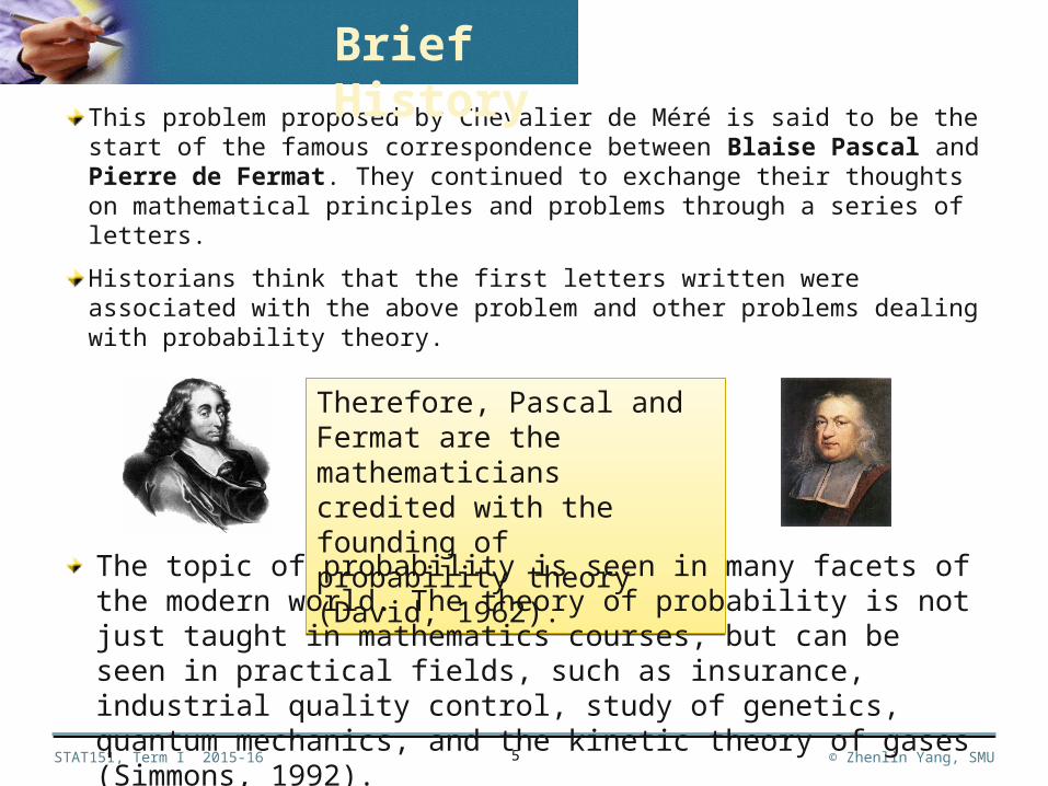
This problem proposed by Chevalier de Méré is said to be the start of the famous correspondence between Blaise Pascal and Pierre de Fermat. They continued to exchange their thoughts on mathematical principles and problems through a series of letters.

Historians think that the first letters written were associated with the above problem and other problems dealing with probability theory.

5

Therefore, Pascal and Fermat are the mathematicians credited with the founding of probability theory (David, 1962).

Therefore, Pascal and Fermat are the mathematicians credited with the founding of probability theory (David, 1962).

The topic of probability is seen in many facets of the modern world. The theory of probability is not just taught in mathematics courses, but can be seen in practical fields, such as insurance, industrial quality control, study of genetics, quantum mechanics, and the kinetic theory of gases (Simmons, 1992).

Brief History


Chapter 1

6

Sample Space and Events

Basic Set Algebra

Definition of Probability

Conditional Probability

Rules for Calculating Probabilities

Probability Trees

Counting Techniques

Learning Objectives


Chapter 1

Some fundamental concepts are important to the learning of probability theory:

An experiment refers to the process of obtaining an observed result of some phenomenon.

A trial refers to a run of an experiment.

An outcome refers to the observed result.

The set of all possible outcomes of an experiment is called the sample space, denoted by S.

Note: One and only one of the possible outcomes will occur on any given trial of the experiment.

7



Chapter 1

Example 1.1 An experiment consists of tossing two coins, and the observed face of each coin is of interest. The set of possible outcomes is represented by the sample space:

S = {HH, HT, TH, TT}, where H=Head, and T=Tail.

Example 1.2. Suppose in Example 1.1, we are instead interested in the total number of heads obtained from the two coins. An appropriate sample space could then be defined as

S = {0, 1, 2}.

Thus, a different sample space may be appropriate for the same experiment, depending on the characteristic of interest.

8



Chapter 1

More fundamental concepts:

A sample space S is said to be finite if it consists of a finite number of elements, say S = {e1, e2, . . . , eN}, and countably infinite if its outcomes can be put into a one-to-one correspondence with the positive integers 1, 2, 3, . . .

If a sample space S is either finite or countably infinite, then it is called a discrete sample space; If the outcomes can assume any value in some interval of real numbers then the sample space is called a continuous sample space.

Note: the sample spaces in Examples 1.1 and 1.2 are discrete.

Example 1.3. If a coin is tossed repeatedly until a head occurs, then a natural sample space is

S = {H, TH, TTH, TTTH, . . . }.9



Chapter 1

If in Example 1.3 one is interested in the number of tosses required to obtain a head, then a possible sample space would be the set of all positive integers, i.e., S = {1, 2, 3, . . . }.

Clearly these are countable and infinite sample spaces.

10


Event. Any subset A of the sample space S is defined as an event. If the outcome of an experiment is contained in A, then we say event A has occurred in this experiment.

Event. Any subset A of the sample space S is defined as an event. If the outcome of an experiment is contained in A, then we say event A has occurred in this experiment.

Example 1.4. A light bulb is placed in service and the time of operation (in hours) until it burns out is measured, then the sample space consists of all nonnegative real numbers, i.e.,

S = {t | 0 ≤ t < ∞},

which is a continuous sample space.


Chapter 1

A set is a collection of distinct objects. Sets usually are designated by capital letters, A, B, C, . . . , or subscripted letters A1, A2, A3, . . .

Individual objects in a set A are called elements.

In the context of probability, the sets are called events and the elements are called outcomes.

Universal set S is the set of all elements under consideration. In probability application it is called the sample space.

Empty set or null set, denoted by , is the set that contains no element. In probability, it is empty event.

11

Set Algebra

The study of probability models requires a familiarity of basic notations of set theory.


Chapter 1

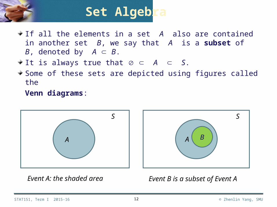
If all the elements in a set A also are contained in another set B, we say that A is a subset of B, denoted by A B.

It is always true that A S.

Some of these sets are depicted using figures called the

Venn diagrams:

12

S S

BA A

Event A: the shaded area Event B is a subset of Event A

Set Algebra


Chapter 1

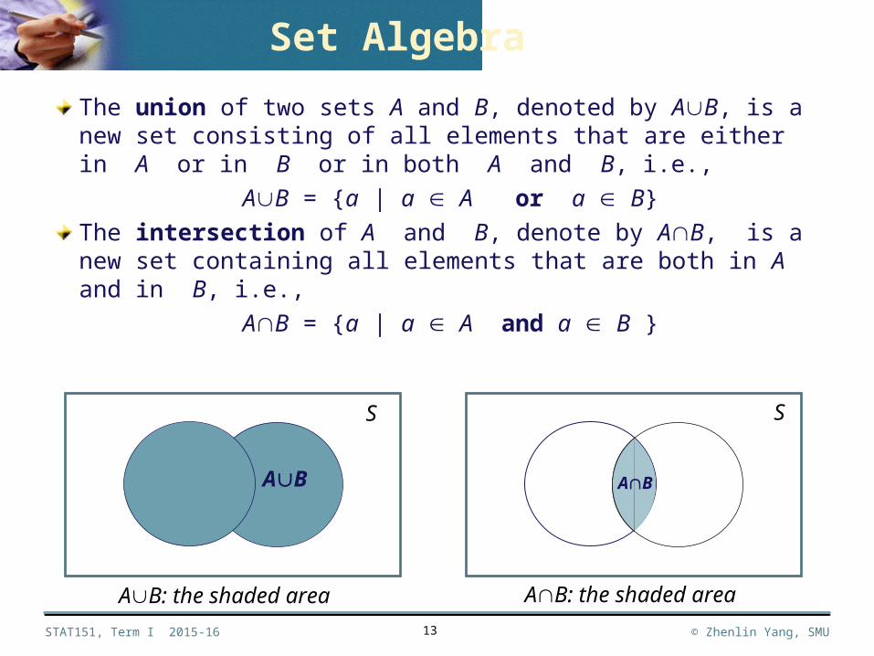
The union of two sets A and B, denoted by AB, is a new set consisting of all elements that are either in A or in B or in both A and B, i.e.,

AB = {a | a A or a B}

The intersection of A and B, denote by AB, is a new set containing all elements that are both in A and in B, i.e.,

AB = {a | a A and a B }

13

S

S

ABAB

AB: the shaded area AB: the shaded area

Set Algebra


Chapter 1

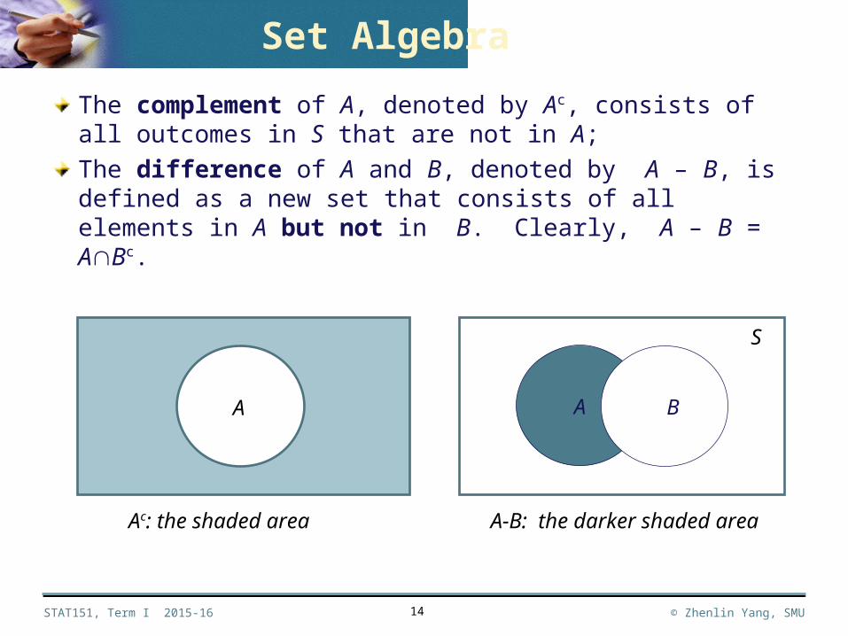
The complement of A, denoted by Ac, consists of all outcomes in S that are not in A;

The difference of A and B, denoted by A – B, is defined as a new set that consists of all elements in A but not in B. Clearly, A – B = ABc.

14

Ac: the shaded area

A

S

A B

A-B: the darker shaded area

Set Algebra


Chapter 1

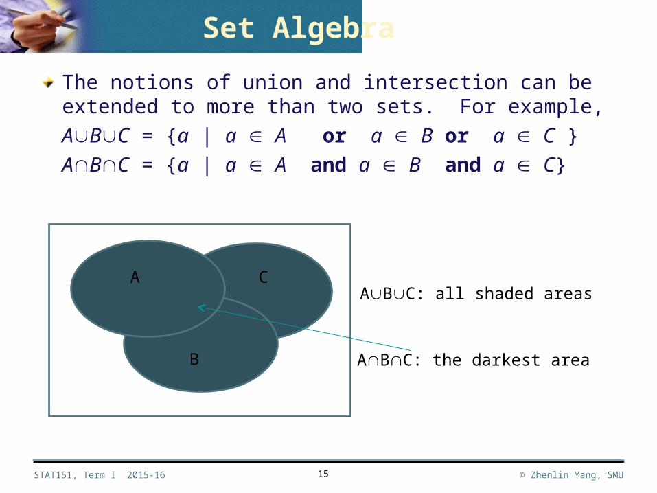
The notions of union and intersection can be extended to more than two sets. For example,

ABC = {a | a A or a B or a C }

ABC = {a | a A and a B and a C}

15

A C

B

ABC: all shaded areas

ABC: the darkest area

Set Algebra


Chapter 1

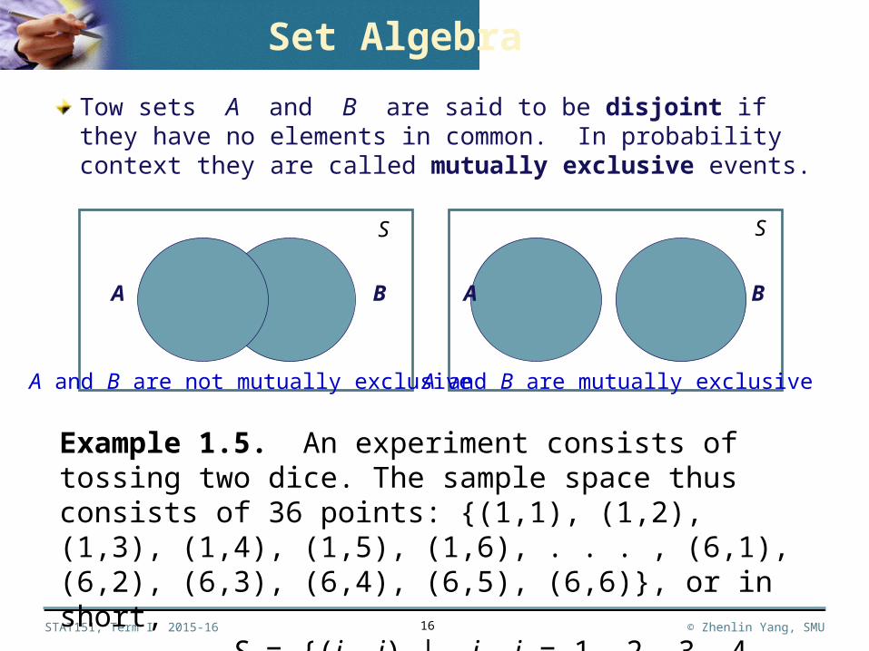
Tow sets A and B are said to be disjoint if they have no elements in common. In probability context they are called mutually exclusive events.

16

Example 1.5. An experiment consists of tossing two dice. The sample space thus consists of 36 points: {(1,1), (1,2), (1,3), (1,4), (1,5), (1,6), . . . , (6,1), (6,2), (6,3), (6,4), (6,5), (6,6)}, or in short,

S = {(i, j) | i, j = 1, 2, 3, 4, 5, 6}

Set Algebra

A B

S

A and B are mutually exclusive

S

A B

A and B are not mutually exclusive


Chapter 1

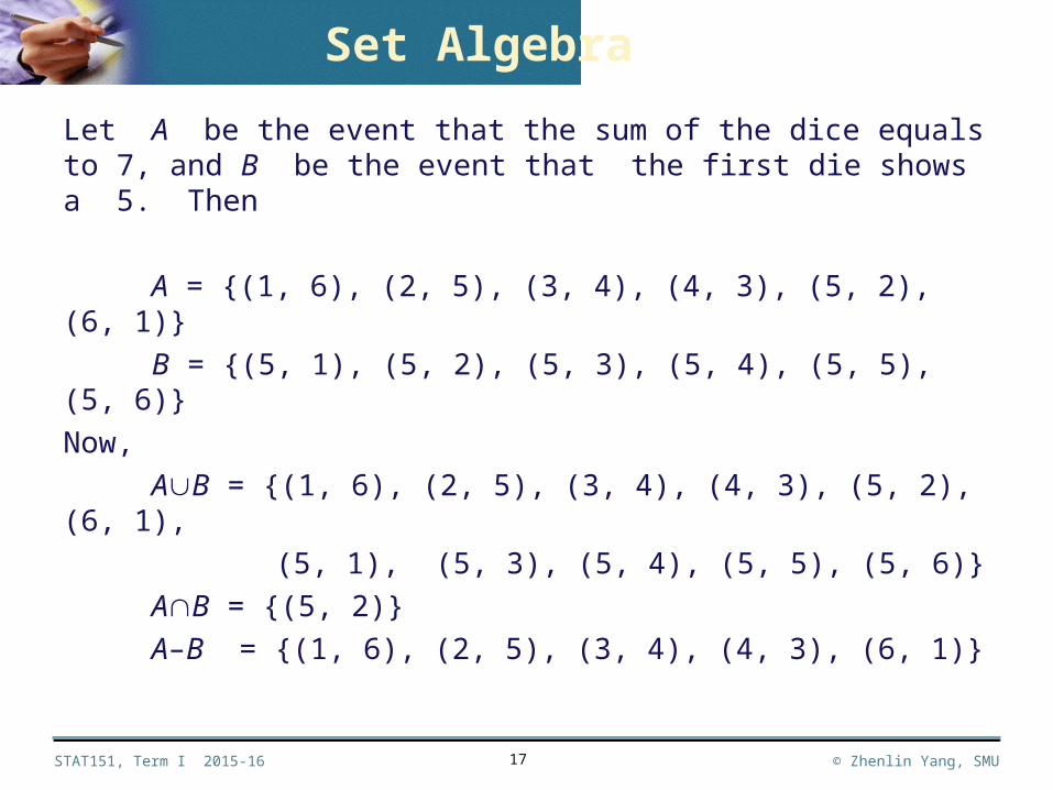
Let A be the event that the sum of the dice equals to 7, and B be the event that the first die shows a 5. Then

A = {(1, 6), (2, 5), (3, 4), (4, 3), (5, 2), (6, 1)}

B = {(5, 1), (5, 2), (5, 3), (5, 4), (5, 5), (5, 6)}

Now,

AB = {(1, 6), (2, 5), (3, 4), (4, 3), (5, 2), (6, 1),

(5, 1), (5, 3), (5, 4), (5, 5), (5, 6)}

AB = {(5, 2)}

A–B = {(1, 6), (2, 5), (3, 4), (4, 3), (6, 1)}

17

Set Algebra


Chapter 1

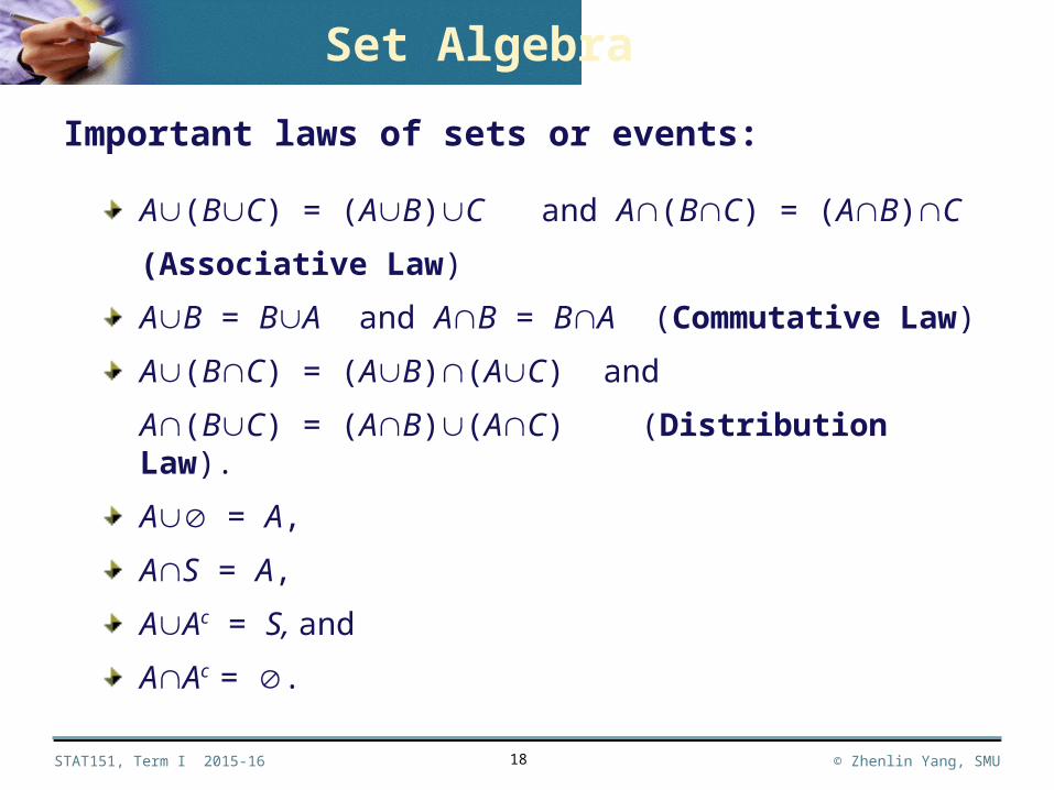
A(BC) = (AB)C and A(BC) = (AB)C

(Associative Law)

AB = BA and AB = BA (Commutative Law)

A(BC) = (AB)(AC) and

A(BC) = (AB)(AC) (Distribution Law).

A = A,

AS = A,

AAc = S, and

AAc = .

18

Set Algebra

Important laws of sets or events:


Chapter 1

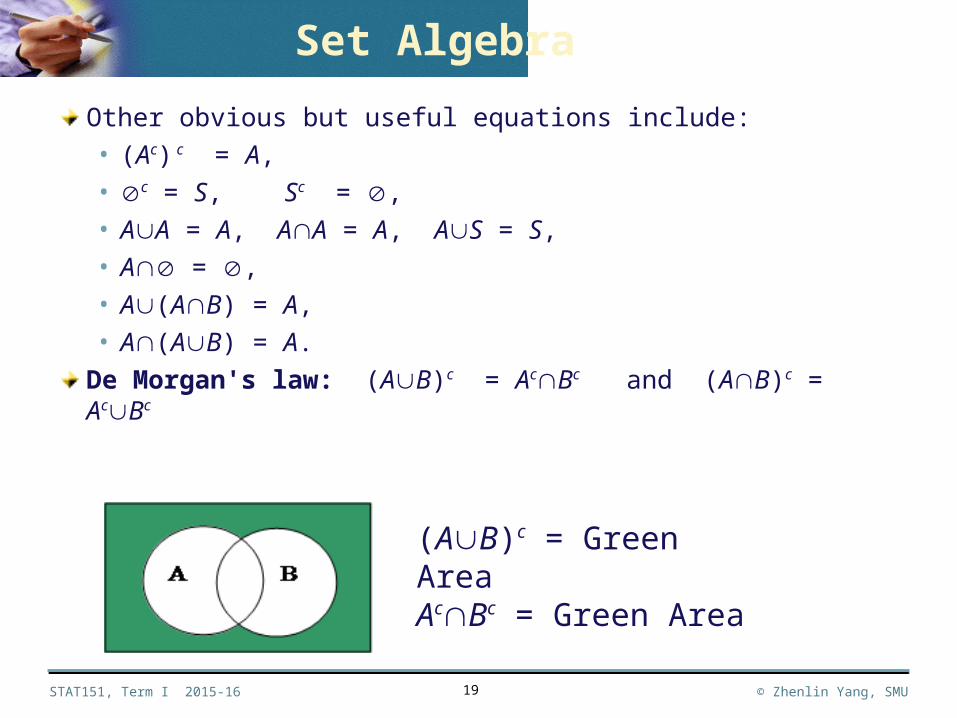
Other obvious but useful equations include:

• (Ac) c = A,

• c = S, Sc = ,

• AA = A, AA = A, AS = S,

• A = ,

• A(AB) = A,

• A(AB) = A.

De Morgan's law: (AB)c = AcBc and (AB)c = AcBc

19

(AB)c = Green Area

AcBc = Green Area

Set Algebra


Chapter 1

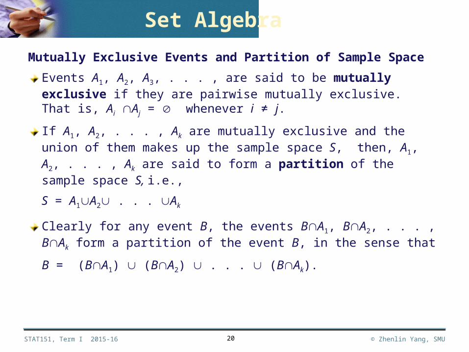
Mutually Exclusive Events and Partition of Sample Space

Events A1, A2, A3, . . . , are said to be mutually exclusive if they are pairwise mutually exclusive. That is, Ai Aj = whenever i ≠ j.

If A1, A2, . . . , Ak are mutually exclusive and the union of them makes up the sample space S, then, A1, A2, . . . , Ak are said to form a partition of the sample space S, i.e.,

S = A1A2 . . . Ak

Clearly for any event B, the events BA1, BA2, . . . , BAk form a partition of the event B, in the sense that

B = (BA1) (BA2) . . . (BAk).

20

Set Algebra


Chapter 1

21

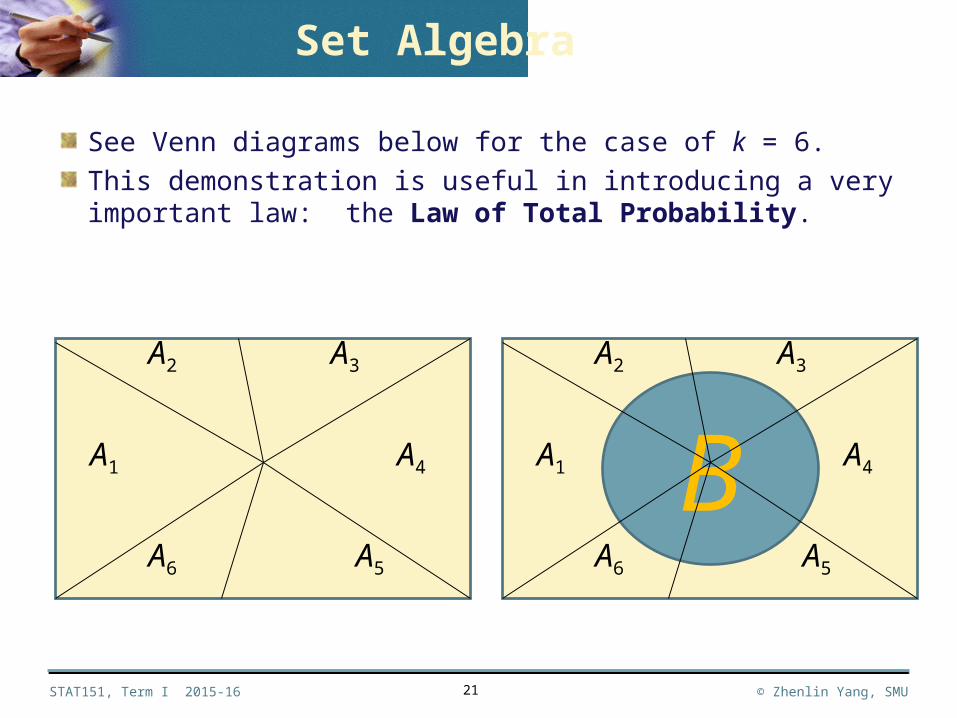
See Venn diagrams below for the case of k = 6.

This demonstration is useful in introducing a very important law: the Law of Total Probability.

A3

A1

A2

A4

A5A6

B

Set Algebra

A3

A1

A2

A4

A5A6


Chapter 1

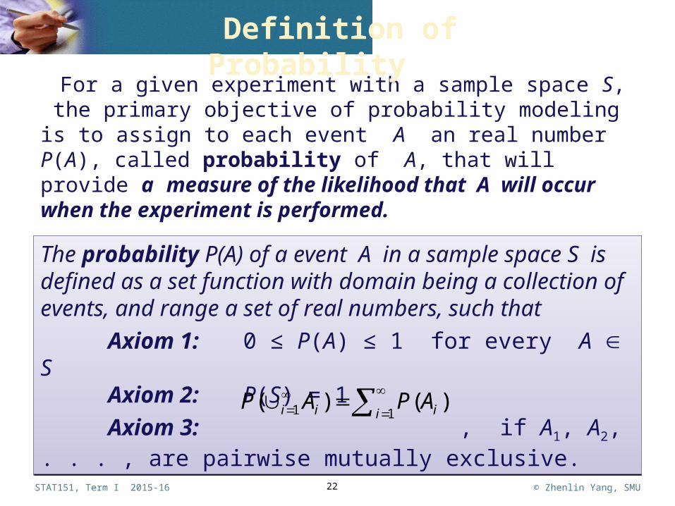
For a given experiment with a sample space S, the primary objective of probability modeling is to assign to each event A an real number P(A), called probability of A, that will provide a measure of the likelihood that A will occur when the experiment is performed.

22

The probability P(A) of a event A in a sample space S is defined as a set function with domain being a collection of events, and range a set of real numbers, such that

Axiom 1: 0 ≤ P(A) ≤ 1 for every A S Axiom 2: P(S) = 1

Axiom 3: , if A1, A2, . . . , are pairwise mutually exclusive.

The probability P(A) of a event A in a sample space S is defined as a set function with domain being a collection of events, and range a set of real numbers, such that

Axiom 1: 0 ≤ P(A) ≤ 1 for every A S Axiom 2: P(S) = 1

Axiom 3: , if A1, A2, . . . , are pairwise mutually exclusive.

Definition of Probability

11 )()(i iii APAP


Chapter 1

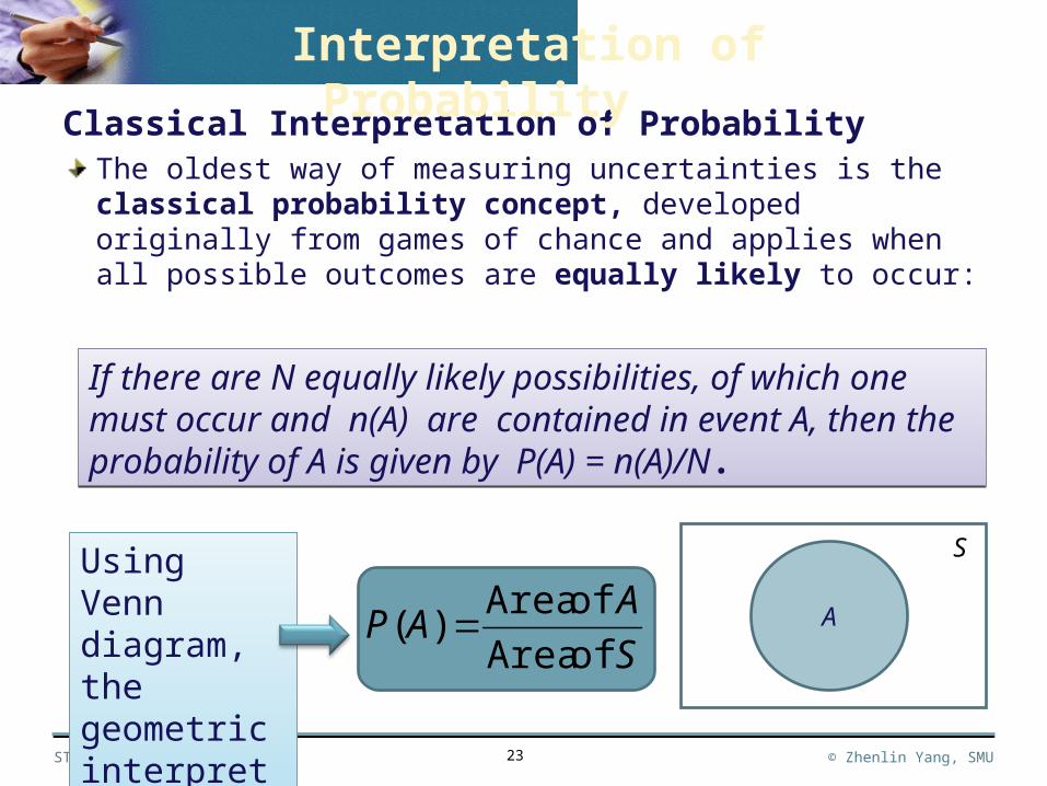
If there are N equally likely possibilities, of which one must occur and n(A) are contained in event A, then the probability of A is given by P(A) = n(A)/N.

If there are N equally likely possibilities, of which one must occur and n(A) are contained in event A, then the probability of A is given by P(A) = n(A)/N.

Classical Interpretation of ProbabilityThe oldest way of measuring uncertainties is the classical probability concept, developed originally from games of chance and applies when all possible outcomes are equally likely to occur:

23

Using Venn diagram, the geometric interpretation:

Using Venn diagram, the geometric interpretation:

S

AAP

of Area

of Area)( A

S

Interpretation of Probability


Chapter 1

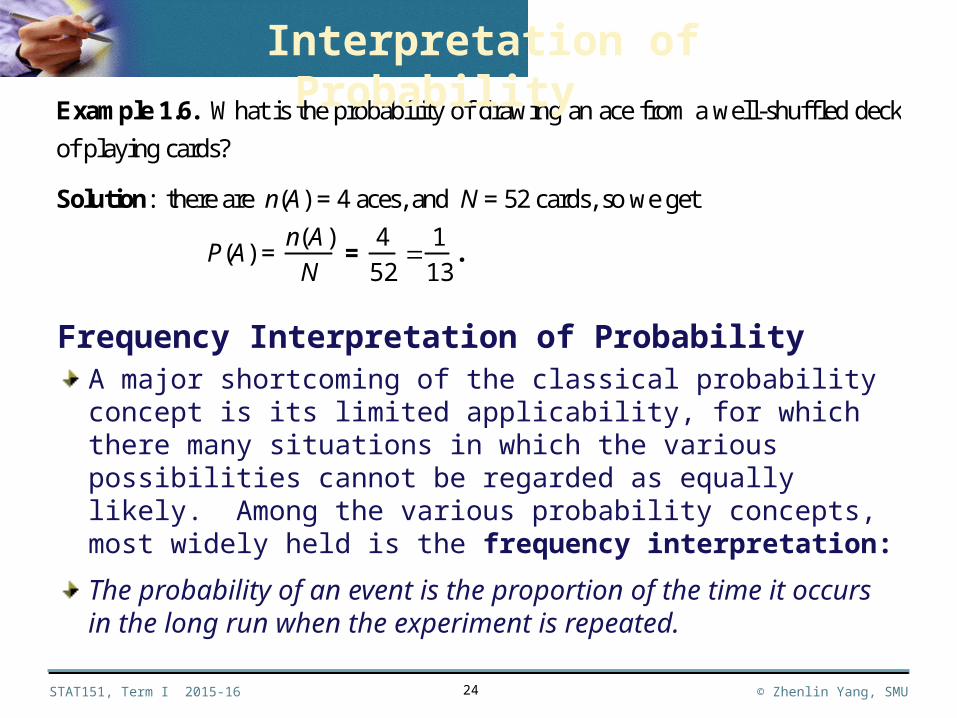
Frequency Interpretation of ProbabilityA major shortcoming of the classical probability concept is its limited applicability, for which there many situations in which the various possibilities cannot be regarded as equally likely. Among the various probability concepts, most widely held is the frequency interpretation:

The probability of an event is the proportion of the time it occurs in the long run when the experiment is repeated.

24

Example 1.6. What is the probability of drawing an ace from a well-shuffled deck

of playing cards?

Solution: there are n(A) = 4 aces, and N = 52 cards, so we get

P(A) = n(A)

N =

4

52

1

13.



Chapter 1

25


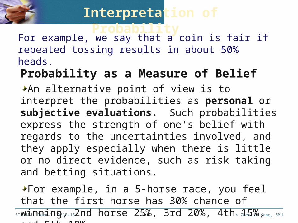
For example, we say that a coin is fair if repeated tossing results in about 50% heads.

Probability as a Measure of BeliefAn alternative point of view is to interpret the probabilities as

personal or subjective evaluations. Such probabilities express the strength of one's belief with regards to the uncertainties involved, and they apply especially when there is little or no direct evidence, such as risk taking and betting situations.

For example, in a 5-horse race, you feel that the first horse has 30% chance of winning, 2nd horse 25%, 3rd 20%, 4th 15%, and 5th 10%.


Chapter 1

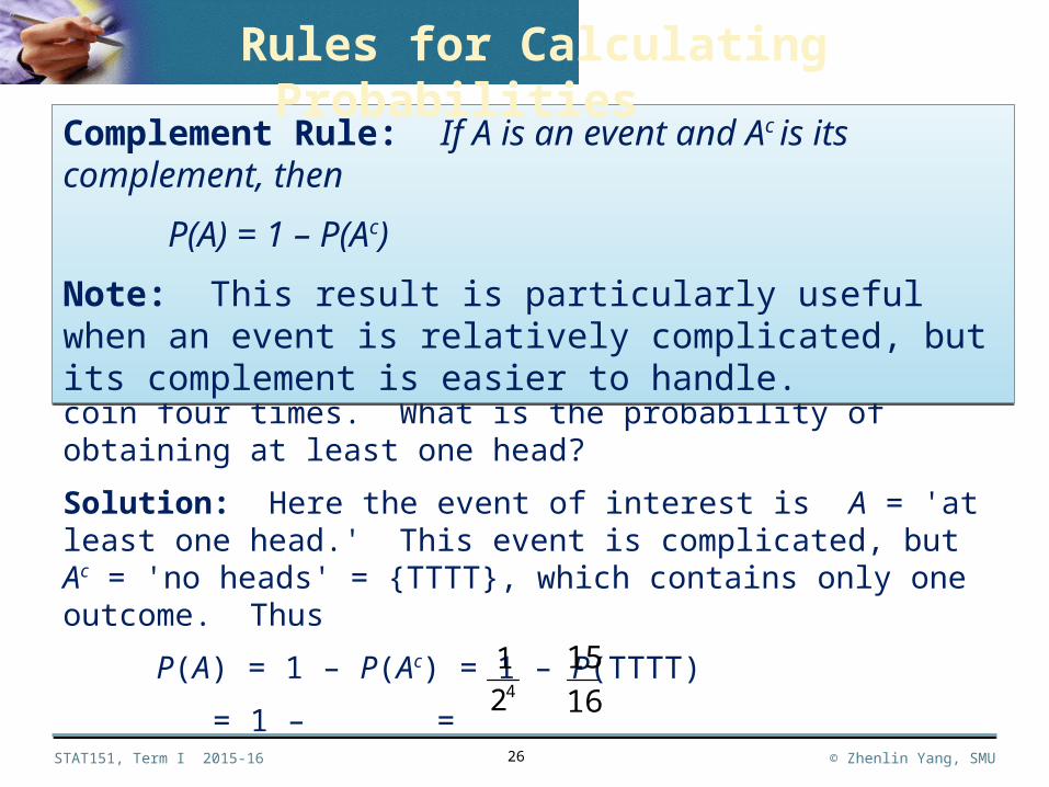
Example 1.7. An experiment consists of tossing a coin four times. What is the probability of obtaining at least one head?

Solution: Here the event of interest is A = 'at least one head.' This event is complicated, but Ac = 'no heads' = {TTTT}, which contains only one outcome. Thus

P(A) = 1 – P(Ac) = 1 – P(TTTT)

= 1 – =

26

42

1

16

15

Complement Rule: If A is an event and Ac is its complement, then

P(A) = 1 – P(Ac)

Note: This result is particularly useful when an event is relatively complicated, but its complement is easier to handle.

Complement Rule: If A is an event and Ac is its complement, then

P(A) = 1 – P(Ac)

Note: This result is particularly useful when an event is relatively complicated, but its complement is easier to handle.



Chapter 1

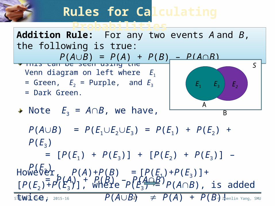
However, P(A)+P(B) = [P(E1)+P(E3)]+ [P(E2)+P(E3)], where P(E3) = P(AB), is added twice, P(AB) P(A) + P(B)!

This can be seen using the Venn diagram on left where E1 = Green, E2 = Purple, and E3 = Dark Green.

27

Addition Rule: For any two events A and B, the following is true:P(AB) = P(A) + P(B) – P(AB)

Addition Rule: For any two events A and B, the following is true:P(AB) = P(A) + P(B) – P(AB)


S

E2E1 E3

A BNote E3 = AB, we have,

P(AB) = P(E1E2E3) = P(E1) + P(E2) + P(E3) = [P(E1) + P(E3)] + [P(E2) + P(E3)] – P(E3) = P(A) + P(B) – P(AB)


Chapter 1

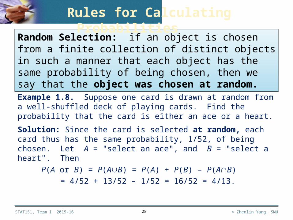
Example 1.8. Suppose one card is drawn at random from a well-shuffled deck of playing cards. Find the probability that the card is either an ace or a heart.

Solution: Since the card is selected at random, each card thus has the same probability, 1/52, of being chosen. Let A = "select an ace", and B = "select a heart". Then

P(A or B) = P(AB) = P(A) + P(B) – P(AB)

= 4/52 + 13/52 – 1/52 = 16/52 = 4/13.

28

Random Selection: if an object is chosen from a finite collection of distinct objects in such a manner that each object has the same probability of being chosen, then we say that the object was chosen at random.

Random Selection: if an object is chosen from a finite collection of distinct objects in such a manner that each object has the same probability of being chosen, then we say that the object was chosen at random.



Chapter 1

29

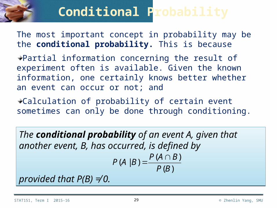
The most important concept in probability may be the conditional probability. This is because

Partial information concerning the result of experiment often is available. Given the known information, one certainly knows better whether an event can occur or not; and

Calculation of probability of certain event sometimes can only be done through conditioning.

The conditional probability of an event A, given that another event, B, has occurred, is defined by

provided that P(B) ≠ 0.

The conditional probability of an event A, given that another event, B, has occurred, is defined by

provided that P(B) ≠ 0.)(

)()|(

BP

BAPBAP



Chapter 1

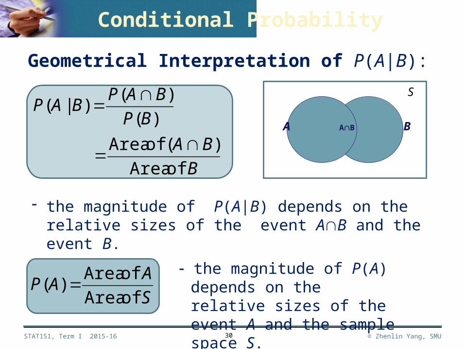
Geometrical Interpretation of P(A|B):

30

S

A AB B

S

AAP

of Area

of Area)(

the magnitude of P(A) depends on the relative sizes of the event A and the sample space S.

B

BA

BP

BAPBAP

of Area

)( of Area

)(

)()|(

the magnitude of P(A|B) depends on the relative sizes of the event AB and the event B.



Chapter 1

31

S

A B

S

A AB B

S

A AB B

S

A B

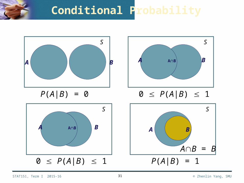
P(A|B) = 0 0 P(A|B) 1

0 P(A|B) 1 P(A|B) = 1

AB = B



Chapter 1

32

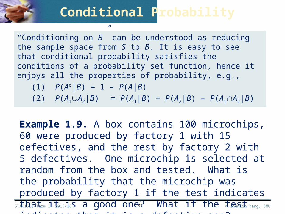
“Conditioning on B” can be understood as reducing the sample space from S to B. It is easy to see that conditional probability satisfies the conditions of a probability set function, hence it enjoys all the properties of probability, e.g.,

(1) P(Ac|B) = 1 – P(A|B)

(2) P(A1A2|B) = P(A1|B) + P(A2|B) – P(A1A2|B)

Example 1.9. A box contains 100 microchips, 60 were produced by factory 1 with 15 defectives, and the rest by factory 2 with 5 defectives. One microchip is selected at random from the box and tested. What is the probability that the microchip was produced by factory 1 if the test indicates that it is a good one? What if the test indicates that it is a defective one?



Chapter 1

33

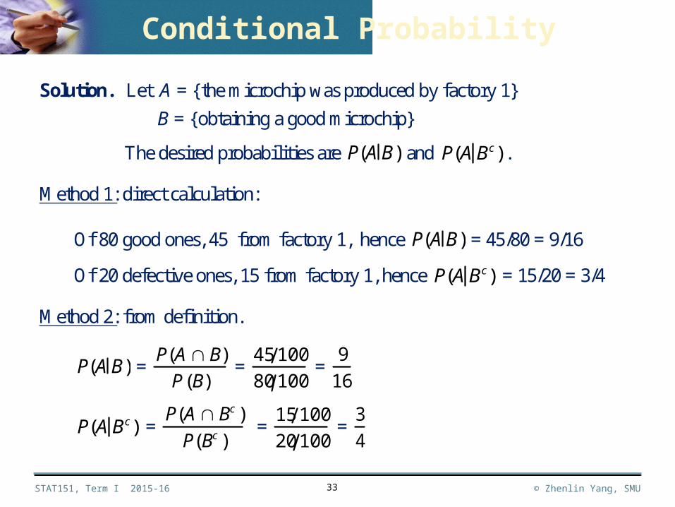
Solution. Let A = {the microchip was produced by factory 1}

B = {obtaining a good microchip}

The desired probabilities are P(A B) and P(A Bc) .

Method 1: direct calculation:

Of 80 good ones, 45 from factory 1, hence P(A B) = 45/80 = 9/16

Of 20 defective ones, 15 from factory 1, hence P(A Bc) = 15/20 = 3/4

Method 2: from definition.

P(A B) = P(A B)

P(B) =

45 100

80 100 =

9

16

P(A Bc) = P(A Bc )

P(Bc ) =

15 100

20 100 =

3

4



Chapter 1

34

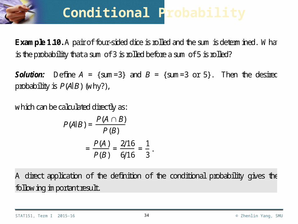
Example 1.10. A pair of four-sided dice is rolled and the sum is determined. What

is the probability that a sum of 3 is rolled before a sum of 5 is rolled?

Solution: Define A = {sum=3} and B = {sum=3 or 5}. Then the desired

probability is P(A B) (why?),

which can be calculated directly as:

P(A B) = P(A B)

P(B)

= P(A)

P(B) =

2 16

6 16 =

1

3.

A direct application of the definition of the conditional probability gives the

following important result.



Chapter 1

35

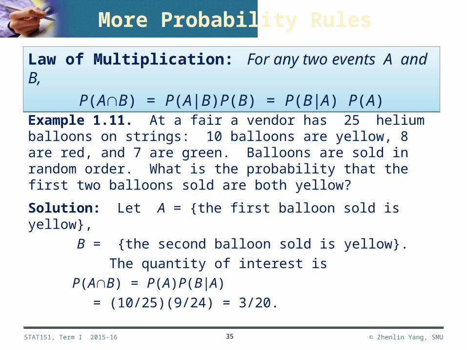
Law of Multiplication: For any two events A and B,

P(AB) = P(A|B)P(B) = P(B|A) P(A)

Law of Multiplication: For any two events A and B,

P(AB) = P(A|B)P(B) = P(B|A) P(A)

Example 1.11. At a fair a vendor has 25 helium balloons on strings: 10 balloons are yellow, 8 are red, and 7 are green. Balloons are sold in random order. What is the probability that the first two balloons sold are both yellow?

Solution: Let A = {the first balloon sold is yellow},

B = {the second balloon sold is yellow}.

The quantity of interest is

P(AB) = P(A)P(B|A)

= (10/25)(9/24) = 3/20.

More Probability Rules


Chapter 1

36

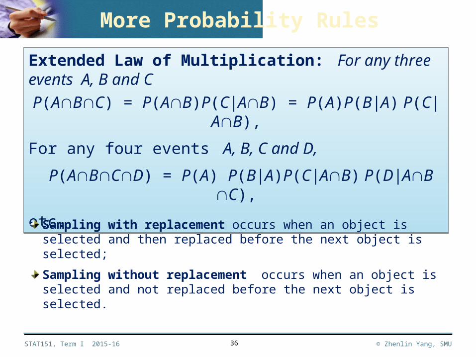
Extended Law of Multiplication: For any three events A, B and C

P(ABC) = P(AB)P(C|AB) = P(A)P(B|A) P(C|AB),

For any four events A, B, C and D,

P(ABCD) = P(A) P(B|A)P(C|AB) P(D|AB C),

etc.

Extended Law of Multiplication: For any three events A, B and C

P(ABC) = P(AB)P(C|AB) = P(A)P(B|A) P(C|AB),

For any four events A, B, C and D,

P(ABCD) = P(A) P(B|A)P(C|AB) P(D|AB C),

etc.

Sampling with replacement occurs when an object is selected and then replaced before the next object is selected;

Sampling without replacement occurs when an object is selected and not replaced before the next object is selected.



Chapter 1

37

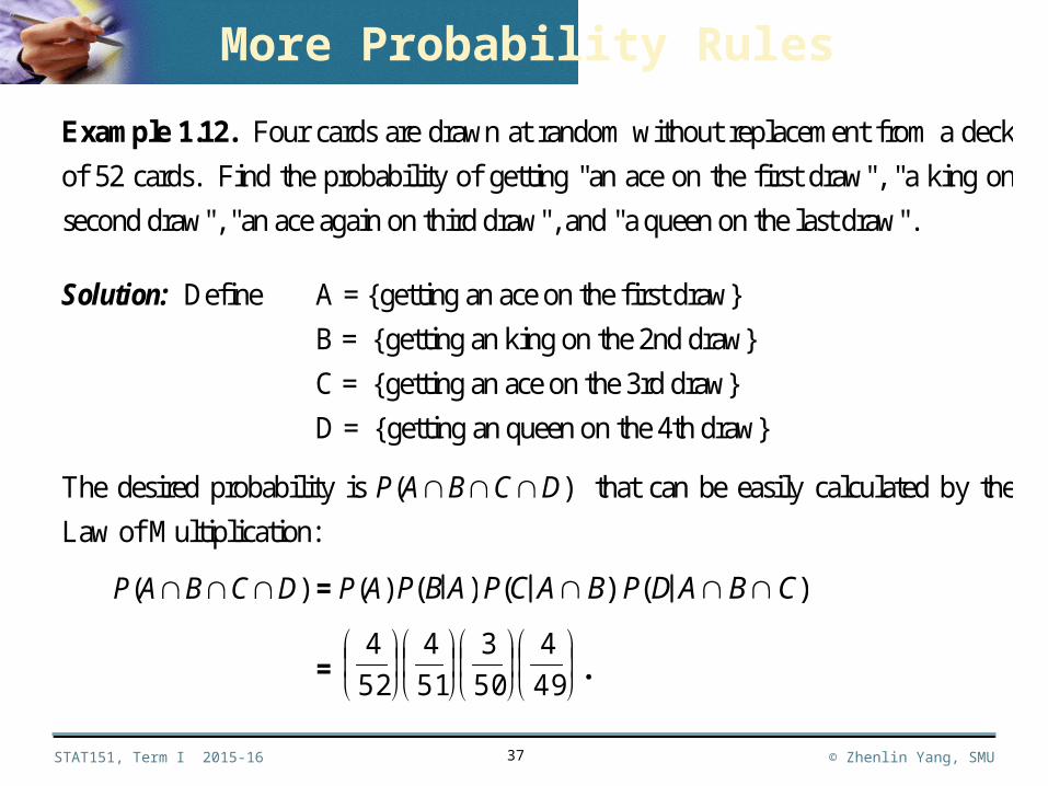
Example 1.12. Four cards are drawn at random without replacement from a deck

of 52 cards. Find the probability of getting "an ace on the first draw", "a king on

second draw", "an ace again on third draw", and "a queen on the last draw".

Solution: Define A = {getting an ace on the first draw}

B = {getting an king on the 2nd draw}

C = {getting an ace on the 3rd draw}

D = {getting an queen on the 4th draw}

The desired probability is P(ABCD) that can be easily calculated by the

Law of Multiplication:

P(ABCD) = P(A) P(B A) P(C A B) P(D ABC)

=

49

4

50

3

51

4

52

4.



Chapter 1

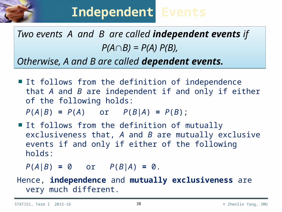
It follows from the definition of independence that A and B are independent if and only if either of the following holds:

P(A|B) = P(A) or P(B|A) = P(B);

It follows from the definition of mutually exclusiveness that, A and B are mutually exclusive events if and only if either of the following holds:

P(A|B) = 0 or P(B|A) = 0.

Hence, independence and mutually exclusiveness are very much different.

38

Two events A and B are called independent events if

P(AB) = P(A) P(B),

Otherwise, A and B are called dependent events.

Two events A and B are called independent events if

P(AB) = P(A) P(B),

Otherwise, A and B are called dependent events.

Independent Events


Chapter 1

39

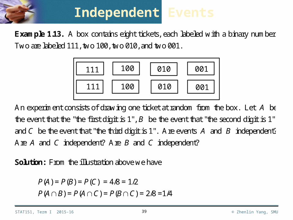
Example 1.13. A box contains eight tickets, each labeled with a binary number.

Two are labeled 111, two 100, two 010, and two 001.

111

111

100

100

010

010

001

001

An experiment consists of drawing one ticket at random from the box. Let A be

the event that the "the first digit is 1", B be the event that "the second digit is 1",

and C be the event that "the third digit is 1". Are events A and B independent?

Are A and C independent? Are B and C independent?

Solution: From the illustration above we have

P(A) = P(B) = P(C) = 4/8 = 1/2

P(AB) = P(AC) = P(BC) = 2/8 =1/4

Independent Events


Chapter 1

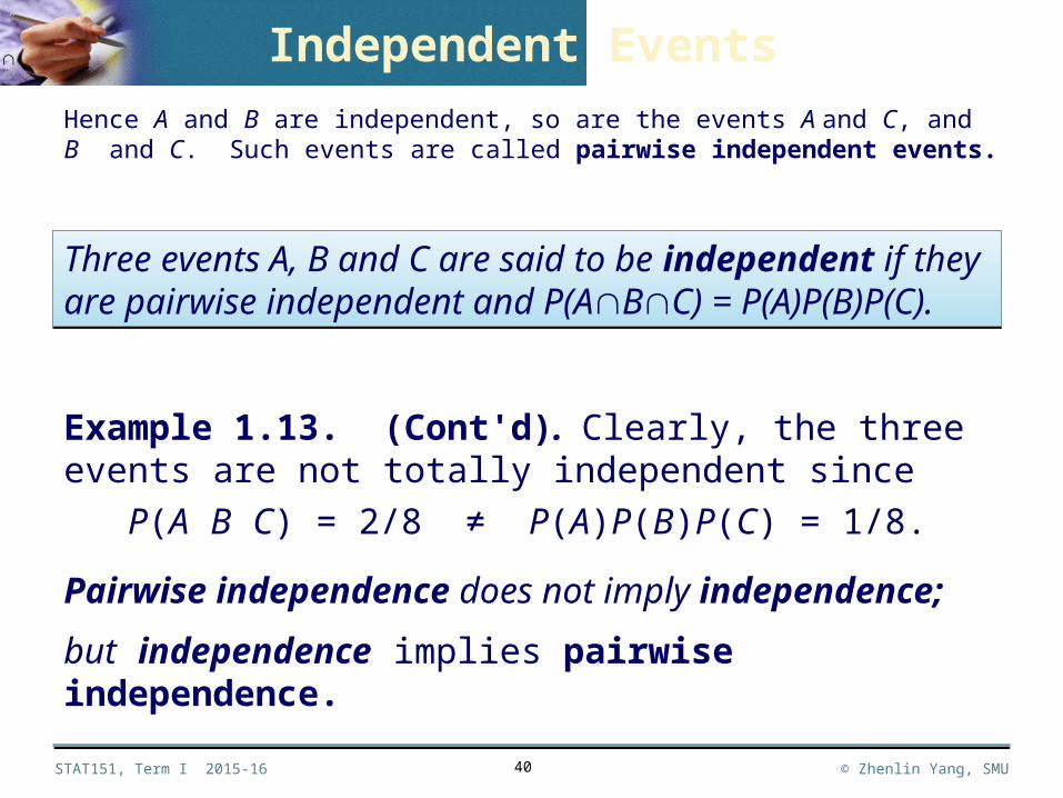
Hence A and B are independent, so are the events A and C, and B and C. Such events are called pairwise independent events.

40

Three events A, B and C are said to be independent if they are pairwise independent and P(ABC) = P(A)P(B)P(C).Three events A, B and C are said to be independent if they are pairwise independent and P(ABC) = P(A)P(B)P(C).

Example 1.13. (Cont'd). Clearly, the three events are not totally independent since

P(A B C) = 2/8 ≠ P(A)P(B)P(C) = 1/8.

Pairwise independence does not imply independence;

but independence implies pairwise independence.

Independent Events


Chapter 1

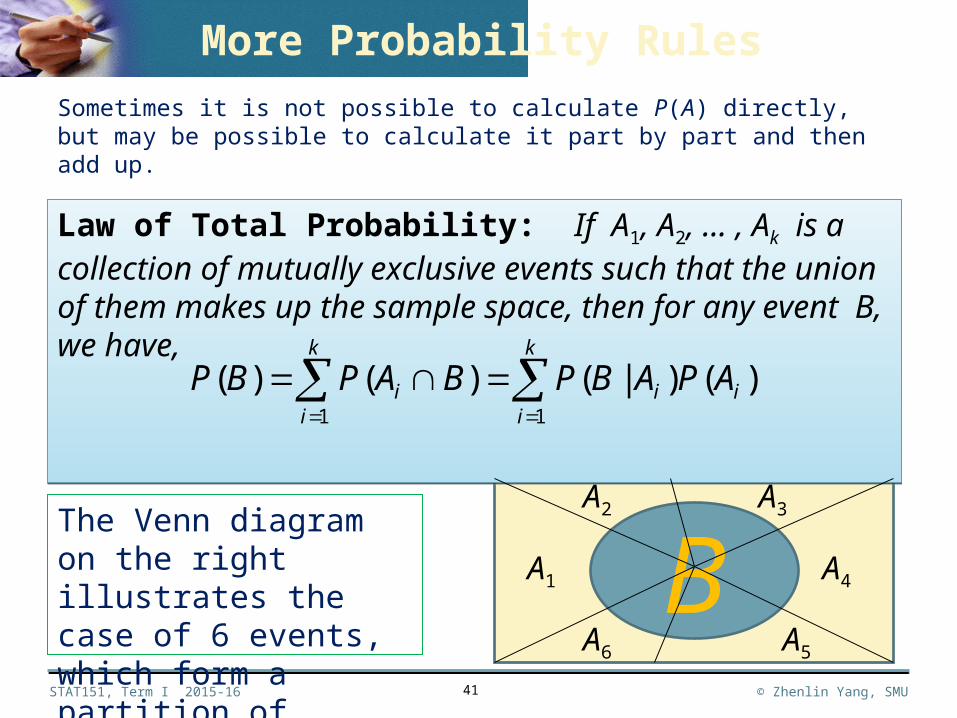
Sometimes it is not possible to calculate P(A) directly, but may be possible to calculate it part by part and then add up.

41

Law of Total Probability: If A1, A2, … , Ak is a collection of mutually exclusive events such that the union of them makes up the sample space, then for any event B, we have,

Law of Total Probability: If A1, A2, … , Ak is a collection of mutually exclusive events such that the union of them makes up the sample space, then for any event B, we have,

k

iii

k

ii APABPBAPBP

11

)()|()()(

BA3

A1

A2

A4

A5A6

The Venn diagram on the right illustrates the case of 6 events, which form a partition of sample space.



Chapter 1

42

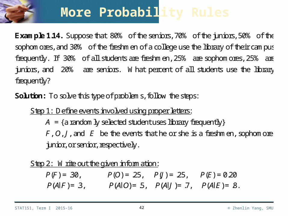
Example 1.14. Suppose that 80% of the seniors, 70% of the juniors, 50% of the

sophomores, and 30% of the freshmen of a college use the library of their campus

frequently. If 30% of all students are freshmen, 25% are sophomores, 25% are

juniors, and 20% are seniors. What percent of all students use the library

frequently?

Solution: To solve this type of problems, follow the steps:

Step 1: Define events involved using proper letters:

A = {a randomly selected student uses library frequently}

F, O, J, and E be the events that he or she is a freshmen, sophomore,

junior, or senior, respectively.

Step 2: Write out the given information:

P(F) = .30, P(O) = .25, P(J) = .25, P(E) = 0.20

P(A F) = .3, P(A O) = .5, P(A J )= .7, P(A E) = .8.



Chapter 1

43

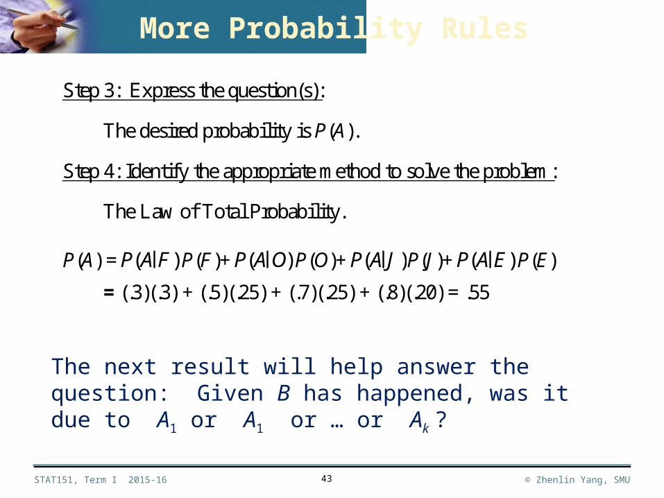
Step 3: Express the question(s):

The desired probability is P(A).

Step 4: Identify the appropriate method to solve the problem:

The Law of Total Probability.

P(A) = P(A F) P(F)+ P(A O) P(O)+ P(A J )P(J)+ P(A E) P(E)

= (.3)(.3) + (.5)(.25) + (.7)(.25) + (.8)(.20) = .55

The next result will help answer the question: Given B has happened, was it due to A1 or A1 or … or Ak ?



Chapter 1

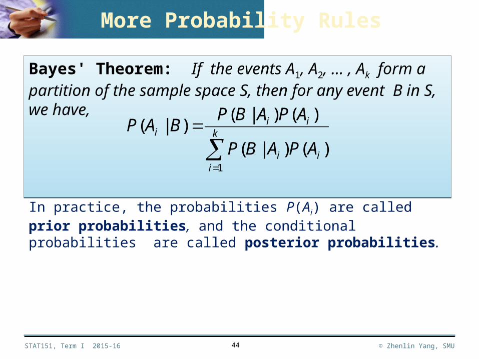
In practice, the probabilities P(Ai) are called prior probabilities, and the conditional probabilities are called posterior probabilities.

44

Bayes' Theorem: If the events A1, A2, … , Ak form a partition of the sample space S, then for any event B in S, we have,

Bayes' Theorem: If the events A1, A2, … , Ak form a partition of the sample space S, then for any event B in S, we have,

k

iii

iii

APABP

APABPBAP

1

)()|(

)()|()|(



Chapter 1

45

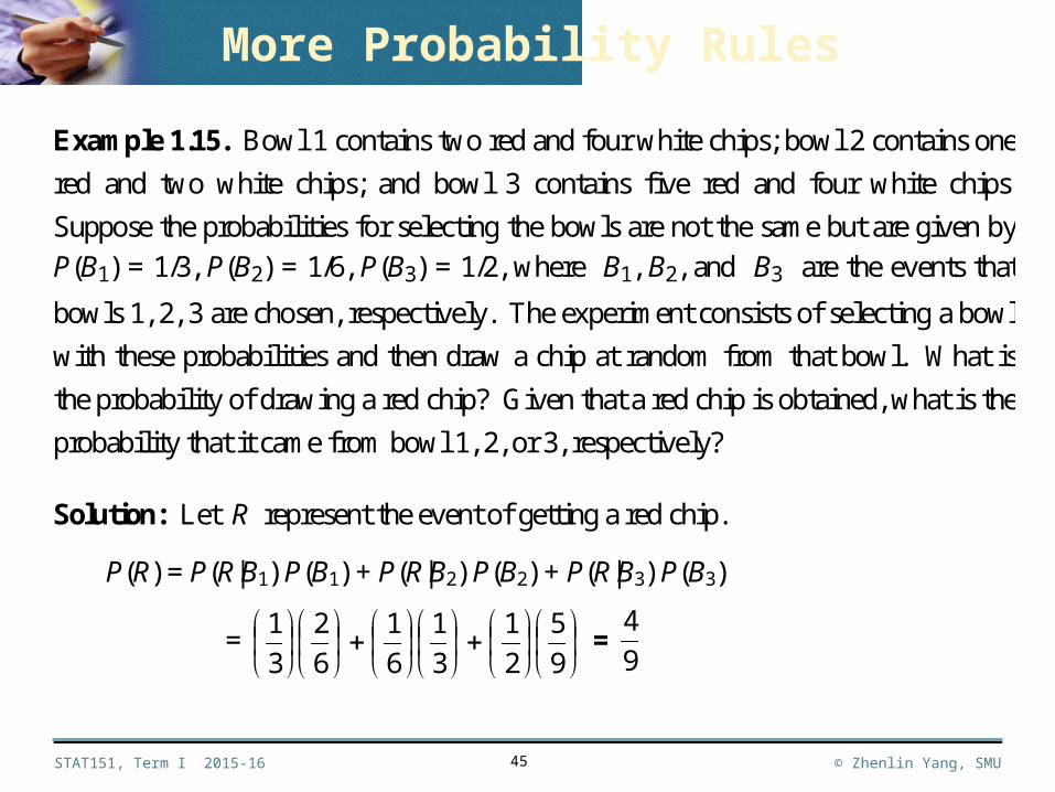
Example 1.15. Bowl 1 contains two red and four white chips; bowl 2 contains one

red and two white chips; and bowl 3 contains five red and four white chips.

Suppose the probabilities for selecting the bowls are not the same but are given by

P(B1) = 1/3, P(B2) = 1/6, P(B3) = 1/2, where B1, B2, and B3 are the events that

bowls 1, 2, 3 are chosen, respectively. The experiment consists of selecting a bowl

with these probabilities and then draw a chip at random from that bowl. What is

the probability of drawing a red chip? Given that a red chip is obtained, what is the

probability that it came from bowl 1, 2, or 3, respectively?

Solution: Let R represent the event of getting a red chip.

P(R) = P(R|B1) P(B1) + P(R|B2) P(B2) + P(R|B3) P(B3)

=

9

5

2

1

3

1

6

1

6

2

3

1 =

9

4



Chapter 1

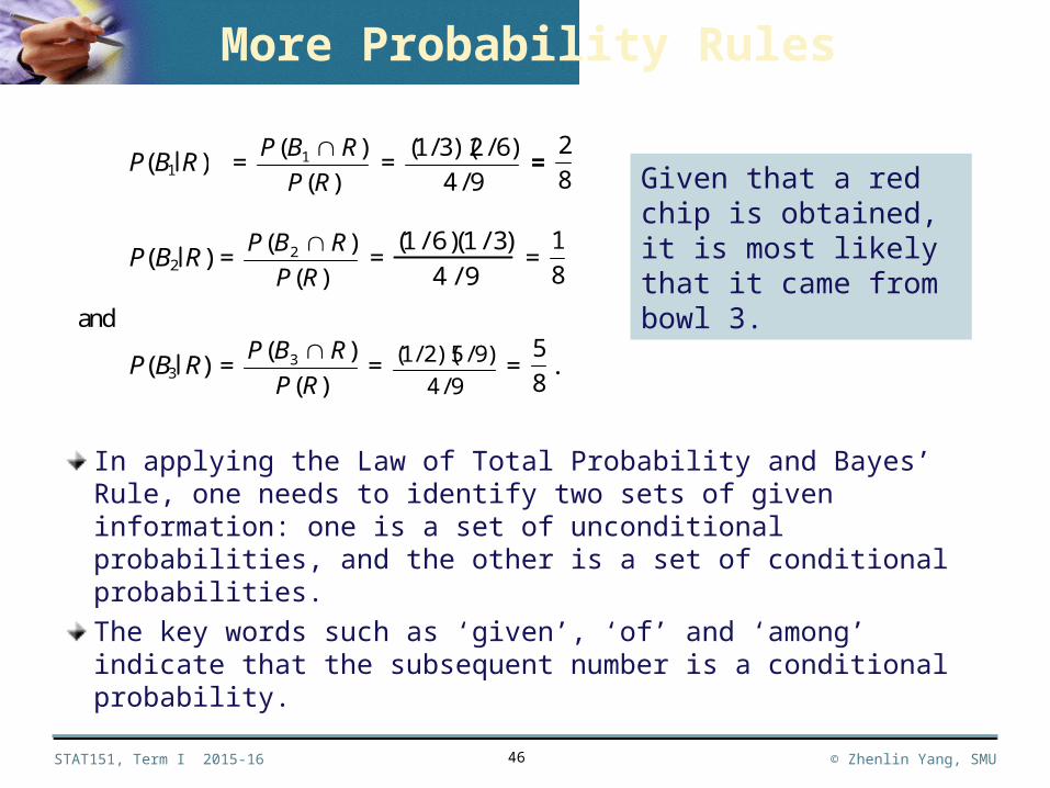
In applying the Law of Total Probability and Bayes’ Rule, one needs to identify two sets of given information: one is a set of unconditional probabilities, and the other is a set of conditional probabilities.

The key words such as ‘given’, ‘of’ and ‘among’ indicate that the subsequent number is a conditional probability.

46

P(B1 R) = )(

)( 1

RP

RBP =

9/4

)6/2)(3/1( =

8

2

P(B2 R) = )(

)( 2

RP

RBP =

(1 / 6)(1 / 3)

4 / 9 =

8

1

and

P(B3 R) = )(

)( 3

RP

RBP =

9/4

)9/5)(2/1( = 8

5.


Given that a red chip is obtained, it is most likely that it came from bowl 3.


Chapter 1

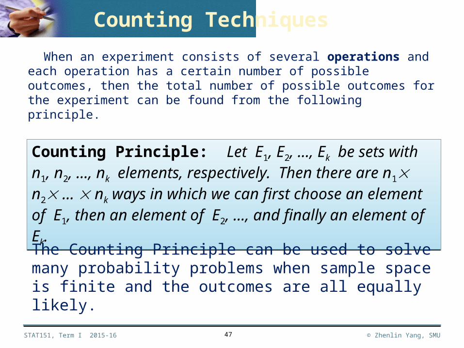
When an experiment consists of several operations and each operation has a certain number of possible outcomes, then the total number of possible outcomes for the experiment can be found from the following principle.

47

Counting Principle: Let E1, E2, ..., Ek be sets with n1, n2, ..., nk elements, respectively. Then there are n1 n2 … nk ways in which we can first choose an element of E1, then an element of E2, ..., and finally an element of Ek.

Counting Principle: Let E1, E2, ..., Ek be sets with n1, n2, ..., nk elements, respectively. Then there are n1 n2 … nk ways in which we can first choose an element of E1, then an element of E2, ..., and finally an element of Ek.

The Counting Principle can be used to solve many probability problems when sample space is finite and the outcomes are all equally likely.

Counting Techniques


Chapter 1

Example 1.16. Suppose that there n routes from a town, A, to another town, B, m routes from town B to a third town, C, and l routes from town C to a fourth town, D. If we decided to go from A to D via B and C. How many different routes are there from A to D?

Solution: In this situation, there are k = 3 operations: A to B, B to C, and C to D, with number of elements (different routes) n, m, and l, respectively. Hence the total number of different routes is n m l.

The above can be argued in a direct way. For each route that we choose from A to B, we have m choices from B to C. Therefore, altogether we have nm choices to go from A to C via B. Furthermore, for each choice from A to C, there are l choices from C to D. Hence we totally have nml choices from A to D.

48

Counting Techniques


Chapter 1

49

Example 1.17. (Birthday Problem) What is the probability that at least two

students of a class of size n have the same birthday? Assume that the birth rates are

constant and there are 365 days a year. Compute the numerical values of such

probabilities for n = 23, 30, 50, and 60.

Solution: There are 365 possibilities for the birthdays of each of the n students.

Therefore, there are 365n possible combinations of the birthdays of n students. Let

A = {no two students have the same birthday}, then

P(A) = n

n

365

)]1(365[364365

The desired probability is thus, P(Ac) = 1– P(A).

Now, n = 23, P(Ac) = 0.507; n = 30, P(Ac) = 0.706; n = 50, P(Ac) = 0.970; n = 60,

P(Ac) = 0.995.

Counting Techniques


Chapter 1

For example, if A = {a, b, c, d}, then ab and ba are two-element permutations of A; bcd, bdc, cbd, cdb, dbc and dcb are the three-element permutation of A.

50

Permutation: An ordered arrangement of r objects from a set A containing n objects (0 ≤ r ≤ n) is called an r–element permutation of A or a permutation of the elements of A taken r at a time.

Permutation: An ordered arrangement of r objects from a set A containing n objects (0 ≤ r ≤ n) is called an r–element permutation of A or a permutation of the elements of A taken r at a time.

Permutation Rule: Let nPr denote the total number of permutations of a set A containing n elements taken r at a time. Then

nPr = n(n – 1)(n – 2) ... (n –r + 1) =

Permutation Rule: Let nPr denote the total number of permutations of a set A containing n elements taken r at a time. Then

nPr = n(n – 1)(n – 2) ... (n –r + 1) = )!(

!

rn

n

Counting Techniques


Chapter 1

Example 1.18. In how many different ways can a president, a treasure, and a secretary be selected from a group of 20 people to form a committee?

Solution: nPr = 20P3 = 201918 = 6840.

–––There are 20 ways to choose a president, 19 ways of choosing a treasure after a president has been chosen, and 18 choices left for a secretary.

51

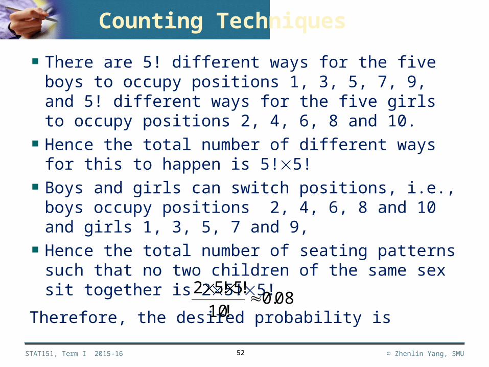
Example 1.19. If five boys and five girls sit in a row in a random order, what is the probability that no two children of the same sex sit together?

Solution: First we know that there are 10! possible seating patterns in total for the 10 children. In order that no two children of the same sex sit together, boys must occupy positions 1, 3, 5, 7 and 9 and girls 2, 4, 6, 8 and 10.

Counting Techniques


Chapter 1

There are 5! different ways for the five boys to occupy positions 1, 3, 5, 7, 9, and 5! different ways for the five girls to occupy positions 2, 4, 6, 8 and 10.

Hence the total number of different ways for this to happen is 5!5!

Boys and girls can switch positions, i.e., boys occupy positions 2, 4, 6, 8 and 10 and girls 1, 3, 5, 7 and 9,

Hence the total number of seating patterns such that no two children of the same sex sit together is 25!5!

Therefore, the desired probability is

52

08.0!10

!5!52

Counting Techniques


Chapter 1

53

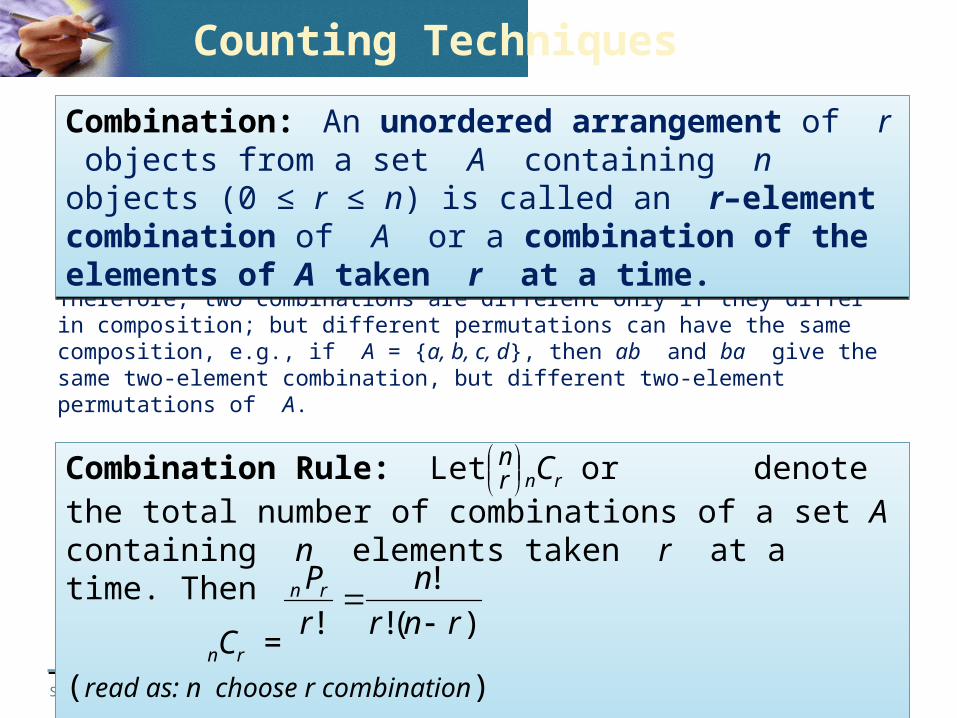
Therefore, two combinations are different only if they differ in composition; but different permutations can have the same composition, e.g., if A = {a, b, c, d}, then ab and ba give the same two-element combination, but different two-element permutations of A.

Combination: An unordered arrangement of r objects from a set A containing n objects (0 ≤ r ≤ n) is called an r–element combination of A or a combination of the elements of A taken r at a time.

Combination: An unordered arrangement of r objects from a set A containing n objects (0 ≤ r ≤ n) is called an r–element combination of A or a combination of the elements of A taken r at a time.

Combination Rule: Let nCr or denote the total number of combinations of a set A containing n elements taken r at a time. Then

nCr = (read as: n choose r combination)

Combination Rule: Let nCr or denote the total number of combinations of a set A containing n elements taken r at a time. Then

nCr = (read as: n choose r combination)

rn

)!(!

!

! rnr

n

r

Prn

Counting Techniques


Chapter 1

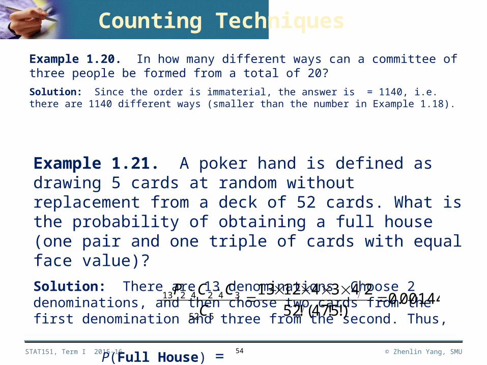
Example 1.20. In how many different ways can a committee of three people be formed from a total of 20?

Solution: Since the order is immaterial, the answer is = 1140, i.e. there are 1140 different ways (smaller than the number in Example 1.18).

54

Counting Techniques

Example 1.21. A poker hand is defined as drawing 5 cards at random without replacement from a deck of 52 cards. What is the probability of obtaining a full house (one pair and one triple of cards with equal face value)?

Solution: There are 13 denominations. Choose 2 denominations, and then choose two cards from the first denomination and three from the second. Thus,

P(Full House) = 00144.0)!5!47(!52

24341213

552

3424213

C

CCP


Chapter 1

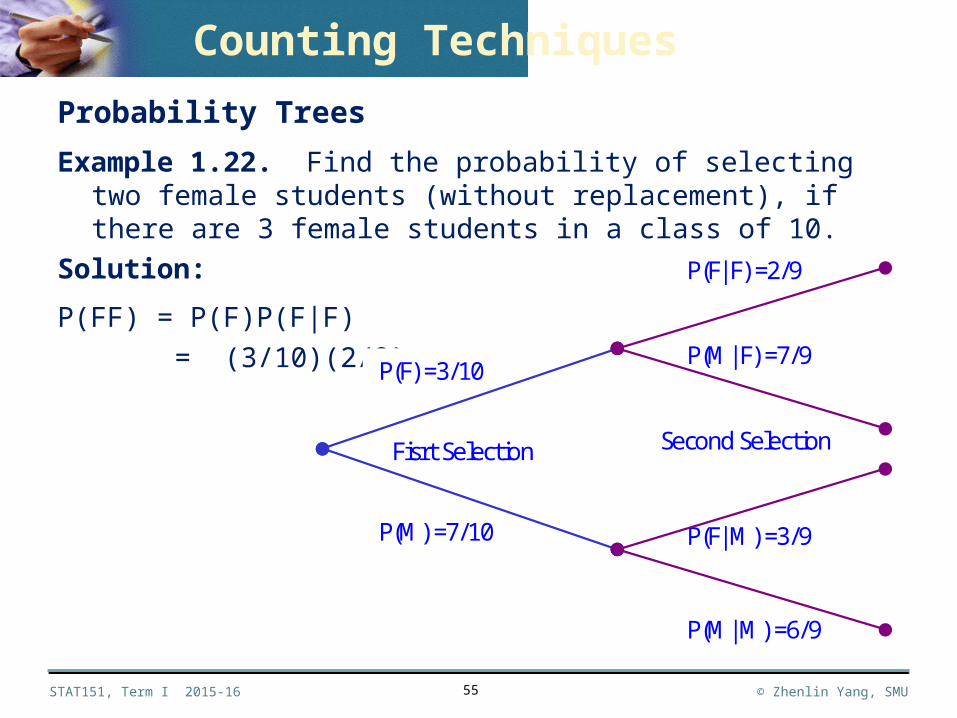
Probability Trees

Example 1.22. Find the probability of selecting two female students (without replacement), if there are 3 female students in a class of 10.

Solution:

P(FF) = P(F)P(F|F)

= (3/10)(2/9)

55

P(F|F) =2/9

Second Selection Fisrt Selection

P(M|M) =6/9

P(F|M) =3/9

P(F) =3/10

P(M) =7/10

P(M|F) =7/9

Counting Techniques

Documents

[email protected] STAT151: Introduction to Statistical Theory Term I, 2015-2016 Yang Zhenlin