1
A Multi-Resolution Terrain Model for Efficient
Visualization Query Processing
Kai Xu, Xiaofang Zhou,Member, IEEE,Xuemin Lin, Heng Tao Shen, and Ke Deng
Abstract
Multi-resolution Triangular Mesh (MTM) models are widely used to improve the performance of large terrain
visualization by replacing the original model with simplified one. MTM models, which consist of both original and
simplified data, are commonly stored in spatial database systems due to their size. The relatively slow access speed
of disk makes data retrieval the bottle-neck of such terrain visualization systems. Existing spatial access methods
proposed to address this problem rely on main-memory MTM models, which leads to significant overhead during
query processing. In this paper, we approach the problem from a new perspective and propose a novel MTM called
Direct Meshes that is designed specifically for secondary storage. It supports available indexing methods natively
and requires no modification to MTM structure. Experiment results, which are based on two real-world datasets,
show an average of 5-10 times performance improvement over the existing methods.
Index Terms
Multi-resolution visualization, spatial database systems
I. I NTRODUCTION
T Errain visualization plays an essential role in a wide range of applications such as gaming [1],
[2], virtual reality [3], [4], 3D environmental analysis [5], [6], and many GIS applications [7], [8].
Terrain data obtained from the natural environment is usually very large. For instance, the US Geology
Survey (www.usgs.gov) provides digital elevation data covering most parts of the US, sampled at 10-
or 30-meter resolution. The volume of entire dataset is measured in terabytes. The visualization of such
2
datasets usually requires excessive resources and the resolution can be unnecessarily high in many cases.
A typical scenario is that when a terrain with millions of polygons is displayed on a device with limited
resolution, it appears to be overly dense and illegible. Fig. 1(a) shows an example with a relatively small
number of triangles (10,000), but the top-right part of the terrain already appears to be unnecessarily
dense.Multi-resolutiontechniques are introduced to address this problem by replacing the original terrain
(a) 10,000 triangles (b) 10,000 triangles with texture (c) 1,000 triangles (d) 1,000 triangles with texture
Fig. 1. Terrain at multiple resolutions
model with a simplified approximation (mesh) constructed according to application requirements [9]. It
reduces the resource requirements significantly while introducing an acceptable sacrifice of visual quality.
Following the previous example, a simplified mesh is shown in Fig. 1(c) with only 1000 triangles. The
difference is hardly noticeable after texture is applied (Fig. 1(b) and 1(d)).
Mesh construction, which is essentially the simplification of the original model, is expensive due to
the usually large size of the terrain dataset. The possible benefit of using a mesh can be overcome by its
expensive construction. The fact that terrain data can be used at any resolution and one mesh can have
varying resolutions means that it is not feasible to pre-generate meshes at a fixed number of resolutions.
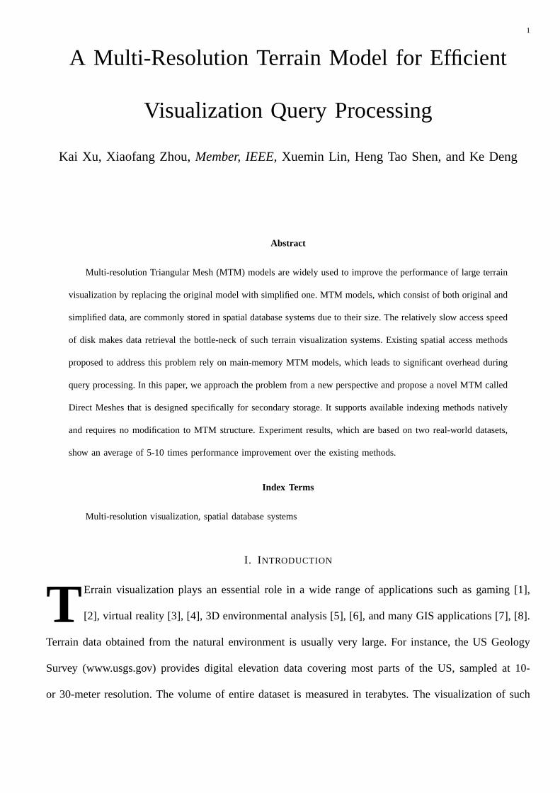
An example that requires mesh with varying resolution is shown in Figure 2; to have a uniform-resolution
mesh on display (Fig. 2(a)), the actual resolution needs to decrease with the distance from the viewpoint
(Fig. 2(b)).
Multi-resolution Triangular Mesh (MTM)models are proposed to address this problem. Most MTM
models adopt a tree-like data structure, and each node stores an approximation of the union of its child
nodes’ data. Mesh construction starts from the root, which contains the least detailed data, and this coarse
3
(a) Display (b) Mesh
Fig. 2. Mesh with variable resolution
mesh is refined progressively by recursively replacing part of it with the more detailed data stored at child
nodes until the desired resolution is achieved (the details are provided in Section II). Since it starts with
a very simple mesh rather that the original model, this procedure can significantly reduce construction
costs. The initial coarse mesh can be refined to any resolution available and every part can be refined to
a different level of detail, which results in a mesh with varying resolution.
MTMs are usually very large because they include both the original model and simplified data. This
makes spatial database systems a common choice for their storage. Since the disk access speed is several-
order slower than that of main memory, data retrieval becomes the bottle-neck for terrain visualization
systems relying on spatial database systems [10], [11]. This problem has attracted significant research
attention from both the computer graphics and database research communities. While the graphics com-
munity mainly focuses on designing new MTMs suitable for secondary storage [12], [13], [14], database
researchers have been proposing spatial access methods to improve data retrieval efficiency [15], [16], [17],
[10], [11]. The former approach usually requires the rebuilding of MTM, which is very time consuming;
the latter can avoid this problem, but they rely on the tree-like MTM structure, which commonly leads to
significant retrieval overhead during query processing. In this paper, we follow the spatial-access-method
approach but address the problem from a new perspective. We propose a new MTM calledDirect Meshes.
Different from both existing approaches, the Direct Meshes is a secondary-storage MTM that requires
no change to the original MTM structure (no rebuilding) and is designed to seamlessly integrate with

4
well-studied spatial access methods (such as the R∗-tree [18] used in this paper). An average improvement
of 5-10 times is observed from the evaluation results when comparing against the best existing methods.
A shorter version of this work appeared in [19]. The previous work is extended from several aspects.
First, formal definitions of the problem and relevant concepts are included; a general multi-resolution
visualization query is introduced to unify the two types of queries in the previous work. Secondly, the
Direct Meshes construction algorithm is presented, together with its correctness proof and running time
/ storage requirement analysis; the design issues such as the topology encoding scheme and the choice
of spatial access method are discussed in detail. Thirdly, the query processing algorithm based on the
new multi-resolution visualization query replaces the old one; its cost analysis and comparison against
existing methods are also added. Fourth, the core of the Direct Meshes, the topology encoding scheme,
is enhanced to eliminate the inefficient data retrieval discovered in the previous performance study. Last
but not least, extensive test results, including the comparison between the Direct Meshes with different
encoding schemes, are added to make the performance evaluation more comprehensive.
The remainder of this paper is organized as follows. The problem is defined in Section II after the
introduction to MTM visualization. Related work is reviewed in Section III. The topological information
required for multi-resolution visualization and its encoding scheme in Direct Meshes are discussed in
Section IV. The Direct Meshes is introduced in Section V, together with its construction algorithm,
correctness proof, and complexity analysis. Section VI discusses the query processing using the Direct
Meshes, which includes the choice of spatial access methods, cost analysis, and two optimization tech-
niques. A performance study using two sets of real-life terrain data is reported in Section VII. Finally,
the paper is concluded in Section VIII.
II. M ULTI -RESOLUTION V ISUALIZATION
In this section, we start with an overview of multi-resolution visualization, followed by the definition
of selective refinement query, which is the main focus of this paper. After that,Progressive meshes— one
of the most popular MTMs — is used as an example to illustrate selective refinement query processing.
5
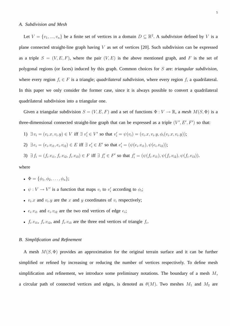
A. Subdivision and Mesh
Let V = {v1, ..., vn} be a finite set of vertices in a domainD ⊆ R2. A subdivisiondefined byV is a
plane connected straight-line graph havingV as set of vertices [20]. Such subdivision can be expressed
as a tripleS = (V,E, F ), where the pair(V,E) is the above mentioned graph, andF is the set of
polygonal regions (or faces) induced by this graph. Common choices forS are: triangular subdivision,
where every regionfi ∈ F is a triangle;quadrilateral subdivision, where every regionfi a quadrilateral.
In this paper we only consider the former case, since it is always possible to convert a quadrilateral
quadrilateral subdivision into a triangular one.
Given a triangular subdivisionS = (V, E, F ) and a set of functionsΦ : V → R, a meshM(S, Φ) is a
three-dimensional connected straight-line graph that can be expressed as a triple(V ′, E ′, F ′) so that:
1) ∃ vi = (vi.x, vi.y) ∈ V iff ∃ v′i ∈ V ′ so thatv′i = ψ(vi) = (vi.x, vi.y, φi(vi.x, vi.y));
2) ∃ ei = (ei.vi1, ei.vi2) ∈ E iff ∃ e′i ∈ E ′ so thate′i = (ψ(ei.vi1), ψ(ei.vi2));
3) ∃ fi = (fi.vi1, fi.vi2, fi.vi3) ∈ F iff ∃ f ′i ∈ F ′ so thatf ′i = (ψ(fi.vi1), ψ(fi.vi2), ψ(fi.vi3)).
where
• Φ = {φ1, φ2, . . . , φn};
• ψ : V → V ′ is a function that mapsvi to v′i according toφi;
• vi.x andvi.y are thex andy coordinates ofvi respectively;
• ei.vi1 andei.vi2 are the two end vertices of edgeei;
• fi.vi1, fi.vi2, andfi.vi3 are the three end vertices of trianglefi.
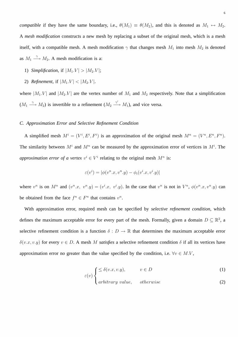
B. Simplification and Refinement
A mesh M(S, Φ) provides an approximation for the original terrain surface and it can be further
simplified or refined by increasing or reducing the number of vertices respectively. To define mesh
simplification and refinement, we introduce some preliminary notations. The boundary of a meshM ,
a circular path of connected vertices and edges, is denoted asθ(M). Two meshesM1 and M2 are
6
compatibleif they have the same boundary, i.e.,θ(M1) ≡ θ(M2), and this is denoted asM1 ↔ M2.
A mesh modificationconstructs a new mesh by replacing a subset of the original mesh, which is a mesh
itself, with a compatible mesh. A mesh modificationγ that changes meshM1 into meshM2 is denoted
asM1γ−→ M2. A mesh modification is a:
1) Simplification, if |M1.V | > |M2.V |;
2) Refinement, if |M1.V | < |M2.V |.
where |M1.V | and |M2.V | are the vertex number ofM1 andM2 respectively. Note that a simplification
(M1γ−→ M2) is invertible to a refinement (M2
γ′−→ M1), and vice versa.
C. Approximation Error and Selective Refinement Condition
A simplified meshM i = (V i, Ei, F i) is an approximation of the original meshMn = (V n, En, F n).
The similarity betweenM i andMn can be measured by the approximation error of vertices inM i. The
approximation error of a vertexvi ∈ V i relating to the original meshMn is:
ε(vi) = |φ(vn.x, vn.y)− φi(vi.x, vi.y)|
wherevn is on Mn and (vn.x, vn.y) = (vi.x, vi.y). In the case thatvn is not in V n, φ(vn.x, vn.y) can
be obtained from the facefn ∈ F n that containsvn.
With approximation error, required mesh can be specified byselective refinement condition, which
defines the maximum acceptable error for every part of the mesh. Formally, given a domainD ⊆ R2, a
selective refinement condition is a functionδ : D → R that determines the maximum acceptable error
δ(v.x, v.y) for everyv ∈ D. A meshM satisfiesa selective refinement conditionδ if all its vertices have
approximation error no greater than the value specified by the condition, i.e.∀v ∈ M.V ,
ε(v)
≤ δ(v.x, v.y), v ∈ D (1)
arbitrary value, otherwise (2)

7
D. Multi-Resolution Triangular Mesh
A multi-resolution triangular mesh (MTM) representation of a meshMn can be built by recursively
applying a sequence of simplifications( αn−1, αn−2, ..., α0) to Mn. Each simplification step produces a
simpler mesh, i.e.,M i−1 (results fromM i αi−1−→ M i−1) has fewer vertices thanM i. The sequence of
meshes
Mn αn−1−→ Mn−1 αn−2−→, · · · , α1−→ M1 α0−→ M0
have a monotonically reducing number of vertices. Due to the large size of the original meshMn and the
fact that mesh simplification is invertible, the common approach stores the simplest mesh together with a
sequence of refinement, i.e.,
M0 β0−→ M1 β1−→, · · · , βn−2−→ Mn−1 βn−1−→ Mn
whereβi is the inverse of theαi, 0 ≤ i ≤ n− 1. If we regard the initial meshM0 as a refinement from
a null mesh, the set of refinementsR = {M0, β0, β1, . . . , βn−1} is the multi-resolution triangular mesh
(MTM) representation of meshMn.
Early MTM models only allow construction of meshes that appear during simplification. This is achieved
by only allowing a refinement sequence that follows the exact reverse order of simplification. Such an
approach guarantees a proper triangulated mesh given it is checked during MTM construction. However,
this total ordering can be quite restrictive for selective refinement query. Later approaches adopt a less
restrictive partial ordering, which can be described as a directed acyclic graph (DAG) whose nodes
represent refinement and edges are the dependency among refinements. An MTM based on such partial
ordering can be defined as a DAGG = (R, ER), whereR = {M0, β0, β1, . . . , βn−1} is the set of mesh
refinements andER is a set of directed edges defined onR × R such that there is a directed edge
(βi, βj), i 6= j if βj refines part of the mesh results fromβi. To avoid confusion, we refer to the point in
a mesh as “vertex” and the point in an MTM as “node” from here on.

8
E. Selective Refinement Query
Selective refinement constructs a mesh according to a given conditionδ. Usually there are multiple
meshes that meet the selective refinement condition because only the upper bound of mesh error is given.
Among them, the one with the least number of vertices is commonly preferred as the result of a selective
refinement. Given an MTMG and selective refinement conditionδ, a selective refinement queryQ(G, δ)
returns a meshM where:
1) M satisfiesδ;
2) |M.V | ≤ |M i.V | for all δ-satisfying meshesM i that can be constructed fromG.
We say meshM is feasiblerelating toδ.
In this paper we focus on selective refinement query processing in multi-resolution terrain databases.
Our goal is to reduce the data retrieval for a selective refinement query. One of the main constraints is to
support selective refinement with varying resolution as described in Section I. Formally, given an MTM
G and a selective refinement conditionδ, we try to minimize the overall I/O costDA(Q(G, δ)), whereδ
is a function of mesh vertex location.
F. Progressive Meshes
For this paper we use theProgressive Meshes[21], one of the most popular MTMs, as an example to
illustrate our work. The Progressive Meshes is built upon a simplification process callededge collapse, in
which one edge collapses into a new vertex (Fig. 3(a)). The new vertex (v9) is recorded as the parent node
of the two end nodes (v1 andv2) of the collapsed edge (Fig. 3(b)). Edge collapse is repeated recursively
on the resulting mesh until only one vertex is left, and the resulting structure is an unbalanced binary tree
(Fig. 3(c)). Progressive Meshes stores the final mesh (one vertex) and a set ofvertex splits(the inverse
of edge collapses, Fig. 3(a)). Progressive Meshes can be defined as a directed binary treeGp = (Np, Ep)
where every noden in Np represents a vertex and every edgee in Ep pointing from the parent to its
children.

9
(a) Edge collapse and vertex split (b) Edge collapse
structure
(c) Tree structure of Progressive
Meshes
Fig. 3. Progressive Meshes
A linear-time incremental algorithm is proposed in [22] for selective refinement query. The algorithm
starts with a mesh with root only and iterates through its vertex list, during which vertex, whose approx-
imation error is greater than the maximum acceptable error, is replaced with its children recursively. The
algorithm stops when the mesh satisfies the selective refinement condition. The pseudo code in Algorithm
1 outlines the majors steps.
Algorithm 1 : Selective Refinement Algorithm for Progressive Meshes
Input : Progressive MeshesGp = (Np, Ep), selective refinement conditionδ
Output : meshM
M ← M0;1
for every vertexv ∈ M.V do2
if ε(v) > δ(v) then3
removev from M.V ;4
appendv1, v2 (the children ofv) to M.V ;5
endif6
endfor7
return M8
10
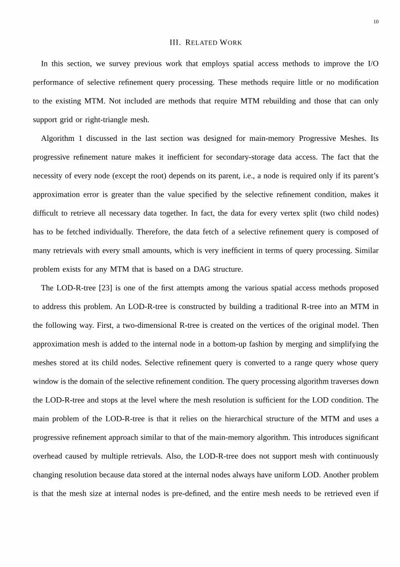
III. R ELATED WORK
In this section, we survey previous work that employs spatial access methods to improve the I/O
performance of selective refinement query processing. These methods require little or no modification
to the existing MTM. Not included are methods that require MTM rebuilding and those that can only
support grid or right-triangle mesh.
Algorithm 1 discussed in the last section was designed for main-memory Progressive Meshes. Its
progressive refinement nature makes it inefficient for secondary-storage data access. The fact that the
necessity of every node (except the root) depends on its parent, i.e., a node is required only if its parent’s
approximation error is greater than the value specified by the selective refinement condition, makes it
difficult to retrieve all necessary data together. In fact, the data for every vertex split (two child nodes)
has to be fetched individually. Therefore, the data fetch of a selective refinement query is composed of
many retrievals with every small amounts, which is very inefficient in terms of query processing. Similar
problem exists for any MTM that is based on a DAG structure.
The LOD-R-tree [23] is one of the first attempts among the various spatial access methods proposed
to address this problem. An LOD-R-tree is constructed by building a traditional R-tree into an MTM in
the following way. First, a two-dimensional R-tree is created on the vertices of the original model. Then
approximation mesh is added to the internal node in a bottom-up fashion by merging and simplifying the
meshes stored at its child nodes. Selective refinement query is converted to a range query whose query
window is the domain of the selective refinement condition. The query processing algorithm traverses down
the LOD-R-tree and stops at the level where the mesh resolution is sufficient for the LOD condition. The
main problem of the LOD-R-tree is that it relies on the hierarchical structure of the MTM and uses a
progressive refinement approach similar to that of the main-memory algorithm. This introduces significant
overhead caused by multiple retrievals. Also, the LOD-R-tree does not support mesh with continuously
changing resolution because data stored at the internal nodes always have uniform LOD. Another problem
is that the mesh size at internal nodes is pre-defined, and the entire mesh needs to be retrieved even if
11
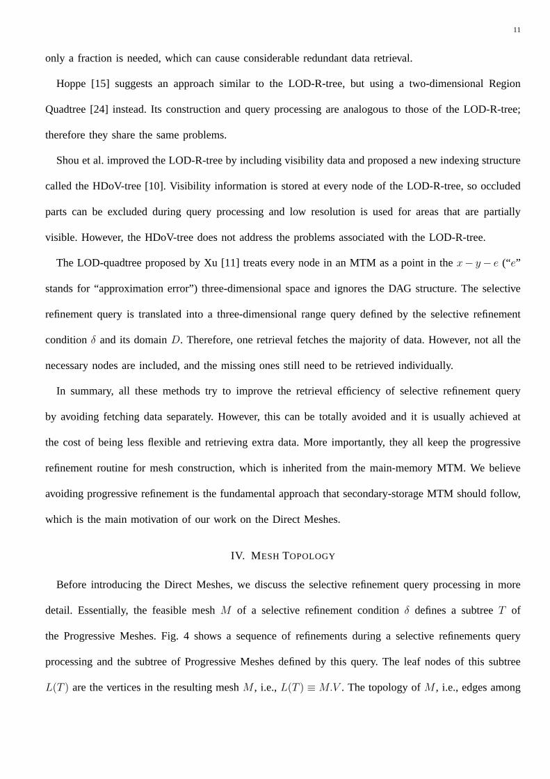
only a fraction is needed, which can cause considerable redundant data retrieval.
Hoppe [15] suggests an approach similar to the LOD-R-tree, but using a two-dimensional Region
Quadtree [24] instead. Its construction and query processing are analogous to those of the LOD-R-tree;
therefore they share the same problems.
Shou et al. improved the LOD-R-tree by including visibility data and proposed a new indexing structure
called the HDoV-tree [10]. Visibility information is stored at every node of the LOD-R-tree, so occluded
parts can be excluded during query processing and low resolution is used for areas that are partially
visible. However, the HDoV-tree does not address the problems associated with the LOD-R-tree.
The LOD-quadtree proposed by Xu [11] treats every node in an MTM as a point in thex− y− e (“e”
stands for “approximation error”) three-dimensional space and ignores the DAG structure. The selective
refinement query is translated into a three-dimensional range query defined by the selective refinement
conditionδ and its domainD. Therefore, one retrieval fetches the majority of data. However, not all the
necessary nodes are included, and the missing ones still need to be retrieved individually.
In summary, all these methods try to improve the retrieval efficiency of selective refinement query
by avoiding fetching data separately. However, this can be totally avoided and it is usually achieved at
the cost of being less flexible and retrieving extra data. More importantly, they all keep the progressive
refinement routine for mesh construction, which is inherited from the main-memory MTM. We believe
avoiding progressive refinement is the fundamental approach that secondary-storage MTM should follow,
which is the main motivation of our work on the Direct Meshes.
IV. M ESH TOPOLOGY
Before introducing the Direct Meshes, we discuss the selective refinement query processing in more
detail. Essentially, the feasible meshM of a selective refinement conditionδ defines a subtreeT of
the Progressive Meshes. Fig. 4 shows a sequence of refinements during a selective refinements query
processing and the subtree of Progressive Meshes defined by this query. The leaf nodes of this subtree
L(T ) are the vertices in the resulting meshM , i.e., L(T ) ≡ M.V . The topology ofM , i.e., edges among
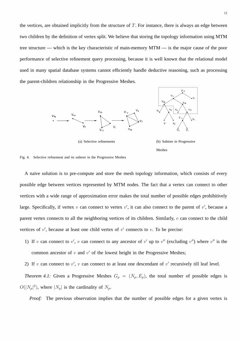
12
the vertices, are obtained implicitly from the structure ofT . For instance, there is always an edge between
two children by the definition of vertex split. We believe that storing the topology information using MTM
tree structure — which is the key characteristic of main-memory MTM — is the major cause of the poor
performance of selective refinement query processing, because it is well known that the relational model
used in many spatial database systems cannot efficiently handle deductive reasoning, such as processing
the parent-children relationship in the Progressive Meshes.
(a) Selective refinements (b) Subtree in Progressive
Meshes
Fig. 4. Selective refinement and its subtree in the Progressive Meshes
A naive solution is to pre-compute and store the mesh topology information, which consists of every
possible edge between vertices represented by MTM nodes. The fact that a vertex can connect to other
vertices with a wide range of approximation error makes the total number of possible edges prohibitively
large. Specifically, if vertexv can connect to vertexv′, it can also connect to the parent ofv′, because a
parent vertex connects to all the neighboring vertices of its children. Similarly,v can connect to the child
vertices ofv′, because at least one child vertex ofv′ connects tov. To be precise:
1) If v can connect tov′, v can connect to any ancestor ofv′ up to v′′ (excludingv′′) wherev′′ is the
common ancestor ofv andv′ of the lowest height in the Progressive Meshes;
2) If v can connect tov′, v can connect to at least one descendant ofv′ recursively till leaf level.
Theorem 4.1:Given a Progressive MeshesGp = (Np, Ep), the total number of possible edges is
O(|Np|2), where|Np| is the cardinality ofNp.
Proof: The previous observation implies that the number of possible edges for a given vertex is
13
proportional to the level of vertices it can connect to, which is proportional to the height of the Progressive
Meshes. Since a Progressive Meshes is an unbalanced binary tree, its height is betweenO(log |Np|) and
O(|Np|). Therefore, the total number of possible edges isO(|Np|2) in the worst case.
A naive method to store all possible edges is not practical due to the substantial storage overhead and
resulting increased I/O costs.
Another option is to encode each node as an MBR (minimum bounding rectangle) of its descendants.
As a result, the MBRs of required nodes intersect with the domain of selective refinement conditionδ.
This, combined with the approximation error range defined byδ, can be used to identify the needed
nodes in MTM. However, the MBRs of the nodes in the upper part of MTM cover a large area and tend
to overlap with each other. Such overlapping can significantly degrade the search performance of most
available spatial access methods, which are based on data partition.
The Direct Meshes only encodes selected topology information, which avoids storing the large amount
of possible edges and can answer a selective refinement query without relying on MTM structure. The
details are elaborated in the next section.
V. D IRECT MESHES
To introduce Direct Meshes, we need to definenode approximation error. Note that this is different
from the vertex approximation error (defined in Section II), which is the absolute difference between the
height of a vertex (φi(vi)) and that of its corresponding vertex in the original model (φ(vn)). In an MTM,
the error introduced by a node should reflect the error of all its descendants, i.e., this vertex accumulates
the distortion that all its descendant nodes bring to the mesh. Therefore, given a Progressive Meshes
Gp = (Np, Ep), the approximation error of noden ∈ Np that represents vertexv is:
e(n) =
0, if n is a leaf node (3)
max(ε(v), e(n.child1), e(n.child2)), otherwise (4)
wheren.child1 andn.child2 are the two children ofn. This definition guarantees that node approximation

14
error value increases monotonically along any path from a leaf to the root.
Another important concept of the Direct Meshes isLOD interval (“LOD” stands for “Level Of Detail”).
For a nodeni ∈ Np, its LOD interval σ(ni) ⊆ R is an interval that
σ(ni) =
[ e(ni), +∞ ), if ni is the root (5)
[ e(ni), e(ni.parent) ), otherwise (6)
whereni.parent is the parent node ofni.
Given a Progressive MeshesGp = (Np, Ep), a Direct MeshesGd = (Np, Ep, Ed) is a multi-relational
graph with an additional relationEd, which is a subset of the cartesian productNp ×Np. Specifically:
Ed = {(ni, nj) | ni, nj ∈ Np, i 6= j, ni ∼ nj, σ(ni) ∩ σ(nj) 6= ∅}
whereni ∼ nj denotes thatni can connect tonj. Ed is the set of possible edges whose end nodes have
overlapping LOD intervals. We name themcandidate edges. The candidate edge set is a subset of all
possible edges, and its size is much less than that of the latter because the LOD-interval-overlapping
constraint limits the number of different resolution levels a candidate edge can cross. In fact, the average
number of candidate edges for each node is a constant (proof is given later in this section). Thus, the size
of Ed is linear to the number of nodesO(|Np|).
Each node of a Direct Meshes has the following data structure:
ClassDirectMeshNode{
Integer NodeID;
Doublex, y, z;
Doublee; // node approximation error
DirectMeshNodeparent, child1, child2;
DirectMeshNodeArrayNb; // the other end node of candidate edges
}

15
Algorithm 2 : Direct Meshes Construction
Input : Progressive MeshesGp = (Np, Ep)
Output : Direct MeshesGd = (Np, Ep, Ed), every noden ∈ Np has a list of candidate edgesNb
Ne ← the ordered set of all nodes inNp with a descending approximation error (ancestor is ahead1
of descendant if they have the same error) ;
while Ne is not emptydo2
n0 ← the first node inNe;3
removen0 from Ne;4
if n0.parent 6= null then5
n1 ← the other child node ofn0.parent;6
n0.Nb ← n0.Nb ∪ {n1} ;7
for every nodeni ∈ n0.parent.Nb do8
if n0.Nb ∩ {ni} = ∅ AND σ(ni) ∩ σ(n0) 6= ∅ AND ni ∼ n0 then9
n0.Nb ← n0.Nb ∪ {ni} ;10
Ndi ← the set of descendent nodes ofni whose LOD interval overlaps with that ofn0;11
for every nodendj ∈ Nd
i do12
if n0.Nb ∩ {ndj} = ∅ AND ni ∼ n0 then13
n0.Nb ← n0.Nb ∪ {ndj} ;14
endif15
endfor16
endif17
endfor18
endif19
endw20
Algorithm 2 outlines the major steps of the Direct Meshes construction. The algorithm scans the node
16
setNp in a descending-approximation-error order and finds the candidate edge setNb for every node. It
starts with ordering the nodes according to their approximation error (line 1). For every noden, the first
candidate edge is the one between itself and the node sharing the same parent (line 5-7). To find other
candidate edges, the algorithm checks the nodes in the parent candidate edge set and their descendants
(line 8-18). For algorithm correctness proof, we need the following lemma:
Lemma 5.1:Given a noden and its candidate edge listn.Nb, n′ (the parent node ofn) and its candidate
edge listn′.Nb, for every nodeni ∈ n.Nb (except the node (n0) sharing the same parent),ni ∈ n′.Nb or
there is a noden′i ∈ n′.Nb such thatn′i is an ancestor ofni.
Proof: First, we show that for a nodeni, if ni ∼ n, thenni ∼ n′. Becauseni ∼ n, we can construct
a mesh that has(ni, n) as one of its edge and(n, n0) as another edge. Then, we can simplify the mesh
by collapsing edge(n, n0) into n′. There will be an edge(ni, n′) in the new mesh, thereforeni ∼ n′.
This can be extended to any ancestor ofn, i.e., n′′ ∼ ni if n ∼ ni andn′′ is an ancestor ofn.
For a nodeni ∈ n.Nb, ni ∼ n, thereforeni ∼ n′. If σ(ni) ∩ σ(n) 6= ∅, ni ∈ n.Nb, proved. Otherwise,
e(ni.parent) < e(n′) becauseσ(ni) ∩ σ(n) = ∅ and e(n) ≤ e(n′). Let n′i be one of the ancestors
of ni. Becauseni ∼ n′, n′i ∼ n′. Becausee(n′i) ≥ e(ni), there is always an ancestorn′i such that
σ(n′i) ∩ σ(n′) 6= ∅, thereforen′i ∈ n′.Nb, proved.
Theorem 5.1:Algorithm 2 finds all the candidate edges in a Progressive Meshes.
Proof: To prove this, it is sufficient to show that the algorithm finds all the candidate edges for
every node. The root is the only node that has no parent. It is obvious that the root has no candidate edge,
because the only possible mesh that has the root is the one that has the root as the only vertex. Except
the root, every node has a parent. From Lemma 5.1 we know all the candidate edges of a node can be
found by searching the nodes in its parent candidate edge set and their descendants. The ordering of the
nodes guarantees that parent candidate edges are always computed before that of its children. Therefore,
the algorithm finds all the candidate edges for every node.
Next, we discuss the time complexity and storage requirement of the algorithm, which requires the

17
following lemmas.
Lemma 5.2:Given two intervalsA,B ⊆ R that are both partitioned into a set of sub-intervals, i.e.,
A = ∪mk=1ak, ai ∩ aj = ∅, i 6= j, 1 ≤ i, j ≤ m
B = ∪nk=1bk, bi ∩ bj = ∅, i 6= j, 1 ≤ i, j ≤ n
For 1 ≤ i ≤ m, 1 ≤ j ≤ n, there is ainterval edge(ai, bj) if ai ∩ bj 6= ∅. The maximum total number
of interval edges (max(|Ei|)) is m + n− 1.
Proof: This can be proved by induction.
• Base case:m = 1, n = 1. |Ei| = 0 whenA ∩B = ∅; |Ei| = 1 otherwise. Therefore,max(|Ei|) = 1
• Inductive step: assume thatmax(|Ei|) = k − 1 whenm + n = k.
Let m+n = k+1. Without loss of generality, we assume that the increased partition is introduced by
dividing an existing partitionai ⊂ A at pointp. It is obvious that|Ei| will not change if{p}∩B = ∅;
|Ei| will increase by 1 otherwise. Thereforemax(|Ei|) = (k − 1) + 1 = k.
Based on Lemma 5.2, we have the following lemma.
Lemma 5.3:Given a Direct MeshesGd = (Np, Ep, Ed), the total number of candidate edges|Ed| is
O(|Np|).
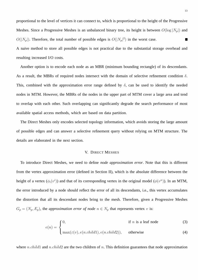
Proof: The Progressive MeshesGp = (Np, Ep), which is a binary tree, can be divided into a set
of paths whose approximation error changes monotonically. For instance, Fig. 5 shows a partition of the
Progressive Meshes in Fig. 4(b) into a set of such paths. Every path is an approximation error interval that
is the union of the LOD interval of every node. For example the left-most path is an error interval[0, +∞)
and it is the union of the LOD interval ofv15 ( [e(v15), +∞) ), v14 ( [e(v14), e(v15)) ), etc. According to
Lemma 5.2, the total number of candidate edges, which is equivalent to interval edge, is linear to the
total number of interval partitions, which in this case equals|Np|.
However, each path can be paired with more than one other path. If we take any mesh that can be
constructed fromGp, the average node degree is constant because it is a triangulation. In other words, on
18
average one path can pair with a constant number of paths. Thus, the total number of interval edges is
k ·Np wherek is a constant, i.e., the total number of candidate edges isO(|Np|).
Fig. 5. Partition of a Progressive Meshes into a set of paths
Given the Lemma 5.3, we have the following theorem.
Theorem 5.2:Given a Progressive MeshesGp = (Np, Ep), the running time of Algorithm 2 isO(|Np|)
and it requiresO(|Np|) space for the candidate edge set of the resulting Direct Meshes.
Proof: The algorithm starts with sorting all the nodes inNp according to their approximation error.
Because the error decreases monotonically along any path from the root to leaf, this can be done in
O(|Np|) time. Within the main loop (line 2-20), removing the first noden0 from the sorted node setNe
takes constant time (line 3-4). It is the same for finding the noden1 sharing the same parent (line 6-7),
given that every node stores links to its parent and children. From Lemma 5.3, we know on average every
node has a constant number of candidate edges, therefore the next loop (line 8-18) repeats a constant
time. Similarly, we can show that the average node number inNdi (line 11) is also constant. Thus, the
next loop (line 12-15) runs in constant time. Therefore, the running time of Algorithm 2 isO(|Np|). From
Lemma 5.3 we know there areO(|Np|) candidate edges in total, so it requiresO(|Np|) space.
In summary, the Direct Meshes requires no modification to the original MTM structure; it adds an
candidate edge set for every node, which can be done in linear time with linear space. Selective refinement
query processing using the Direct Meshes is discussed in the next section.
19
VI. SELECTIVE REFINEMENT QUERY PROCESSING
Once the Direct Meshes is constructed, an important issue is the choice of spatial access method,
which needs to support the characteristics of the Direct Meshes database and selective refinement query.
As mentioned in [11], the distribution of MTM nodes in thex-y-e three-dimensional space is highly
skewed, which makes it unsuitable for spatial access methods based on regular space partition, such as
Region Quadtree [24]. As we will see later in this section, selective refinement query can be converted
to range query inx-y-e space, which makes it unnecessary for any particular method to support graph
traversing (the Direct Meshes is essentially a DAG), such as the connectivity-clustered access method
[25]. The results in [26] showed that the R-tree and the R+-tree have much better query performance than
the K-D-B-tree [27] when the datasets contain rectangles of varying size, which is very similar to the
case of selective refinement query (as we shall see later in this section). We did not use variations of Grid
File, such as the Multilevel Grid File [28], as they share a similar indexing structure as the K-D-B-tree.
Eventually, we choose the R*-tree [29] because it is reported to have the best performance among the
R-tree variations [29]. Every noden in a Direct Meshes is indexed using a R*-tree as a three-dimensional
line segment
((n.x, n.y, e(n)), (n.x, n.y, e(n.parent))
representing its LOD interval in thex− y − e space.
Given a Direct MeshesGd = (Np, Ep, Ed) and a selective refinement conditionδ (with domainD),
Algorithm 3 outlines the main steps of processing the queryQ(Gd, δ). The algorithm retrieves all the
nodes withinD and having an LOD interval that overlaps with the error interval(δmin, δmax) defined by
the selective refinement conditionδ (line 2). Thebase meshM0 is then built according to the selective
refinement conditionδ′ : D → δmax (line 3-11). M0 is further refined using the Algorithm 1 until the
required meshM is obtained. Note that only one retrieval is performed (line 2) and it fetches all the data
used by the algorithm.

20
Algorithm 3 : Selective refinement using Direct MeshesInput : Direct MeshesGd = (Np, Ep, Ed), selective refinement conditionδ
Output : meshM that is feasible regarding toδ
δmin/δmax ← the minimal / maximal approximation error value defined byδ over domainD;1
N ← set of nodes that are withinD and their LOD interval overlaps with(δmin, δmax);2
N0 ← set of nodes that are withinD and their LOD interval containsδmax;3
MeshM0 = (N0, E0), E0 ← ∅;4
for every nodeni ∈ N0 do5
for every nodenj ∈ ni.Nb do6
if nj ∈ N0 AND E0 ∩ {(ni, nj)} = ∅ then7
E0 ← E0 ∪ {(ni, nj)};8
endif9
endfor10
endfor11
MeshM ← Algorithm 1(M0,N );12
return M ;13
Theorem 6.1:Given a Direct MeshesGd = (Np, Ep, Ed), the meshM returned by Algorithm 3 is
feasible for the selective refinement conditionδ.
Proof: First, we show that meshM0 produced by the algorithm is a proper mesh. For every node
ni ∈ N0, its LOD interval containsδmax, therefore their LOD intervals all overlap with each other. Because
the Direct Meshes contains every possible candidate edge andE0 is a subset ofEd, then every edge in
E0 is contained in the candidate edge list of nodes inN0. Since all the nodes have overlapping LOD
intervals, meshM0 should be checked during the Direct Meshes construction. Any candidate edge that
may breach the validity of a mesh (such as causing an improper triangulation) should be excluded from
the Direct Meshes. Therefore, every candidate edge inE0 is necessary forM0. Thus, M0 is a proper

21
mesh. OnceM0 is constructed, it is further refined by Algorithm 1, which is proved in the previous work
to produce the feasible mesh for the given selective refinement conditionδ.
A. Cost Analysis
The I/O cost of processing a selective refinement query using the Direct Meshes can be modeled as:
DA(Q) = I + t0 · d|N |/Be (7)
whereI is the cost of searching the R*-tree of the Direct Meshes to find the required nodes,t0 is the
cost of retrieving one disk page,|N | is the total number of nodes needed, andB is the number of nodes
each disk page can hold. Here we assume that the required nodes are stored continuously on the disk.
Although this cannot be fully achieved in practice, it can be seen as a close estimation of the real cost.
Similarly, the cost of previous methods can be modeled as:
DA(Q) = (I ′ + k · t0) · d|N ′|/(k ·B)e (8)
wherek is a nature number and indicates the node size of the indexing structure, because these methods
with customized index can have node size more than one disk page.
From the cost models we can see that the Direct Meshes incurs less I/O cost than the previous methods:
1) Less index scan. While index scan only occurs once using the Direct Meshes,d|N ′|/(k ·B)e scans
are needed previously because one is needed for every retrieval of child nodes during progressive
refinement.
2) Less redundant data. A node could contain unnecessary data, especially when the area it covers is
on the boundary of the domainD. Though this is unavoidable, the smaller the index node size, the
less the redundant data. The Direct Meshes, which have the minimal index node size one, retrieve
less redundant data than previous methods (index node sizek) when answering the same query.
3) Less MTM node retrieval. Previous methods always start from the MTM root to find the feasible
mesh; whereas the Direct Meshes can start from the lowest mesh resolution (δmax) and skip all
22
the MTM nodes with lower resolution. The saving can be significant, especially when the required
mesh has a uniform resolution.
B. Query Optimization
The Direct Meshes works best when the selective refinement conditionδ specifies a constantδ0 overD,
in which case the base meshM0 is feasible and no redundant data is retrieved. Whenδ is not a constant,
we consider the case that the required resolution reduces linearly to the vertex distance to a reference
(such as the viewpoint). Such selective refinement produces a uniform resolution mesh on display (Fig.
2), and is arguably the most common query in multi-resolution visualization. Specifically, for a vertex
v ∈ D its required resolution valueδ(v) is:
δ(v) = δ0 − k · | v − τ0| (9)
wherek is a constant and| v − τ0| is the Euclidean distance betweenv and the referenceτ0. In this case
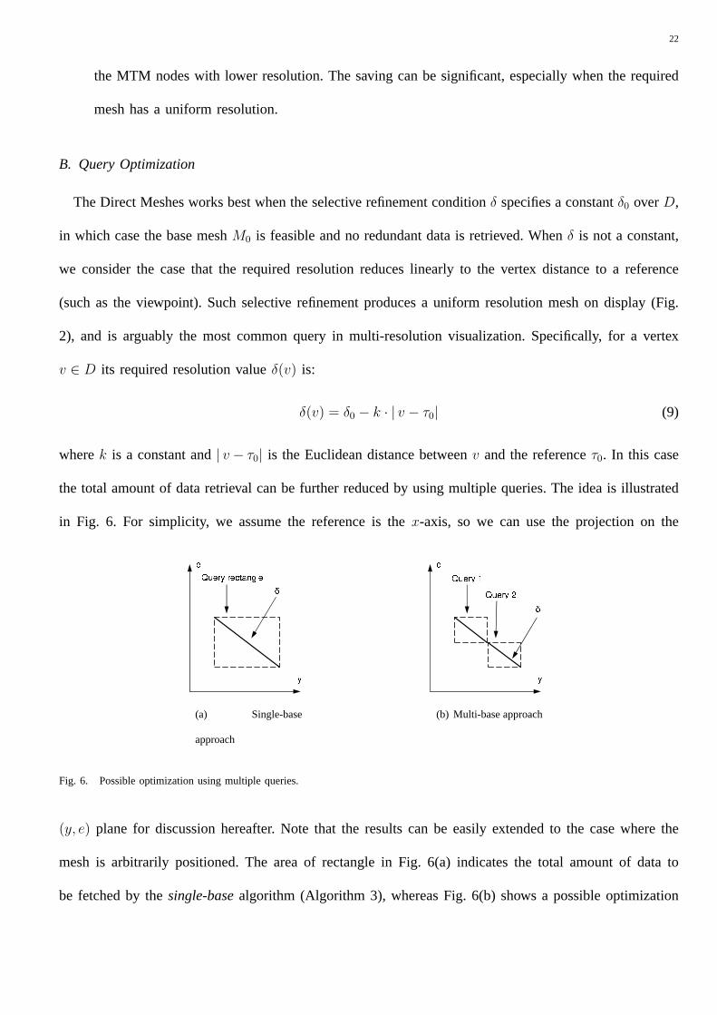
the total amount of data retrieval can be further reduced by using multiple queries. The idea is illustrated
in Fig. 6. For simplicity, we assume the reference is thex-axis, so we can use the projection on the
(a) Single-base
approach
(b) Multi-base approach
Fig. 6. Possible optimization using multiple queries.
(y, e) plane for discussion hereafter. Note that the results can be easily extended to the case where the
mesh is arbitrarily positioned. The area of rectangle in Fig. 6(a) indicates the total amount of data to
be fetched by thesingle-basealgorithm (Algorithm 3), whereas Fig. 6(b) shows a possible optimization
23
using two queries. In the latter case the total data retrieval amount (indicated as the sum of the area
of two query rectangles) is less than that of using one query only (Fig. 6(a)). However, themulti-query
approach has its own overhead such as the cost of index scan for each query. Therefore, to minimize
the overall retrieval, the optimization algorithm should partition the domainD into a set of sub-domains
S(D) = {d1, d2, . . . , dn} so that the total retrieval costDA(D) = DA(d1) + DA(d2) + . . . + DA(dn) is
minimized. In practice, it is difficult to find the optimal partitionS(D) that minimized the retrieval cost.
Here we propose a heuristic approach that partitions the domain recursively, based on the retrieval cost
estimation.
The problem of analyzing the I/O cost of range queries using the R-tree and its variants has been
extensively studied in the past ([30], [31], [32], [33], [34], [35]). The number of disk accesses (DA) using
a three-dimensional R-tree indexTr with Nr nodes to process a range queryq can be estimated using the
following formula [32], [33]:
DA(Tr, q) =Nr∑i=1
(qx + wi) · (qy + hi) · (qz + di) (10)
whereqx, qy andqz are the width, height and depth of the query cube respectively, andwi, hi anddi are
the width, height and depth of nodeni of Tr respectively. All the values are normalized according to the
data space, which has a unit size (1× 1× 1). The value ofDA(Tr, q) includes the I/O cost of both index
scan and data retrieval. Formula (10) provides an estimation of I/O cost for single-base approach (Fig.
6(a)); when two queries are used (Fig. 6(b)), the total costDA′(Tr, q) is:
DA′(Tr, q) =Nr∑i=1
(qx1 + wi) · (qy1 + hi) · (qz1 + di) +Nr∑i=1
(qx2 + wi) · (qy2 + hi) · (qz2 + di) (11)
whereqx1, qy1, qz1 andqx2, qy2, qz2 are the width, height and depth of the two query cubes respectively.
More queries should be used only if it incurs less total I/O cost, i.e.,
DA(Tr, q)−DA′(Tr, q) > 0 (12)
24
From Fig. 6, we have:
qx = qx1 = qx2 (13)
qy = qy1 + qy2 (14)
qz = qz1 + qz2 (15)
Note that formula (13) to (15) still holds if the query plane is not parallel to thex-axis, because this
change only affects the position of the query plane, not its size. Combining (10)-(15), we have:
Nr∑i=1
(qx1 + wi)(qyqz − (qy1qz1 + qy2qz2)− hidi) > 0 (16)
i.e., so long as condition (16) holds, more queries should be used. As the size of the R-tree nodes (hi,
di, wi) can be obtained from the R-tree index, all the data required for this optimization is available.
From formula (16), we can know that the maximum reduction can be achieved when the value below is
maximized:
qy · qz − (qy1 · qz1 + qy2 · qz2) (17)
This gives the area difference between the rectangle of the single-base case (Fig. 5(a)) and the sum of
the area of the rectangles of the multi-base case (Fig. 5(b)). Asqy and qz are given by the query,qy · qz
is a constant. Therefore:
qy1 · qz1 + qy2 · qz2 (18)
is the only variable element. To maximize the value of (17), the value of (18) should be minimized,
which means that dividing the original query into two equal-sized sub-queries will give the maximum
I/O reduction. Given a Direct MeshesGd = (Np, Ep, Ed), its R*-tree indexTr, and a selective refinement
condition δ, Procedure “SelectiveRefinement-MultiBase” outlines the main steps of a query processing
algorithm that adopts the multi-base approach.
25
Procedure SelectiveRefinement-MultiBase( Gd, Tr, δ)
MeshM ← ∅;1
D1, D2 ← the two partitions result from dividingD equally;2
if DA(D1) + DA(D2) < DA(D) then3
MeshM1 ← SelectiveRefinement-MultiBase(D1);4
MeshM2 ← SelectiveRefinement-MultiBase(D2);5
M ← M1 + M2;6
else7
M ← Algorithm3(Gd, δ(D));8
endif9
return M ;10
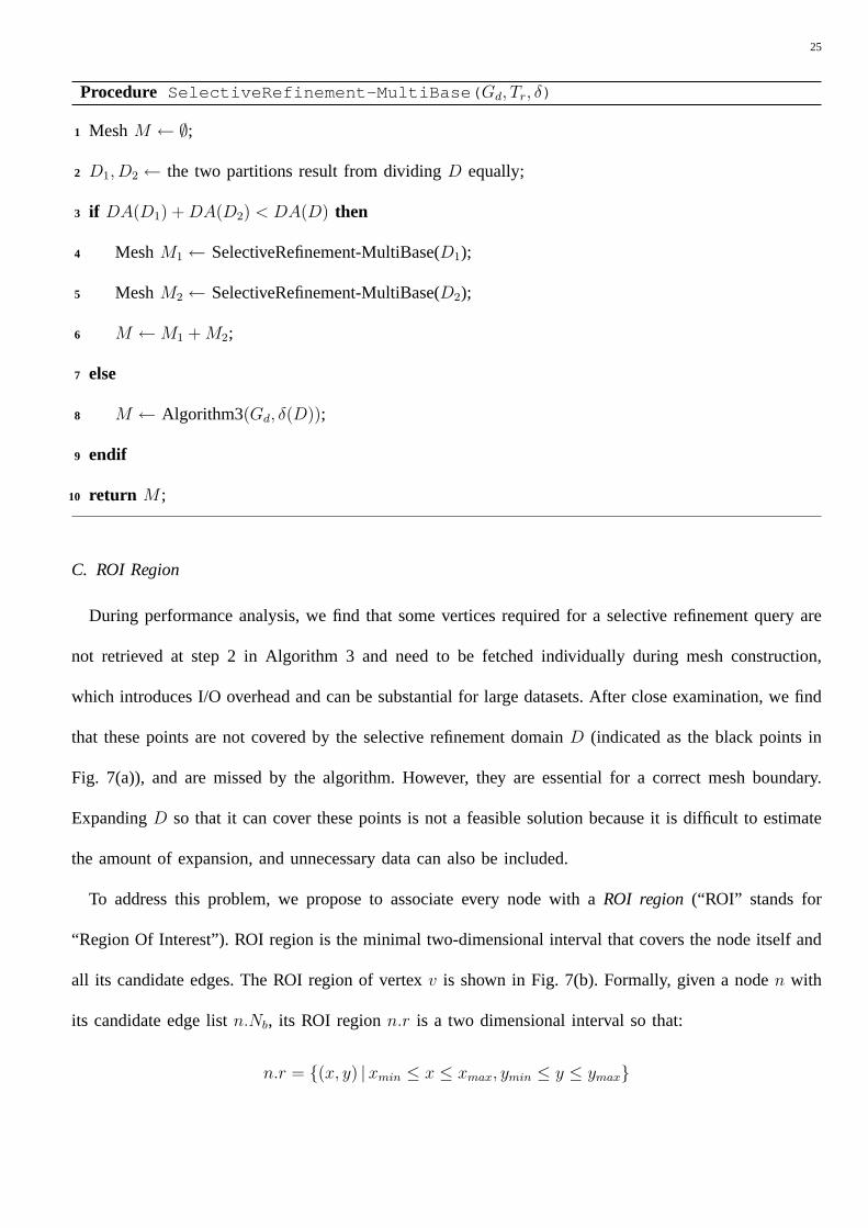
C. ROI Region
During performance analysis, we find that some vertices required for a selective refinement query are
not retrieved at step 2 in Algorithm 3 and need to be fetched individually during mesh construction,
which introduces I/O overhead and can be substantial for large datasets. After close examination, we find
that these points are not covered by the selective refinement domainD (indicated as the black points in
Fig. 7(a)), and are missed by the algorithm. However, they are essential for a correct mesh boundary.
ExpandingD so that it can cover these points is not a feasible solution because it is difficult to estimate
the amount of expansion, and unnecessary data can also be included.
To address this problem, we propose to associate every node with aROI region (“ROI” stands for
“Region Of Interest”). ROI region is the minimal two-dimensional interval that covers the node itself and
all its candidate edges. The ROI region of vertexv is shown in Fig. 7(b). Formally, given a noden with
its candidate edge listn.Nb, its ROI regionn.r is a two dimensional interval so that:
n.r = {(x, y) |xmin ≤ x ≤ xmax, ymin ≤ y ≤ ymax}
26
(a) ROI feasible points that
are outside ROI
(b) ROI region ofv
b
Fig. 7. ROI region
where:
• xmin = min(n.x, ni.x |ni ∈ n.Nb);
• xmax = max(n.x, ni.x |ni ∈ n.Nb);
• ymin = min(n.y, ni.y |ni ∈ n.Nb);
• ymax = max(n.y, ni.y |ni ∈ n.Nb);
ROI region can be computed in constant time once all the candidate edges are identified; therefore including
ROI region will not change the running time of the Direct Meshes construction algorithm. Also, each
node requires constant space for an ROI region, thus it will not change the storage requirement of the
Direct Meshes.
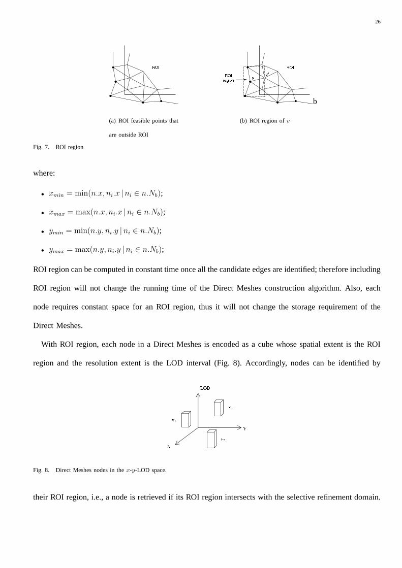
With ROI region, each node in a Direct Meshes is encoded as a cube whose spatial extent is the ROI
region and the resolution extent is the LOD interval (Fig. 8). Accordingly, nodes can be identified by
Fig. 8. Direct Meshes nodes in thex-y-LOD space.
their ROI region, i.e., a node is retrieved if its ROI region intersects with the selective refinement domain.
27
This is the only modification required for the query processing algorithm (Algorithm 3).
VII. PERFORMANCEEVALUATION
In this section, we evaluate the performance of the selective refinement query processing based on the
Direct Meshes. Two different versions of the Direct Meshes are implemented: one does not apply “ROI
region” (as described in Section V); the other does (as described in Section VI). Both Direct Meshes have
a three-dimensional R∗-tree built upon them for query processing. For comparison we also include the
LOD-quadtree and the HDoV-tree, because they provide the best performance among the available methods
that support MTM with DAG structure. The Progressive Meshes is implemented as described in [21]. The
LOD-quadtree is created according to [11]. The HDoV tree is constructed following the algorithms in
[10]. For the HDoV tree, the terrain is partitioned into grids, which serve as the objects in the HDoV tree.
Visibility data is stored using the “indexed-vertical storage scheme”, which is reported to have the best
performance among the proposed schemes for the HDoV-tree. Two types of selective refinement queries
are tested: one is theuniform-LOD querywhere the selective refinement condition specifies a constant
value over its domain, the other is thevariable-LOD querywhere the selective refinement condition
specifies a value reducing linearly to the vertex distance. For the latter, the test results of both single-base
and multi-base methods are included.
The total cost of the MTM query processing is composed of two parts: the cost of data access (I/O
cost) and the cost of mesh construction (CPU cost). In terms of running time, it is found that the former
dominates the overall cost. Therefore, we focus our performance evaluation on the I/O cost, which is
measured by the number of disk accesses (obtained from Oracle’s performance statistics report). Note
that the CPU cost of the Direct Meshes is generally smaller than that of the other two methods due to the
fact that it retrieves less data, and thus requires less computation for refinement, if there is any. All the
values in the results are the average value of repeating the same query at 20 randomly-selected locations.
Terrain data is arranged on the disk in such a way that their(x, y) clustering is preserved as much as
possible.

28
We use Oracle Enterprise Edition Release 9.0.1 in our tests. Its object-relational features and the Oracle
Spatial Option are not used in order to have a better control and understanding of the query execution
performance. All spatial indexes used are implemented by ourselves. B+-tree indexes are created wherever
necessary. The database and system buffer is flushed before each test to minimize the effect of caching.
Other software packages used are Java SDK 1.3 (for data retrieval) and Java3D SDK (openGL) 1.2 (for
mesh visualization). The hardware used is a Pentium III 700 with 512MB memory. Two real-world terrain
datasets are used in the tests. The first one is a 2-million-point terrain model from a local mining software
company. The second dataset is the DEM model of “Crater Lake National Park” from U.S. Geological
Survey (www.usgs.gov) with 17 million points.
A. Uniform-LOD Query Performance
The two main parameters that affect the performance of the uniform-LOD queries are the resolution
value specified by the selective refinement condition and the size of its domain. Generally, the I/O cost
increases as the resolution value decreases (which implies a more detailed mesh) or the domain size
increases. To separate their effects we conducted two sets of tests. The first set has varying domain size
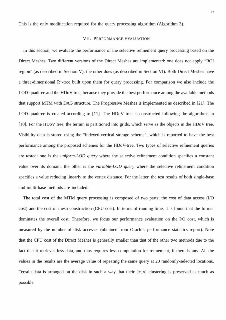
and fixed resolution value, whereas the second set is the opposite. Figures 9(a) and 9(c) show the results
of the first set with 2 and 17 million points respectively. Thex-axis measures the domain size (indicated
as “ROI”), shown as the percentage of the dataset area, andy-axis measures the number of disk accesses.
The mesh resolution is set to the average value of the dataset, and the range of domain size is chosen to
allow for a mesh with reasonable data density when displayed, i.e., avoid meshes that are overly crowded
when displayed. The LOD-quadtree is indicated as “PM” (stands for “Progressive Meshes” because it
does not change its structure), the HDoV tree as “HDoV”, and the Direct Meshes as “SB” (single-base
method). Similarly, figures 9(b) and 9(d) show the results of the second set. Thex-axis denotes resolution
(indicated as “LOD”), shown as the percentage of maximum LOD value in the dataset. The domain size
is set to 10% for the 2M dataset and 5% for the 17M dataset. We include the results of a resolution
range that contains a substantial number of points. Performance changes are hardly noticeable when the
29
resolution value is beyond this range.
(a) Varying ROI - 2M dataset (b) Varying LOD - 2M dataset (c) Varying ROI - 17M dataset (d) Varying LOD - 17M dataset
Fig. 9. Uniform mesh.
The Direct Meshes clearly outperforms the other two methods in these tests, and the performance gap
grows as the mesh size increases. This complies well with our analysis in Section VI, since the Direct
Meshes incurs much less retrieval overhead than the other two methods. The slow increase of the Direct
Meshes also indicates that it scales much better with the mesh size than the other two.
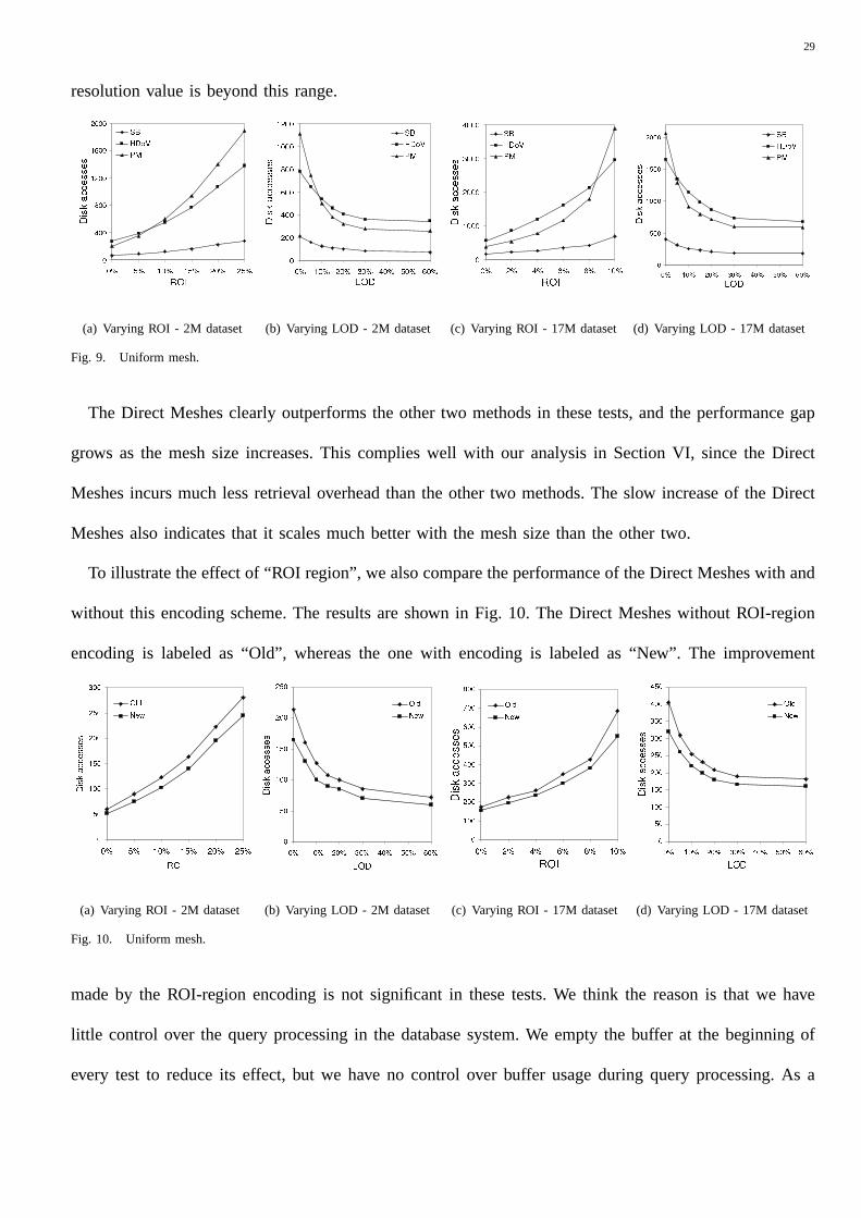
To illustrate the effect of “ROI region”, we also compare the performance of the Direct Meshes with and
without this encoding scheme. The results are shown in Fig. 10. The Direct Meshes without ROI-region
encoding is labeled as “Old”, whereas the one with encoding is labeled as “New”. The improvement
(a) Varying ROI - 2M dataset (b) Varying LOD - 2M dataset (c) Varying ROI - 17M dataset (d) Varying LOD - 17M dataset
Fig. 10. Uniform mesh.
made by the ROI-region encoding is not significant in these tests. We think the reason is that we have
little control over the query processing in the database system. We empty the buffer at the beginning of
every test to reduce its effect, but we have no control over buffer usage during query processing. As a
30
result, the cost of individually retrieving necessary nodes outside selective refinement condition domain
is considerably reduced, because the index scanning associated with such retrieval is very likely to be
performed in the buffer with considerably reduced cost. Nevertheless, the new encoding scheme still
achieves reasonable reduction on retrieval cost.
B. Variable-LOD Query Performance
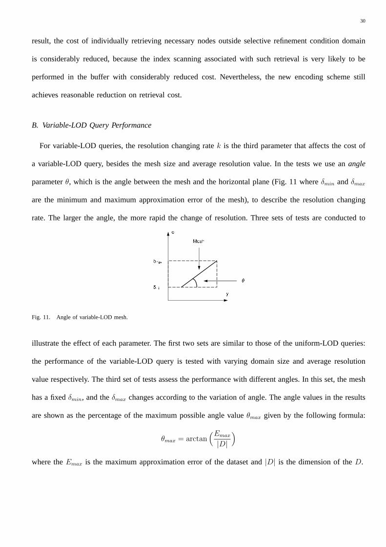
For variable-LOD queries, the resolution changing ratek is the third parameter that affects the cost of
a variable-LOD query, besides the mesh size and average resolution value. In the tests we use anangle
parameterθ, which is the angle between the mesh and the horizontal plane (Fig. 11 whereδmin andδmax
are the minimum and maximum approximation error of the mesh), to describe the resolution changing
rate. The larger the angle, the more rapid the change of resolution. Three sets of tests are conducted to
Fig. 11. Angle of variable-LOD mesh.
illustrate the effect of each parameter. The first two sets are similar to those of the uniform-LOD queries:
the performance of the variable-LOD query is tested with varying domain size and average resolution
value respectively. The third set of tests assess the performance with different angles. In this set, the mesh
has a fixedδmin, and theδmax changes according to the variation of angle. The angle values in the results
are shown as the percentage of the maximum possible angle valueθmax given by the following formula:
θmax = arctan(Emax
|D|)
where theEmax is the maximum approximation error of the dataset and|D| is the dimension of theD.
31
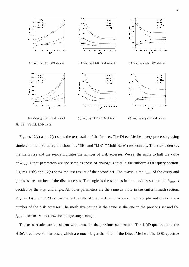
(a) Varying ROI - 2M dataset (b) Varying LOD - 2M dataset (c) Varying angle - 2M dataset
(d) Varying ROI - 17M dataset (e) Varying LOD - 17M dataset (f) Varying angle - 17M dataset
Fig. 12. Variable-LOD mesh.
Figures 12(a) and 12(d) show the test results of the first set. The Direct Meshes query processing using
single and multiple query are shown as “SB” and “MB” (“Multi-Base”) respectively. Thex-axis denotes
the mesh size and they-axis indicates the number of disk accesses. We set the angle to half the value
of θmax. Other parameters are the same as those of analogous tests in the uniform-LOD query section.
Figures 12(b) and 12(e) show the test results of the second set. Thex-axis is theδmin of the query and
y-axis is the number of the disk accesses. The angle is the same as in the previous set and theδmax is
decided by theδmin and angle. All other parameters are the same as those in the uniform mesh section.
Figures 12(c) and 12(f) show the test results of the third set. Thex-axis is the angle andy-axis is the
number of the disk accesses. The mesh size setting is the same as the one in the previous set and the
δmin is set to 1% to allow for a large angle range.
The tests results are consistent with those in the previous sub-section. The LOD-quadtree and the
HDoV-tree have similar costs, which are much larger than that of the Direct Meshes. The LOD-quadtree
32
retrieves substantially more data than the Direct Meshes, which is the main cause of its poor performance.
Visibility selection does not help the HDoV-tree much because obstruction among the areas of the tested
terrain is not as much as in the synthetic city model described in [10]. Hence, the visibility constraint
does not always significantly reduce data amount. The multi-base approach performs best. Its comparison
against the single-base method shows that the optimization can significantly reduce retrieval cost. Note
that the performance of approaches based on the Direct Meshes decreases as the angle increases (Fig.
12(c) and 12(f)). The reason is that the increase of angle implies a bigger difference between theδmin
andδmax; thus, a larger query cube for single-base method (similar to multi-base method) as theδmin is
fixed. However, even the single-base method still has a considerable performance advantage against the
other two methods.
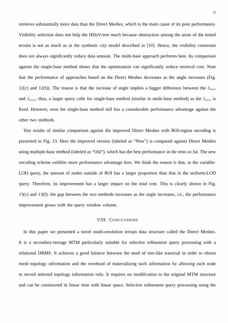
Test results of similar comparison against the improved Direct Meshes with ROI-region encoding is
presented in Fig. 13. Here the improved version (labeled as “New”) is compared against Direct Meshes
using multiple-base method (labeled as “Old”), which has the best performance in the tests so far. The new
encoding scheme exhibits more performance advantage here. We think the reason is that, in the variable-
LOD query, the amount of nodes outside of ROI has a larger proportion than that in the uniform-LOD
query. Therefore, its improvement has a larger impact on the total cost. This is clearly shown in Fig.
13(c) and 13(f): the gap between the two methods increases as the angle increases, i.e., the performance
improvement grows with the query window volume.
VIII. C ONCLUSIONS
In this paper we presented a novel multi-resolution terrain data structure called the Direct Meshes.
It is a secondary-storage MTM particularly suitable for selective refinement query processing with a
relational DBMS. It achieves a good balance between the need of tree-like traversal in order to obtain
mesh topology information and the overhead of materializing such information by allowing each node
to record selected topology information only. It requires no modification to the original MTM structure
and can be constructed in linear time with linear space. Selective refinement query processing using the
33
(a) Varying ROI - 2M dataset (b) Varying LOD - 2M dataset (c) Varying angle - 2M dataset
(d) Varying ROI - 17M dataset (e) Varying LOD - 17M dataset (f) Varying angle - 17M dataset
Fig. 13. Variable-LOD mesh.
Direct Meshes improves the performance by avoiding multiple retrievals and reducing the total amount of
required data. The multi-base approach further reduces the cost of varying-LOD queries. The introduction
of ROI region encoding provides a solution for retrieving necessary data outside of the selective refinement
condition domain. Significant performance improvement is observed from tests based on the real-world
datasets. The scalability of the Direct Meshes is demonstrated when comparing against best available
methods with different data sizes.
REFERENCES
[1] W. Piekarski and B. Thomas, “Arquake: the outdoor augmented reality gaming system,”Communications of the ACM, vol. 45, no. 1,
pp. 36–38, 2002.
[2] M. C. Whitton, “Making virtual environments compelling,”Communications of the ACM, vol. 46, no. 7, pp. 40 – 47, 2003.
34
[3] D. Green, J. Cosmas, T. Itagaki, M. Waelkens, R. Degeest, and E. Grabczewski, “A real time 3D stratigraphic visual simulation system
for archaeological analysis and hypothesis testing,” inConference on Virtual Reality, Archeology, and Cultural Heritage. Glyfada,
Greece: ACM Press, 2001, pp. 271 – 278.
[4] S. Kiss and A. Nijholt, “Viewpoint adaptation during navigation based on stimuli from the virtual environment,” inEighth International
Conference On 3D Web Technology. Saint Malo, France: ACM Press, 2003, pp. 19 – 26.
[5] B. Benes and R. Forsbach, “Parallel implementation of terrain erosion applied to the surface of mars,” in1St International Conference
on Computer Graphics, Virtual Reality and Visualisation. Camps Bay, Cape Town, South Africa: ACM Press, 2001, pp. 53 – 57.
[6] T. Gerstner, D. Meetschen, S. Crewell, M. Griebel, and C. Simmer, “A case study on multiresolution visualization of local rainfall
from weather radar measurements,” inConference on Visualization. Boston, Massachusetts: IEEE Computer Society, 2002, pp. 533
– 536.
[7] J. Randall W. Hill, Y. Kim, and J. Gratch, “Anticipating where to look: predicting the movements of mobile agents in complex terrain,”
in International Joint Conference on Autonomous Agents and Multiagent Systems. Bologna, Italy: ACM Press, 2002, pp. 821 – 827.
[8] B. Ben-Moshe, J. S. B. Mitchell, M. J. Katz, and Y. Nir, “Visibility preserving terrain simplification: an experimental study,” in
Eighteenth Annual Symposium on Computational Geometry. Barcelona, Spain: ACM Press, 2002, pp. 303 – 311.
[9] M. Garland, “Multiresolution modeling: Survey & future opportunities,” inEurographics ’99 – State of the Art Reports. Aire-la-Ville
(CH), 1999, pp. 111–131.
[10] L. Shou, Z. Huang, and K.-L. Tan, “HDoV-tree: The structure, the storage, the speed,” in19th International Conference on Data
Engineering (ICDE) 2003, Bangalore, India, 2003, pp. 557–568.
[11] K. Xu, “Database support for multiresolution terrain visualization,” inThe 14th Australian Database Conference, ADC 2003. Adelaide,
Australia: Australian Computer Society, 2003, pp. 153–160.
[12] C. DeCoro and R. Pajarola, “Xfastmesh: fast view-dependent meshing from external memory,” inConference on Visualization. Boston,
Massachusetts: IEEE Computer Society, 2002, pp. 363 – 370.
[13] P. Lindstrom, “Out-of-core construction and visualization of multiresolution surfaces,” inSymposium on Interactive 3D graphics.
Monterey, California: ACM Press, 2003, pp. 93 – 102.
[14] M. Isenburg and S. Gumhold, “Out-of-core compression for gigantic polygon meshes,”ACM Transactions on Graphics, vol. 22, no. 3,
pp. 935 – 942, 2003.
[15] H. Hoppe, “Smooth view-dependent level-of-detail control and its application to terrain rendering,” inIEEE Visualization ’98. Research
Triangle Park, NC, USA: IEEE Piscataway NJ USA, 1998, pp. 35–42.
[16] M. Kofler, M. Gervautz, and M. Gruber, “R-trees for organizing and visualizing 3D GIS database,”Journal of Visualization and
Computer Animation, no. 11, pp. 129–143, 2000.
[17] L. Shou, C. Chionh, Y. Ruan, Z. Huang, and K. L. Tan, “Walking through a very large virtual environment in real-time,” in27th
International Conference on Very Large Data Bases, Roma, Italy, 2001, pp. 401–410.
[18] N. Beckmann, H. Kriegel, R. Schneider, and B. Seeger, “The R∗-tree: an efficient and robust access method for points and rectangles,” in
35
9th ACM SIGACT-SIGMOD-SIGART Symposium on Principles of Database Systems. Nashville, TN: ACM Press, 1990, pp. 322–331.
[19] K. Xu, X. Zhou, and X. Lin, “Direct mesh: a multiresolution approach to terrain visualization,” in20th International Conference on
Data Engineering, Boston, USA, 2004, pp. 766–777.
[20] F. P. Preparata and M. I. Shamos,Computational Geometry: an Introduction. Springer-Verlag, 1985.
[21] H. Hoppe, “Progressive meshes,” in23rd International Conference on Computer Graphics and Interactive Techniques (SIGGRAPH’96).
New Orleans, LA, USA: ACM press, 1996, pp. 99–108.
[22] H.Hoppe, “View-dependent refinement of progressive meshes,” in24th International Conference on Computer Graphics and Interactive
Techniques (SIGGRAPH ’97). Los Angeles, CA, USA: ACM press, 1997, pp. 189–198.
[23] M. Kofler, “R-trees for visualizing and organizing large 3D GIS databases,” Ph.D. dissertation, Technische Universitat Graz, 1998.
[24] R. A. Finkel and J. L. Bentley, “Quad trees: A data structure for retrieval on composite keys,”Acta Informatica, vol. 4, pp. 1–9, 1974.
[25] S. Shekhar and D.-R. Liu, “CCAM: A connectivity-clustered access method for aggregate queries on transportation networks: A
summary of results,” inProceedings of the Eleventh International Conference on Data Engineering, P. S. Yu and A. L. P. Chen, Eds.
IEEE Computer Society, 1995, pp. 410–419.
[26] D. Greene, “An implementation and performance analysis of spatial data access methods.” inProceedings of the Fifth International
Conference on Data Engineering, 1989, pp. 606–615.
[27] J. T. Robinson, “The K-D-B-tree: A search structure for large multidimensional dynamic indexes,” inACM SIGMOD Int. Conf. on
Management of Data. ACM Press, 1981, pp. 10–18.
[28] K.-Y. Whang and R. Krishnamurthy, “The multilevel grid file - a dynamic hierarchical multidimensional file structure,” inProceedings
of the Second International Symposium on Database Systems for Advanced Applications. World Scientific Press, 1992, pp. 449–459.
[29] N. Beckmann, H. Kriegel, R. Schneider, and B. Seeger, “The R*-tree: an efficient and robust access method for points and rectangles,”
in 9th ACM-SIGMOD Symposium on Principles of Database Systems, Nashville, TN, 1990, pp. 322–331.
[30] C. Faloutsos and I. Kamel, “Beyond uniformity and independence: Analysis of R-trees using the concept of fractal dimension,” in13th
ACM SIGACT-SIGMOD-SIGART Symposium on Principles of Database Systems. Minneapolis, MN: ACM Press, 1994, pp. 4–13.
[31] J. Jin, N. An, and A. Sivasubramaniam, “Analyzing range queries on spatial data,” in16th International Conference on Data Engineering,
San Diego, California, 2000, pp. 525–534.
[32] I. Kamel and C. Faloutsos, “On packing R-trees,” in2nd ACM International Conference on Information and Knowledge Management,
Washington, DC, 1993, pp. 490–499.
[33] B. Pagel, H. Six, H. Toben, and P. Widmayer, “Towards an analysis of range query performances,” inACM-SIGMOD Symposium on
Principles of Database Systems, Washington, DC, 1993, pp. 214–221.
[34] G. Proietti and C. Faloutsos, “I/O complexity for range queries on region data stored using an R-tree,” in15th International Conference
on Data Engineering. Sydney, Australia: IEEE Computer Society, 1999, pp. 628–635.
[35] Y. Theodoridis and T. Sellis, “A model for the prediction of R-tree performance,” in15th ACM SIGACT-SIGMOD-SIGART Symposium
on Principles of Database Systems. Montreal, Canada: ACM Press, 1996, pp. 161–171.

36
Kai Xu is currently a researcher at National ICT Australia. He is also an Honorary Associate of School of Information
Technologies at University of Sydney. He received his PhD in Computer Science in 2004 from the University of
Queensland. Before that, he received his bachelor degrees in Computer Science and Business from Shanghai Jiao
Tong University in 1999. His main research interests are information visualization, bioinformatics, and spatial database
systems.
Xiaofang Zhou is currently a Professor at the University of Queensland, Australia. He is the Research Director of
Australia Research Council (ARC) Research Network in Enterprise Information Infrastructure (EII), a Chief Investigator
of ARC Centre in Bioinformatics, and a Senior Researcher of National ICT Australia (NICTA). He received his BSc
and MSc degrees in Computer Science from Nanjing University, China, in 1984 and 1987 respectively, and PhD
in Computer Science from the University of Queensland in 1994. His research interests include spatial information
systems, high performance query processing, Web information systems, multimedia databases, data mining and bioinformatics.
Xuemin Lin is an Associate Professor in the School of Computer Science and Engineering, the University of New
South Wales. He has been the head of database research group at UNSW since 2002. Before joining UNSW, Xuemin
held various academic positions at the University of Queensland and the University of Western Australia. Dr. Lin got
his PhD in Computer Science from the University of Queensland in 1992 and his BSc in Applied Math from Fudan
University in 1984. During 1984-1988, he studied for PhD in Applied Math at Fudan University. His current research
interests lie in data streams, approximate query processing, spatial data analysis, and graph visualization.
37
Heng Tao Shen is a Lecturer in School of Information Technology and Electrical Engineering, The University of
Queensland. He obtained his BSc (with 1st class Honors) and PhD from Computer Science, National University of
Singapore in 2000 and 2004 respectively. His research interests include Database, Web/multimedia search, mobile
Peer-to-Peer computing. He has served as a PC member for international conferences including ICDE’06, EDBT’06,
SAC’06, DASFFA’05, and publication chair for APWEB06. His papers appeared in ACM SIGMOD, ACM MM, ICDE,
VLDB Journal, TKDE, ACM Multimedia Sysmte Journal, and other major venues.
Ke Deng is currently a PhD student in the School of Information Technology and Electrical Engineering, University
of Queensland, Australia. He holds a Master degree in compute science from Griffith University and a Bachelor degree
in Electrical Engineering. His research area is in the spatial database systems.
Recommended