1
Frequency Distributions
2
Density Function
• We’ve discussed frequency distributions. Now we discuss a variation, which is called a density function.
• A density function shows the percentage of observations of a variable being in an interval between two values—a question asked frequently in business, as displayed below.
3
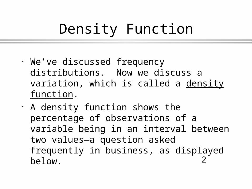
The Percentages
The total area under the curve is the percentage of observations that are greater than minus infinity but less than infinity. It is therefore 1 or 100%.
The percentage of observations that are less than x2 but larger than x1:
4
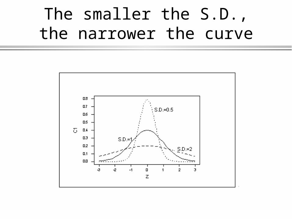
The smaller the S.D., the narrower the curve
5
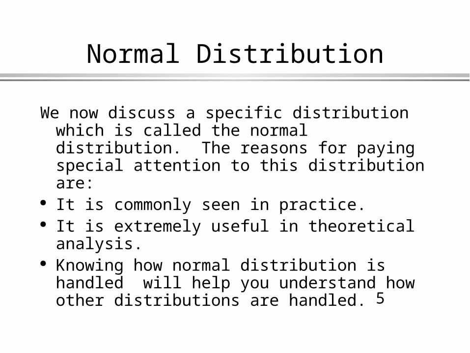
Normal Distribution
We now discuss a specific distribution which is called the normal distribution. The reasons for paying special attention to this distribution are:
It is commonly seen in practice. It is extremely useful in theoretical analysis. Knowing how normal distribution is handled
will help you understand how other distributions are handled.
6
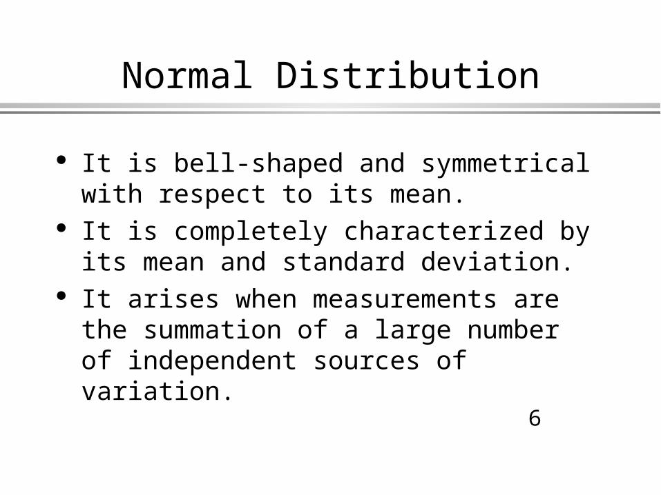
Normal Distribution
It is bell-shaped and symmetrical with respect to its mean.
It is completely characterized by its mean and standard deviation.
It arises when measurements are the summation of a large number of independent sources of variation.
7
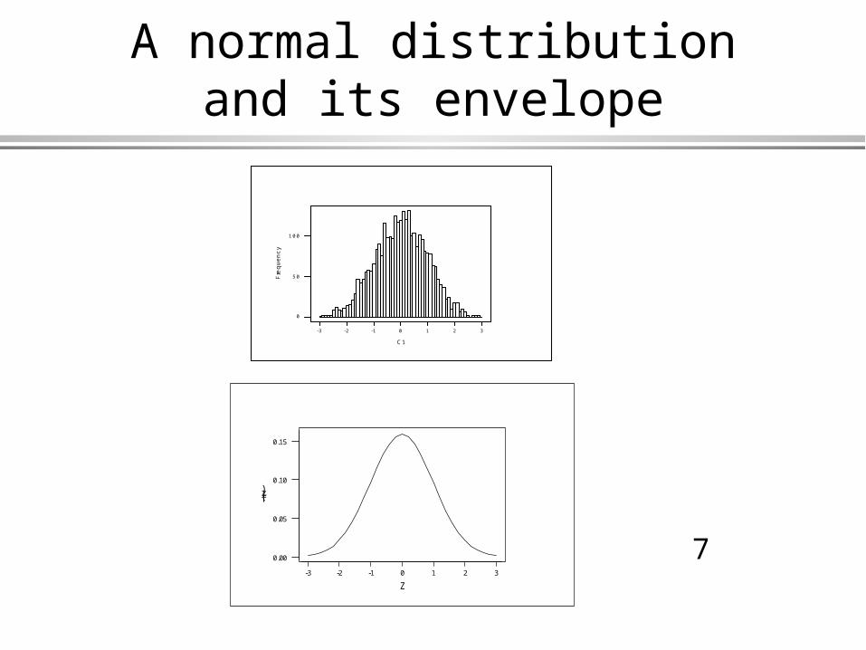
A normal distribution and its envelope
3210-1-2-3
100
50
0
C1
Freq
uenc
y
3210-1-2-3
0.15
0.10
0.05
0.00
Z
f(z)
8
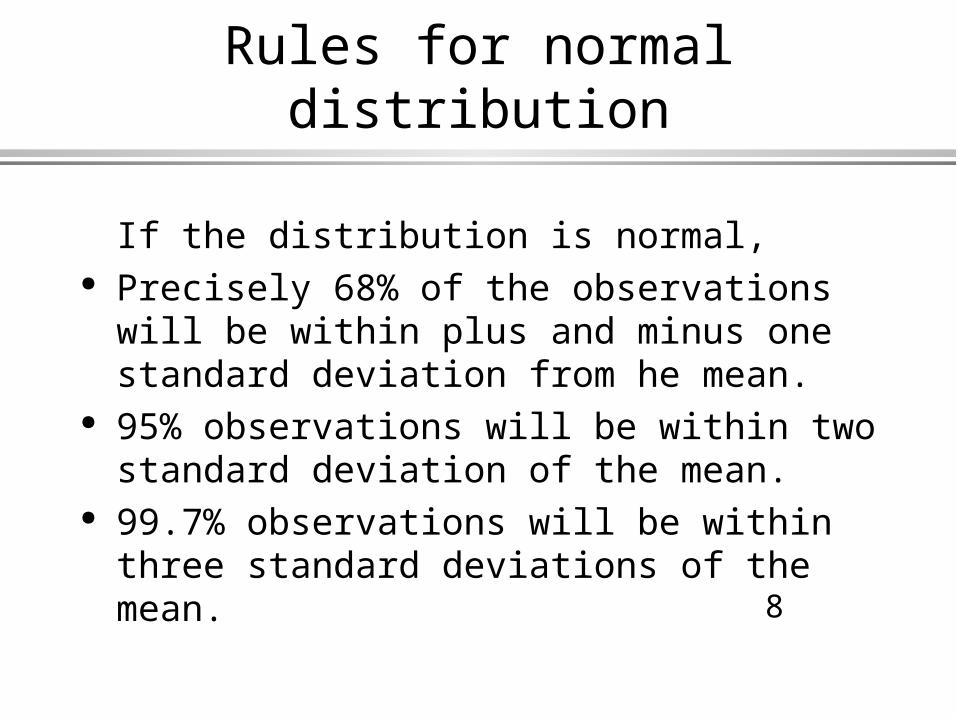
Rules for normal distribution
If the distribution is normal, Precisely 68% of the observations will be
within plus and minus one standard deviation from he mean.
95% observations will be within two standard deviation of the mean.
99.7% observations will be within three standard deviations of the mean.

9
Computing percentages
The less-than problem. We ask: what is the percentage of observations that are less than a specific value, say 2.0?
The greater-than problem. We ask: what is the percentage of observations that are greater than a specific value, say 1.5?
The in-between problem. We ask: what is the percentage of observations that are greater than a specific value, say 1.5, but less than another value, say 2.0?
10
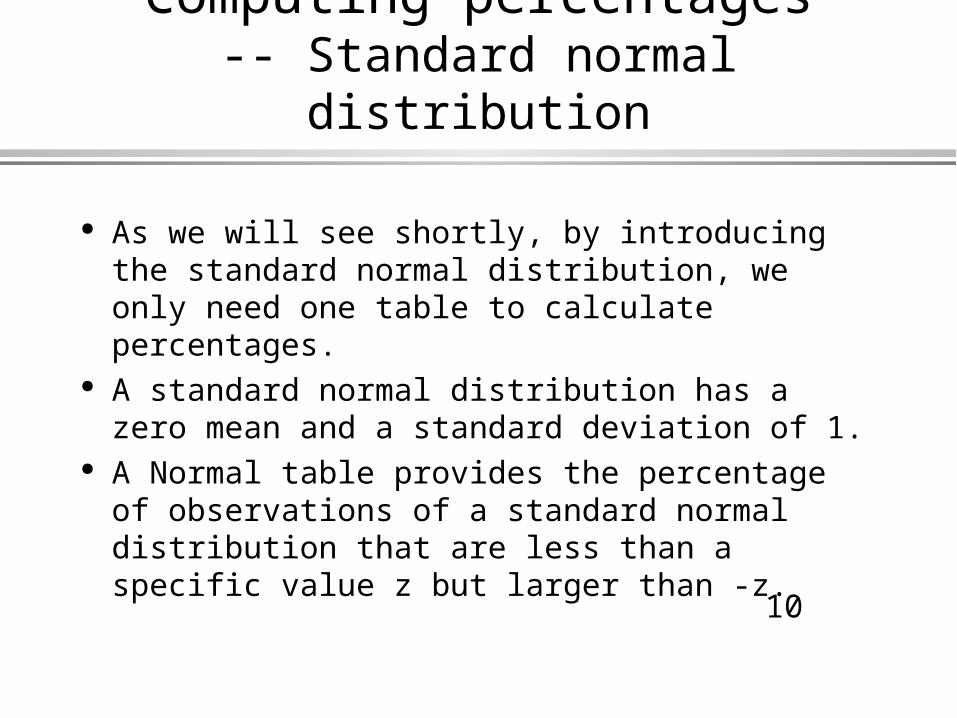
Computing percentages-- Standard normal distribution
As we will see shortly, by introducing the standard normal distribution, we only need one table to calculate percentages.
A standard normal distribution has a zero mean and a standard deviation of 1.
A Normal table provides the percentage of observations of a standard normal distribution that are less than a specific value z but larger than -z.

11
The Normal Table
The normal table shows the percentage of observations of a standard normal distribution that are less than a specific value z but larger than -z. Assume z=2. Graphically, we have
12
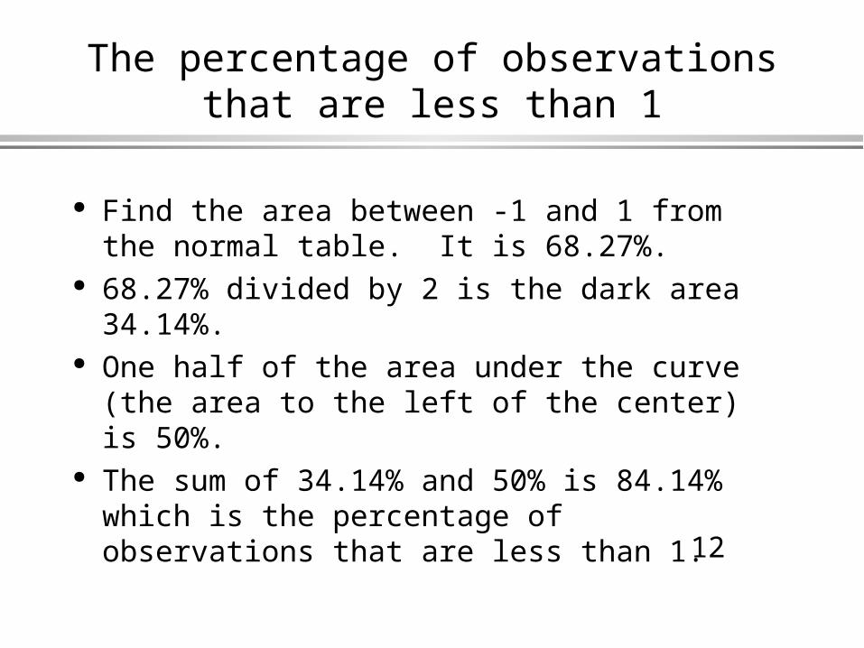
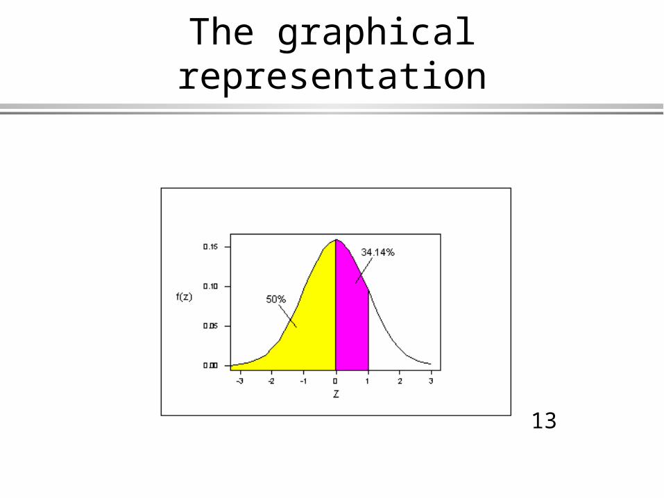
The percentage of observations that are less than 1
Find the area between -1 and 1 from the normal table. It is 68.27%.
68.27% divided by 2 is the dark area 34.14%. One half of the area under the curve (the
area to the left of the center) is 50%. The sum of 34.14% and 50% is 84.14%
which is the percentage of observations that are less than 1.
13
The graphical representation
14
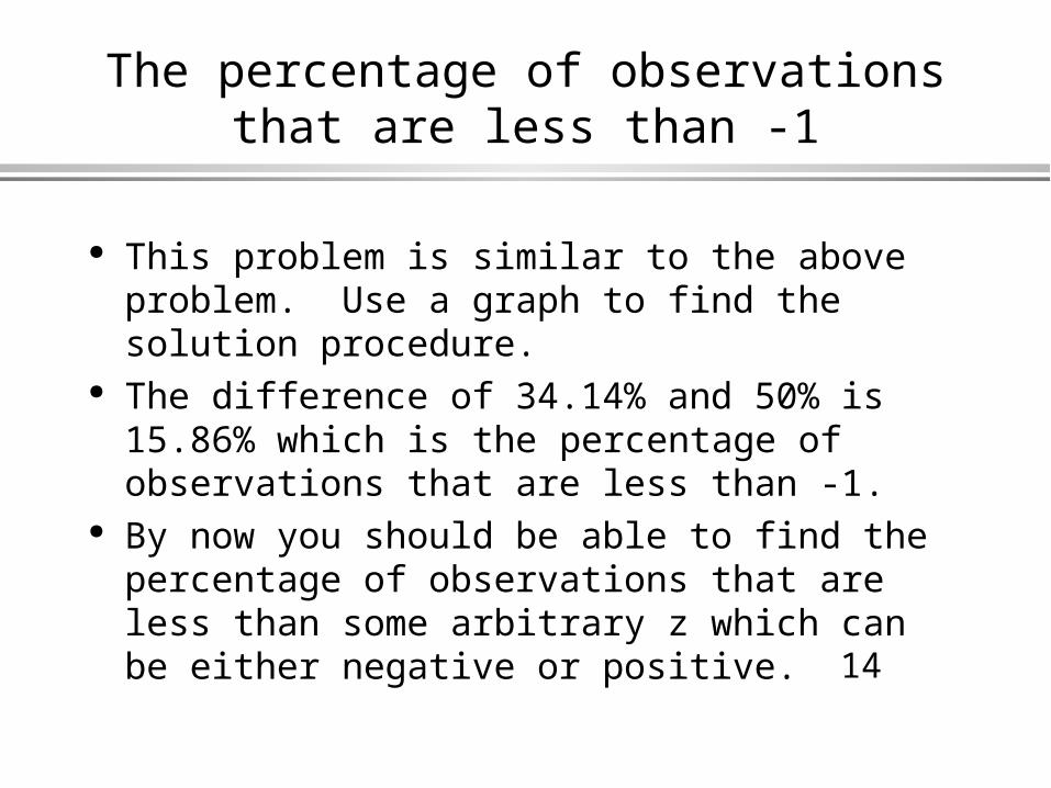
The percentage of observations that are less than -1
This problem is similar to the above problem. Use a graph to find the solution procedure.
The difference of 34.14% and 50% is 15.86% which is the percentage of observations that are less than -1.
By now you should be able to find the percentage of observations that are less than some arbitrary z which can be either negative or positive.

15
Other problems
A greater-than problem can be converted into a less-than problem. That is, the percentage of observations that are greater than 2 is equal to 100% minus the percentage of observations that are less than 2.
An in-between problem can be converted into two less-than problems.
16
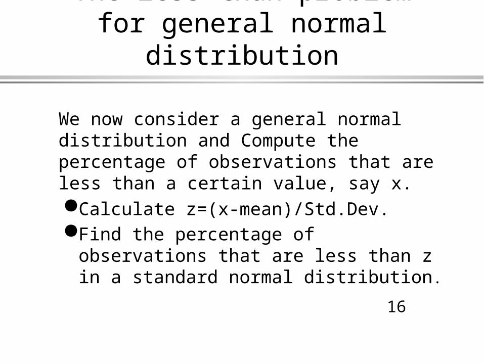
The less-than problem for general normal distribution
We now consider a general normal distribution and Compute the percentage of observations that are less than a certain value, say x.Calculate z=(x-mean)/Std.Dev.Find the percentage of observations that
are less than z in a standard normal distribution.

17
The greater-than problem
Calculating the percentage of observations that are greater than a certain value, say x.Solve a less-than problem first, i.e., find the
percentage of observations that are less than x. Assume the result is P.
The solution for the greater-than problem is 1-P.
18
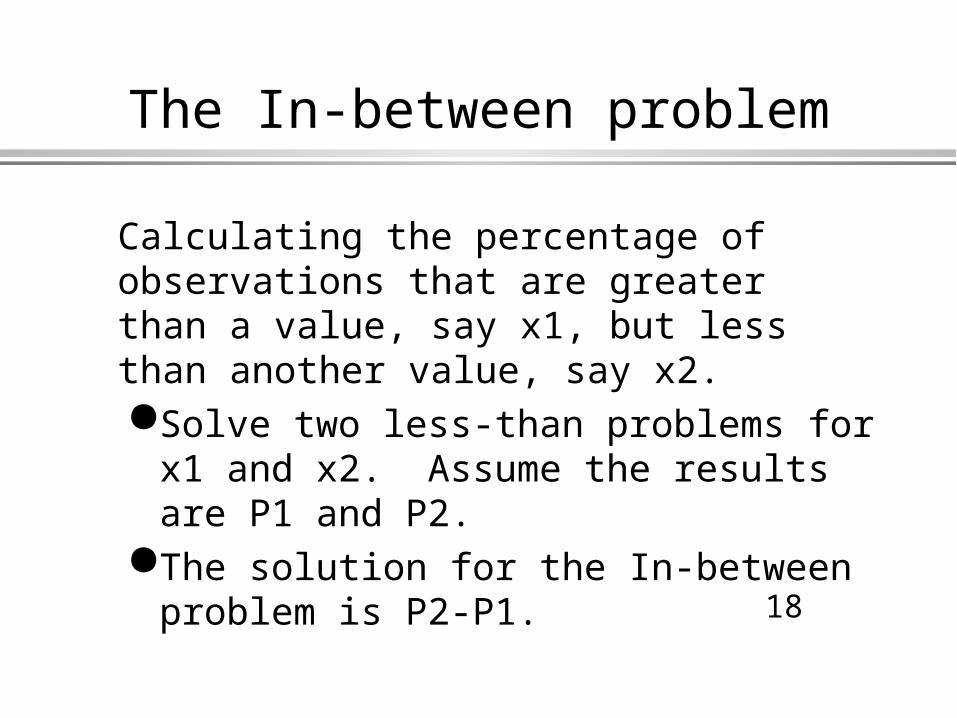
The In-between problem
Calculating the percentage of observations that are greater than a value, say x1, but less than another value, say x2.Solve two less-than problems for x1 and
x2. Assume the results are P1 and P2.The solution for the In-between problem is
P2-P1.
19
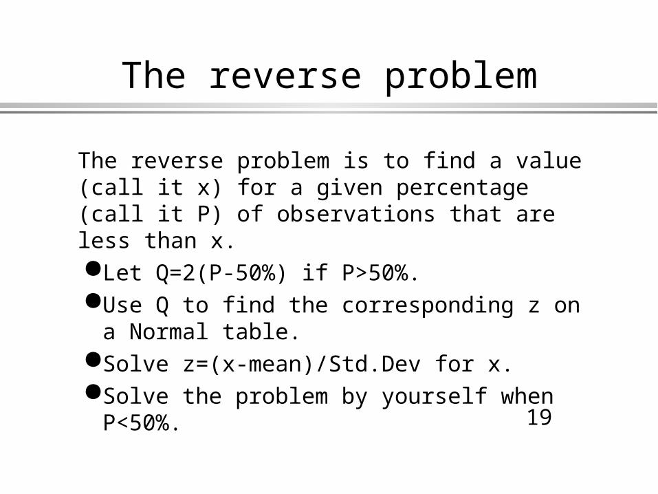
The reverse problem
The reverse problem is to find a value (call it x) for a given percentage (call it P) of observations that are less than x.Let Q=2(P-50%) if P>50%.Use Q to find the corresponding z on a
Normal table.Solve z=(x-mean)/Std.Dev for x.Solve the problem by yourself when
P<50%.
20
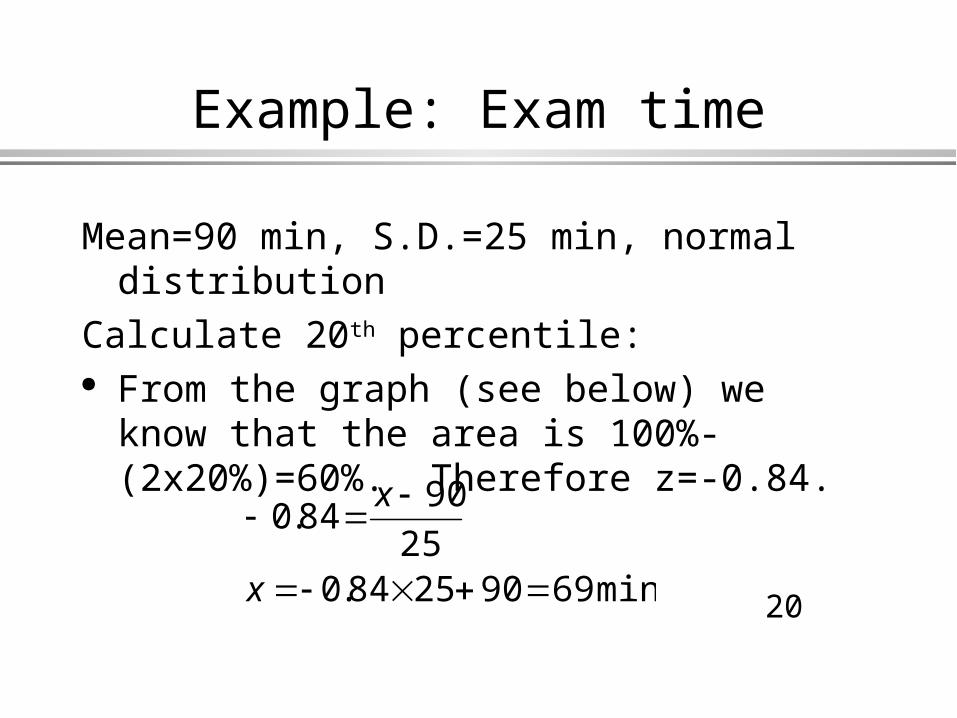
Example: Exam time
Mean=90 min, S.D.=25 min, normal distribution
Calculate 20th percentile: From the graph (see below) we know that the
area is 100%-(2x20%)=60%. Therefore z=-0.84.
min69902584.025
9084.0
x
x
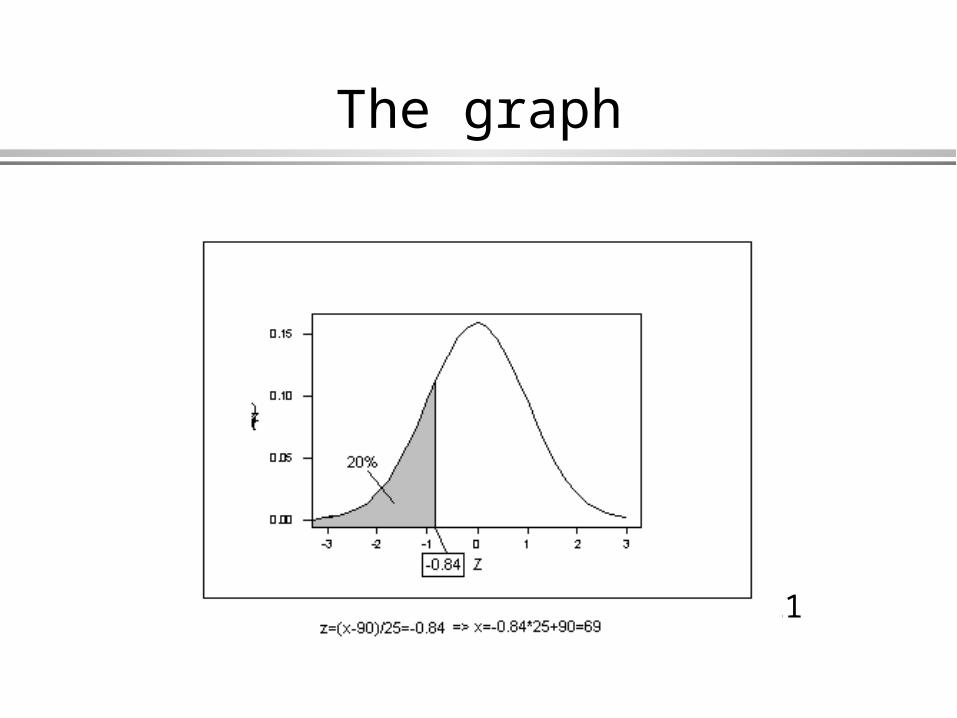
21
The graph
22
Verify Normal distribution
To see whether a distribution is normal or not:Store the data in a column, say C1.Use Minitab
Recommended