ANDREW YOUNG SCHOOL O F P O L I C Y S T U D I E S
Does Economic Prosperity Breed Trust?
Markus Brueckner, Alberto Chong and Mark Gradstein*
Abstract
We explore whether national economic prosperity enhances mutual generalized trust. This
is done using panel data of multiple waves of the World Values Surveys, whereby national
income levels are instrumented for using exogenous oil price shocks. We find significant
and substantial effects of national income on the level of trust in the economy. In particular,
a one percent increase in national income tends to cause an average increase of one
percentage point (or more) in the likelihood that a person becomes trustful. One possible
rationalization for this, exhibited in a simple model, is that perceived prosperity signals that
many people are trustworthy.
Keywords: Generalized trust; national income; oil price shocks
* Brueckner: Department of Economics, University of Queensland, Australia; Chong: Department of
Economics, Georgia State University, USA; Gradstein: Department of Economics, Ben Gurion University,
Israel. Acknowledgments to be added.

2
1. Introduction
Social capital and, in particular, the level of trust in an economy, has been shown to be
correlated with economic performance, specifically, with economic growth, see the seminal
work Knack and Keefer, 1997, Zak and Knack, 2001, and a survey Guiso et al., 2008, as well
as the more recent Algan and Cahuc, 2013, Bjornskov, 2012.1 While this has been mostly
exhibited in a cross national setting, Dincer and Uslaner, 2010, find positive associations
between trust and economic growth across the US states as well.
Generalized trust (i.e., trust in anonymous individuals, as opposed to trust among familiar
people) may positively affect welfare in a society through better cooperation, i.e. trust is
instrumental in avoiding prisoner dilemma outcomes. See Banfield, 1958, for a pioneering
work; effects of trust on various aggregate outcomes have been explored in, for example,
Aghion et al., 2010, Bjornskov, 2009, 2010, Bjornskov and Meon, 2013, Bjornskov and
Svendsen, 2013. The documented importance of trust implies that there is potential interest
in studying its nation-wide determinants. This has been done in, for example, Bjornskov,
2006, although identification obstacles in disentangling causality have been acknowledged
by the author.
One important question in this regard is whether economic prosperity and, in
particular, higher national income breeds trust. Indeed, already in Banfield, 1958, economic
backwardness and poverty are viewed not only as a consequence, but also as a cause of
distrust. While some positive indications on the causal effect of income on trust are provided
in Bjornskov, 2006, this question has received relatively little attention so far. The recent
1Fukuyama, 1995, and Uslaner, 2002, provide conceptual underpinnings for this relationship.

3
paper, Ananyev and Guriev, 2015, addresses it by focusing on a natural experiment, whereby
Russia’s administrative regions were differently affected by the aftermath of the 2008-9
economic crisis. In particular, whereas the average GDP decline in Russia was eight percent,
the per capita gross regional product declined more in Russian regions that specialized in the
production of capital-intensive goods. The heterogenous impact of the 2008-2009 economic
crisis across regional differences in industrial structures enables the authors to explore the
effect of regional variation in income on trust. They find that reductions in regional income
lead to a deterioration of trust. Their estimated effect is sizable: a ten percent decline in
income causes a 2.6 percentage points reduction in the level of trust.2
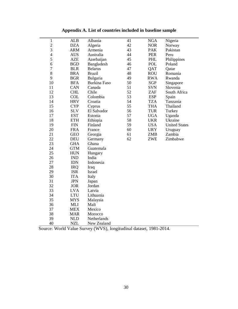
In this paper, our goal is to add to the literature by analyzing the effect of income on
trust in a broader context. We use a cross-country panel data set comprising 62 countries
during the period 1981-2010. Our data on trust are from the World Values Survey. These
data have been used widely in the literature (see, for example, Guiso et al., 2008) to explore
the relationship between trust and other variables, including economic growth. We
contribute to this literature in several ways. First, we extend extant analysis by including
more recent survey waves – which incidentally provide ever more comprehensive country
coverage. Second, by including country fixed effects we focus on within-country variations
in national income and trust, thus controlling for all the potentially omitted fixed factors.
Third, we use oil price shocks as an instrumental variable for national income, which enables
us to extract exogenous variation in national economic prosperity. The oil price shock
instrument for national income has been used in the literature in several contexts (e.g.,
2 This broad conclusion is also confirmed in the extended context of transition economies in Ananyev and
Guriev, 2015.

4
Brueckner et al., 2012a, b), and it has been found to be a strong IV for persistent variation in
national income.
We, therefore, relate individual trust attitudes to nation-wide exogenous income, at
the same time controlling for a battery of individual specific characteristics. We find that
national income has a significant effect on trust attitudes. In particular, a one percent increase
in national income tends to cause an average increase of one percentage point in the
likelihood that a person becomes trustful. While this is generally consistent with existing
studies, the contribution here is in interpreting the result in causal terms. Our approach and
results are broadly consistent with Ananyev and Guriev, 2015; while that paper does not use
oil price shocks to generate variation in income, the spirit of its analysis is similar.
We construct a simple model to rationalize our finding. In the model, productivity
hinges upon the perceived share of trustworthy individuals. Income growth enables the
individuals to infer that this share is high, whereas the opposite holds in the case of
stagnation. This establishes the existence of a causal effect of national income growth on the
level of trust in the economy.
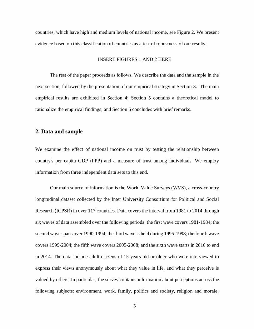
To motivate our research we present graphical evidence of the relationship between
per capita GDP and average trust that is prevalent in countries. As observed in Figure 1 there
is a positive and significant correlation between these two variables in our sample. This
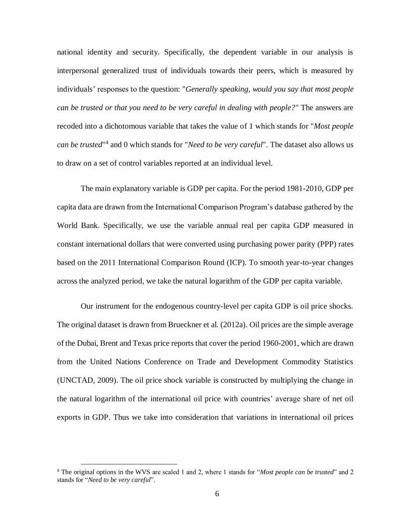
pattern is also present when distinguishing between OECD member3 and non-member
3 These are Australia, Canada, Chile, Estonia, Ethiopia, Finland, France, Germany, Hungary, Israel, Italy, Japan,
Mexico, Netherlands, Norway, Poland, Spain, Turkey, United States.
5
countries, which have high and medium levels of national income, see Figure 2. We present
evidence based on this classification of countries as a test of robustness of our results.
INSERT FIGURES 1 AND 2 HERE
The rest of the paper proceeds as follows. We describe the data and the sample in the
next section, followed by the presentation of our empirical strategy in Section 3. The main
empirical results are exhibited in Section 4; Section 5 contains a theoretical model to
rationalize the empirical findings; and Section 6 concludes with brief remarks.
2. Data and sample
We examine the effect of national income on trust by testing the relationship between
country's per capita GDP (PPP) and a measure of trust among individuals. We employ
information from three independent data sets to this end.
Our main source of information is the World Value Surveys (WVS), a cross-country
longitudinal dataset collected by the Inter University Consortium for Political and Social
Research (ICPSR) in over 117 countries. Data covers the interval from 1981 to 2014 through
six waves of data assembled over the following periods: the first wave covers 1981-1984; the
second wave spans over 1990-1994; the third wave is held during 1995-1998; the fourth wave
covers 1999-2004; the fifth wave covers 2005-2008; and the sixth wave starts in 2010 to end
in 2014. The data include adult citizens of 15 years old or older who were interviewed to
express their views anonymously about what they value in life, and what they perceive is
valued by others. In particular, the survey contains information about perceptions across the
following subjects: environment, work, family, politics and society, religion and morale,
6
national identity and security. Specifically, the dependent variable in our analysis is
interpersonal generalized trust of individuals towards their peers, which is measured by
individuals’ responses to the question: "Generally speaking, would you say that most people
can be trusted or that you need to be very careful in dealing with people?" The answers are
recoded into a dichotomous variable that takes the value of 1 which stands for "Most people
can be trusted"4 and 0 which stands for "Need to be very careful". The dataset also allows us
to draw on a set of control variables reported at an individual level.
The main explanatory variable is GDP per capita. For the period 1981-2010, GDP per
capita data are drawn from the International Comparison Program’s database gathered by the
World Bank. Specifically, we use the variable annual real per capita GDP measured in
constant international dollars that were converted using purchasing power parity (PPP) rates
based on the 2011 International Comparison Round (ICP). To smooth year-to-year changes
across the analyzed period, we take the natural logarithm of the GDP per capita variable.
Our instrument for the endogenous country-level per capita GDP is oil price shocks.
The original dataset is drawn from Brueckner et al. (2012a). Oil prices are the simple average
of the Dubai, Brent and Texas price reports that cover the period 1960-2001, which are drawn
from the United Nations Conference on Trade and Development Commodity Statistics
(UNCTAD, 2009). The oil price shock variable is constructed by multiplying the change in
the natural logarithm of the international oil price with countries’ average share of net oil
exports in GDP. Thus we take into consideration that variations in international oil prices
4 The original options in the WVS are scaled 1 and 2, where 1 stands for “Most people can be trusted” and 2
stands for “Need to be very careful”.
7
affect countries national incomes depending on their commercial position as net importers or
exporters. Formally, the oil price shock instrument is constructed as follows:
𝑂𝑖𝑙𝑃𝑟𝑖𝑐𝑒𝑆ℎ𝑜𝑐𝑘𝑐,𝑡 = ∆In(𝑂𝑖𝑙𝑃𝑟𝑖𝑐𝑒)𝑡 ∗ 𝜃𝑐 (1)
where, ∆In(𝑂𝑖𝑙𝑃𝑟𝑖𝑐𝑒)𝑡 is the difference in the natural log of the international oil price in
period 𝑡 in comparison to the previous year; and weights it by the average share of net oil
exports over GDP. This is denoted by the time-invariant factor 𝜃𝑐 that corresponds to country
𝑐5. For the estimation sample, summary statistics of the oil price shock variable for period 𝑡
are reported in Table 1.
INSERT TABLE 1 HERE
For the purpose of this study, we consolidate the information from the three sources
described above. The resulting core sample comprises 164,457 individual-level observations
for 62 countries; this sample is dictated by the available data on trust, income, and the oil
price shock instrument. The list of home countries of the analyzed individuals is presented
in Appendix A. Also, the full set of variables tested to control individual and country’s
characteristics are reported with summary statistics in Table 1. We present specifications
including main basic controls such as gender, age, marital status, number of children, and
highest education level achieved. The definition of these variables is explained in detail in
Appendix B. Finally, the summary statistics of the proposed instrument in the estimation
sample is also reported in Table 1.
5 The values of 𝜃𝑐 range from -0.03 to 0.18, with a mean of 0.009 (see details in Brueckner et al. 2012a).
8
3. Empirical framework
Baseline specification
Our goal is to estimate the effect of national income on interpersonal trust. The literature, see
the survey section in the introduction, has addressed this topic empirically both at the country
and at the individual level; and it has shown that higher-income individuals have indeed
higher levels of trust. Nevertheless, empirical papers thus far have mainly drawn conclusions
based on correlations between the studied variables, leaving open the question whether trust
increments nationwide are caused by higher income levels.
We attempt to quantify the causal effect of national income on trust among
individuals based on cross country analysis, using log per capita GDP that accounts for the
average individual’s income; and a broad trust measure in the sense that it doesn’t capture
confidence with respect to a specific group (e.g. by ethnicity, organizations, institutions). For
this purpose, we employ an estimation strategy set at the individual level. Our baseline
econometric model is given by:
𝑇𝑟𝑢𝑠𝑡𝑖𝑗𝑡 = 𝛼 + 𝛾𝑙𝑛(𝑝𝑒𝑟 𝑐𝑎𝑝𝑖𝑡𝑎 𝐺𝐷𝑃 𝑃𝑃𝑃𝑗𝑡) + 𝑋𝑖𝑗𝑡′ 𝛿 + 𝜑𝑡 + 𝜏𝑗 + 휀𝑖𝑗𝑡 (2)
where 𝑇𝑟𝑢𝑠𝑡𝑖𝑗 is the reported trust level of individual 𝑖 in country 𝑗 in period 𝑡 that
corresponds to the year when the survey was conducted. 𝑃𝑒𝑟 𝑐𝑎𝑝𝑖𝑡𝑎 𝐺𝐷𝑃 𝑃𝑃𝑃𝑗 corresponds
to average income at purchasing power parity of country 𝑗 for the corresponding period in
which the individual reports her or his level of trust. Thus 𝛾 is our parameter of interest,
which measures the response of trust to a change in national income.

9
We include in the econometric model time and country fixed effects, and individual level
controls to increase the efficiency of our parameter estimates. We compute standard errors
that are Huber robust and clustered at the country level.
Identification
We consider that least squares estimation of equation (2) does not provide consistent
estimates of 𝛾 since, in particular, trust affects income per capita. To address causality issues
we use plausibly exogenous oil price shocks as an instrument of log per capita GDP, within
a conditional joint maximum likelihood estimation method allowing for national income to
be endogenous.
Our identification assumption is that the oil price shock instrument only has a
systematic effect on trust through variations in national income. Moreover, we propose that
lagged values of oil price shocks are likely to affect per capita GDP as do contemporary
shocks due to its persistent effect. In particular, the second-stage equation is given by:
𝑇𝑟𝑢𝑠𝑡𝑖𝑗𝑡 = 𝛽𝐸[𝑙𝑛(𝑝𝑒𝑟 𝑐𝑎𝑝𝑖𝑡𝑎 𝐺𝐷𝑃𝑗𝑡)|�̅�𝑗𝑡] + �̅�𝑖𝑗𝑡′ 𝛿 + 𝜑𝑡 + 𝜏𝑗 + 휀𝑖𝑗𝑡 (3)
where 𝑇𝑟𝑢𝑠𝑡𝑖𝑗𝑡 is the trust indicator of individual 𝑖 that lives in country 𝑗 in period 𝑡. We
control for a set of individual characteristics expressed in vector �̅�𝑖𝑗𝑡 and country-specific
fixed effects (𝜏𝑗) to account for within-country factors that affect both trust and income levels.
We also allow survey year fixed effects (𝜑𝑡) in our specification. The term
𝐸[𝑙𝑛(𝑝𝑒𝑟 𝑐𝑎𝑝𝑖𝑡𝑎 𝐺𝐷𝑃)𝑖𝑗𝑡|�̅�𝑖𝑗𝑡] stands for the predicted level of log per capita GDP obtained
from �̅�𝑖𝑗𝑡, which is a vector of variables including 𝑍𝑗𝑡 , 𝑍𝑗𝑡−1 and 𝑍𝑗𝑡−2. In particular, the
predicted level of log per capita GDP is obtained from the following equation:
10
𝑙𝑛(𝑝𝑒𝑟 𝑐𝑎𝑝𝑖𝑡𝑎 𝐺𝐷𝑃𝑖𝑗𝑡) = 𝜋0𝑍𝑗𝑡 + 𝜋1𝑍𝑗𝑡−1 + 𝜋2𝑍𝑗𝑡−2 + 𝑋𝑖𝑗𝑡′ 𝜃 + 𝜔𝑗 + 𝜏𝑡 + 𝜃𝑗𝑡 + 𝜇𝑖𝑗𝑡 (4)
Equation (4) corresponds to our first stage equation. The set of variables Zjt , Zjt−1
and Zjt−2 correspond to the instruments, i.e. one contemporaneous (for period 𝑡) and two
lagged values of oil price shocks (for periods 𝑡-1 and t-2). Various specifications of lagged
values were tested to capture the persistent income effects triggered by variations in the oil
price instrument. Specifically, the IV employed are the following: (1) contemporaneous oil
price shock; (2) oil price shock of period t-1; (3) oil price shock of period t-2; (4) oil price
shock of period t and t-1; and (5) oil price shocks of periods t, t-1 and t-2. As documented in
Brueckner et al. (2012a, 2012b), there is a strong correlation between the vector �̅�𝑖𝑗𝑡 and
𝑙𝑛(𝑝𝑒𝑟 𝑐𝑎𝑝𝑖𝑡𝑎 𝐺𝐷𝑃𝑖𝑗𝑡), implying 𝜋0 ≠ 0, 𝜋1 ≠ 0, 𝜋2 ≠ 0.
4. Results
In Table 2 we present baseline estimates of the effects of country's per capita GDP on trust
in people. The estimates are based on the model described in the previous section. We report
three specifications in which country and survey years’ fixed effects are included. Column
(1) examines the unconditional effect of real per capita income on a general measure of trust
in people. Column (2) shows this effect when controlling in the econometric model for a set
of potentially relevant individual characteristics; and column (3) adds the highest educational
level attained as a trust determinant.
Columns (1)-(3) of Table 2 show a statistically significant and positive income effect on trust.
Quantitatively, we observe that this relationship is stronger when controlling for differences
in individuals’ education.

11
INSERT TABLE 2 HERE
In order to obtain an estimate of the causal effect of national income on individuals’
trust we use an IV approach. Maximum likelihood estimates of how (instrumented) national
real per capita GDP affect the levels of average trust attitudes towards people are reported in
Table 3. We begin by exploring this effect using oil price shocks of period t as instrument
for real per capita income reported during period t. Both country and survey year’s fixed
effects are included in the regression. Columns (1) to (3) of Table 3 show that a positive
effect of national income on trust holds across the three specifications thus far described.
Instrumental variables estimation yields a positive effect of national income on trust.
We can reject the null that the coefficient on national income is equal to zero at the 1 percent
significance level for all three specifications. Quantitatively, the coefficient on national
income is largest in column (3) where we control for individuals’ characteristics, in
particular, education. The coefficient (standard error) on national income in column (3) is
around 1.46 (0.29). This coefficient should be interpreted as a one percent increase in GDP
per capita increasing the likelihood of trust by around 1.46 percentage points. Roughly, the
IV estimate in table 3 can thus be read as a one percent increase in national income increasing
the likelihood of trust by 1 percentage point.
INSERT TABLE 3 HERE
It is noteworthy that the instrumental variables regressions in Table 3 yield
coefficients on national income that are larger than those reported in Table 2 (where national
income is not instrumented). For each specification, we can reject the null hypothesis that the
coefficient in Table 3 is equal to the coefficient in Table 2 at the 1 percent significance level.

12
Hence, not instrumenting GDP per capita leads to an understatement of the causal effect that
national income has on trust.
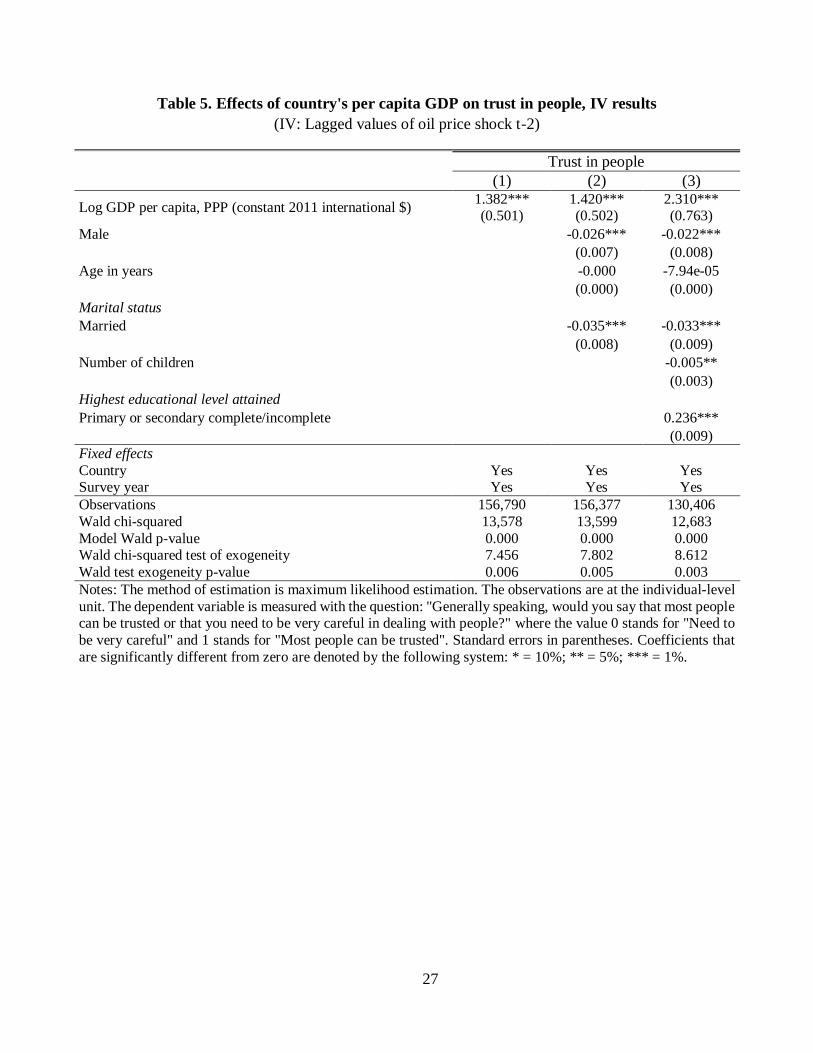
Tables 4 and 5 document that the second-stage coefficients on national income are of
similar magnitude and statistical significance when we use lagged oil price shocks of periods
t-1 and t-2 as instruments for per capita GDP of period t.
INSERT TABLES 4 TO 5 HERE
Since the effect of oil shocks on GDP per capita may remain for periods longer than
a year, a longer period set of lagged oil price shocks are also considered as instruments. Oil
price shocks for period t and t-1 are used as instruments in Table 6. Here, we find a positive
and significant link between per capita GDP and trust.
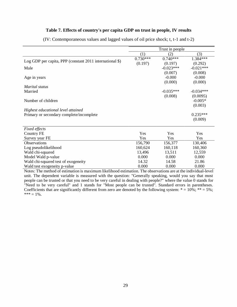
Using a more comprehensive set of instruments supports our main finding that income
has a significant positive effect on trust. Table 7 includes contemporaneous (period t) and
lagged oil price shocks in period t-1 and t-2 as instruments. As can be seen from Table 7, the
coefficients on national income continue to be positive and significantly different from zero
at the 1 percent significance level. Quantitatively, the second-stage coefficient on national
income is around unity. We note that the quality of our instrumental variables is reasonable
as the p-value of the F-statistic is below 1%; further the F-statistic is well above 10.
INSERT TABLES 6 TO 7 HERE
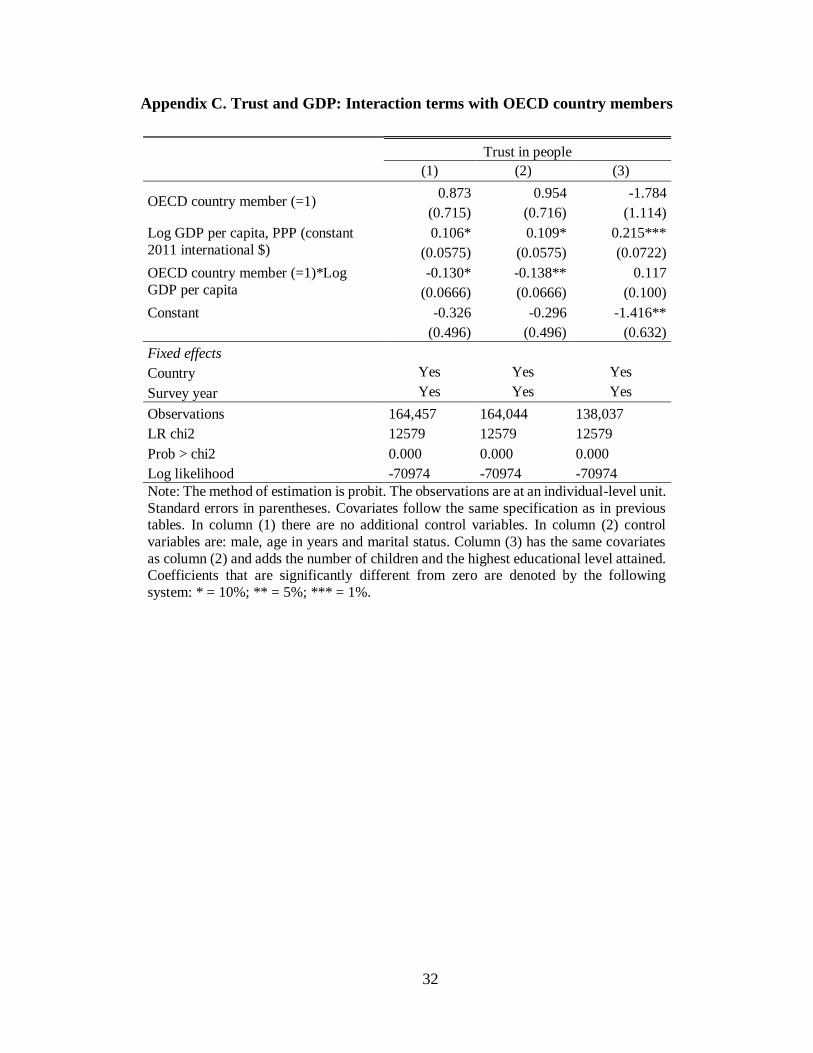
In addition to the results presented above, we also test for heterogeneous effects by
introducing an interaction term between GDP and membership in the OECD. The purpose of
this is to examine whether the impact of GDP is different in richer countries in relation to

13
poorer ones. In Appendix C we observe that whereas the GDP coefficient remains
statistically significant for all specifications, the coefficient on the interaction term is negative
and statistically significant for the first two specifications only, and is insignificant when
adding controls, as shown in the third column. Furthermore, when using our instrumental
variables approach we find statistically insignificant results for all our specifications6. These
additional results show limited evidence that the impact of national income on trust differs
systematically for OECD countries
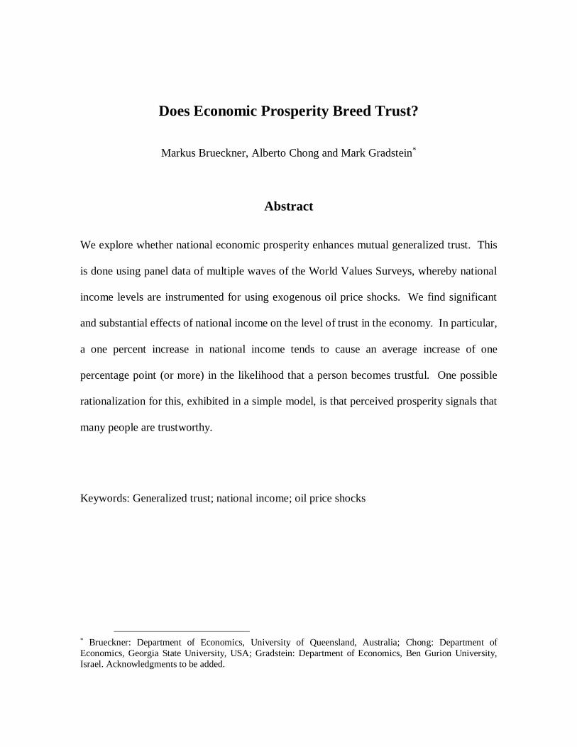
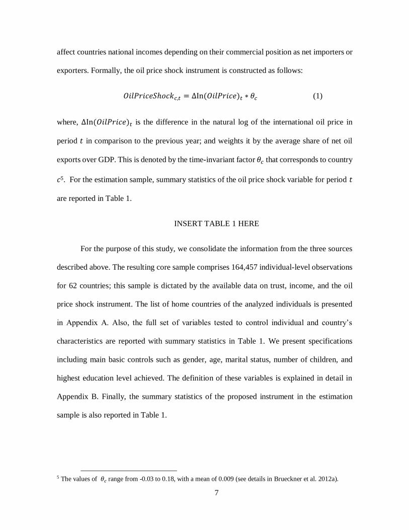
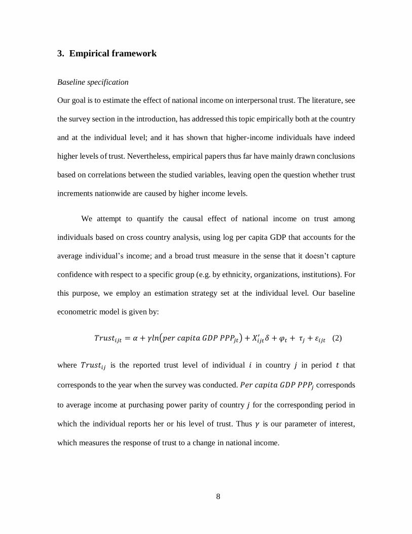
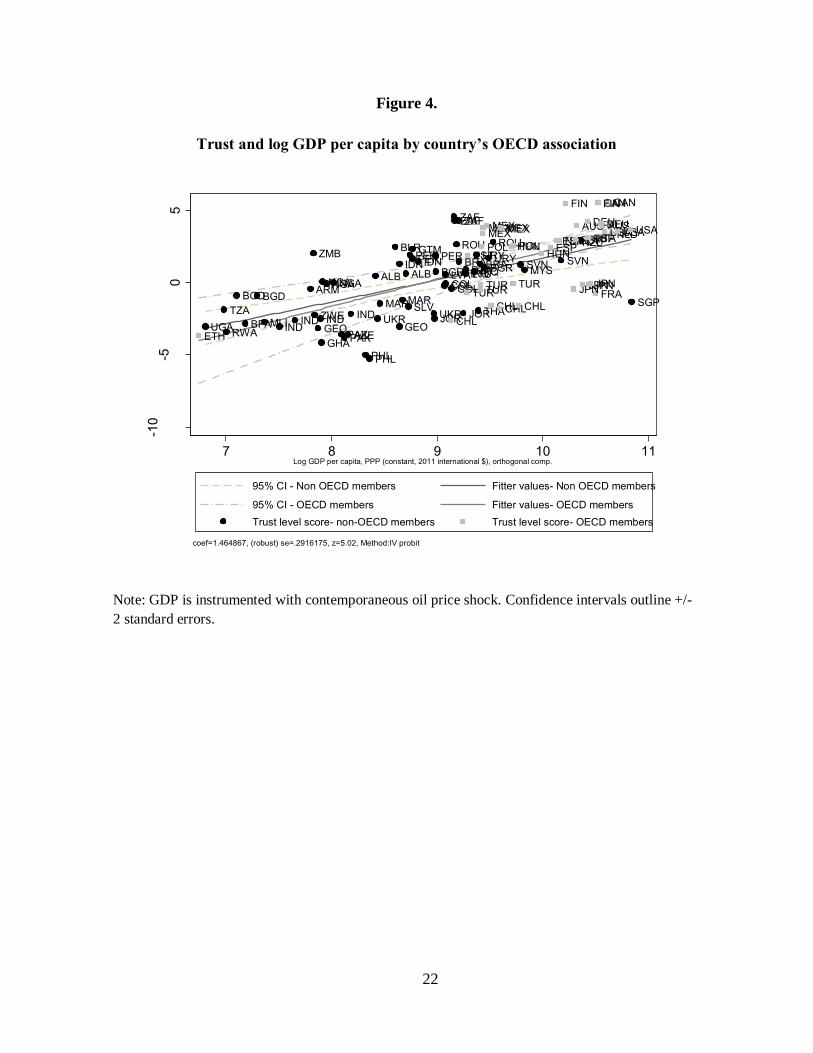
We summarize our findings graphically in Figures 3 and 4. In these figures variations
in GDP are induced by the oil price shock instrument. In the first figure we see a significant
positive average relationship between per capita GDP and trust. The slope of the fitted line
in Figure 3 is steeper than in Figure 1. Thus, the magnitude of the effect of national income
on trust is stronger when instrumenting GDP by plausibly exogenous oil price shocks. Figure
4 shows the estimated slopes for OECD and non-OECD countries. We observe that the slope
is somewhat higher for OECD than non-OECD countries although quantitatively this
difference is minuscule and the 95 percent confidence bands overlap.
INSERT FIGURES 3 AND 4 HERE
5. A model
We present a stylized model in order to illustrate a possible mechanism through which the
detected effect of national income on trust can materialize.
6 The instrumental variables results are not reported here.
14
The framework
Consider an economy populated by identical households, indexed i, each consisting of a
parent and a child, with a unit measure, that operates over discrete time periods t. We let yt
denote each household’s period t’s income; ct – its consumption; and kt+1 its capital
investment. The initial income level, y0, is given. A household’s budget constraint is:
(5) yt = ct + kt+1
Income production function is given as follows:
(6) yt = Atkt
where At > 0 is TFP, which is assumed to depend on the level of trust in the economy.
Specifically, we assume that At = 1+st, where st is the share of trustworthy individuals. There
is uncertainty in regard to this share, which is assumed to be distributed, in each period,
binomially, i.e., st=1 with the probability t and st=0 with the probability 1-t; t is interpreted
as the level of trust in the economy. We let Et denote the expected value of the probability
of st=1, t. Initially, 0 is distributed according to a known distribution in the interval [0,1],
and the distribution of individuals’ subsequent trust beliefs evolves over time.
Parents derive utilities from family consumption and their offspring’s income, U(ct,
yt+1); to simplify matters we impose the following functional form:
(7) U(ct, yt+1) = ln(ct) + yt+1
In each period, parents allocate family income, subject to the budget constraints, so
as to maximize the expected utility with respect to the share of honest individuals. And they,
further, update their trust priors, upon observing income realizations. In equilibrium, all these
decisions are mutually consistent.

15
Analysis
In any period t, the first order condition with respect to the investment amount is:
(8) -1/(yt - kt+1) + 1+Et+1 = 0,
so that
(9) kt+1 = yt – 1/(1+ Et+1)
The substitution of which into the production function yields:
(10) yt+1 = (1+st+1)(yt – 1/(1+ Et+1))
It then follows, since st+1 is a Bernoulli variable, that the prior distribution of yt+1 is
also Bernoulli. And both variables’ posterior follows from Bayesian updating. As the beta
distribution is a conjugate prior for Bernoulli, it is convenient to assume that 0 is distributed
according to the beta distribution, with parameters (0, 0), implying its expected value of
0/(0+0). Its expected value in subsequent periods can then be found recursively as
follows:
(11) Et+1 = (t + st+1)/(t+t+1), so that Et+1 > Et if st+1=1, and Et+1 < Et if st+1=0.
Whereas higher expected value of t+1 – hence, of TFP – positively affects investment,
it is also true that, because of the Bayesian updating, a higher value of observed income
implies an upward revision of the probability of being honest, hence, trust.
We, therefore, have the following implication of the model:
Proposition 1. A higher realization of national income leads to a higher level of trust in the
economy.

16
A higher level of national income induces individuals to infer that the share of trustworthy
individuals – hence, productivity – is high. Such Bayesian revision directly implies the
indicated causal relationship. The model is, therefore, consistent both with the established
result that trust affects growth prospects and with the presented finding that high national
income induces trust. Its dynamic extension – not pursued here - could indicate the
possibility of a mutual feedback between income and trust. It would lead to trust persistence,
which was found to be the case in some recent work, see Becker et al., 2014.
6. Concluding remarks
As generalized trust has been recognized an important factor for economic development, its
determinants deserve studying. Already Banfield, 1958, in his seminal study of distrust in
southern Italy advanced the hypothesis that poverty and backwardness can be one of the
determinants of distrust among people. Yet, more detailed evidence on this channel has been
sparse. In this paper, we use all available waves of the World Values Surveys to address the
issue. Employing an instrumental variable approach to overcome endogeneity biases and
focusing on within country variations, we find that national income has a positive effect on
the level of trust. In particular, an increase of one percent in the former variable leads to a
one percentage point increase in the likelihood of trust. This result is generally consistent
with the cross country study of Bjornskov, 2006, and with the study of Russia by Ananyev
and Guriev, 2015.

17
References
Aghion, P., Algan, Y., Cahuc, P., and A. Shleifer, 2010, “Regulation and Distrust,”
Quarterly Journal of Economics, 125, 1015-49.
Algan, Y. and P. Cahuc, 2013, “Trust, Growth and Well-being: New Evidence and Policy
Implications,” IZA DP No. 7464.
Ananyev M. and Guriev S., 2015, “Effect of Income on Trust: Evidence from the 2009
Crisis in Russia,” Sciences Po Economics DP.
Banfield, E.C., 1958, “The moral basis of a backward society”, Glencoe, Il, The Free Press.
Becker, S.O., K. Boeckh, C. Hainz, L. Woessmann, 2014, “The Empire Is Dead, Long
Live the Empire! Long-Run Persistence of Trust and Corruption in the Bureaucracy,”
Economic Journal, forthcoming.
Bjørnskov, Christian; Svendsen, Gert Tinggaard, 2013, “Does social trust determine the
size of the welfare state? Evidence using historical identification“ Public Choice, 157, 269-
286.
Bjørnskov, C., 2006, “Determinants of generalized trust: a cross-country comparison,”
Public Choice, 130, 1-21.
Bjørnskov, C., 2009, “Social trust and the growth of schooling”. Economics of Education
Review, 28, 249-257.
Bjørnskov, C., 2010, “How does social trust lead to better governance? An attempt to
separate electoral and bureaucratic mechanisms”. Public Choice, 144, 323-346.
Bjørnskov, C., 2012, “How does social trust lead to economic growth?” Southern Economic
Journal, 78, 1346-1368.
Bjørnskov, C. and Méon, Pierre-Guillaume, 2013, “Is Trust the Missing Root of
Institutions, Education, and Development?” Public Choice, 157, 641-669.
Brueckner, Markus, Antonio Ciccone, and Andrea Tesei. "Oil price shocks, income, and
democracy." Review of Economics and Statistics 94 (2012a): 389-399.
Brueckner, Markus, Alberto Chong, and Mark Gradstein. "Estimating the permanent
income elasticity of government expenditures: Evidence on Wagner's law based on oil price
shocks." Journal of Public Economics 96 (2012b): 1025-1035.
Dincer, O. and E. Uslaner, 2010, "Trust and Growth," Public Choice, 142, 59-67.

18
Fukuyama, F., 1995, “Trust: the social virtues and the creation of prosperity”. New York:
Free Press.
Guiso, L., Sapienza, P. and Zingales, L., 2008, Social capital as good culture. Journal of
the European Economic Association, 6, 295-320.
Knack, S. and Keefer, P., 1997, “Does social capital have an economic pay-off? A cross-
country investigation”. Quarterly Journal of Economics, 112, 1251-1288.
United Nations Conference on Trade and Development. 2009. “Commodity Price Series.
Online Database”.
Uslaner, E.M. 2002. “The moral foundations of trust”. Cambridge, UK: Cambridge
University Press.
Wooldridge, J. M., 2010., “Econometric analysis of cross section and panel data”. MIT
press.
Zak, P.J. and Knack, S., 2001, “Trust and growth,” The Economic Journal, 111, 295-321.

19
Figure 1.
Trust and log GDP per capita
Note: Correlation controlled for individual characteristics.
ALB ALB
DZA
ARM
AUS AUS
AZE
BGDBGD
BLR BRABRA
BGR BGR
BFA
CANCAN
CHL
CHLCHL
CHL
COLCOLCOL
CYP
SLV
EST
ETH
FIN FIN
FRA
GEO GEO
DEUDEU
GHA
GTMHUN
HUN
INDINDIND
IND
IDN
IDN
IRQIRQ
ITA
JPNJPNJPNJPN
JOR
JOR
LVALTUMYSMLI
MEXMEXMEX
MEXMEX
MAR
MAR
NLDNZL
NZLNGA
NGANGA
PAK
PAK
PER
PER
PER
PHL
PHL
POL POL
ROU ROU
RWA
SGP
SVNSVN
ZAFZAF
ZAF
ESPESPESP
ESP
TZA
THA
TURTUR
TUR
TUR
UGAUKR UKR
USAUSA
USA
URYURY
ZMB
ZWE
-2-1
01
2
Tru
st
leve
l score
(co
un
try a
ve
rag
e,
ort
ho
gon
al co
mp
.)
7 8 9 10 11Log GDP per capita, PPP (constant, 2011 international $), orthogonal comp.
Trust level score (average) Fitted values
coef=.19300663, (robust) se=0.070, z=5.02, Method: probit

20
Figure 2.
Trust and log GDP per capita by country’s OECD association
Note: Correlation controlled for individual characteristics.
ALB ALB
DZA
ARM
AZE
BGDBGD
BLR BRABRA
BGR BGR
BFA
COLCOLCOL
CYP
SLV
GEO GEO
GHA
GTM
INDINDIND
IND
IDN
IDN
IRQIRQ
JOR
JOR
LVALTUMYSMLI
MAR
MAR
NGANGANGA
PAK
PAK
PER
PER
PER
PHL
PHL
ROU ROU
RWA
SGPSVN
SVN
ZAFZAF
ZAF
TZA
THA
UGAUKR UKR
URYURY
ZMB
ZWE
AUS AUS
CANCAN
CHL
CHLCHL
CHL
EST
ETH
FIN FIN
FRA
DEUDEUHUNHUN
ITA
JPNJPNJPNJPN
MEXMEXMEX
MEXMEX
NLDNZL
NZL
POL POL
ESPESPESP
ESP
TURTUR
TUR
TUR USAUSA
USA
-2-1
01
2
Tru
st
leve
l score
(co
un
try a
ve
rag
e,
ort
ho
gon
al co
mp
.)
7 8 9 10 11Log GDP per capita, PPP (constant, 2011 international $), orthogonal comp.
Trust level score - Non OECD members Fitter values- Non OECD members
Trust level score - OECD members Fitter values- OECD members
coef=.19300663, (robust) se=0.070, z=5.02, Method: probit

21
Figure 3.
Trust and log GDP per capita, IV results
Note: GDP is instrumented with contemporaneous oil price shock. Confidence intervals outline +/-
2 standard errors.
ALB ALB
ARM
AUSAUS
AZE
BFA
BGDBGD
BGRBGR
BLR
BRABRA
CANCAN
CHL
CHL
CHLCHL
COLCOLCOL
CYP
DEUDEU
DZA
ESPESPESP ESP
EST
ETH
FINFIN
FRA
GEO GEO
GHA
GTMHUN
HUN
IDNIDN
INDIND
INDIND
IRQIRQ
ITA
JORJOR
JPNJPNJPNJPN
LTULVA
MARMAR
MEXMEXMEXMEXMEX
MLI
MYS
NGANGANGA
NLDNZLNZL
PAKPAK
PERPERPER
PHLPHL
POLPOLROU ROU
RWA
SGPSLV
SVNSVN
THA
TURTURTUR TUR
TZA
UGA
UKRUKR
URYURY
USAUSAUSA
ZAFZAFZAF
ZMB
ZWE
-50
5
Tru
st
leve
l score
(co
un
try a
ve
rag
e,
ort
ho
gon
al co
mp
.)
7 8 9 10 11Log GDP per capita, PPP (constant, 2011 international $), orthogonal comp.
95% CI Fitted values
Trust level score (mean)
coef=1.464867, (robust) se=.2916175, z=5.02, Method:IV probit
22
Figure 4.
Trust and log GDP per capita by country’s OECD association
Note: GDP is instrumented with contemporaneous oil price shock. Confidence intervals outline +/-
2 standard errors.
ALB ALB DZA
ARM
AZE
BGDBGD
BLR
BRABRABGR BGR
BFA
COLCOLCOL
CYP
SLV
GEO GEO
GHA
GTM
INDIND IND IND
IDNIDNIRQIRQ
JOR JOR
LVALTU MYS
MLI
MARMAR
NGANGANGA
PAKPAK
PERPER PER
PHLPHL
ROU ROU
RWA
SGP
SVN SVN
ZAFZAFZAF
TZA THA
UGAUKR
UKR
URYURYZMB
ZWE
AUS AUS
CANCAN
CHL
CHLCHLCHL
EST
ETH
FIN FIN
FRA
DEUDEU
HUNHUN
ITA
JPNJPNJPNJPN
MEXMEXMEXMEXMEX
NLDNZLNZLPOL POL ESPESPESPESP
TURTURTUR
TUR
USAUSAUSA
-10
-50
5
Tru
st
leve
l score
(co
un
try a
ve
rag
e,
ort
ho
gon
al co
mp
.)
7 8 9 10 11Log GDP per capita, PPP (constant, 2011 international $), orthogonal comp.
95% CI - Non OECD members Fitter values- Non OECD members
95% CI - OECD members Fitter values- OECD members
Trust level score- non-OECD members Trust level score- OECD members
coef=1.464867, (robust) se=.2916175, z=5.02, Method:IV probit
23
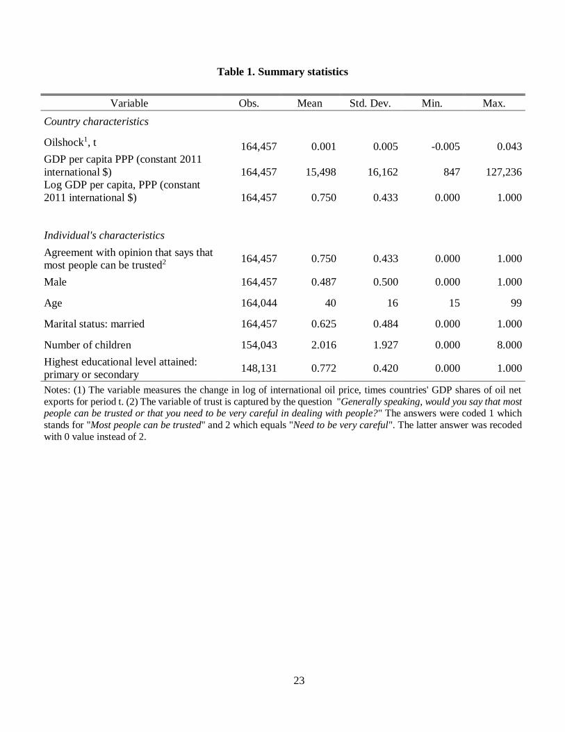
Table 1. Summary statistics
Variable Obs. Mean Std. Dev. Min. Max.
Country characteristics
Oilshock1, t 164,457 0.001 0.005 -0.005 0.043
GDP per capita PPP (constant 2011
international $)
164,457
15,498
16,162 847
127,236
Log GDP per capita, PPP (constant
2011 international $)
164,457 0.750 0.433 0.000 1.000
Individual's characteristics
Agreement with opinion that says that
most people can be trusted2 164,457 0.750 0.433 0.000 1.000
Male 164,457 0.487 0.500 0.000 1.000
Age 164,044 40 16 15 99
Marital status: married 164,457 0.625 0.484 0.000 1.000
Number of children 154,043 2.016 1.927 0.000 8.000
Highest educational level attained:
primary or secondary 148,131 0.772 0.420 0.000 1.000
Notes: (1) The variable measures the change in log of international oil price, times countries' GDP shares of oil net
exports for period t. (2) The variable of trust is captured by the question "Generally speaking, would you say that most people can be trusted or that you need to be very careful in dealing with people?" The answers were coded 1 which
stands for "Most people can be trusted" and 2 which equals "Need to be very careful". The latter answer was recoded
with 0 value instead of 2.

24
Table 2. Effects of country's per capita GDP on trust in people, probit results
Dependent variable Trust in people
(1) (2) (3)
Log GDP per capita, PPP (constant 2011 international $) 0.097* 0.099* 0.193***
(0.057) (0.057) (0.070)
Male -0.114 0.227***
(0.088) (0.010)
Age in years -0.000 -0.000
(0.000) (0.000)
Number of children -0.004*
(0.003)
Marital status
Married -0.0312*** -0.0291***
(0.008) (0.009)
Highest educational level attained
Primary or secondary complete/incomplete 0.227***
(0.009)
Fixed effects
Country Yes Yes Yes
Survey year Yes Yes Yes
Observations 164,457 164,044 138,037
LR chi2 13,531 13,543 12,573
Prob > chi2 0.000 0.000 0.000
Log likelihood -85,162 -84,935 -70,975 Notes: The method of estimation is maximum likelihood estimation. The observations are at the
individual-level unit. The dependent variable is measured with the question: "Generally speaking, would you say that most people can be trusted or that you need to be very careful in dealing with people?"
where the value 0 stands for "Need to be very careful" and 1 stands for "Most people can be trusted".
Coefficients that are significantly different from zero are denoted by the following system: * = 10%; ** = 5%; *** = 1%.

25
Table 3. Effects of country's per capita GDP on trust in people, IV results
(IV: Contemporaneous oil price shock, t)
Trust in people
(1) (2) (3)
Log GDP per capita, PPP (constant 2011 international $) 0.973*** 1.005*** 1.465*** (0.234) (0.234) (0.292)
Male -0.023*** -0.0177** (0.007) (0.00770) Age in years -0.000* -0.000319 (0.000) (0.000296) Marital status Married -0.0309*** -0.0284*** (0.008) (0.00895) Number of children -0.00493* (0.00267) Highest educational level attained Primary or secondary complete/incomplete 0.232*** (0.00914)
Fixed effects
Country Yes Yes Yes
Survey year Yes Yes Yes
Observations 164,457 164,044 138,037 Log pseudolikelihood 153,288 152,802 146,285
Wald chi-squared 13,617 13,635 12,697 Model Wald p-value 0.000 0.000 0.000 Wald chi-squared test of exogeneity 14.83 15.85 20.09 Wald test exogeneity p value 0.000 0.000 0.000
Notes: The method of estimation is maximum likelihood estimation. The observations are at the individual-
level unit. The dependent variable is measured with the question: "Generally speaking, would you say that most people can be trusted or that you need to be very careful in dealing with people?" where the value 0 stands for
"Need to be very careful" and 1 stands for "Most people can be trusted". Standard errors in parentheses.
Coefficients that are significantly different from zero are denoted by the following system: * = 10%; ** = 5%; *** = 1%.

26
Table 4. Effects of country's per capita GDP on trust in people, IV results
(IV: Lagged values of oil price shock t-1)
Trust in people
(1) (2) (3)
Log GDP per capita, PPP (constant 2011 international $) 1.239*** 1.325*** 1.846*** (0.421) (0.421) (0.445)
Male -0.0242*** -0.019**
(0.00704) (0.008)
Age in years -0.000441* -0.000
(0.000239) (0.000)
Marital status
Married -0.0311*** -0.029***
(0.00771) (0.009)
Number of children -0.005*
(0.003)
Highest educational level attained
Primary or secondary complete/incomplete 0.233***
(0.009) Fixed effects
Country Yes Yes Yes Survey year Yes Yes Yes Observations 162,459 162,046 136,047 Log pseudolikelihood 146,877 146,397 140,718 Wald chi-squared 13,657 13,689 12,752 Model Wald p-value 0.000 0.000 0.000
Wald chi-squared test of exogeneity 7.460 8.591 13.99 Wald test exogeneity p-value 0.006 0.003 0.000 Notes: The method of estimation is maximum likelihood estimation. The observations are at the individual-level
unit. The dependent variable is measured with the question: "Generally speaking, would you say that most people
can be trusted or that you need to be very careful in dealing with people?" where the value 0 stands for "Need to be very careful" and 1 stands for "Most people can be trusted". Standard errors in parentheses. Coefficients that
are significantly different from zero are denoted by the following system: * = 10%; ** = 5%; *** = 1%.
27
Table 5. Effects of country's per capita GDP on trust in people, IV results
(IV: Lagged values of oil price shock t-2)
Trust in people
(1) (2) (3)
Log GDP per capita, PPP (constant 2011 international $) 1.382*** 1.420*** 2.310*** (0.501) (0.502) (0.763)
Male -0.026*** -0.022***
(0.007) (0.008)
Age in years -0.000 -7.94e-05
(0.000) (0.000)
Marital status
Married -0.035*** -0.033***
(0.008) (0.009)
Number of children -0.005**
(0.003)
Highest educational level attained
Primary or secondary complete/incomplete 0.236***
(0.009) Fixed effects
Country Yes Yes Yes Survey year Yes Yes Yes Observations 156,790 156,377 130,406 Wald chi-squared 13,578 13,599 12,683 Model Wald p-value 0.000 0.000 0.000 Wald chi-squared test of exogeneity 7.456 7.802 8.612 Wald test exogeneity p-value 0.006 0.005 0.003
Notes: The method of estimation is maximum likelihood estimation. The observations are at the individual-level
unit. The dependent variable is measured with the question: "Generally speaking, would you say that most people can be trusted or that you need to be very careful in dealing with people?" where the value 0 stands for "Need to
be very careful" and 1 stands for "Most people can be trusted". Standard errors in parentheses. Coefficients that
are significantly different from zero are denoted by the following system: * = 10%; ** = 5%; *** = 1%.

28
Table 6. Effects of country's per capita GDP on trust in people, IV results
(IV: Contemporaneous values and lagged values of oil price shock; t and t-1)
Trust in people
(1) (2) (3)
Log GDP per capita, PPP (constant 2011 international $) 0.875*** 0.891*** 1.360*** (0.217) (0.217) (0.282)
Male -0.024*** -0.0189** (0.007) (0.008) Age in years -0.000* -0.000 (0.000) (0.000) Marital status Married -0.031*** -0.0294*** (0.008) (0.009) Number of children -0.005* (0.003) Highest educational level attained Primary or secondary complete/incomplete 0.232*** (0.009) Fixed effects Country FE Yes Yes Yes Survey year FE Yes Yes Yes Observations 162,459 162,046 136,047 Log pseudolikelihood 151,166 150,689 143,476 Wald chi-squared 13597 13,612 12,666 Model Wald p-value 0.000 0.000 0.000
Wald chi-squared test of exogeneity 13.77 14.29 18.21 Wald test exogeneity p-value 0.000 0.000 0.000
Notes: The method of estimation is maximum likelihood estimation. The observations are at the individual-
level unit. The dependent variable is measured with the question: "Generally speaking, would you say that
most people can be trusted or that you need to be very careful in dealing with people?" where the value 0 stands for "Need to be very careful" and 1 stands for "Most people can be trusted". Standard errors in
parentheses. Coefficients that are significantly different from zero are denoted by the following system: * =
10%; ** = 5%; *** = 1%.
29
Table 7. Effects of country's per capita GDP on trust in people, IV results
(IV: Contemporaneous values and lagged values of oil price shock; t, t-1 and t-2)
Trust in people (1) (2) (3)
Log GDP per capita, PPP (constant 2011 international $) 0.730*** 0.740*** 1.384*** (0.197) (0.197) (0.292)
Male -0.023*** -0.021*** (0.007) (0.008) Age in years -0.000 -0.000 (0.000) (0.000) Marital status Married -0.035*** -0.034*** (0.008) (0.0095) Number of children -0.005* (0.003) Highest educational level attained Primary or secondary complete/incomplete 0.235*** (0.009) Fixed effects Country FE Yes Yes Yes Survey year FE Yes Yes Yes Observations 156,790 156,377 130,406 Log pseudolikelihood 160,624 160,118 160,360 Wald chi-squared 13,496 13,511 12,559 Model Wald p-value 0.000 0.000 0.000 Wald chi-squared test of exogeneity 14.32 14.58 21.86 Wald test exogeneity p-value 0.000 0.000 0.000 Notes: The method of estimation is maximum likelihood estimation. The observations are at the individual-level unit. The dependent variable is measured with the question: "Generally speaking, would you say that most people can be trusted or that you need to be very careful in dealing with people?" where the value 0 stands for "Need to be very careful" and 1 stands for "Most people can be trusted". Standard errors in parentheses. Coefficients that are significantly different from zero are denoted by the following system: * = 10%; ** = 5%; *** = 1%.
30
Appendix A. List of countries included in baseline sample
1 ALB Albania 41 NGA Nigeria 2 DZA Algeria 42 NOR Norway 3 ARM Armenia 43 PAK Pakistan 4 AUS Australia 44 PER Peru 5 AZE Azerbaijan 45 PHL Philippines 6 BGD Bangladesh 46 POL Poland 7 BLR Belarus 47 QAT Qatar 8 BRA Brazil 48 ROU Romania 9 BGR Bulgaria 49 RWA Rwanda
10 BFA Burkina Faso 50 SGP Singapore 11 CAN Canada 51 SVN Slovenia 12 CHL Chile 52 ZAF South Africa 13 COL Colombia 53 ESP Spain 14 HRV Croatia 54 TZA Tanzania 15 CYP Cyprus 55 THA Thailand 16 SLV El Salvador 56 TUR Turkey 17 EST Estonia 57 UGA Uganda 18 ETH Ethiopia 58 UKR Ukraine 19 FIN Finland 59 USA United States 20 FRA France 60 URY Uruguay 21 GEO Georgia 61 ZMB Zambia 22 DEU Germany 62 ZWE Zimbabwe 23 GHA Ghana 24 GTM Guatemala 25 HUN Hungary 26 IND India 27 IDN Indonesia 28 IRQ Iraq 29 ISR Israel 30 ITA Italy 31 JPN Japan 32 JOR Jordan 33 LVA Latvia 34 LTU Lithuania 35 MYS Malaysia 36 MLI Mali 37 MEX Mexico 38 MAR Morocco 39 NLD Netherlands 40 NZL New Zealand
Source: World Value Survey (WVS), longitudinal dataset, 1981-2014.

31
Appendix B. Description of variables
Variable name Description
Dependent variable
Log GDP per capita, PPP
(constant 2011
international $)
Annual real per capita GDP measured in constant
international dollars from 2011. Current dollars
were converted using purchasing power parity
(PPP) rates based on the 2011 International
Comparison Round (ICP). Then, the log values
were taken.
Variable of interest
Agreement with opinion
that says that most people
can be trusted
The information is taken by the question:
"Generally speaking, would you say that most
people can be trusted or that you need to be very
careful in dealing with people?" The original
answers were coded 1 which stands for "Most
people can be trusted" and 2 which equals "Need to
be very careful". These values were recoded into a
dichotomous variable that takes the value of 1 and
0, respectively.
Instrument
Oilshock, t
Natural logarithm of the simple average of oil prices
from the Dubai, Brent and Texas report
(UNCTAD), multiplied by the share of net oil
exports in GDP.
Control variables
Male Dichotomous variable; has the value of 1 to indicate
“Men” and 0 otherwise.
Age Continuous variable that reports individual ages in
years.
Marital status: married Dichotomous variable; has a value of 1 to indicate
“Married” and 0 otherwise.
Number of children Continuous variable.
Highest educational level
attained
Dichotomous variable; has the value of 1 to indicate
“Primary or Secondary complete/incomplete” and 0
otherwise.
Survey year
Year in which the individual reported. Transformed
into dichotomous variable to indicate each year
value and control for fixed effects.
Country of residence
Country in which the individual lives when he or
she answered the WVS. Transformed into
dichotomous variable to indicate each country
control for fixed effects.
32
Appendix C. Trust and GDP: Interaction terms with OECD country members
Trust in people
(1) (2) (3)
OECD country member (=1) 0.873 0.954 -1.784
(0.715) (0.716) (1.114)
Log GDP per capita, PPP (constant
2011 international $)
0.106* 0.109* 0.215***
(0.0575) (0.0575) (0.0722)
OECD country member (=1)*Log
GDP per capita
-0.130* -0.138** 0.117
(0.0666) (0.0666) (0.100)
Constant -0.326 -0.296 -1.416**
(0.496) (0.496) (0.632)
Fixed effects
Country Yes Yes Yes
Survey year Yes Yes Yes
Observations 164,457 164,044 138,037
LR chi2 12579 12579 12579
Prob > chi2 0.000 0.000 0.000
Log likelihood -70974 -70974 -70974
Note: The method of estimation is probit. The observations are at an individual-level unit.
Standard errors in parentheses. Covariates follow the same specification as in previous tables. In column (1) there are no additional control variables. In column (2) control
variables are: male, age in years and marital status. Column (3) has the same covariates
as column (2) and adds the number of children and the highest educational level attained. Coefficients that are significantly different from zero are denoted by the following
system: * = 10%; ** = 5%; *** = 1%.

33
Appendix D. Weak instrument robust tests and confidence sets for IV probit
Test Panel A. Instrumental variable Oilshock, t
(1) (2) (3)
AR 17.28*** 18.41*** 25.54***
[ .512, 1.430] [ .551, 1.463] [ .904, 2.033]
Wald 17.25*** 18.38*** 25.48***
[ .515, 1.434] [ .547, 1.467] [ .898, 2.038]
Panel B. Instrumental variable Oilshock, t-1
(1) (2) (3)
AR 8.57*** 9.79*** 17.16***
[ .418, 2.066] [ .504, 2.154] [ .983, 2.722]
Wald 8.55*** 9.77*** 17.09***
[ .410, 2.075] [ .496, 2.162] [ .974, 2.73]
Panel C. Instrumental variable Oilshock, t-2
(1) (2) (3)
AR 7.47*** 7.85*** 8.97***
[ .401, 2.372] [ .437, 2.412] [ .814, 3.830]
Wald 7.45*** 7.83*** 8.92***
[ .391, 2.382] [ .426, 2.422] [ .798, 3.845]
Panel D. Instrumental variable Oilshock, t and t-1
(1) (2) (3)
CLR 16.19*** 16.80*** 23.47***
[ .453, 1.298] [ .469, 1.314] [ .816, 1.908]
K 16.19*** 16.80*** 23.47***
[ .453, 1.298] [ .469, 1.314] [ .816, 1.908]
AR 17.41*** 18.48*** 25.72***
[ .401, 1.320] [ .452, 1.331] [ .838, 1.886]
Wald 16.17*** 16.78*** 23.42***
[ .449, 1.302] [ .465, 1.3182] [ .811, 1.914]
Panel E. Instrumental variable Oilshock, t, t-1 and t-2
(1) (2) (3)
CLR 13.59*** 13.96*** 22.37***
[ .345, 1.114] [ .355, 1.124] [ .817, 1.955]
K 13.58*** 13.95*** 22.36***
[ .345, 1.114] [ .355, 1.124] [ .817, 1.955]
AR 16.89*** 17.89*** 25.05***
[ .3140, 1.145] [ .355, 1.124] [ .724, 2.048]

34
Wald 13.57*** 13.94*** 22.32***
[ .3415, 1.118] [ .351, 1.128] [ .811, 1.961]
Notes: Tests are computed within a non-linear two-step estimation framework allowing for
an endogenous repressor. Statistics confidence level follows the system: 10% = *; 5%=**;
1%=***. Confidence sets are presented in brackets. These are computed with confidence
levels of 95%, for 100 points across a range with the method of minimum distance (MD).
Homoscedastic standard errors are assumed for computation.

35
Recommended