East Tennessee State UniversityDigital Commons @ East
Tennessee State University
Electronic Theses and Dissertations Student Works
8-2012
As the Crow Flies: An Underrepresentation ofFood Deserts in the Rural Appalachian MountainsKasie RichardsEast Tennessee State University
Follow this and additional works at: https://dc.etsu.edu/etd
Part of the Policy Design, Analysis, and Evaluation Commons
This Dissertation - Open Access is brought to you for free and open access by the Student Works at Digital Commons @ East Tennessee StateUniversity. It has been accepted for inclusion in Electronic Theses and Dissertations by an authorized administrator of Digital Commons @ EastTennessee State University. For more information, please contact [email protected].
Recommended CitationRichards, Kasie, "As the Crow Flies: An Underrepresentation of Food Deserts in the Rural Appalachian Mountains" (2012). ElectronicTheses and Dissertations. Paper 1453. https://dc.etsu.edu/etd/1453
As the Crow Flies: An Underrepresentation of Food Deserts in the Rural Appalachian Mountains
____________________
A dissertation presented to
the faculty of the College of Public Health East Tennessee State University
In partial fulfillment of the requirements for the degree
Doctor of Public Health with a concentration in
Community and Behavioral Health
____________________
by Kasie Richards August 2012
____________________
Dr. Deborah Slawson, Chair Dr. Arsham Alamian
Dr. Ke Chen
Keywords: Appalachian, “food desert”, “food access”, “food availability”, GIS
2
ABSTRACT
As the Crow Flies: An Underrepresentation of Food Deserts in the Rural Appalachian Mountains
by
Kasie Richards
Diet and dietary related health outcomes such as obesity and diabetes are major public health
concerns. While personal choice and dietary behaviors are major influences on how an
individual eats, the environment influences these choices and behaviors. The nutrition
environment is one key influence and its relationship with food choice, behaviors, and
socioeconomic influences is complex. Within the structure of the nutrition environment, food
access and socioeconomic status compound influencing nutrition behavior and food choice.
Food deserts are defined as geographic region of low access to healthy affordable food in low
income areas. The USDA developed a system for the analysis of food deserts in the United
States. However, the methods the USDA uses do not acknowledge potential geographical
barriers present in rural mountainous regions including Appalachia. The purpose of this research
is to determine whether the USDA methodology underrepresents food deserts in Appalachia and
to develop a modified analysis model for the region.
The region was analyzed at the census tract level using methods based on USDA guidelines for
low income, rurality, and grocery store identification, then applied in Geographic Information
Systems (GIS) to roadway data. Network analysis of drive time from grocery stores to 20
minutes away was performed. Low income, rural census tracts with 33% of their area outside of
3
the 20-minute drive time zone were identified as food deserts. Counties containing tracts were
then compared to USDA designated counties, using the dependent variables of obesity and
diabetes diagnosis rates and controlled for by county level rurality and economic distress.
Of the counties designated as rural, 63 contained food deserts by the modified methods and the
USDA model identified 20, there was an overlap in identification of 12 counties. There was no
significant difference for 2 methods in health outcomes for the counties.
In conclusion, the modified methods do identify a larger food desert region. It is crucial to
understand the geographic barriers to regions when addressing nutrition environment concerns.
The underrepresentation of food desert areas can leave populations and communities
underserved and without much needed resources to improve their access to healthy and
affordable foods.

4
DEDICATION
To Cory: for his logic and levity.

5
ACKNOWLEDGEMENTS
Thank you to: Dr. Deborah Slawson my mentor for patience, support, confidence, and
guidance; to my dissertation committee (Dr. Chen and Dr. Alamian) and my academic
committee (Dr. Pack and Dr. Bounds) for knowledge, support, and fortitude; Dr. Chris Gregg for
mentorship; to the ETSU College of Public Health and my friends and family.
6
CONTENTS
Page
ABSTRACT .................................................................................................................................... 2
DEDICATION ................................................................................................................................ 4
ACKNOWLEDGEMENTS ............................................................................................................ 5
LIST OF TABLES ........................................................................................................................ 10
LIST OF FIGURES ...................................................................................................................... 11
LIST OF ABBREVIATIONS ....................................................................................................... 12
Chapter
1. INTRODUCTION ............................................................................................................ 13
Food Deserts ......................................................................................................... 13
USDA Food Desert Locator...................................................................... 13
Geographic Information Systems (GIS) ................................................... 14
Food Access .......................................................................................................... 14
The Appalachian Region ....................................................................................... 16
Significance........................................................................................................... 16
Research Purpose .................................................................................................. 17
Specific Aims ........................................................................................................ 17
Specific Aim 1 .......................................................................................... 17
Specific Aim 2 .......................................................................................... 17
7
Specific Aim 3 .......................................................................................... 18
Research Hypotheses ............................................................................................ 18
Hypothesis 1.............................................................................................. 18
Hypothesis 2.............................................................................................. 18
2. 2.LITERATURE REVIEW .............................................................................................. 19
Theoretical Framework ......................................................................................... 19
Neighborhood Deprivation and Food Environment ............................................. 23
Health Outcomes and Food Environment ............................................................. 25
Rural Food Environment ...................................................................................... 28
Fruit and Vegetable Availability and Intake ......................................................... 31
Spatial Analysis .................................................................................................... 34
Conclusion ............................................................................................................ 37
3. METHODS ....................................................................................................................... 39
Data Used .............................................................................................................. 39
Sample Selection ................................................................................................... 40
Why Appalachia? ...................................................................................... 40
Regional Economics ................................................................................. 41
Economic Distress .................................................................................... 42
Rural Urban Commuting Area Codes ....................................................... 44
8
Analysis................................................................................................................. 49
Data and Mapping Methodology .............................................................. 49
Statistical Analysis .................................................................................... 52
Dependent Variables ................................................................................. 52
Independent Variables .............................................................................. 54
4. RESULTS ......................................................................................................................... 56
Descriptive Data.................................................................................................... 56
Rural Designation ................................................................................................. 62
Economic Distress ................................................................................................ 63
Food Access .......................................................................................................... 64
Comprehensive Models ........................................................................................ 68
Health Outcomes ................................................................................................... 71
Obesity ...................................................................................................... 71
Diabetes..................................................................................................... 74
5. DISCUSSION ................................................................................................................... 77
Summary ............................................................................................................... 77
Reproducibility ..................................................................................................... 78
Food Access .......................................................................................................... 78
Food Outlets .............................................................................................. 78
9
Drive Time ................................................................................................ 80
Defining Rural ...................................................................................................... 82
Income Status ........................................................................................................ 83
Study Limitations .................................................................................................. 83
Future Studies ....................................................................................................... 85
Contribution to Public Health ............................................................................... 86
REFERENCES ............................................................................................................................. 87
APPENDIX: IRB Exemption ....................................................................................................... 97
VITA ............................................................................................................................................. 98
10
LIST OF TABLES
Table Page
1: Rural Urban Continuum Codes (USDA, 2004) ................................................................... 46
2: Descriptive Data on Food Desert Designations ................................................................... 58
3: Distribution of Counties for Food Desert Methods .............................................................. 59
4: Comparative County Level Obesity Diagnosis Estimates for Food Desert Methods .......... 73
5: Regression Analysis for Obesity Estimates ......................................................................... 73
6: Comparative County Level Diabetes Diagnosis Estimates for Food Desert Methods ........ 75
7: Regression Analysis for Diabetes Estimates ........................................................................ 76
11
LIST OF FIGURES
Figure Page
1: Socioecologial Framework ................................................................................................. 22
2: Metropolitan and Micropolitan Statistical Areas ................................................................ 47
3: USDA Rural Designation: < 2,500 Census Tract Residents ............................................... 48
4: USDA Identified Food Desert Census Tracts ..................................................................... 60
5: Drive Time Modified Food Desert Census Tracts .............................................................. 61
6: Low Income Designated Census Tracts .............................................................................. 65
7: USDA Methodology - 10 Mile Buffer Analysis ................................................................. 66
8: Modified Methodology - 20 Minute Drive Time Analysis ................................................. 67
9: USDA Methodology Model................................................................................................ 69
10: Modified Methodology Model.......................................................................................... 70

12
LIST OF ABBREVIATIONS
United States Department of Agriculture (USDA)
Environmental Systems Research Institute, Inc. (Esri)
North American Industry Classification System (NAICS)
U.S. Economic Classification Policy Committee (ECPC)
Retail Food Environment Index (RFEI)
Body Mass Index (BMI)
Healthy Eating Indicator Shopping Basket (HEISB)
United Kingdom’s (UK)
American Community Survey (ACS)
Topographically Integrated Geographic Encoding and Referencing system (TIGER)
North Carolina Department of Transportation (NCDOT)
Women, Infant Child (WIC)
Center for Disease Control and Prevention’s (CDC’s)
National Diabetes Surveillance System (NDSS)
National Index Value (NIV)
Rural urban commuting area (RUCA)
White House’s Office of Management and Budget (OMB)
Core Based Statistical Areas (CBSA’s)
Universal Transverse Mercator (UTM)
Behavioral Risk Factor Surveillance Survey (BRFSS)
13
CHAPTER 1
INTRODUCTION
Food Deserts
“Food deserts” are characterized by poor access to healthy and affordable food (Beaulac,
Kristjansson, & Cummins, 2009; USDA: Economic Research Services, 2011). While the
defining factor of a food desert is often considered the literal absence of retail food within an
area, it is predominately studied under the context of regional socioeconomic status as well
(Beaulac et al., 2009). Food deserts can be used to assess food access and affordability as it
relates to both socioeconomically advantaged and disadvantaged populations (Beaulac et al.,
2009; Story, Kaphingst, Robinson-O'Brien, & Glanz, 2008). Thus, it is commonly considered
that social disparities that exist in diet and diet related health outcomes could be related to the
occurrence of food deserts (Cummins & Macintyre, 2006; Powell & Bao, 2009; Wrigley, Warm,
& Margetts, 2003; Zenk et al., 2005).
USDA Food Desert Locator
The United States Department of Agriculture (USDA) defines a food desert as a low
income census tract where a substantial portion of the residents have low access to a supermarket
or large grocery store (USDA: Economic Research Services, 2011). As part of First Lady
Michelle Obama’s “Lets’ Move” initiative, the Healthy Food Financing Initiative set the goal to
expand the availability of nutritious food to food desert regions (USDA: Economic Research
Services, 2011). As part of this goal, the Food Desert Locator and its prescribed methodology
for food desert identification was developed based upon findings from a 2009 report to Congress
on food deserts (USDA: Economic Research Services, 2011). The Food Desert Locator was
14
introduced by Agriculture Secretary Tom Vilsack on May 2, 2011, as a tool to aid community
planners, policy makers, researchers, and others identify communities in need of interventions to
improve access to healthy affordable foods (USDA, 2011).
Geographic Information Systems (GIS)
Geographic Information System (GIS) is an integrative system of hardware, data, and
software that is used to capture, manage, analyze, and display any form of geographically
referenced information (Environmental Systems Research Institute, Inc. (Esri), 2012).
Geographically referenced data can include many different forms including point location data,
boundary lines, image files, and data associated with a location. This associated or referenced
data can include census data and statistics that have corresponding codes for country, state,
county, census tract, or address. This leads GIS to be a useful tool for many research
environments including public health. GIS have become more popular with regards to assessing
built environment, including food environments (Glanz, Sallis, Saelens, & Frank, 2005;
McKinnon, Reedy, Handy, & Rodgers, 2009; Wendel-Vos, Droomers, Kremers, Brug, & van
Lenthe, 2007). It is a frequently used tool in the measure and assessment of disparities related to
health access (McLafferty, 2003) and its use in the development of standards for identifying food
desert regions has become common practice (Forsyth, Lytle, & Van Riper, 2010; Sharkey, Horel,
& Dean, 2010; USDA: Economic Research Services, 2011).
Food Access
The consumer nutrition environment reflects the availability and access of healthy foods.
The consumer nutrition environment is defined as the environment in and around where food is
purchased and can include options, price, promotion, placement, and even nutritional
15
information that can also influence food choice (Glanz et al., 2005). The environment that the
consumer is exposed to influences choice. Environmental factors influencing food choice and
nutrition behaviors may put populations at a greater risk for chronic disease.
Spatial access to healthy foods is considered an influence on food choice and thus
impacts one’s risk of chronic disease (Glanz et al., 2005; Hill & Peters, 1998; Larson, Story, &
Nelson, 2009; White, 2007; Papas et al., 2007). Spatial access is a subset of the consumer
nutrition environment referred to as the community food environment. This community food
environment can be described as spatial access to food that includes the number, location, type,
and accessibility of food outlets to a community or neighborhood (Glanz et al., 2005). Food
outlets can include a variety of stores, not only supermarkets and grocery stores, but restaurants
and convenience stores as well (Glanz et al., 2005). Food outlet type is based on North
American Industry Classification System (NAICS) coding for retail markets that separates large
supermarkets and chain grocery stores from convenience stores and smaller markets (Blanchard
& Lyson, 2002; McEntee & Agyeman, 2009).
In more rural communities there are fewer large supermarket options and food access is
comprised primarily of independent grocery and convenience stores (Black & Macinko, 2008;
Smith et al., 2010). This trend towards independent grocery and convenience stores has also
been found to be true in neighborhoods with lower socioeconomic status (Beaulac et al., 2009;
Black & Macinko, 2008; Cummins & Macintyre, 2006; Smith et al., 2010; USDA: Economic
Research Services, 2012; White, 2007). Numerous reports have indicated that Americans living
in low income areas tend to have poorer access to healthy food (Beaulac et al., 2009; Black &
Macinko, 2008; Cummins & Macintyre, 2006; Smith et al., 2010; USDA: Economic Research
Services, 2012; White, 2007). It has been shown that as regions decrease in population density
16
and average income, the fewer large grocery markets, thus physically limiting food choice
(Beaulac et al., 2009; Hosler, 2009).This limited access to large supermarket access creates a
barrier because these smaller consumer markets tend to charge higher prices (Bitler & Haider,
2011; Black & Macinko, 2008; Story et al., 2008).
Higher prices in turn influence food choice. Energy dense nutritionally lacking foods
cost less than healthier options (Beaulac et al., 2009). This economic reality drives food choice
away from healthier options. For those individuals who are low income, the high expense of
healthy foods is a barrier to healthy food choices (Hamelin & Beaudry, 2002; Story et al., 2008;
Yousefian, Leighton, Fox, & Hartley, 2011).
The Appalachian Region
The Appalachian region reflects a population that is more rural than the US as a whole
with 42% of its residents living in rural areas (Appalachian Regional Commission, 2012). This
is more than double the current US rate of rural residents (Appalachian Regional Commission,
2012). Also, the Appalachian region continues to be an area of strong economic disadvantage
and contains more high poverty counties than the current US average (Appalachian Regional
Commission, 2012). With healthy food access concerns being linked to economic deprivation
and rural environments, the study of food deserts within the Appalachian region provides an
opportunity for strong representative analysis.
Significance
The development of spatial analysis measures that will better identify underrepresented at
risk populations with regard to food deserts and their related implications is a step towards the
necessary sustained public health effort needed to make healthy food accessible and affordable
17
for everyone (Story et al., 2008). It has become evident that to improve dietary behavior and
decrease obesity and dietary related diseases, efforts must be made to address the environmental
influences (Story et al., 2008). This research contributes to the field of public health by
investigating the growing concerns over food deserts considering their evident influence on
eating behaviors and food choices. This was accomplished by developing a methodology for
better representing rural mountainous populations in regard to their access to and the availability
of healthy foods.
Research Purpose
The purpose of this research is to determine if the current USDA standard for identifying
food desert regions underrepresents the access and availability of healthy and affordable foods in
rural Appalachian Mountains.
Specific Aims
Specific Aim 1
Develop a methodology for weighting or adjusting USDA Food Desert Designations
based on drive times.
Specific Aim 2
Determine if the addition of drive time to rural food desert designations increases the
overall area and number of food desert regions identified when compared to USDA Food Desert
Designations.
18
Specific Aim 3
Compare county health indicators and outcomes from counties identified containing one
or more food desert regions using the USDA designations with those counties identified using
travel time modified results.
Research Hypotheses
Hypothesis 1
It is hypothesized that there will be an increase in the overall area and number of food
desert regions identified when the standard 10 mile radius buffer used by USDA Food Desert
Mapping is replaced with a network analysis of driving time.
Hypothesis 2
It is hypothesized that the county health indicator and outcome status of the newly
identified food desert regions will reflect similar health indicators and outcomes as those already
identified as food desert regions by the USDA Food Desert Mapping.
19
CHAPTER 2
LITERATURE REVIEW
Theoretical Framework
The relationship among nutrition environments, socioeconomic influences, and individual
food choices and dietary behaviors is complex. The overarching theory that guides this work is
the socioecological model that addresses influences and relationships at the individual, family,
community, and governmental levels. A socioecological approach to food environment is useful
in describing the many spheres of influence that exist within its constructs (Hallett &
McDermott, 2010; Powell, Han, & Chaloupka, 2010; Story et al., 2008; White, 2007). It can
allow for the integrating of food intake influences into a comprehensive framework (Sallis et al.,
2009; Story et al., 2008). During the course of this research, we considered how food deserts
may affect home, community, and commercial aspects as well as its influence over individual
variables. Also, we will discuss how government and industry policies may help to alleviate the
impact of food deserts.
There are individual factors that influence healthy dietary behaviors; food choice is a
primary factor (Figure 1) (Glanz et al., 2005). Food choice is the single most influential factor
on healthy dietary behaviors (Glanz et al., 2005). At the individual level food choice can be
affected by behavioral and personal determinants including perceptions, knowledge, and beliefs
(Figure 1) (Story et al., 2008; Powell et al., 2010). In addition, food security, as well as social
demographics, plays a role in eating behavior and food choice (Figure 1) (Bitler & Haider, 2011;
Powell et al., 2010).
20
From the family or household level individual food choice is affected by what food is
provided in the household. Home food environment is a key contributor influencing individual
food environments (Figure 1) (Glanz et al., 2005). This reflects the foods that are provided for
access at home. The purchaser influences the diets of the entire household by providing their
individual choices to the family unit (Figure 1) (Glanz et al., 2005; Story et al., 2008; White,
2007). These purchaser choices are affected by the preferences of other members of the
household, tradition, and culture as well as knowledge and beliefs regarding healthy foods
(Figure 1) (Powell et al., 2010; Story et al., 2008).
The physical household environment can also play a role in food choice, including the
availability of proper food storage, preparation and cooking facilities, and equipment (Figure 1)
(Bitler & Haider, 2011; Story et al., 2008; White, 2007). Household income can also affect food
choice, if there are other financial priorities, or overall financial insecurity within the household,
the potential for a nutritious diet suffers (Bitler & Haider, 2011; White, 2007). At the
community level there are many environmental influences affecting food choice and thus diet
(Figure 1).
One of the primary sources of influence results from the physical environment of the
community (Figure 1). Where food is acquired and eaten can be influenced by aspects of the
physical environment including neighborhood geographic location and accessibility as well as by
neighborhood deprivation levels (Figure 1) (Glanz et al., 2005; Story et al., 2008). It has been
found that neighborhoods with increasing deprivation due to socioeconomic status (low income
and high rates of poverty) are often more susceptible to poor access and availability of healthy
foods (Bitler & Haider, 2011; Furey, Farley, & Strugnell, 2002; Powell et al., 2010). Thus,
21
living in these communities can physically affect an individual’s food choice and eating
behaviors (Glanz et al., 2005; Story et al., 2008; White, 2007).
At the overarching macro governmental and policy level there are powerful influences
that operate (Figure 1). These include the influence of food marketing and media as well as
social norms (Powell et al., 2010; Story et al., 2008). Other influences include food production
and distribution systems (Figure 1) (Bitler & Haider, 2011; Powell et al., 2010; Story et al.,
2008). Larger corporations that have the ability to purchase and ship food at lower costs and
thus provide lower cost food options are less likely to choose to put stores within geographically
remote and socioeconomically deprived neighborhoods, thus regionally and nationally creating
lower access and availability of healthy foods (Bitler & Haider, 2011; Furey et al., 2002; Powell
et al., 2010; Story et al., 2008). Current national and state agriculture policies can also affect the
access and availability of foods on a large scale (Figure 1).
Also at the macro level, food pricing structures have a significant impact on food choice
and eating behaviors. There is a need to understand the influence of economics on food deserts.
Economic theories suggest that the purchase of healthy foods increases as income level increases
(Bitler & Haider, 2011; Furey et al., 2002; White, 2007). With a lack of large supermarkets in
rural and deprived communities, smaller market options often fill the gaps (Cummins &
Macintyre, 2006; Day & Pearce, 2011). However, these smaller scale markets often find higher
overhead costs that in turn are passed on to the consumer, elevating the costs of food available to
those most vulnerable (Bitler & Haider, 2011; Powell et al., 2010; Yousefian et al., 2011).
Overall, a comprehensive system for identifying areas of limited food access and
availability within the Appalachian region is a critical element to addressing possible concerns of
nutrition adequacy in these areas. Regions of economic distress such as those found in
22
Appalachia are at an even greater risk for poor access and availability of healthy foods from a
socioeconomic and population density aspect. However, there are many areas that may fit the
profile of a food desert region within the Appalachian Mountains that are not represented under
the current geographic measurement system in that it does not reflect the topography and
population distributions of the region.
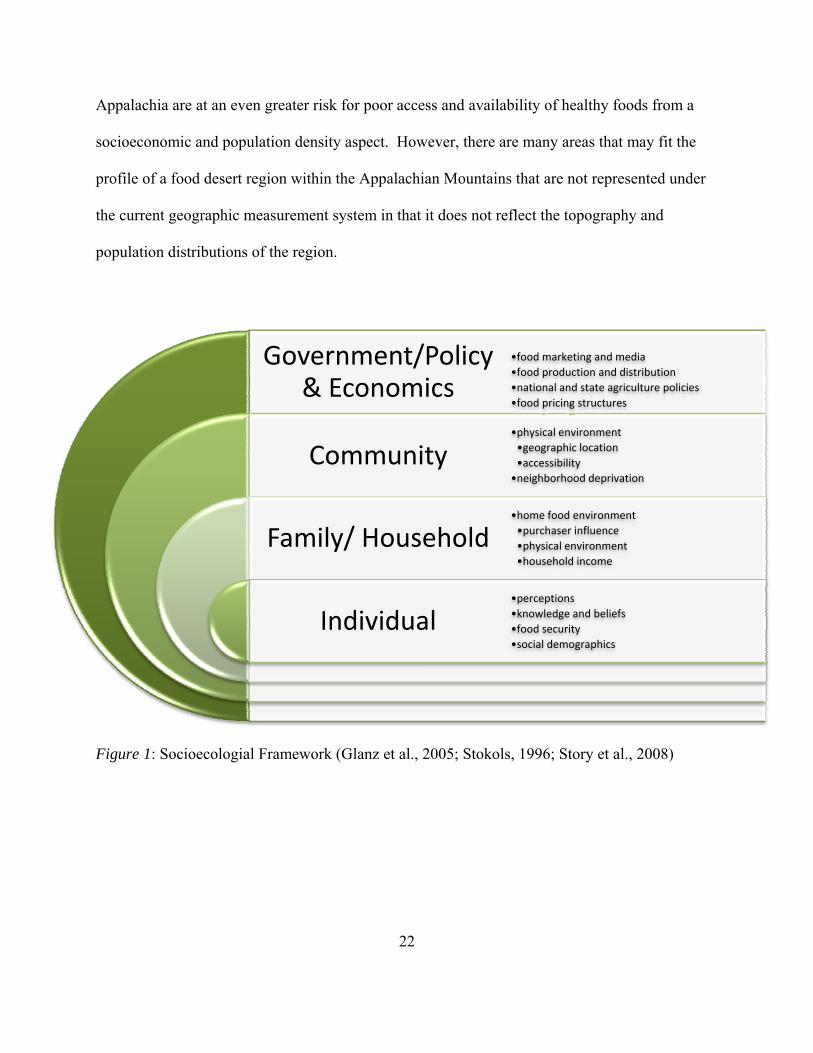
Figure 1: Socioecologial Framework (Glanz et al., 2005; Stokols, 1996; Story et al., 2008)
Government/Policy & Economics
Community
Family/ Household
Individual
•food marketing and media
•food production and distribution
•national and state agriculture policies
•food pricing structures
•physical environment
•geographic location
•accessibility
•neighborhood deprivation
•home food environment
•purchaser influence
•physical environment
•household income
•perceptions
•knowledge and beliefs
•food security
•social demographics
23
Neighborhood Deprivation and Food Environment
Many studies investigating food access and availability have found that socioeconomic
factors including low income and poverty are key factors in identifying low access and
availability to healthy foods (Ahern, Brown, & Dukas, 2011; Black & Macinko, 2008; Ford &
Dzewaltowski, 2011; Smith et al., 2010). Neighborhood deprivation has been significantly
associated with the presence of food deserts. Several reports have indicated that access to large
supermarkets is positively associated with socioeconomic level (Powell et al., 2010; Wang, Kim,
Gonzalez, MacLeod, & Winkleby, 2007). Thus, there are fewer large and chain supermarkets
and grocery stores in lower socioeconomic areas. There is also greater likelihood for low income
neighborhoods to have an increased number of small independent grocery stores, fast food
restaurants, and convenience stores (Bitler & Haider, 2011; Black & Macinko, 2008; Jilcott et
al., 2010; Story et al., 2008).
Sharkey, Horel, Han, and Huber, (2009) found that in high deprivation areas there are
fewer food stores and more convenience stores and fast food restaurants. By categorizing and
analyzing retail food sales locations and not only supermarkets and grocery stores, this study
contributes to a greater understanding of the multiple aspects of comprehensive food access
(Sharkey et al., 2009). Higher prices and more limited shopping options increase in prevalence
with an increased presence of smaller independently owned grocers and convenience stores
(Bitler & Haider, 2011; White, 2007). Overall these elevated prices and declining food outlet
options mean that communities with a lower the socioeconomic status are less likely to have
access to healthy and affordable food.
The variation in affordability and availability of healthy foods based on food outlet type
is one reason that North American Industry Classification System (NAICS) codes are used to aid
24
in delineating outlet type. This classification system is used by Federal agencies as the standard
in classifying business for use in research associated with the US business economy (US Census
Bureau, 2012). Developed jointly by U.S. Economic Classification Policy Committee (ECPC),
Statistics Canada, and Mexico's Instituto Nacional de Estadistica y Geografia, the NAICS was
adopted in 1997 in order to improve the ability to compare business statistics across all of North
America (US Census Bureau, 2012) .The NAICS codes allow for food outlet types to be
categorized in a way that excludes small independent grocery stores, convenience stores, and
restaurants from those classified as supermarkets and large chain grocery stores (Sharkey et al.,
2009; US Census Bureau, 2012). This may develop a better representation of a neighborhood’s
access to healthy and affordable food delineation. However, there is concern with these
consumer designations as multifunction stores become increasingly common.
A greater understanding of retail food sales is needed as the number of stores that would
otherwise be considered supermarkets and grocery stores expand their line services to prepared
food items (Sharkey, Johnson, Dean, & Horel, 2011). It is becoming more common to see fast
food entrees and sides served in nonfast food locations, including grocery and convenience stores
(Sharkey et al., 2011). While known that fast food restaurant density increases as neighborhood
deprivation increases, it has also come to light that there is an increased availability of fast food
style entrees and sides not associated with fast food restaurants available in or near
socioeconomically deprived neighborhoods (Sharkey et al., 2011). Away from home
consumption of fast food style products may contribute to the energy dense, low nutritional value
food choice in deprived neighborhoods (Sharkey et al., 2011).
Neighborhood deprivation has also been linked to BMI (Hosler, 2009; Jennings et al.,
2011; Powell et al., 2010). As neighborhood deprivation increases, so does the risk of
25
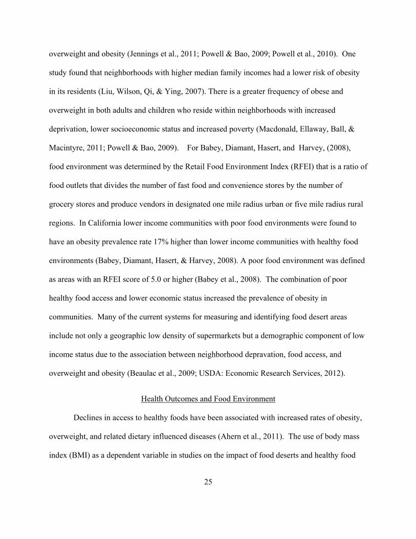
overweight and obesity (Jennings et al., 2011; Powell & Bao, 2009; Powell et al., 2010). One
study found that neighborhoods with higher median family incomes had a lower risk of obesity
in its residents (Liu, Wilson, Qi, & Ying, 2007). There is a greater frequency of obese and
overweight in both adults and children who reside within neighborhoods with increased
deprivation, lower socioeconomic status and increased poverty (Macdonald, Ellaway, Ball, &
Macintyre, 2011; Powell & Bao, 2009). For Babey, Diamant, Hasert, and Harvey, (2008),
food environment was determined by the Retail Food Environment Index (RFEI) that is a ratio of
food outlets that divides the number of fast food and convenience stores by the number of
grocery stores and produce vendors in designated one mile radius urban or five mile radius rural
regions. In California lower income communities with poor food environments were found to
have an obesity prevalence rate 17% higher than lower income communities with healthy food
environments (Babey, Diamant, Hasert, & Harvey, 2008). A poor food environment was defined
as areas with an RFEI score of 5.0 or higher (Babey et al., 2008). The combination of poor
healthy food access and lower economic status increased the prevalence of obesity in
communities. Many of the current systems for measuring and identifying food desert areas
include not only a geographic low density of supermarkets but a demographic component of low
income status due to the association between neighborhood depravation, food access, and
overweight and obesity (Beaulac et al., 2009; USDA: Economic Research Services, 2012).
Health Outcomes and Food Environment
Declines in access to healthy foods have been associated with increased rates of obesity,
overweight, and related dietary influenced diseases (Ahern et al., 2011). The use of body mass
index (BMI) as a dependent variable in studies on the impact of food deserts and healthy food
26
access and availability is common. It has been found that BMI is associated with many factors
related to unhealthy food environments (Ahern et al., 2011; Ford & Dzewaltowski, 2011;
Jennings et al., 2011; Powell & Bao, 2009; Powell et al., 2010; Schafft, Jensen, & Hinrichs,
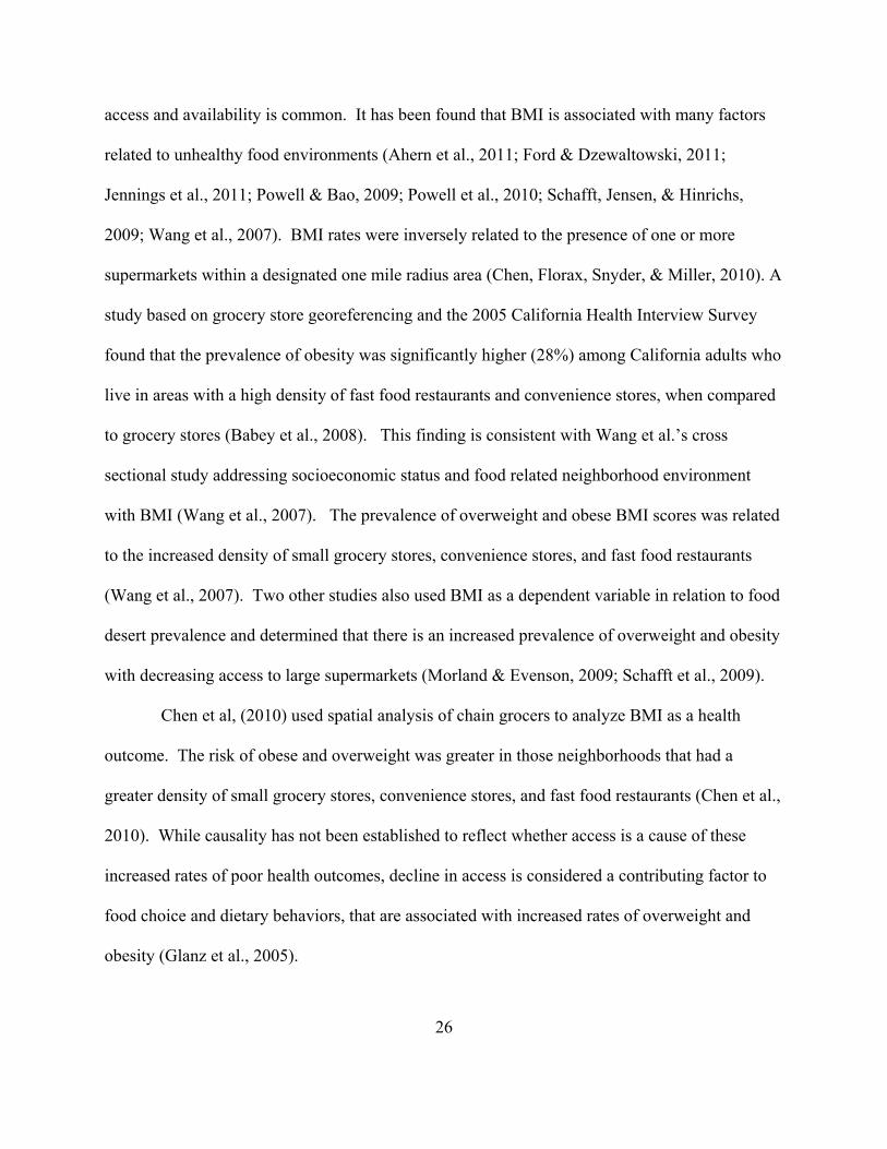
2009; Wang et al., 2007). BMI rates were inversely related to the presence of one or more
supermarkets within a designated one mile radius area (Chen, Florax, Snyder, & Miller, 2010). A
study based on grocery store georeferencing and the 2005 California Health Interview Survey
found that the prevalence of obesity was significantly higher (28%) among California adults who
live in areas with a high density of fast food restaurants and convenience stores, when compared
to grocery stores (Babey et al., 2008). This finding is consistent with Wang et al.’s cross
sectional study addressing socioeconomic status and food related neighborhood environment
with BMI (Wang et al., 2007). The prevalence of overweight and obese BMI scores was related
to the increased density of small grocery stores, convenience stores, and fast food restaurants
(Wang et al., 2007). Two other studies also used BMI as a dependent variable in relation to food
desert prevalence and determined that there is an increased prevalence of overweight and obesity
with decreasing access to large supermarkets (Morland & Evenson, 2009; Schafft et al., 2009).
Chen et al, (2010) used spatial analysis of chain grocers to analyze BMI as a health
outcome. The risk of obese and overweight was greater in those neighborhoods that had a
greater density of small grocery stores, convenience stores, and fast food restaurants (Chen et al.,
2010). While causality has not been established to reflect whether access is a cause of these
increased rates of poor health outcomes, decline in access is considered a contributing factor to
food choice and dietary behaviors, that are associated with increased rates of overweight and
obesity (Glanz et al., 2005).
27
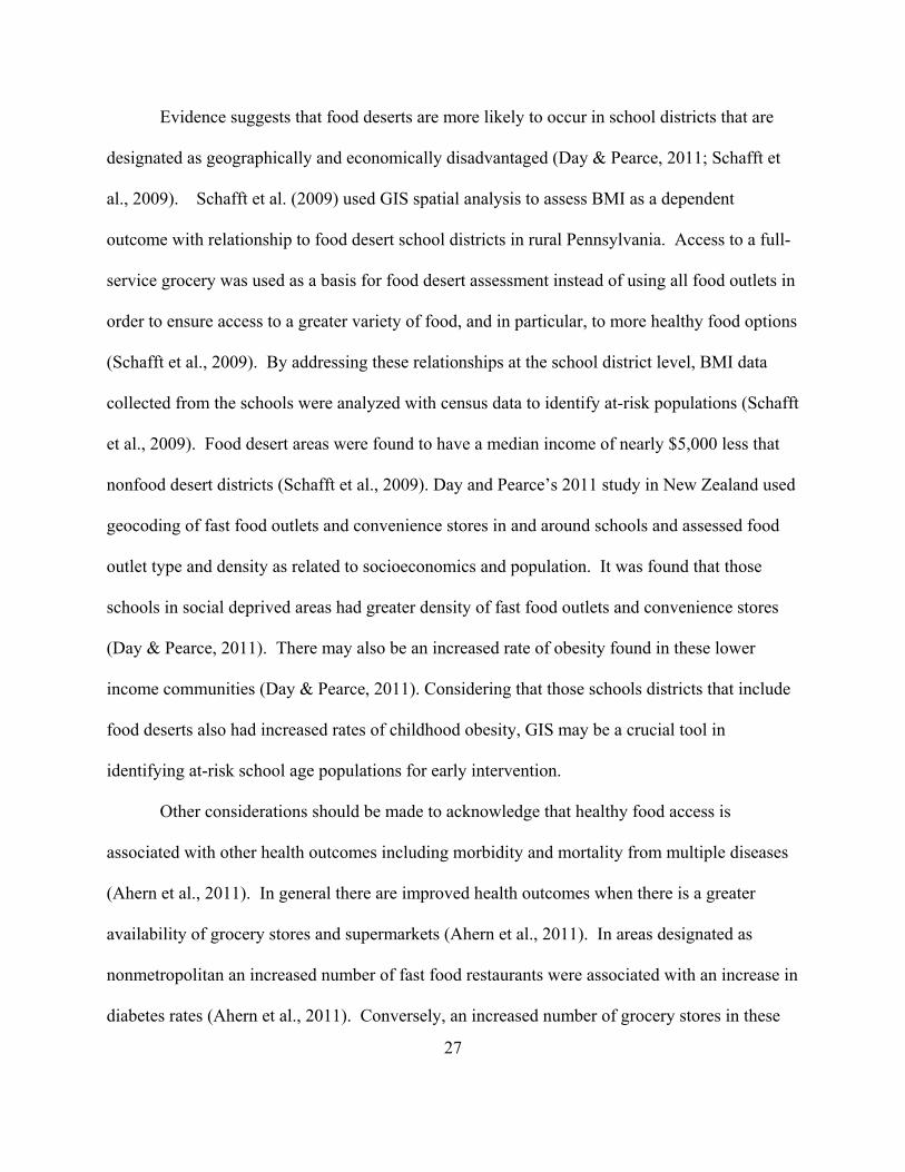
Evidence suggests that food deserts are more likely to occur in school districts that are
designated as geographically and economically disadvantaged (Day & Pearce, 2011; Schafft et
al., 2009). Schafft et al. (2009) used GIS spatial analysis to assess BMI as a dependent
outcome with relationship to food desert school districts in rural Pennsylvania. Access to a full-
service grocery was used as a basis for food desert assessment instead of using all food outlets in
order to ensure access to a greater variety of food, and in particular, to more healthy food options
(Schafft et al., 2009). By addressing these relationships at the school district level, BMI data
collected from the schools were analyzed with census data to identify at-risk populations (Schafft
et al., 2009). Food desert areas were found to have a median income of nearly $5,000 less that
nonfood desert districts (Schafft et al., 2009). Day and Pearce’s 2011 study in New Zealand used
geocoding of fast food outlets and convenience stores in and around schools and assessed food
outlet type and density as related to socioeconomics and population. It was found that those
schools in social deprived areas had greater density of fast food outlets and convenience stores
(Day & Pearce, 2011). There may also be an increased rate of obesity found in these lower
income communities (Day & Pearce, 2011). Considering that those schools districts that include
food deserts also had increased rates of childhood obesity, GIS may be a crucial tool in
identifying at-risk school age populations for early intervention.
Other considerations should be made to acknowledge that healthy food access is
associated with other health outcomes including morbidity and mortality from multiple diseases
(Ahern et al., 2011). In general there are improved health outcomes when there is a greater
availability of grocery stores and supermarkets (Ahern et al., 2011). In areas designated as
nonmetropolitan an increased number of fast food restaurants were associated with an increase in
diabetes rates (Ahern et al., 2011). Conversely, an increased number of grocery stores in these

28
same nonmetropolitan areas were linked with lower mortality and diabetes rates (Ahern et al.,
2011). Similar to Babey et al.’s 2008 finding on obesity prevalence, California adults with a
high density of fast food restaurants and convenience stores near their residences relative to
grocery stores had the highest prevalence of diabetes.
Thus, while determining whether the presence of food deserts is a causal factor for poor
health outcomes has not been addressed in the current literature; there is evidence to support
relationships between these factors. By identifying food deserts we can provide for more
community tailored intervention strategies and provide evidence based strategies for policy
change that may impact the growing epidemic of obesity in the United States.
Rural Food Environment
Rural neighborhoods are less likely to have access to large chain supermarkets and thus
rely on smaller independently owned grocers and convenience stores (Sharkey et al., 2010).
While causality has not been established, greater access to smaller grocers and convenience
stores is related to an increased prevalence of obesity in rural areas (Morland & Evenson, 2009).
Also, in lower population density areas, as distance to grocery stores increase, so does the risk of
overweight (Liu et al., 2007).
While the majority of food desert measures and research has targeted urban settings, rural
settings are gaining more attention. Rural food deserts create some unique concerns and barriers
to healthy food access. One crucial element is the amount of time it takes to drive to a large or
chain supermarket. Thomas found that 75% of households placed distance from home as the
most significant concern with grocery store access (Thomas, 2010).
29
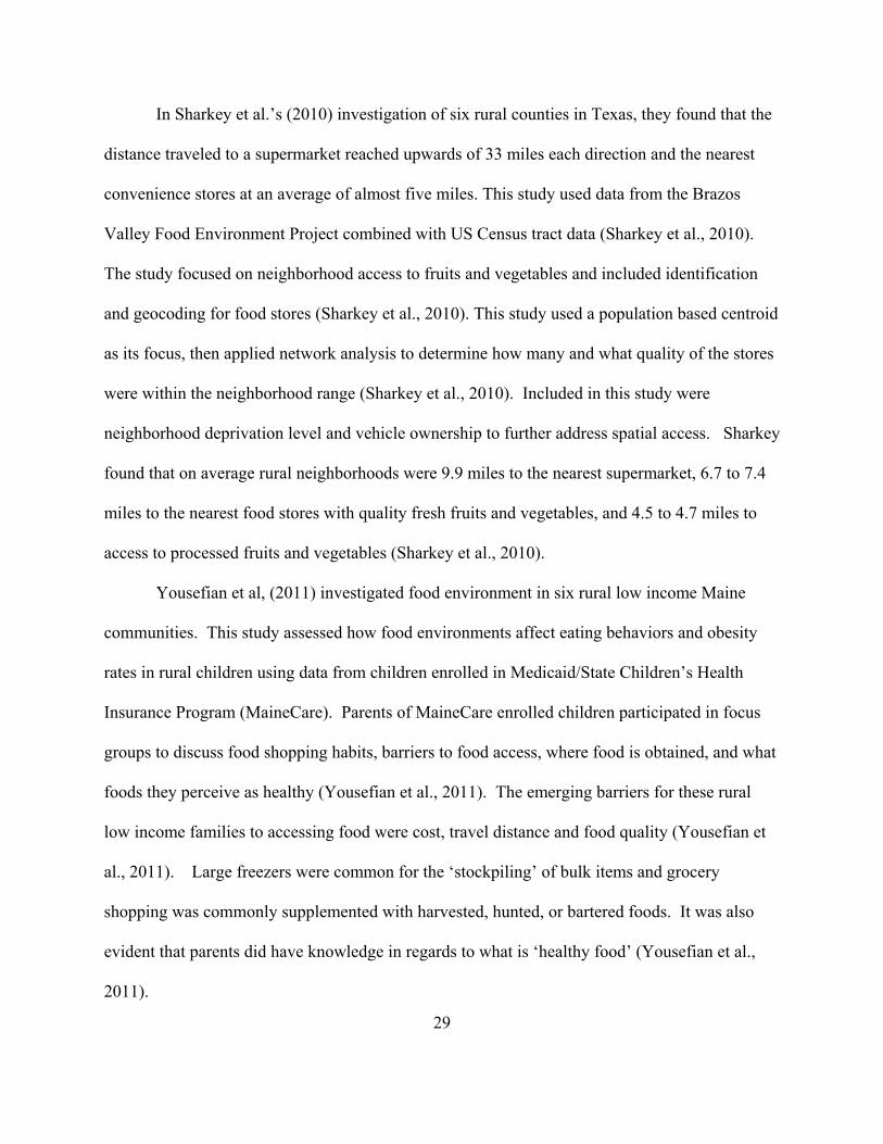
In Sharkey et al.’s (2010) investigation of six rural counties in Texas, they found that the
distance traveled to a supermarket reached upwards of 33 miles each direction and the nearest
convenience stores at an average of almost five miles. This study used data from the Brazos
Valley Food Environment Project combined with US Census tract data (Sharkey et al., 2010).
The study focused on neighborhood access to fruits and vegetables and included identification
and geocoding for food stores (Sharkey et al., 2010). This study used a population based centroid
as its focus, then applied network analysis to determine how many and what quality of the stores
were within the neighborhood range (Sharkey et al., 2010). Included in this study were
neighborhood deprivation level and vehicle ownership to further address spatial access. Sharkey
found that on average rural neighborhoods were 9.9 miles to the nearest supermarket, 6.7 to 7.4
miles to the nearest food stores with quality fresh fruits and vegetables, and 4.5 to 4.7 miles to
access to processed fruits and vegetables (Sharkey et al., 2010).
Yousefian et al, (2011) investigated food environment in six rural low income Maine
communities. This study assessed how food environments affect eating behaviors and obesity
rates in rural children using data from children enrolled in Medicaid/State Children’s Health
Insurance Program (MaineCare). Parents of MaineCare enrolled children participated in focus
groups to discuss food shopping habits, barriers to food access, where food is obtained, and what
foods they perceive as healthy (Yousefian et al., 2011). The emerging barriers for these rural
low income families to accessing food were cost, travel distance and food quality (Yousefian et
al., 2011). Large freezers were common for the ‘stockpiling’ of bulk items and grocery
shopping was commonly supplemented with harvested, hunted, or bartered foods. It was also
evident that parents did have knowledge in regards to what is ‘healthy food’ (Yousefian et al.,
2011).
30
In the rural Maine study it was found that individuals in some communities traveled as
much as 40 miles one way and those people residing in communities nearest to supermarkets
traveled 10 to 15 miles each direction (Yousefian et al., 2011). Lengthy driving distances lead
to fewer trips to larger markets and more cost per trip (Lebel, Pampalon, Hamel, & Theriault,
2009; Yousefian et al., 2011). One must not only contend with the cost of the food purchased
but also the time cost of traveling upwards of 40 miles each way and the expense of gasoline and
transportation wear and tear for such trips (Lebel et al., 2009; Yousefian et al., 2011). These
trips are then supplemented by the purchase of perishables such as dairy and meats at local more
expensive markets and convenience stores (Yousefian et al., 2011). While both of these studies
reflect rural populations, Yousefian et al.’s 2011 study in the state of Maine is more germane to
the study of Appalachian food deserts than is rural Texas based on the topography and
demographics of Maine.
Support for these ‘stockpile’ grocery trips may be seen in Thomas’s article in that food
store type was analyzed with distance to stores, food insecurity, and the type of store chosen
patronized. It was found that only 15% of individuals regularly shop at the closest food outlet to
their homes, and that most drive well beyond to other supermarkets (Thomas, 2010). This was
the case in both food secure and insecure households; however, it was considered that the cost of
travel time is greater for the food insecure (Thomas, 2010). Quality of grocery stores was not
assessed but may play a role in grocery shopping choices. The concern with increased distances
to grocery stores is that access may influence how households manage food insecurity (Thomas,
2010). In a study conducted in nonmetropolitan Michigan, store location competed with food
price, food selection, and food quality, and while distance is more of a concern in the current
31
economic climate, most households still chose to drive farther for better prices and selection
rather than shop at closer small grocery stores (Webber & Rojhani, 2010).
Transportation can become a critical barrier to access to healthy foods for rural residents.
There is limited if any public transportation options, and while these studies showed that the
majority of rural residents at least have access to a car, that does not negate the time and money
expenditures of using those transportation options. Also, access to a car does not equate to car
ownership that may also decrease access opportunities. It must also be considered that there are
members of these rural communities who remain unaccounted for, living unacknowledged
without modern resources that would lead to their identification and representation within the
current US census system (Amberg, 2002).
Time and distance traveled to supermarkets may pose more of a barrier in rural
mountainous regions that often do not have immediate access to interstates. Small state
highways and rural back roads commonly have much lower speed limits and take paths that
follow the geographic topography of the region leading to longer more indirect paths to
destinations. While these road features are often a tourist draw to remote scenic locations, for
those who reside year long in rural Appalachia, it may mean less access to healthy foods. It is
for this reason that addressing time of travel is needed in the identification of rural food deserts
instead of using buffer zone analysis that represents access “as the crow flies”.
Fruit and Vegetable Availability and Intake
Food store type does play a role in fruit and vegetable access. In a Scottish study by
Cummins et al. (2009), spatial analysis was conducted based on the Scottish Urban Rural
Classifications and Index of Multiple Deprivation to address variations in fresh fruit and
32
vegetable quality. This study addressed the differences between urban, small town, and rural as
well as affluent and deprived designations for each population density and reflects a similar
methodology to the USDA analysis for food deserts (Cummins et al., 2009). Individual
consumers were surveyed at each of the markets through a Healthy Eating Indicator Shopping
Basket (HEISB) (Cummins et al., 2009). The HEISB is a survey report consisting of a Likert
scale that replicates the evaluations shoppers commonly make when choosing fresh produce for
purchase and includes evaluations based on a list of commonly purchased fruits and vegetables
(Cummins et al., 2009). A variety of food outlet types in both rural and urban locations were
assessed on food availability and quality (Cummins et al., 2009). It was determined that
medium sized stores that were specifically grocery stores had better quality scores than did large
scale bulk based stores (Cummins et al., 2009). The Scottish study also determined that when a
store sells food secondary to its primary business, the fruit and vegetable quality was lowest
(Cummins et al., 2009).
In Sharkey et al.’s 2010 fruit and vegetable assessment in Texas, convenience stores were
less likely to have fruits and vegetables available than both traditional and nontraditional food
outlets. Nontraditional food stores can include mass merchandisers, pharmacies, and dollar
stores. The nontraditional food markets usually carry processed fruits and vegetables, while
convenience stores are more likely to carry processed vegetables but not processed fruits
(Sharkey et al., 2010). Also the availability of fresh fruits and vegetables was limited, with the
best access at large supermarkets in comparison with all other food store options including
smaller grocery stores (Sharkey et al., 2010). However, one concern is that access to fresh fruits
and vegetables was still limited, and access to fruits and vegetables increased when the definition
of fruits and vegetables was expanded to include processed versions (Sharkey et al., 2010).
33
The best access to fruits and vegetables occurs when there is close proximity and
increased numbers of shopping options (Sharkey et al., 2010). When residents have these shorter
distance options they often have a better variety of and access to fruits and vegetables then they
would by driving to the nearest supermarket (Sharkey et al., 2010). One rural Texas based study
found distance to be inversely associated with fruit and vegetable intake (Dean & Sharkey,
2011). This was particularly the case for rural residents (Dean & Sharkey, 2011). When there is
limited access to fruits and vegetable in high deprivation neighborhoods, distance plays a crucial
role. Fruit and vegetable access is affected by the distance to access points in both rural and
urban settings (Sharkey et al., 2010).
However, results from the Pearson, Russell, Michael, and Barker (2005) United Kingdom
study that used a similar methodology of distance between individual residences and
supermarkets showed that food deserts did not influence fruit and vegetable intake. The Pearson
et al. (2005) study is inconsistent with other studies addressing the effect of food deserts on fruit
and vegetable intake (Larson et al., 2009; Sharkey et al., 2010; Zenk et al., 2005). This
inconsistency is likely due to variations in community selection. Four communities were used,
two urban and two rural, to represent varied population densities (Pearson et al., 2005). Also,
neighborhood deprivation was taken into account to ensure that two of the communities met a
high level of deprivation and the other two met a low level of deprivation (Pearson et al., 2005).
Community deprivation was based on the United Kingdom’s (UK) Index of Multiple
Deprivation scores, which provide a identified deciles and rank (Pearson et al., 2005). However,
both of the urban communities were in the most deprived deciles for socioeconomic deprivation
of English wards, with scores of 55.5 and 51 (rank 374 of 8,414 and 524 of 8,414), while the
rural populations had much less socioeconomic deprivation scores (17.9 [rank 3,996] and 14.9

34
[rank 4,754]) (Pearson et al., 2005). Neighborhood deprivation and socioeconomic status are
used in the identification of healthy food access and availability concerns (Ahern et al., 2011;
Black & Macinko, 2008; Ford & Dzewaltowski, 2011; Pearson et al., 2005; Smith et al., 2010).
By only using affluent rural communities, Pearson et al.’s (2005) study cannot compare
population density in its assessment, when the communities selected do not reflect populations of
similar socioeconomic deprivation.
When combined, distance traveled, fruit and vegetable quality, and fruit and vegetable
variety create a strong barrier that decreases healthy food availability. This is particularly true
for fresh fruits and vegetables that require greater concern in regards to storage and do not
maintain the shelf life of processed fruits and vegetables often available in smaller food outlets.
In future research it will be important to understand how distance affects the type of fruits and
vegetable consumed, not just their overall availability to full understand healthy food access
issues.
Spatial Analysis
The articles related to spatial analysis of food availability that were reviewed for this
research needed to meet the following criteria: all studies must include a spatial analysis
component for analysis of food environment, access, availability, and/or food desert
identification; and all of the studies must include analysis of rural regions either exclusively or in
comparison with urban areas. Articles were found through academic search engines using the
following terms: “food desert ”, “ food access”, and “food availability” alone or in conjunction
with the following terms: “spatial analysis”, “GIS”, “mapping”, and “rural”. The searches were
limited to human subjects and those papers available in English. Date was not included in the
35
initial limitations. Due to the modernity of the technology used for food desert mapping, articles
were no more than 15 years old.
Of the articles reviewed, seven were U.S. based studies, two were from New Zealand,
and two were from the UK. Three of the US studies used North American Industry
Classification System (NAICS) 44511 or 445110 coded data (Super market or other grocery
stores, not including convenience stores) for their studies to assess food access (Blanchard &
Lyson, 2002; McEntee & Agyeman, 2009; Schafft et al., 2009). An additional US based study
by Liese, Weis, Delores, Smith, and Lawson, (2007) used a similar state managed data set for
identifying markets (Licensed Food Service Facility Database) in South Carolina. Of the 11
studies reviewed, 3 investigated rural food desert analysis exclusively while the other 8 were
comparative studies of urban and rural food deserts.
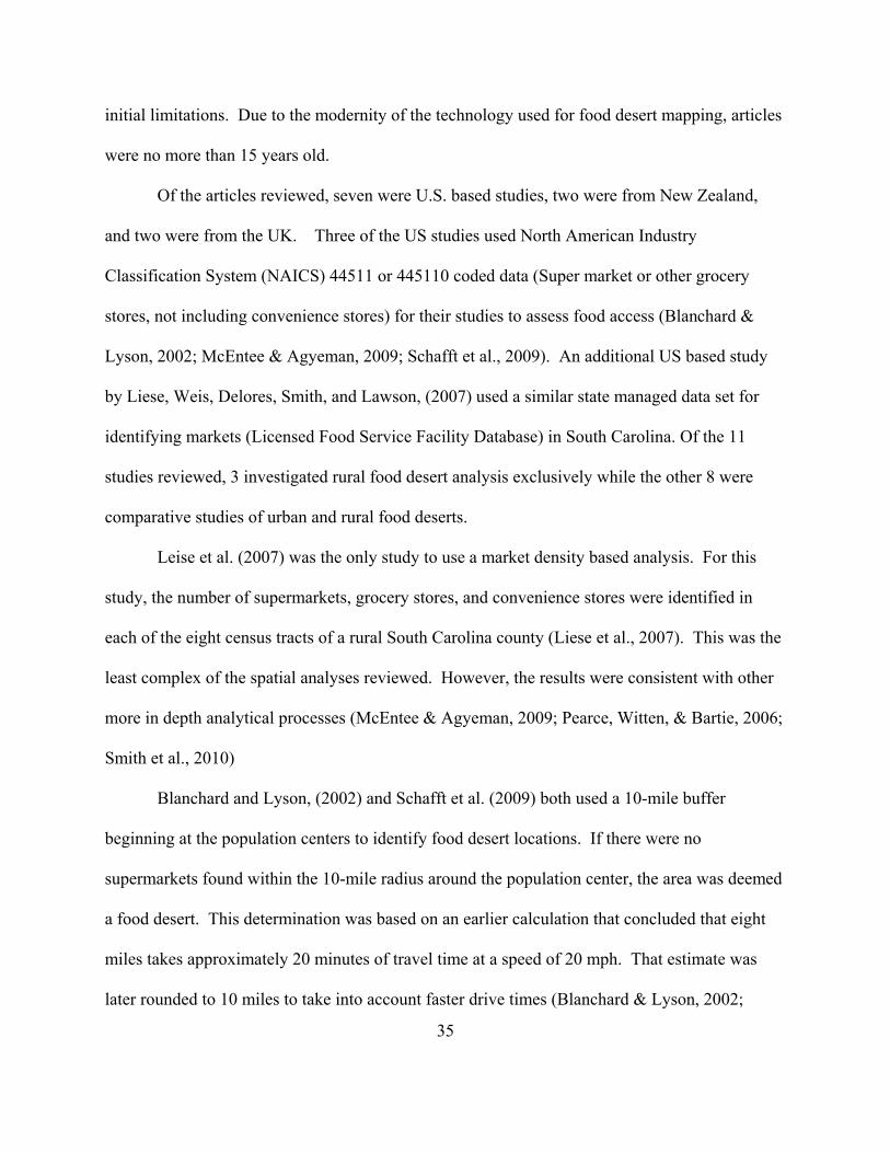
Leise et al. (2007) was the only study to use a market density based analysis. For this
study, the number of supermarkets, grocery stores, and convenience stores were identified in
each of the eight census tracts of a rural South Carolina county (Liese et al., 2007). This was the
least complex of the spatial analyses reviewed. However, the results were consistent with other
more in depth analytical processes (McEntee & Agyeman, 2009; Pearce, Witten, & Bartie, 2006;
Smith et al., 2010)
Blanchard and Lyson, (2002) and Schafft et al. (2009) both used a 10-mile buffer
beginning at the population centers to identify food desert locations. If there were no
supermarkets found within the 10-mile radius around the population center, the area was deemed
a food desert. This determination was based on an earlier calculation that concluded that eight
miles takes approximately 20 minutes of travel time at a speed of 20 mph. That estimate was
later rounded to 10 miles to take into account faster drive times (Blanchard & Lyson, 2002;
36
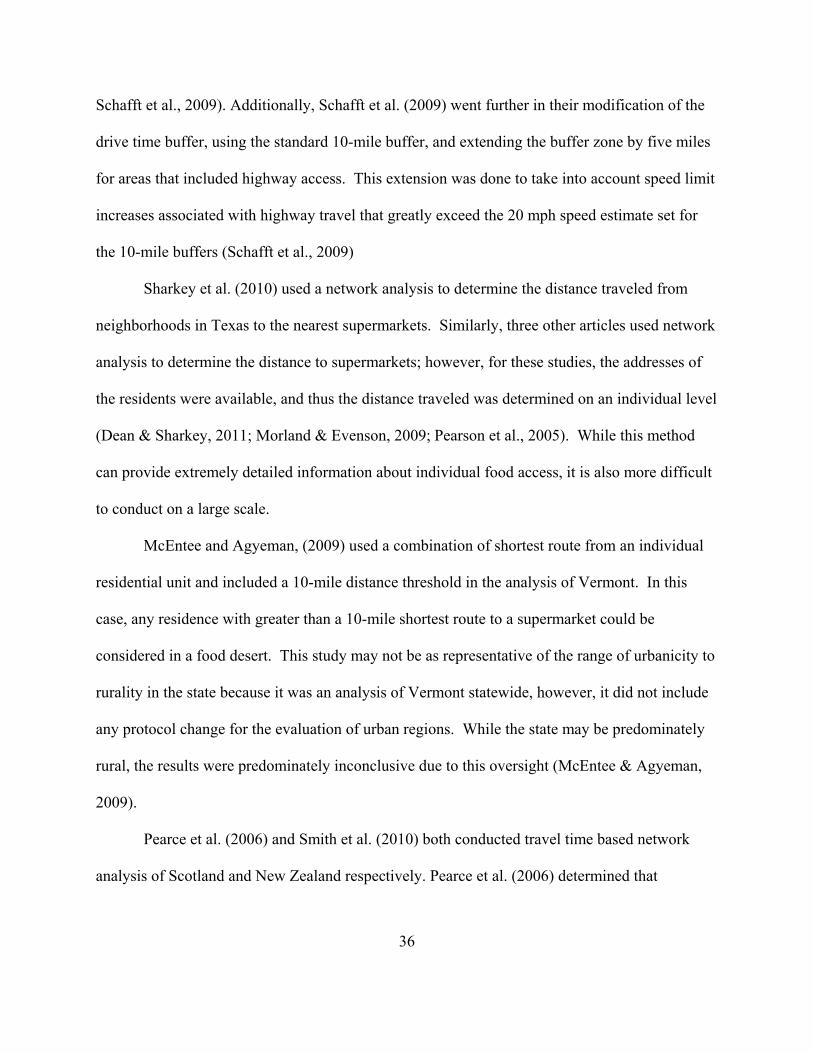
Schafft et al., 2009). Additionally, Schafft et al. (2009) went further in their modification of the
drive time buffer, using the standard 10-mile buffer, and extending the buffer zone by five miles
for areas that included highway access. This extension was done to take into account speed limit
increases associated with highway travel that greatly exceed the 20 mph speed estimate set for
the 10-mile buffers (Schafft et al., 2009)
Sharkey et al. (2010) used a network analysis to determine the distance traveled from
neighborhoods in Texas to the nearest supermarkets. Similarly, three other articles used network
analysis to determine the distance to supermarkets; however, for these studies, the addresses of
the residents were available, and thus the distance traveled was determined on an individual level
(Dean & Sharkey, 2011; Morland & Evenson, 2009; Pearson et al., 2005). While this method
can provide extremely detailed information about individual food access, it is also more difficult
to conduct on a large scale.
McEntee and Agyeman, (2009) used a combination of shortest route from an individual
residential unit and included a 10-mile distance threshold in the analysis of Vermont. In this
case, any residence with greater than a 10-mile shortest route to a supermarket could be
considered in a food desert. This study may not be as representative of the range of urbanicity to
rurality in the state because it was an analysis of Vermont statewide, however, it did not include
any protocol change for the evaluation of urban regions. While the state may be predominately
rural, the results were predominately inconclusive due to this oversight (McEntee & Agyeman,
2009).
Pearce et al. (2006) and Smith et al. (2010) both conducted travel time based network
analysis of Scotland and New Zealand respectively. Pearce et al. (2006) determined that
37
geographic variation can affect accessibility and that the use of travel time may provide for more
precision in future research in food environment analysis.
A wide range of methodologies have been used to operationally define food deserts and
relate their impact on food access. All of the reviewed studies used methods based on evaluating
locations of supermarkets in relationship to residences. While several studies used a population
center to define residences, this may not be as accurate for representing rural areas where
population density is sparse (Blanchard & Lyson, 2002; Smith et al., 2010). It creates a situation
where not all areas of a population designation are represented by the analysis. For this reason it
seems to in the best interest of analysis to use the market locations as the central evaluative focus
as used (McEntee & Agyeman, 2009; Pearce et al., 2006). By starting at the supermarket and
expanding outward, the spatial analysis would reflect what the scope of impact of the grocery
store is, not the population center.
Because it has been acknowledged that geographic variation can play an important role in
food access, this is a factor that must be taken into account. By using a travel-time based
analysis, issues of geographical features that impede efficient travel would be addressed. This is
particularly important when evaluating a region that has a mountainous terrain and therefore
travel systems that can be less than efficient. A network analysis with a central point of a market
that uses time traveled based on the available research (20 minute one direction) could identify
areas with similar vulnerabilities that would otherwise not be brought to attention.
Conclusion
The strong association between food access and health outcomes drives the need for
further research on food availability among vulnerable populations. It is imperative that in the
38
analysis of food deserts, topographical geography and neighborhood deprivation be taken into
account. These are leading indicators of poor healthy food access and availability. The current
methods for identifying these food deserts represent population dense and geographically
moderate regions well; however, the current systems do not take into account the significance of
many rural access issues. From a public health context, this leaves vulnerable populations
unidentified and without the aid needed to improve their overall health. Without the
identification of populations at-risk, there is no proof of need for policy and food environment
access changes to improve rural community access to healthy foods. In an area such as the
Appalachian region, that has double the percent of rural residents when compared to the US as a
whole, and represents a population of great economic distress, it is crucial to justly represent the
population’s food access needs (Appalachian Regional Commission, 2012).
39
CHAPTER 3
METHODS
Data Used
The data for this research were collected from multiple sources. Image files for use in
GIS analysis included state basemaps, county and census tract boundary images, and core based
statistical areas for micropolian and metropolitan region gathered from the US Census (US
Census Burearu, Geography Division, 2011). Rural Urban Commuting Area (RUCA) codes for
the county level were obtained from the United States Department of Agriculture (USDA)
(USDA, 2004). Also collected from the US Census were American Community Survey (ACS) 5-
year census tract level estimates for poverty and income levels for the selected Appalachian
census tracts to determine low income status (US Census Bureau: American FactFinder, 2012;
USDA: Economic Research Services, 2011). Five-year median household income and poverty
rate estimate data were used to ensure that the most comprehensive representation of
Appalachian Region census tracts, as both 1- and 3-year estimates were missing data from
several Appalachian Region census tracts (US Census Bureau: American FactFinder, 2012).
Roadway locations and attributes were obtained from the US Census topographically integrated
geographic encoding and referencing system (TIGER), and the North Carolina Department of
Transportation (NCDOT) (NCDOT: GIS Unit, 2012; US Census Burearu, Geography Division,
2011). Further attribute data on speed limits were collected from the North Carolina, Kentucky,
and Tennessee Departments of Transportation (Kentucky State Legislature, 2007; NCDOT: GIS
Unit, 2012; Tennessee State Legislature, 2012). Economic distress designation, Appalachian
county, and subregion designations were collected from the Appalachian Regional
40
Commission’s data resources (Appalachian Regional Commission, 2012). Supermarket
locations were acquired from Hoover’s (Hoover's, 2012). All supermarkets that met the criteria
of a large grocery store or chain supermarket were included, while convenience stores were not
included. These types of sites were coded with the primary NAICS code of 445110 (USDA:
Economic Research Services, 2011). As per USDA methods for supermarket selection, these
stores were then limited to those with a revenue of two million dollars or more in the past fiscal
year (USDA: Economic Research Services, 2011). Also in following the USDA methods, the
stores were cross referenced with available state Women, Infant Child (WIC) supplemental
program lists, eliminating any store that was not a WIC vendor (USDA: Economic Research
Services, 2011). Health outcomes data for comparative analysis were collected from the Center
for Disease Control and Prevention’s (CDC’s) National Diabetes Surveillance System (NDSS)
(Centers for Disease Control and Prevention: National Diabetes Surveillance System, 2011).
These data included 3-year, county level prevalence estimates for diagnosed diabetes and obesity
(Centers for Disease Control and Prevention: National Diabetes Surveillance System, 2011).
Sample Selection
Why Appalachia?
The Appalachian region is defined as the region that follows the “spine” of the
Appalachian Mountains from northern Mississippi to southern New York (Appalachian Regional
Commission, 2012). This covers a 205,000 square mile region that encompasses all of West
Virginia and parts of 12 other states including eastern Tennessee, western North Carolina, and
eastern Kentucky (Appalachian Regional Commission, 2012). Rural residents make up 42% of
41
the region’s population more than double the national percentage of rural residents (Appalachian
Regional Commission, 2012).
The criteria for area selection for this research required that the county be a contiguous
part of the Appalachian Region of Tennessee, North Carolina, or Kentucky. These states were
selected based the fact that they contain counties that represent the Appalachian Regional
Commission subregion designations of Central and South Central Appalachia. Appalachian
subregions are contiguous regions of Appalachia that were considered by the Appalachian
Regional Commission to have relatively homogeneous characteristics (including demographics,
economics and topography) (Appalachian Regional Commission, 2012). These subregions were
revised and further divided in 2009 to reflect current economic and transportation data available
for the Region (Appalachian Regional Commission, 2012). The use of North Carolina,
Tennessee, and Kentucky was based on the decision to use Tennessee as the basis for this
research. Tennessee was used for this research to cumulatively represent the rural and regional
aspects of my academic body of work developed over the course of my tenure in the Community
and Behavioral Health Department of the College of Public Health at East Tennessee State
University. Because Tennessee represents both the Central and South Central subregions of the
Appalachian Region, it was decided to use other states that represent those subregions, Kentucky
representing the Central subregion and North Carolina representing the South Central subregion.
Regional Economics
Historically the Appalachian Region has been considered an area of economic
disadvantage, with a 33% poverty rate in 1965 (Appalachian Regional Commission, 2012).
While this rate had declined to 18% in 2008, it still maintains a much higher number of high
poverty counties than the US average (13.8%) and with the current state of the US economy, are
42
at a greater risk of economic disadvantage (Appalachian Regional Commission, 2012). While
progress has been made to improve the economic environment of Appalachia, the region still
struggles, not maintaining the same economic stability as the rest of the US (Appalachian
Regional Commission, 2012). This is most evident in the Central region where economic
distress is apparent in the concentrated areas of poor health, high poverty, educational disparities,
and unemployment (Appalachian Regional Commission, 2012).
Economic Distress
Economic distress is measured by the Appalachian Regional Commission using an index
based county economic classification system referred to as the National Index Value (NIV) rank
(Appalachian Regional Commission, 2012). This system is used to identify and monitor
Appalachian counties’ economic status using the county level averages for three economic
indicators: 3-year average unemployment rate, per capita market income, and poverty rate
compared with the national averages (Appalachian Regional Commission, 2012). Counties are
then designated as distressed, at-risk, transitional, competitive, or attainment (Appalachian
Regional Commission, 2012). A distressed county is described as ranking in the worst 10% by
the NIV rank of all US counties (Appalachian Regional Commission, 2012). At-risk counties
fall within the worst 10% to 25% NIV rank of US counties (Appalachian Regional Commission,
2012). Transitional designated counties can include any county ranked between the 25% worst
and 25% best US counties (Appalachian Regional Commission, 2012). For competitive
designations, counties must have an NIV rank of the best 10% to 25%, with attainment
designated counties being ranked within the best 10% (Appalachian Regional Commission,
2012).
43
Often there are significant portions of counties that may not be ranked as distressed
counties yet may have distressed characteristics. These are census tracts within at-risk and
transitional counties with a median family income of less than or equal to 67% of the US
average, and a poverty rate equal to or greater than 150% of the US average (Appalachian
Regional Commission, 2012). These economically distressed census tracts are referred to as
distressed areas (Appalachian Regional Commission, 2012).
The Appalachian region survives with an elevated level of economic distress. The
Appalachian region of Kentucky alone contains 41 economically distressed counties and 9
economically at-risk counties (Appalachian Regional Commission, 2011a). The remaining 4
counties are considered economically transitional, but all contain census tracts designated as
distressed areas (Appalachian Regional Commission, 2011a). With 1 distressed and 10 at-risk
counties, the Appalachian region of North Carolina, has the lowest rate of distressed county
rankings (Appalachian Regional Commission, 2011b). However, all of these counties have
distressed areas within them, and of the 18 transitional counties in North Carolina, half contain
economically distressed areas (Appalachian Regional Commission, 2011b). There are 17
economically distressed counties and 18 economically at-risk counties in the Appalachian region
of Tennessee (Appalachian Regional Commission, 2011c). Of these at-risk counties, 15 have
distressed areas, and of the 16 transitional counties, 12 contain distressed areas (Appalachian
Regional Commission, 2011c). It is evident that even with some variation in economic distress
between these three states, all maintain elevated designations of economic distress at the county
or census tract level. No Appalachian county in any of these three states is considered
competitive or at attainment. Economic burden and distress are features still defining the
44
Appalachian Region, and with the current economic climate, these areas must cope with more
economic risk than other regions of their respective states.
It is apparent when comparing the economic status for 2012 with the 2008 economic
status, that there is a discrepancy. There has been an obvious decline in the number of
transitional counties within the Kentucky, North Carolina, and Tennessee Appalachian Regions,
and there are no longer any counties designated as competitive. This transition mirrors the
current US and world economic trend. So, while there have been improvements with regard to
economic status because the inception of the Appalachian Regional Commission in the mid 60s,
more recently a decline can be seen.
Rural Urban Commuting Area Codes
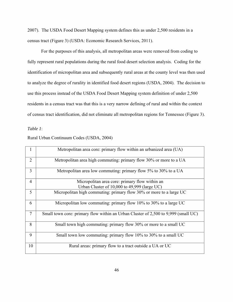
Selected areas were required to be either rural or micropolitan regions. Rural urban
commuting area (RUCA) codes at the census tract level were used to eliminate all tracts that are
in metropolitan regions. Census tracts within micropolitan regions were included as rural
because they are representative of core based statistical areas for rural commuting (Table 1;
Figure 2.1) (USDA: Economic Research Services, 2011) and may be a primary resource
for supermarket and grocery store access for rural communities.
Rural urban commuting area codes are a common tool for measuring rurality. There are
two ways of observing the comparisons of urban and rural. Sometimes rural is considered a
variable that is lacking urbanism; however, rural areas are unique in nature with their own
distinguishing features and issues (Hall, Kaufman, & Ricketts, 2006). The delineation of rurality
that is used by the USDA was developed by the White House’s Office of Management and
Budget (OMB) and addresses rurality at the level of census tract (USDA: Economic Research
45
Services, 2011). It addresses the issue of whether there is a “central core” associated with the
county either by proximity or commuter status. Currently the classification contains 10 primary
codes (Table 1) (USDA: Economic Research Services, 2011). For research and policy
applications, however, the full code sets are not readily used, instead the system allows for the
selection of code combinations that can meet a variety of analysis needs, most commonly, codes
1 through 3 are considered metropolitan, 4 through 6 are micropolitan, and 7 through 10 are rural
(Table 1; Figure 2) (USDA: Economic Research Services, 2011).
Currently within this coding system, the regions that are designated as micropolitan and
metropolitan are considered core based statistical areas (CBSAs), while those not designated as
such are considered outside CBSAs, or non CBSAs (Figure 2) (Hall et al., 2006). Some
researchers may have a tendency to combine the metropolitan and micropolitan areas because
they are both considered CBSAs, but this may not be an ideal option considering that
micropolitan areas may have rural characteristics (Hall et al., 2006; Slifkin, Randolph, &
Ricketts, 2004). This methodology is often used because urban regions often have an area of
influence that extends well beyond their defined tract borders (USDA: Economic Research
Services, 2011). Another way to combine the regions is to designate that all regions that are not
metropolitan areas are rural. While this analytic plan will expand the rural areas it may not
accurately represent micropolitan regions that are CBSAs (Hall et al., 2006).
USDA uses standards for identifying rural areas based upon the RUCA system that
includes defining metropolitan and micropolitan areas (Table 1). The USDA has expanded the
definition of urban to include micropolitan and small town centers (USDA, 2007). This shift
narrows the definition of rural areas to those under 2,500 residents in an area (Figure 3) (USDA,
46
2007). The USDA Food Desert Mapping system defines this as under 2,500 residents in a
census tract (Figure 3) (USDA: Economic Research Services, 2011).
For the purposes of this analysis, all metropolitan areas were removed from coding to
fully represent rural populations during the rural food desert selection analysis. Coding for the
identification of micropolitan area and subsequently rural areas at the county level was then used
to analyze the degree of rurality in identified food desert regions (USDA, 2004). The decision to
use this process instead of the USDA Food Desert Mapping system definition of under 2,500
residents in a census tract was that this is a very narrow defining of rural and within the context
of census tract identification, did not eliminate all metropolitan regions for Tennessee (Figure 3).
Table 1:
Rural Urban Continuum Codes (USDA, 2004)
1 Metropolitan area core: primary flow within an urbanized area (UA)
2 Metropolitan area high commuting: primary flow 30% or more to a UA
3 Metropolitan area low commuting: primary flow 5% to 30% to a UA
4 Micropolitan area core: primary flow within an Urban Cluster of 10,000 to 49,999 (large UC)
5 Micropolitan high commuting: primary flow 30% or more to a large UC
6 Micropolitan low commuting: primary flow 10% to 30% to a large UC
7 Small town core: primary flow within an Urban Cluster of 2,500 to 9,999 (small UC)
8 Small town high commuting: primary flow 30% or more to a small UC
9 Small town low commuting: primary flow 10% to 30% to a small UC
10 Rural areas: primary flow to a tract outside a UA or UC
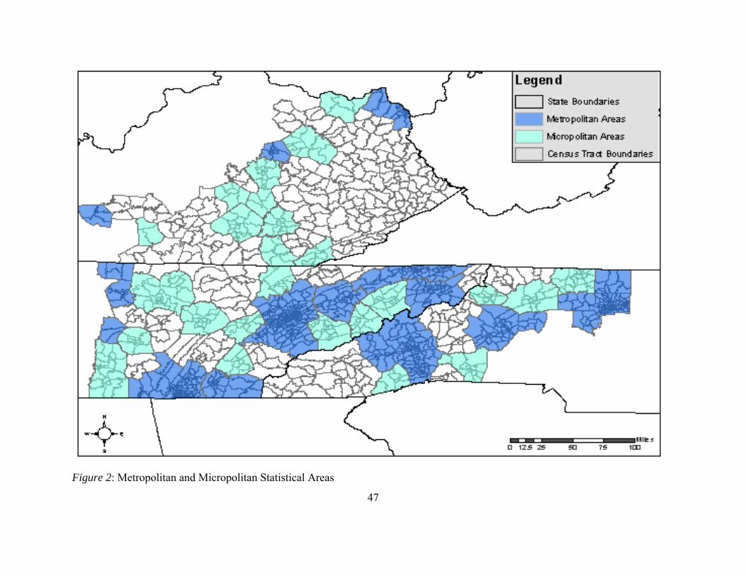
47
Figure 2: Metropolitan and Micropolitan Statistical Areas
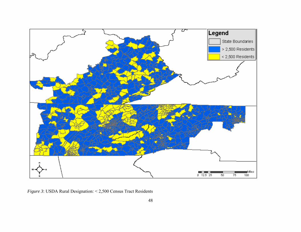
48
Figure 3: USDA Rural Designation: < 2,500 Census Tract Residents
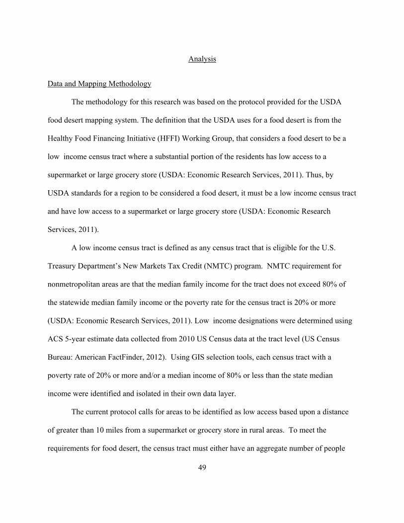
49
Analysis
Data and Mapping Methodology
The methodology for this research was based on the protocol provided for the USDA
food desert mapping system. The definition that the USDA uses for a food desert is from the
Healthy Food Financing Initiative (HFFI) Working Group, that considers a food desert to be a
low income census tract where a substantial portion of the residents has low access to a
supermarket or large grocery store (USDA: Economic Research Services, 2011). Thus, by
USDA standards for a region to be considered a food desert, it must be a low income census tract
and have low access to a supermarket or large grocery store (USDA: Economic Research
Services, 2011).
A low income census tract is defined as any census tract that is eligible for the U.S.
Treasury Department’s New Markets Tax Credit (NMTC) program. NMTC requirement for
nonmetropolitan areas are that the median family income for the tract does not exceed 80% of
the statewide median family income or the poverty rate for the census tract is 20% or more
(USDA: Economic Research Services, 2011). Low income designations were determined using
ACS 5-year estimate data collected from 2010 US Census data at the tract level (US Census
Bureau: American FactFinder, 2012). Using GIS selection tools, each census tract with a
poverty rate of 20% or more and/or a median income of 80% or less than the state median
income were identified and isolated in their own data layer.
The current protocol calls for areas to be identified as low access based upon a distance
of greater than 10 miles from a supermarket or grocery store in rural areas. To meet the
requirements for food desert, the census tract must either have an aggregate number of people
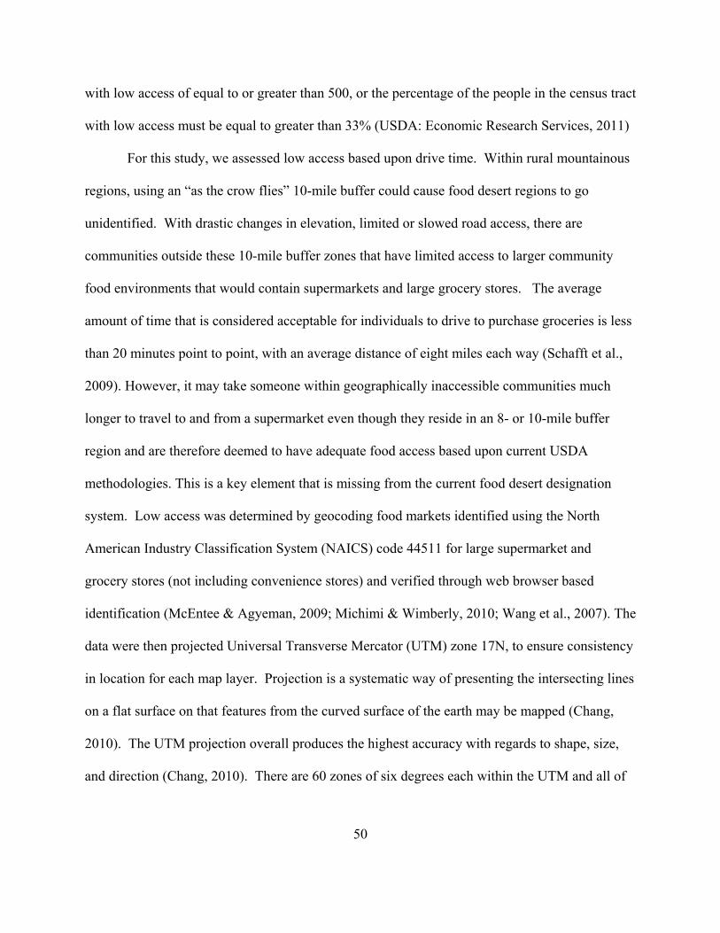
50
with low access of equal to or greater than 500, or the percentage of the people in the census tract
with low access must be equal to greater than 33% (USDA: Economic Research Services, 2011)
For this study, we assessed low access based upon drive time. Within rural mountainous
regions, using an “as the crow flies” 10-mile buffer could cause food desert regions to go
unidentified. With drastic changes in elevation, limited or slowed road access, there are
communities outside these 10-mile buffer zones that have limited access to larger community
food environments that would contain supermarkets and large grocery stores. The average
amount of time that is considered acceptable for individuals to drive to purchase groceries is less
than 20 minutes point to point, with an average distance of eight miles each way (Schafft et al.,
2009). However, it may take someone within geographically inaccessible communities much
longer to travel to and from a supermarket even though they reside in an 8- or 10-mile buffer
region and are therefore deemed to have adequate food access based upon current USDA
methodologies. This is a key element that is missing from the current food desert designation
system. Low access was determined by geocoding food markets identified using the North
American Industry Classification System (NAICS) code 44511 for large supermarket and
grocery stores (not including convenience stores) and verified through web browser based
identification (McEntee & Agyeman, 2009; Michimi & Wimberly, 2010; Wang et al., 2007). The
data were then projected Universal Transverse Mercator (UTM) zone 17N, to ensure consistency
in location for each map layer. Projection is a systematic way of presenting the intersecting lines
on a flat surface on that features from the curved surface of the earth may be mapped (Chang,
2010). The UTM projection overall produces the highest accuracy with regards to shape, size,
and direction (Chang, 2010). There are 60 zones of six degrees each within the UTM and all of
51
the Appalachian region of Kentucky, Tennessee, and North Carolina reside within zone 17 north
(Chang, 2010).
The speed limit for each road type was established using department of transportation
data from each state (Kentucky State Legislature, 2007; NCDOT: GIS Unit, 2012; Tennessee
State Legislature, 2012). Drive time in minutes for each measured road section was then
calculated by dividing the road segment distance in meters by the speed limit converted from
miles per hour to meters per minute. A network analysis was created to include a travel time of
20 minutes based on road data collected from the US Census TIGER and the Kentucky, North
Carolina, and Tennessee Departments of Transportation (Kentucky State Legislature, 2007;
NCDOT: GIS Unit, 2012; Pearce et al., 2006; Tennessee State Legislature, 2012; US Census
Burearu, Geography Division, 2011). The network analysis assembled driving paths composed
of road segment drive time measures extending from each geolocated grocery store and
supermarket for a 20 minute length. All spatial analyses were performed using by ESRIs arcGIS
101.
Once mapping was completed, the surface area was compared with an overlay of the
USDA food desert identification for the selected region to determine reproducibility of the
modeling with USDA methodology and to determine if any of the USDA food desert regions
expanded. The maps were also visually inspected for any new areas that may have been
identified as food deserts due to the modified methodology of drive time network analysis.
Statistical variations in the areas of the two food desert methodology results were determined
through multivariate regression analysis.
1 Copyright © 1995–2012 Esri. All rights reserved. Published in the United States of America.
52
Statistical Analysis
This study is a cross sectional study of grocery store access areas in low income rural
Appalachia. The data collected were used to compare both identified food desert results based
on methodology variations between the USDA and modified models as well as associated health
outcomes for both areas. This was accomplished through spatial and statistical analysis of the
resulting food desert regions.
Frequency and statistical significance were performed using SAS® software2 by state,
food desert method, economic designation, health outcomes (diabetes and obesity), and county
RUCA code designation. Due to low sample size the chi square analysis used initially was not
used, instead a Fisher’s Exact Test was performed.
A regression analysis was performed for diabetes and obesity within both food desert
models for univariate analysis and multivariate analysis controlling for RUCA designation and
economic designation. Further univariate analysis was run to assess the relationship between the
health outcomes and RUCA designation and economic designation. All regression analysis was
run using proc logistic model in SAS ® software2.
Dependent Variables
Those counties that have census tracts within them identified as food desert regions by
each of the two mapping methods were compared based upon county level health outcomes
(obesity and diabetes). Diabetes and obesity are both nutrition related conditions that have been
examined in relation to food deserts. With literature supporting both obesity and diabetes as
2 SAS and all other SAS Institute Inc. product or service names are registered trademarks or trademarks of SAS
Institute Inc. in the USA and other countries. ® indicates USA registration.
53
being linked to the presence of food deserts, these health outcomes were used as a comparison
for determining if the modified model identified populations with similar health risk rates to
those identified by the USDA methods (Ahern et al., 2011; Babey et al., 2008).
Dependent variables included categorical county level statistical estimates for diabetes
and obesity from the National Diabetes Surveillance System (Centers for Disease Control and
Prevention: National Diabetes Surveillance System, 2011). These data were derived using US
census population data and results from the Behavioral Risk Factor Surveillance Survey
(BRFSS) (Centers for Disease Control and Prevention: National Diabetes Surveillance System,
2011). These estimates were based upon 3 years of data (2006, 2007, 2008) to improve the
precision of the year specific, county level data for diagnosed diabetes and obesity (Centers for
Disease Control and Prevention: National Diabetes Surveillance System, 2011). These estimates
were age adjusted for prevalence and included adult populations of greater than or equal to
twenty years old (Centers for Disease Control and Prevention: National Diabetes Surveillance
System, 2011).
Categorical obesity rates were collected from BRFSS self-reported height and weight and
BMI was then determined (weight in kg/ [height in meters]2) (Centers for Disease Control and
Prevention: National Diabetes Surveillance System, 2011). Individuals were considered obese if
they had a BMI of 30 or greater (Centers for Disease Control and Prevention: National Diabetes
Surveillance System, 2011). Categories were predetermined by the Centers for Disease Control
and Prevention’s National Diabetes Surveillance System (Centers for Disease Control and
Prevention: National Diabetes Surveillance System, 2011). For obesity these categories were the
percent of the county population that was obese: category 0: 0% to 21.9%, category 1: 22.0% to
54
26.2%, category 2: 26.3% to 29.7%, category 3: >=29.8% (Centers for Disease Control and
Prevention: National Diabetes Surveillance System, 2011).
Categorical diabetes rates were collected from BRFSS self-reported questionnaire
response of ‘yes’ to whether they have been diagnosed by a doctor with diabetes (Centers for
Disease Control and Prevention: National Diabetes Surveillance System, 2011). Categories were
predetermined by the Centers for Disease Control and Prevention’s National Diabetes
Surveillance System (Centers for Disease Control and Prevention: National Diabetes
Surveillance System, 2011). These categories were the percent of the county population that had
been diagnosed with diabetes: category 0: 0% to 6.3%, category 1: 6.4% to 7.5%, category 2:
7.6% to 8.8%, category 3: 8.9% to 10.5%, category 4: >= 10.6% (Centers for Disease Control
and Prevention: National Diabetes Surveillance System, 2011).
Independent Variables
Independent variables included food desert methods that were comprised of a
dichotomous designation of counties containing food deserts that were identified using either the
USDA methodology or the modified methodology (USDA, 2004). Covariates included
economic distress designation and RUCA codes both at the county level. ARC’s economic
distress designations for transitional, at-risk and distressed counties were controlled for
(Appalachian Regional Commission, 2012). RUCA county level coding for metropolitan,
micropolitan and rural was also controlled for (USDA, 2004).
Age was not controlled for because the health outcomes were age adjusted to 20 years
age and older (Centers for Disease Control and Prevention: National Diabetes Surveillance
System, 2011). Health outcomes estimates were not available based upon gender, excluding

55
gender from the analysis. Ethnicity was not controlled for because over 95% of the residents
were identified as white by the US census (US Census Bureau: American FactFinder, 2012).
56
CHAPTER 4
RESULTS
Descriptive Data
More counties were designated as food desert by the modified food desert assessment
when compared to the USDA methodology. It is apparent that there is an underrepresentation of
food deserts with the USDA system in where a 10-mile buffer zone is used as opposed to a
network analysis based on driving time. Of the counties designated as micropolitan or rural, 20
counties were found to have USDA food desert census tracts within them, while the modified
assessment produced 65 counties over the three states that contained food deserts (Table 2, Table
3). When compared, only 12 of the USDA’s identified counties were also found by the modified
methodology (Table 2). Of the eight counties that contained food deserts only identified by the
USDA method, four were identified by RUCA coding to be in metropolitan counties (Table 3),
and another four others identified after the fact as not meeting the USDA’s criteria for low
income status of a median income of less than or equal to 80% of the state’s median income or a
poverty level of greater than or equal to 20%, when assessed using ACS 5-year estimates for
poverty and income (US Census Bureau: American FactFinder, 2012; US Census Burearu,
Geography Division, 2011; USDA, 2004; USDA: Economic Research Services, 2011). These
outliers from the recreated methods mean that the selection of census tracts as food desert
regions may not be perfectly reproducible, thus preventing a 100% match of USDA census tract
counties identified by the modified methods as expected. This leads to concerns about the
overall ability, using the provided USDA standards if researchers cannot replicate their results.
57
The distribution of food desert counties throughout the three states of Kentucky, North
Carolina, and Tennessee showed an overall distribution of 33, 17, and 23 counties respectively
(Table 2). The USDA system identifies eight counties in Kentucky, five in North Carolina, and
seven in Tennessee (Figure 4, Table 2, and Table 3). The modified system identified 30
Kentucky, 15 North Carolina, and 21 Tennessee counties (Figure 5). The distribution of food
deserts among the three states was consistent over both methods. When assessed for economic
distress, 37 counties were identified as distressed, 10 as at-risk, and 6 transitional by the
modified methods (Table 3). In identifying the severity of rurality, the modified methods
produced 14 micropolitan counties, 39 rural counties, and no metropolitan counties (Table 3).
There is a visual difference in the size of food desert regions when comparing the USDA
methods to the modified food desert analysis. There are much larger areas of each state
represented by the modified analysis methods (Figure 4, Figure 5). Due to the small sample
size, no significant relationships were identified for the Fischer’s exact test
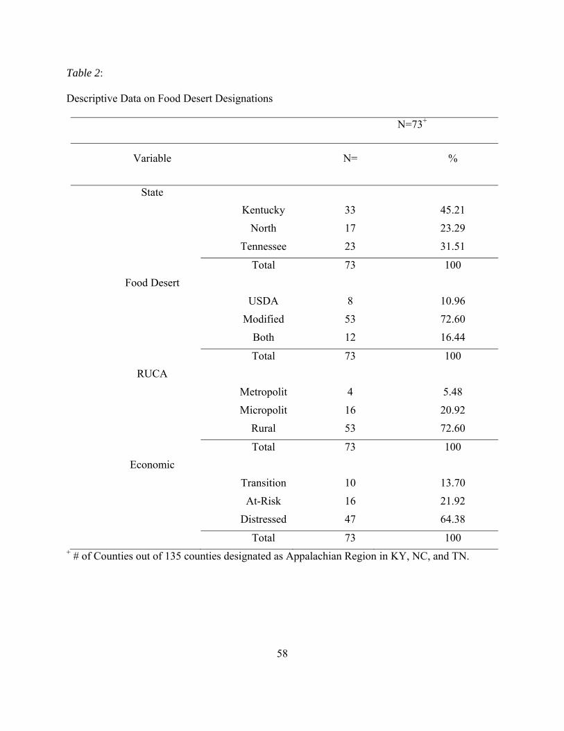
58
Table 2:
Descriptive Data on Food Desert Designations
N=73+
Variable N= %
State Kentucky 33 45.21 North 17 23.29
Tennessee 23 31.51
Total 73 100 Food Desert
USDA 8 10.96 Modified 53 72.60 Both 12 16.44
Total 73 100 RUCA
Metropolit 4 5.48
Micropolit 16 20.92 Rural 53 72.60
Total 73 100 Economic
Transition 10 13.70 At-Risk 16 21.92
Distressed 47 64.38
Total 73 100 + # of Counties out of 135 counties designated as Appalachian Region in KY, NC, and TN.
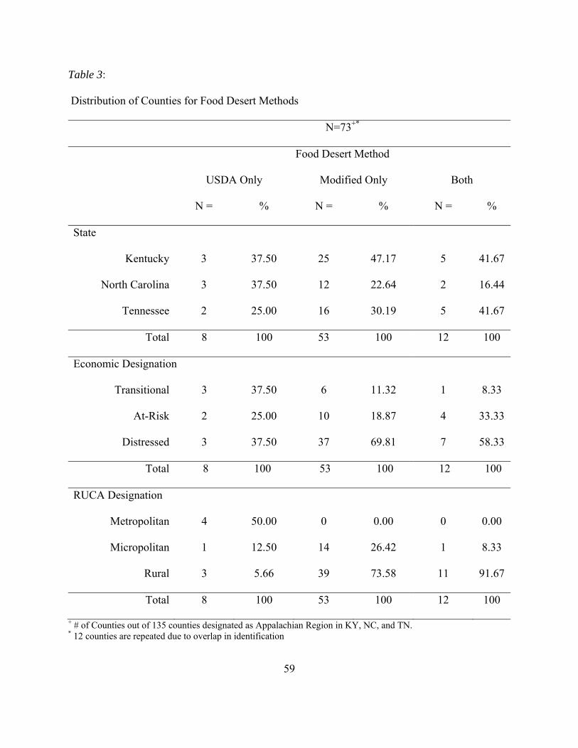
59
Table 3:
Distribution of Counties for Food Desert Methods
N=73+*
Food Desert Method
USDA Only Modified Only Both
N = % N = % N = %
State
Kentucky 3 37.50 25 47.17 5 41.67
North Carolina 3 37.50 12 22.64 2 16.44
Tennessee 2 25.00 16 30.19 5 41.67
Total 8 100 53 100 12 100
Economic Designation
Transitional 3 37.50 6 11.32 1 8.33
At-Risk 2 25.00 10 18.87 4 33.33
Distressed 3 37.50 37 69.81 7 58.33
Total 8 100 53 100 12 100
RUCA Designation
Metropolitan 4 50.00 0 0.00 0 0.00
Micropolitan 1 12.50 14 26.42 1 8.33
Rural 3 5.66 39 73.58 11 91.67
Total 8 100 53 100 12 100
+ # of Counties out of 135 counties designated as Appalachian Region in KY, NC, and TN. * 12 counties are repeated due to overlap in identification
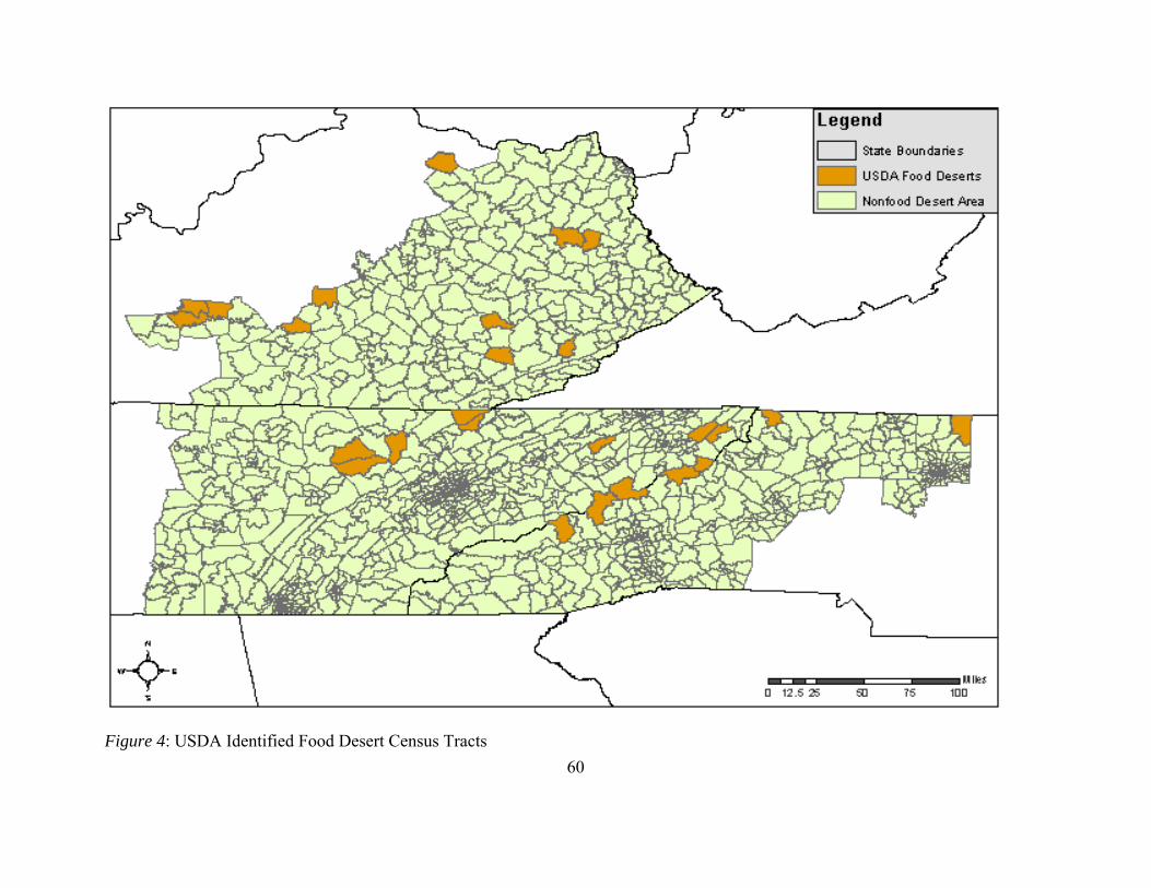
60
Figure 4: USDA Identified Food Desert Census Tracts
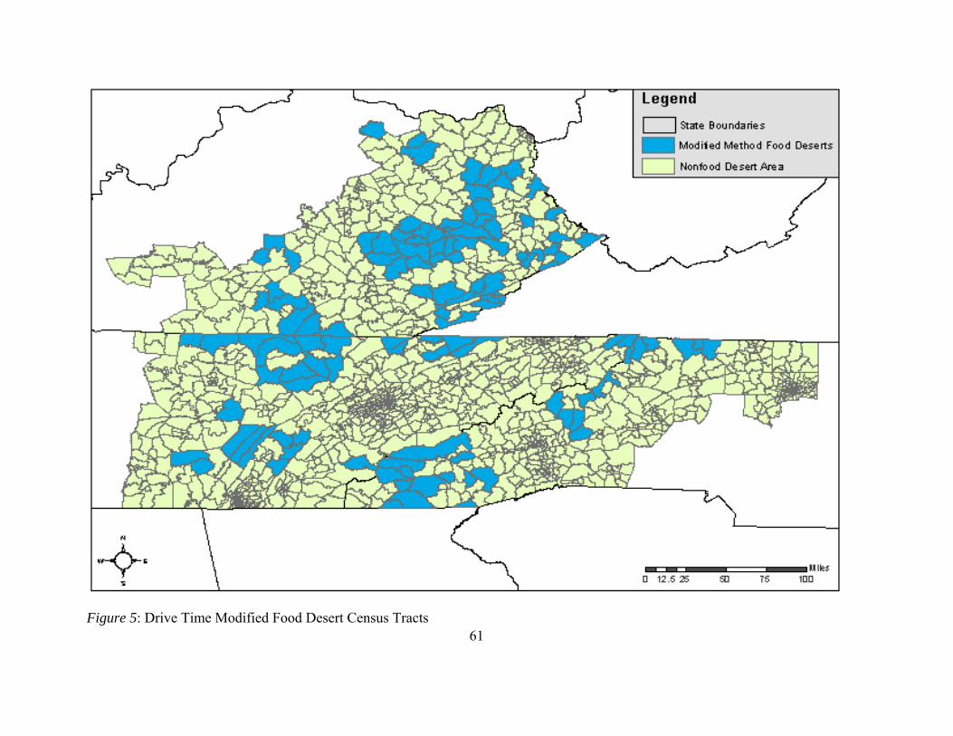
61
Figure 5: Drive Time Modified Food Desert Census Tracts
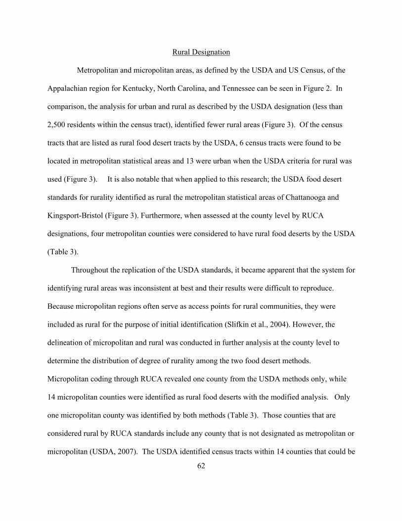
62
Rural Designation
Metropolitan and micropolitan areas, as defined by the USDA and US Census, of the
Appalachian region for Kentucky, North Carolina, and Tennessee can be seen in Figure 2. In
comparison, the analysis for urban and rural as described by the USDA designation (less than
2,500 residents within the census tract), identified fewer rural areas (Figure 3). Of the census
tracts that are listed as rural food desert tracts by the USDA, 6 census tracts were found to be
located in metropolitan statistical areas and 13 were urban when the USDA criteria for rural was
used (Figure 3). It is also notable that when applied to this research; the USDA food desert
standards for rurality identified as rural the metropolitan statistical areas of Chattanooga and
Kingsport-Bristol (Figure 3). Furthermore, when assessed at the county level by RUCA
designations, four metropolitan counties were considered to have rural food deserts by the USDA
(Table 3).
Throughout the replication of the USDA standards, it became apparent that the system for
identifying rural areas was inconsistent at best and their results were difficult to reproduce.
Because micropolitan regions often serve as access points for rural communities, they were
included as rural for the purpose of initial identification (Slifkin et al., 2004). However, the
delineation of micropolitan and rural was conducted in further analysis at the county level to
determine the distribution of degree of rurality among the two food desert methods.
Micropolitan coding through RUCA revealed one county from the USDA methods only, while
14 micropolitan counties were identified as rural food deserts with the modified analysis. Only
one micropolitan county was identified by both methods (Table 3). Those counties that are
considered rural by RUCA standards include any county that is not designated as metropolitan or
micropolitan (USDA, 2007). The USDA identified census tracts within 14 counties that could be
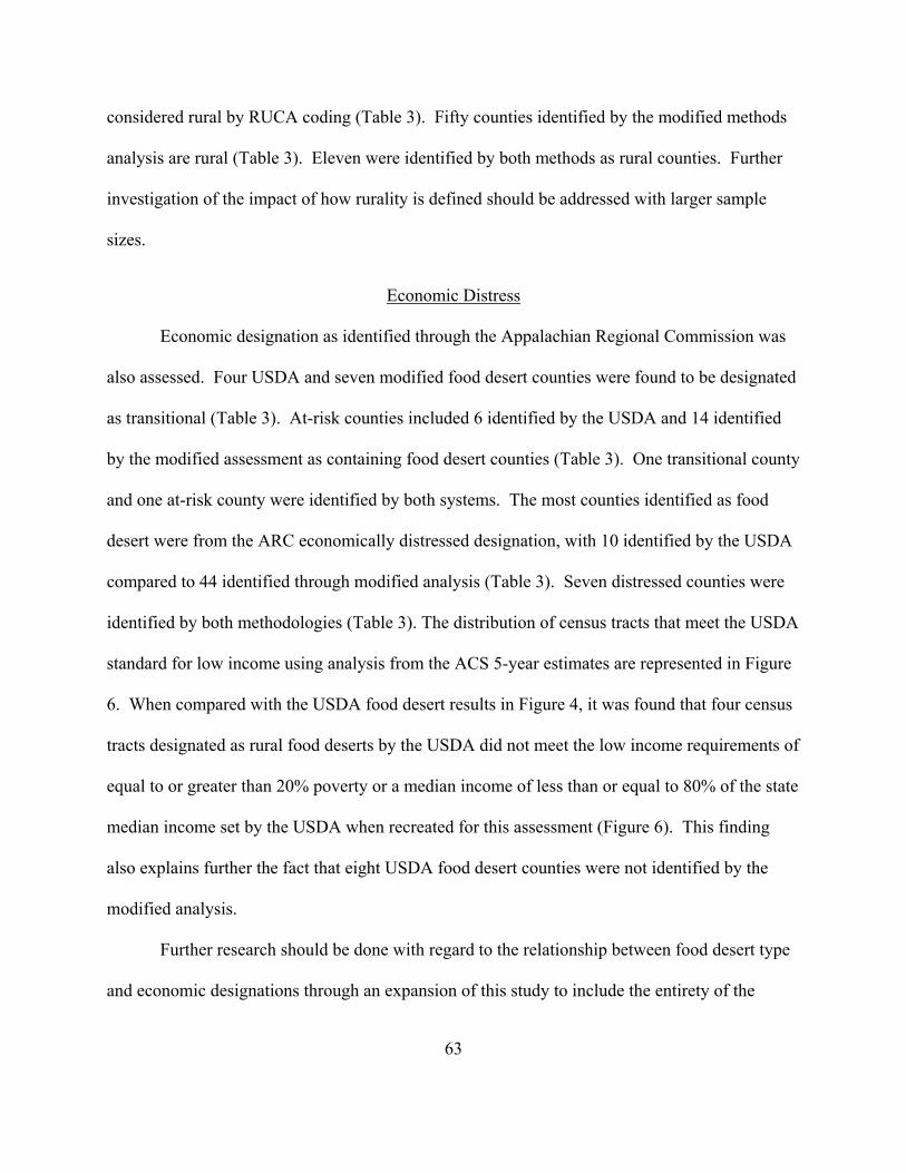
63
considered rural by RUCA coding (Table 3). Fifty counties identified by the modified methods
analysis are rural (Table 3). Eleven were identified by both methods as rural counties. Further
investigation of the impact of how rurality is defined should be addressed with larger sample
sizes.
Economic Distress
Economic designation as identified through the Appalachian Regional Commission was
also assessed. Four USDA and seven modified food desert counties were found to be designated
as transitional (Table 3). At-risk counties included 6 identified by the USDA and 14 identified
by the modified assessment as containing food desert counties (Table 3). One transitional county
and one at-risk county were identified by both systems. The most counties identified as food
desert were from the ARC economically distressed designation, with 10 identified by the USDA
compared to 44 identified through modified analysis (Table 3). Seven distressed counties were
identified by both methodologies (Table 3). The distribution of census tracts that meet the USDA
standard for low income using analysis from the ACS 5-year estimates are represented in Figure
6. When compared with the USDA food desert results in Figure 4, it was found that four census
tracts designated as rural food deserts by the USDA did not meet the low income requirements of
equal to or greater than 20% poverty or a median income of less than or equal to 80% of the state
median income set by the USDA when recreated for this assessment (Figure 6). This finding
also explains further the fact that eight USDA food desert counties were not identified by the
modified analysis.
Further research should be done with regard to the relationship between food desert type
and economic designations through an expansion of this study to include the entirety of the
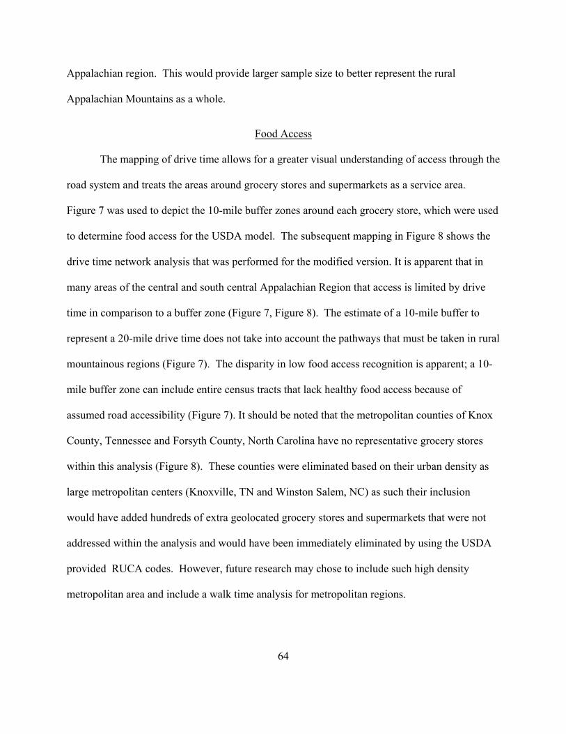
64
Appalachian region. This would provide larger sample size to better represent the rural
Appalachian Mountains as a whole.
Food Access
The mapping of drive time allows for a greater visual understanding of access through the
road system and treats the areas around grocery stores and supermarkets as a service area.
Figure 7 was used to depict the 10-mile buffer zones around each grocery store, which were used
to determine food access for the USDA model. The subsequent mapping in Figure 8 shows the
drive time network analysis that was performed for the modified version. It is apparent that in
many areas of the central and south central Appalachian Region that access is limited by drive
time in comparison to a buffer zone (Figure 7, Figure 8). The estimate of a 10-mile buffer to
represent a 20-mile drive time does not take into account the pathways that must be taken in rural
mountainous regions (Figure 7). The disparity in low food access recognition is apparent; a 10-
mile buffer zone can include entire census tracts that lack healthy food access because of
assumed road accessibility (Figure 7). It should be noted that the metropolitan counties of Knox
County, Tennessee and Forsyth County, North Carolina have no representative grocery stores
within this analysis (Figure 8). These counties were eliminated based on their urban density as
large metropolitan centers (Knoxville, TN and Winston Salem, NC) as such their inclusion
would have added hundreds of extra geolocated grocery stores and supermarkets that were not
addressed within the analysis and would have been immediately eliminated by using the USDA
provided RUCA codes. However, future research may chose to include such high density
metropolitan area and include a walk time analysis for metropolitan regions.
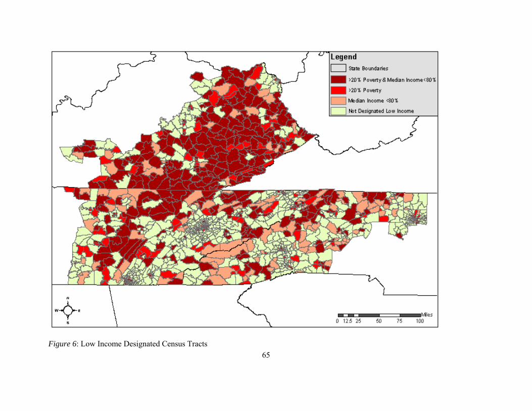
65
Figure 6: Low Income Designated Census Tracts
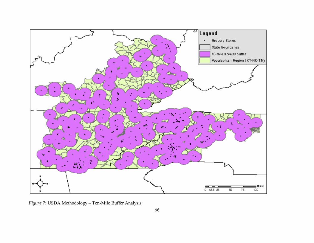
66
Figure 7: USDA Methodology – Ten-Mile Buffer Analysis
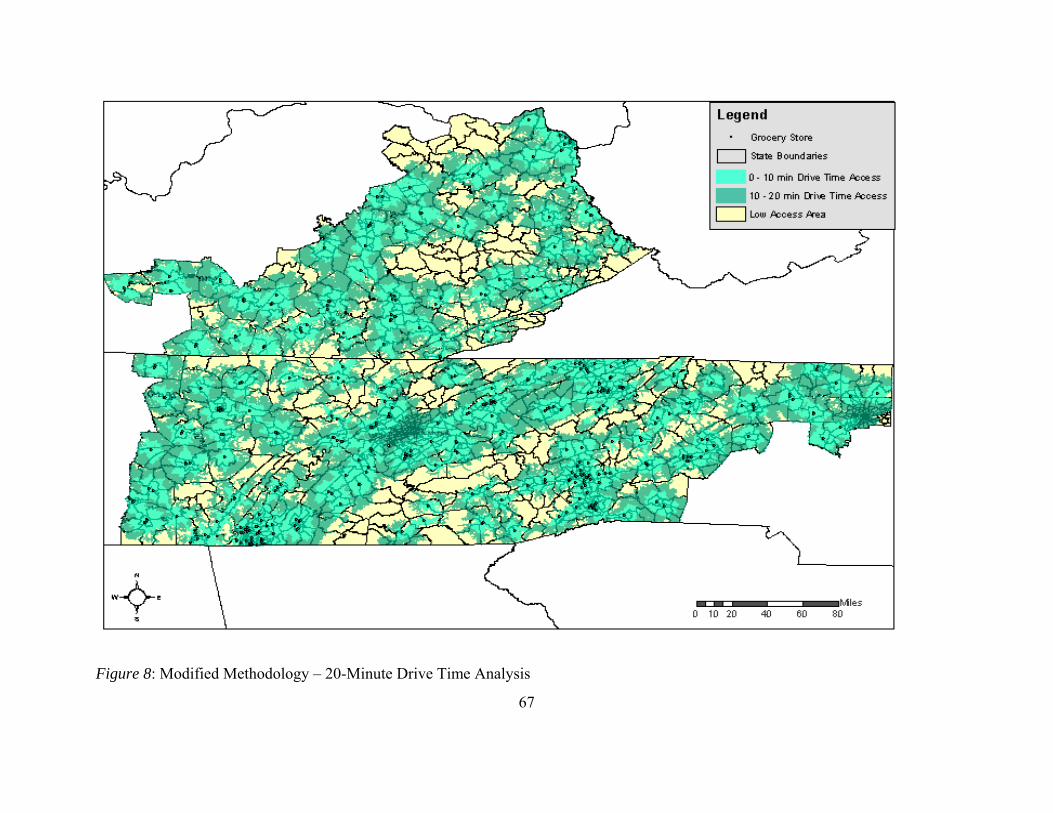
67
Figure 8: Modified Methodology – 20-Minute Drive Time Analysis
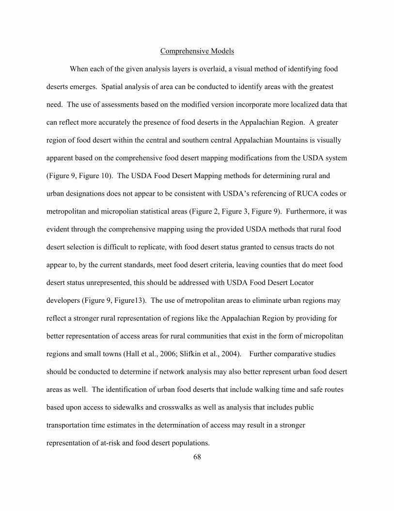
68
Comprehensive Models
When each of the given analysis layers is overlaid, a visual method of identifying food
deserts emerges. Spatial analysis of area can be conducted to identify areas with the greatest
need. The use of assessments based on the modified version incorporate more localized data that
can reflect more accurately the presence of food deserts in the Appalachian Region. A greater
region of food desert within the central and southern central Appalachian Mountains is visually
apparent based on the comprehensive food desert mapping modifications from the USDA system
(Figure 9, Figure 10). The USDA Food Desert Mapping methods for determining rural and
urban designations does not appear to be consistent with USDA’s referencing of RUCA codes or
metropolitan and micropolian statistical areas (Figure 2, Figure 3, Figure 9). Furthermore, it was
evident through the comprehensive mapping using the provided USDA methods that rural food
desert selection is difficult to replicate, with food desert status granted to census tracts do not
appear to, by the current standards, meet food desert criteria, leaving counties that do meet food
desert status unrepresented, this should be addressed with USDA Food Desert Locator
developers (Figure 9, Figure13). The use of metropolitan areas to eliminate urban regions may
reflect a stronger rural representation of regions like the Appalachian Region by providing for
better representation of access areas for rural communities that exist in the form of micropolitan
regions and small towns (Hall et al., 2006; Slifkin et al., 2004). Further comparative studies
should be conducted to determine if network analysis may also better represent urban food desert
areas as well. The identification of urban food deserts that include walking time and safe routes
based upon access to sidewalks and crosswalks as well as analysis that includes public
transportation time estimates in the determination of access may result in a stronger
representation of at-risk and food desert populations.

69
Figure 9: USDA Methodology Model
70
Figure 10: Modified Methodology Model
71
Health Outcomes
Obesity
For county level estimates health outcomes, 70.59% of the counties identified through the
modified method only reported obesity (self-reported BMI of 30 or higher) in equal to or greater
than 29.8% of the county population (Table 4). The USDA method reported county level obesity
estimates equal to or greater than 29.8% of the county population for 75% of its counties (Table
4). Results from both methodologies identified a majority of counties with self-reported obesity
rates within the highest category identified by the National Diabetes Surveillance System
(Centers for Disease Control and Prevention: National Diabetes Surveillance System, 2011). No
counties identified through either method of food desert analysis had obesity rates falling below
22% of the county population (Table 4). It appears that counties within food desert designations,
regardless of the methodology, have a percent obese population within the highest range.
Categorical obesity rates by county were analyzed through both univariate analysis and
multivariate regression analysis. The multivariate analysis controlled for rural severity (RUCA
designation) and economic designation (Table 5). It was hypothesized that because both
methodologies should represent the same populations that their health outcome rates should be
similar. The adjusted odds ratio of obesity rates and food desert methodology type, food desert
methodology does not significantly affect obesity rates (Table 5). Neither micropolitan nor rural
RUCA designations had any significant affect on diabetes diagnosis (Table 5). While these are
not significant, small sample size may have influenced these results and further investigation
with larger sample sizes may shed more light onto any potential influence food desert analysis
72
variations and rurality may have. Crude odds ratios suggested that both at-risk (p <0.05) and
distressed (p <0.01) counties significantly influence obesity (Table 5). However, the adjusted
odds determined that only the distressed economic designation significantly impacts obesity
(Table 5). When compared with transitional food desert counties, distressed counties were
almost 40 times more likely to have higher rates of obesity (44.46; CI = 5.41, 365.45 (Table 5).
This link between economic designation and obesity rates reflects the current literature related to
neighborhood deprivation and BMI, that state that as socioeconomic status and income level
decrease, obesity prevalence rates and the risk of overweight and obesity (Babey et al., 2008;
Hosler, 2009; Macdonald et al., 2011; Powell & Bao, 2009; Powell et al., 2010). However,
because the results are based upon such a small sample size, further investigation should be
conducted to confirm these results because the sample size was not large enough to maintain the
regression.
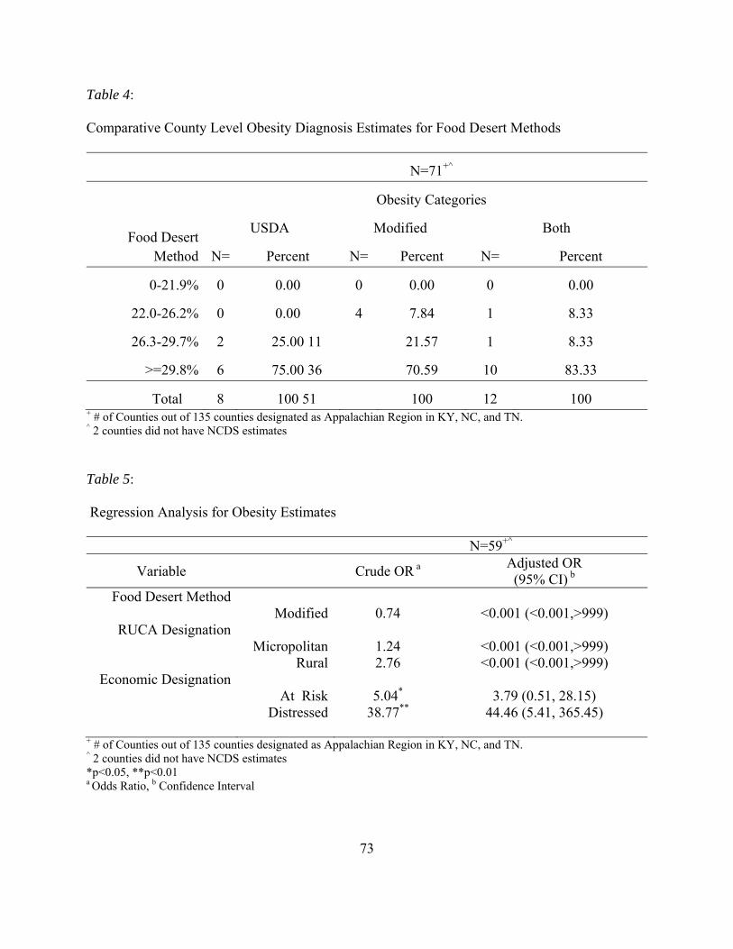
73
Table 4:
Comparative County Level Obesity Diagnosis Estimates for Food Desert Methods
N=71+^
Obesity Categories
Food Desert Method
USDA Modified Both
N= Percent N= Percent N= Percent
0-21.9% 0 0.00 0 0.00 0 0.00
22.0-26.2% 0 0.00 4 7.84 1 8.33
26.3-29.7% 2 25.00 11 21.57 1 8.33
>=29.8% 6 75.00 36 70.59 10 83.33
Total 8 100 51 100 12 100 + # of Counties out of 135 counties designated as Appalachian Region in KY, NC, and TN. ^ 2 counties did not have NCDS estimates
Table 5:
Regression Analysis for Obesity Estimates
N=59+^
Variable Crude OR a Adjusted OR (95% CI) b
Food Desert Method Modified 0.74 <0.001 (<0.001,>999)
RUCA Designation Micropolitan 1.24 <0.001 (<0.001,>999) Rural 2.76 <0.001 (<0.001,>999)
Economic Designation At Risk 5.04* 3.79 (0.51, 28.15) Distressed 38.77** 44.46 (5.41, 365.45)
+ # of Counties out of 135 counties designated as Appalachian Region in KY, NC, and TN. ^ 2 counties did not have NCDS estimates *p<0.05, **p<0.01 a Odds Ratio, b Confidence Interval

74
Diabetes
The percentage of counties with a rate of diabetes diagnosis greater than or equal to
10.6% of the county population was found to be 37.5% for USDA food desert counties and
58.82% for counties identified by the modified analysis (Table 6). No significant relationship
was found between diabetes diagnosis rate estimates by county and food desert method (p =
0.4868). Of those food deserts that had a diabetes rate of 8.9 – 10.5% of county population, the
USDA results were 50%, while the modified method results were 31.37% (Table 6). No food
desert counties by either methodology that met the diabetes diagnosis rate of equal to or less than
6.3% county population (Table 6). Results from both methodologies identified the majority of
counties have at least 8.9% of their population as diagnosed with diabetes.
County level categorical diabetes diagnosis rates were analyzed through both univariate
analysis and multivariate regression analysis. The multivariate analysis controlled for rural
severity (RUCA designation) and economic designation (Table 7). It was hypothesized that
because both methodologies should represent the same populations, their diabetes diagnosis rates
should be similar. The adjusted odds ratio of diabetes diagnosis rates and food desert
methodology type, food desert methodology does not significantly affect diabetes diagnosis rates
(1.39; CI = 0.17, 11.25) (Table 7). Neither micropolitan nor rural RUCA designations had any
significant affect on diabetes diagnosis (Table 7). The adjusted odds ratio determined that only
the distressed economic designation significantly impacts diabetes diagnosis (Table 7). When
compared with transitional food desert counties, distressed counties were over 20 times more
likely to have higher rates of diabetes diagnosis (20.90; CI = 3.16, 138.35) (Table 7). The link
between economic distress and diabetes diagnosis rates may be a crucial element in food desert
populations. In previous studies diabetes rates have been related to an increase in access to fast
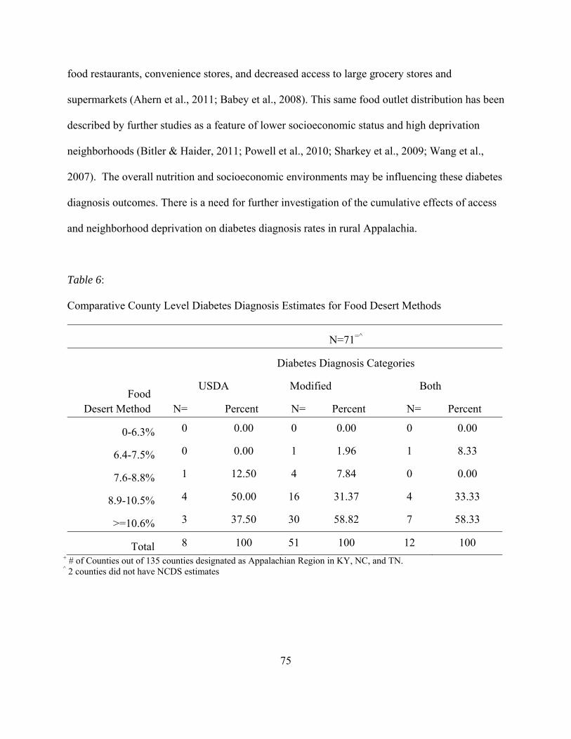
75
food restaurants, convenience stores, and decreased access to large grocery stores and
supermarkets (Ahern et al., 2011; Babey et al., 2008). This same food outlet distribution has been
described by further studies as a feature of lower socioeconomic status and high deprivation
neighborhoods (Bitler & Haider, 2011; Powell et al., 2010; Sharkey et al., 2009; Wang et al.,
2007). The overall nutrition and socioeconomic environments may be influencing these diabetes
diagnosis outcomes. There is a need for further investigation of the cumulative effects of access
and neighborhood deprivation on diabetes diagnosis rates in rural Appalachia.
Table 6:
Comparative County Level Diabetes Diagnosis Estimates for Food Desert Methods
N=71=^
Diabetes Diagnosis Categories
Food Desert Method
USDA Modified Both
N= Percent N= Percent N= Percent
0-6.3% 0 0.00 0 0.00 0 0.00
6.4-7.5% 0 0.00 1 1.96 1 8.33
7.6-8.8% 1 12.50 4 7.84 0 0.00
8.9-10.5% 4 50.00 16 31.37 4 33.33
>=10.6% 3 37.50 30 58.82 7 58.33
Total 8 100 51 100 12 100 + # of Counties out of 135 counties designated as Appalachian Region in KY, NC, and TN. ^ 2 counties did not have NCDS estimates
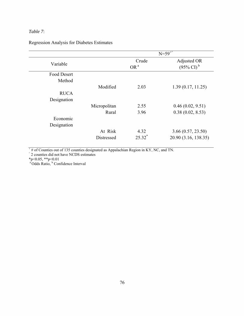
76
Table 7:
Regression Analysis for Diabetes Estimates
N=59+^
Variable Crude
OR a Adjusted OR (95% CI) b
Food Desert Method
Modified 2.03 1.39 (0.17, 11.25) RUCA
Designation Micropolitan 2.55 0.46 (0.02, 9.51) Rural 3.96 0.38 (0.02, 8.53)
Economic Designation
At Risk 4.32 3.66 (0.57, 23.50) Distressed 25.32* 20.90 (3.16, 138.35)
+ # of Counties out of 135 counties designated as Appalachian Region in KY, NC, and TN. ^ 2 counties did not have NCDS estimates *p<0.05, **p<0.01 a Odds Ratio, b Confidence Interval
77
CHAPTER 5
DISCUSSION
Summary
The initial goal of this research was to develop a methodology for using drive time
instead of buffer zones within the USDA’s methodology for designating food deserts in rural
Appalachia. It was determined that drive time can be used as a criteria for food access in the
USDA system for identifying food deserts. While using a network analysis to determine food
access areas is a more complicated procedure than using a buffer zone analysis, it produces
results that are better able to represent actual healthy food access with regard to road type and
topography.
The second specific aim for this research was to determine if the use of drive time
analysis increases the overall area and number of food desert regions identified when compared
to the USDA methods. The modification of drive time does increase the area and number of
food deserts present. This modified food desert system more than tripled the number of counties
identified as containing food deserts when compared to the USDA system. There are concerns
that the USDA model may have further criteria limiting the number of food desert regions with
respect to population distribution and density that involve the designation of rural by the
USDA’s Food Desert Locator.
When comparing health outcome statistics for obesity and diabetes diagnosis between the
two methods of food desert designation, no significant difference was found. This confirmed the
hypothesis that the USDA method and the modified method would represent populations with
78
the same health outcome status and thus there would be no in out come between the two
methods.
Reproducibility
The standards as provided for by the USDA were not as a whole reproducible during the
process of this study. While it is unknown if this is due to a variation in the year of data
procured, with this study using more recent data than the USDA studies, it is clear that other
processes unknown to the outside research were likely used. This study was unable using the
guidelines to fully reproduce the results obtained by the USDA for not only the overall food
desert identification but also in regards to rurality and low income. It is disconcerting that these
measures are not reproducible. To garner a greater level of understanding of the USDA’s
decision-making process with regard to food deserts, it was critical to identify what other factors
were involved in the identification process that were not provided.
Food Access
Food Outlets
During the process of this research, it became evident that not all grocery stores are
created equal. It is imperative when assessing food access based on supermarkets and large
chain grocers that the data all carefully addressed. There are many establishments that maintain
a NAICS code of 445110 that do not meet the requirements set by the USDA and current
literature for supermarket and large chain grocery stores. Through the cleaning process, stores
coded 445110 often were associated with another code and were combination stores instead of
grocery stores. Highlights from these combination stores included; hardware and grocery stores,
liquor and grocery stores, a chain of fireworks warehouses and grocery, an auto repair shop and
79
grocery store, and a used car dealership and grocery store. The current literature suggests that
these combination stores do not provide adequate access to healthy foods (Sharkey et al., 2009).
However, for many rural residents these may be the nearest option for food. This may support
data that show households will often drive beyond the most convenient food outlet option for
better prices, food quality, and variety (Thomas, 2010; Webber & Rojhani, 2010). The rural
practice of ’stockpiling’ food resources is supported by the lack of quality food outlets in these
regions. It is possible that for many households it is worth the investment to drive farther for
better options; however, for those who are of lower economic means this is not always a
practical solution (Thomas, 2010). Vulnerable populations may not be as capable of managing
their food security with the limited options of choosing a more expensive, lower quality food
outlet or drive twice as far less often (Webber & Rojhani, 2010). The second option then
requires access to reliable transportation, and while vehicle access is higher in rural areas, there
is also no public transportation. We must also consider the subset of the rural populations that
regularly go overlooked such as the elderly. Addressing the needs of the most vulnerable
populations in our rural regions is critical when examining food desert designations.
Another way that not all grocery stores are created equal includes chain grocery stores of
variable size. These stores often produce revenues over 2 million dollars a year and were on
WIC lists; however, they are small square footage stores, often less than 4,000 square feet and
often much older building structures. In the course of cleaning data, internet searches to confirm
that food outlets were still in operation, images from googlemaps based searches were available.
Visual inspection of chain grocery stores that meet current access criteria shows a need for a
better system for identifying valid food outlets. An identification system that takes into account
store inventory patterns and age of facility and upgrades to food storage units such as
80
refrigerated produce units would be more comprehensive. Investigation into perceptions of store
quality, safety, and inventory may also be needed to determine whether food outlets meet access
and availability standards.
Assessment of quality of grocery stores is a time consuming and continual process. The
current systems for obtaining food retailer data are not detailed enough to necessarily accurately
represent what exists with regards to supermarkets and large chain grocery stores. At some point
there may be a need for a standardized reporting system for food outlets that maintain coding as
grocery stores. This may, however, be the most difficult from a policy standpoint and would
involve the coordination of multiple commercial markets. However, the collaboration between
food outlet businesses and communities at the local and regional level may lead to positive
change. One key element in developing partnerships between communities and food outlets may
be the creation of incentive based participatory intervention strategies. By incentivizing
improved access to healthy foods in smaller local markets, thorough small grants or subsidies for
food outlets and coupon or other discounts for shoppers, there is the potential improve the
consumer nutrition environment and improve healthy food access while potentially improving
revenue for these food outlets.
Drive Time
Using a 20-minute access range for the network analysis of drive times allowed for a
better visual understanding of access in varying regions. There are many areas within this region
of Appalachia that while they have road access, they are too remote to have grocery store access.
There are many areas where a mail road brings 20-minute access through a portion of a census
tract, likely by way of highways, but beyond the main thoroughfare, there is no food access.
81
These are regions regardless of economic status that could benefit from increased access to
healthy foods. While the greatest risk will always be associated with those regions with both low
access and low income, all individuals with low access are at-risk.
Currently the system for designating food deserts is an all or nothing evaluation. It would
seem to be more effective to have levels of food desert status based upon degrees of access and
income. This would more closely resemble the system set forward by the Appalachian Regional
Commission is their economic status designations (Appalachian Regional Commission, 2012).
Developing an index to assess food desert severity could eliminate the underrepresentation of at-
risk populations, particularly from a rural focus. An index of this nature could take into account
that households residing in rural areas on the 20-minute border of food outlet access that are also
low income are not underrepresented. Committing to 40 minutes in a day to access healthier
food options has its costs. Between the cost of gas, time, and the quantity of food that must be
bought, a low income household at the 20-minute boundary could be an underrepresented
population. This would also be the case for those households with limited transportation access,
in that there is a greater commitment to travel and little or no access to public transportation
means. A tiered system for evaluating food desert and related at-risk populations could be
organized as:
Food Desert: those residents meeting the strictest criteria of outside 20-minute drive
time, designated low income and rural.
At-risk: border region residents (food outlet access between a 15- to 20-minute drive
time), designated low income and not metropolitan.
Low Access: residents of regions that meet the greater than 20-minute drive time;
however, they do not meet the low income requirements.
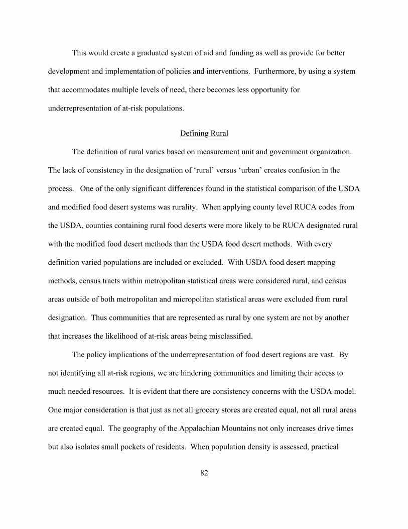
82
This would create a graduated system of aid and funding as well as provide for better
development and implementation of policies and interventions. Furthermore, by using a system
that accommodates multiple levels of need, there becomes less opportunity for
underrepresentation of at-risk populations.
Defining Rural
The definition of rural varies based on measurement unit and government organization.
The lack of consistency in the designation of ‘rural’ versus ‘urban’ creates confusion in the
process. One of the only significant differences found in the statistical comparison of the USDA
and modified food desert systems was rurality. When applying county level RUCA codes from
the USDA, counties containing rural food deserts were more likely to be RUCA designated rural
with the modified food desert methods than the USDA food desert methods. With every
definition varied populations are included or excluded. With USDA food desert mapping
methods, census tracts within metropolitan statistical areas were considered rural, and census
areas outside of both metropolitan and micropolitan statistical areas were excluded from rural
designation. Thus communities that are represented as rural by one system are not by another
that increases the likelihood of at-risk areas being misclassified.
The policy implications of the underrepresentation of food desert regions are vast. By
not identifying all at-risk regions, we are hindering communities and limiting their access to
much needed resources. It is evident that there are consistency concerns with the USDA model.
One major consideration is that just as not all grocery stores are created equal, not all rural areas
are created equal. The geography of the Appalachian Mountains not only increases drive times
but also isolates small pockets of residents. When population density is assessed, practical
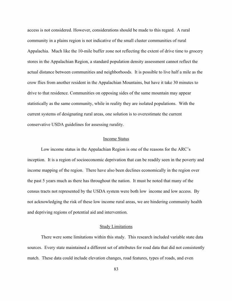
83
access is not considered. However, considerations should be made to this regard. A rural
community in a plains region is not indicative of the small cluster communities of rural
Appalachia. Much like the 10-mile buffer zone not reflecting the extent of drive time to grocery
stores in the Appalachian Region, a standard population density assessment cannot reflect the
actual distance between communities and neighborhoods. It is possible to live half a mile as the
crow flies from another resident in the Appalachian Mountains, but have it take 30 minutes to
drive to that residence. Communities on opposing sides of the same mountain may appear
statistically as the same community, while in reality they are isolated populations. With the
current systems of designating rural areas, one solution is to overestimate the current
conservative USDA guidelines for assessing rurality.
Income Status
Low income status in the Appalachian Region is one of the reasons for the ARC’s
inception. It is a region of socioeconomic deprivation that can be readily seen in the poverty and
income mapping of the region. There have also been declines economically in the region over
the past 5 years much as there has throughout the nation. It must be noted that many of the
census tracts not represented by the USDA system were both low income and low access. By
not acknowledging the risk of these low income rural areas, we are hindering community health
and depriving regions of potential aid and intervention.
Study Limitations
There were some limitations within this study. This research included variable state data
sources. Every state maintained a different set of attributes for road data that did not consistently
match. These data could include elevation changes, road features, types of roads, and even
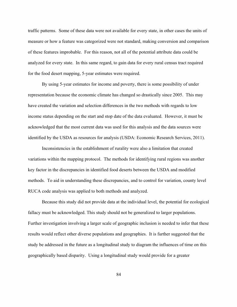
84
traffic patterns. Some of these data were not available for every state, in other cases the units of
measure or how a feature was categorized were not standard, making conversion and comparison
of these features improbable. For this reason, not all of the potential attribute data could be
analyzed for every state. In this same regard, to gain data for every rural census tract required
for the food desert mapping, 5-year estimates were required.
By using 5-year estimates for income and poverty, there is some possibility of under
representation because the economic climate has changed so drastically since 2005. This may
have created the variation and selection differences in the two methods with regards to low
income status depending on the start and stop date of the data evaluated. However, it must be
acknowledged that the most current data was used for this analysis and the data sources were
identified by the USDA as resources for analysis (USDA: Economic Research Services, 2011).
Inconsistencies in the establishment of rurality were also a limitation that created
variations within the mapping protocol. The methods for identifying rural regions was another
key factor in the discrepancies in identified food deserts between the USDA and modified
methods. To aid in understanding these discrepancies, and to control for variation, county level
RUCA code analysis was applied to both methods and analyzed.
Because this study did not provide data at the individual level, the potential for ecological
fallacy must be acknowledged. This study should not be generalized to larger populations.
Further investigation involving a larger scale of geographic inclusion is needed to infer that these
results would reflect other diverse populations and geographies. It is further suggested that the
study be addressed in the future as a longitudinal study to diagram the influences of time on this
geographically based disparity. Using a longitudinal study would provide for a greater
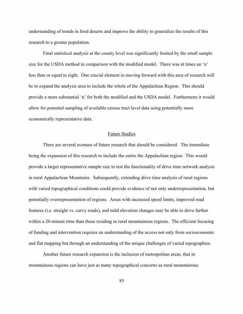
85
understanding of trends in food deserts and improve the ability to generalize the results of this
research to a greater population.
Final statistical analysis at the county level was significantly limited by the small sample
size for the USDA method in comparison with the modified model. There was at times an ‘n’
less than or equal to eight. One crucial element in moving forward with this area of research will
be to expand the analysis area to include the whole of the Appalachian Region. This should
provide a more substantial ‘n’ for both the modified and the USDA model. Furthermore it would
allow for potential sampling of available census tract level data using potentially more
economically representative data.
Future Studies
There are several avenues of future research that should be considered. The immediate
being the expansion of this research to include the entire the Appalachian region. This would
provide a larger representative sample size to test the functionality of drive time network analysis
in rural Appalachian Mountains. Subsequently, extending drive time analysis of rural regions
with varied topographical conditions could provide evidence of not only underrepresentation, but
potentially overrepresentation of regions. Areas with increased speed limits, improved road
features (i.e. straight vs. curvy roads), and mild elevation changes may be able to drive farther
within a 20-minute time than those residing in rural mountainous regions. The efficient focusing
of funding and intervention requires an understanding of the access not only from socioeconomic
and flat mapping but through an understanding of the unique challenges of varied topographies.
Another future research expansion is the inclusion of metropolitan areas, that in
mountainous regions can have just as many topographical concerns as rural mountainous
86
regions. Also, the use of walking time analysis with sidewalk and crosswalk features could
provide better insight in to access in urban communities. It is rare in an urban setting that you
can take a straight line path without going through a building or climbing a fence, and often the
least direct path must be taken. Other aspect that could be included in urban access is public
transportation routes and times. There are many blended options within urban communities and
increased pedestrian concerns including traffic safety and crime rates to be considered when
access to food outlets is concerned.
Contribution to Public Health
This research was based on identifying underrepresented populations within rural
Appalachia. It is crucial to identify all at-risk populations when assessing health environment
concerns. It is clear from the research that the USDA model for assessing food deserts does not
take into account topography. No two regions of the United States are exactly the same
geographically. To apply the same criteria to the Appalachian Region, the Gulf Coast, or the
Rocky Mountains without addressing the unique geography that allows for small rural
communities residing in mountains, entire communities lose their voice. To lose representation
with regards to the health of the community is a concern. Underrepresented areas are not only
unacknowledged as having need, but they cannot contribute to solutions or gain the needed
support through policy and interventions. Without acknowledgment of their food access issues,
this lack of access perpetuates and could become worse. This research contributes a model that
represents other unacknowledged food deserts in a geographically unique region. This research
and its methodology need to be expanded to evaluate other unique geographic regions that could
contain food deserts hidden by the current evaluation system.
87
REFERENCES
Ahern, M., Brown, C., & Dukas, S. (2011). A national study of the association between food
environments and county-level health outcomes. The Journal of Rural Health, 27, 367-
379. doi:10.1111/j.1748-0361.2011.00378.x
Amberg, R., & Hill, I. T. (Ed.). (2002). Sodom Laurel album. Chapel Hill: The University of
North Carolina Press.
Appalachian Regional Commission. (2012). Research, maps, and data. Retrieved February 9,
2012, from Appalachian Regional Commission:
http://www.arc.gov/research/RegionalDataandResearch.asp
Appalachian Regional Commission A. (2011a). Distressed areas in Appalachian Kentucky,
fiscal year 2012. Retrieved February 21, 2012, from
http://www.arc.gov/images/appregion/economic_statusFY2012/CountyEconomicStatusa
ndDistressAreasFY2012Kentucky.pdf
Appalachian Regional Commission B. (2011b, April). County economic status and number of
distressed areas in Appalachian North Carolina, fiscal year 2012. Retrieved February 21,
2012, from
http://www.arc.gov/images/appregion/economic_statusFY2012/CountyEconomicStatusa
ndDistressAreasFY2012NorthCarolina.pdf
Appalachian Regional Commission C. (2011c, April). County economic status and number of
distressed areas in Appalachian Tennessee, fiscal year 2012. Retrieved February 21,
2012, from
http://www.arc.gov/images/appregion/economic_statusFY2012/CountyEconomicStatusa
ndDistressAreasFY2012Tennessee.pdf
88
Babey, S., Diamant, A., Hasert, T., & Harvey, S. (2008, April 1). Designed for disease: The line
between local food environments and obesity and diabetes. UCLA Center for Health
Policy Research.
Beaulac, J., Kristjansson, E., & Cummins, S. (2009, July). A systematic review of food deserts,
1966-2007. Preventing Chronic Disease, 6, A105. Retrieved from
www.cdc.gov/pcd/issues/2009/jul/08_0163.htm
Bitler, M., & Haider, S. J. (2011). An economic view of food deserts in the United States.
Journal of Policy Analysis and Management, 30, 153-176. doi:10.1002/pam.20550
Black, J. L., & Macinko, J. (2008). Neighborhoods and obesity. Nutrition Reviews, 66, 2-20.
doi:10.1111/j.1753-4887.2007.00001.x
Blanchard, T., & Lyson, T. (2002). Access to low cost groceries in nonmetropolitan counties:
Large retailers and the creation of food deserts. Measuring Rural Diversity, (pp. 1-24).
Washington DC.
Centers for Disease Control and Prevention: National Diabetes Surveillance System. (2011,
December). Diabetes data & trends. Retrieved February 25, 2012, from Centers for
Disease Control and Prevention: http://apps.nccd.cdc.gov/DDTSTRS/default.aspx.
Chang, K.-t. (2010). Introduction to geographic information systems (5th ed.). New York, NY:
McGraw Hill Higher Education.
Chen, S., Florax, R. J., Snyder, S., & Miller, C. C. (2010). Obesity and access to chain grocers.
Economic Geography, 86, 431-452.
Cummins, S., & Macintyre, S. (2006). Food environments and obesity - Neighbourhood or
nation? International Journal of Epidemiology, 35, 100-104. doi:10.1093/ije/dyi276
89
Cummins, S., Smith, D., Taylor, M., Dawson, J., Marshall, D., Sparks, L., & Anderson, A.
(2009). Variations in fresh fruit and vegetable quality by store type, urban-rural setting
and neighbourhood deprivation in Scotland. Public Health Nutrition, 12, 2044-2050.
doi:doi:10.1017/S1368980009004984
Day, P. L., & Pearce, J. (2011). Obesity-promoting food environments and the spatial clustering
of food outlets around schools. American Journal of Preventative Medicine, 40, 113-121.
doi:10.1016/j.amepre.2010.10.018
Dean, W. R., & Sharkey, J. R. (2011). Rural and urban differences in the associations between
characteristics of the community food environment and fruit and vegetable intake.
Journal of Nutrition Education and Behavior, 1-8. doi:10.1016/j.jneb.2010.07.001
Environmental Systems Research Institute, Inc. (Esri). (2012). What is GIS? Retrieved March 9,
2012, from ESRI Home Page: http://www.esri.com/what-is-
gis/overview.html#overview_panel
Ford, P., & Dzewaltowski, D. A. (2011). Neighborhood deprivation, supermarket availability
and BMI in low-income women: A multilevel analysis. Journal of Community Health,
36, 785-796. doi:10.1007/s10900-011-9377-3
Forsyth, A., Lytle, L., & Van Riper, D. (2010, April 1). Finding food: Issues and challenges in
using geographic information systems to measure food access. Journal of Transportation
Land Use, 3, 43-65. doi:10.5198/jtlu.v3i105
Furey, S., Farley, H., & Strugnell, C. (2002). An investigation into the availability and economic
accessibility of food items in rural and urban areas of Northern Ireland. International
Journal of Consumer Studies, 26, 313-321.
90
Glanz, K., Sallis, J. F., Saelens, B. E., & Frank, L. D. (2005, May/June). Healthy nutrition
environments: Concepts and measures. American Journal of Health Promotion, 19, 330-
333.
Hall, S. A., Kaufman, J. S., & Ricketts, T. C. (2006). Defining urban and rural areas in U.S.
epidemiologic studies. Journal of Urban Health, 83, 162-175. doi:0.1007/s11524-005-
9016-3
Hallett, L. F., & McDermott, D. (2010). Quantifying the extent and cost of food deserts in
Lawrence, Kansas, USA. Applied Geography, 1-6. doi:10.1016/j.apgeog.2010.09.006
Hamelin, A.-M., & Beaudry, M. H.-P. (2002, January). Characterization of household food
insecurity in Quebec: Food and feelings. Social Science and Medicine, 54, 119-132.
doi:10.1016/S0277-9536(01)00013-2
Hill, J. O., & Peters, J. C. (1998, May 28). Environmental contributions to the obesity epidemic.
Science, 280, 1371-1374.
Hoover's. (2012). Hoover's lead builder purchases and saved searches. (Hoover's) Retrieved
February 13, 2012, from Hoover's A D & B Company:
http://subscriber.hoovers.com/H/myHoovers/savedSearches.html
Hosler, A. S. (2009). Retail food availability, obesity, and cigarette smoking in rural
communities. The Journal of Rural Health, 25, 203-210.
Jennings, A., Welch, A., Jones, A. P., Harrison, F., Bentham, G., van Sluijs, E. M., Cassidy, A.
(2011). Local food outlets, weight status, and dietary intake: Associations in children
aged 9-10 years. American Journal of Preventative Medicine, 40, 405-410.
91
Jilcott, S. B., Liu, H., Moore, J. B., Bethel, J. W., Wilson, J., & Ammerman, A. S. (2010).
Commute times, food retail gaps, and body mass index in North Carolina counties.
Preventing Chronic Dease, 7, 1-10. Retrieved January 2012, from
http://www.cdc.gov/pcd/issues/2010/sep/09_0208.htm
Kentucky State Legislature. (2007, June 26). Kentucky Code 180.390: Speed. Retrieved February
8, 2012, from Kentucky Legislature: Kentucky Revised Statutes:
http://www.lrc.ky.gov/KRS/189-00/390.PDF
Larson, N. I., Story, M. T., & Nelson, M. C. (2009). Neighborhood environments: Disparities in
access to healthy foods in the U.S. American Journal of Preventative Medicine, 36, 74-
81. doi:10.1016/j.amepre.2008.09.025
Lebel, A., Pampalon, R., Hamel, D., & Theriault, M. (2009). The geography of overweight in
Quebec: A multilevel perspective. Canadian Journal of Public Health, 100, 18-23.
Liese, A. D., Weis, K. E., Delores, P., Smith, E., & Lawson, A. (2007). Foos store types,
availability, and cost of foods in a rural environment. Journal of the American Dietetic
Association, 107, 1916-1923. doi:10.1016/j.jada.2007.08.012
Liu, G., Wilson, J., Qi, R., & Ying, J. (2007, March/April). Green neighborhoods, food retail and
childhood overweight: Differences by population density. American Journal of Health
Promotion, 21, 317-325.
Macdonald, L., Ellaway, A., Ball, K., & Macintyre, S. (2011). Is proximity to a food retail store
associated with diet and BMI in Glasgow, Scotland? BMC Public Health, 11, 464-473.
doi:http://www.biomedcentral.com/1471-2458/11/464
92
McEntee, J., & Agyeman, J. (2009). Towards the development of a GIS method for identifying
rural food deserts: Geographic access in Vermont, USA. Applied Geography, 1-12.
doi:10.1016/j.apgeog.2009.05.004
McKinnon, R., Reedy, J., Handy, S., & Rodgers, A. (2009, April). Measuring the food and
physical activity environments: Shaping the research agenda. American Journal of
Preventative Medicine, 36, S81-S85. doi:doi:10.1016/j.amepre.2009.01.003
McLafferty, S. L. (2003). GIS and health care. Annual Review of Public Health, 24, 25-42.
doi:10.1146/annurev.publhealth.24.012902.141012
Michimi, A., & Wimberly, M. C. (2010). Associations of supermarket accessibility with obesity
and fruit and vegetable consumption in the conterminous United States. International
Journal of Health Geographics, 9, 1-14. Retrieved from http://www.ij-
healthgeographics.com/content/9/1/49
Morland, K. B., & Evenson, K. R. (2009). Obesity prevalence and the local food environment.
Health and Place, 15, 491-495. doi:10.1016/j.healthplace.2008.09.004
NCDOT: GIS Unit. (2012, February 13). NCDOT GIS data layers. Retrieved February 14, 2012,
from North Carolina Department of Transportation:
http://www.ncdot.gov/it/gis/DataDistribution/DOTData/default.html
Papas, M. A., Alberg, A. J., Ewing, R., Helzlsouer, K. J., Gary, T. L., & Klassen, A. C. (2007).
The built environment and obesity. Epidemiologic Reviews, 29, 129-143.
doi:10.1093/epirev/mxm009
Pearce, J., Witten, K., & Bartie, P. (2006). Neighbourhoods and health: a GIS approach to
measuring community resource accessibility. Journal of Epidemiology and Community
Health, 60, 389-395. doi:10.1136/jech.2005.043281
93
Pearson, T., Russell, J., Michael, C., & Barker, M. (2005). Do ‘food deserts’ influence fruit and
vegetable consumption?—a cross-sectional study. Appetite, 45, 195-197.
doi:10.1016/j.appet.2005.04.003
Powell, L. M., & Bao, Y. (2009). Food prices, access to food outlets and child weight.
Economics and Human Biology, 7, 64-72. doi:10.1016/j.ehb.2009.01.004
Powell, L., Han, E., & Chaloupka, F. (2010). Economic contextual factors, food consumption,
and obesity among US adolescents. The Journal of Nutrition, 140, 1175-1180.
doi:10.3945/jn.109.111526
Sallis, J., Brian, S., Frank, L., Conway, T., Slymen, D., Cain, K., & Kerr, J. (2009).
Neighborhood built environment and income: Examining multiple health outcomes.
Social Science & Medicine, 68, 1285-1293. doi:10.1016/j.socscimed.2009.01.017
Schafft, K. A., Jensen, E. B., & Hinrichs, C. C. (2009). Food deserts and overweight school
children: Evidence from Pennsyvania. Rural Sociology, 74, 153-177.
Sharkey, J. R., Horel, S., & Dean, W. R. (2010). Neighborhood deprivation, vehicle ownership,
and potential spatial access to a variety of fruits and vegetables in a large rural area in
Texas. International Journal of Health Geographics, 9, 1-27. Retrieved from
http://www.ij-healthgeographics.com/content/9/1/26
Sharkey, J., Horel, S., Han, D., & Huber, J. (2009). Associations between neighborhood need
and spatial access to food stores and fast food restaurants of Colonais. International
Journal of Health Geographics, 8. doi:doi:10.1186/1476-072X-8-9
94
Sharkey, J., Johnson, C., Dean, W., & Horel, S. (2011). Focusing on fast food restaurants alone
underestimates the relationship between neighborhood deprivation and exposure to fast
food in a large rural area. Nutrition Journal, 10. Retrieved from
ttp://www.nutritionj.com/content/10/1/10
Slifkin, R. T., Randolph, R., & Ricketts, T. C. (2004). The changing metropolitan designation
process and rural America. The Journal of Rural Health, 20, 1-6.
Smith, D. M., Cummins, S., Taylor, M., Dawson, J., Marshall, D., Sparks, L., & Anderson, A. S.
(2010). Neighbourhood food environment and area deprivation: spatial accessibility to
grocery stores selling fresh fruit and vegetables in urban and rural settings. International
Journal of Epidemiology, 39, 277-284. doi:10.1093/ije/dyp221
Stokols, D. (1996). Translating social ecological theory into guidelines for community health
promotion. American Journal of Health Promotion, 10, 282-298.
Story, M., Kaphingst, K. M., Robinson-O'Brien, R., & Glanz, K. (2008). Creating healthy food
and eating environments: Policy and environmental approaches. Annual Review of Public
Health, 29, 253-272. doi:10.1146/annurev.publhealth.29.020907.090926
Tennessee State Legislature. (2012). Tenn. Code Ann. § 55-8-101. Retrieved February 15, 2012,
from Lexis Nexis: http://www.lexisnexis.com/hottopics/tncode/
Thomas, B. (2010). Food deserts and the sociology of space: Distance to food retailers and food
insecurity in an urban American neighborhood. Engineering and Technology, 67, 19-28.
US Census Burearu, Geography Division. (2011, December 19). TIGER Products: Topologically
Integrated Geographic Encoding and Referencing system. Retrieved February 6, 2012,
from United States Census Bureau: http://www.census.gov/geo/www/tiger/index.html
95
US Census Bureau. (2012, January 11). North Amercian Classification System. Retrieved March
27, 2012, from United States Census Bureau: http://www.census.gov/eos/www/naics/
US Census Bureau: American FactFinder. (2012). US Census Buearu. Retrieved February 5,
2012, from American FactFinder:
http://factfinder2.census.gov/faces/nav/jsf/pages/index.xhtml
USDA. (2004, 4 28). Measuring rurality: Rural-urban continuum codes. Retrieved 2 15, 2012,
from USDA ERS: Briefing Rooms:
http://www.ers.usda.gov/Briefing/Rurality/RuralUrbCon/
USDA. (2007, March 22). Measuring rurality: What is rural. Retrieved 3 12, 2010, from USDA
Economic Research Service: Briefing Rooms:
http://www.ers.usda.gov/Briefing/Rurality/WhatisRural/
USDA. (2011, May 2). USDA introduces online tool for locating 'food deserts'. Retrieved March
10, 2012, from United States Department of Agriculture: News Releases:
http://www.usda.gov/wps/portal/usda/usdahome?contentid=2011/05/0191.xml
USDA: Economic Research Services. (2011, April 15). Food desert locator. Retrieved from ERS
Mapping and Spatial Data Center:
http://www.ers.usda.gov/Data/FoodDesert/foodfesert.html
USDA: Economic Research Services. (n.d.). Food Desert Locator. Retrieved from Food Desert
Locator: Documentation: http://www.ers.usda.gov/Data/FoodDesert/documentation.html
Wang, M. C., Kim, S., Gonzalez, A. A., MacLeod, K. E., & Winkleby, M. A. (2007).
Socioeconomic and food-related physical characteristics of the neighbourhood
environment are associated with body mass index. Journal of Epidemiology and
Community Health, 61, 491-498. doi:10.1136/jech.2006.051680
96
Webber, C., & Rojhani, A. (2010). Food or fuel: Rising gasoline prices and food access among
WIC famililies in non-metropolitan southwest Michigan. Journal of Hunger and
Environmental Nutrition, 5, 484-497. doi:10.1080/19320248.2010.527279
Wendel-Vos, W., Droomers, M., Kremers, S., Brug, J., & van Lenthe, F. (2007). Potential
environmental determinants of physical activity in adults: a systematic review. Obesity
Reviews, 8, 425-440. doi:10.1111/j.1467-789X.2007.00370.x
White, M. (2007). Food access and obesity. Obesity Reviews, 8(Suppl. 1), 99-107.
Wrigley, N., Warm, D., & Margetts, B. (2003). Deprivation, diet, and food-retail access:
Findings from the Leeds `food deserts' study. Environment and Planning, 35, 151-188.
doi:DOI:10.1068/a35150
Yousefian, A., Leighton, A., Fox, K., & Hartley, D. (2011). Understanding the rural food
environment perspectives of low-income parents. Rural and Remote Health, 11, 1631.
Zenk, S., Schult, A., Israel, B., James, S., Bao, S., & Wilson, M. (2005, April). Neighborhood
racial composition, neighborhood poverty and the spacial accessibility of supermarkets in
metropolitan Detroit. American Journal of Public Health, 95, 660-667.
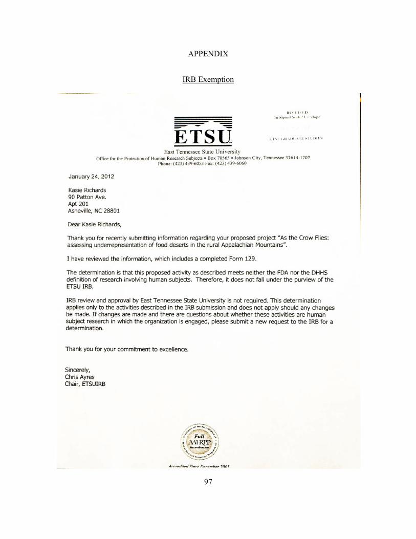
97
APPENDIX
IRB Exemption
98
VITA
KASIE A. RICHARDS
Personal Data: Date of Birth: September 17, 1978 Place of Birth: Birmingham, Alabama Marital Status: Married
Education: DrPH Community and Behavioral Health, East Tennessee State
University, Johnson City, Tennessee, 2012 M.S. Exercise Sports Science (Exercise Physiology), Appalachian
State University, Boone, North Carolina 2003 B.A. Exercise Sports Science (Athletic Training), University of
North Carolina, Chapel Hill, North Carolina 2000 Public Schools, Wilmington, North Carolina
Professional Experience: Research Assistant, Team Up for Healthy Living Project, East
Tennessee State University, Department of Community and Behavioral Health, 2011 – present
Researcher, NOAA tsunami social science project, East Tennessee State University, Department of Geosciences, 2011 – present
Teaching Assistant, East Tennessee State University, Department of Community and Behavioral Health, 2011
Researcher, Tsunami Evacuation Survey, East Tennessee State University, Department of Geosciences, American Samoa, summer 2011
Research Assistant, TN Coordinated School Health Evaluation Grant, East Tennessee State University, Department of Community and Behavioral Health, 2009 – 2010
Clinical Education Coordinator / Assistant Athletic Trainer, Mars Hill College, Mars Hill, North Carolina, 2007 –2008
Faculty Instructor, Biology and Athletic Training Departments, Mars Hill College 2005 – 2008
Recruitment and Retention Coordinator/ Assistant Athletic Trainer Mars Hill College, Mars Hill, North Carolina, 2005 –2007
Adjunct Faculty, Biology and Physical Education Departments, Ashville Buncombe Technical Community College, Asheville, North Carolina 2004 –2005
Honors and Awards: Outstanding DrPH Student 2012, Department of Community and
Behavioral Health, East Tennessee State University Golden Key International Honors Society 2010 - present
Recommended