CE 472 Water Resources Engineering Lab II
(Lab Manual)
Department of Civil Engineering Ahsanullah University of Science and Technology
November, 2017
Preface
Water Resources Engineering is an important field of Civil Engineering. Water is the most
precious natural resource but it can cause severe problems if it is not properly used. So
proper utilization and management of water is necessary especially in the field of irrigation.
Knowledge about Soil properties in an irrigation field, Irrigation Scheduling, Design of
Canal and Analysis of Hydrological data are significant both in Agricultural and Civil
Engineering Field. To meet this purpose, Water Resources Engineering Sessional-II was
introduced. This Lab manual mainly deals with soil properties influencing irrigation such
as- bulk density, soil suction, intake characteristics, coefficient of permeability; canal
seepage loss; abstraction from a single well; irrigation scheduling; design of a branch canal;
frequency analysis of hydrologic data and hydrograph analysis.
This Lab manual was prepared with the help of ‘Irrigation Engineering and Hydraulic
Structures’ by S. K. Garg, and the lab manual ‘Irrigation and Drainage Sessional’ of
Bangladesh University of Engineering and Technology (BUET). The authors highly
indebted to Dr. M. Mirjahan Miah, Professor, Department of Civil Engineering, Ahsanullah
University of Science and Technology for reviewing this manual and giving valuable
comments to improve this manual.
Md. Munirul Islam
Md. Ajwad Anwar
Department of Civil Engineering
Ahsanullah University of Science and Technology
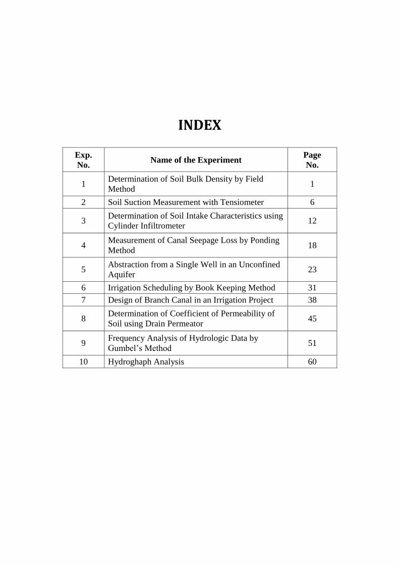
INDEX
Exp.
No. Name of the Experiment
Page
No.
1 Determination of Soil Bulk Density by Field
Method 1
2 Soil Suction Measurement with Tensiometer 6
3 Determination of Soil Intake Characteristics using
Cylinder Infiltrometer 12
4 Measurement of Canal Seepage Loss by Ponding
Method 18
5 Abstraction from a Single Well in an Unconfined
Aquifer 23
6 Irrigation Scheduling by Book Keeping Method 31
7 Design of Branch Canal in an Irrigation Project 38
8 Determination of Coefficient of Permeability of
Soil using Drain Permeator 45
9 Frequency Analysis of Hydrologic Data by
Gumbel’s Method 51
10 Hydroghaph Analysis 60
Page | 1
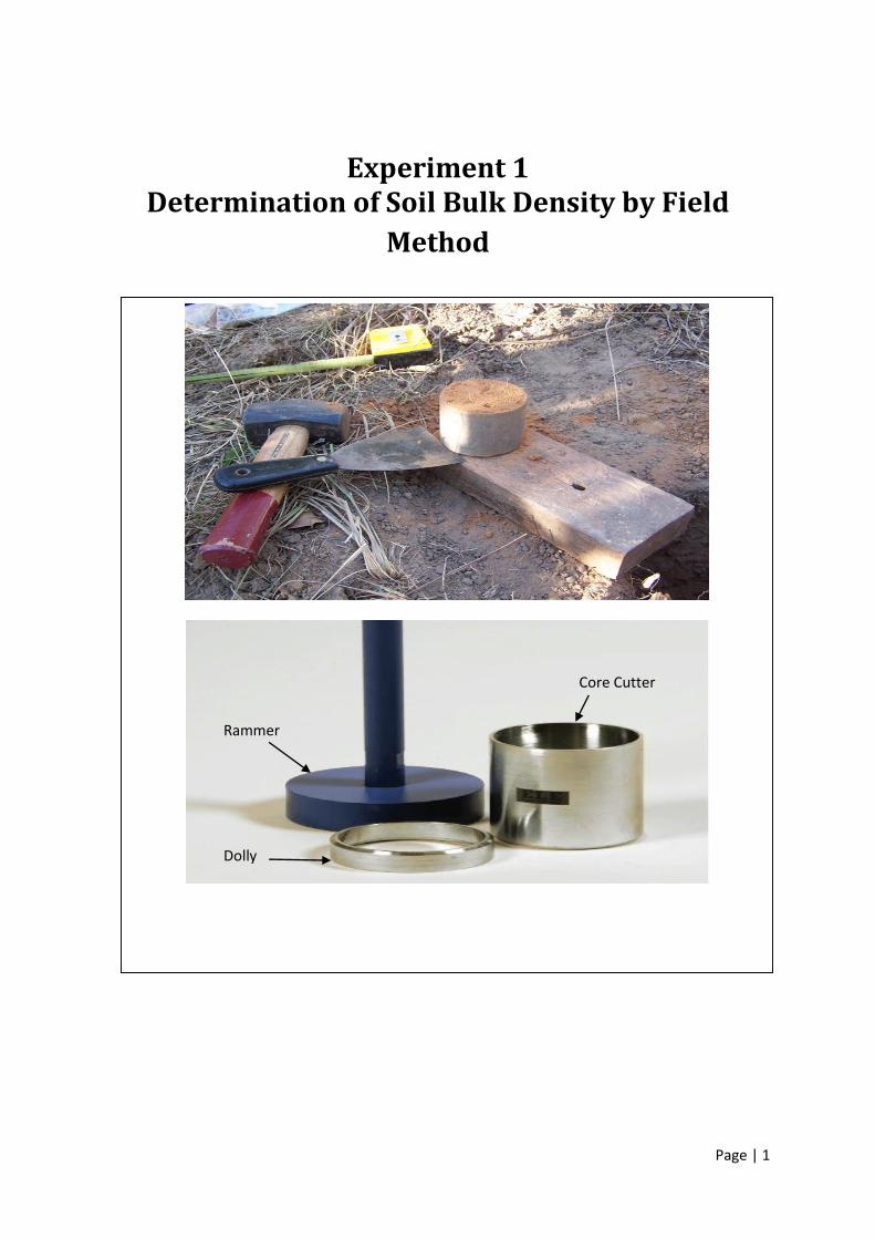
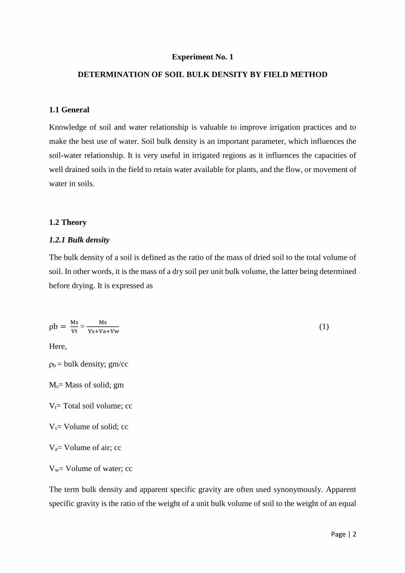
Experiment 1 Determination of Soil Bulk Density by Field
Method
Core Cutter
Rammer
Dolly
Page | 2
Experiment No. 1
DETERMINATION OF SOIL BULK DENSITY BY FIELD METHOD
1.1 General
Knowledge of soil and water relationship is valuable to improve irrigation practices and to
make the best use of water. Soil bulk density is an important parameter, which influences the
soil-water relationship. It is very useful in irrigated regions as it influences the capacities of
well drained soils in the field to retain water available for plants, and the flow, or movement of
water in soils.
1.2 Theory
1.2.1 Bulk density
The bulk density of a soil is defined as the ratio of the mass of dried soil to the total volume of
soil. In other words, it is the mass of a dry soil per unit bulk volume, the latter being determined
before drying. It is expressed as
ρb = Ms
Vt =
Ms
Vs+Va+Vw (1)
Here,
ρb = bulk density; gm/cc
Ms= Mass of solid; gm
Vt= Total soil volume; cc
Vs= Volume of solid; cc
Va= Volume of air; cc
Vw= Volume of water; cc
The term bulk density and apparent specific gravity are often used synonymously. Apparent
specific gravity is the ratio of the weight of a unit bulk volume of soil to the weight of an equal
Page | 3
volume of water. However, since, 1gm of water fills a volume of 1 cc at normal temperatures;
the two terms have equal numerical value.
1.3 Scope of the Test
Bulk density is an important soil physical property considering its influence on the water
holding capacity and hydraulic conductivity of soil. It is influenced by the structure, texture
and compactness of the soil. The bulk density of uncultivated soils usually varies between 1.0
and 1.6; however compact layers may have a bulk density of 1.7 to 1.8. When working with
the irrigated soils, it is necessary to know their bulk density in order to account for the water
applied in irrigation, since it is impractical to measure, by direct means, the volume of water,
which exists in the form of soil moisture in a given volume of soil. It is necessary to measure
the weight of water in a given weight of soil by observing the loss of weight in drying and then
convert the weight percentage so obtained to a volume percentage by use of the bulk density;
thus, the volume of water in a given volume of soil may be determined. From this data the
additional requirement of water in volumetric basis may also be calculated.
1.4 Objective
1) To determine the bulk density of soil.
2) To plot moisture content by weight and moisture content by volume and then determine the
soil bulk density from the graph.
1.5 Procedure
1) The usual method of determining the bulk density or apparent specific gravity of a soil is to
obtain an uncompacted soil sample of known volume. Core samplers are commonly used for
this purpose. The sampler that has a cutting core is driven into the soil and an uncompacted
core obtained within the tube.
2) The samples are carefully trimmed at both ends of the cylinder.
Page | 4
3) They are dried in an oven at 105°C-110°C for about 24 hours until the moisture is driven off
and the sample is then weighted. The volume of a soil core is the same as the inside volume of
the core cylinder.
4) The weight of the soil in grams divided by the volume of soil core in cc is the bulk density
of soil.
5) From the data, calculate moisture content by weight.
6) Find moisture content by volume by multiplying the m/c by weight with bulk density.
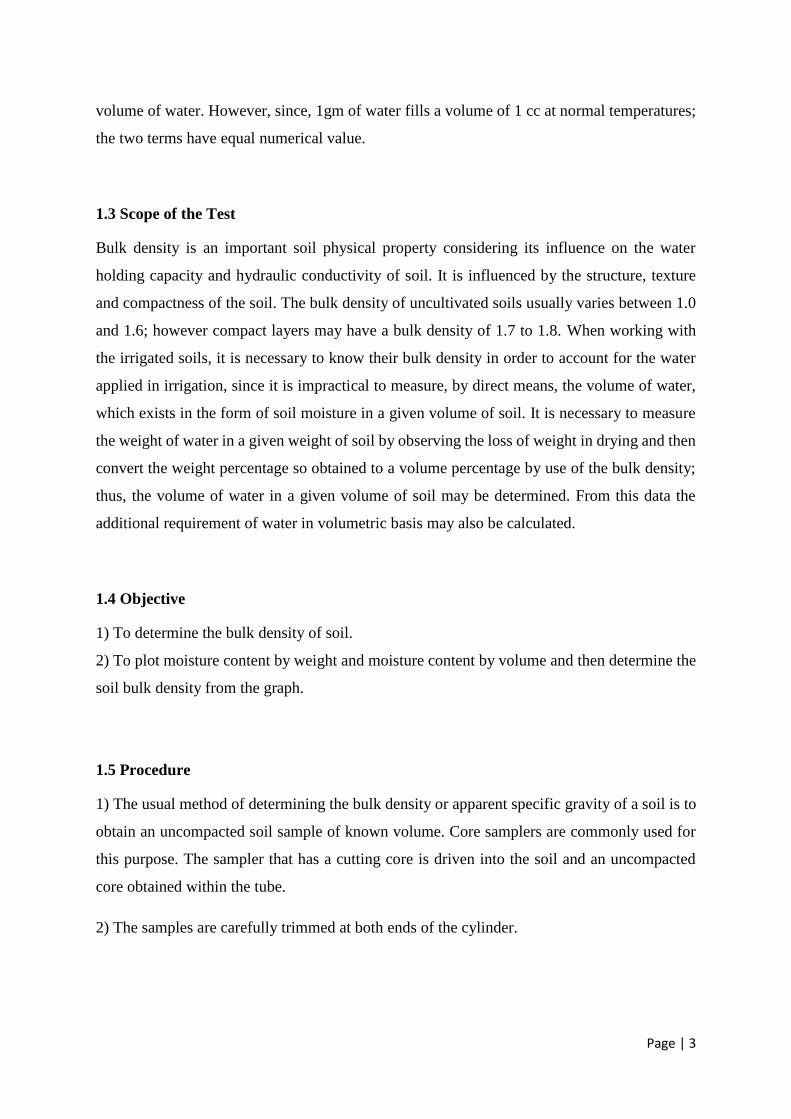
1.6 Qualitative Curve
Figure.1: Moisture content by volume Vs moisture content by weight
1.7 Assignment
1) Prove that ρb= ρs (1-n/100)
ρb= ρs (1+e)
Where, ρs= density of soil, n = porosity,e= void ratio
2) Prove that moisture content by volume is the product of moisture content by weight and bulk
density.
3) “Soil with high bulk density will have low hydraulic conductivity”—explain.
STUDENT ID: DATE:
Page | 5
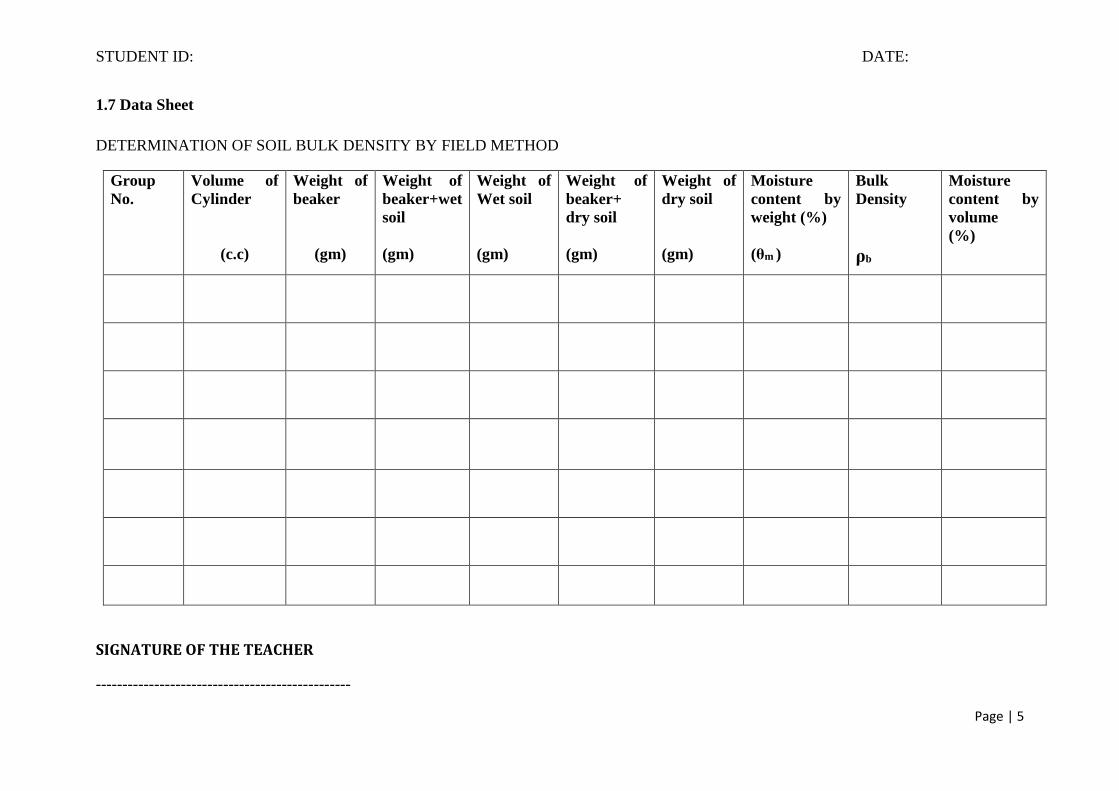
1.7 Data Sheet
DETERMINATION OF SOIL BULK DENSITY BY FIELD METHOD
Group
No.
Volume of
Cylinder
(c.c)
Weight of
beaker
(gm)
Weight of
beaker+wet
soil
(gm)
Weight of
Wet soil
(gm)
Weight of
beaker+
dry soil
(gm)
Weight of
dry soil
(gm)
Moisture
content by
weight (%)
(θm )
Bulk
Density
ρb
Moisture
content by
volume
(%)
SIGNATURE OF THE TEACHER
------------------------------------------------
Page | 6
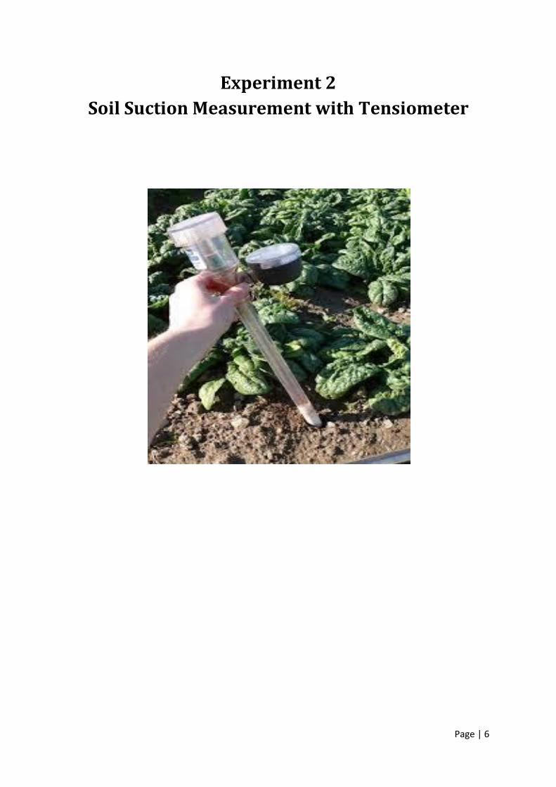
Experiment 2
Soil Suction Measurement with Tensiometer
Page | 7
Experiment No: 2
SOIL SUCTION MEASUREMENT WITH TENSIOMETER
2.1 General
The functions of soil moisture in plant growth are very important. Particularly in irrigated
regions the soil moisture condition is of special interest and importance, because the depth of
water to apply in irrigation and the interval between irrigations are both influenced by present
moisture condition and use rate of applied water. Soil suction measurement with tensiometer
at various time intervals is an indirect mean of measuring soil moisture in the soil.
2.2 Theory
2.2.1 Soil Suction
In unsaturated soils, water is held in the soil matrix under negative pressure due to attraction
of the soil matrix for water. Instead of referring to this negative pressure the water is said to be
subjected to a tension exerted by the soil matrix. The tension with which the water is held in
unsaturated soil is termed as soil-moisture suction or soil-moisture tension.
2.2.2 Tensiometer
The tensiometer is a mechanical device for measuring soil- water tension in the field. The
essential parts of a tensiometer consist of the porous cup with a reservoir of water inside, the
connecting tube, and the sensing element of a vacuum gauge or a mercury manometer.
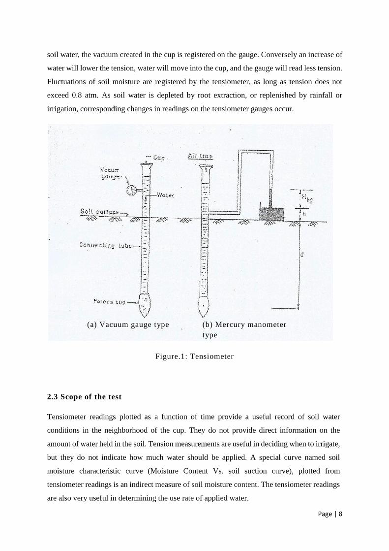
The figure 1 below shows the essential parts of a tensiometer. A porous ceramic cup is
positioned in the soil where information regarding soil water is desired. The cup, the connecting
tube, and the sensing element of a vacuum indicator are all filled with water. Water in the soil
near the cup is in hydraulic contact with bulk water inside the cup through pores in the cup
wall. Flow, in or out through the cup wall, tends to bring the cup water into hydraulic
equilibrium with the soil water. As water moves out of the cup because of the suction in the
Page | 8
soil water, the vacuum created in the cup is registered on the gauge. Conversely an increase of
water will lower the tension, water will move into the cup, and the gauge will read less tension.
Fluctuations of soil moisture are registered by the tensiometer, as long as tension does not
exceed 0.8 atm. As soil water is depleted by root extraction, or replenished by rainfall or
irrigation, corresponding changes in readings on the tensiometer gauges occur.
Figure.1: Tensiometer
2.3 Scope of the test
Tensiometer readings plotted as a function of time provide a useful record of soil water
conditions in the neighborhood of the cup. They do not provide direct information on the
amount of water held in the soil. Tension measurements are useful in deciding when to irrigate,
but they do not indicate how much water should be applied. A special curve named soil
moisture characteristic curve (Moisture Content Vs. soil suction curve), plotted from
tensiometer readings is an indirect measure of soil moisture content. The tensiometer readings
are also very useful in determining the use rate of applied water.
(a) Vacuum gauge type (b) Mercury manometer
type
Page | 9
2.4. Limitation of Tensiometer
Tensiometer does have a definite limitation in the range of values they can measure. The
practical limit is about 0.8 atm. At this pressure air enters the closed system through the pores
of the cup and makes the unit inoperative. The air entry or bubbling pressure of the ceramic
cup limits this range.
2 . 5 O b j e c t i v e
1) Use of tensiometer to measure soil moisture tension.
2) Measure the moisture content of the soil by weight.
3) Plot the soil moisture characteristic curve (moisture content vs. suction).
2 . 6 P r o c e d u r e
1) For field installation, a hole is made in the soil using an auger of diameter larger than the
porous ceramic tube. Insert the porous ceramic tube part in the hole and refill the hole with
the material excavated. The soil surrounding the tensiometer ceramic tube should be
refilled and compacted well to ensure good contact.
2) When suction equilibrium has been reached, take the necessary measurements. For the
laboratory set-up, take tensiometer reading 1 day after installation.
3) Take soil samples from the depth where tensiometer was installed. Determine the weight
of the soil.
4) Put the soil sample in an oven at about 110°C and allow the water to evaporate. The
evaporation process at least takes 24 hours. Determine the weight of the dry soil and the
weight of water.
Page | 10
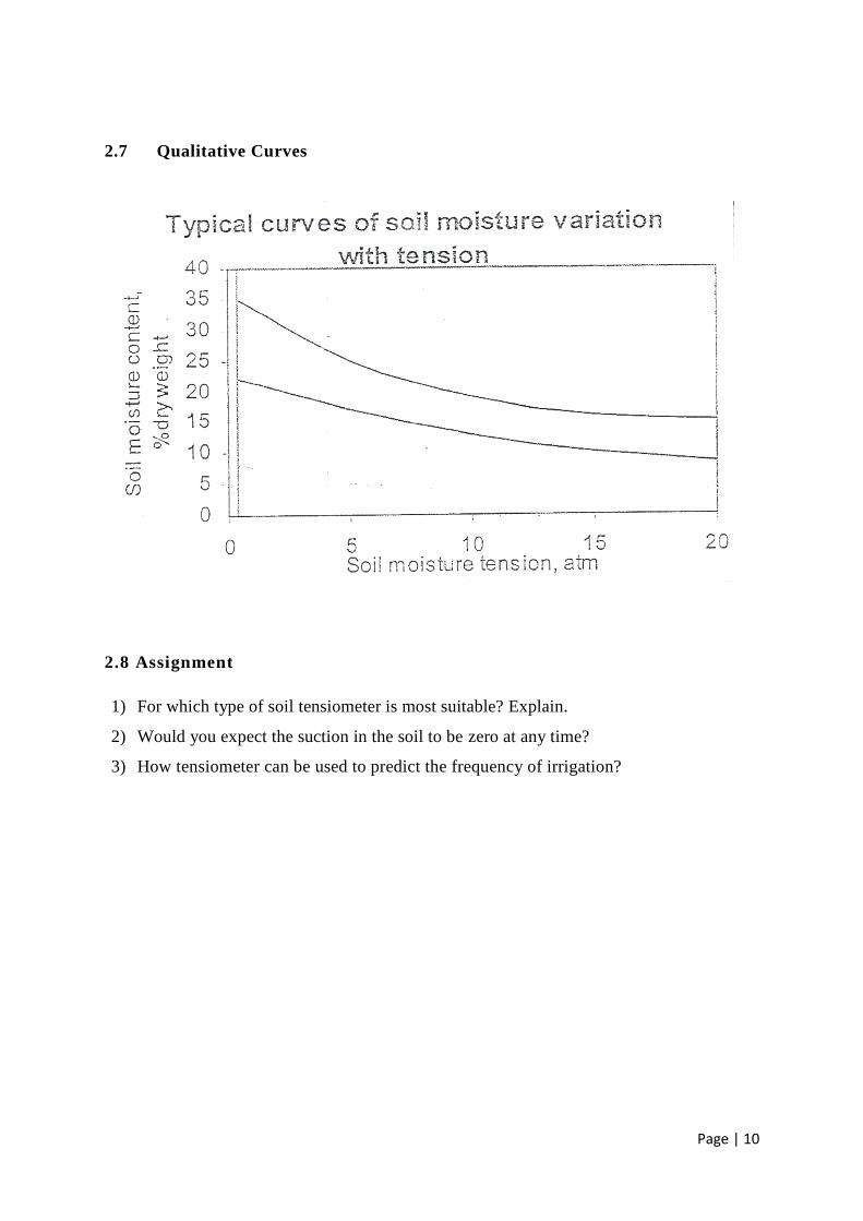
2.7 Qualitative Curves
2.8 Assignment
1) For which type of soil tensiometer is most suitable? Explain.
2) Would you expect the suction in the soil to be zero at any time?
3) How tensiometer can be used to predict the frequency of irrigation?

STUDENT ID: DATE:
Page | 11
2.9 Data Sheet
SIGNATURE OF THE TEACHER
--------------------------------------------------
Group No. Weight of can
(gm)
Weight of wet soil +
can
(gm)
Weight of dry
soil+can
(gm)
Moisture
content (%)
Soil suction
(cm of Hg)
Soil Suction
(atm)
Soil Suction
(centibar)
Page | 12
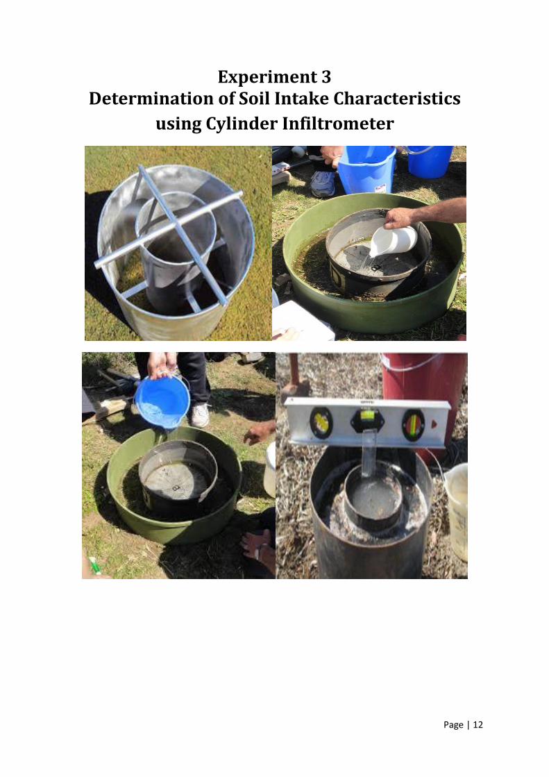
Experiment 3 Determination of Soil Intake Characteristics
using Cylinder Infiltrometer
Page | 13
Experiment No. 3
DETERMINATION OF SOIL INTAKE CHARACTERISTICS USING
CYLINDER INFMTROMETER
3.1 General
Knowledge of the rate of entry of water into soil is of fundamental importance for efficient
irrigation. Soil intake characteristic gives us information about the rate of entry of water into
soil to avoid excess irrigation or shortage of irrigation.
3.2 Theory
3.2.1 Intake rate
The rate of entry of water into soil under field conditions is called intake rate. Whenever the
configuration of soil surface influences the rate of water entry, the term intake rate should be
used rather than the term infiltration rate to refer to the rate of entry of water into soil. Intake
rate is therefore influenced by furrow size, shape as this term indicates infiltration under a
particular soil surface configuration. On the other hand the term "infiltration" applies to a
level surface covered with water.
3.2.2 Scope of the test
In all irrigation methods, except sub-surface irrigation, water is applied to the surface of land
where it subsequently enters the soil and is stored for later use by plants. The object of
irrigation is to get water into the soil where it can be stored. The intake rates obtained from
the tests are indicative of the rates to be expected during irrigation provided, the surface
condition is same. If intake rate is greater than irrigation rate sufficient water will neither
enter the soil nor be stored therein and crop growth is significantly reduced. Again, if
irrigation rate is greater than intake rate, runoff loss will occur. One of the major problems of
irrigated farms is the low intake rate of fine textured soil, which is often reduced further by
excessive working of soil and by salinity. Thus the determination of soil intake characteristic
is of fundamental importance in irrigation practice.
Page | 14
3.2.3 Factors affecting Intake Rate
Intake rate varies with many factors, including depth of water on the surface,
temperature of water and soil, soil structure and texture, moisture content and salinity
of the soil.
Retarding layers of soil will greatly influence the rate.
Configuration of the surface such as furrow shape and size, as well as the method of
application, will be influencing factor also. Hence intake rate varies from place to
place on a field and it also varies with time.
3.3 Method ofdetermining Intake Rate
The best method of determining intake rate is to obtain direct measurements by recording the
water applied less the water flowing from the field. When direct measurements are .not feasible,
cylinder infiltrometers can be used with reasonable accuracy.
3.3.1 Cylinder Infiltrometer
Cylinder infiltrometers have been found suitable for use in determining intake characteristics of
irrigated soil. The cylinders should be at least 25 cm in diameter and 30 cm long. The cylinder
should be carefully driven into the soil to a depth of about 15 cm. To begin a test, about 10 to
12 cm of water is quickly poured into the cylinder and timingof infiltration is recorded. The
water surface readings are made from a datum with the help of a ruler. To represent the soil
intake characteristics it is necessary to plot the accumulated intake vs. time. The equation for
accumulated intake is
D = CTn (1)
Where D = accumulated intake, mm
T = time, min
C and n = constants
Page | 15
Average intake rate is given-by
Iave=𝐷
𝑇 =
CTn
𝑇 = CTn-1 (2)
Instantaneous intake rate is given by
Iins=𝑑𝐷
𝑑𝑇 = CnTn-1 (3)
3.3.2 Double Ring Infiltrometer (Buffer ponds)
After water penetrates to the bottom of the cylinder, it will begin to spread radially and
the rate of intake will change accordingly. When a principal-restricting layer does not
lie within the depth of penetration of the cylinder, the radial flow will cause considerable
change in the intake rate. Buffer ponds surrounding the cylinder are used to minimize
this effect. Buffer ponds can be constructed by forming an earth dike around the cylinder
or by driving a larger diameter cylinder concentric with the intake cylinder into the soil.
The water level in both the cylinders should be equal and approximately the depth to be
expected during the irrigation. Care should be taken not to puddle the soil when water
is added to the cylinder or the buffer pond.
3.4 Objective
1) To familiarize with the field testing procedure.
2) To plot accumulated depth Vs. time in a log-log paper and to find (a) the constant C, and
(b) the exponent, n.
3) To develop the equations for accumulated intake, average and instantaneous intake rates
from the test data.
4) To plot accumulated depth, average and instantaneous intake rate Vs. time in one plain
graph paper.
3.5 Procedure
1) Note the soil profile and surface condition.
2) The cylinder should be carefully driven into the soil to a depth of about 15 cm
Page | 16
3) To begin a test, about 10 to 12 cm of water is quickly poured into the cylinder and timing
of infiltration is recorded.
4) At various time intervals, measure the water level.
5) Calculate the time difference and water level difference.
6) The ratio of water level difference and time difference gives the instantaneous intake
rate at different times.
7) The ratio of cumulative depth and cumulative time gives average intake rate.
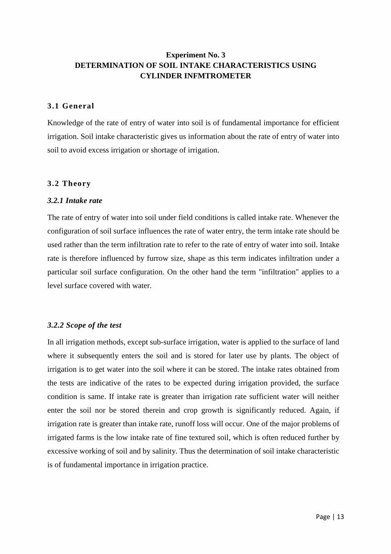
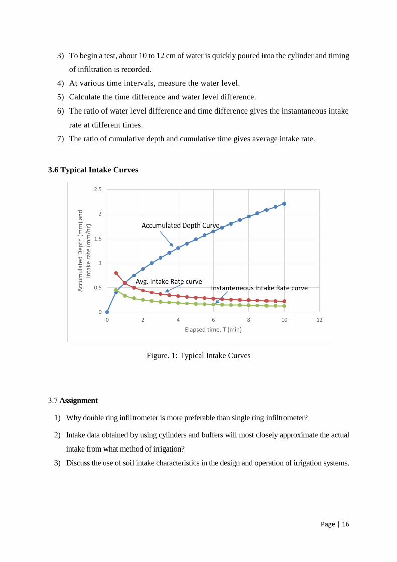
3.6 Typical Intake Curves
Figure. 1: Typical Intake Curves
3.7 Assignment
1) Why double ring infiltrometer is more preferable than single ring infiltrometer?
2) Intake data obtained by using cylinders and buffers will most closely approximate the actual
intake from what method of irrigation?
3) Discuss the use of soil intake characteristics in the design and operation of irrigation systems.
0
0.5
1
1.5
2
2.5
0 2 4 6 8 10 12
Acc
um
ula
ted
Dep
th (
mm
) an
dIn
take
rat
e (m
m/h
r)
Elapsed time, T (min)
Accumulated Depth Curve
Avg. Intake Rate curveInstanteneous Intake Rate curve

Page | 17
STUDENT ID: DATE:
3.8 Data Sheet
DETERMINATION OF SOIL INTAKE CHARACTERISTICS USING CYLINDER
INFILTROMETER
Cylinder No. _______________________Diameter of Cylinder= _____________________
Time, minutes Infiltration, mm Average
Intake
Rate, Iavg
(mm/hr)
Instantaneous
Intake Rate,
Iins
(mm/hr)
Actual
Time
Difference
(min)
Cumulative Difference Depth
(mm)
Cumulative
SIGNATURE OF THE TEACHER
-------------------------------------------------
Page | 18
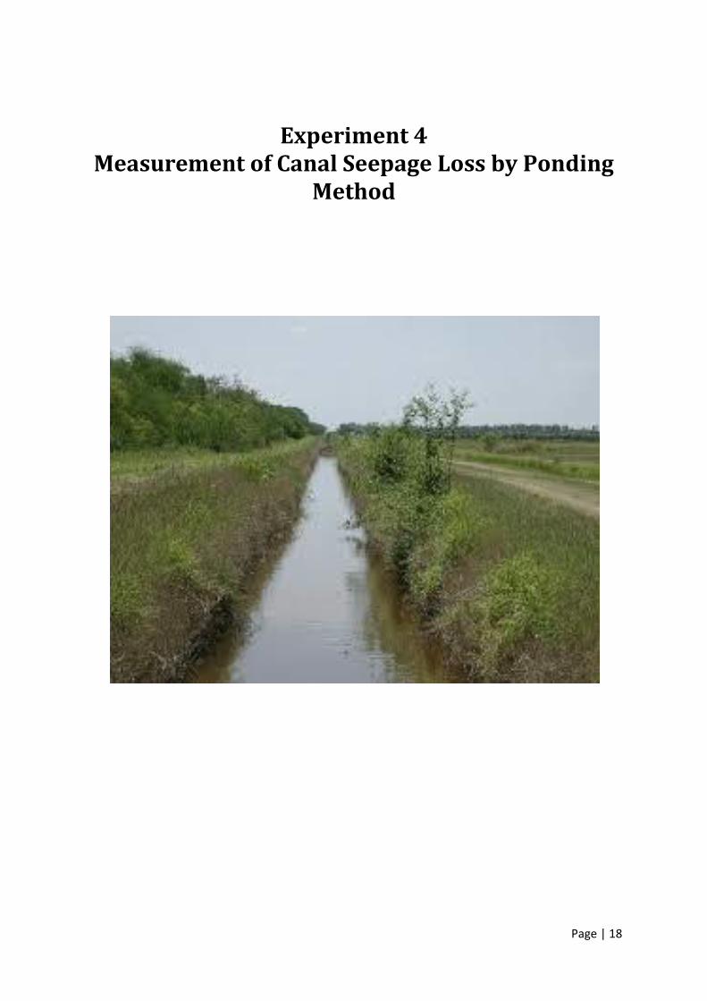
Experiment 4 Measurement of Canal Seepage Loss by Ponding
Method
Page | 19
Experiment No. 4
MEASUREMENT OF CANAL SEEPAGE LOSS BY PONDING METHOD
4.1 General
Determination of canal seepage loss is of very importance to make a provision for water
loss in irrigation canal and to consider the other phenomena associated with canal seepage.
4.2 Theory
4.2.1 Canal Seepage Loss
During the passage of water from the main canal to the outlet at the head of the watercourse,
water may be lost either by evaporation from the surface or by seepage through the peripheries
of the channels. These losses are sometimes very high of the order of 25% to 50% of the water
diverted. Evaporation losses are generally of the order of 2 to 3 percent of the total loss and
may be more but seldom exceed 7%. So the major portion of the total loss is seepage loss
and a minor portion is evaporation loss.
4.3 Scope of the test
In determining the channel capacity a provision, for water loss must be made. In this regard
measurement of seepage loss is very important. Moreover seepage of water from irrigation
canals is a serious problem. Not only is water lost, but also drainage problems are often
aggravated on adjacent or lower lands. Occasionally water that seeps out of canal re-enters the
river valley where it can be rediverted, or enters in an aquifer where it can be reused. It is a
more serious economic loss when the seepage losses are not recoverable. Also economic and
legal problems may result from water seepage from canals causing drainage problems on the
lower lying lands. So determination of canal seepage loss is of very importance to visualize
the total loss as well as the other effects.
Page | 20
4.4 Factors affecting Canal Seepage Loss
Type of seepage, i.e. whether "percolation" or absorption.
Soil permeability.
The condition of the canal. The seepage through a silted canal is less than that from a
new canal.
Amount of silt carried by the canal; the more the silt, the lesser are the losses.
Velocity of canal water; the more the velocity, the lesser will be the losses.
Cross-section of the canal and its wetted perimeter.
4.5 Methods of determining Canal Seepage Loss
Several methods used to measure seepage from canals are inflow-outflow, ponding method,
seepage meters, laboratory tests of permeability of soil etc.
4.5.1 Ponding methods
The ponding measurements are well adapted to estimate the seepage loss in short canal sections.
The measurement can be made by installing a check or a dam at both ends of a canal section,
filling the section with water and observing the rate at which the water level recedes with time.
The recession rate can be determined by plotting the water level against time and noting the
slope of the resulting curve at the operating level. The seepage rate is computed as
S= 𝑅𝑊𝐿
𝑃𝐿 (1)
Where, S= seepage rate, m/day
R = Rate of recession or slope of water level versus elapsed time curve at operating
level, m/day
W = Average top width of the water surface, m
P = Average wetted perimeter of the test section, m
L = Length of the test section, m
Page | 21
4.6 Objective
1) To get acquainted with the field testing procedure
2) To estimate the seepage loss in the test canal section
3) Interpretation of the test results.
4.7 Procedure
1) At first construct a dam or check at the both ends of a short reach of the canal.
2) Fill the section with water
3) Observe the rate at which the water level recedes with time.
4) Plot the water level against time
5) Find the slope of resulting curve at operating level. The value of the slope is called
recession constant.
6) Determine channel seepage loss using equation (1).
4.8 Assignment
1) What are the advantages and disadvantages of ponding method?
2) What is the difference between canal seepage loss and canal conveyance loss? How
can you reduce the canal seepage loss?

Page | 22
STUDENT ID: DATE:
4.8 Data Sheet
MEASUREMENT OF CANAL SEEPAGE LOSS BY PONDING METHOD
A. Test Section Characterization
Canal: _________________________ Section No: ______________________________
Soil Type: ______________________ Canal condition: ___________________________
Section Length: _________________ Operating Level: ___________________________
B. Cross-sectional Profile:
Cross section 1 Cross section 2 Cross section 3
W= _______________ W= ______________ W= ______________
Average width, w= ________________________
C. Recession
Time
Scale Reading
Water Level
(mm) Actual time Difference(min) Cumulative
SIGNATURE OF THE TEACHER
----------------------------------------------------
Page | 23
Experiment 5 Abstraction from a Single Well in an Unconfined
Aquifer
Page | 24
Experiment No. 5
ABSTRACTION FROM A SINGLE WELL IN AN UNCONFINED AQUIFER
5 .1 General
Efficient and economical utilization of ground water through wells depends on the
design of wells to best suit the characteristics of the water bearing formation. Flow of
ground water into wells is influenced by the physical characteristics of the water
bearing formations, the number and extent of these formations, the elements of well design
and the methods used for constructing and developing the wells.
5.2Theory
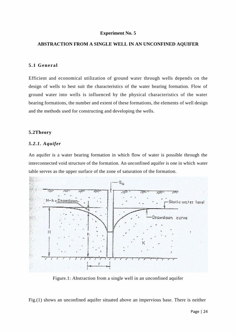
5.2.1. Aquifer
An aquifer is a water bearing formation in which flow of water is possible through the
interconnected void structure of the formation. An unconfined aquifer is one in which water
table serves as the upper surface of the zone of saturation of the formation.
Figure.1: Abstraction from a single well in an unconfined aquifer
Fig.(1) shows an unconfined aquifer situated above an impervious base. There is neither
Page | 25
recharge by rainfall, nor loss of water due to evapotranspiration. Initially, the water table is
horizontal. Abstraction of water from a well results in lowering of water table around the
well, and then there is a reduction of the saturated thickness of the well.
5.2.2 Prediction of well yield
Irrigation wells operate according to certain fundamental hydraulic principles. Water flows
into the well from the surrounding aquifer because the pumping of the well creates a
difference in pressure. Darcy's theory established the fundamentals of ground water
movement. Dupuit, a French hydraulic engineer established the analysis of seepage
phenomenon and derived the well equations based on the following assumptions:
i) The hydraulic gradient is the same at all points in a vertical section of an aquifer.
ii) The hydraulic gradient at the water table (or at the piezometric surface in artesian flow)
is equal to the slope of the surface at that point.
The equation of flow, for unconfined aquifer becomes:
From Dercy's Law:
Q= kiA = 2nrh K dh/dr (1)
From Continuity Principle:
Q=Constant= Q0 (2)
Combining (1) and (2) and integrating gives Dupuit formula
𝐻2 − ℎ2 =𝑄0
𝜋𝐾𝑙𝑛
𝑅0
𝑟 (3)
Where,
H = depth of saturated thickness before pumping
h = depth of saturated zone at a distance 'r'
Qo = well discharge
Ro = radius of influence
K = coefficient of permeability
H-h = s
= drawdown
Page | 26
If s<<H, then H+h ~2H and equation 3 can be written as
𝑠 =𝑄0
2𝜋𝑇𝑙𝑛
𝑅0
𝑟 (4)
Where, T = KH, the coefficient of transmissibility. Changing the base of logarithm, we get
Thiems equation
𝑠 =2.303𝑄0
2𝜋𝑇𝑙𝑛
𝑅0
𝑟 (5)
5.3 Scope of the test
Irrigation wells are usually designed to obtain the' highest yield available from the aquifer,
and the highest efficiency in terms of specific capacity. The yield potential of a well is
evaluated on the basis of hydrological conditions of the area- rainfall, runoff and recharge.
When the yield potential of an area is not a limiting factor a properly designed irrigation well
should provide the required quantity of water to irrigate the entire area owned by the farmer.
So determination of yield potential of a well is very useful.
The topography of the farm, current water table condition, recharge possibilities etc are
important factors in deciding the location of a well. The draw down curves and the water table
contour can be helpful in this regard.
Whenever a well is pumped, the greatest amount of lowering of the water table occurs within
the well and the immediately adjacent areas are lowered almost as much. But as pumping
continues, a equilibrium gradient is established and the quantity of water entering the well
from the surrounding zone will be approximately the same as that being pumped. The amount
of lowering diminishes as the distance from the well increases, until a point is reached where
pumping does not affect the level of the overall water table. If wells are spaced too closely
together, the pumping of one may interfere with the yield of others. In other words, the yield
of a well is decreased if its cone of depression is overlapped by the cone of an adjacent well.
To select the suitable spacing we may take the help of the value of radius of influence.
Experience and tests have shown that, in most cases, grouping of well should not be made at
interval less than 70 meters.
Page | 27
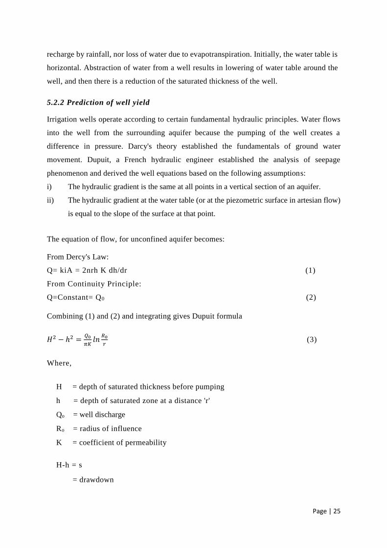
5.4 Efficiency of a Well
The discharge from well is approximately proportional to the drawdown s. The discharge
per unit drawdown is called the specific capacity of the well. This specific capacity will
be different for different well designs. For determining the best draw down-discharge
conditions for a well, the well may be operated under varying drawdown conditions, and
then a graph may be plotted between discharge and drawdown (called yield-draw down
curve).
The curve obtained is a straight line up to a certain stage of drawdown, beyond which the
drawdown increases disproportionately with yield. This places an optimum and efficient limit
to be created in a well. This is generally found to be 70% of maximum drawdown, which can
be created in a well.
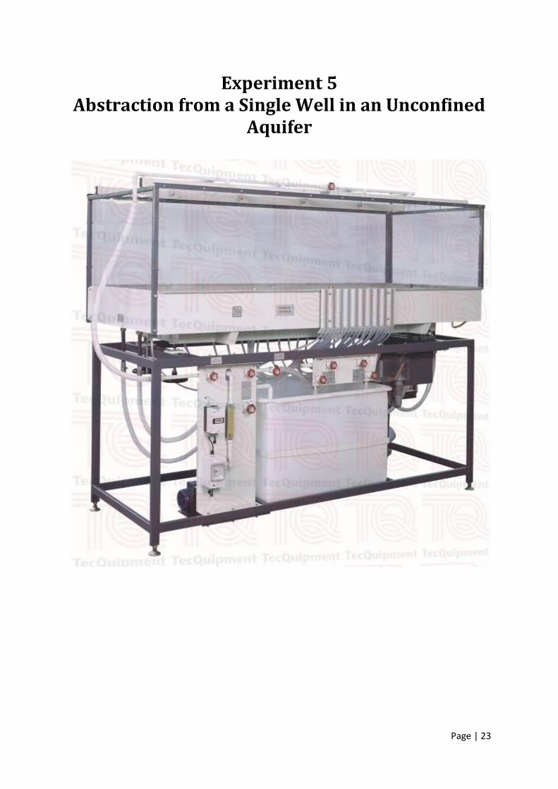
5.5 Description of the Apparatus
The experiment will be carried out in the 'Basic Hydrology System', which consists of a
catchment basin, represented by a shallow tank filled with sand. At the two longitudinal ends
of the catchment there are two submergence tanks, each connected by a water inlet pipe and
Page | 28
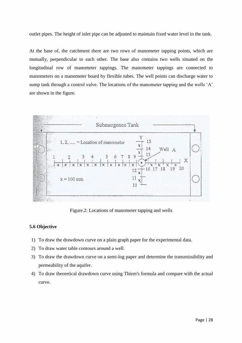
outlet pipes. The height of inlet pipe can be adjusted to maintain fixed water level in the tank.
At the base of, the catchment there are two rows of manometer tapping points, which are
mutually, perpendicular to each other. The base also contains two wells situated on the
longitudinal row of manometer tappings. The manometer tappings are connected to
manometers on a manometer board by flexible tubes. The well points can discharge water to
sump tank through a control valve. The locations of the manometer tapping and the wells ‘A’
are shown in the figure.
Figure.2: Locations of manometer tapping and wells
5.6 Objective
1) To draw the drawdown curve on a plain graph paper for the experimental data.
2) To draw water table contours around a well.
3) To draw the drawdown curve on a semi-log paper and determine the transmissibility and
permeability of the aquifer.
4) To draw theoretical drawdown curve using Thiem's formula and compare with the actual
curve.
Page | 29
5.7 Procedure of Experiment
1) Keeping the well discharge valve closed, flood the catchment to make the sand
completely saturated.
2) Adjust the two groundwater inlet pipes to the same level, to maintain fixed water levels
in the submergence tank.
3) Adjust the discharge to a valve suitable for the experiment and wait till water levels in
all the manometers stand at the same height, and note the water levels in manometer.
4) Open the well discharge valve, and wait until water levels in all the manometers become
stable.
5) Connect the well discharge pipe to a measuring tank and measure the well discharge.
6) Note the water levels in the manometers no. 5 through 20.
5.8 Assignment
1) Distinguish between (1) confined and unconfined aquifers; (ii) static water level and
pumping water level; (iii) specific capacity and specific yield; (iv) co-efficients of
permeability and transmissibility.
2) Discuss the effect of partial penetration of well. (Hints: Irrigation theory and practice
by A M Michael)
3) What are the effects of well size and radius of influence on well yield in context to
environmental considerations and economy? (Hints: Irrigation theory and practice by
A M Michael)
Page | 30
STUDENT ID: DATE:
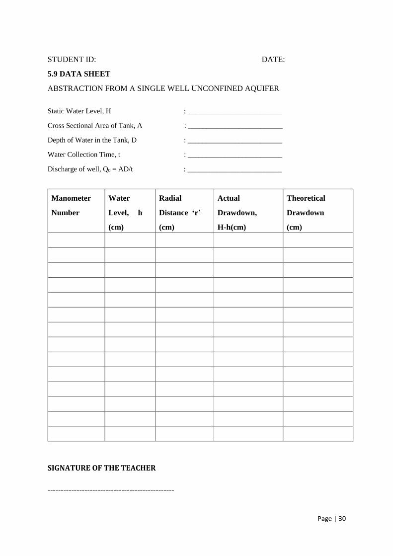
5.9 DATA SHEET
ABSTRACTION FROM A SINGLE WELL UNCONFINED AQUIFER
Static Water Level, H : __________________________
Cross Sectional Area of Tank, A : __________________________
Depth of Water in the Tank, D : __________________________
Water Collection Time, t : __________________________
Discharge of well, Q0 = AD/t : __________________________
Manometer
Number
Water
Level, h
(cm)
Radial
Distance ‘r’
(cm)
Actual
Drawdown,
H-h(cm)
Theoretical
Drawdown
(cm)
SIGNATURE OF THE TEACHER
------------------------------------------------
Page | 31
Experiment No. 6
IRRIGATION SCHEDULING BY BOOK KEEPING
METHOD
Page | 32
Experiment No. 6
IRRIGATION SCHEDULING BY BOOK KEEPING METHOD
6.1 General
The knowledge of irrigation scheduling, total water requirement and irrigation requirement
is fundamental in the design of irrigation scheme and water supply system and in irrigated
crop production.
6.2 Theory
6.2.1. Irrigation Scheduling
Irrigation scheduling is a decision making process involving when to irrigate, how much water
to apply each time and how to apply. In other words scheduling of irrigation refers to
application of water at the right time in the right amount by the right method.
6.2.2. Necessity of Irrigation Scheduling
The main objective of irrigation scheduling is management of water so that it is applied at
right time and in the amount needed. In water short areas this can result in increased yields
through an extension of cropped areas. In water surplus areas it can help to alleviate problems
which may result from excess water applications. It can also reduce loss of nutrients through
deep percolation.
6.2.3. Dependable Factors
An efficient and accurate irrigation-scheduling program depends on the following
information of that area:
Soil information
Crop information
Meteorological information
Water supply information
Methods of irrigation
Social & economic factors
Page | 33
Two basic information that must be known before irrigation scheduling are:
Soil moisture available for crop
Rate of daily water use by the crop
6.2.4. Irrigation Scheduling by Book Keeping Method
In this method a worksheet for "Moisture balance for scheduling irrigation" is used for weekly
or daily basis. Before starting this scheduling three major items should be known:
Water holding capacity (WHC) of soil in the root depth
Estimated Etc of the crop to be grown
Soil moisture balance at the beginning of the scheduling period
By entering all these in the appropriate column of the worksheet the moisture balance at the
end of the week is determined.
6.2.5 Field Capacity (FC)
Yield capacity is the moisture content of the soil when rapid drainage has essentially ceased
and any farther drainage occurs at a very slow rate. The FC corresponds to a soil moisture
tension of about 1/10 to 1/3 atmosphere.
6.2.6. Permanent Wilting Point (PWP)
The Soil moisture content at which the plant wilts permanently or dies is known as permanent
wilting point. The soil still contains some water but it is too difficult for the roots to extract
it from the soil as it is held with a suction force of about 15 atm. Typically for medium soils
the moisture content at PWP is about one-half the FC.
6.2.7. Gravitational Water
The water in the large pores that moves downward freely under the influence of gravity is known
as the. gravitational water. This is the water between the saturated point and FC.
6.2.8. Available Water
The water contained in the, soil between FC and PWP is known as the available water.
6.2.9. Total Available Water (TAW)
The amount of water, which will be available for plants in the root zone, is known as the total
available water. It is the difference in volumetric moisture content at FC and at PWP;
multiplied-by root zone depth.
Page | 34
6.2.10. Management Allowable Depletion (MAD)
MAD is the degree, to which the water in the soil is allowed to be depleted by management
decision.
6.2.11. Reference Crop Evapotransporation (ETo)
The rate of evapotranspiration from an extensive surface of 8 to 15 cm tall green grass cover
of uniform height, actively growing, completely shading the ground and of not short of water
is known as the reference crop evapotranspiration.
6.2.12. Crop Evapotranspiration (ETc)
The depth of water needed to meet the water loss through evapotranspiration of a disease-
free crop, growing in large fields under non-restricting soil conditions including water and
fertility and achieving full production potential under-the given growing environment.
6.2.13. Crop Coefficient (Kc)
The ratio of ETc / ETo is termed as crop coefficient.
6.2.14. Effective Rainfall (Re)
Rain that is retained in the root zone and used by plants is considered as effective rainfall.
Effective Rainfall (Re) =Total rainfall(R)-Runoff (R0)-Evaporation (E)-Deep
percolation (P)
6.3 Procedure
1) To calculate the WHC of soil in the root zone depth the m/c at PWP is subtracted from
m/c at FC then multiplied by root zone depth
(𝐹𝐶 − 𝑃𝑊𝑃)
100∗ 𝐴𝑠 ∗ 𝑅𝐷
2) This available water is multiplied by an allowable depletion factor to determine the
allowable depletion.
3) To calculate the current depletion (CD) the actual evapotranspiration and previous
depletion is added and actual rainfall & irrigation (if any applied in the previous week)
is subtracted from the previous sum.
Page | 35
CD = (ETa + previous depletion)-(actual rainfall + irrigation)
4) To calculate the predicted evapotranspiration Kc is multiplied by reference crop
evapotranspiration.
5) The predicted depletion is calculated by adding the predicted evapotranspiration and
current depletion and then subtract the rainfall from it. This predicted depletion is the
amount for irrigation.
6) The irrigation frequency is calculated by using the following expression
Irrigation frequency = 7*(Allowable depletion-CD+R)/Etc
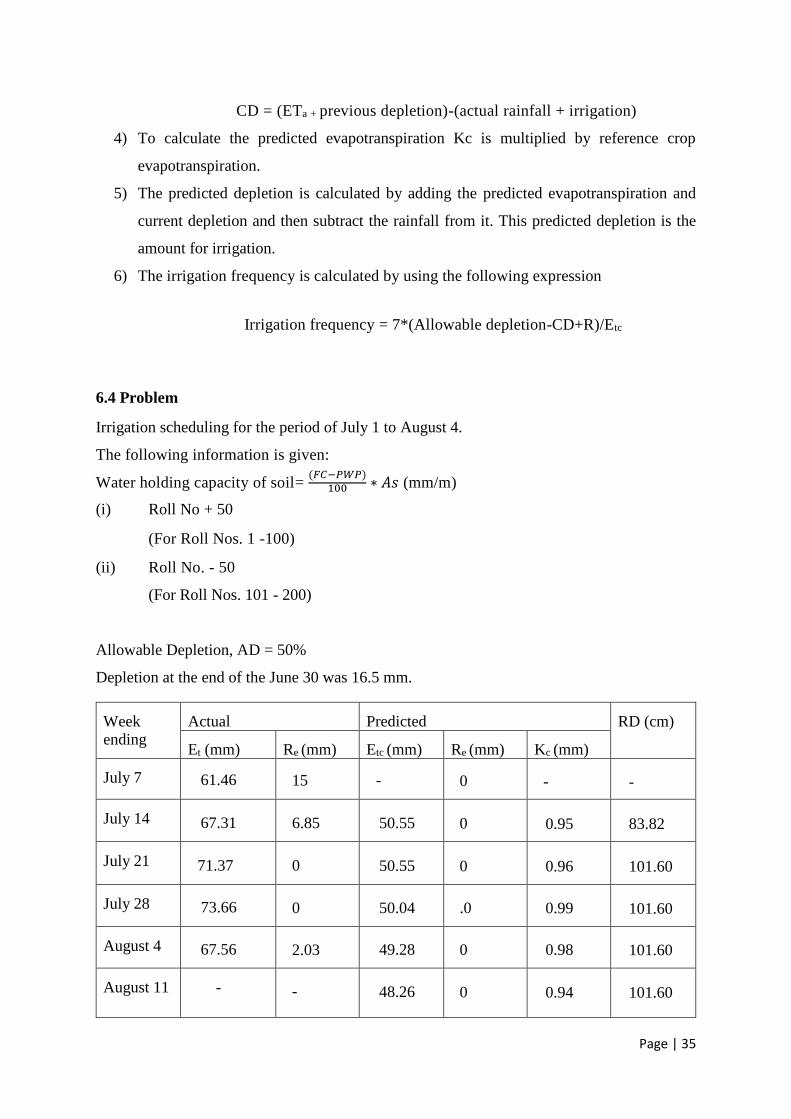
6.4 Problem
Irrigation scheduling for the period of July 1 to August 4.
The following information is given:
Water holding capacity of soil= (𝐹𝐶−𝑃𝑊𝑃)
100 ∗ 𝐴𝑠 (mm/m)
(i) Roll No + 50
(For Roll Nos. 1 -100)
(ii) Roll No. - 50
(For Roll Nos. 101 - 200)
Allowable Depletion, AD = 50%
Depletion at the end of the June 30 was 16.5 mm.
Week ending
Actual Predicted RD (cm)
Et (mm) Re (mm) Etc (mm) Re (mm) Kc (mm)
July 7 61.46 15 - 0 - -
July 14 67.31 6.85 50.55 0 0.95 83.82
July 21 71.37 0 50.55 0 0.96 101.60
July 28 73.66 0 50.04 .0 0.99 101.60
August 4 67.56 2.03 49.28 0 0.98 101.60
August 11 - - 48.26 0 0.94 101.60

Page | 36
6.5Assignment
1) Explain why soil, climate and crop factors are considered while designing irrigation
frequency.
2) "Shallow rooted crops will require more frequent irrigation than deep rooted crops" --
- explain.
3) How can you apply this method in improving the water management practice?
4) What modifications do you need to. apply this method for scheduling irrigation of
rice?

STUDENT ID: DATE:
Page | 37
Data Sheet
IRRIGATION SCHEDUALING BY HAND CALCULATOR METHOD
Calculation Sheet
PREVIOUS WEEK SOIL WATER
BUDGET
IRRIGATION PREDICTION NEXT 7 DAYS
Week
Ending
Etc
Actual
mm
Previous
Deple-
tion+ Etc
mm
Rain
Actual
+
Irrigat-
ion
mm
Current
Depleti-
on CD
mm
Next 7
Days
Etc=Etr
xKc
mm
Root
Dept
h
RD
mm
Water
Holding
Capacity
HC
mm/m
Available
Water
AW =
RDxHC
mm
Allowable
Depletion
AD %
Allowable
Depletion
ADI=
AWx AD
mm
Expected
Effective
Rainfall
Re
mm
Predicted
Depletion
Etc+CD-Re
mm
Days to
Next
Irrigation
= 7(ADI-
CD+Re)/
Etc
Comment
SIGNATURE OF THE TEACHER
----------------------------------------------------
Page | 38
Experiment No. 7
DESIGN OF A BRANCH CANAL IN AN IRRIGATION
PROJECT
Page | 39
Experiment No. 7
DESIGN OF A BRANCH CANAL IN AN IRRIGATION PROJECT
7.1 General
In irrigation project a branch canal is needed to convey water from main canal to the tertiary
canal.
7.2 Theory
7.2.1. Regime Channels
A channel is said to be in a state of regime if there is neither silting nor scouring in the
channel. The shape, longitudinal slope, cross sectional dimension of a regime channel
depends on the discharge, the sediment size, and sediment load. Two approaches of regime
channel design are:
1. Kennedy's approach
2. Lacey’s approach
In Kennedy and Lacey's approach the channel should be trapezoidal with side slope ½ H : 1 V
7.2.2. Kennedy’s Approach
If the velocity in channel is sufficient to keep the sediment is suspension then silting in the
channel will be avoided. Kennedy defined the critical velocity (V0) as the mean velocity
in a channel, which will just keep the channel free from silting& scouring.
7.2.3. Lacey's Approach
Lacey found many drawbacks in Kennedy's theory & put forward his new theory. Kennedy
stated that a channel is said to be in a regime state if there is no silting &nor scouring. Lacey
stated that a channel showing no silting & non-scouring might not be in regime. According to
Lacey a channel is in true regime only if the following conditions are satisfied.
Discharge is constant
Flow is uniform
Silt charge is constant; i.e. the amount of silt is constant
Silt grade is constant; i.e. the type & size of silt is always same
Page | 40
Channel is flowing through a material which can be scoured as easily as it can be
deposited (such soil is known as incoherent alluvium) & is of the same grade as
is transported.
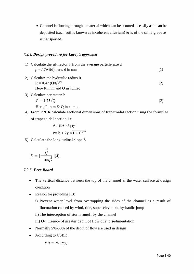
7.2.4. Design procedure for Lacey’s approach
1) Calculate the silt factor fs from the average particle size d
fs =1.76√(d) here, d in mm (1)
2) Calculate the hydraulic radius R
R = 0.47 (Q/fs)1/3 (2)
Here R in m and Q in cumec
3) Calculate perimeter P
P = 4.75√Q (3)
Here, P in m & Q in cumec
4) From P & R calculate sectional dimensions of trapezoidal section using the formulae
of trapezoidal section i.e.
A= (b+0.5y)y
P= b + 2y √1 + 0.52
5) Calculate the longitudinal slope S
𝑆 = [𝑓𝑠
53
3340𝑄16
](4)
7.2.5. Free Board
The vertical distance between the top of the channel & the water surface at design
condition
Reason for providing FB:
i) Prevent water level from overtopping the sides of the channel as a result of
fluctuation caused by wind, tide, super elevation, hydraulic jump
ii) The interception of storm runoff by the channel
iii) Occurrence of greater depth of flow due to sedimentation
Normally 5%-30% of the depth of flow are used in design
According to USBR
FB = √(c*y)
Page | 41
Here, c=coefficient
=1.5 for discharge Q<20 cfs
=2.5 for discharge Q>300cfs
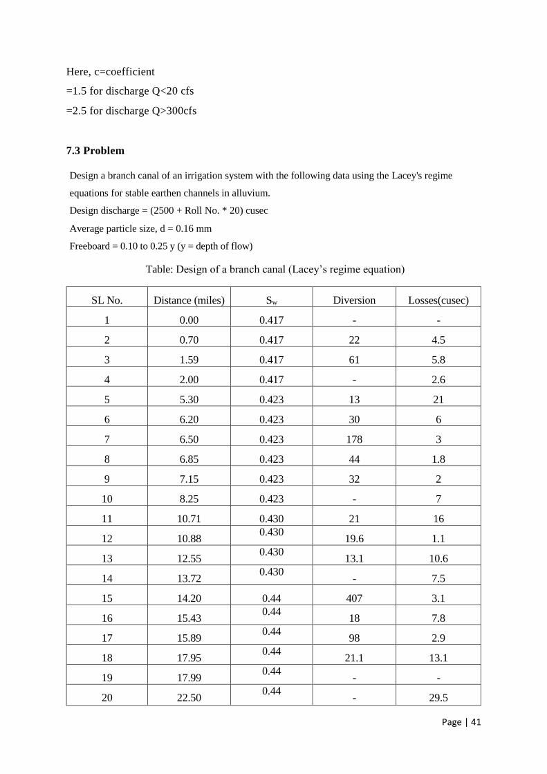
7.3 Problem
Design a branch canal of an irrigation system with the following data using the Lacey's regime
equations for stable earthen channels in alluvium.
Design discharge = (2500 + Roll No. * 20) cusec
Average particle size, d = 0.16 mm
Freeboard = 0.10 to 0.25 y (y = depth of flow)
Table: Design of a branch canal (Lacey’s regime equation)
SL No. Distance (miles) Sw Diversion
(cusec)
Losses(cusec)
1 0.00 0.417 - -
2 0.70 0.417 22 4.5
3 1.59 0.417 61 5.8
4 2.00 0.417 - 2.6
5 5.30 0.423 13 21
6 6.20 0.423 30 6
7 6.50 0.423 178 3
8 6.85 0.423 44 1.8
9 7.15 0.423 32 2
10 8.25 0.423 - 7
11 10.71 0.430 21 16
12 10.88 0.430
19.6 1.1
13 12.55 0.430
13.1 10.6
14 13.72 0.430
- 7.5
15 14.20 0.44 407 3.1
16 15.43 0.44
18 7.8
17 15.89 0.44
98 2.9
18 17.95 0.44
21.1 13.1
19 17.99
0.44 - -
20 22.50 0.44
- 29.5
Page | 42
The sections are to be chosen so that the distance L between the two consecutive sections is
not greater than 5 miles and the slope of the water surface (Sw) within a chosen section
remains same over the distance L.
Plot the longitudinal profile of the canal and draw all the cross-sections.
7.4 Procedure
To determine the section dimensions of a channel using the Lacey's regime equations, the
following steps are involved.
1) Compute the silt factor f using Eq. (1)
2) Compute the longitudinal slope S using Eq. (4) based on Qavg.
3) Compute the wetted perimeter P using Eq. (3) based on Qmax.
4) Compute the hydraulic radius R using Eq. (2) based on Qmax.
5) Compute the cross-sectional area A=P*R based on Qmax.
6) Express A and P in terms of bottom width b and depth of flow y for trapezoidal
section.
7) Solve the two equations for A and P simultaneously to obtain b and y.
8) Add a proper freeboard using the equations for freeboard.
7.5 Assignment
1) What are the general limitations of the regime equations?
2) Why the provision of freeboard is necessary for a designed channel section?
3) Draw a sketch to illustrate the effect of silt size upon the shape of regime
channels.
4) When does a channel, according to Lacey, attain a regime condition?

STUDENT ID: DATE:
Page | 44
Data Sheet
DETERMINATION OF DESIGN PARAMETERS OF A BRANCH CANAL IN IRRIGATION PROJECT
Segment Station Distance
(mile)
Sw
Diversion
loss
Q
u/s
cumec
Q
d/s
cusec
P
m
R
m
A
m2
y
m
b
m
F. B.
m S
SIGNATURE OF THE TEACHER
--------------------------------------------------------
Page | 45
Experiment No. 8
DETERMINATION OF COEFFICIENT OF
PERMEABILITY OF SOIL USING DRAIN PERMEATOR
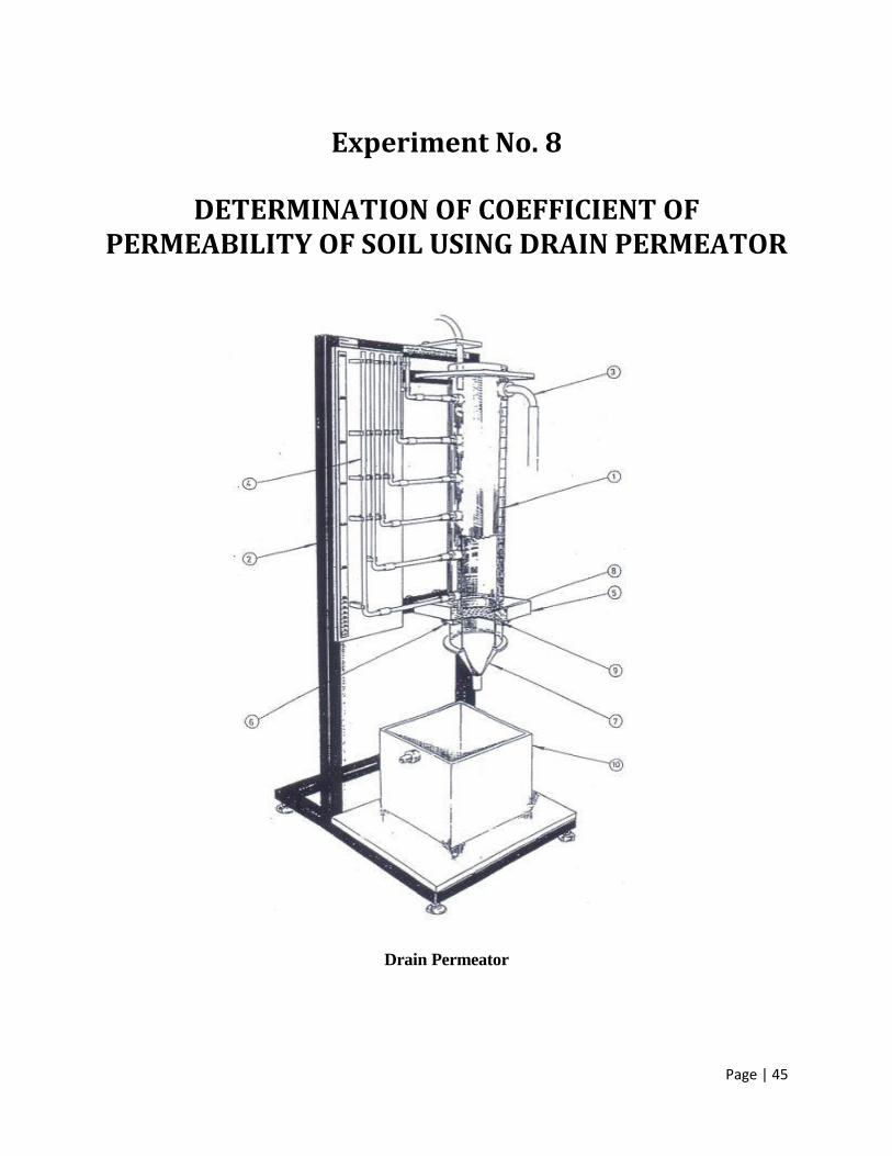
Drain Permeator
Page | 46
Experiment No. 8
DETERMINATION OF COEFFICIENT OF PERMEABILITY OF SOIL USING DRAIN
PERMEATOR
8.1 General
Coefficient of permeability of soil indicates the drainage rate of that particular soil. This
information is useful in determining the amount the flow through the soil. By knowing the drainage
rate of a particular soil, the amount of water that is drained through that soil type for that crop is
known. And this information gives the idea of the time of irrigation.
8.2 Theory
Darcy showed experimentally that, the rate of water Q flowing through soil of cross- sectional area
A is proportional to the hydraulic gradient, i or
Q/A ∞ i or Q = KiA
The coefficient of permeability K has been called “Darcy’s coefficient of permeability” or
“Coefficient of permeability” or “hydraulic conductivity”. The coefficient is not dimensionless but
has the units of velocity. Permeability is a soil property, which indicates the ease with which water
will flow through the soil. Permeability enters all problems involving flow of water through soils,
such as seepage under dams, the squeezing out of water from a soil by the application of a load
and drainage of dams and backfills.
Permeability depends on a number of factors. The main ones are:
(a) The size of soil grains: Permeability appears to be proportional to the square of an effective
grain size. This proportionality is due to the fact that the pore size, which is the primary
variable, is related to particle size.
(b) The properties of pore fluid: Permeability is dependent on fluid viscosity, which in turn is
sensitive to changes in temperature. The following equation expresses the relationship between
viscosity and permeability.
K20˚c = KT μT/ μ20˚c
in which K20˚c = Permeability at temperature 20˚C
KT = Permeability at temperature T˚C
Page | 47
μT = Viscosity of water at temperature T˚C
μ20˚c = Viscosity of water at temperature 20˚C
(c) The void ratio of soil: The more the void ratio, the more will be the permeability of soil. A
permeability of 10-4 cm/sec is frequently used as the borderline between previous (permeability
> 10-4 cm/sec) and impervious (permeability < 10-4 cm/sec) soils.
(d) The shape and arrangement of pores: Although permeability depends on the shapes and
arrangement of pores, this dependence is difficult to express mathematically.
(e) The degree of saturation: An increase in the degree of saturation of a soil causes an increase in
permeability.
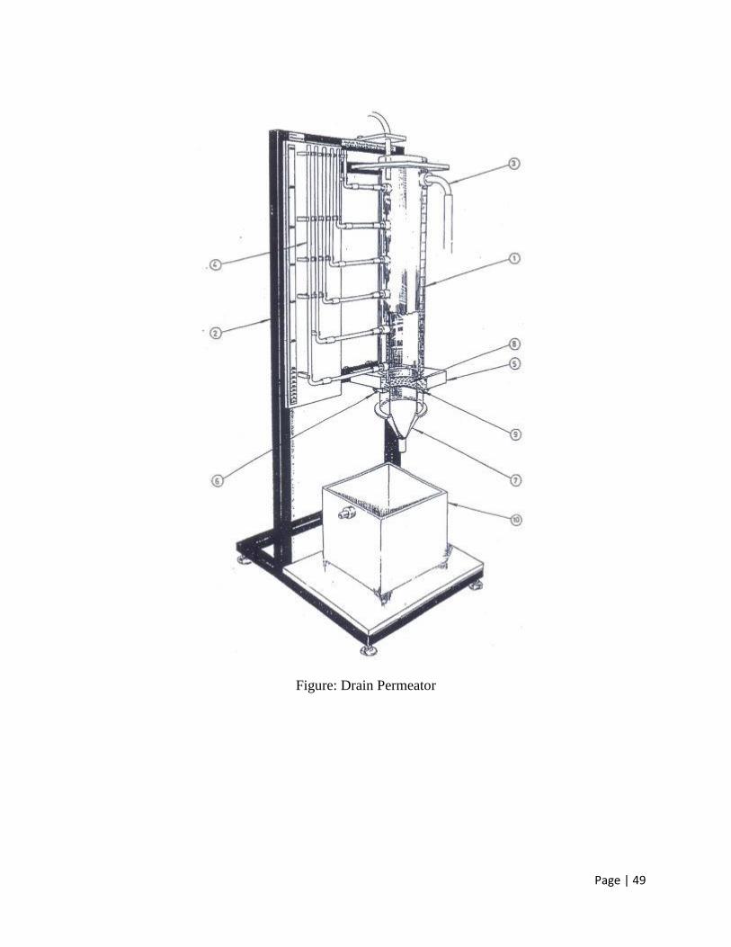
8.3 Description of the Equipment
All numerical references relate to diagram 1. The equipment consists of a vertical perspex cylinder
(1) of 10.8 cm internal diameter and 65 cm long, mounted on a lightweight steel stand (2). The
cylinder has an overflow outlet (3) and six piezometer tappings (4). The bottom support bracket
(5) has four vertical studs (6) protruding from its base, these are used to secure the drain pipe (7),
filters (8) and gaskets (9) to the bracket. The equipment includes two 14 cm by 14 cm gaskets
which are used to prevent lateral leakage from the slotted drains and filters, and two sample drain
materials of different slot shapes and sizes. The drain sample consists of 12 cm diameter discs of
drain pipe. A variety of filter materials are also provided in 13 cm discs. A 20 cm by 20 cm by 20
cm collecting tank (10) with overflow is also provided to collect drainage water. Two lengths of
plastic hose are provided. One for overflow (3) to drain and one to allow water to be admitted from
laboratory supply to top of cylinder.
8.4 Objective
1) To measure the coefficient of permeability of soil.
2) To plot a graph, height of soil coloumn Vs coefficient of permeability of soil.
8.5 Procedure
1) Assemble the apparatus with a slotted drain sample, filter and 10 cm of a sandy soil.
2) Introduce a steady stream of water into the cylinder.
Page | 48
3) Measure the drainage rate by collecting drained water in a measuring beaker over a
measured period of time.
4) When a steady state drainage rate has been achieved. Record the following parameters:
(a) Drainage rate (m3/day) D.
(b) Height of soil column (m) Hs.
(c) Height of water surface above base of soil column (m) Hw.
5) Turn of the water supply.
6) Empty the cylinder of water by using the supply tube as a siphon.
7) Add another 10 cm of soil and repeat steps (i) to (vi) until 4 trials have been run.
8) Record the results in the units indicated on the data sheet.
9) For each trial, calculate the hydraulic conductivity of the soil using the following equation:
K = D × Hs / (πR2 × Hw)
Where,
K = Hydraulic Conductivity (m/d)
R = Radius of the soil column
8.6 Assignments
1) State Darcy’s law. What are the limitations of Darcy’s law?
2) Show mathematically how coefficients of permeability can be calculated for flow –a)
Parallel to the bedding plane and b) Normal to the bedding plane.
3) Show graphically and then explain the relationship between the degree of saturation and
coefficient of permeability.
Page | 49
Figure: Drain Permeator

STUDENT ID: DATE:
Page | 50
Data sheet
DETERMINATION OF COEFFICIENT OF PERMEABILITY OF SOIL USING DRAIN PERMEATOR
Radius of soil column, R =
Trial Drain Rate (m3/day) D Height of Soil (m) Hs Height of Water (m) Hw Area (m2) πR2 Hydraulic
Conductivity (m/d) K
1.
2.
3.
4.
5.
SIGNATURE OF THE TEACHER
---------------------------------------------------
Page | 51
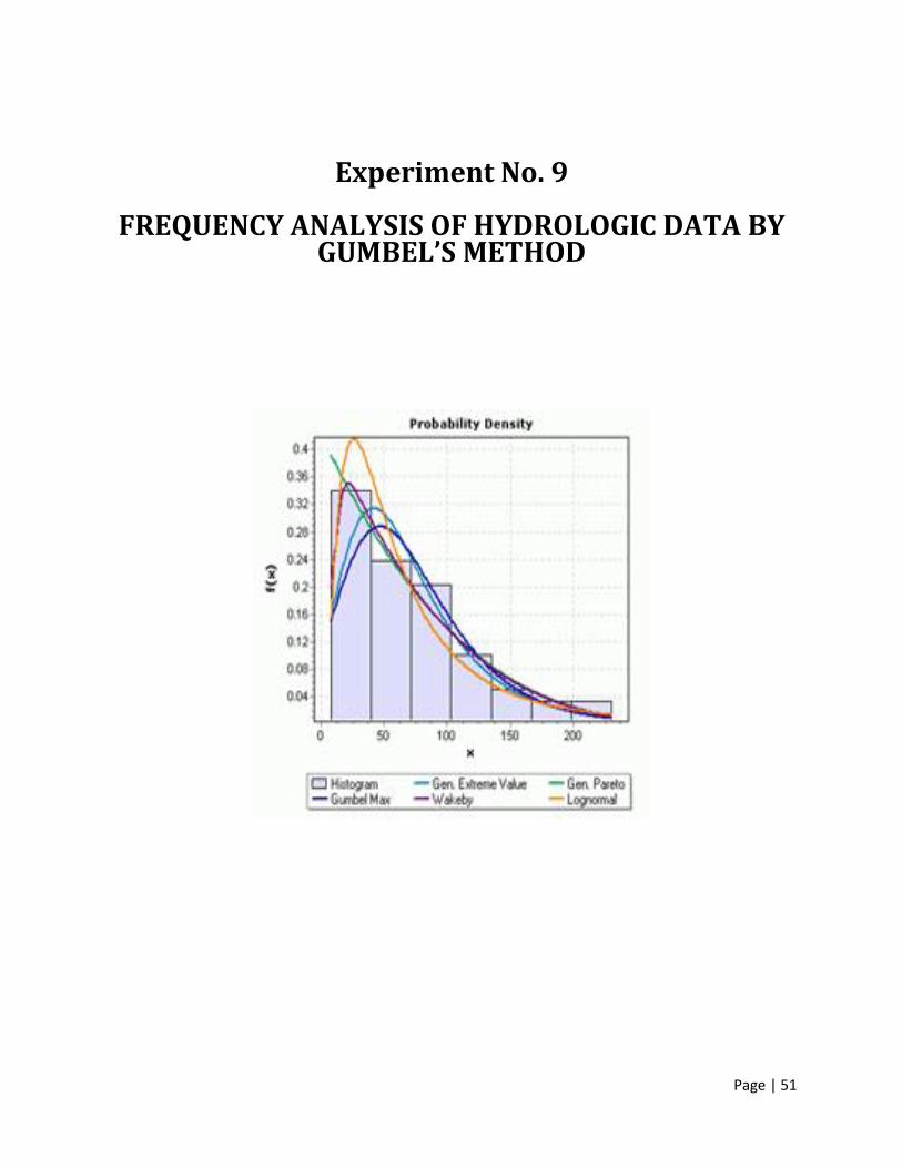
Experiment No. 9
FREQUENCY ANALYSIS OF HYDROLOGIC DATA BY
GUMBEL’S METHOD
Page | 53
Experiment No. 9
FREQUENCY ANALYSIS OF HYDROLOGIC DATA BY GUMBEL’S METHOD
9.1 General
Frequency analysis is very important in the design of practically all hydraulic structures. The peak
flow that can be expected with an assigned frequency is of primary importance to adequately
proportion the hydraulic structure to accommodate its effect. Flood peak values are required in the
design of bridges, culvert, waterways and spillways for dams and also estimation of scour at a
hydraulic structure.
9.2 Theory
9.2.1. Flood Frequency Analysis
Flood frequency analysis is a statistical approach to predict flood flows and estimate the magnitude
of flood peak.
9.2.2. Annual Series
The values of the annual maximum flood from a given catchment area for a large number of
successive years constitute a hydrologic data series called the annual series.
9.2.3. Mean Annual Flood
The value of a flood with a return period T = 2.33 years is called the mean annual flood. When the
sample size is very large Gumble distribution has this property.
9.2.4. Gumble’s Method
The “Extreme value distribution method” was introduced by Gumbel in 1941 and is commonly
known as Gumble’s distribution. It is one of the most widely used probability distribution function
for extreme values in hydrologic and meteorological studies for prediction of flood peaks,
maximum rainfall, maximum wind speed, etc.
Gumble’s equation for practical use (when sample size is finite) is given by,
𝑥𝑇 = �̅� + 𝑘 𝜎𝑛−1 (1)
Where,
𝑥𝑇 = value of the variable 𝑥 of a hydrologic series with a return period T
Page | 54
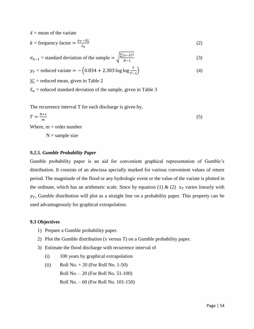
�̅� = mean of the variate
𝑘 = frequency factor =𝑦𝑇 −𝑦𝑛̅̅ ̅̅
𝑆𝑛 (2)
𝜎𝑛−1 = standard deviation of the sample = √∑(𝑥−�̅�)2
𝑁−1 (3)
𝑦𝑇 = reduced variate = − (0.834 + 2.303 log log𝑇
𝑇−1) (4)
𝑦𝑛̅̅ ̅ = reduced mean, given in Table 2
𝑆𝑛 = reduced standard deviation of the sample, given in Table 3
The recurrence interval T for each discharge is given by,
𝑇 =𝑁+1
𝑚 (5)
Where, m = order number
N = sample size
9.2.5. Gumble Probability Paper
Gumble probability paper is an aid for convenient graphical representation of Gumble’s
distribution. It consists of an abscissa specially marked for various convenient values of return
period. The magnitude of the flood or any hydrologic event or the value of the variate is plotted in
the ordinate, which has an arithmetic scale. Since by equation (1) & (2) 𝑥𝑇 varies linearly with
𝑦𝑇, Gumble distribution will plot as a straight line on a probability paper. This property can be
used advantageously for graphical extrapolation.
9.3 Objectives
1) Prepare a Gumble probability paper.
2) Plot the Gumble distribution (x versus T) on a Gumble probability paper.
3) Estimate the flood discharge with recurrence interval of
(i) 100 years by graphical extrapolation
(ii) Roll No. + 20 (For Roll No. 1-50)
Roll No. – 20 (For Roll No. 51-100)
Roll No. – 60 (For Roll No. 101-150)
Page | 55
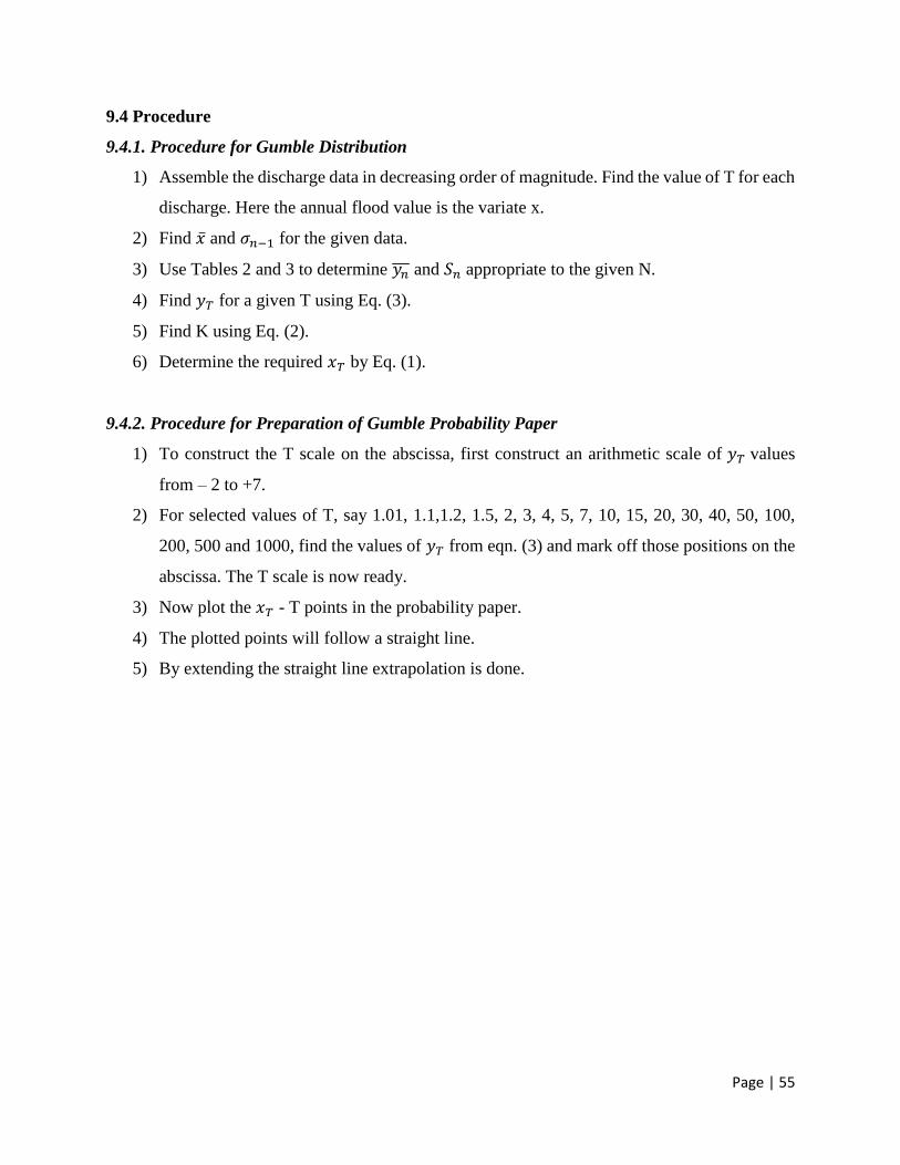
9.4 Procedure
9.4.1. Procedure for Gumble Distribution
1) Assemble the discharge data in decreasing order of magnitude. Find the value of T for each
discharge. Here the annual flood value is the variate x.
2) Find �̅� and 𝜎𝑛−1 for the given data.
3) Use Tables 2 and 3 to determine 𝑦𝑛̅̅ ̅ and 𝑆𝑛 appropriate to the given N.
4) Find 𝑦𝑇 for a given T using Eq. (3).
5) Find K using Eq. (2).
6) Determine the required 𝑥𝑇 by Eq. (1).
9.4.2. Procedure for Preparation of Gumble Probability Paper
1) To construct the T scale on the abscissa, first construct an arithmetic scale of 𝑦𝑇 values
from – 2 to +7.
2) For selected values of T, say 1.01, 1.1,1.2, 1.5, 2, 3, 4, 5, 7, 10, 15, 20, 30, 40, 50, 100,
200, 500 and 1000, find the values of 𝑦𝑇 from eqn. (3) and mark off those positions on the
abscissa. The T scale is now ready.
3) Now plot the 𝑥𝑇 - T points in the probability paper.
4) The plotted points will follow a straight line.
5) By extending the straight line extrapolation is done.
Page | 56
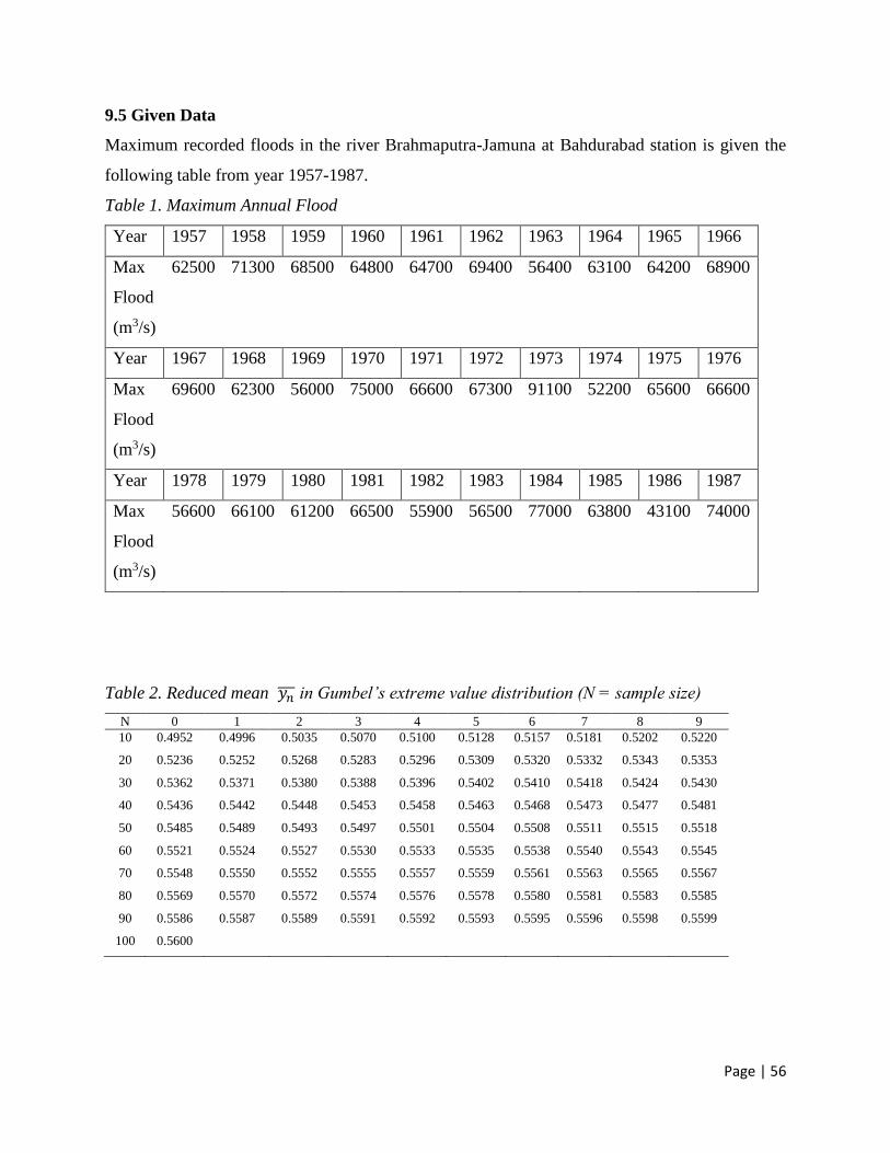
9.5 Given Data
Maximum recorded floods in the river Brahmaputra-Jamuna at Bahdurabad station is given the
following table from year 1957-1987.
Table 1. Maximum Annual Flood
Year 1957 1958 1959 1960 1961 1962 1963 1964 1965 1966
Max
Flood
(m3/s)
62500 71300 68500 64800 64700 69400 56400 63100 64200 68900
Year 1967 1968 1969 1970 1971 1972 1973 1974 1975 1976
Max
Flood
(m3/s)
69600 62300 56000 75000 66600 67300 91100 52200 65600 66600
Year 1978 1979 1980 1981 1982 1983 1984 1985 1986 1987
Max
Flood
(m3/s)
56600 66100 61200 66500 55900 56500 77000 63800 43100 74000
Table 2. Reduced mean 𝑦𝑛̅̅ ̅ in Gumbel’s extreme value distribution (N = sample size)
N 0 1 2 3 4 5 6 7 8 9
10 0.4952 0.4996 0.5035 0.5070 0.5100 0.5128 0.5157 0.5181 0.5202 0.5220
20 0.5236 0.5252 0.5268 0.5283 0.5296 0.5309 0.5320 0.5332 0.5343 0.5353
30 0.5362 0.5371 0.5380 0.5388 0.5396 0.5402 0.5410 0.5418 0.5424 0.5430
40 0.5436 0.5442 0.5448 0.5453 0.5458 0.5463 0.5468 0.5473 0.5477 0.5481
50 0.5485 0.5489 0.5493 0.5497 0.5501 0.5504 0.5508 0.5511 0.5515 0.5518
60 0.5521 0.5524 0.5527 0.5530 0.5533 0.5535 0.5538 0.5540 0.5543 0.5545
70 0.5548 0.5550 0.5552 0.5555 0.5557 0.5559 0.5561 0.5563 0.5565 0.5567
80 0.5569 0.5570 0.5572 0.5574 0.5576 0.5578 0.5580 0.5581 0.5583 0.5585
90 0.5586 0.5587 0.5589 0.5591 0.5592 0.5593 0.5595 0.5596 0.5598 0.5599
100 0.5600
Page | 57
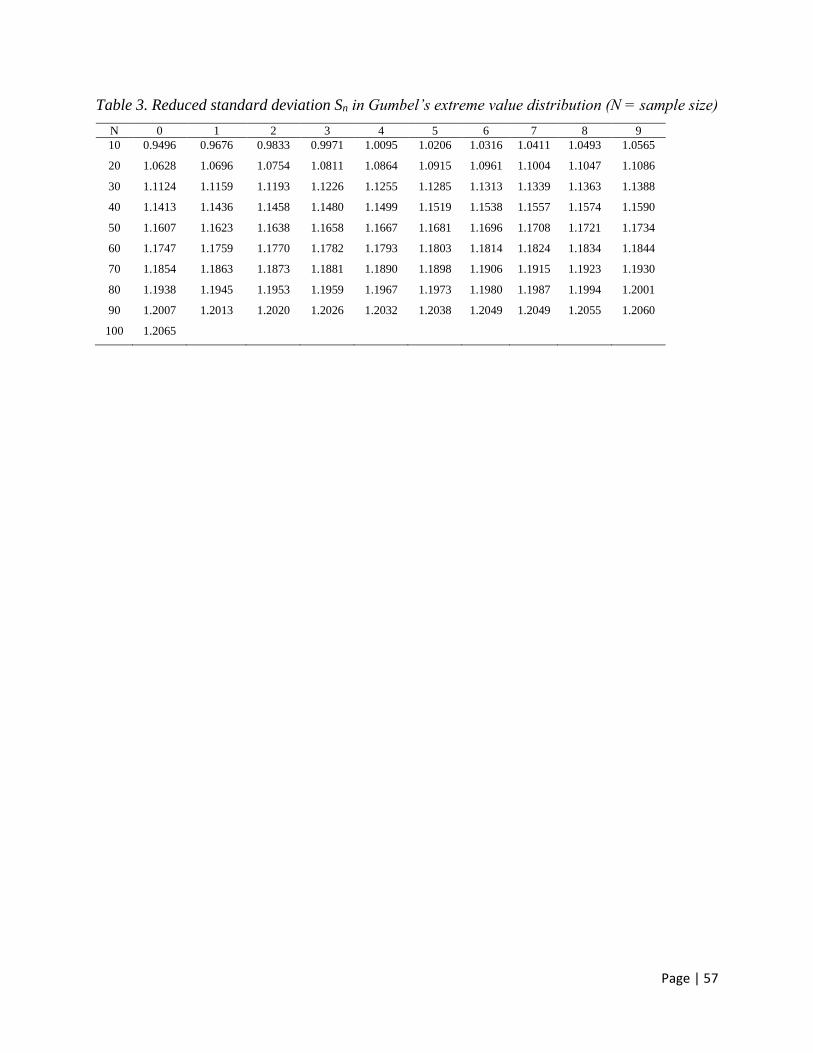
Table 3. Reduced standard deviation Sn in Gumbel’s extreme value distribution (N = sample size)
N 0 1 2 3 4 5 6 7 8 9
10 0.9496 0.9676 0.9833 0.9971 1.0095 1.0206 1.0316 1.0411 1.0493 1.0565
20 1.0628 1.0696 1.0754 1.0811 1.0864 1.0915 1.0961 1.1004 1.1047 1.1086
30 1.1124 1.1159 1.1193 1.1226 1.1255 1.1285 1.1313 1.1339 1.1363 1.1388
40 1.1413 1.1436 1.1458 1.1480 1.1499 1.1519 1.1538 1.1557 1.1574 1.1590
50 1.1607 1.1623 1.1638 1.1658 1.1667 1.1681 1.1696 1.1708 1.1721 1.1734
60 1.1747 1.1759 1.1770 1.1782 1.1793 1.1803 1.1814 1.1824 1.1834 1.1844
70 1.1854 1.1863 1.1873 1.1881 1.1890 1.1898 1.1906 1.1915 1.1923 1.1930
80 1.1938 1.1945 1.1953 1.1959 1.1967 1.1973 1.1980 1.1987 1.1994 1.2001
90 1.2007 1.2013 1.2020 1.2026 1.2032 1.2038 1.2049 1.2049 1.2055 1.2060
100 1.2065

STUDENT ID: DATE:
Page | 58
Data Sheet
FREQUENCY ANALYSIS OF HYDROLOGIC DATA BY GUMBEL’S METHOD
N =
�̅� =
𝜎𝑛−1 =
Flood Discharge, X
(m3/s)
Order number, m 𝑇 = 𝑁+1
𝑚 (years) Flood Discharge, X
(m3/s)
Order number, m 𝑇 = 𝑁+1
𝑚 (years)
SIGNATURE OF THE TEACHER
-------------------------------------------------

STUDENT ID: DATE:
Page | 59
Preparation of Gumbel Probability Paper
RETURN PERIOD, T (Years) 𝑦𝑇
SIGNATURE OF THE TEACHER
-------------------------------------------
Page | 60
Experiment No. 10
HYDROGRAPH ANALYSIS
Page | 61
Experiment No. 10
HYDROGRAPH ANALYSIS
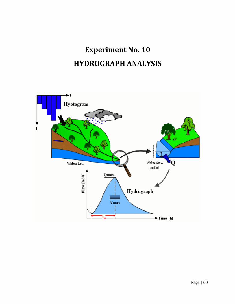
10.1 General
Hydrograph analysis is used for flood routing, flood forecasting and determining design
discharge for any hydraulic structure.
10.2 Theory
Rain falling on a catchment area will make its way to the point of concentration where it will
leave the catchment. In a gravity flow situation, this will be the lowest point in the catchment
if the discharge is through surface stream. On the other hand, if the catchment discharge is
solely by means of ground water movement, the situation is more complex and the flow can
be distributed over a wide front. But in the laboratory the flow is constrained to leave the model
catchment at a single point, we shall not consider this case here.
In practice, a catchment area is defined only once when the point of concentration has been
fixed and as streamflow data are needed here, the site of a new or pre-existing flow
measurement structure is usually chosen. When rain falls on the catchment the time taken for
the water to reach the point of concentration will depend on the horizontal distance it has to
travel and also on the velocity.
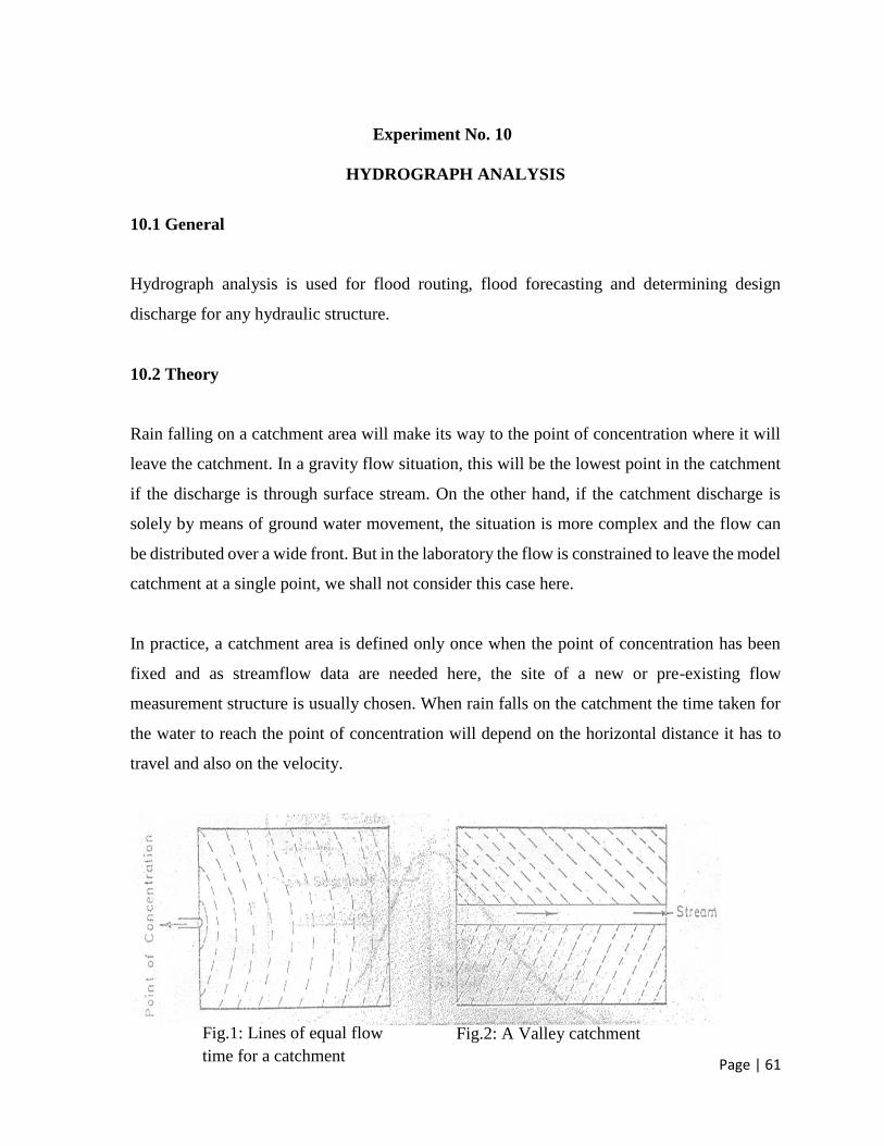
Fig.1: Lines of equal flow
time for a catchment
Fig.2: A Valley catchment
Page | 62
Fig. 1 shows lines of equal flow time for a catchment of similar proportions to the model in
which the flow velocity is everywhere the same. Fig.2 illustrates a valley catchment in which
the flow velocity is assumed to increase once the water has entered the stream channel. Flow
outside the stream could be either surface or ground water flow or both.
10.2.1. Time of concentration:
The time required for water to travel from the most remote portion of the basin to the outlet is
called the time of concentration.
10.2.2. Hydrograph:
A graphical representation of discharge in a stream plotted against time chronologically is
called a hydrograph. Depending upon the units of time involved, hydrographs are,
i. Annual Hydrograph
ii. Monthly Hydrograph
iii. Seasonal Hydrograph
iv. Flood Hydrograph
i. Annual Hydrograph:
Showing variation of daily or weekly or 10 daily mean flows over a year.
ii. Monthly Hydrograph
Showing variation of daily mean flow over a month.
iii. Seasonal Hydrograph
Showing variations of the discharge in a particular season such as the monsoon season or dry
season.
iv. Flood Hydrograph
Hydrographs due to a storm representing stream flow over a catchments.
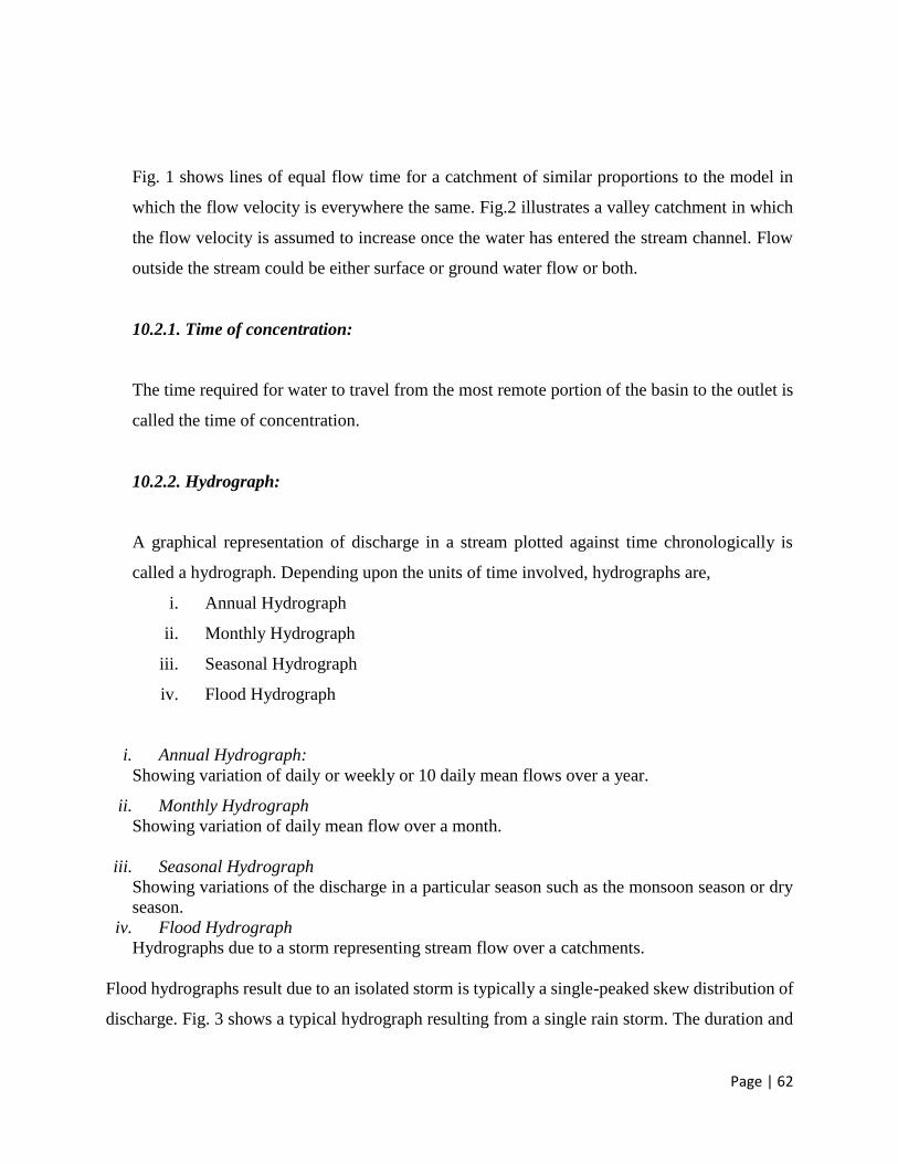
Flood hydrographs result due to an isolated storm is typically a single-peaked skew distribution of
discharge. Fig. 3 shows a typical hydrograph resulting from a single rain storm. The duration and
Page | 63
intensity of the rainfall is shown by the block in the upper part of this figure and if the rainfall
persists for longer than the time of concentration of the catchment, the run-off hydrograph will
level off at the peak value on the catchment. Under these circumstances, the recession curve part
of the hydrograph is delayed until the rain stops.
Fig.3: A typical hydrograph resulting from a single rain storm
During the early stages of the storm, so long as no recent rain has fallen, the ground will be able
to absorb the water falling on it and add it to the ground water already present. When all the voids
are filled, the excess must flow over the surface and enter the stream directly as surface flow. When
the surface flow first reaches the point of concentration it produces a sharp rise in the hydrograph
and this hydrograph discontinuity can be used to separate the ground water contribution from the
direct run-off, as indicated in the figure. The hydrograph shown in Fig.3 is typical for storms of
duration shorter than the time of concentration of the catchment.
The streamflow which is measured during a flood is the result of several watershed functions.
Obviously, a major part of the flood is the result of direct run-off. Surface run-off is the streamflow
which results when the overland flow arrives at a channel. The overland flow regime appears to
Qp
Page | 64
follow a laminar or a distributed laminar type of resistance law. In contrast, the channel flow is
always turbulent.
It is convenient to define the following three parts of a flood hydrograph:
1. Concentration curve or rising limb
2. Crest segment
3. Recession curve or depletion curve or falling limb
The concentration curve exists between the point of rise at the beginning of the flood and the peak
(if it can be recognized) or the point of inflection of the curve on the rising limb just prior to the
peak. The crest segment exists between the point of inflection on the rising side and the point of
inflection on the recession side of the peak. The shape of the rising limb is influenced mainly by
the character of the storm which caused the rise. The point of inflection on the falling side of the
hydrograph is commonly assumed to mark the time at which surface inflow to the channel system
ceases.
10.2.3. Recession Limb:
The recession limb extends from the point of inflection at the end of the crest segment to the
commencement of natural ground water flow. It represents the withdrawal of water from storage
within the basin. The starting point of the recession limb shows the maximum storage. The shape
of the recession is largely independent of the characteristics of the storm causing the rise. However,
the recession curve for a basin is a useful tool in hydrology.
Barnes showed that the following equation could be used to define the recession curve.
𝑄𝑡 = 𝑄𝑜𝐾𝑟𝑒𝑐𝑡 = 𝑄𝑜𝑒−𝛼𝑡 (1)
Where,
𝑄𝑡 = flow t time units after 𝑄𝑜
𝑄𝑜 = flow measured t time earlier
𝐾𝑟𝑒𝑐 = recession constant
t = time in between 𝑄𝑜&𝑄𝑡
e = napierian base
α = − ln 𝐾𝑟𝑒𝑐
Eq. (1) will plot as a straight line on semi-logarithmic graph paper provided 𝐾𝑟𝑒𝑐 for groundwater
(𝐾𝑟𝑏) since, presumably, both interflow and surface runoff have ceased. By projecting this slope
Page | 65
backyard in time and replotting the difference between the projected line and the total hydrograph,
a recession which for a time consists largely of interflow is obtained. With the slope applicable to
interflow thus detrmined, the process can be repeated to establish the recession characteristics of
surface runoff.
10.2.4. Base flow separation:
Base flow may be separated by any of the following three methods.
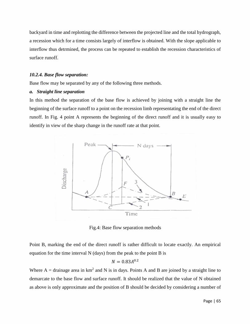
a. Straight line separation
In this method the separation of the base flow is achieved by joining with a straight line the
beginning of the surface runoff to a point on the recession limb representating the end of the direct
runoff. In Fig. 4 point A represents the beginning of the direct runoff and it is usually easy to
identify in view of the sharp change in the runoff rate at that point.
Fig.4: Base flow separation methods
Point B, marking the end of the direct runoff is rather difficult to locate exactly. An empirical
equation for the time interval N (days) from the peak to the point B is
𝑁 = 0.83𝐴0.2
Where A = drainage area in km2 and N is in days. Points A and B are joined by a straight line to
demarcate to the base flow and surface runoff. It should be realized that the value of N obtained
as above is only approximate and the position of B should be decided by considering a number of
Page | 66
hydrographs for the catchment. This method of base flow separation is the simplest of all three
methods.
b. Fixed base length separation
In this method the base flow curve existing prior to the commencement of the surface runoff is
extended till it intersects the ordinate drawn at the peak (point C in Fig. 4). This point joined to
point B by a straight line. Segment AC and CB demarcate the base flow and surface runoff. This
is probably the most widely used base flow separation procedure.
c. Variable slope separation
In this method the base flow recession curve after the depletion of the flood water is extended
backwards till it intersects the ordinate at the point of inflection (line EF in Fig. 4). Points A and
F are joined by an arbitrary smooth curve. This method of base-flow separation is realistic in
situations where the groundwater contributions are significant and reach the stream quickly.
It is seen that all the three methods of base-flow separation are rather arbitrary. The selection of
any one of them depends upon the local practice and successful predictions achieved in the past.
The surface runoff hydrograph obtained after the base-flow separation is also known as direct
runoff hydrograph (DRH).
10.2.5. Unit Hydrograph
A unit hydrograph is defined as the hydrograph of direct runoff resulting from one unit depth (1
cm) of rainfall excess occurring uniformly over the catchment and at a uniform rate for a specified
duration (D-h). This will be known as D-h unit hydrograph. If an appropriate unit hydrograph is
available, one can easily calculate the Direct Runoff Hydrograph (DRH) in a catchment due to a
given storm.
10.2.6. S-curve
The S-curve, also known as S-hydrograph, is a hydrograph produced by a continuous effective
rainfall at a constant rate for an infinite period. It is a curve obtained by summation of an infinite
series of D-h unit hydrographs spaced D-h apart. S-curve is used to develop a unit hydrograph of
duration mD, where m is a fraction.
Page | 67
10.2.7. Instantaneous Unit Hydrograph
The limiting case of a unit hydrograph of zero duration is known as instantaneous unit hydrograph
(IUH). Thus IUH is a fictitious, conceptual unit hydrograph which represents the surface runoff
from the catchment due to an instantaneous precipitation of the rainfall excess of 1 cm. For a given
catchment IUH, being independent of the rainfall characteristics, is indicative of the basin storage
characteristics.
10.2.8. Synthetic Unit Hydrograph
Unit hydrographs can be derived only if records of rainfall and the resulting flood hydrograph are
available. Since only a relatively small portion of catchments are gaged, some means of deriving
unit hydrographs for ungaged catchments is necessary. In order to construct unit hydrographs for
such areas, empirical equations of regional validity which relate the salient hydrograph
characteristics to the basin characteristics are needed. Unit hydrographs derived from such
relationships are known as synthetic unit hydrographs.
10.3 Procedure
1) This experiment is done in the basic hydrologic system.
2) There is a artificial sand bed in the setup.
3) First artificial rainfall is created.
4) Reading of runoff starts at the beginning of rainfall.
5) Reading is recorded at every 10 second interval.
6) The rainfall will be stopped after 100 sec.
7) Reading is continued up to two consecutive readings become same.
8) The total hydrograph is then plotted in a plain graph paper.
9) The recession limb will be plotted on semi log paper.
10) A tangent is drawn at the constant value of the recession limb.
11) The slope of this tangent gives the recession constant for base flow (𝐾𝑟𝑏).
12) The ordinates of the tangent give the value of the base flow.
13) Now by subtracting the ordinates of this tangent from the total runoff we get the hydrograph
for interflow and surface runoff.
14) If interflow is neglected i.e. taking the recession constant for interflow 1, then the surface
runoff is calculated by subtracting the ordinate of base flow from the total hydrograph.

Page | 68
Surface runoff = Total runoff – base flow
10.4 Objective
1) To draw the recession limb of hydrograph on a semi-log paper.
2) To find the recession constant for base flow.
3) To find the recession constant for interflow.
4) To find the recession constant for surface run-off.
5) To find the surface run-off.
10.5 Assignment
1) What is surface run-off?
2) What is the time of concentration?
3) What is a synthetic unit hydrograph?
4) What is an S-curve?
5) Distinguish between lag time and time to peak.
6) Draw a neat figure of a hydrologic cycle and show the following in it:
a. Surface run-off
b. Ground water flow
c. Evaporation
d. Transpiration

STUDENT ID: DATE:
Page | 69
Data Sheet
HYDROGRAPH ANALYSIS
Area of watershed =
Duration of rainfall =
Time Discharge Time Discharge Time Discharge
SIGNATURE OF THE TEACHER
-------------------------------------------------

STUDENT ID: DATE:
Page | 70
Computation of Recession Constants
SIGNATURE OF THE TEACHER
Time Recorded
hydrograph,
Total runoff
Recession
constant for
base flow
𝐾𝑟𝑏
Base flow Surface
runoff
Recession
constant for
surface
runoff 𝐾𝑟𝑠
REFERENCES
1. Garg, S.K., Irrigation Engineering and Hydraulic Structures, Khanna Publishers, Delhi-
21st Edition (April, 2007).
2. Daugherty, R.L., Franzini, J.B. and Finnemore, E.J., Fluid Mechanics with Engineering
Applications, McGraw-Hill Book Co, Singapore-1989.
3. Department of Water Resources Engineering, Bangladesh University of Engineering
and Technology, Irrigation and Drainage Sessional (August-2015).
Appendix Lab Report Format
1. All students must have a same colored printed cover page. The design of cover page is
provided with the lab manual. Students have to compose only the course teacher’s name
and designation and their information.
2. An index is provided. It should be printed and set after the cover page. Table may be
filled up by pen during each submission after test.
3. Each report must have a common printed top page. Only the experiment name and no.
and the date may be filled up by pen. A top page design is provided.
4. A4 papers have to be used for preparing the lab report. Writing should be done with
pen. Pencil may be used for any kind of sketch.
5. In each experiment of the lab report the following points must have to be present:
Objective, Equipment, Procedure, Data Table (signed), Sample Calculation,
Result, Discussion and Assignment.
CE 472 Water Resources Engineering Sessional-II
(Lab Report)
Prepared For
Name of Course Teacher
Designation of Course Teacher
&
Name of Course Teacher
Designation of Course Teacher
Prepared By
Name of Student
Student’s ID
Year/ Semester
Group

INDEX
Experiment
no.
Experiment Name Date of
Performance
Date of
Submission
Signature Comments Page
no.

INDEX
Experiment
no.
Experiment Name Date of
Performance
Date of
Submission
Signature Comments Page
no.
CE 472 Water Resources Engineering Sessional-II
(Lab Report)
Experiment No. :
Experiment Name:
Date of Performance:
Date of Submission:
Prepared For
Name of Course Teacher
Designation of Course Teacher
&
Name of Course Teacher
Designation of Course Teacher
Prepared By
Name of Student
Student’s ID
Year/ Semester
Group

Appendix 3
Lab Instructions
1. All students must have to be present at the class just in time.
2. All students must have to submit the lab report just after the entrance and before the
class start.
3. Lab reports have to be submitted serially according to Student’s ID.
4. Students have to complete the data sheet in class and complete sample calculations and
graphs in class and take sign from the course teacher. (In some experiment which
require more times, data sheet should be completed as possible in class time.)
Recommended