1
CHAPTER 3 -- PROBLEMS AND EXERCISES
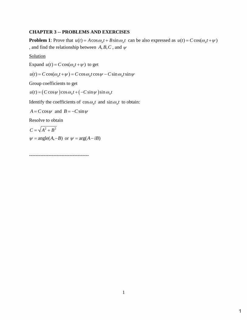
Problem 1: Prove that ( ) cos sinn nu t A t B t can be also expressed as ( ) cos( )nu t C t , and find the relationship between , ,A B C , and
Solution
Expand ( ) cos( )nu t C t to get
( ) cos( ) cos cos sin sinn n nu t C t C t C t
Group coefficients to get
( ) cos cos sin sinn nu t C t C t
Identify the coefficients of cos nt and sin nt to obtain:
cosA C and sinB C
Resolve to obtain
2 2C A B
angle( , )A B or arg( )A iB
-------------------------------------
1

angle A B( ) 126.87 deg
A i B 5arg A i B( ) 126.87 degB 4A 3
angle A B( ) 233.13 deg
A i B 5arg A i B( ) 126.87 degB 4A 3
angle A B( ) 53.13 deg
A i B 5arg A i B( ) 53.13 degB 4A 3
angle A B( ) 306.87 deg
A i B 5arg A i B( ) 53.13 degB 4A 3
Here are some examples of using the absolute value and angle or arg functions:
PROBLEM 3.1 SOLUTION
2
2
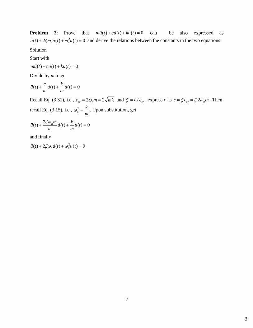
Problem 2: Prove that ( ) ( ) ( ) 0mu t cu t ku t can be also expressed as 2( ) 2 ( ) ( ) 0n nu t u t u t and derive the relations between the constants in the two equations
Solution
Start with
( ) ( ) ( ) 0mu t cu t ku t
Divide by m to get
( ) ( ) ( ) 0c k
u t u t u tm m
Recall Eq. (3.31), i.e., 2 2cr nc m mk and / crc c . express c as 2cr nc c m . Then,
recall Eq. (3.15), i.e., 2n
k
m . Upon substitution, get
2( ) ( ) ( ) 0nm k
u t u t u tm m
and finally,
2( ) 2 ( ) ( ) 0n nu t u t u t
3
3
Problem 3: Prove that 1 2( ) n d n di t i tu t C e C e can be rewritten as
( ) cos( )ntdu t Ce t and derive the relations between the constants in the two equations
Solution
Expand and group 1 2( ) n d n di t i tu t C e C e to get
1 2 1 2( ) n d n d n d di t i t t i t i tu t C e C e e C e C e
Use Euler identity cos sinie i to write
1 2 1 2
1 2 1 2
(cos sin ) (cos sin )
cos sin
d di t i td d d d
d d
C e C e C t t C t t
C C t C C t
Now, consider ( ) cos( )ntdu t Ce t and expand it to get
( ) cos( ) cos cos sin sin
cos cos sin sin
n n
n
t td d d
td d
u t Ce t Ce t t
e C t C t
Identifying coefficients between the two expressions, we establish
1 2
1 2
cos
sin
C C C
C C C
Upon solution,
11 2
12 2
cos sin
cos sin
C C
C C
Conversely,
2 21 2 1 2C C C C C
1 2 1 2angle ,C C C C or 1 2 1 2arg C C i C C
-------------------------------------
4

4
Problem 4: Prove that when damping equals critical damping ( 1 ), the solution of 2( ) 2 ( ) ( ) 0n nu t u t u t is 1 2( ) ntu t C C t e
Solution
Recall Eq. (3.30), 2( ) 2 ( ) ( ) 0n nu t u t u t , and the characteristic equation (3.32), 2 22 0n n . If 1 , then these two equations become
2( ) 2 ( ) ( ) 0n nu t u t u t
2 22 0n n
The characteristic equation has the double root, 1 2 n .
The general ODE theory shows that if the characteristic equation has a double root, say a, then both ate and atte are solutions of the ODE. Indeed, assume the ODE is 2( ) 2 ( ) ( ) 0u t au t a u t , which has the characteristic equation 2 22 0a a with the double root 1 2 a . Let’s
verify that both 1atu e and 2
atu te are solutions. The proof for 1u is easily obtained through
direct substitution and will not be elaborated here. The proof for 2u is obtained by substitution as
follows:
2atu te
2at at atu te e tae
2 22 2at at at at at at atu e tae ae ae ta e ae ta e
The notations and were used to signify first and second derivatives. Upon substitution
into the differential equation, we get
2 22 2
2
at at at at at
at
ae ta e a e tae a te
ae
2 atta e 2 atae 2 atatae 2 ata te 0
Thus we have proved that both 1atu e and 2
atu te are solutions. Hence, the general solution is
a linear combination of these two solutions, i.e.,
1 2( ) atu t C C t e
To finalize the proof of the exercise, simply observer that na . Hence, the general solution is
1 2( ) ntu t C C t e
-------------------------------------
5
5
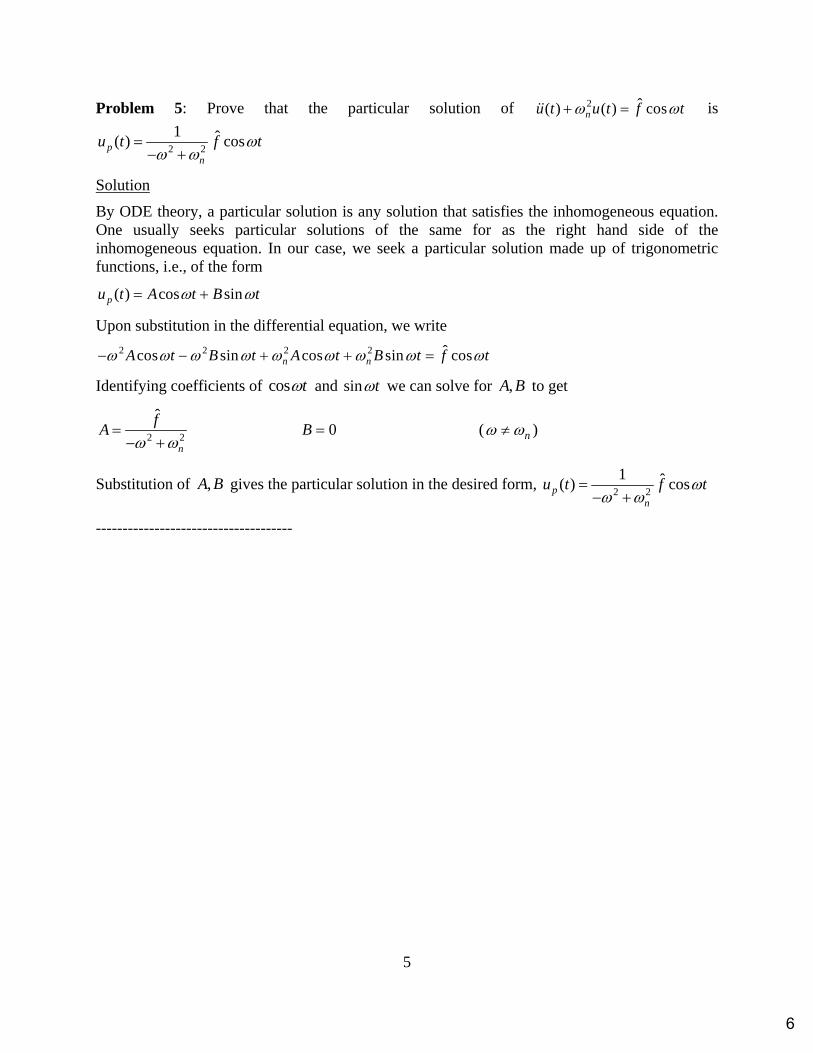
Problem 5: Prove that the particular solution of 2 ˆ( ) ( ) cosnu t u t f t is
2 2
1 ˆ( ) cospn
u t f t
Solution
By ODE theory, a particular solution is any solution that satisfies the inhomogeneous equation. One usually seeks particular solutions of the same for as the right hand side of the inhomogeneous equation. In our case, we seek a particular solution made up of trigonometric functions, i.e., of the form
( ) cos sin pu t A t B t
Upon substitution in the differential equation, we write
2 2 2 2 ˆcos sin cos sin cos n nA t B t A t B t f t
Identifying coefficients of cost and sint we can solve for ,A B to get
2 2
ˆ
n
fA
0B ( n )
Substitution of ,A B gives the particular solution in the desired form, 2 2
1 ˆ( ) cospn
u t f t
-------------------------------------
6
6
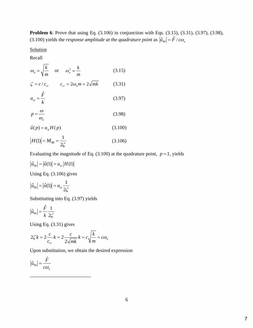
Problem 6: Prove that using Eq. (3.106) in conjunction with Eqs. (3.15), (3.31), (3.97), (3.98), (3.100) yields the response amplitude at the quadrature point as 90
ˆˆ / nu F c
Solution
Recall
nk
m or 2
n
k
m (3.15)
/ crc c 2 2cr nc m mk (3.31)
ˆst
Fu
k (3.97)
n
p
(3.98)
ˆ( ) ( )stu p u H p (3.100)
901
(1)2
H M
(3.106)
Evaluating the magnitude of Eq. (3.100) at the quadrature point, 1p , yields
90ˆ ˆ(1) (1) stu u u H
Using Eq. (3.106) gives
90
1ˆ ˆ(1)
2 stu u u
Substituting into Eq. (3.97) yields
90
ˆ 1ˆ
2
Fu
k
Using Eq. (3.31) gives
2 2 22
ncr
c c kk k k c c
c mmk
Upon substitution, we obtain the desired expression
90
ˆˆ
n
Fu
c
-------------------------------------
7
7
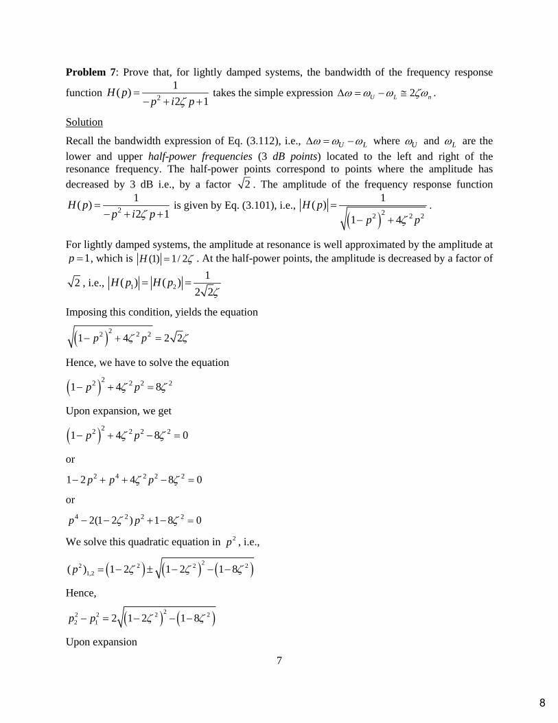
Problem 7: Prove that, for lightly damped systems, the bandwidth of the frequency response
function 2
1( )
2 1H p
p i p
takes the simple expression 2U L n .
Solution
Recall the bandwidth expression of Eq. (3.112), i.e., U L where U and L are the
lower and upper half-power frequencies (3 dB points) located to the left and right of the resonance frequency. The half-power points correspond to points where the amplitude has
decreased by 3 dB i.e., by a factor 2 . The amplitude of the frequency response function
2
1( )
2 1H p
p i p
is given by Eq. (3.101), i.e.,
22 2 2
1( )
1 4H p
p p
.
For lightly damped systems, the amplitude at resonance is well approximated by the amplitude at 1p , which is (1) 1/ 2H . At the half-power points, the amplitude is decreased by a factor of
2 , i.e., 1 2
1( ) ( )
2 2H p H p
Imposing this condition, yields the equation
22 2 21 4 2 2p p
Hence, we have to solve the equation
22 2 2 21 4 8p p
Upon expansion, we get
22 2 2 21 4 8 0p p
or
2 4 2 2 21 2 4 8 0p p p
or
4 2 2 22(1 2 ) 1 8 0p p
We solve this quadratic equation in 2p , i.e.,
22 2 2 21,2( ) 1 2 1 2 1 8p
Hence,
22 2 2 22 1 2 1 2 1 8p p
Upon expansion
8

8
2 22 1 2 1p p 2 44 4 1 2
2 4
8
2 4 4
Using the light damping approximation ( 1 ) we ignore the term in 4 and write
2 2 2 42 1 2 4 4p p 22 4
The left hand side can be expanded into sum and difference product, i.e.,
22 1 2 1 2 4p p p p
For light damping, the 1p and 2p values are approximately balanced about the resonance point
1p , and thus 1 2 2p p . Hence, the above expression becomes
22 1 4 2p p
In terms of physical frequencies, the above expression is written as
2U L n
The proof is complete.
-------------------------------------
9
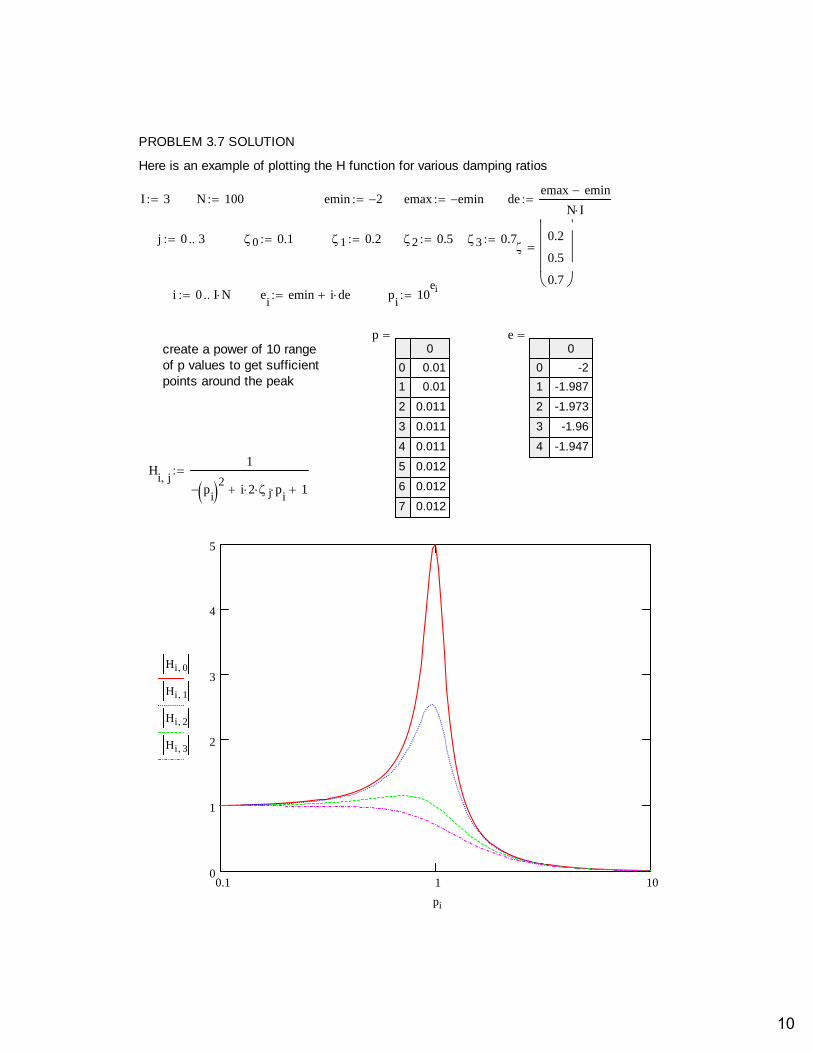
0.1 1 100
1
2
3
4
5
Hi 0
Hi 1
Hi 2
Hi 3
pi
Hi j
1
pi 2 i 2 j p
i 1
create a power of 10 rangeof p values to get sufficient points around the peak
e0
0
1
2
3
4
-2
-1.987
-1.973
-1.96
-1.947
p0
0
1
2
3
4
5
6
7
0.01
0.01
0.011
0.011
0.011
0.012
0.012
0.012
pi
10eie
iemin i dei 0 I N
0.1
0.2
0.5
0.7
3 0.72 0.51 0.20 0.1j 0 3
deemax emin
N Iemax eminemin 2N 100I 3
Here is an example of plotting the H function for various damping ratios
PROBLEM 3.7 SOLUTION
10
9
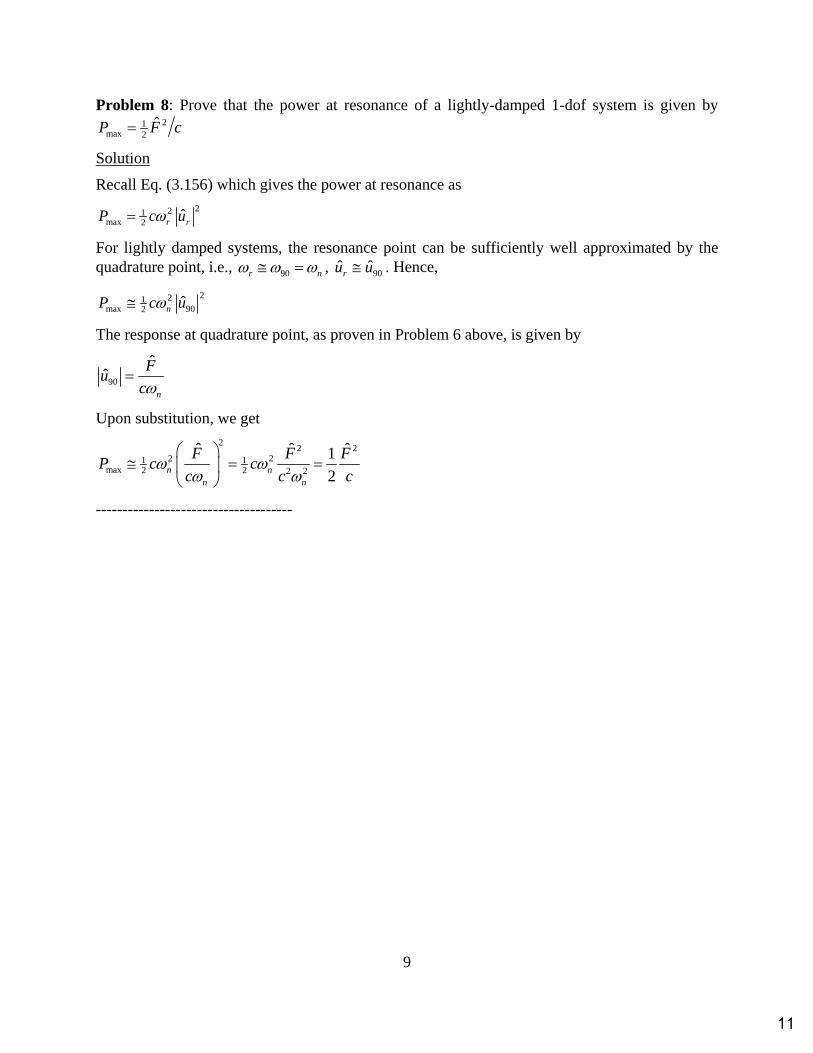
Problem 8: Prove that the power at resonance of a lightly-damped 1-dof system is given by 21
max 2ˆP F c
Solution
Recall Eq. (3.156) which gives the power at resonance as 221
max 2ˆr rP c u
For lightly damped systems, the resonance point can be sufficiently well approximated by the quadrature point, i.e., 90r n , 90ˆ ˆru u . Hence,
221max 902
ˆnP c u
The response at quadrature point, as proven in Problem 6 above, is given by
90
ˆˆ
n
Fu
c
Upon substitution, we get 2
2 22 21 1
max 2 2 2 2
ˆ ˆ ˆ1
2n nn n
F F FP c c
c c c
-------------------------------------
11

10
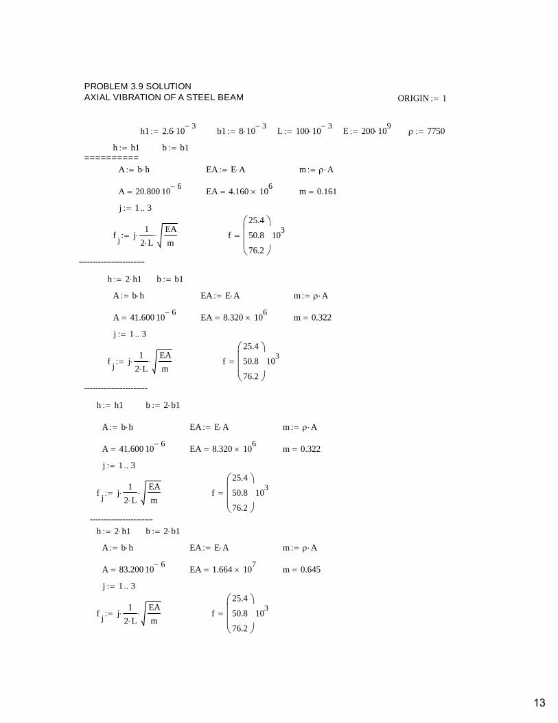
Problem 9: Find the first, second, and third natural frequencies of in-plane axial vibration of a steel beam of thickness h1 = 2.6 mm, width b1 = 8 mm, length l = 100 mm, modulus E = 200 GPa, and density = 7.750 g/cm3. The beam is in free-free boundary conditions. Then, consider double the thickness (h2 = 5.2 mm), wider width (b2 = 19.6 mm), and then both. Recalculate the three frequencies for these other combinations of thickness and width. Discuss your results
Solution
Recall Eq. (3.192), i.e., 1
2j
EAf j
l m , j = 1,2,3.
Use geometric dimensions and material properties to calculate 220.8 mmA ; 4.16 MNEA ; 0.161 kg/mm
Substitute in the frequency equation to get
1 25.4 kHzf ; 2 50.8 kHzf ; 3 76.2 kHzf
Double the thickness 241.6 mmA ; 8.32 MNEA ; 0.322 kg/mm
Substitute in the frequency equation to get
1 25.4 kHzf ; 2 50.8 kHzf ; 3 76.2 kHzf
The frequencies do not change because the changes in EA are compensated by the changes in m.
Double the width 241.6 mmA ; 8.32 MNEA ; 0.322 kg/mm
Substitute in the frequency equation to get
1 25.4 kHzf ; 2 50.8 kHzf ; 3 76.2 kHzf
The frequencies do not change because the changes in EA are compensated by the changes in m.
Double the thickness and the width 283.2 mmA ; 16.64 MNEA ; 0.645 kg/mm
Substitute in the frequency equation to get
1 25.4 kHzf ; 2 50.8 kHzf ; 3 76.2 kHzf
The frequencies do not change because the changes in EA are compensated by the changes in m.
-------------------------------------
12
j 1 3
fj
j1
2 L
EA
m f
25.4
50.8
76.2
103
-----------------------
h h1 b 2 b1
A b h EA E A m A
A 41.600 106
EA 8.320 106
m 0.322
j 1 3
fj
j1
2 L
EA
m f
25.4
50.8
76.2
103
-----------------------h 2 h1 b 2 b1
A b h EA E A m A
A 83.200 106
EA 1.664 107
m 0.645
j 1 3
fj
j1
2 L
EA
m f
25.4
50.8
76.2
103
PROBLEM 3.9 SOLUTIONAXIAL VIBRATION OF A STEEL BEAM ORIGIN 1
h1 2.6 103
b1 8 103
L 100 103
E 200 109
7750
h h1 b b1==========
A b h EA E A m A
A 20.800 106
EA 4.160 106
m 0.161
j 1 3
fj
j1
2 L
EA
m f
25.4
50.8
76.2
103
------------------------
h 2 h1 b b1
A b h EA E A m A
A 41.600 106
EA 8.320 106
m 0.322
13
11
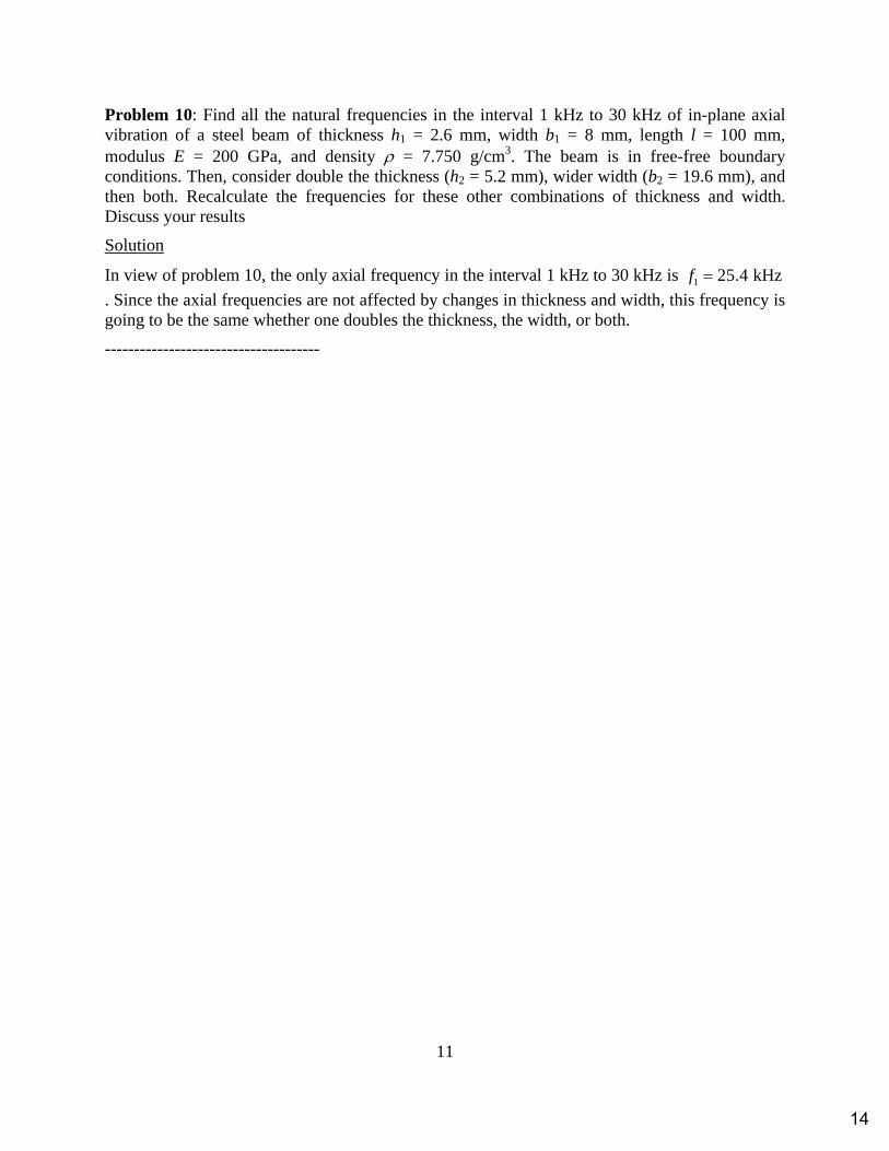
Problem 10: Find all the natural frequencies in the interval 1 kHz to 30 kHz of in-plane axial vibration of a steel beam of thickness h1 = 2.6 mm, width b1 = 8 mm, length l = 100 mm, modulus E = 200 GPa, and density = 7.750 g/cm3. The beam is in free-free boundary conditions. Then, consider double the thickness (h2 = 5.2 mm), wider width (b2 = 19.6 mm), and then both. Recalculate the frequencies for these other combinations of thickness and width. Discuss your results
Solution
In view of problem 10, the only axial frequency in the interval 1 kHz to 30 kHz is 1 25.4 kHzf . Since the axial frequencies are not affected by changes in thickness and width, this frequency is going to be the same whether one doubles the thickness, the width, or both.
-------------------------------------
14

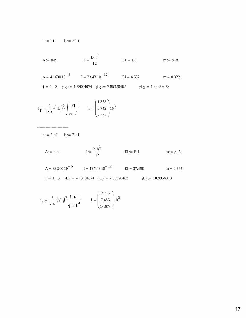
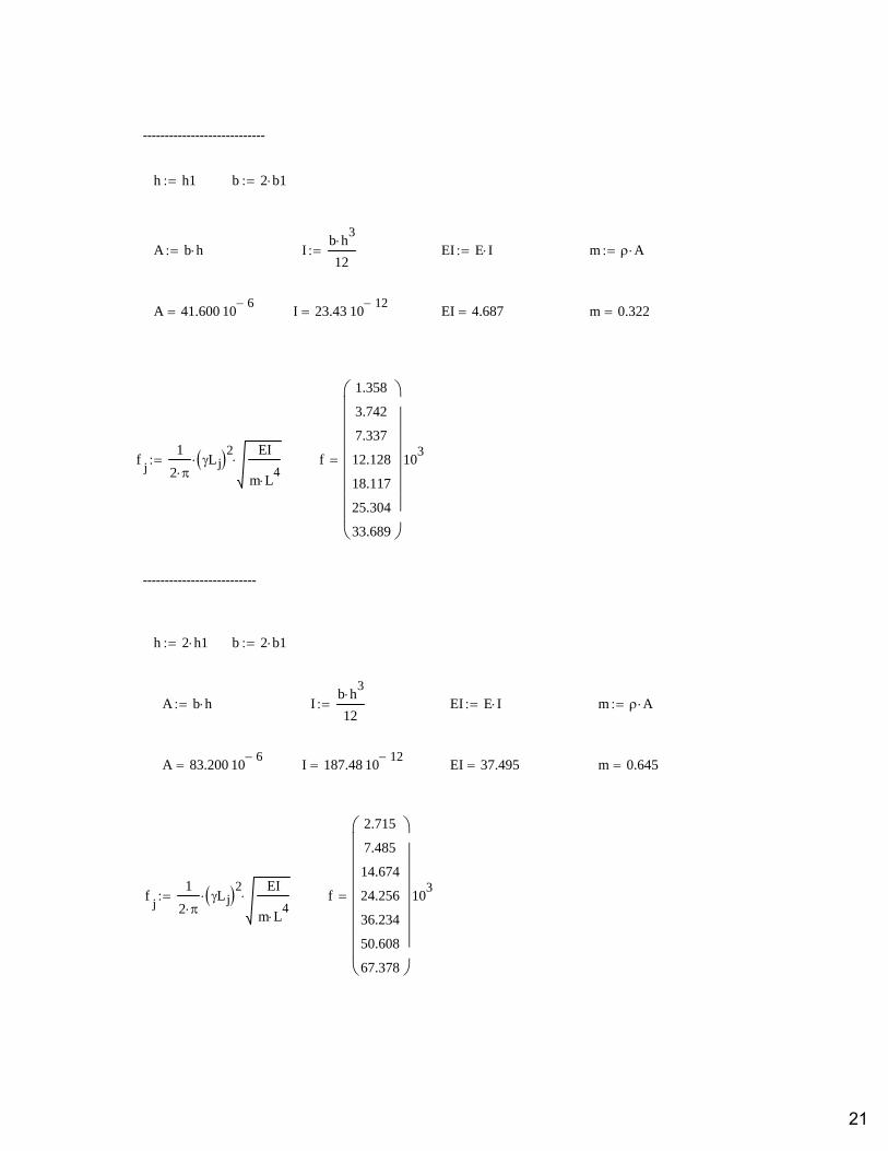
12
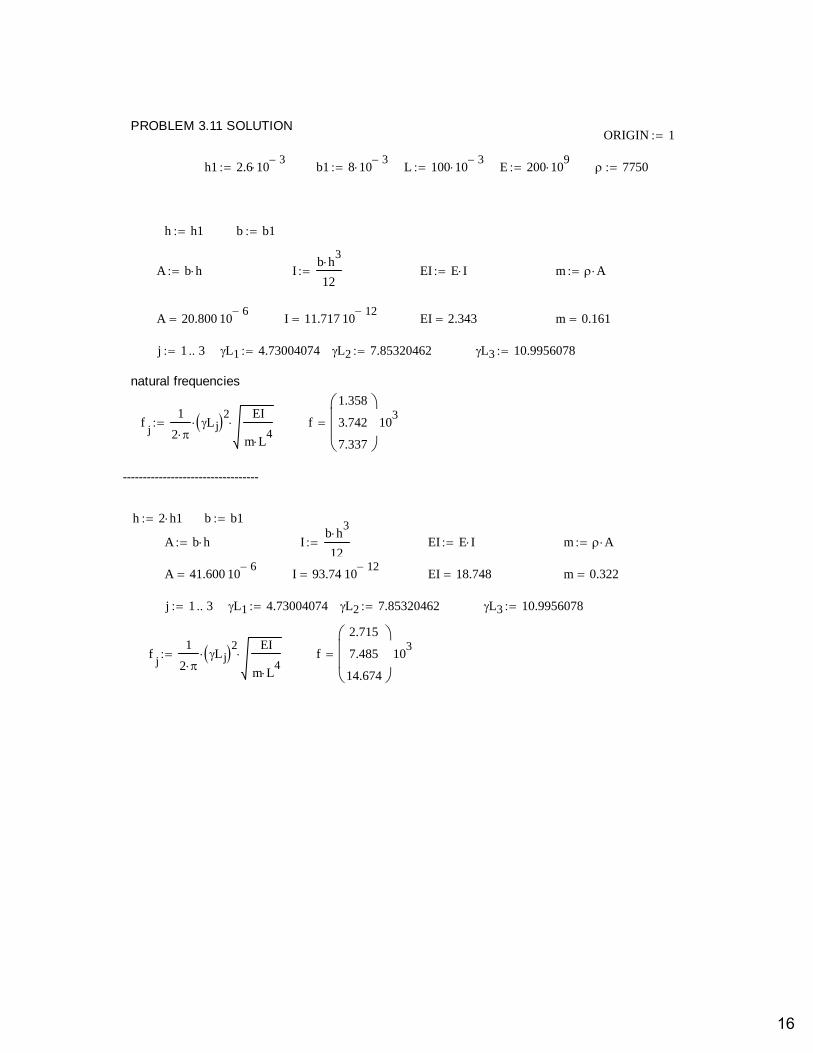
Problem 11: Find the first, second, and third natural frequencies of out-of-plane flexural vibration of a steel beam of thickness h1 = 2.6 mm, width b1 = 8 mm, length l = 100 mm, modulus E = 200 GPa, and density = 7.750 g/cm3. The beam is in free-free boundary conditions. Then, consider double the thickness (h2 = 5.2 mm), wider width (b2 = 19.6 mm), and then both. Recalculate the three frequencies for these other combinations of thickness and width. Discuss your results
Solution
Recall Eq. (3.408), i.e., 24
1
2j j
EIf z
ml j = 1,2,3
Use geometric dimensions and material properties to calculate 220.8 mmA ; 411.717 mmI ; 22.343 NmEI ; 0.161 kg/mm
Get the values of l from Table 3.5. Substitute in the frequency equation to get
1 1.358 kHzf ; 2 3.742 kHzf ; 3 7.337 kHzf
Double the thickness 241.6 mmA ; 493.74 mmI ; 218.748 NmEI ; 0.322 kg/mm
Get the values of l from Table 3.5. Substitute in the frequency equation to get
1 2.715 kHzf ; 2 7.485 kHzf ; 3 14.674 kHzf
The frequencies have increased because EI increases as 3h whereas m increases only as h. The faster increase in EI has produced increase in frequency.
Double the width 241.6 mmA ; 423.43 mmI ; 24.687 NmEI ; 0.322 kg/mm
Get the values of l from Table 3.5. Substitute in the frequency equation to get
1 1.358 kHzf ; 2 3.742 kHzf ; 3 7.337 kHzf
The frequencies have not increased because both EI and m increase as b.
Double the thickness and the width 283.2 mmA ; 4187.48 mmI ; 237.495 NmEI ; 0.645 kg/mm
Get the values of l from Table 3.5. Substitute in the frequency equation to get
1 2.715 kHzf ; 2 7.485 kHzf ; 3 14.674 kHzf
The frequencies have increased in the same amount as for just double the thickness h. This is because EI increases as 3bh whereas m increases as bh , indicating that thickness increase affects the flexural frequencies but width increase does not.
15
natural frequencies
fj
1
2 Lj 2
EI
m L4
f
1.358
3.742
7.337
103
----------------------------------
h 2 h1 b b1
A b h Ib h
3
12 EI E I m A
A 41.600 106
I 93.74 1012
EI 18.748 m 0.322
j 1 3 L1 4.73004074 L2 7.85320462 L3 10.9956078
fj
1
2 Lj 2
EI
m L4
f
2.715
7.485
14.674
103
PROBLEM 3.11 SOLUTIONORIGIN 1
h1 2.6 103
b1 8 103
L 100 103
E 200 109
7750
h h1 b b1
A b h Ib h
3
12 EI E I m A
A 20.800 106
I 11.717 1012
EI 2.343 m 0.161
j 1 3 L1 4.73004074 L2 7.85320462 L3 10.9956078
16
--------------------------
h 2 h1 b 2 b1
A b h Ib h
3
12 EI E I m A
A 83.200 106
I 187.48 1012
EI 37.495 m 0.645
j 1 3 L1 4.73004074 L2 7.85320462 L3 10.9956078
fj
1
2 Lj 2
EI
m L4
f
2.715
7.485
14.674
103
h h1 b 2 b1
A b h Ib h
3
12 EI E I m A
A 41.600 106
I 23.43 1012
EI 4.687 m 0.322
j 1 3 L1 4.73004074 L2 7.85320462 L3 10.9956078
fj
1
2 Lj 2
EI
m L4
f
1.358
3.742
7.337
103
17
13
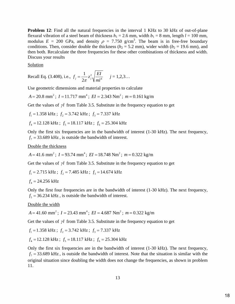
Problem 12: Find all the natural frequencies in the interval 1 KHz to 30 kHz of out-of-plane flexural vibration of a steel beam of thickness h1 = 2.6 mm, width b1 = 8 mm, length l = 100 mm, modulus E = 200 GPa, and density = 7.750 g/cm3. The beam is in free-free boundary conditions. Then, consider double the thickness (h2 = 5.2 mm), wider width (b2 = 19.6 mm), and then both. Recalculate the three frequencies for these other combinations of thickness and width. Discuss your results
Solution
Recall Eq. (3.408), i.e., 24
1
2j j
EIf z
ml j = 1,2,3…
Use geometric dimensions and material properties to calculate 220.8 mmA ; 411.717 mmI ; 22.343 NmEI ; 0.161 kg/mm
Get the values of l from Table 3.5. Substitute in the frequency equation to get
1 1.358 kHzf ; 2 3.742 kHzf ; 3 7.337 kHzf
4 12.128 kHzf ; 5 18.117 kHzf ; 6 25.304 kHzf
Only the first six frequencies are in the bandwidth of interest (1-30 kHz). The next frequency,
7 33.689 kHzf , is outside the bandwidth of interest.
Double the thickness 241.6 mmA ; 493.74 mmI ; 218.748 NmEI ; 0.322 kg/mm
Get the values of l from Table 3.5. Substitute in the frequency equation to get
1 2.715 kHzf ; 2 7.485 kHzf ; 3 14.674 kHzf
4 24.256 kHzf
Only the first four frequencies are in the bandwidth of interest (1-30 kHz). The next frequency,
5 36.234 kHzf , is outside the bandwidth of interest.
Double the width 241.60 mmA ; 423.43 mmI ; 24.687 NmEI ; 0.322 kg/mm
Get the values of l from Table 3.5. Substitute in the frequency equation to get
1 1.358 kHzf ; 2 3.742 kHzf ; 3 7.337 kHzf
4 12.128 kHzf ; 5 18.117 kHzf ; 6 25.304 kHzf
Only the first six frequencies are in the bandwidth of interest (1-30 kHz). The next frequency,
7 33.689 kHzf , is outside the bandwidth of interest. Note that the situation is similar with the
original situation since doubling the width does not change the frequencies, as shown in problem 11.
18

14
Double the thickness and the with 283.2 mmA ; 4187.48 mmI ; 237.495 NmEI ; 0.645 kg/mm
Get the values of l from Table 3.5. Substitute in the frequency equation to get
1 2.715 kHzf ; 2 7.485 kHzf ; 3 14.674 kHzf
4 24.256 kHzf
Only the first four frequencies are in the bandwidth of interest (1-30 kHz). The next frequency,
5 36.234 kHzf , is outside the bandwidth of interest. Note that the situation is similar with the
double the thickness situation since only the thickness influences the frequencies, as shown in Problem 11.
-------------------------------------
19
L3 10.9956078
L4 14.1371655 L5 17.2787597 L6 LL 6( ) L7 LL 7( )
fj
1
2 Lj 2
EI
m L4
f
j
1.358
3.742
7.337
12.128
18.117
25.304
33.689
103
-----------------------------
h 2 h1 b b1
A b h Ib h
3
12 EI E I m A
A 41.600 106
I 93.74 1012
EI 18.748 m 0.322
fj
1
2 Lj 2
EI
m L4
f
2.715
7.485
14.674
24.256
36.234
50.608
67.378
103
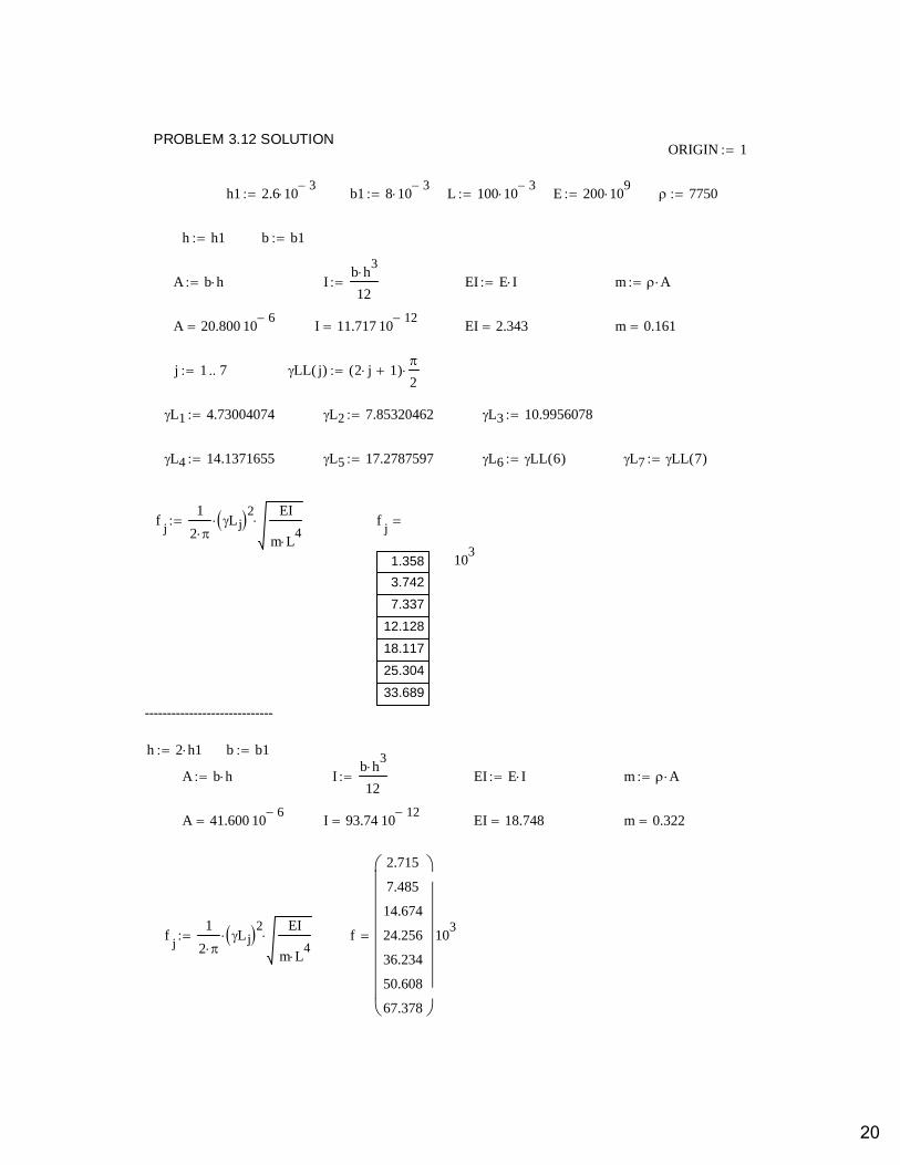
PROBLEM 3.12 SOLUTIONORIGIN 1
h1 2.6 103
b1 8 103
L 100 103
E 200 109
7750
h h1 b b1
A b h Ib h
3
12 EI E I m A
A 20.800 106
I 11.717 1012
EI 2.343 m 0.161
j 1 7 LL j( ) 2 j 1( )
2
L1 4.73004074 L2 7.85320462
20
f
2.715
7.485
14.674
24.256
36.234
50.608
67.378
103
fj
1
2 Lj 2
EI
m L4
m 0.645EI 37.495I 187.48 1012
A 83.200 106
m AEI E IIb h
3
12A b h
b 2 b1h 2 h1
--------------------------
f
1.358
3.742
7.337
12.128
18.117
25.304
33.689
103
fj
1
2 Lj 2
EI
m L4
m 0.322EI 4.687I 23.43 1012
A 41.600 106
m AEI E IIb h
3
12A b h
b 2 b1h h1
----------------------------
21
15
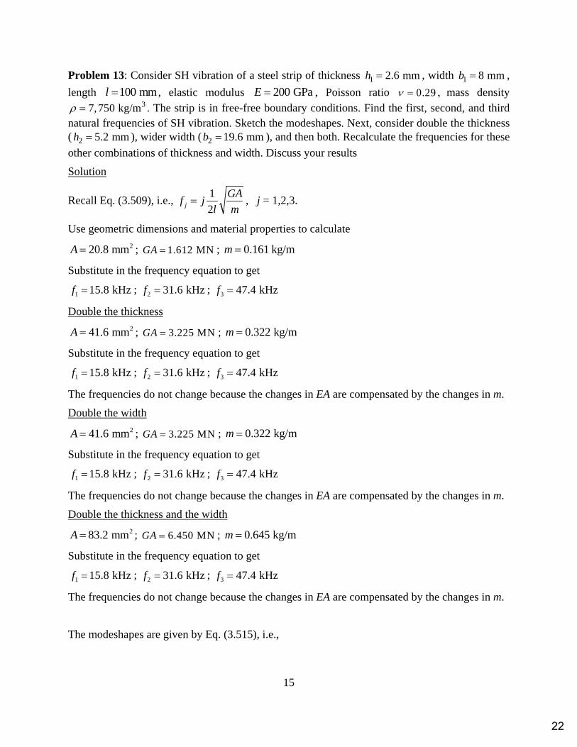
Problem 13: Consider SH vibration of a steel strip of thickness 1 2.6 mmh , width 1 8 mmb ,
length 100 mml , elastic modulus 200 GPaE , Poisson ratio 0.29 mass density 37,750 kg/m . The strip is in free-free boundary conditions. Find the first, second, and third
natural frequencies of SH vibration. Sketch the modeshapes. Next, consider double the thickness ( 2 5.2 mmh ), wider width ( 2 19.6 mmb ), and then both. Recalculate the frequencies for these
other combinations of thickness and width. Discuss your results
Solution
Recall Eq. (3.509), i.e., 1
2j
GAf j
l m , j = 1,2,3.
Use geometric dimensions and material properties to calculate 220.8 mmA ; 1.612 MNGA ; 0.161 kg/mm
Substitute in the frequency equation to get
1 15.8 kHzf ; 2 31.6 kHzf ; 3 47.4 kHzf
Double the thickness 241.6 mmA ; 3.225 MNGA ; 0.322 kg/mm
Substitute in the frequency equation to get
1 15.8 kHzf ; 2 31.6 kHzf ; 3 47.4 kHzf
The frequencies do not change because the changes in EA are compensated by the changes in m.
Double the width 241.6 mmA ; 3.225 MNGA ; 0.322 kg/mm
Substitute in the frequency equation to get
1 15.8 kHzf ; 2 31.6 kHzf ; 3 47.4 kHzf
The frequencies do not change because the changes in EA are compensated by the changes in m.
Double the thickness and the width 283.2 mmA ; 6.450 MNGA ; 0.645 kg/mm
Substitute in the frequency equation to get
1 15.8 kHzf ; 2 31.6 kHzf ; 3 47.4 kHzf
The frequencies do not change because the changes in EA are compensated by the changes in m.
The modeshapes are given by Eq. (3.515), i.e.,
22
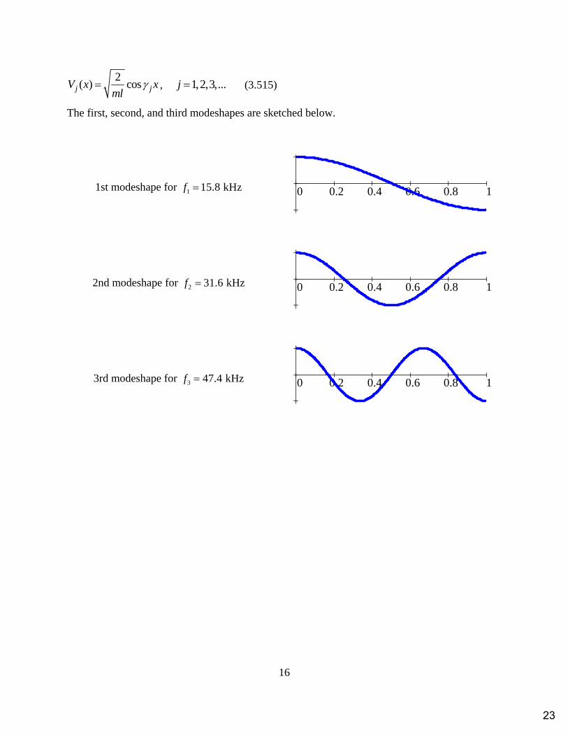
16
2( ) cosj jV x x
ml , 1,2,3,...j (3.515)
The first, second, and third modeshapes are sketched below.
1st modeshape for 1 15.8 kHzf
2nd modeshape for 2 31.6 kHzf
3rd modeshape for 3 47.4 kHzf
0 0.2 0.4 0.6 0.8 1
0 0.2 0.4 0.6 0.8 1
0 0.2 0.4 0.6 0.8 1
23
m 0.161
j 1 3
fj
j1
2 L
GA
m f
15.8
31.6
47.4
103
j 2 fj
j j
cS
------------------
h 2 h1 b b1
A b h GA G A m A
A 41.600106
GA 3.225 106
m 0.322
j 1 3
fj
j1
2 L
GA
m f
15.8
31.6
47.4
103
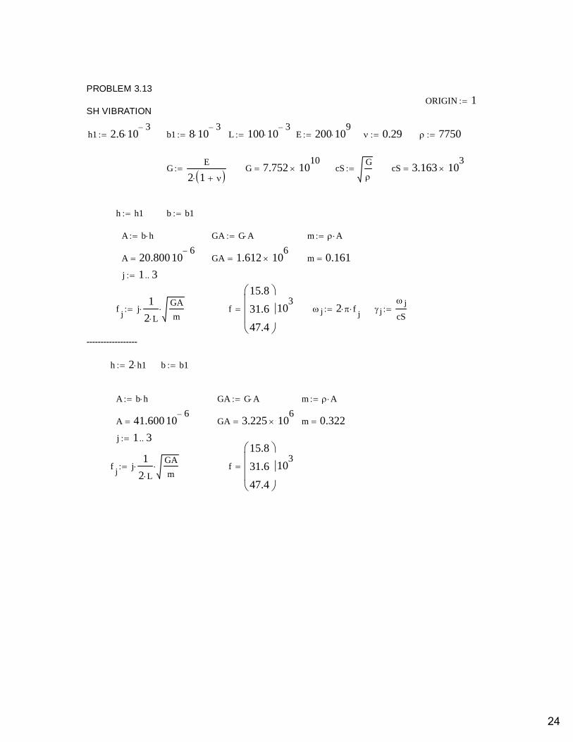
PROBLEM 3.13
SH VIBRATIONORIGIN 1
h1 2.6 103
b1 8 103
L 100 103
E 200 109
0.29 7750
GE
2 1 G 7.752 10
10 cS
G
cS 3.163 10
3
h h1 b b1
A b h GA G A m A
A 20.800106
GA 1.612 106
24
f
15.8
31.6
47.4
103
fj
j1
2 L
GA
m
j 1 3
m 0.645GA 6.450 106
A 83.200106
m AGA G AA b h
b 2 b1h 2 h1
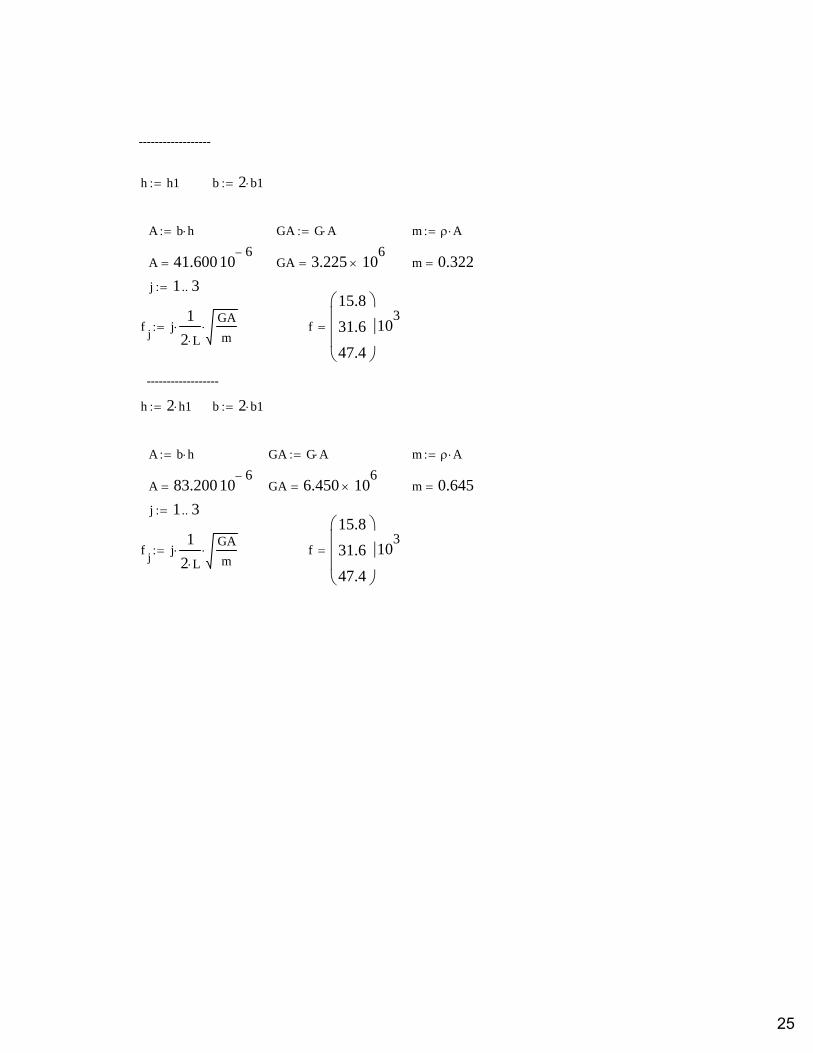
------------------
f
15.8
31.6
47.4
103
fj
j1
2 L
GA
m
j 1 3
m 0.322GA 3.225 106
A 41.600106
m AGA G AA b h
b 2 b1h h1
------------------
25

Nx 100 nx 1 Nx
xStart 0 xEnd L dxxEnd xStart
Nx 1 x
nxxStart nx dx
Vj nx cos j x
nx
26
17
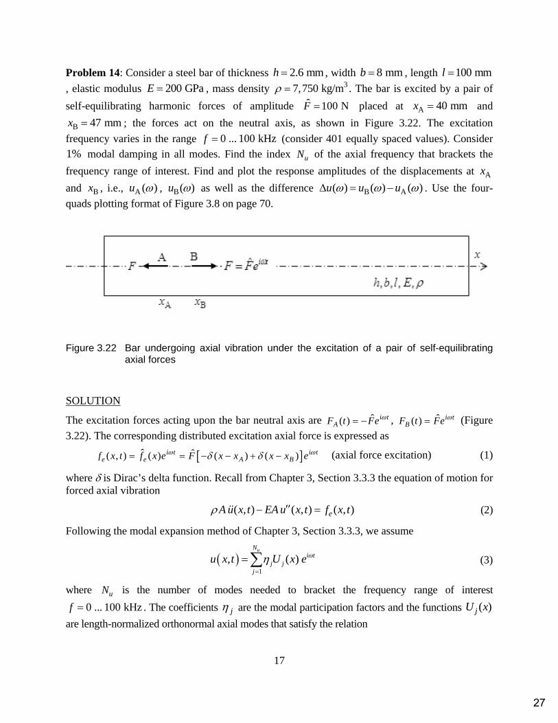
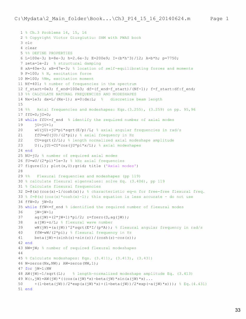
Problem 14: Consider a steel bar of thickness 2.6 mmh , width 8 mmb , length 100 mml , elastic modulus 200 GPaE , mass density 37,750 kg/m . The bar is excited by a pair of
self-equilibrating harmonic forces of amplitude ˆ 100 NF placed at A 40 mmx and
B 47 mmx ; the forces act on the neutral axis, as shown in Figure 3.22. The excitation
frequency varies in the range 0 ... 100 kHzf (consider 401 equally spaced values). Consider
1% modal damping in all modes. Find the index uN of the axial frequency that brackets the
frequency range of interest. Find and plot the response amplitudes of the displacements at Ax
and Bx , i.e., A ( )u , B( )u as well as the difference B A( ) ( ) ( )u u u . Use the four-
quads plotting format of Figure 3.8 on page 70.
Figure 3.22 Bar undergoing axial vibration under the excitation of a pair of self-equilibrating axial forces
SOLUTION
The excitation forces acting upon the bar neutral axis are ˆ( ) i tAF t Fe , ˆ( ) i t
BF t Fe (Figure
3.22). The corresponding distributed excitation axial force is expressed as
ˆ ˆ( , ) ( ) ( ) ( )i t i te e A Bf x t f x e F x x x x e (axial force excitation) (1)
where is Dirac’s delta function. Recall from Chapter 3, Section 3.3.3 the equation of motion for forced axial vibration
( , ) ( , ) ( , )eA u x t EA u x t f x t (2)
Following the modal expansion method of Chapter 3, Section 3.3.3, we assume
1
, ( )
uN
i tj j
j
u x t U x e (3)
where uN is the number of modes needed to bracket the frequency range of interest
0 ... 100 kHzf . The coefficients j are the modal participation factors and the functions ( )jU x
are length-normalized orthonormal axial modes that satisfy the relation
27

18
0
l
p q pqU U dx (4)
with pq being the Kronecker delta with the property 1pq for p q , and 0 otherwise.
For free-free beams, the length-normalized axial modeshapes can be calculated with the formulae given in Chapter 3, Section 3.3.2.1, Eqs. (3.256), (3.259), i.e.,
( ) cos( )j j jU x A x , 2
jAl
, j
j
l,
j j
E, 1,2,3,...j (5)
According to Chapter 3, Section 3.3.3.3, Eq. (3.295), the response by modal expansion is
i2 2
1
1, ( )
2
uNj t
jj j j j
fu x t U x e
A i (6)
where jf is the modal excitation calculated as
0
ˆ ( ) ( )l
j jf f x U x dx , 1, 2,3,...n (7)
Substitution of Eq. (1) into Eq. (7) yields
0
ˆ ˆ( ) ( ) ( ) ( ) ( ) l
j PWAS A B j PWAS j A j Bf F x x x x U x dx F U x U x (8)
In resolving Eq. (8), the localization property of the Dirac delta function was used, i.e.,
0 0( ) ( ) ( )x x f x dx f x (9)
Substitution of Eq. (7) into Eq. (6) yields the modal participation factor as
2 2
ˆ
2j B j A
jj j j
U x U xF
A i
, 1, 2, 3, ...j N (10)
Substitution of Eq. (10) into Eq. (3) followed by evaluation at Ax and Bx gives the amplitudes
1
ˆ( ) ;
uN
A A j j Aj
u u x U x (11)
1
ˆ ( ) ;
uN
B B j j Bj
u u x U x (12)
( ) B Au u u (13)
Note that substitution of Eqs. (10), (11), (12) into Eq. (13) and rearrangement yields
28
19
2 21
2
2 21
ˆ( )
2
ˆ
2
u
u
Nj B j A
B A j B j Aj j j j
Nj A j B
j j j j
U x U xFu u u U x U x
A i
U x U xF
A i
(14)
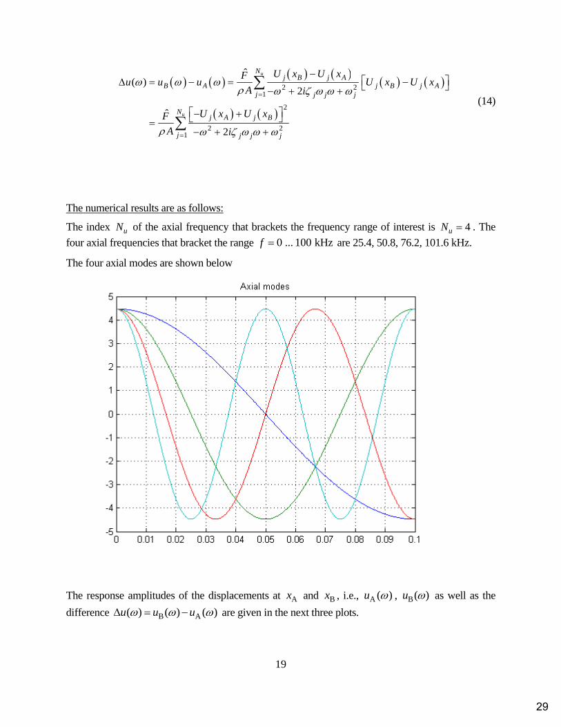
The numerical results are as follows:
The index uN of the axial frequency that brackets the frequency range of interest is 4uN . The
four axial frequencies that bracket the range 0 ... 100 kHzf are 25.4, 50.8, 76.2, 101.6 kHz.
The four axial modes are shown below
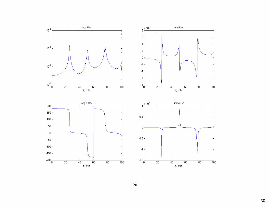
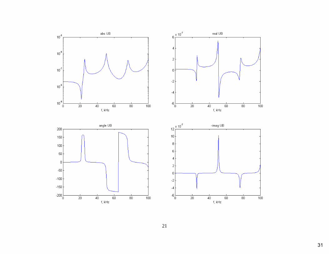
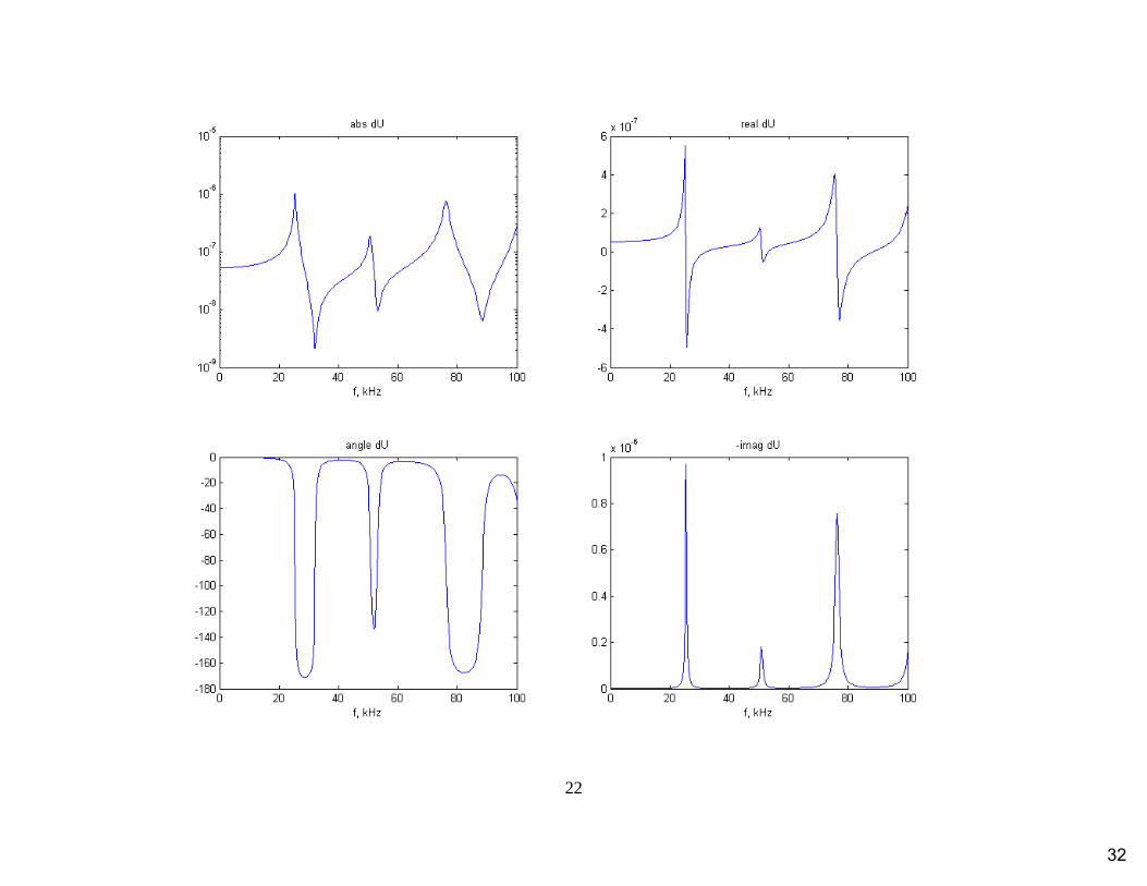
The response amplitudes of the displacements at Ax and Bx , i.e., A ( )u , B( )u as well as the
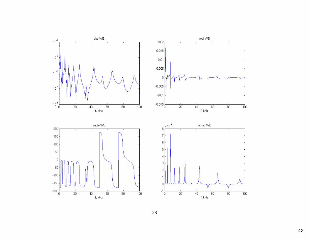
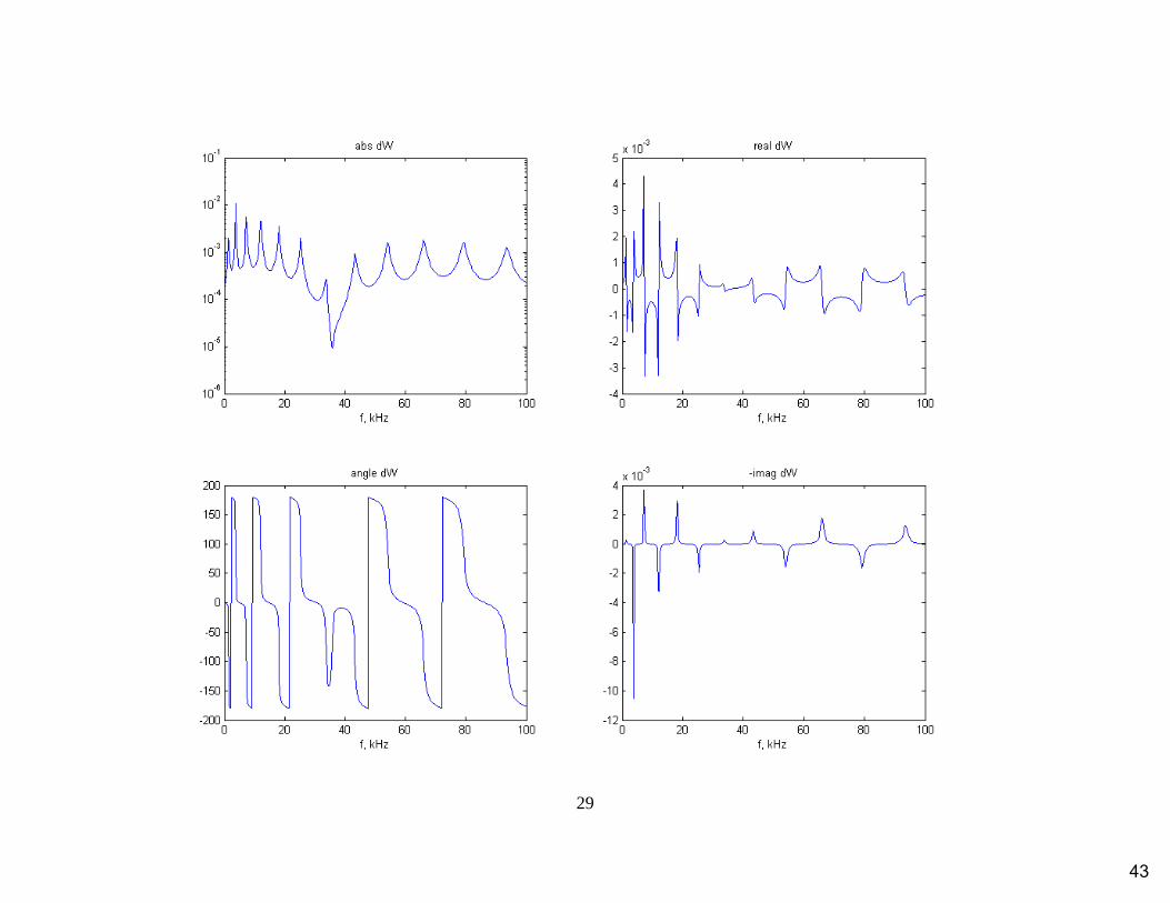
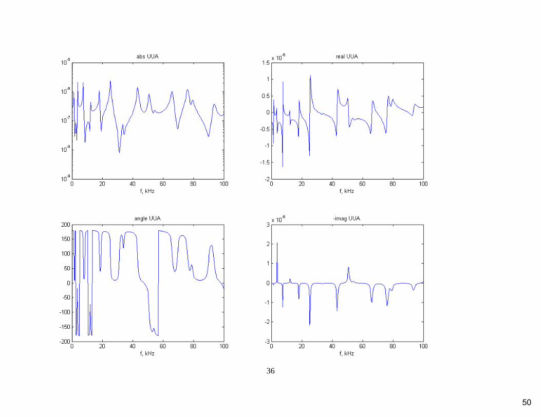
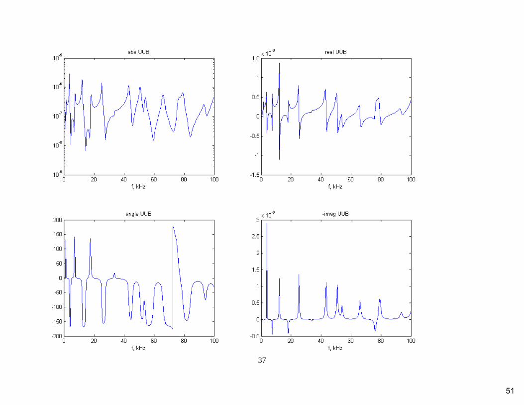
difference B A( ) ( ) ( )u u u are given in the next three plots.
29
20
30
21
31
22
32
33
34
35

36
23
Problem 15: Consider a steel beam of thickness 2.6 mmh , width 8 mmb , length
100 mml , elastic modulus 200 GPaE , mass density 37,750 kg/m . The beam is excited
by a pair of self-equilibrating harmonic moments of amplitude ˆ 100 N mM placed at
A 40 mmx and B 47 mmx , as shown in Figure 3.23. The excitation frequency varies in the
range 0 ... 40 kHzf (consider 401 equally spaced values). Consider 1% modal damping in all
modes. Find the index wN of the flexural frequency that brackets the frequency range of interest.
Find and plot the response amplitudes for displacements and slopes at Ax and Bx , i.e., A ( )w ,
A ( )w ; B( )w , B( )w ; as well as the differences B A( ) ( ) ( )w w w ,
B A( ) ( ) ( )w w w . Use the four-quads plotting format of Figure 3.8 on page 70.
Figure 3.23 Beam undergoing flexural vibration under the excitation of a pair of self-
equilibrating bending moments
SOLUTION
The excitation moments acting upon the beam are ˆ( ) i tAM t Me , ˆ( ) i t
BM t Me (Figure
3.23). The corresponding distributed excitation moment is expressed as
ˆˆ( , ) ( ) ( ) ( )i t i te e A Bm x t m x e M x x x x e (moment excitation) (15)
Recall from Chapter 3, Section 3.4.3.4, Eq. (3.461) the equation of motion for forced flexural vibration of a beam under distributed moment excitation, i.e.,
( , ) ( , ) ( , )eA w x t EI w x t m x t (16)
Assume the modal expansion
1
( , ) ( )
wN
i tj j
j
w x t W x e (17)
where N is the number of modes needed to bracket the frequency range of interest 0 ... 100 kHzf . The coefficients j are the modal participation factors and the functions
( )jW x are length-normalized orthonormal flexural modes that satisfy the relation
37

24
0
l
p q pqW W dx (18)
For free-free beams, the length-normalized flexural modeshapes can be calculated with the formulae given in Chapter 3, Section 3.4.2.1, Eqs. (3.409), (3.410) that dealt with vibration analysis, i.e.,
1( ) cosh cos sinh sinj j j j j jW x x x x x
l (19)
jj
z
l , 2
j jEI
A
, 1,2,3,...j (20)
with the eigenvalues jz and the modeshape factors j being given in Chapter 3, Table 3.5.
According to Chapter 3, Section 3.4.3.4, Eqs. (3.463), (3.464), the response by modal expansion is
i2 2
1
1, ( )
2j t
jj j j j
fw x t W x e
A i
(21)
where the modal excitation jf is given by
0
ˆ ( ) ( )l
j e jf m x W x dx , 1,2,3,...j (22)
Substitution of Eq. (15) into (22) gives
0 0
ˆˆ ( ) ( ) ( ) ( ) ( )l l
j e j A B jf m x W x dx M x x x x W x dx (23)
The r.h.s. of Eq. (23) can be simplified through integration by parts, i.e.,
0 0 00
l l
j jx x W dx x x W 0 00( )
l
j jx x W dx W x (24)
Hence,
0
( ) ( )l
A B j j A j Bx x x x W dx W x W x (25)
Substitution of Eq. (25) into Eq. (23) yields
ˆ ( ) ( )j j A j Bf M W x W x (26)
Substitution of Eq. (26) into Eq. (21) yields the modal participation factor as
2 2
ˆ ( ) ( )
2
j B j Aj
j j j
W x W xM
A i
(27)
Substitution of Eq. (27) into Eq. (17) followed by evaluation at Ax and Bx gives the amplitudes
38
25
1
ˆ( ) ; ( )
wN
A A j j Aj
w w x W x (28)
1
ˆ( ) ; ( )
wN
B B j j Bj
w w x W x (29)
( ) ( ) ( )B Aw w w (30)
Differentiation of Eq. (17) w.r.t. x gives the amplitude ˆ ( )w x as
1
ˆ ( ) ( )
wN
j jj
w x W x (31)
Evaluation of Eq. (31) at Ax and Bx yields
1
ˆ( ) ; ( )
wN
A A j j Aj
w w x W x (32)
1
ˆ( ) ; ( )
wN
B B j j Bj
w w x W x (33)
( ) ( ) ( )B Aw w w (34)
Note that substitution of Eqs. (27), (32), (33) into Eq. (34) and rearrangement yields
2 2
1
2
2 21
ˆ ( ) ( )( ) ( ) ( ) ( ) ( )
2
ˆ ( ) ( )
2
w
w
Nj B j A
B A j B j Aj j j j
Nj B j A
j j j j
W x W xMw w w W x W x
A i
W x W xM
A i
(35)
The numerical results are as follows:
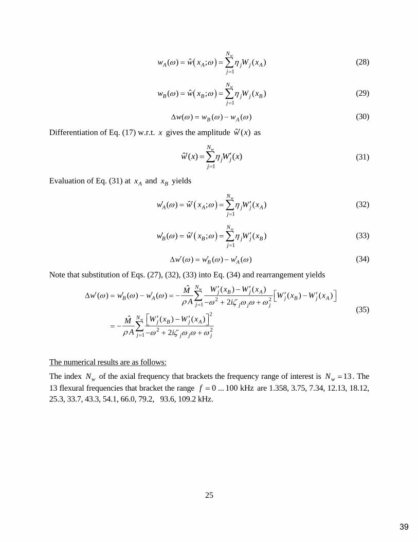
The index wN of the axial frequency that brackets the frequency range of interest is 13wN . The
13 flexural frequencies that bracket the range 0 ... 100 kHzf are 1.358, 3.75, 7.34, 12.13, 18.12, 25.3, 33.7, 43.3, 54.1, 66.0, 79.2, 93.6, 109.2 kHz.
39
26
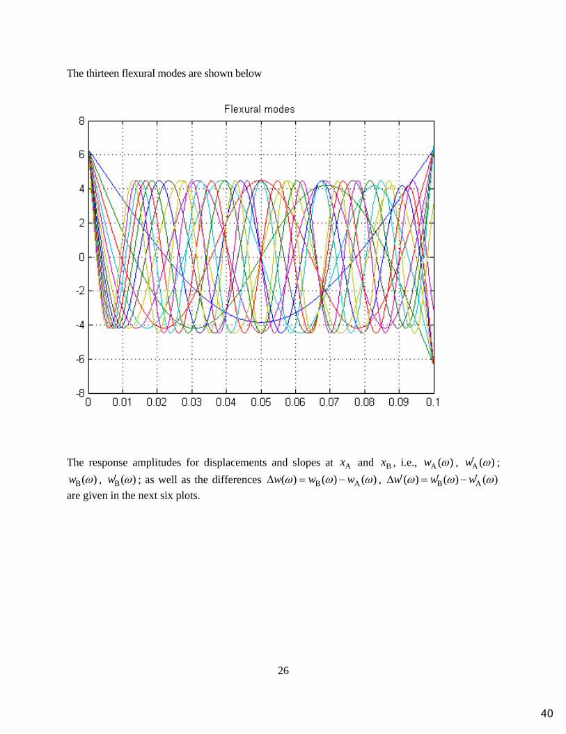
The thirteen flexural modes are shown below
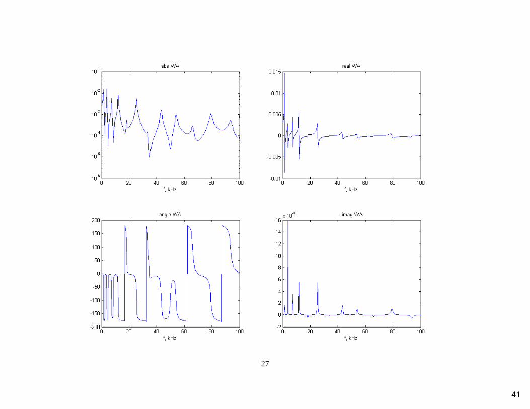
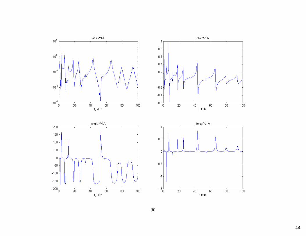
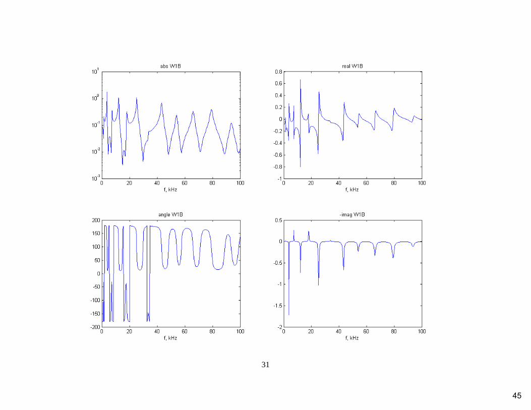
The response amplitudes for displacements and slopes at Ax and Bx , i.e., A ( )w , A ( )w ;
B( )w , B( )w ; as well as the differences B A( ) ( ) ( )w w w , B A( ) ( ) ( )w w w
are given in the next six plots.
40
27
41
28
42
29
43
30
44
31
45
32
46
33
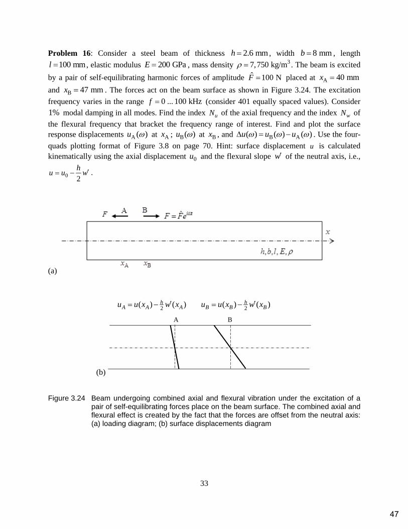
Problem 16: Consider a steel beam of thickness 2.6 mmh , width 8 mmb , length
100 mml , elastic modulus 200 GPaE , mass density 37,750 kg/m . The beam is excited
by a pair of self-equilibrating harmonic forces of amplitude ˆ 100 NF placed at A 40 mmx
and B 47 mmx . The forces act on the beam surface as shown in Figure 3.24. The excitation
frequency varies in the range 0 ... 100 kHzf (consider 401 equally spaced values). Consider
1% modal damping in all modes. Find the index uN of the axial frequency and the index wN of
the flexural frequency that bracket the frequency range of interest. Find and plot the surface response displacements A ( )u at Ax ; B( )u at Bx , and B A( ) ( ) ( )u u u . Use the four-
quads plotting format of Figure 3.8 on page 70. Hint: surface displacement u is calculated kinematically using the axial displacement 0u and the flexural slope w of the neutral axis, i.e.,
0 2
hu u w .
(a)
(b)
2( ) ( )h
B B Bu u x w x 2( ) ( )hA A Au u x w x
A B
Figure 3.24 Beam undergoing combined axial and flexural vibration under the excitation of a pair of self-equilibrating forces place on the beam surface. The combined axial and flexural effect is created by the fact that the forces are offset from the neutral axis: (a) loading diagram; (b) surface displacements diagram
47
34
SOLUTION
The excitation forces acting upon the beam surface can be reduced at the neutral axis into a pair of axial forces ˆ( ) i t
AF t Fe , ˆ( ) i tBF t Fe and a pair of bending moments ˆ( ) i t
AM t Me , ˆ( ) i t
BM t Me where
ˆ ˆ2
hM F (36)
The corresponding distributed excitation axial force and bending moment are expressed as
ˆ ˆ( , ) ( ) ( ) ( )i t i te e PWAS A Bf x t f x e F x x x x e (axial force excitation) (37)
ˆˆ( , ) ( ) ( ) ( )i t i te e A Bm x t m x e M x x x x e (moment excitation) (38)
where is Dirac’s delta function. As shown in Figure 3.24b, the neutral axis displacements ˆ( )Au x , ˆ( )Bu x and ˆ ( )Aw x , ˆ ( )Bw x combine to give the surface displacements Au , Bu according
to the kinematic formula
ˆ ˆ( ) ( )
2
ˆ ˆ( ) ( )2
A A A
B B B
hu u x w x
hu u x w x
(39)
The modal participation factors for axial and flexural motions are calculated by substituting Eqs. (36), (37), (38) into Eqs. (10), (27) to get
2 2
ˆ
2u u
u
u u u
j B j Aj
j j j
U x U xF
A i
, 1, 2, 3, ...u uj N (40)
2 2
ˆ ( ) ( )
2 2w w
w
w w w
j B j Aj
j j j
W x W xh F
A i
, 1, 2, 3, ...w wj N (41)
where the subscripts u and w signify axial and flexural modes, respectively. Substitution of Eqs. (40), (41) into Eq. (39) gives
1 1
( )2
u w
u u w w
u w
N N
A j j A j j Aj j
hu U x W x
(42)
1 1
( )2
u w
u u w w
u w
N N
B j j B j j Bj j
hu U x W x
(43)
Substitution of Eqs. (11), (12),(32), (33) into Eqs. (42), (43) yields
2
2 2 2 21 1
ˆ ˆ ( ) ( )( )
22 2
u wu u w w
u w
u wu u u w w w
N Nj B j A j A j B
A j A j Aj jj j j j j j
U x U x W x W xF h Fu U x W x
A Ai i
(44)
48
35
2
2 2 2 21 1
ˆ ˆ ( ) ( )( )
22 2
u wu u w w
u w
u wu u u w w w
N Nj B j A j A j B
B j B j Bj jj j j j j j
U x U x W x W xF h Fu U x W x
A Ai i
(45)
Subtraction of Eq. (44) from Eq. (45) yields
2 2
1
2
2 21
ˆ
2
ˆ ( ) ( )( ) ( )
2 2
uu u
u u
u u u u
ww w
w w
w w w w
Nj A j B
B A j B j Aj j j j
Nj A j B
j B j Aj j j j
U x U xFu u u U x U x
A i
W x W xh FW x W x
A i
(46)
Upon rearrangement, Eq. (46) yields
2 22
2 2 2 21 1
( ) ( )ˆ( )
22 2
u wu u w w
u wu u u w w w
N Nj B j A j B j A
j jj j j j j j
U x U x W x W xF hu
A i i
(47)
The numerical results are as follows:
The indices uN of the axial frequency and wN of the flexural frequency that bracket the
frequency range of interest are 4uN and 13wN .
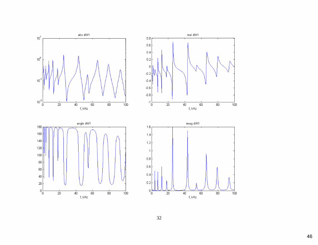
The surface response displacements A ( )u at Ax ; B( )u at Bx , and B A( ) ( ) ( )u u u
are given in the next three plots.
49
36
50
37
51

38
52
Recommended