15.1

Chapter 15Mode Split

In th is chapt er , the t h ird m odeling st ep in the crim e t ravel demand m odel isdis cussed, m ode split . Mode split in volves separa t in g (split t in g) t he predict ed t r ips fromeach or igin zone to each dest ina t ion zone int o dist inct t r avel modes (e.g., walk ing, bicycle,dr ivin g, t r a in , bus).

This model h as both adva ntages and disadva ntages for cr im e ana lysis . At atheoret ical level, it is t he m ost developed of the four st ages sin ce ther e h as been ext en siveresear ch on t ra vel mode choice. For crime an alysis, on t he oth er ha nd, it r epresents t he‘weakest link’ in the ana lysis sin ce there is very lit t le ava ilable in format ion on t ravel m odeby offender s. Since researchers can not int erview the gener a l public in order to documentcr imes committ ed by responden ts n or , in most cases, even in terview offender s a ft er theyhave been caught , th ere is very lit t le in format ion on t ravel mode by offender s t ha t has beencollected.1 Con sequent ly, we have to depend on the exist in g t heory of t r avel m ode choiceand adapt it in tu it ively to cr im e da ta . The approach is solely theoret ica l a nd depends onthe va lidit y of th e exist ing theory a nd on the in tu it iveness of guesses. H opefully, in thefu ture, th ere will be more informat ion collected t ha t would a llow the model to be ca libra tedagainst some r ea l da ta . But , for the t ime being, we are limited in wh at can be done.

Theoret ica l Backgroun d

Th e t heoret ical backgr oun d beh ind t he m ode split modu le is pr esen ted firs t . Next ,the specific procedures a re discussed wit h the model bein g illust ra ted wit h da ta fromBa lt imore County.

Util ity of Trave l and Mode Choice

The key a im of mode choice ana lysis is t o dist ingu ish the t r avel mode t ha t t r aveler s(or , in the case of cr im e, offenders) use in t r aveling between an or igin loca t ion and adest ina t ion loca t ion . In t he t r avel dem and m odel, th e choice is for t r avel between apar ticular origin zone an d a pa rt icular destinat ion zone. Thus, the t rips th at ar edis t r ibu ted from each origin zone t o each dest ina t ion zone in the t r ip d ist r ibu t ion modulear e fur th er split int o distinct t ra vel modes.

With few excep t ion s, t he assumpt ion beh in d the mode split decis ion is for a two-wa yt r ip. Th a t is, if an offender decides on dr iving to a par t icula r crim e loca t ion , we n orm allyassume tha t th is person will a lso dr ive ba ck to the or igin loca t ion . Sim ila r ly, if theoffender t akes a bus to a cr ime loca t ion , then tha t person will a lso t ake the bus back to theorigin locat ion . Ther e a re, of course, except ions. A car th ief ma y take a bus t o a cr imeloca t ion , then s tea l a ca r and d r ive back . But , in genera l, withou t in format ion to thecon t ra ry, it is a ssumed tha t the t r avel mode is for a round t r ip journey.

15.2

Un der lying the choice of a t r avel mode is a ssu med t o be a utility fun ction . This is afunct ion tha t descr ibes the benefit s and cos t s of t r avel by tha t mode (Or tuzar andWillumsen , 2001). This can be wr it t en wit h a conceptua l equa t ion :

Ut ility = F(benefits, costs) (15.1)

wh er e ‘f’ is some fun ction of the ben efits and t he cost s. Th e ben efits have to do wit h theadva ntages in t r aveling t o a par t icu la r dest in a t ion from a par t icu la r or igin while the cost shave to do wit h the r ea l and per ceived cost s of usin g a pa r t icula r mode. Sin ce th e ben efitsof t r aveling a par t icu la r des t ina t ion from a par t icu la r or igin a re p robably equa l, thedifferences in u t ility between t ravel modes essen t ially repr esen t differences in cost s. Thu s,equa t ion 15.1 breaks down to:

Ut ility cost = F(costs) (15.2)

If differen t t r avel m odes (e.g., dr iving, bik ing, wa lking) ar e ea ch r epresen ted by asepa ra te u t ility cost funct ion , th en they can be compa red:

Ut ilit y cost 1 = F 1(cost 1 + cos t 2 + cos t 3 + .....+cost k) (15.3a

Ut ilit y cost 2 = F 2(cost 1 + cos t 2 + cos t 3 + .....+cost k) (15.3b)

Ut ilit y cost 3 = F 3(cost 1 + cos t 2 + cos t 3 + .....+cost k) (15.3c)

.

.

.Ut ilit y cost L = F L(cost 1 + cos t 2 + cos t 3 + .....+cost k) (15.3d)

where Utility cost 1 th rough Ut ility cost L represent s L distinct t ra vel modes, cost 1th roughcost k r ep resen t k cost component s an d ar e var iables, an d F1 t h rough FL r ep resen t Ldifferen t u t ilit y fu nct ion s (one for ea ch mode).

Ther e a re sever a l obser vat ions t ha t can be m ade about th is r epresen ta t ion . Fir st ,each of the cost componen ts can be applied to a ll modes. However, t he cost componen ts a reva r ia bles in tha t the va lu es may or may n ot be the same. F or exa mple, if cost 1 is theoper a t ing cost of t r aveling from an or igin t o a dest ina t ion , th e cost for a dr iver is, of course,a lot h igher than for a bus pa ssen ger s ince th e lat t er per son sh ares t ha t cost with otherpassengers. Sim ila r ly, if cost 2 is the t r avel t im e from a par t icu la r or igin zon e to apa r t icu lar dest ina t ion zone, th en t ravel by priva te au tomobile may be a lot quicker than bypublic bus. As ment ion ed in the la st chapter , t im e differences can be conver ted in to cost sby a pplyin g some type of hour ly wage/pr ice to the t im e. To take one more exa mple, fordr ivin g m ode, t here could be a cost in parkin g (e.g., in a cen t ra l busin ess dis t r ict ); fort ransit use, on the other hand, t h is cost component is zero. In other words, each of thet ravel m odes has a differen t cost st ructure. The same cost s can be enumera ted, bu t someof them will n ot a pp ly (i.e., th ey h ave a va lue of 0).

15.3

Second, t he cost s can be per ceived cost s a s well a s r ea l cost s. F or example, anumber of studies have demonst ra ted tha t pr iva te au tomobile is seen as fa r moreconven ien t to mos t peop le than a bus or t r a in (e.g., see Schnell, Smith , Dimsda le, andTh rash er , 1973; Roemer and S inha , 1974; WASH COG, 1974; Carnegie-Mellon U niver sit y,1975; J ohnson, 1978; Levine and Wachs, 1986b). ‘Convenience’ is defined in t erms of easeof access and effor t in volved in t r avel (e.g., how lon g it t akes to walk to a bus stop from anor igin loca t ion , the number of t r ans fer s tha t have to made to reach a fina l des t ina t ion , andthe t ime it t akes to walk from the la st bus s top to th e fina l des t ina t ion). While it issomet imes difficu lt t o sepa ra te the effect s of convenience from t ravel itself, it is clear tha tmost people per ceive th is as dim ension in t r avel choice. In t u rn , convenience can beconver ted in to a moneta ry va lu e in order to a llow it to be ca lcu la ted in a cost equa t ion , forexa mple how much people a re willing t o pay in t im e savings to yield an equiva len t amountof conven ience (e.g., asking how many more m inutes in t r avel t ime by bu s a n individua lwould be willing to absorb in order to give up h aving to dr ive).

Thir d, t hese cost s can be considered a t an aggrega te as well as in dividua l level. Atan aggregat e level, they repr esen t avera ge or median cost s (e.g., th e avera ge time it t akesto t r avel between zon e A and zon e B by pr iva te au tomobile, bus, t r a in , wa lk in g, or bikin g; the average dolla r va lu e assigned by a sample of survey r espondents to the conveniencethey a ssocia te in t r avelin g by car as opposed to bus).

On the other hand, a t an individua l level, t he cost s a re specific to the in dividua l. For exa mple, t r avel t ime differ en ces bet ween car and bu s can be conver ted in to an hour lywage usin g th e individua l’s income; someone makin g $100,000 a yea r is going to pr ice tha tt ime savings d iffer en t ly than someone m aking only $25,000 a yea r .

Four th , a m ore cont rovers ial poin t , th e specific mathemat ica l funct ion tha t t ies thecos t s together in to a par t icu la r u t ility funct ion may a lso d iffer . Typ ica lly, mos t t r aveldem and m odels h ave assumed t ha t a similar mathemat ica l funct ion is used for a ll t r avelmodes; th is is the nega t ive exponent ia l fu nct ion descr ibed below (Domencich andMcFa dden , 1975; Ort uzar an d Willum sen , 2001). However, th ere is n o rea son whydifferen t funct ion s cannot be used. Thus, t he equa t ion s above iden t ify differen t funct ion sfor t he modes, F 1 t h rough F L. One can th in k of th is in terms of weights . Each of thedifferen t mathem at ical function weigh t the cost componen ts d iffer en t ly.

It is an empir ica l quest ion whether in dividua ls apply differen t funct ion s toevalua t ing the differen t modes. For exam ple, most people would not dr ive just to t r avelone block (un less it was pour ing ra in or u n less a heavy object had t o be delivered or pickedup). Even though it is conven ien t to get in to a veh icle and dr ive the one block, most peoplesee t he effor t involved (and, m ost likely, t he fuel a nd oil cost s) a s n ot bein g worth it .

In other words, it a ppea rs t ha t a differen t u t ility funct ion is being applied towa lking as opposed to dr iving (i.e., walk for dis t ances u p t o a cer t a in dis t ance; dr ivether ea fter ). A st r ict u t ilit y theorist might disagree with th is in ter pr et a t ion saying tha t theper minute cost of wa lking the one block and ba ck wa s les s t han monet a r ized per minutecost of opera t in g t he veh icle (which may inclu de openin g a ga rage door , get t in g in to the

15.4

veh icle, st a r t ing the veh icle, dr iving out of the parking spot, closing the ga rage door , andthen dr iving the one block). In oth er words , it cou ld be a rgued tha t the differ en ce inbehaviors h as t o do with the values of the differen t cost componen ts, ra ther than the waythey ar e weighted toget her (th e m athem at ical function). In ret rospect, one can expla inany difference. We argu e in th is chapter , h owever , t ha t cr im e t r ips appear to showdifferen t likelihoods by t ravel mode and tha t t r ea t ing each of these funct ions as d is t incta llows m ore flexibilit y in the framework .

Disc rete Choice Ana lysis

No mat ter how the u t ilit y fu nct ion s a re defin ed, t hey h ave to be combin ed in such away a s to a llow a discrete choice. Tha t is , a n offender in t r aveling fr om zon e A to zon e Bmakes a discrete choice on t ravel m ode. There may be a probabilit y for t r avel by eachmode, for exa mple 60% by ca r and 40% by bus. But , for an in dividua l, the choice is car orbus, n ot a probabilit y. Th e probabilit ies a re obt a in ed by a sample of in dividua ls , forexam ple of 10 individua ls 6 went by car an d 4 went by bus. But , still , at th e individua llevel, there is a d ist inct choice tha t was m ade.

Multinomia l Logi t Funct ion

A common mathemat ica l framework tha t used is for mode choice modeling a t anaggregat e level is t he m ultinom ial logit function (Domincich and McFadden , 1975; St oph erand Meyburg, 1975; Oppenheim , 1980; Or tuza r and Willumsen , 2001):

e (-$CijL

)

P ijL = -------------- (15.4) P

E[ e (-$CijL]

L=1

where P ijL is t he probability of us ing a mode for any pa r t icula r t r ip pa ir (par t icula r originand par t icula r dest ina t ion) L is the t r avel m ode, C ij is the cost of t r aveling fr om or igin zon e

i to dest ina t ion zone j, e is th e base of th e nat ur al logar ithm , an d $ is a coefficien t .

Severa l obser vat ions can be made a bout th is funct ion . Fir st , each t ravel mode, L,has it s own costs and benefit s, a nd can be eva lu a ted by it self. Th a t is , t here is a dis t in ct

u t ilit y fun ction for ea ch m ode. Th is is the n umer a tor of th e equa t ion, e (-$CijL

). However ,

the choice of any one mode is dependent on it s u t ilit y va lu e rela t ive to other modes (theden omina tor of the equa t ion). The m ore choices t ha t a re available, obviously, the lesslikely an in dividua l will u se tha t mode. But the va lu e associa ted wit h the mode (theu t ilit y) does not change. As ment ion ed above, we genera lly a ssume tha t the benefit oft raveling between any two zones is iden t ica l for a ll modes a nd, hen ce, an y differences a redu e t o cost s.

15.5

Second, t he m athem at ical form is t he nega t ive exponen t ia l. The exponen t ia lfunct ion is a growth funct ion in wh ich growth occur s a t a const an t rate (either posit ive - gr owth , or nega t ive - decline). The use of the nega t ive exponent ia l a ssumes tha t the cost sa re r ela ted to th e likelih ood a s a fun ction tha t declines a t a const an t ra te. It is a ctu a lly a‘dis incent ive’ or ‘dis count ’ fun ction ra ther than a u t ilit y fun ction , per se. That is, as t hecost s in crease , the probabilit y of usin g tha t mode decrea ses, a ll oth er th ings bein g equ a l. St ill, for h is tor ica l r easons, it is st ill ca lled a u t ilit y fu nct ion .

Thir d, for any on e mode, t he tota l cos t is a logar it hmic fu nct ion of in dividua l cos t s:

Ut ilit y cost i = e (-$CijL

) (15.5)

Ln(Ut ility cost L) = C ijL = " + $1X1 + $2X2 + ......+ $kXk (15.6)

where C ijL is a cum ulat ive cost made u p of componen ts X1, X2 t h rough Xk , " is a const an t ,an d $1 t h rough $k a re coefficient s for the individua l cost componen ts. Thu s, we see tha t theu t ility function is a loglinea r model, as was seen in cha pt er 12. Th us, t he u t ility function isPoisson distr ibut ed, declining at a const an t rate wit h increasin g cum ula t ive cost s. Domincich and McFadden (1975) su ggest tha t the er ror t erms a re not Poisson dist r ibut ed,bu t skewed in a Weibul fu nct ion . As discussed in chapter 12, t here a re a va r iety ofdifferen t models t ha t incorpora te skewed er ror terms (negat ive binomia l, a simple linearcor rect ion of dispersion ) so th a t the Weibul is bu t one of a number of poss ible descrip tors . Never theless, t he mean u t ilit y is a Poisson-type funct ion .

Gene ralized Relative Ut i li ty Funct ion

On e can gener a lize th is fur ther to allow any type of ma them at ical function. Whilethe Poisson has a lon g h is tory a nd is widely used, a llowin g ot her non-linear funct ion sa llows grea ter flexibility. It is possible tha t individua ls apply differen t weigh ting sys t emsin eva lu a t in g differen t modes (e.g., a nega t ive exponent ia l for walk in g, bu t a lognormalfunct ion for d r iving). We cer ta in ly see wha t appear to be d ifferen t funct ions when theactu a l t r avel beh avior of individua ls a re exa mined (e.g., homeless in dividua ls don’t wa lkeverywhere even t hough t he cost of wa lking long dista nces is cheaper in t r avel t ime t hantak ing a bus2; people don’t dr ive or t ake a bu s for ver y sh ort dis t ances, say a block or t wo). Therefore, if we a llow tha t there are differen t t r avel funct ions for differen t modes, t henmore flexibilit y is possible t han by a ssuming a sin gle m athem at ical function .

We can , th erefore, writ e a gen eralized relative u tility function as:

FL(-$C i jL) IijL

P ijL = ------------------ = ----------------- (15.7) P P

E[F L(-$C ijL)] E[I ijL]L=1 L=1

15.6

wh er e t he t er ms a re t he same a s in 15.4 except the function , F L, is some fun ction tha t isspecific to th e t r avel mode, L. The numer a tor is defined as t he impeda nce of mode L int raveling between two zones i an d j, while the denomina tor is the su m of a ll impeda nces.

Notice tha t the r a t io of the cost fun ction for one m ode r ela t ive to th e t ota l cost s isa lso the ra t io of t he im pedance for mode L rela t ive the tota l impedance. The tota lim pedance was defin ed in chapter 14 as the dis in cen t ive to t r avel a s a funct ion ofsepa ra t ion (dist ance, tr avel t ime, cost ). We see t ha t the sh are of a pa r t icu lar mode,therefore, is the propor t ion of the tota l impedance of tha t mode. This share will va ry, ofcourse, with the degree of sepa ra t ion . For any given sepa ra t ion , th ere will usu a lly be adifferen t sh are for each mode. For example, at low sepa ra t ion between zones (e.g., zonestha t a re n ext to each other ), walking and biking are m uch m ore a t t ractive than taking abus or a t r a in a nd, perhaps even dr iving. At grea ter sepa ra t ion (e.g., zones t ha t a re 5miles a pa r t ), wa lking and bik ing are a lmost ir r eleva nt choices and t he likelihood of dr ivingor u sing public tr an sit is mu ch great er. In oth er words, the sha re th at an y one modeoccupies is not cons tan t , bu t va r ies with the impedance funct ion .

Why th en can ’t we estima te t he m ode split directly at t he t rip distr ibut ion st age? Ifthe t r ip d ist r ibu t ion fun ction is

T ij = " P i8 $ Aj

J I ij (14.12 repea t )

and if these t r ips, in t u rn , ar e split int o dist inct m odes u sing equa t ion 15.7, cou ldn’t 14.12be re-wr itt en as

T ijL = " P i8 $ Aj

J I ijl (15.8)

where T ijL is t he n umber of t r ips bet ween two zones , i and j, by m ode L, P i is t he productioncapacity of zone i, Aj is t he a t t r action of zone j, " an d $ a re cons tan t s tha t a re applied to thepr oductions a nd a t t r actions r espectively, 8 an d J a re ‘fin e tun in g’ exponents of theproductions a nd a tt ra ctions r espectively, an d I ijL, is t he impeda nce of using mode L tot ravel between the two zones? Th e answer is , yes, it could be calcu la ted dir ect ly. If I ijL

was a per fect ly defined m ode impeda nce funct ion (with no er ror ), th en the mode sh arecou ld be ca lcu la ted direct ly a t the d is t r ibu t ion s tage ins tead of separa t ing the ca lcu la t ionsin to two d is t inct s t ages . The p roblem, however , is tha t the impedance funct ions a re neverper fect (fa r from it , in fact ) an d t ha t re-scalin g is r equ ired both to get the origin s a nddest ina t ions ba lanced in the t r ip d ist r ibu t ion st age and t o ensure t ha t the probabilit ies inequa t ion 15.7 add to 1.0. The effect of these adju stments genera lly t h rows off a model suchas 15.8.3 Consequ ent ly, th e t r ip dist r ibut ion and m ode sp lit st ages ar e usu a lly ca lcu lat edas separ at e operat ions.

Mea su ring Travel Costs

The next quest ion is wha t types of t r avel cos t s a re there tha t defin e im pedance? Asment ion ed above, t here a re rea l a s well as perceived cost s tha t a ffect a t r avel m ode

15.7

decision . Some of these can be m ea su red ea sily, wh ile oth er s a re ver y difficult requ ir ingdet a iled sur veys of individua ls. Among th ese cost s a re:

1. Dis tance or t r avel t im e. As ment ion ed th rough out th is discussion , d is t anceis on ly a rough indica tor of cost sin ce it is in var ian t wit h respect t o tim e. Actua l t r avel t ime is a much bet t er ind ica tor because it va r ies th roughoutthe day a nd can be easily con ver ted in to a t ravel tim e value, for exam ple bymultiplying by a un it wa ge.

2. Ot her rea l cost s, such a s t he oper a t ing cost s of a pr ivate veh icle (fuel, oil,maint enance), par kin g, and insu rance. Some of these can be subsu medunder t r avel t ime va lue by working ou t an hour ly pr ice for t r avel.

3. Perceived cost s, such as convenience, fea r of being caught by an offender ,ea se of escape from a crim e scene, difficult ies in moving s tolen goods , andfea r of reta lia t ion by other offen ders or ga ngs).

Some of these cost s can be measured and some cannot . F or exa mple, t he va lu e oft ravel t ime can be in ferred from the m edian househ old income of a zone for aggrega teana lysis or from the actua l househ old income for individua l-level an a lysis. Pa rkin g can beavera ged by zone. Insurance cost s can be est ima ted from zone avera ges if the da ta can beobtained.

Many perceived cost s a lso can be measu red. Convenience, for exam ple, cou ld bemeasured from a genera l survey. Th e fea r of bein g ca ugh t can be in fer red from the amountof su rveillance in a zone (e.g., the number of police per sonnel, secur ity guards , secur itycameras). Even though it may be a difficu lt en umera t ion pr ocess, it is s t ill possible tomeasu re these cost s a nd come up with some a vera ge estim ate.

Other per ceived cost s, on the other hand, may not be easily measu red. For example,the fea r an offender belon ging t o one ga ng h as about reta lia t ion from another ga ng is notea sily m ea su red. Sim ilar ly, th e cost s in moving st olen goods by a th ief is not ea silymea su red; one wou ld n eed to kn ow the loca t ion of th e dist r ibu tors of these goods .

In pract ice, t r avel m odeler s make sim ple assumpt ion s about cost s because of thedifficult y in mea su r ing many of th em . For exa mple, t r avel t ime is t aken as a pr oxy for a llthe opera t in g costs. P arkin g cost s can be in corpora ted th rough sim ple assumpt ion s aboutthe dist r ibu t ion a cross zones (e.g., zones wit h in the cen t ra l bu sin ess d ist ract - CBD, aregiven an average h igh pa rk ing cos t s; zones tha t a r e cen t r a l, bu t not in t he CBD, a reass igned moder a te parking cost s; zones t ha t a re subu rba n are a ss igned low pa rking cost s). It would be just too t ime consu ming to document each and every cost a ffect ing t ravelbeh avior , pa r t icula r ly if we a re developing a model of offender t r avel.

Never theles s, t heoret ically, t hese a re a ll poten t ia lly mea su rable cost s. They a rerea l a nd probably have an im pact in the t r avel decis ion s tha t offenders make. As

15.8

resea rcher s, we have to work towards a r t icula t ing as m any of th ese cost s a s possible inorder to p roduce a rea lis t ic represen ta t ion of offender t r avel.

Aggregate and Indiv idual Uti li ty Funct ions

One of th e big debat es in t ra vel modeling is wheth er to use aggregate or individua lu t ilit y fu nct ion s to ca lcu la te mode share. The aggrega te approach measures common cost sfor each zone, assuming an avera ge va lue. The d isaggregat e appr oach (somet imes ca lled‘second gener a t ion’ models) measures un ique cost s for individu a ls, then sums upwa rd t oyield va lu es for each zon e pa ir . E ven though the end resu lt is an a lloca t ion of cost s to eachzon e pa ir , t he a r t icu la t ion of un ique cost s a t the in dividua l level ca n , in theory, a llow amore rea list ic a ssessment of the u t ilit y fu nct ion tha t is applied to a region .

The aggrega te approach will m easure cost s by a verages. Thus, a typ ica l equa t ionfor dr iving mode m ight be:

Tota l cos t ij = " + $1T ij + $2 P j (15.9)

where T ij is th e avera ge tra vel time between two zones, i an d j, an d P ij is t he a ver agepa rking cost for pa rking in zone j. Notice th a t ther e a re a limited number of var iables inan aggrega te m odel (in t h is case, on ly two) and t ha t the a ss igned average is for an en t irezone. Not ice a lso tha t t he park ing cos t is applied on ly to the des t ina t ion zone. It isassumed tha t any t raveler will pay t ha t fee in tha t zon e ir respect ive of which or igin zon ehe/sh e came from.

A disaggregate appr oach can allow more cost component s, if th ey ar e measu red. Thus, a t ypica l equa t ion for dr iving mode m ight be:

Tota l cos t ijk = " + $1T ijk + $2 P j + $3C ijk + $4CM ijk + $5S ijk (15.10)

where T ijk is t he t r avel t ime for individua l k bet ween two zones , i and j, P ij is t he a ver agepa rking cost for pa rking in zone j, Cijk is the convenience of t r aveling to zone j from zone ifor individua l k , CMijk is t he comfor t and pr ivacy exper ienced by individua l k in t r avelingfrom zone i to zone j, and S ijk is t he per ceived sa fety exper ienced by individua l k int raveling fr om zon e i t o zon e j. N ot ice tha t there a re more cost va r ia bles in the equa t ionand t ha t the m odel is t a rget ed specifica lly to th e in dividua l, k . Two individua ls who livenext door t o each oth er an d who tr avel to th e same destinat ion m ay evalua te th esecomponents differen t ly. If these ind ividua ls have subs tan t ia lly d ifferen t incomes , then thevalue of the t r avel t ime will differ . If one values pr ivacy enorm ously while th e otherdoesn’t , then the cost of dr iving for the first is less than for the second. S imila r ly,conven ien ce is a ffected by both t r avel t ime a nd t he ea se of get t ing in and ou t of veh icle. F ina lly, th e per cept ion of sa fety ma y differ for these t wo hypothet ica l individu a ls. Ther eare m any st udies t ha t have documen ted the s ignifican t role pla yed by sa fety in a ffect ing,par t icu la r ly, t r ansit t r ips (Levine and Wa chs, 1986b).

15.9

In oth er words , the aggrega te approach applies a very elem en ta ry type of ut ilityfun ction wh er ea s t he disa ggrega te approach a llows much m ore complexity and in dividua lvar iabilit y. Of cour se , one has t o be able t o measu re t he in dividua l cost componen ts, adifficult t ask un der most circum sta nces.

Ther e is a lso a quest ion about wh ich a pproach is m ore a ccura te for cor rectlyforecas t ing actua l mode split s . His tor ica lly, mos t Met ropolit an P lann ing Organ iza t ionshave used the aggrega te method because it ’s easier . H owever , m ore recen t research(Domin cich and McFadden , 1975; Ben-Akiva and Lerman, 1985; McF adden , 2002) hassu ggest ed tha t the disa ggrega te m odeling may be m ore a ccura te. At the ver y minimum,the disa ggrega te is more amen able t o policy in ter pr et a t ions because it is m ore beh aviora l. If one could in terview t raveler s wit h a survey, then it is possible to explor e the va r iety ofcos t factor s t ha t a ffect a decis ion on both des t ina t ion and mode split , and a more r ea lis t ic(if not u n iqu e) ut ilit y fun ction der ived.

Bu t , as m en t ioned a bove, wit h crim e t r ips , th is is ver y difficu lt , if not impossible, t odo. Consequent ly, for the t im e bein g, we’re stuck wit h an aggrega te approach towardsmodeling the u t ility of t r avel by offender s.

Relative Access ibi li ty

For th is vers ion of Crim eS tat, an approxima t ion t o a u t ilit y fun ction wa s crea ted. The approach is to es t imate a relative accessibility funct ion and then app ly tha t funct ion tothe predict ed t r ip dis t r ibu t ion . The rela t ive accessibilit y fu nct ion is a mathemat ica lapproxima t ion t o a u t ilit y fun ction , ra ther than a mea su red u t ilit y fun ction by it se lf. Because the cos t components cannot be measured , a t leas t for offenders , we use anindu ctive a pproach. Reasonable a ssumpt ions a re m ade and a mathem at ical function isfoun d th at fits th ese assu mpt ions.

It is a pla usible model, not a n ana lyt ical one. The plausibility comes by makingreasonable assu mpt ions a bout actu al tr avel beha vior. One can assu me th at walking tr ipswill occu r for shor t t r ips, say u nder two miles. Bicycle t r ips, on the other hand, cou ld occurover lon ger dis t ances, bu t will s t ill be rela t ively shor t (a lso, t here is a lways the r isk oft ra ffic on the sa fety of bicycle t r ips). Transit t r ips (bus and t ra in ) will be used formoderat ely long dista nces but require an a ctu al tr an sit network . Finally, driving tr ips ar ethe m ost flexible becau se they can occur over any size dis t ance and r oad net work. They a reless likely to be used for very sh or t t r ips, on the other hand, due to reasons d iscussedabove.

Hierarch ical Approac h to Es timatin g Mode Acce ssibi l i ty

Usin g th is a pproach, specific st eps can be defined t o produce a p lausibleaccessibility model. To help in est ablishing a m odel, an Excel spr eadsh eet has beendeveloped for makin g t hese ca lcu la t ion s (Estim ate m ode split im pedan ce valu es.xls). I t cana lso be downloaded from t he Crim eS tat download pa ge. The spr eadsh eet has been definedwit h respect to dis t ance, bu t it can be adapted for any t ype of im pedance (t r avel t im e or

15.10

cost). A spreadsh eet h as been used becau se it is more flexible th an incorpora ting it a s arou t ine in Crim eS tat to est im ate the parameter s. There is not a sin gle solu t ion to thepa rameters est ima tes, an d t he differen t choices can be seen more easily in a spr eadsh eet .

D efi n e t a r g et p r op o r ti on s

Firs t , define t he m odes. In the Crim eS tat mode sp lit r ou t ine, up t o five differen tmodes a re a llowed. These h ave defau lt names of “Walk”, “Bike”, “Dr ive”, “Bu s”, and“Train”. The user is not r equired to use th ese na mes nor all five modes. Clearly, if th ereis not a t r a in system in t he st udy ar ea , th en the “Tra in” mode does not a pply. Travelmodeler s use var ia t ions on these, such as “dr ive a lone”,”carpool”, “au tomobile”,“motorcycle”, a nd so for th .

D efi n e t a r g et p r op o r ti on s

Second, define t he target proportions. These a re the expected pr oport ions of t r avelfor each mode. Wher e would su ch pr oport ions come from? Ther e have been m any studiesof dr iving and t ransit beh avior , bu t rela t ively few s tudies of bicycle and pedest r ian use(Turner , Shu nk, and H ot tenst ein, 1998; Schwa r tz et a l, 1999; Por ter , Suh rbier a ndSchwa r tz, 1999). Ther e are not simple tables tha t one can look u p defau lt va lues .

To solve th is p roblem, examples wer e sough t from differen t size met ropolitan a rea s. Est ima tes of t r avel mode sh are for a ll t r ip pu rposes (work a nd n on-work) were obta inedfrom1) Ot tawa (Ot tawa , 1997); 2) Por t la nd (Por t la nd, 1999); and Houston 4. Table 15.1sh ows t he es t imated sh ares. The H ouston da ta does n ot in clude wa lking and bik ingsha res, and tr an sit tr ips ar e not distinguished by mode in t he Port land an d Otta wa dat a.

Ta ble 15.1Est imated Mode Share for Three Metropoli tan Areas

Al l Tr ip Pu rposes

Ottaw a P o rt la n d Houston

P o p u la ti on : 725 thousand 2.0 million 4.6 million (1995) (2001) (2000)

Pe rcent o f trips by: (1995) (1994) (2025 forecast )Dr iving 73.5% 88.6% 98.3%Tr ansit 15.2% 3.0 1.7%

(bu s 1.1%; ra il 0.6%)Walking 9.6% 4.6% -Bicycle 1.7% 1.0% -Other - 2.8% -

Wh ile it ’s difficu lt to genera lize, wa lk in g is very m uch dependent on the existence ofan exten sive tr ansit syst em. In H oust on , th e t r ansit syst em is pr ima r ily a commuter

15.11

sys tem whereas in Por t la nd and Ot tawa , it serves mult ip le purposes. Clear ly, t he morecompact the u rban a rea , the more likely tha t t r ips will occur by t rans it , wa lk ing or bik ing. But , even in the case of Ot tawa where a lm ost 10% of t r ips a re by walk in g, the major it y oft r ips a re by pr ivate veh icle. In the United St a tes and Ca nada , for m et ropolitan a rea s withext ensive t r ansit facilit ies (New York, Chica go, Bos ton , Mont rea l), a major it y of r egiona lt r ips a re st ill by au tomobile.

Based on t h is, some defau lt va lues were selected a nd pu t int o the spr eadsh eet . Thesprea dsheet requ ires tha t they a re en ter ed as p ropor t ions (not per cent ages). The defau lt sva lu es were (table 15.2):

Ta ble 15.2D e fa u lt Mo de S h are Va lu e s

Propor t ionsMode Sh areWalk .04Bicycle .01Dr iving .90Bus .04Tr a in .01

The user can modify these in the spreadsheet . I t ’s im por tan t tha t a user contact theloca l Met ropolit an Pla nnin g Orga niza t ion to fin d out wha t would be reasonable va lu es forthe u rba n area . The defau lt va lues a re bu t guesses based on a limited amoun t of da ta .

An a lt erna t ive approach is to use the J ourney to Work da ta of the U.S . CensusBureau (2004). Dur in g every census, t he Census Bu reau documents home-to-work‘commute’ t r ips a nd br eaks down t hese da ta by mode share. They relea se t hese da ta underthe t it le “J our ney to Work ”. In the United St a tes in 2000, 87.9% of all h ome-to-work t r ipswer e by pr ivate veh icle (au tomobile, van , t ruck), 4.7% wer e by public tr ansit (bus 2.5%; ra il2.1%; other 0.1%), 2.9% were by walkin g, 0.4% were by bicycle, 0.1% were by motorcycle,0.7% were by other means, an d 3.3% worked a t home.

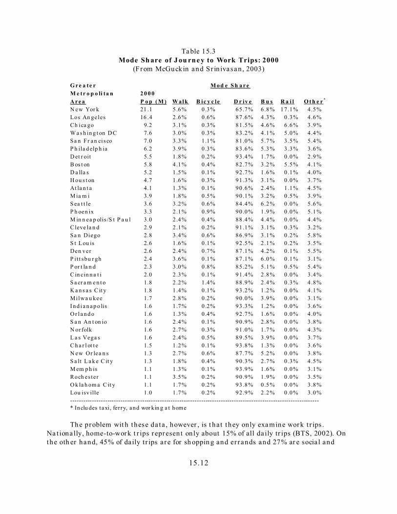
Nat iona l journey to work st a t ist ics for 1990 a nd 2000 a nd for met ropolitan a rea s in1990 can be foun d at h t tp://www.censu s.gov/popu la t ion/www/socdem o/journey.h tml. Dat aon met ropolita n a reas for 2000 can be found in McGuckin and Sr inivasan (2003). In 2000,the home-to-work m ode sh are for a sa mple of lar ge met ropolita n (including th e 15 lar gest )a reas is shown in Ta ble 15.3. They a re rank-ordered by the 2000 popula t ion of themet ropolit an a rea .

As can be seen , t he la rger met ropolit an a reas genera lly have a h igher sha re oft ransit use and walk in g t han smaller met ropolit an a reas, bu t the differences a re not tha tdr amat ic. Even the la rgest met ropolitan a rea s h ave a major ity of th eir home-to-work t r ipsby priva te vehicle.

15.12

Ta ble 15.3Mode Sh are of J ou rn e y to Work Trips: 2000

(From McGuckin and Sr in ivasan , 2003)

G r e a te r M o d e S h a r e

M e tr o p o li ta n 2 0 0 0

A r e a P o p ( M ) Walk B ic y c le D r iv e B u s R a i l O t h e r *

N ew Yor k 21 .1 5 .6% 0 .3% 65 .7% 6 .8% 17.1% 4 .5%

Los An geles 16 .4 2 .6% 0 .6% 87 .6% 4 .3% 0 .3% 4 .6%

Ch ica go 9.2 3 .1% 0 .3% 81 .5% 4 .6% 6 .6% 3 .9%

W a s h in g t on D C 7.6 3 .0% 0 .3% 83 .2% 4 .1% 5 .0% 4 .4%

Sa n Fr an ci sco 7.0 3 .3% 1 .1% 81 .0% 5 .7% 3 .5% 5 .4%

P h ila d elp h ia 6.2 3 .9% 0 .3% 83 .6% 5 .3% 3 .3% 3 .6%

D et r oit 5.5 1 .8% 0 .2% 93 .4% 1 .7% 0 .0% 2 .9%

B os t on 5.8 4 .1% 0 .4% 82 .7% 3 .2% 5 .5% 4 .1%

D a lla s 5.2 1 .5% 0 .1% 92 .7% 1 .6% 0 .1% 4 .0%

H ou s t on 4.7 1 .6% 0 .3% 91 .3% 3 .1% 0 .0% 3 .7%

At la n t a 4.1 1 .3% 0 .1% 90 .6% 2 .4% 1 .1% 4 .5%

M ia m i 3.9 1 .8% 0 .5% 90 .1% 3 .2% 0 .5% 3 .9%

S ea t t le 3.6 3 .2% 0 .6% 84 .4% 6 .2% 0 .0% 5 .6%

P h oen ix 3.3 2 .1% 0 .9% 90 .0% 1 .9% 0 .0% 5 .1%

M in n ea p olis /S t P a u l 3.0 2 .4% 0 .4% 88 .4% 4 .4% 0 .0% 4 .4%

C leve la n d 2.9 2 .1% 0 .2% 91 .1% 3 .1% 0 .3% 3 .2%

Sa n Diego 2.8 3 .4% 0 .6% 86 .9% 3 .1% 0 .2% 5 .8%

S t Lou is 2.6 1 .6% 0 .1% 92 .5% 2 .1% 0 .2% 3 .5%

Den ver 2.6 2 .4% 0 .7% 87 .1% 4 .2% 0 .1% 5 .5%

P it t sbu r gh 2.4 3 .6% 0 .1% 87 .1% 6 .0% 0 .1% 3 .1%

P or t la n d 2.3 3 .0% 0 .8% 85 .2% 5 .1% 0 .5% 5 .4%

C in cin n a t i 2.0 2 .3% 0 .1% 91 .4% 2 .8% 0 .0% 3 .4%

S a cr a m e n t o 1.8 2 .2% 1 .4% 88 .9% 2 .4% 0 .3% 4 .8%

K a n s a s C it y 1.8 1 .4% 0 .1% 93 .2% 1 .2% 0 .0% 4 .1%

Milwa u kee 1.7 2 .8% 0 .2% 90 .0% 3 .9% 0 .0% 3 .1%

I n d i a n a p o lis 1.6 1 .7% 0 .2% 93 .3% 1 .2% 0 .0% 3 .6%

O r l a n d o 1.6 1 .3% 0 .4% 92 .7% 1 .6% 0 .0% 4 .0%

S a n An t on io 1.6 2 .4% 0 .1% 90 .9% 2 .8% 0 .0% 3 .8%

N or folk 1.6 2 .7% 0 .3% 91 .0% 1 .7% 0 .0% 4 .3%

L a s Vega s 1.6 2 .4% 0 .5% 89 .5% 3 .9% 0 .0% 3 .7%

C h a r l ot t e 1.5 1 .2% 0 .1% 93 .8% 1 .3% 0 .0% 3 .6%

N ew Or lea n s 1.3 2 .7% 0 .6% 87 .7% 5 .2% 0 .0% 3 .8%

S a lt L a k e C it y 1.3 1 .8% 0 .4% 90 .3% 2 .7% 0 .3% 4 .5%

M em p h is 1.1 1 .3% 0 .1% 93 .9% 1 .6% 0 .0% 3 .1%

Roch es ter 1.1 3 .5% 0 .2% 90 .9% 1 .9% 0 .0% 3 .5%

O k la h om a C it y 1.1 1 .7% 0 .2% 93 .8% 0 .5% 0 .0% 3 .8%

Lou isv ille 1.0 1 .7% 0 .2% 92 .9% 2 .2% 0 .0% 3 .0%

------------------------------------------------------------------------------------------------------------------

* Inclu des taxi, fer ry, and wor kin g a t home

Th e problem wit h these da ta , however , is t ha t they only examine work t r ips . Na t iona lly, home-to-work t r ips represen t on ly about 15% of all da ily tr ips (BTS, 2002). Onthe oth er hand, 45% of da ily tr ips a re for sh oppin g and er rands and 27% ar e socia l and

15.13

recrea t iona l. Fur ther , non-work t r ips a re even more likely t o occur by au tomobile, and a regenera lly shor ter . F or exa mple, in Houston , for home-based non-work t r ips, on ly 1% oft r ips a re by t ransit compared to 3.1% for home-to-work t r ips. These home-based non-workt r ips may be a bet t er ana logy to cr ime t r ips than work t r ips sin ce th ey t en d t o be of similartr ips lengths a s crime tr ips.

Thus, u n less t he u ser is willin g to assu me t ha t a crim e t r ip is like a work t r ip(which is quest ionable), th en the J our ney to Work tables a re probably not t he bes t guidefor the ta rget propor t ion s. Never theless, a n exa min a t ion of them is va lu able to see howwork tr ips ar e split am ong the various t ra vel modes.

S el ec t m o d e fu n ct i on s

Third, select mathem at ical functions t ha t approximate accessibility ut ility. Again ,some plau sible assu mpt ions n eed to be made. In Crim eS tat, the u ser can select among fivedifferen t mathem at ical functions (linea r , nega t ive exponen t ia l, norm al, lognorm al,t runcated nega t ive exponent ia l). Th e defau lt funct ion s a re (Ta ble 15.4):

Ta ble 15.4D e fa u lt Mo de S h are F u n ct io n s

Mode Funct ionWalk Nega t ive exponen t ia lBicycle Nega t ive exponen t ia lDr iving Logn ormalBus Logn ormalTr a in Logn ormal

The reasoning behind th is is th at walking and biking are r elat ively short tr ips,whereas t r ansit modes a re used for in termedia te lengt h t r ips while dr ivin g ca n be used forany length t r ip. Th us, it ’s u n likely tha t an au tomobile will be u sed for very sh ort t r ips(less than a quar ter mile) an d it ’s ver y un likely tha t t r ansit will be u sed for sh ort t r ips(less t han a ha lf mile or more). Nevert heless, th e user can modify th ese choices a ndexam ine t he appr opr iat e colum n in t he spr eadsh eet .

S elect m od el p r ior it ies

Four th , select the pr ior it ies for modeling t he ta rget . Unfor tunately, t here may n otbe a s ingle solut ion tha t will yield the ta rget pr oport ions. Ther efore, a decision needs t o bemade on which o rd e r the spreadsheet will be calcu la ted. The defau lt order is (table 15.5 ):

15.14

Ta ble 15.5D e fa u lt Mo de S h are F u n ct io n s

Order ofMode IterationWalk 1Bicycle 2Dr iving 3Bus 4Tr a in 5

The r ea soning is t ha t the offender fir st makes a decision on t he len gth of the t r ip(sh or t , medium , long, or the equiva lent in t r avel t ime). Then , with in ea ch ca tegory, makesa decis ion on which mode to choose. F or very shor t t r ips, t he defau lt mode is walk in g. Forin ter media te t o long t r ips , the defau lt choice is d r iving. However , the u ser can cha nge th isorder .

It er a t i v el y es ti m a t e p a r a m e t er s

Fifth , in the spr eadsh eet , it era t ively adjus t the pa rameters u n t il the ta rgetpropor t ion is reached. Do th is in the order selected in the above step. Aga in , t here is not asin gle solu t ion tha t will produce t he ta rget propor t ion . F or example, each of thema th emat ical fun ctions h as t wo or t hr ee par am eters t ha t can be adjusted:

1. For the negat ive exponent ial, th e coefficient and exponent2. For the normal d is t r ibu t ion , t he mean dis t ance, s t andard devia t ion and

coefficient3. For lognormal d is t r ibu t ion , t he mean dis t ance, s t andard devia t ion and

coefficient4. For t he linear distr ibut ion, an int ercept an d slope5. For the t runca ted nega t ive exponent ia l, a peak dis t ance, peak likelihood,

in ter cept , and exponen t .

Th e t a rget pr oport ion can be a chieved by adju st ing any or a ll of the paramet er s. For example, to ach ieve a ta rget pr oport ion of 0.05 (i.e., 5%) usin g the n ega t iveexponent ial, an infin ite n umber of models can yield th is, for exam ple coefficient =0.0366,exponent=-2.63; coefficien t=0.0459 or exponent=-5; coefficien t=0.01966, exponent=-1; andso for th . Ther efore, th ere must be addit iona l cr iter ia t o const ra in t he choices.

On e crit er ia is t o set an approximate m ea n dis t ance. For example, with wa lkingt r ips, th e mean dist ance can be set to a ha lf mile or for dr iving, th e mean dist ance can beset to 6 m iles. Then , ch eck the approximate mean dis t ance of the selected funct ion .Though ra rely will t he exa ct mean dis t ance be replica ted, t he ca lcu la ted mean dis t ancesh ould be close to th e idea l. The one except ion is for very sh ort t r ips . Since th e in ter valsin t he spr eadsh eet a re a ha lf mile each , th ere is consider able err or for very sh or t dist ances.

15.15

Exa m in e th e gr a p h s in th e sp r ea d sh eet

Another is to examine the graph of the funct ion in the spreadsheet (below theca lcu la t ions ). Does the typ ica l t r ip approximate the expected mean d is tance? Does theselected funct ion pr odu ce somet h ing tha t looks int u itive? Adm itt edly, these a re su bject ivedecisions. But , if the funct ion looks st range, it can be caught and r e-ca lcu lat ed.

In sh or t , th e a im should be to produ ce a funct ion tha t not on ly capt ures t he ta rgetpr opor t ion , but looks plau sible. Severa l examples ar e shown below. Figure 15.1 shows t hedefau lt wa lking model usin g a nega t ive exponen t ia l. Figu re 15.2 shows t he defau lt bik ingmodel, a lso usin g a nega t ive exponent ia l. Figure 15.3 shows the defau lt dr ivin g m odeusin g a lognormal fun ction . Figure 15.4 shows t he defau lt bu s m ode, a lso usin g alognormal funct ion and figure 15.5 shows the defau lt t r a in mode us ing a lognormalfunct ion .

F igure 15.6 shows the cumulat ive resu lts of the defau lt va lues . This is a lso gra ph edin the spr ea dsheet , st a r t ing in cell I1. Notice h ow the r ela t ive a ccessibility fun ction works. As dista nce increases, the mode proport ions cha nge. At very short dista nces, walking tr ipspr edomina te with biking t r ips a lso gett ing a moder a te sh are. As t he dist ance increa ses,the propor t ions in creasin gly sh ift t oward dr iving. Even though the likelihood of dr ivingdeclines with dis t ance, the other modes decline even fas ter . In oth er words , the r ela t iveaccessibilit y fu nct ion is es t im at in g t he rela t ive shares of ea ch mode as a funct ion of theimpeda nce (in th is case , dis t ance).

Ad a p ti ng sp rea d sheet for t ra vel t im e or tr a vel cost

The illus t ra t ions t o th is poin t have used dist ance as a n impeda nce un it. However,oth er impeda nce unit s, such a s t r avel t ime a nd gener a lized t ravel cost , can a lso be u sed. These gener a lly require a network (see below) in t ha t weight s h ave to be ass igned t osegmen ts. Never theless, t he same logic applies . For ea ch t ravel mode, a specificimpeda nce function is est imated and t hen app lied to th e t r ip d ist r ibu t ion m at r ix.

Em p ir ica lly est im a ti ng th e m od e-sp ecific im p ed a nce

As ment ioned a t the beginn ing of th is chap ter , the lack of in format ion aboutoffender t r avel modes has necessit a ted the use of mathemat ica l ‘guesses ’ abou t t r avelbehavior . However , if it wer e possible to obta in a ctua l in format ion on t ravel modes byoffenders, t hen th is in format ion could be u t ilized dir ect ly to est im ate a much moreaccura te im peda nce function . If th is da tabase existed , th en two appr oaches a re possible:

1. F it the da ta wit h the va r ious m athem at ical functions t o see wh ich ones fitbest a nd t o estimat e the par am eters.

2. Use the ker nel densit y function to est imate a non-linea r impeda nce valu ewit h the specific in format ion .

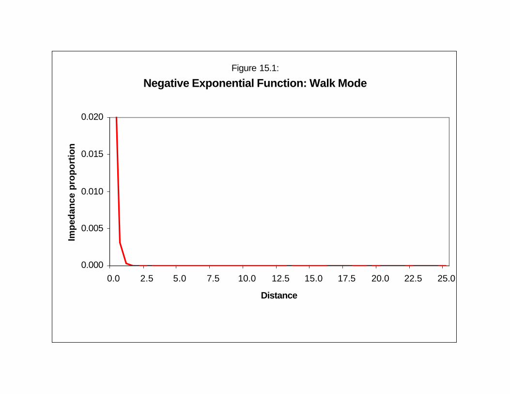
Figure 15.1:

Negative Exponential Function: Walk Mode

0.000

0.005

0.010

0.015

0.020

0.0 2.5 5.0 7.5 10.0 12.5 15.0 17.5 20.0 22.5 25.0

Distance

Imp

edan

ce p

rop

ort

ion

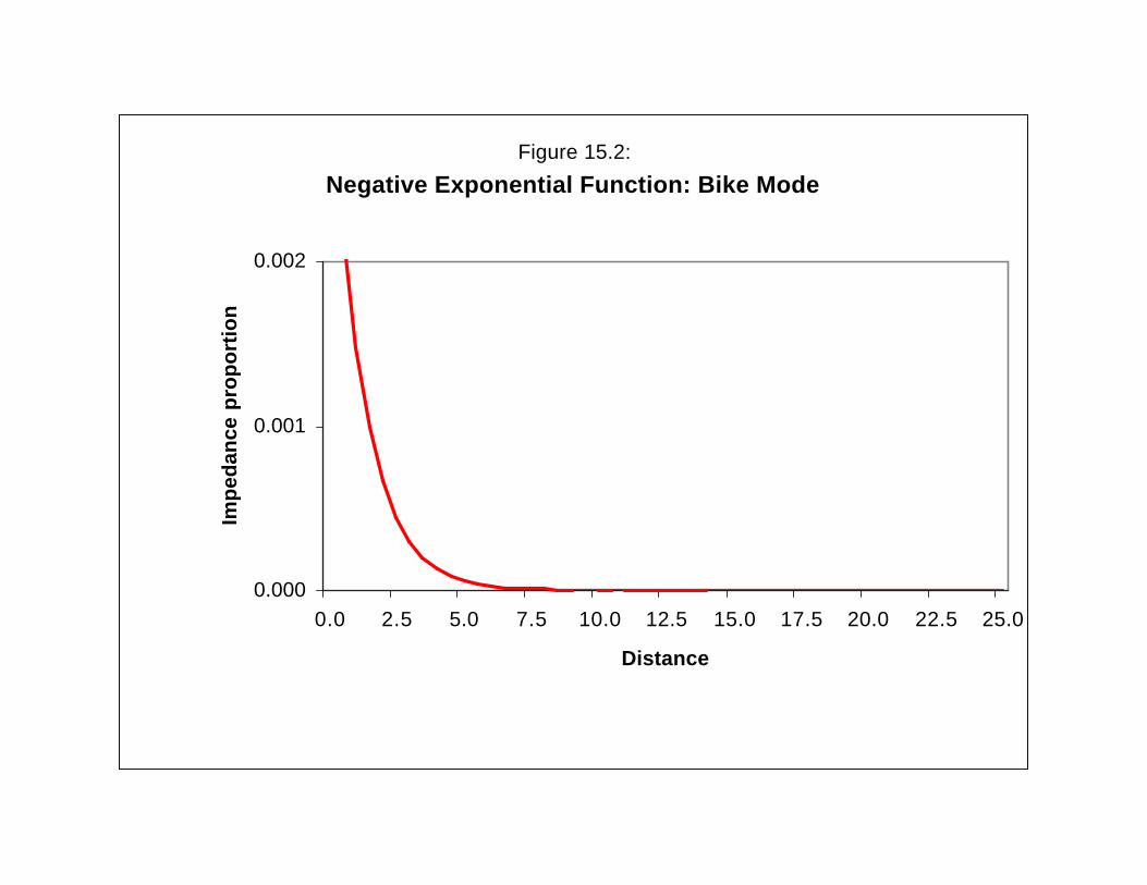
Figure 15.2:

Negative Exponential Function: Bike Mode

0.000

0.001

0.002

0.0 2.5 5.0 7.5 10.0 12.5 15.0 17.5 20.0 22.5 25.0

Distance

Imp

edan

ce p

rop

ort

ion

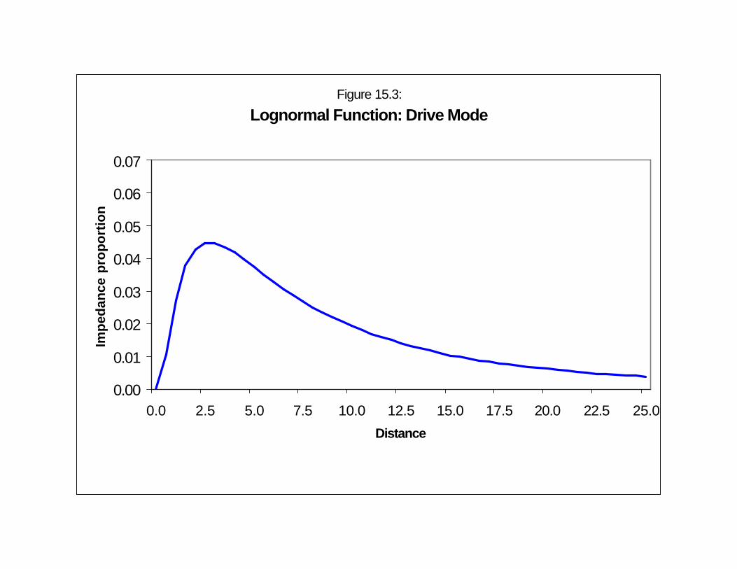
Figure 15.3:

Lognormal Function: Drive Mode

0.00

0.01

0.02

0.03

0.04

0.05

0.06

0.07

0.0 2.5 5.0 7.5 10.0 12.5 15.0 17.5 20.0 22.5 25.0

Distance

Imp

edan

ce p

rop

ort

ion

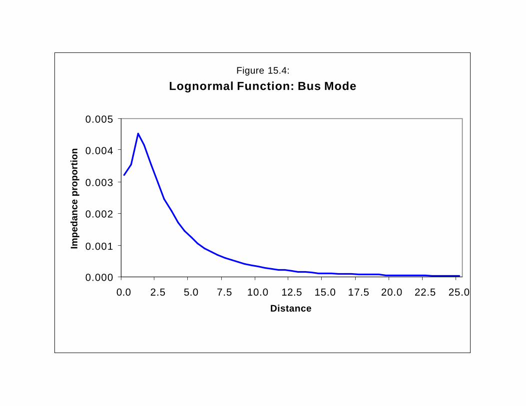
Figure 15.4:

Lognormal Function: Bus Mode

0.000

0.001

0.002

0.003

0.004

0.005

0.0 2.5 5.0 7.5 10.0 12.5 15.0 17.5 20.0 22.5 25.0

Distance

Imp

edan

ce p

rop

ort

ion

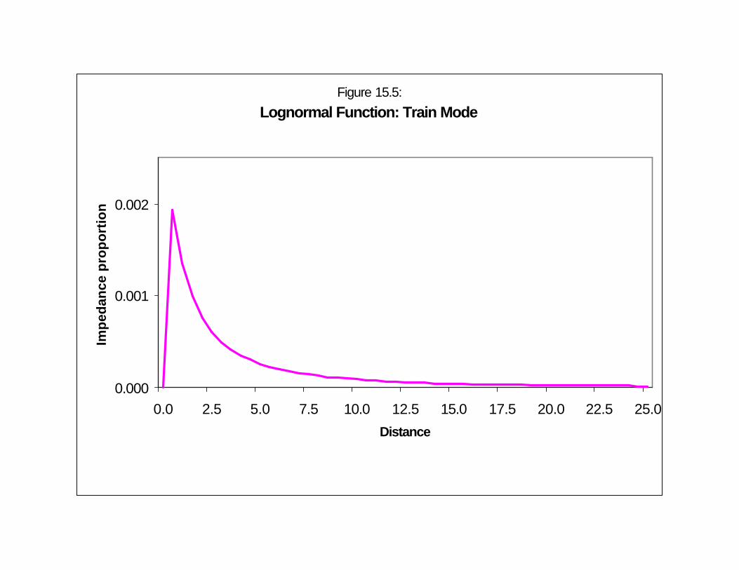
Figure 15.5:

Lognormal Function: Train Mode

0.000

0.001

0.002

0.0 2.5 5.0 7.5 10.0 12.5 15.0 17.5 20.0 22.5 25.0

Distance

Imp

edan

ce p

rop

ort

ion

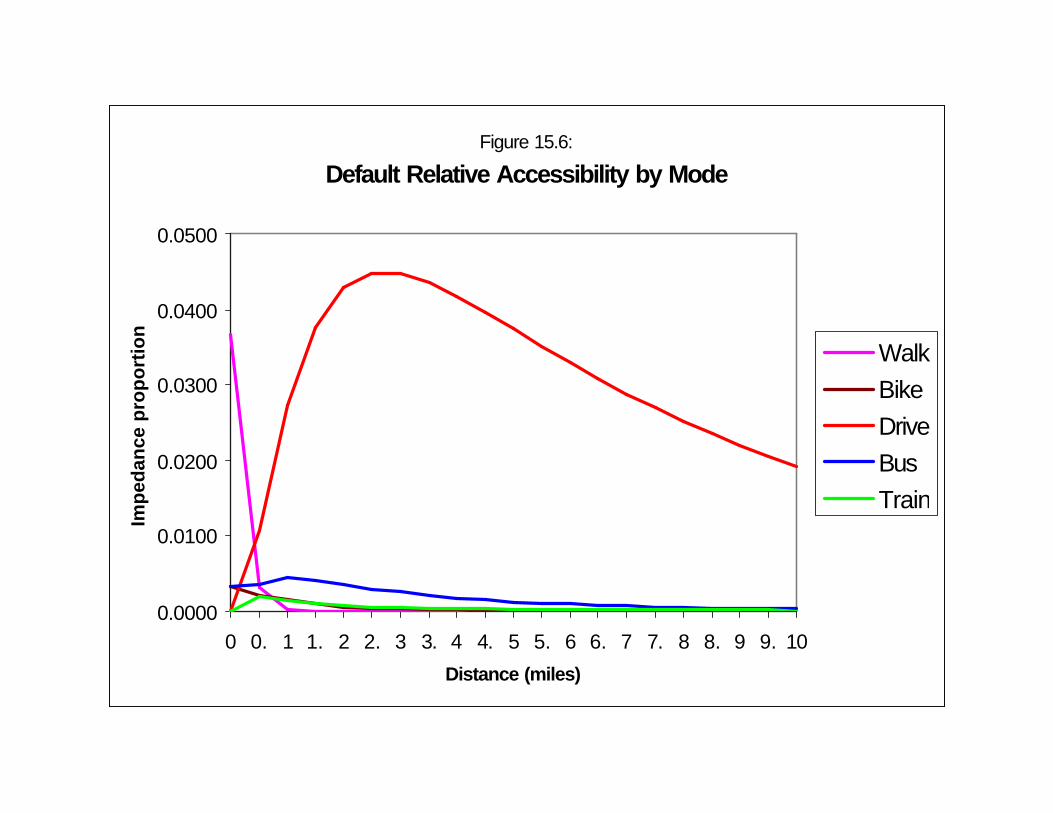
Figure 15.6:

Default Relative Accessibility by Mode

0.0000

0.0100

0.0200

0.0300

0.0400

0.0500

0 0. 1 1. 2 2. 3 3. 4 4. 5 5. 6 6. 7 7. 8 8. 9 9. 10

Distance (miles)

Imp

edan

ce p

rop

ort

ion

WalkBikeDriveBusTrain

15.22

These a ppr oaches wer e discussed in cha pt er 9 (J ourney to Crime) and in chapt er 14(Tr ip Dis t r ibu t ion ). The “Calibra te im pedance funct ion ” rout in e in the Tr ip Dis t r ibu t ionmodule can be used for th is purpose. The adva ntage would be enormous. Instead ofguesses a bout likely impeda nce funct ions of specific t r avel modes, t he user would have afun ction tha t wa s based on rea l da ta . Ther e should be a su bstan t ia l impr ovem en t inmodeling accuracy th a t would resu lt. However, t hese da ta have to be firs t collected.

Cr i m eS t a t III Mode Sp lit Tools

The Crim eS tat mode sp lit m odu le allows t he relat ive accessibility funct ion to becalcu la ted. Figure 15.7 shows t he set up page for the m ode split rout ine a nd figure 15.8shows the setup for modes 1 and 2, in the exa mple “Wa lk ” and “Bicycle”. The setup formodes 3, 4, a nd 5 a re s imila r .

Mo de S pli t S e tu p

On the mode sp lit set up pa ge, the pr edicted origin and pr edicted des t ina t ion filesmust be inpu t as t he pr ima ry an d seconda ry files. If the or igin a nd des t ina t ion files ar eident ica l (i.e., a ll the or igin zones a re included in the dest ina t ion zones), then the file mustbe in pu t as t he pr imary file.

In add it ion , the u ser must inpu t a pr edicted origin -dest ina t ion t r ip file from t he t r ipdist r ibut ion modu le. Fin a lly, an assu med impeda nce value for t r ips from t he “Exter na lzone” mu st be specified. The defau lt is 25 miles. Choose a va lue tha t wou ld rep resen t a‘typica l’ t r ip from outside the study r egion .

For each mode, th e user must pr ovide a label for the name and define themathem at ical function wh ich is to be app lied a nd specify the paramet er s. Th e firs t t imethe rou t ine is opened , th e defau lt va lues a re list ed. However, t he user can change th ese.

Hin t : Once the parameter s a re en tered, t hey ca n be saved on the Opt ion spa ge. Then , th ey can be re-ent ered by loading th e sa ved pa rameters file.

Con stra in Cho ice to N e tw ork

The impeda nce will be ca lcu lat ed either direct ly or is const ra ined to a network. Thedefau lt im pedance is defin ed wit h the type of dis t ance measurement specified on theMea su rem en t Paramet er s page (un der Da ta setup). On the oth er hand, if the impeda nce isto be const ra ined to a n et work, then the n et work has t o be defined.

Defa u l t

The defau lt impedan ce is th at specified on t he Measu rem ent par am eters page. Ifd irect d is t ance is the defau lt d is t ance (on the measurement pa rameters page), then a ll

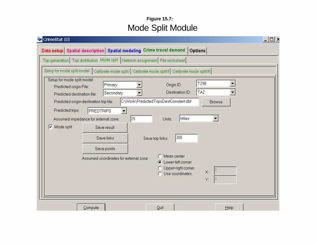
Figure 15.7:

Mode Split Module

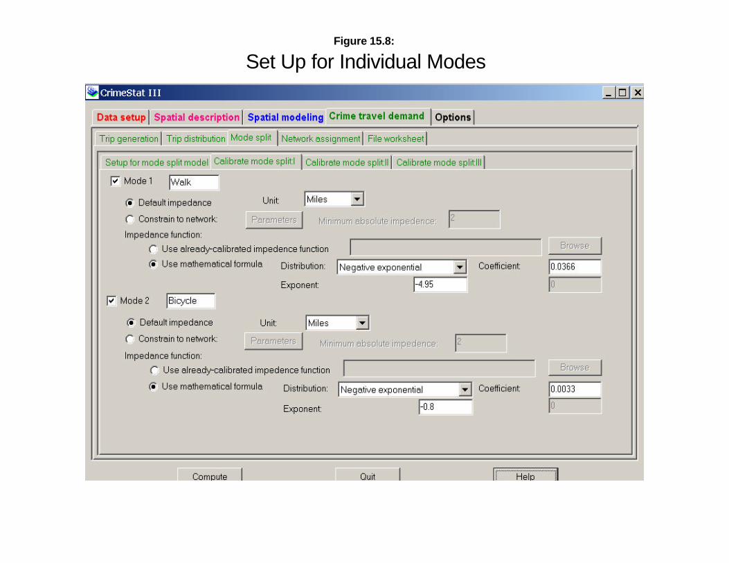
Figure 15.8:

Set Up for Individual Modes

15.25

impeda nces a re calcula ted as a dir ect dis t ance. If indir ect dis t ance is the defau lt , then a llimpeda nces a re calcula ted as in dir ect (Manha t tan) dist ance. If net work dis t ance is thedefau lt, t hen a ll impeda nces a re ca lcu lat ed u sing th e specified net work a nd it s pa rameters;t r avel impedance will a u tomat ica lly be const ra in ed to the network under th is condit ion .

C on st r a i n t o n et w o r k

An impedance ca lcu la t ion shou ld be const r a ined to a network when there a relimit ed choices. F or exa mple, a bus t r ip requir es a bus route; if a par t icu la r zon e is notnea r an exist ing bus r out e, then a dir ect dis t ance ca lcula t ion will be m islea din g sin ce itwill pr obably under est ima te t rue dist ance. Similar ly, for a t r a in t r ip, th ere needs t o be anexist in g t ra in route. Otherwise, t he rout in e will a ssign t ransit t r ips where those a re notpossible (i.e., it will a ss ign t ra in t r ips wh er e t her e a re n o tr a in st a t ions and it will a ss ignbus t r ips wh ere there are no bus rou tes). The r ou t ine does not ‘kn ow’ whether there aret ransit rout es and m ust be t old wher e t hey a re. Even for wa lking, bicycling and dr ivingt r ips , an exist ing net work might pr oduce a m ore r ea list ic t r avel impeda nce th an sim plyassuming a dir ect t r avel pa th .

If the im pedance calcu la t ion is to be const ra in ed to a network, t hen the networkmust be defined . A more exten sive discussion of a network is p rovided in chapt er 3 (underType of dis t ance mea su rem en t on t he Mea su rem en t Paramet er s page) an d in cha pt er 16 inthe discussion of the Tr ip Assignment module. E ssen t ia lly, a network is a ser ies ofconn ected segment s th at specify possible rout es. Ea ch segment h as t wo end nodes (inCrim eS tat, t hey a re ca lled ‘FromNode’ and “ToNode). Dependin g on the type of network,the segmen ts can be bi-dir ectiona l (i.e., t r avel is a llowed in eit her dir ection) or sin gledir ect iona l (i.e., tr avel is a llowed only from t he “FromN ode” to th e “ToNode”).

A cr it ica l component of a network for the mode split rou t ine is tha t t r avel can on lypa ss th rough nodes. This m ea ns t ha t two segm en ts t ha t a re connected can a llow a t r ip t opa ss over t hose two segmen ts wherea s t wo segmen ts t ha t ar e not connected cannot allow at r ip t o pass dir ectly from one t o th e oth er . From out side t he net work, a t r ip connects t o ita t a node. For a t r ansit network, t h is can be cr itical. For a bus rou te, it may or may not beimpor t an t . A p recise bus network defines nodes by bus s tops so tha t a tr ip can ‘en ter ’ or‘leave’ the bus syst em a t a rea l stop. A less pr ecise bus network defines nodes by the endsof segments (e.g., th e end nodes of a TIGER segmen t ). The rou t ine will not know whetherthe node it en ter s or leaves from is a rea l bus s top or not. In the case of bus r out es, itpr obably doesn’t mat ter since they genera lly make very regular st ops (every two or th reeblocks).

Ac cu r a t e ly d e fi n ed t r a n s i t n et w o r k s

For t r a in n etworks , however , it is absolut ely cr itical th a t the network be definedaccura tely. The nodes must be legit imate st a t ions; a t r ip can only en ter or lea ve the t r a insys tem through a st a t ion (i.e ., it cannot en ter or leave a t r a in network a t the en d of anarbit ra ry segm en t node). Most t r avel demand m odels u se very pr ecise bu s a nd t ra innetworks tha t have been car efu lly checked ; where er rors occur , th e networks a re edited

15.26

and u pda ted. If th e u ser does n ot h ave an edited t r ansit net work, one can be m ade in thet r ip a ss ignmen t module. Ther e is a “Cr ea te a t r ansit net work from pr imary file” rout inetha t will d raw segm ents between in put pr im ary file poin t s; the user in put s the st a t ion orbu s s top locat ions a s t he pr imary file and t he r out ine crea tes a net work from one poin t tothe next in the sam e order as in the pr imary file (i.e., the pr imary file needs t o be pr oper lysor ted in order to tr avel). See cha pt er 16 for more in format ion about crea t ing a t r ansitnetwork.

En t er i n g t h e n et w o r k p a r a m e t er s

The network is in put by select in g “Con st ra in to network” and click on the‘Parameter s’ bu t ton . A dia logue is brough t up tha t a llows the user to specify the networkto be used. The network file can be eit her a shape line or polyline file (the defau lt ) oranother file, eith er dBa se IV ‘dbf’, Microsoft Access ‘mdb’, Ascii ‘da t ’, or an ODBC-complia n t file. If th e file is a sh ape file, the r out ine will k now the loca t ions of the n odes . All the user needs t o do is ident ify a weight ing var iable, if used, and possible one wayroutes (‘flags’). For a dBase IV or other file, the X and Y coordina te var iables of the endnodes m ust be defined . These a re ca lled th e “From” node a nd t he “End” node, th ough t hereis n o par t icula r order .

An opt iona l weigh t var iable is a llowed for both a sh ape or dbf file. The r out ineiden t ifies nodes and segmen ts a nd finds the short est pa th . By defau lt , the short est pa th isin terms of dis t ance though each segm ent can be weighted by t ravel t im e, t r avel speed, orgenera lized cost; in th e lat ter case, th e units a re minu tes, hour s, or u nspecified cost u nits.

F in a lly, the number of gr aph segm ents to be ca lcu la ted is defin ed as the networklimit . The defau lt is 50,000 segmen ts. This can be changed, but be su re tha t th is numberis greater than t he number of segments in your network.

Mini m um a bsolu te im p ed a nce

If a mode is const ra ined to a network, an addit iona l const ra int is needed t o ensu rerea listic a lloca t ions of t r ips. This is t he minim um absolu te impeda nce between zones. Thedefau lt is 2 m iles. F or a ny zone pa ir tha t is closer toget her than the m inimum specified (indis tance, tim e in ter val, or cost ), no tr ips will be a llocat ed to th a t mode. Th is const ra in t isto pr event unrea listic t r ips being a ssigned t o int ra -zona l tr ips or t r ips bet ween nearbyzones.

Crim eS tat uses three im pedance com ponents for a const ra in ed network:

1. Th e im peda nce from t he origin zone to th e n ea rest node on the n et work (e.g.,nea res t r a il s t a t ion);

2. Th e im pedance a lon g t he network to the node nearest to the dest in a t ion ; and

3. Th e im peda nce from t ha t node t o th e dest ina t ion zone.

15.27

Since most impeda nce funct ions for a mode const ra ined to a network will ha ve th eh ighest likelihood some d istance from the or igin, it’s possible th a t the mode would beass igned to, essen t ia lly, very sh ort t r ips (e.g., the dist ance from a n origin zone t o a r a ilnetwork a nd t hen back a gain might be modeled a s a h igh likelihood of a t r a in t r ip eventhough su ch a t r ip is ver y un likely).

For ea ch m ode tha t is const ra ined to a n et work, specify the m inimum absolu teimpeda nce. The un its will be th e sa me as t ha t specified by th e measu rement un its . Thedefau lt is 2 miles. If the un it s a re dis t ance, t hen t r ips will on ly be a lloca ted to those zon epairs t ha t a re equal to or great er in dista nce tha n t he minimu m specified. If th e units a ret ravel t ime or speed, t hen t r ips will on ly be alloca ted t o those zone pa irs tha t a re fa r therapar t than the dis t ance t ha t would be t r aveled in tha t t im e a t 30 miles per hour . If theunit s a re cost , t hen the rout in e ca lcu la tes the average cost per mile a lon g t he network andonly a lloca tes t r ips to those zone pa ir s tha t are fa r ther apar t than the d is tance tha t wouldbe t raveled a t tha t aver age cost .

Applying the Relative Access ib i li ty Funct ion

To apply th e relat ive accessibility funct ion , th e pa rameter choices for each mode a reentered int o the mode sp lit r ou t ine. All t r ansit modes a re then const ra inedOnce the mode split setup h as been defined and all tr an sit modes have been const ra ined toa pr oper net work, the m ode split rout ine can be r un .

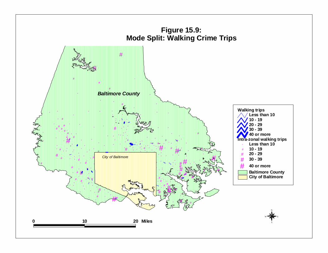
F igure 15.9 shows the top 300 wa lking cr ime t r ips in Ba ltim ore County est ima tedwit h the defau lt accessibility functions. As seen , the vast major ity of walking t r ips a reint ra -zona l (loca l). Ther e are on ly a couple of int er -zona l walk ing t r ip links sh own. Thedefau lt im peda nce funct ion assigned a ppr oximately 4% of the t r ips t o th is mode a nd t heresult is man y int ra -zona l tr ips.

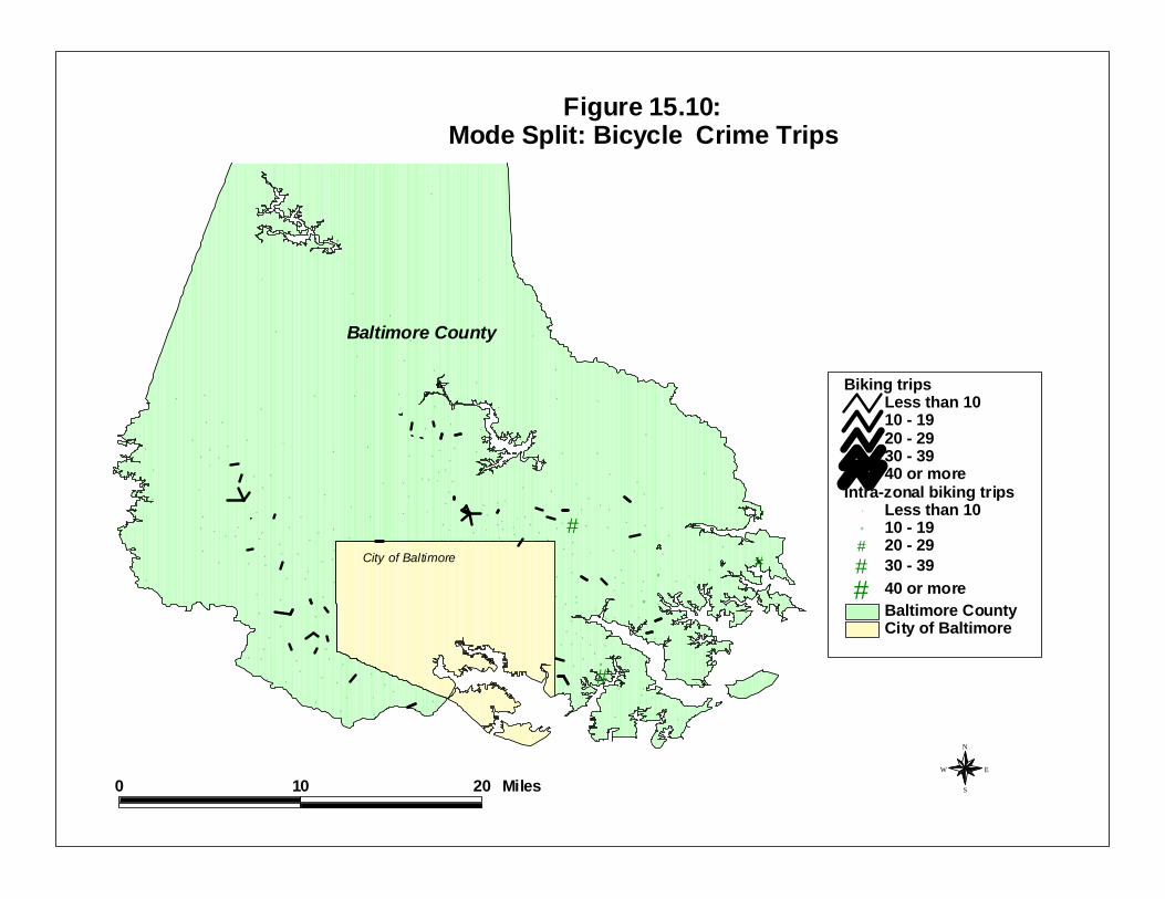
F igure 15.10 sh ows t he top 300 bicycle cr ime t r ips in Ba ltim ore County. Ther e arefewer t r ips by bicycle and they a lso tend to be qu it e loca l. Th e im pedance funct ion used forbicycle tr ips a lloca ted a ppr oximately 1% of a ll t r ips t o th is mode. Thu s, it’s less frequ entthan walking mode. There are pr oport iona tely more int er -zona l tr ips a mong th e top 300than for walk in g t r ips, bu t these tend to be qu it e shor t (t r avel between adjacen t zon es).

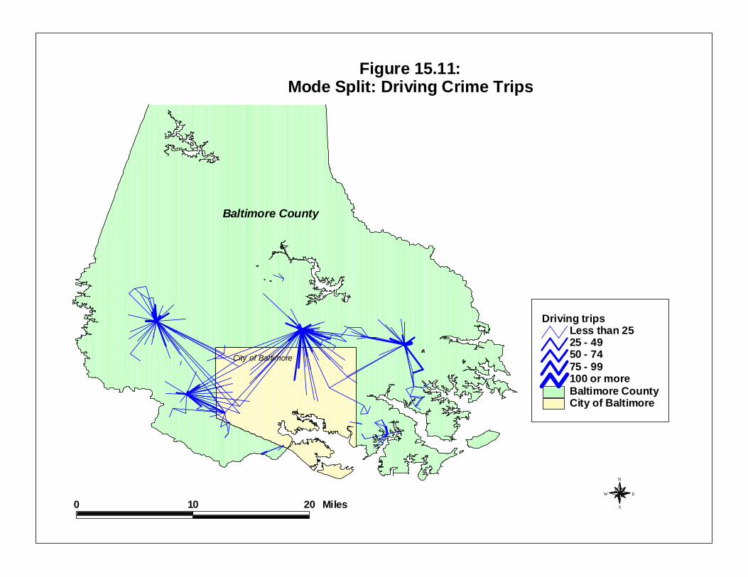
On the oth er hand, dr iving is t he predomin ant t r avel mode for the crim e t r ips(Figu re 15.11). The impeda nce function used a llocat ed approximately 90% of th e t r ips todr iving. The pa t t ern a lmost per fect ly replica tes t he pr edicted t r ip dist r ibut ion (see figur es14.12 and 14.20 in chapt er 14). Fu r ther , th e t r ips a re a lot longer. Among th e top 300links, there were no int ra -zona l dr iving t r ips. The u se of a lognorm al funct ion minim izedin t ra -zona l t r avel.

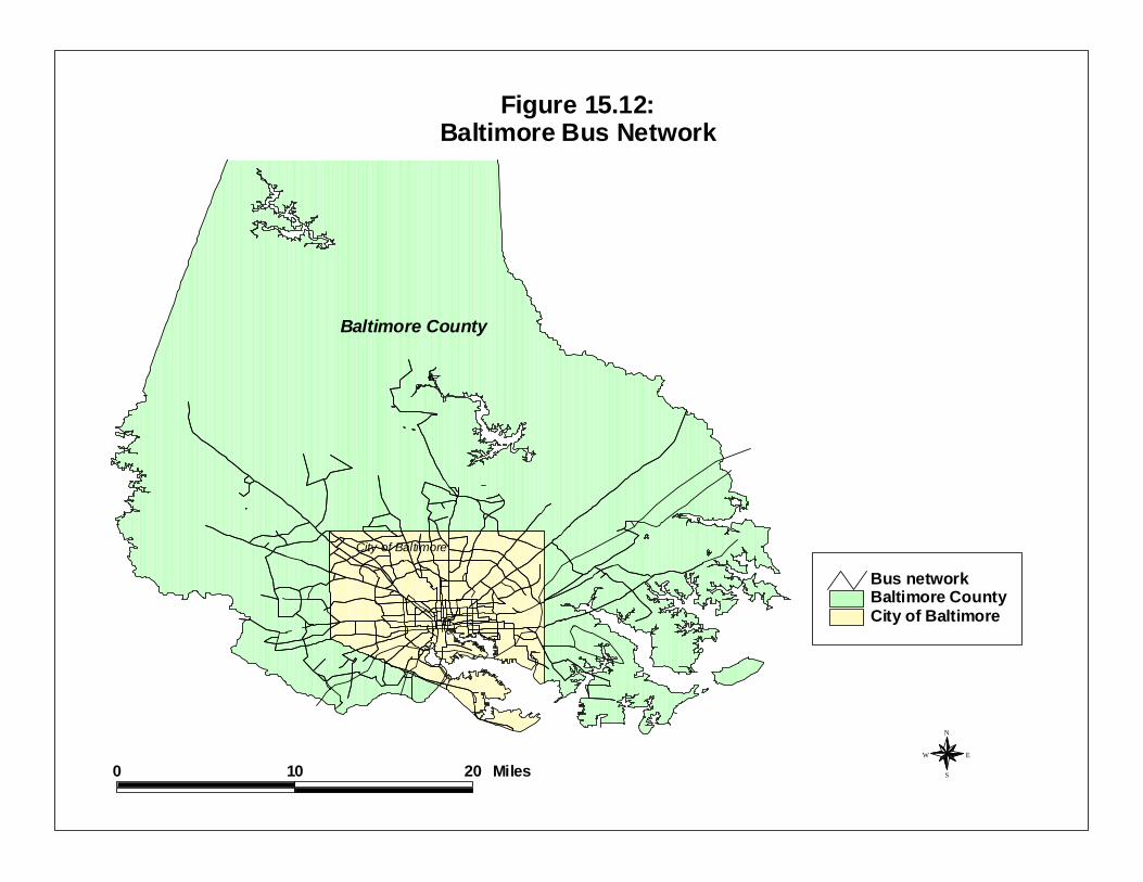
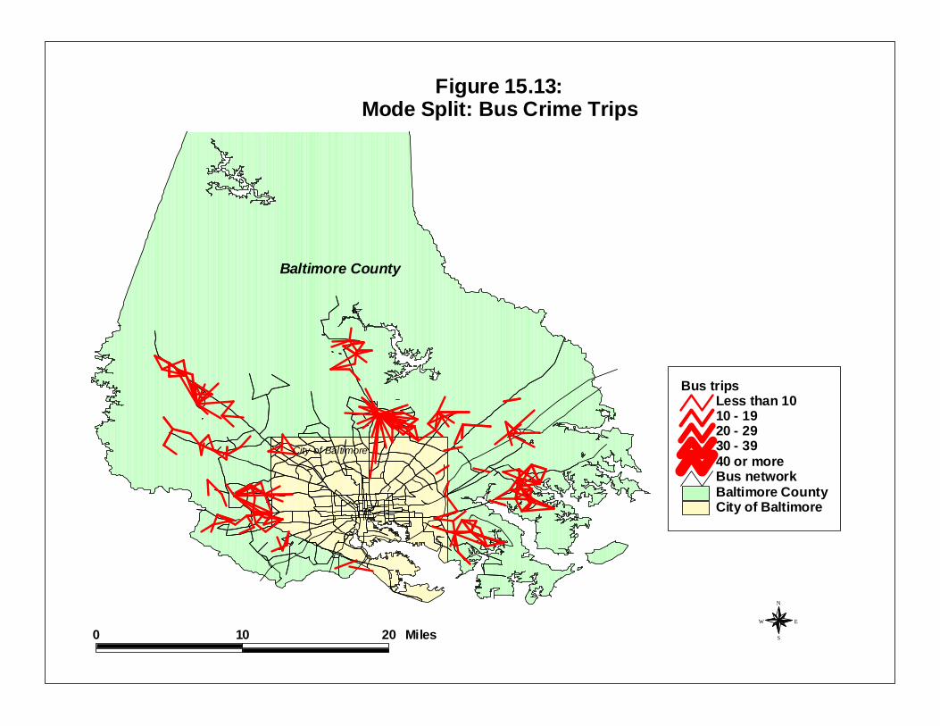
To a lloca te bus and t ra in t r ips, h owever , it was necessary t o const ra in them to anet work. Separa te bu s a nd t ra in net works wer e obta ined from the Ba lt imore Met ropolitanCouncil. F igure 15.12 shows the Ba lt im ore bus network and figure 15.13 shows thepredict ed bus t r ips super im posed over the bus network. Overa ll, a bout 4% of the tota l

#

#

#

#

#

#

##

#

#

#

#

#

#

#

# #

#

#

#

#

#

#

#

#

##

# ##

# #

##

# #

#

#

##

#

#

###

#

##

#

#

#

#

##

#

#

##

#

#

#

#

## #

#

# #

## #

#

## #

#

#

##

#

# #

##

#

#

# #

##

# # #

##

###

##

#

#

#

#

# ##

#

###

#

#

#

#

##

#

#

#

#

###

##

##

##

#

##

#

## #

#

#

##

##

##

#

# ## #

#

#

##

##

#

##

#

##

#

# #

#

#

#

# ##

#

#

##

##

#

### #

#

# #

#

#

##

##

#

##

#

#

## ##

#

#

#

##

#

##

#

## #

#

#

#

#

#

#

#

##

##

##

##

# #

####

#

#

##

##

##

##

#

#

#

#

##

#

#

##

# #

#

##

#

#

#

#

#

##

## #

#

#

#

##

## ## # #

##

#

#

#

## ###

# #

##

#

#

#

#

# #

###

#

##

##

##

#

##

##

#

##

##

#

#

#

#

##

Baltimore County

City of Baltimore

City of BaltimoreBaltimore County

Intra-zonal walking trips# Less than 10# 10 - 19# 20 - 29# 30 - 39

# 40 or more

Walking tripsLess than 1010 - 1920 - 2930 - 3940 or more

Figure 15.9:Mode Split: Walking Crime Trips

N

EW

S0 10 20 Miles

#

#

#

#

#

#

#

#

#

#

#

#

#

#

#

# #

#

#

#

#

#

#

#

#

#

#

# #

#

##

#

#

# #

#

#

#

#

#

#

#

#

#

#

#

#

#

#

#

#

#

#

#

#

##

#

#

#

#

#

# #

#

##

## #

#

#

# #

#

#

#

#

#

# #

#

#

#

#

##

##

##

#

#

#

#

#

#

##

#

#

#

#

###

#

##

#

#

#

#

#

#

#

#

#

#

#

#

##

##

#

#

#

#

#

##

#

###

#

#

##

#

#

#

#

#

##

##

#

#

#

#

##

#

##

#

#

#

#

##

#

#

#

##

#

#

#

##

#

#

#

### #

#

# #

#

#

#

#

##

#

#

#

#

#

#

#

#

#

#

#

#

#

#

#

#

#

#

#

# #

#

#

#

#

#

#

#

##

##

#

#

#

#

# #

##

##

#

#

#

#

##

#

#

#

#

#

#

#

#

#

##

#

#

#

##

#

##

#

#

#

#

#

#

#

#

##

#

#

#

#

#

###

## #

#

#

#

#

#

#

#

#

# #

##

#

#

#

#

#

#

# #

###

#

##

#

#

##

#

#

#

#

#

#

#

#

#

#

#

#

#

#

##

Baltimore County

City of Baltimore

City of BaltimoreBaltimore County

Intra-zonal biking trips# Less than 10# 10 - 19# 20 - 29# 30 - 39

# 40 or more

Biking tripsLess than 1010 - 1920 - 2930 - 3940 or more

Figure 15.10:Mode Split: Bicycle Crime Trips

N

EW

S0 10 20 Miles

Baltimore County

City of Baltimore

City of BaltimoreBaltimore County

Driving tripsLess than 2525 - 4950 - 7475 - 99100 or more

Figure 15.11:Mode Split: Driving Crime Trips

N

EW

S0 10 20 Miles

Baltimore County

City of Baltimore

City of BaltimoreBaltimore CountyBus network

Figure 15.12:Baltimore Bus Network

N

EW

S0 10 20 Miles

Baltimore County

City of Baltimore

City of BaltimoreBaltimore CountyBus network

Bus tripsLess than 1010 - 1920 - 2930 - 3940 or more

Figure 15.13:Mode Split: Bus Crime Trips

N

EW

S0 10 20 Miles

15.33

t r ips wer e a lloca ted t o the bus mode by th e accessibility funct ion . As seen , th e t r ips t end t obe moder a te dist ances a nd t end t o be close t o the bus network. Const ra ining th ese t r ips bythe net work decreases t he likelihood t ha t the r out ine would a ss ign a pa r t icula r t r ip lin ktha t wa s fa r from the bu s work to a bus t r ip.

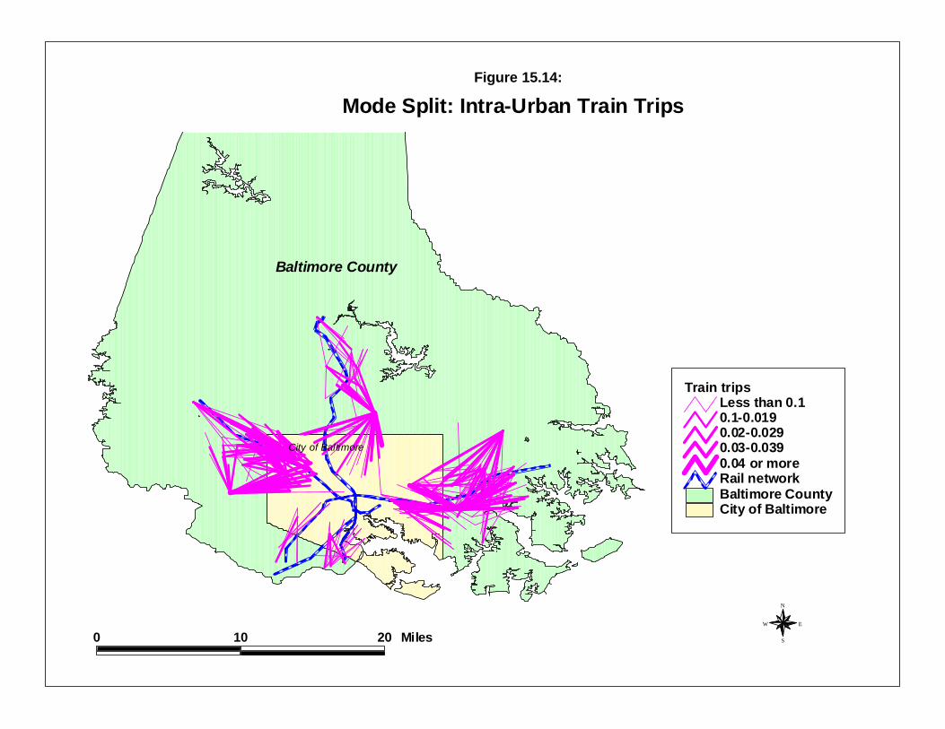
F ina lly, tr a in crime t r ips wer e const ra ined to the t r a in n etwork. F igure 15.14su per imposes t he assigned t ra in t r ips over the int ra -urban ra il network. Overa ll, on ly 1%of the tota l t r ips were a lloca ted to t r a in mode. Therefore, the number of t r ips for any zonepair is quite sma ll. The trips ar e genera lly longer th an th e bus t rips, as m ight be expected,and they a lso tend to fa ll a lon g t he major ra il lines. Some of the t r ips st a r t qu it e fa r fromthe r a il lines, so it ’s possible tha t these a re not r ea list ic r epresen ta t ions. Keep in mindtha t th is is a mathemat ica l m odel a nd is fa r from per fect .

Overa ll, the mode sp lit r ou t ine h as pr odu ced a reasona ble app roximat ion to t r avelmodes for cr im e t r ips. Sin ce there was no da ta upon which to ca libra te the funct ion s,reasona ble guesses were made a bout the accessibility funct ion . The m athemat ica l modelpr oduced a pla usible, though not per fect , represen ta t ion of these a ssumpt ions, gen er a llyfitting int o what we kn ow about crime tr avel pat tern s.

U se fu ln e s s o f Mo de S plit Mo de lin g

The mode split model is a logica l ext ension of the t r avel demand framework. F ort ranspor ta t ion pla nnin g, it is an im por tan t st ep in the process. But , it a lso is im por tan t forcr im e ana lysis . F ir st , it addresses the complexity of t r avel by separa t in g t he t r ips fromspecific or igin s to specific dest in a t ion s in to dis t in ct modes. In th is sense, it adds morerea lism t o our under st anding of cr imin a l tr avel beha vior . The J ourney to Crime lit era ture,which has been used by cr ime a na lyst s a nd crimina l just ice resea rchers t o “under st and”crim ina l t r avel behavior, is sim plis t ic in t h is r espect. I t assumes a sin gle m ode, t houghtha t is ra rely a r t icu lat ed by th e resea rchers. By poin t ing ou t typica l tr avel dist ances byoffenders circum vents t he critical question of how they made th e trip. This was, perha ps,not as crit ica l 50-60 year s a go when most cr imes were committ ed with in a sm allercommunity and it cou ld be assumed tha t mos t offenders wa lked to the cr ime loca t ion . Bu tin post - Wor ld War era , au tomobile t r avel has become increa singly domina te. This m odelassumes tha t the vast major ity of cr ime t r ips a re t aken by au tomobile. While ther e iscur ren t ly no da ta to p rove tha t a sser t ion , it follows from the t ranspor ta t ion pa t t erns tha thave become widespr ead in the U.S. and elsewh ere.

Th er e is a second r ea son wh y an ana lysis of crim e t ravel m ode can be im por tan t . Ifthe limit a t ion s of t r avel m ode in format ion could be im proved th rough bet t er and morecar eful da ta collection by police and other law en forcemen t agencies, th is t ype of an a lysiscould be very u sefu l for policin g. For one th in g, it could a llow more focused policedeployment . F or neighborhoods wit h a predomin ance of walk in g cr im e t r ips, t hen a policefoot pa t rol cou ld be most effect ive. Conversely, for neighborhoods wit h a predomin ance ofdr iving cr ime t r ips , then pa t rol car s a re probably the m ost effective. Police int u it ivelyunderst and t hese cha racter ist ics, but the crim e m ode sp lit model makes th is m ore explicit.

Baltimore County

City of Baltimore

City of BaltimoreBaltimore CountyRail network

Train tripsLess than 0.10.1-0.0190.02-0.0290.03-0.0390.04 or more

Mode Split: Intra-Urban Train Trips

N

EW

S0 10 20 Miles

Figure 15.14:

15.35

For another th in g, a mode split ana lysis of cr im e can bet t er help cr im e prevent ioneffor t s. As the Ba lt imore dat a sugges t , many of t he loca l (in t r a -zona l) cr ime t r ip s a recommit ted a roun d h ous ing pr ojects a nd in very low income communit ies. Most likely, th isis a by product of pover ty, lack of loca l em ploymen t oppor tun it ies , deter iora ted hous ing,and even poor surveilla nce. Sin ce teenagers a re more likely to not own vehicles, it might beexpected tha t the major it y of t hese loca l cr im e t r ips a re commit ted by very youngoffender s . Th is can be usefu l in cr ime p reven t ion . Aga in , t he “Weed and Seed” and a ft er -school progr ams are genera lly t a rgeted to you th from very low in come neighborhoods.What is shown by the m ode sp lit ana lysis is probably the crim e pa t t er ns a ssocia ted wit hthese neighborh oods . Even though it is in tu it ively underst ood, t he m ode sp lit ana lysisquant ifies these r elat ionsh ips in a n explicit m anner .

In sh ort , a mode split ana lysis of crim e t r ips is a n impor tan t tool for crim e a na lyst sand cr im in a l ju st ice researchers. If correct ly ca libra ted, it can help focus policeenforcement and cr im e prevent ion effor t s more specifica lly a nd can im prove the theory ofcr im in a l t r avel behavior .

Hopefully, police depar tmen ts will st a r t to impr ove t he qu a lity of da ta in captur inglikely t r avel modes wh ile t akin g incident report s. Even though m ost police depa r tmentshave an item sim ilar to “Met hod of depa r ture”, ther e has n ot been a lot of em ph asis on t h isin forma t ion and mos t cr ime data set s a r e deficien t on th is in forma t ion . However , withimproved da ta will come more accura te accessibility funct ions a nd, hopefu lly, even rea lu t ility funct ions wh ere actua l cost s a re measu red. The expecta t ion is tha t th is will happenan d we should work towar ds accelerat ing th e process.

Limitations to the Mode Spl i t Methodology

There are a lso limita t ions t o the method, pa r t icu lar ly the aggregat e appr oach . Theaggregat e appr oach does not consider individua ls, on ly proper t ies associat ed with zones(e.g., average t ravel t ime bet ween two zones). As m en t ioned ea r lier , the accessibilityfunct ion used (or the under lying u t ility theory) is much s impler for zones than forindividua ls. Consequ en t ly, th e ana lysis is cruder a t an aggrega te level t han a t anindividua l level. Policy scenar ios a re m uch m ore lim ited wit h aggrega te m ode sp lit thanwith individu a l-level models. For example, if an an a lyst wan ted to explore wha t was thelikely effect of in creased public surveilla nce on walk in g behavior by pick pocket s, it is moredifficult t o do with aggregate dat a t ha n with individua l dat a. For example, it could behypothesized tha t actua l p ick pocket s a re more sensit ive to in creased public surveilla ncethan , say, ca r th ieves, but th is can’t be tes ted a t the aggregat e level. Inst ead, some gener a lcha racter ist ics are a ss igned to all individua ls (e.g., th e number of secur ity per sonnel in azon e).

Second, t he zona l model for mode sp lit (as wit h t r ip d ist r ibu t ion) cannot exp la inin t ra -zon a l t r avel. Th e accessibilit y fu nct ion is applied to in ter -zon a l t r ips; for in t ra -zon a lt r ips, it is in accura te and genera lly defau lt s to sim ple choices (e.g., wa lk in g, bik in g ordr iving). For exam ple, bus or t r a in m ode can rarely be applied at an int ra -zona l levelbecause there a re usua lly too few network segmen t s t ha t t r aver se a zone and the segmen t s

15.36

ra rely stop wit h in the zon e. While th is deficiency a lso applies to the t r ip dis t r ibu t ionmodel, th e depen den ce on a network for t r ansit modes, pa r t icu lar ly, lead t oun derestimat ion of tr an sit use for very short tr ips.

Third , th e zona l mode split m odel cannot explain individua l differences. This goesba ck t o th e first poin t tha t a sin gle u t ilit y fun ction is bein g app lied a t the zona l level. Thus, the value of t ime t o differen t individua ls living in the sa me zone cannot be exam ined;ins tead, everyone is given t he sa me value.

Four th , th e aggregat e mode sp lit m odel does n ot ana lyze time of da y very well. Theproba bilit ies a re assigned to a ll t r ips, r a ther than to t r ips taken a t pa r t icu la r t im es of theda y. To conduct t ha t ana lysis , an ana lyst has t o brea k down crim es by t ime of da y andmodel the differen t per iods sepa ra tely. Aside from being awkward, th e su mmed t r ips n eedto be balanced to ensur e tha t t hey sum t o th e tota l nu mber of tr ips.

F ift h , a nd fin a lly, the mode split model, both aggrega te and disaggrega te, ca nnotexpla in linked trips (somet imes called t rip cha in ing). An offender might leave home oneda y, go ou t to ea t , visit a fr iend , commit a st reet robbery, go to a ‘fence’ to dist r ibut e thegoods, buy dru gs from a dr ug dealer , an d t hen fina lly go home. The mode sp lit m odelt rea t s ea ch of these a s separa te t r ips; in the case of cr ime m ode sp lit, th ere are th reedis t inct cr ime t r ips - comm it t ing the r obber y, selling the s tolen goods to th e ‘fence’, andbuying th e dr ugs from the dr ug dealer . The m odel doesn ’t under st and t ha t these a rerela ted even t s, bu t inst ea d a ss igns separa te m ode pr obabilit ies to each t r ip. Th us, it ispossible to produce absurd choices, such as dr ivin g t o the cr im e scene, t akin g t he bus to thedr ug dea ler , and t hen bik ing home. In th is r espect, t he disa ggrega te approach is equa llyflawed as the aggrega te s ince both t r ea t each t r ip as independen t even t s. The solu t ion toth is lies in a ‘th ird genera tion’ of tr avel modeling in which individua l tr ip ma kers a resim ula ted over a day; activity-based m odeling, as it is k nown, is s t ill in a resea rch s t age(Goulias, 1996; Miller , 1996; Pas, 1996). But , it will even tua lly emer ge as t he domin antt ravel dem and m odelin g a lgorit hm.

Co n clu s io n s

Never theless, m ode sp lit modeling can be a very useful a na lysis st ep for crim eana lysis . It represen t s a new approach for cr im e ana lysis and one wit h many u sefulpossibilities. It will require bu ilding more systemat ic da tabases in order to documentt ravel m odes . Bu t , the possibilit ies tha t it offers u p can be im por tan t for crim e a na lyst sand crimina l just ice resea rchers a like.

In the next cha pt er , th e fina l step in t he cr ime t ravel dem and m odel will bediscussed, net work a ssignment .

15.37

1. There is no reason th is da ta could not be collected. Typica lly, many policedepa r tments collect informat ion on ‘Method of depa r ture’ from a cr ime scene. Whena police r epor t is t aken , t he vict im is somet im es asked how the offen der left thescene. In most cases, t he informat ion is not r ecorded on t he police forms, or a t leas tthose tha t have been exa min ed. This in format ion is probably unreliable in any ca sesin ce m any offenders will t ake the bu s or leave their car nearby while they walk /runto th e crim e scene. St ill, if police depar tmen ts wer e t o put more effort in tocollecting this inform at ion a nd, perh aps, to validat ing it with a rr ested offenders,then it is possible to bu ild up reliable da ta set s tha t can be used to model m odesplit . Unt il then , un for tuna tely, we ha ve to rely on theory ra ther than eviden ce.

2. In a survey of t he t r avel behavior of homeless persons, it was noted tha t mosthomeless walked very sh ort dis t ances over the day even though the va lue of theirt ime wa s very low. For longer t r ips, th ey st ill t ended t o take t he bus ra ther thanwalk. Survey on the t r avel beha vior of very low income individua ls. UrbanPlanning Program, Un iver sit y of Californ ia a t Los Angeles , 1987 (wit h Ma r t inWachs).

3. In test s, I did find t ha t the t wo models p roduced sim ilar pa t t er ns. Th ey wer e off interms of the magnitude of the pr edicted t r ips, but the relat ive pa t t ern was verysim ilar .

4. Houst on-Ga lvest on Area Council. Persona l communica t ion . 2004.

En dn ot e s fo r Ch ap te r 15