8/3/2019 Chapter 20 Structural Reliability Theory
http://slidepdf.com/reader/full/chapter-20-structural-reliability-theory 1/16
Chapter 20
CHAPTER 20
STRUCTURAL RELIABILITY1
P. Thoft-Christensen, Aalborg University
Abstract
In this paper a brief presentation of some of the most fundamental concepts in modern
structural reliability theory is given. The presentation does not claim to be very precise
or exhaustive. The purpose is to show that it is possible to day to evaluate the reliability
of a structural system. A much more satisfactory presentation can be found in the
extensive literature, see e.g. Thoft-Christensen & Baker [1] or Elishakoff [2]. Themethod presented belongs to the so-called level 2 methods, i.e. methods involving
certain approximate iterative calculations to obtain an approximate value of the
probability of failure of the structural system. In these level 2 methods the joint
probability distribution of the relevant variables is often simplified and the failure
domain is idealized in such a way that the reliability calculations can be performed
without an unreasonable amount of work. If the joint probability distribution function
and the true nature of the failure domain are known, then it may, in principle, be
possible to calculate the exact probability of failure. In this case we call the method
used a level 3 method. However, this kind of information is usually not at hand for
ordinary structures. Level 1 methods are methods where the structural and loading
variables are characterized by nominal, values and where the sufficient degree of
reliability is obtained using a number of, for instance, partial coefficients (safety
factors).
1. INTRODUCTION
During the last two decades structural reliability theory has grown from being a pure
research area to a mature research and engineering field. In structural reliability theory
uncertainties in e.g. load intensities and in material properties are treated in a rational
way. Structural engineering used to be dominated by deterministic thinking. In the
1 Proceedings of “Safety and Reliability in Europe”. Pre-Launching Meeting of ESRA, Ispra, Italy,
October 9-12, 1984, pp. 82-99.
251

8/3/2019 Chapter 20 Structural Reliability Theory
http://slidepdf.com/reader/full/chapter-20-structural-reliability-theory 2/16
Chapter 20
deterministic approach design is based on specified minimum material properties and
specified load intensities and a certain procedure for calculating stresses and deflections
is often prescribed in the deterministically based codes. However, it has been
recognized for many decades that for example specifications of minimum material
properties involve a high degree of uncertainty. Likewise, specification of reasonableload intensities is difficult and uncertain. These types of uncertainty combined with
several similar forms of uncertainty result in an uncontrolled risk. It is a fact that total
safety of a structure cannot be achieved even when one is ready to offer a lot of money
on the structure. Further, it is a serious problem with the deterministic approach that no
measure of the safety or reliability of the structure is obtained.
In modern structural reliability theory it is clearly recognized that some risk of
structural failure must be accepted. To obtain some measure of this risk - the
probability of failure - a probabilistic approach seems to be well suitable. By this
approach it is intended to help the structural engineers to design a structure in such a
way that at an acceptable level of probability it will not fail at any time during the
specified design life.
In this paper a brief presentation of some of the most fundamental concepts in
modern structural reliability theory is given. The presentation does not claim to be very
precise or exhaustive. The purpose is to show that it is possible to day to evaluate the
reliability of a structural system. A much more satisfactory presentation can be found in
the extensive literature, see e.g. Thoft-Christensen & Baker [1] or Elishakoff [2]. The
method presented belongs to the so-called level 2 methods, i.e. methods involving
certain approximate iterative calculations to obtain an approximate value of the
probability of failure of the structural system. In these level 2 methods the joint
probability distribution of the relevant variables is often simplified and the failure
domain is idealized in such a way that the reliability calculations can be performedwithout an unreasonable amount of work. If the joint probability distribution function
and the true nature of the failure domain are known, then it may in principle be possible
to calculate the exact probability of failure. In this case we call the method used a level 3 method. However, this kind of information is usually not at hand for ordinary
structures. Level 1 methods are methods where the structural and loading variables are
characterized by nominal values and where the sufficient degree of reliability is
obtained using a number of e.g. partial coefficients (safety factors).
2. BASIC VARIABLES AND FAILURE SURFACES
The reliability analysis presented here is based on the assumption that all relevant
variables can be modeled by random variables (or stochastic processes). These
variables X i, i = 1,…,n called basic variables can be material strengths, external loads
or geometrical quantities. For a given structure the set of variables s x ω ∈ is a
realization of the random vector 1( ,..., )n X X X = . 1( ,..., )n x x x= is a point in an n-
dimensional basic variable space ω .
Next it is assumed that a failure surface (or limit state surface) ( ) 0 f x = divides
the basic variable space ω in a failure region ω f and a safe region ω s. The function
: f Rω → is called the failure function and is defined in such a way that ( ) 0 f x >
when s x ω ∈ , and ( ) 0 f x ≤ when f x ω ∈ . The random variable
M = f ( X ) (1)
252

8/3/2019 Chapter 20 Structural Reliability Theory
http://slidepdf.com/reader/full/chapter-20-structural-reliability-theory 3/16
Chapter 20
is called a safety margin.As an example, consider a single structural element and assume that the load
effect is given by a single load variable S and the strength by a single resistance
variable R. The basic
variables S and R aregiven by their
distribution functions
F S and F R or
alternatively by their
distribution functions
f S and f R, see figure 1.
In this case the safety
margin is M = R - S and the probability of failure is
∫ ∞
∞−
=≤−= dt t f t F S R P P S R f )()()0( (2)
By definition the reliability is
R=1 –P f (3)
In the general case the basic
variables1
( ,..., )n X X X =
are
correlated. However, by a linear
transformation a set of uncorrelated
basic variables 1( , ..., )nY Y Y = can be
obtained. The uncorrelated basicvariable Y is then normalized so that a
set of uncorrelated basic variables
1( ,..., )n Z Z Z = , where the expected
value E[ Z i] and the variance Var[ Z i] =
1, i = 1,..., n, are obtained. By these
transformations the failure surface 1( ) 0 f x = in the x-space is transformed into a failure
surface δω given by ( ) 0 f z = in the corresponding z -space. In the n-dimensional z -
space the so-called reliability index β is defined as the shortest distance from the origin
to the failure surface (see figure 2)
1/ 22
1
minn
i
i
z
z
ω
β =∈∂
= ∑ (4)
In the special cases where the failure surface is linear and all basic variables are
normally distributed it is easy to show that there is a one-to-one relation between the
failure probability P f and reliability index β , namely
)()( 1
f f P P −Φ−=⇔−Φ= β β (5)
where Ф is the standardized normal distribution function. In general, the failure surface
is non-linear, and the basic variables non-normal. The equations (5) are then invalid,
but a so- called generalized reliability index β g can be defined by1( ) g f P β −= −Φ (6)
253
Figure 1. The fundamental case.
Figure 2. Definition of the reliability
index β .

8/3/2019 Chapter 20 Structural Reliability Theory
http://slidepdf.com/reader/full/chapter-20-structural-reliability-theory 4/16
Chapter 20
The estimate of the reliability of a structural system is greatly facilitated if the
basic variables can be assumed normally distributed. The only information needed will
then be the expected values E[ X i] =i X µ , the standard deviations
i X σ and the
coefficients of correlation ji X X ρ between any pair of basic variables X i and X j.However, in general basic variables cannot be modeled with a satisfactory degree of
accuracy by normally distributed variables.
Resistance variables are frequently modeled by the lognormal distribution,
which has the advantage of precluding non-positive values. A number of other
distributions such as the Weibull distribution (type III extreme value distribution) have
the same advantage.
Load variables can in some cases be satisfactorily modeled by normally
distributed variables (permanent loads) but often they are better modeled by an extreme
value distribution, e.g. the Gumbel distribution (type 1 extreme value distribution).
To overcome the problem that basic variables are usually modeled by non-
normal probability distributions a number of different so-called distribution
transformations have been suggested, see e.g. Thoft-Christensen & Baker [1], and
Thoft-Christensen [3]. It is beyond the scope of this paper to discuss these
transformation methods. It will therefore be assumed that all basic variables are
normally distributed.
3. DEFINITIONS OF STRUCTURAL FAILURE
In section 2 a single element and a single failure function (failure mode) are dealt with.
It is of course much more complicated to evaluate the reliability of a real structure,
since failure of a single element does not always imply failure of the complete structuredue to redundancy. In such a case it is useful to consider the structure from a systems
point of view, see e.g. Thoft-Christensen [4]. The following presentation is to some
extent based on reference [4].
Let a structure consist of q failure elements, i.e. elements or points (cross-
sections) where failure can take place, and let the reliability index for failure element i
be β i .An estimate of the structural systems reliability is obtained by taking into account
the possibility of failure of any failure element by modeling the structural system as a
series system with the failure elements as elements. The probability of failure for this
series system is then estimated on the basis of the reliability indices β i , i = 1, 2, . . . , q,
and the correlation between the safety margins for the failure elements. This reliability
analysis is called systems reliability analysis at level 1. In general, it is only necessaryto include some of the failure elements in the series system (namely those with the
smallest β -indices) to get a good estimate of the systems failure probability. The
failure elements included in the reliability analysis are called critical failure elements.The modeling of the system at level 1 is natural for a statically determinate
structure, but failure in a single failure element in a structural system will not always
result in failure of the total system, because the remaining elements may be able to
sustain the external loads due to redistribution of the load effects. This situation is
characteristic of statically indeterminate structures. For such structures systemsreliability analysis at level 2 or higher levels may be reasonable. At level 2 the systems
reliability is estimated on the basis of a series system, where the elements are parallelsystems each with two failure elements - so-called critical pairs of failure elements.
These critical pairs of failure elements are obtained by modifying the structure by
254

8/3/2019 Chapter 20 Structural Reliability Theory
http://slidepdf.com/reader/full/chapter-20-structural-reliability-theory 5/16
Chapter 20
assuming in turn failure in the critical failure elements and adding fictitious load
corresponding to the load-carrying capacity of the elements in failure.
Analyzing modified structures where failure is assumed in critical pairs of
failure elements now continues the procedure sketched above. In this way critical
triples of failure elements are identified and a reliability analysis at level 3 can bemade on the basis of a series system, where the elements are parallel systems each with
three failure elements.
By continuing in the
same way reliability
estimates at level 4, 5,
etc. can be performed,
but in general analysis
beyond level 3 is of
minor interest. System
modeling at levels 1, 2,
and 3 is shown in figure
3.
The behavior of some structures is elastic-plastic. In such cases failure of the
structure is usually defined as formation of a mechanism. The probability of failure of
the structural system is then estimated by modeling the structural system as a series
system with the (significant) mechanisms as elements (see figure 4). Reliability
analysis based on the mechanism failure definition is called systems reliability analysis
at mechanism level.In this
section 3, systemmodeling at a
number of different
levels has been
introduced. The
notation system
level must not be
confused with the
reliability level
treated in section 1.
4. CALCULATION OF FAILURE PROBABILITIES OF FUNDAMENTAL
SYSTEMS
In this section it is shown how approximate failure probabilities for critical failure
elements, series systems and parallel systems can be calculated by linearizing the safety
margins.
First consider a critical failure element with the failure function ( ) f z . It is
assumed that Z is normally distributed, so the probability of failure is
( ( ) 0) ( )
f
f n P P f Z z dz ω
ϕ = ≤ =
∫ (7)
where nϕ is the standardized n-dimensional normal density function.
255
Figure 3. System modeling at levels 1, 2, and 3.
Figure 4. System modeling at mechanism level.

8/3/2019 Chapter 20 Structural Reliability Theory
http://slidepdf.com/reader/full/chapter-20-structural-reliability-theory 6/16
Chapter 20
If the function f is linearised in the so-called design point with distance β to the
origin of the coordinate system, then an approximate value for P f is given by (compare
with (5))
1 1
1 1
( ... 0)
( ... ) ( ) f n n
n n
P P Z Z
P Z Z
α α β
α α β β ≈ + + + ≤= + + ≤ − = Φ −(8)
where 1( ,..., )nα α α = is the directional cosines of the linearised failure surface. β is the
reliability index. Φ is the standardized normal distribution function.
Next consider a series system with k elements. An estimate of the failure
probability s
f p of this series system can be obtained on the basis of linearised safety
margins for the k elements
1 1
1 1
( ( 0)) ( ( ))
1 ( ( )) 1 ( ( ))
1 ( ; )
k k s
f i i i ii i
k k
i i i ii i
k
p P Z P Z
P Z P Z
α β α β
α β α β
β ρ
= =
= =
= + ≤ = ≤ −
= − > − = − − <
= − Φ
U U
U U (9)
where iα and iβ are the directional cosines and the reliability index for failure
element i, i =1, . . . , k and where 1( ,..., )k β β β = . { }
ij ρ ρ = is the correlation
coefficient matrix given byT
ij i j ρ α α = for all ji ≠ . k Φ is the standardized k-
dimensional normal distribution function.
For a parallel system with k elements an estimate of the failure probability p
f p
can be obtained in the following way
1 1
( ( 0)) ( ( )) ( ; )k k
p
f i i i i k i i
p P Z P Z α β α β β ρ = =
= + ≤ = ≤ − = Φ −I I (10)
where the same notation as above is used.
One serious problem in connection with application of (9) and (10) is numerical
calculation of the k-dimensional normal distribution function k Φ or k ≥ 3. However, a
more serious problem is how to identify the failure modes (parallel systems) in figures
3 and 4. The last-mentioned problem is treated in the next sections.
5. IDENTIFICATION OF CRITICAL FAILURE MODES AT LEVELS 1, 2,
AND 3
A number of different methods to identify critical failure modes have been suggested in
the literature. In this paper the β -unzipping method [3] - [8] is used. Only the main
features of the β -unzipping method are presented here. A very detailed description is
given in Thoft-Christensen [3].
At level 1 the systems reliability is defined as the reliability of a series system
with e.g. n elements - the n critical failure elements. Therefore, the first step is to
calculate β -values for all failure elements and then use equation (9). As mentioned
earlier, equation (9) cannot be used directly. However, excellent upper and lower
bounds and good approximations exist. One way of selecting the critical failure
elements is to select the failure elements with β-values in the interval [ β min; β min+ Δβ 1]
256

8/3/2019 Chapter 20 Structural Reliability Theory
http://slidepdf.com/reader/full/chapter-20-structural-reliability-theory 7/16
Chapter 20
where β min is the smallest reliability index and where Δβ 1 is a prescribed positive
number.
At level 2 the systems reliability is estimated as the reliability of a series system
where the elements are parallel systems each with 2 failure elements (see figure 3) - so-
called critical pairs of failure elements. Let the structure be modeled by n failureelements. Let the critical failure element l have the lowest reliability index β of all
critical failure elements. Failure is then assumed in failure element l, and the structure
is modified by removing the corresponding failure element and adding a pair of so-
called fictitious loads F l . If the removed failure element is brittle, then no fictitious
loads are added. However, if the removed failure element l is ductile then the fictitious
load Fl is a stochastic load given by F l = γl Rl where Rl is the load-carrying capacity of
failure element l and where 0 <γl ≤ 1.
The modified structure with the external loads and the fictitious load F l are then
reanalysed and new reliability indices are calculated for all failure elements (except the
one where failure is assumed) and the smallest β-value is called β min. The failure
elements with β-values in the interval [ β min; β min+ Δβ 2] where Δβ 2 is a prescribed positive
number are then in turn combined with failure element l to form a number of parallel
systems. Consider a parallel system with failure elements l and r . During the reliability
analysis at level 1 the safety margin and the reliability index β l for element l were
determined. By the reanalysis of the structure the safety margin and the reliability index
β r , are determined. From these safety margins the correlation coefficient can easily be
calculated. Then it follows from (10) that the probability of failure of this parallel
system is
);,(2 ρ β β r l f P −−Φ= (11)
The same procedure is then in turn used for all critical failure elements and further critical pairs of failure elements are identified. In this way the total series system used
in the reliability analysis at level 2 is determined (see figure 3). The next step is then to
estimate the probability of failure for each critical pair of failure elements (see (11))
and also to determine a safety margin for each critical pair of failure elements. When
this is done generalized reliability indices for all parallel systems in figure 3 and
correlation coefficients between any pair of parallel system are calculated. Finally, the
probability of failure for the series system (figure 3) is estimated. The so-called
equivalent linear safety margin introduced by Gollwitzer & Rackwitz [9] is used as
approximations for safety margins for the parallel systems.
The method presented above can easily be generalized to higher levels N> 2. At
level 3 the estimate of the systems reliability is based on so-called critical triples of failure elements, i.e. a set of three failure elements. The critical triples of failure
elements are identified by the β-unzipping method and each triple forms a parallel
system with three failure elements. These parallel systems are then elements in a series
system (see figure 3). Finally, the estimate of the reliability of the structural system at
level 3 is defined as the reliability of this series system.
Assume that the critical pair of failure elements (l,m) has the lowest reliability
index β l,m of all critical pairs of failure elements. Failure is then assumed in the failure
elements l and m, and the structure is modified by adding for each of them a pair of
fictitious loads F l and F m. The modified structure with the external loads and the
fictitious loads F l and F m is then reanalysed and new reliability indices are calculated
for all failure elements (except l and m) and the smallest β-value is called β min. Failureelements with β-values in the interval [ β min; β min+ Δβ 3], where Δβ 3 is a prescribed positive
257

8/3/2019 Chapter 20 Structural Reliability Theory
http://slidepdf.com/reader/full/chapter-20-structural-reliability-theory 8/16
Chapter 20
number, are then in turn combined with failure elements l and m to form a number of
parallel systems.
The next step is then to evaluate the failure probability for each of the critical
triple of failure elements. Consider the parallel system with failure elements l, m, and r .
During the reliability analysis at level 1 the safety margin for failure element l isdetermined and during the reliability analysis at level 2 the safety margin for the failure
element m is determined. The safety margin for safety element r is determined during
the reanalysis of the structure. From these safety margins the reliability indices β l , β m,
and β r and the correlation matrix ρ can easily be calculated. The probability of failure
for the parallel system then is
3 ( , , ; ) f l m r P β β β ρ = Φ (12)
6. IDENTIFICATION OF CRITICAL FAILURE MODES AT MECHANISMLEVEL
When failure of a structure is defined as formation of a mechanism the β-unzipping
method is used in connection with fundamental mechanisms. Consider an elasto-plastic
structure and let the number of potential failure elements (e.g. yield hinges) be n. It is
then known from the theory of plasticity that the number of fundamental mechanisms is
m = n - r , where r is the degree of redundancy. All other mechanisms can then be
formed by linear combinations of the fundamental mechanisms.
The total number of mechanisms for a structure is usually too high to include all
possible mechanisms in the estimate of the systems reliability. It is also unnecessary to
include all mechanisms because the majority of them will in general have a relatively
small probability of occurrence. Only the most critical or most significant failure modesshould be included. The problem is then how the most significant mechanisms (failure
modes) can be identified. In this section it is shown how the β-unzipping method can be
used for this purpose. It is not possible to prove that the β-unzipping method identifies
all significant mechanisms, but experience with structures where all mechanisms can be
taken into account seems to confirm that the β-unzipping method gives reasonably
good results. Note that since some mechanisms are excluded the estimate of the
probability of failure by the β-unzipping method is a lower bound for the probability of
failure.
The first step is to identify all fundamental mechanisms and calculate the
corresponding reliability indices. The next step is then to select a number of
fundamental mechanisms as starting points for the unzipping. By the β-unzippingmethod this is done on the basis of the reliability index β min for the real fundamental
mechanism that has the smallest reliability index and on the basis of a preselected
constant ε1 (e.g. ε1 = 0.50). Only real fundamental mechanisms with β-indices in the
interval [ β min; β min + ε1] are used as starting mechanisms in the β-unzipping method. Let
f β β β ≤≤≤ ...21 be an ordered set of reliability indices for f real fundamental
mechanisms 1,2,…, f , selected by this simple procedure.
The f fundamental mechanisms selected as described above are now in turn
combined linearly with all m (real and joint) mechanisms to form new mechanisms.
First the fundamental mechanism 1 is combined with the fundamental mechanisms 2, 3,
. . . , m and reliability indices m,12,1 ,..., β β for the new mechanisms are calculated. Thesmallest reliability index is determined, and the new mechanisms with reliability
258

8/3/2019 Chapter 20 Structural Reliability Theory
http://slidepdf.com/reader/full/chapter-20-structural-reliability-theory 9/16
Chapter 20
indices within a distance ε2 from the smallest reliability index are selected for further
investigation. The same procedure is then used on the basis of the fundamentalmechanisms 2, …,f and a failure tree as the one shown in figure 5 is constructed.
More mechanisms can be identified on the basis of the combined mechanisms
in the second row of the failure tree in figure 5 by adding or subtracting fundamental
mechanisms. By repeating this simple procedure the failure tree for the structure in
question can be constructed. 'The maximum number of rows in the failure tree must be
chosen and can typically be m + 2, where m is the number of fundamental mechanisms.
A satisfactory estimate of the systems reliability index can usually be obtained by using
the same ε2-value for all rows in the failure tree.
The final step in the application of the β-unzipping method in evaluating the
reliability of an elasto-plastic structure at mechanism level is to select the significant
mechanisms from the mechanisms identified in the failure tree. This selection can, inaccordance with the selection criteria used in making the failure tree, e.g. be made first,
identifying the smallest β -value, β min of all mechanisms in the failure tree and then
selecting a constant ε3 . The significant mechanisms are then by definition those with ε-
values in the interval [ β min; β min + ε3]. The probability of failure of the structure is then
estimated by modeling the structural system as a series system with the significant
mechanisms as elements (see figure 4).
The systems reliability index β S is by definition equal to the generalized
reliability index, i.e.
)(1
f S P −Φ−=β (13)
where P f is the probability of failure of the (structural) system.
7. EXAMPLE
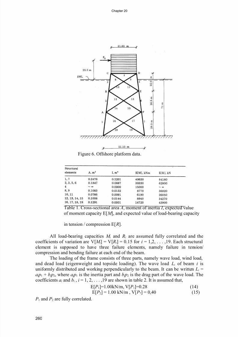
Consider the plane frame shown in figure 6. It is part of an offshore platform. It has 19
structural elements which are all tubular beam elements made of steel with the modulus
of elasticity E = 0.21×10⁹ kN/m2. The cross-sectional areas Ai, moment of inertia I i,expected value of moment capacity E[M i] and expected value of load-bearing capacity
in tension/compression E [ Ri], i = 1,2, . . . , 19 are shown in table 1.
259
Figure 5. Construction of new mechanisms.
8/3/2019 Chapter 20 Structural Reliability Theory
http://slidepdf.com/reader/full/chapter-20-structural-reliability-theory 10/16
Chapter 20
All load-bearing capacities M i and Ri are assumed fully correlated and thecoefficients of variation are V[M i] = V[ Ri] = 0.15 for i = 1,2, . . . ,19. Each structural
element is supposed to have three failure elements, namely failure in tension/
compression and bending failure at each end of the beam.
The loading of the frame consists of three parts, namely wave load, wind load,
and dead load (eigenweight and topside loading). The wave load Li of beam i is
uniformly distributed and working perpendicularly to the beam. It can be written Li =
ai p1 + bi p2, where a j p1 is the inertia part and bi p2 is the drag part of the wave load. The
coefficients ai and bi , i = 1, 2, . . . ,19 are shown in table 2. It is assumed that,
E[ P 1]=1.00kN/m, V[ P 1]=0.28 (14)
E[ P 2] = 1.00 kN/m , V[ P 2] = 0,40 (15)
P 1 and P 2 are fully correlated.
260
Figure 6. Offshore platform data.
Table 1. Cross-sectional area A, moment of inertia I , expected value
of moment capacity E[M ], and expected value of load-bearing capacity
in tension / compression E[ R].

8/3/2019 Chapter 20 Structural Reliability Theory
http://slidepdf.com/reader/full/chapter-20-structural-reliability-theory 11/16
Chapter 20
At the intersection point A, B, C, D, E, F
(see figure 6) the wave load consists of a
horizontal part H i (positive to the right) and
a vertical part V i (positive downwards), i = A,. . , . , F. H i and V i can be written
H i = ci P l + d i P 2 (16)
V i = ei P l + f i P 2 (17)
where ci P l and ei P l are the inertia parts and
d i P 2 and f i P 2 are the drag parts of the loading.
The coefficients ci, d i, ei and f i, i = A, … , F
are shown in table 3. It is assumed that
E[ P l] = 1.00 kN , V[ P l] = 0.28 (18)
E[ P 2] = 1.00 kN , V[ P 2] = 0.40 (19)
At the left hand side of the topside the lowest 6.0 m are loaded by the load
29.831 P 2 is the load at the lowest 6.0 m. The lowest 4.3 m of the right hand side is
loaded by the load 11.175 P 1 + 22.267 P 2, where P 1 and P 2 are defined earlier. The wind
load P 3 is shown in figure 6. E[ P 3] = 1000 kN and V[ P 3] = 0.4. The dead load is two
vertical single loads P 4 at the intersection points C and D (positive downwards) withE[ P 4] = 30377 kN and V[ P 4] = 0.05. It is assumed that P 1, P 2, P 3 are fully correlated
and that P 4 is uncorrelated with P 1, P 2, P 3.As mentioned earlier, each structural element has 3 failure elements so that the
total number of failure elements for this structure is 3 × 19 = 57. The first step in the
reliability analysis is calculation of reliability indices βi, i = 1, … , 57 for all failure
elements. It turns out that failure element 53 (see figure 7) in structural element 6 has
the lowest β-index, namely β53 = 2.93. With Δβ1 = 2.0, 8 critical failure elements are
identified. They are indicated in figure 7, and their β-indices are given in table 4.
261
Table 2. Loading coefficients.
Table 3. Loading parameters.

8/3/2019 Chapter 20 Structural Reliability Theory
http://slidepdf.com/reader/full/chapter-20-structural-reliability-theory 12/16
Chapter 20
The critical failure elements given in table 4
supplemented with the correlation coefficients
between the corresponding safety margins are used in
estimating the systems reliability at level 1. It turns out
that some of the safety margins are almost fully
correlated ( ρ > 0.98) so that the number of critical
failure elements can be reduced when estimating the
failure probability of the system at level 1. Only 4
critical failure elements (nos. 53, 5, 9, 55) have mutual
correlation coefficients smaller than or equal to 0.98.
The correlation matrix (between the safety
margin in the same order) is
The so-called Ditlevsen bounds for the systems probability of failure at level 1
(see figure 8) are identical and equal to
001696.01 = f P (20)
The corresponding systems reliability index at level 1 is
93.21 =S β (21)
Figure 8. Series system used in estimating the systems reliability at level 1.
262
Figure 7. Critical failure
elements. X = failure in
bending. I = failure in
compression.
Table 4. Critical failure elements. c = failure in compression.
b = failure in bending.

8/3/2019 Chapter 20 Structural Reliability Theory
http://slidepdf.com/reader/full/chapter-20-structural-reliability-theory 13/16
Chapter 20
At level 2 it is initially assumed that the ductile failure element 53 fails
(compression failure in structural element 6). The modified structure is then analyzed
and new reliability indices are calculated for all the remaining failure elements. With
2β ∆ = 0.25 a number of critical pairs of failure elements are identified. This procedure
is then performed with all critical failure elements. It turns out that 22 critical pairs of failure elements are identified but only seven of them are not fully correlated ( ρ ≤0.98). The seven critical pairs of failure elements are shown in figure 9 with
generalized β -indices for the parallel systems based on approximate equivalent safety
margins.
Figure 9. Series system used in estimating the systems reliability at level 2.
The correlation matrix is
The three most significant failure modes at level 2 are shown in figure 10. It
follows from the correlation matrix that they are highly correlated. It is therefore to be
expected that the systems reliability index2
S β at level 2 is equal to the reliability index
for the most serious failure mode. The Ditlevsen bounds for the generalized reliability
index are identical and equal to
2S β = 3.12 (22)
Figure 10. The three most significant failure modes at level 2.
263

8/3/2019 Chapter 20 Structural Reliability Theory
http://slidepdf.com/reader/full/chapter-20-structural-reliability-theory 14/16
Chapter 20
At level 3 (with 3β ∆ = 0.1) six not fully correlated triples of failure elements are
identified (see figure 11).
Figure 11. Series system used in estimating the systems reliability at level 3.
The correlation matrix is
It follows from the correlation matrixthat the most significant failure mode at level 3
(see figure 12) is almost fully correlated ( ρ =0.98) with the remaining failure modes. It can
therefore be expected that the systems reliability
index at level 33
S β is equal to the reliability index
β = 3.16 for the failure mode with the failure
elements 53, 56, and 40. This expectation is
confirmed by calculation of the Ditlevsen bounds.
Therefore,
3S β = 3.16 (23)
It is of interest to note that the estimates of the
systems reliability index at levels 1 and 2 are very
different, but that only a small increase takes place
from level 2 to level 3 (see table 5). This is due to the fact that after failure in two
structural elements the remaining structural elements can only sustain a small increase
in the loading. It is therefore to be expected that an estimate of systems reliability
indices at higher levels than level 3 will only result in slightly higher β -values than
3.16.
264
Figure 12. The most
significant failure mode at
level 3. I = failure incompression. = failure in
bending.

8/3/2019 Chapter 20 Structural Reliability Theory
http://slidepdf.com/reader/full/chapter-20-structural-reliability-theory 15/16
Chapter 20
Table 5. Comparison of systems reliability indices at different levels.
The numerical calculations in this example are made in cooperation with J. D. Sørensen
and G. Sigurdsson. A CDC-Cyber 170-730 Computer was used for this purpose.
8. CONCLUSIONS
In this paper an engineering area is presented where modern structural reliability theory
has been used with some success, namely static loading of elasto-plastic framed and
trussed structures. The so-called β-unzipping method to identify significant failure
modes is used, but several other methods exist. Brittle behavior and stability problems
can also be treated by this method. Recent research results seem to indicate that this
method is convenient in optimum design, where the constraints are reliability
conditions. However, it is not yet clear how to include dynamic behavior and fatigue
problems. The systems reliability index calculated for a given structure has to be
considered a relative measure of the reliability of the structure and not an absolutemeasure.
Modem structural reliability theory has been used with success in many other
important areas such as dynamic response analysis, quality control, gross errors,
hydrodynamics, code theory, soil mechanics, dams, concrete structures, offshore
engineering, fatigue, ship design, etc. More details concerning these and many more
areas can be found in the vast literature, see e.g. references [1], [2], [10], [11], and [12],
and also a recently published bibliography [13] containing approximately 1500
references.
9. REFERENCES
[1] Thoft-Christensen, P. & Baker, M. J.: Structural Reliability Theory and its Applications. Springer-Verlag, Berlin - Heidelberg - New York, 1982.
[2] Elishakoff, I.: Probabilistic Methods in the Theory of Structures. John Wiley &
Sons, New York - Chichester - Brisbane - Toronto - Singapore, 1983.
[3] Thoft-Christensen, P.: Reliability Analysis of Structural Systems by the β-
Unzipping Method. Institute of Building Technology and Structural Engineering,
Aalborg University Centre, Aalborg, Report 8401, March 1984.
[4] Thoft-Christensen, P. & S0rensen, J. D.: Optimization and Reliability of Structural
Systems. Presented at the NATO Advanced Study Institute on Computational
Mathematical Programming, Bad Windsheim, FRD, July 1984. Institute of Building Technology and Structural Engineering, Aalborg University Centre,
Aalborg, Report 8404, July 1984.
[5] Thoft-Christensen, P.: The β-Unzipping Method. Institute of Building Technology
and Structural Engineering, Aalborg University Centre, Aalborg, Report
8207,1982 (not published).
[6] Thoft-Christensen, P. & Sørensen, J. D.: Calculation of Failure Probabilities of Ductile Structures by the β-Unzipping Method. Institute of Building Technology
and Structural Engineering, Aalborg University Centre, Aalborg, Report 8208,
1982.
[7] Thoft-Christensen, P. & Sørensen, J. D.: Reliability Analysis of Elasto-Plastic
Structures. Proc. 11. IFIP Conf. »System Modelling and Optimization»,Copenhagen, July 1983. Springer-Verlag, 1984, pp. 556-566.
265

8/3/2019 Chapter 20 Structural Reliability Theory
http://slidepdf.com/reader/full/chapter-20-structural-reliability-theory 16/16
Chapter 20
[8] Thoft-Christensen, P.: Reliability of Structural Systems. Advanced Seminar on
Structural Reliability, Ispra, Italy, June 1984. Proceedings to be published by D.
Reidel Publ. Co., Dordrecht, The Netherlands, 1985.
[9] Gollwitzer, S. & Rackwitz, R.: Equivalent Components in First-order System
Reliability. Reliability Engineering, Vol. 5, 1983, pp. 99-115.[10] Augusti, G., Baratte, A. & Casciati, F.: Probabilistic Methods in Structural
Engineering. Chapman & Hall, London - New York, 1984.
[11] Thoft-Christensen, P. (ed.): Reliability Theory and Its Application in Soil
Mechanics. Proc. NATO ASI, Bornholm, Denmark, 1982. Martinus Nijhoff
Publishers, The Hague - Boston - Lancaster, 1983.
[12] Ang, A. H.-S. & Tang, W. H.: Probability Concepts in Engineering, sign. Vol. II
Decision, Risk and Reliability. John Wiley & Sons, Chichester - Brisbane -
Toronto - Singapore, 1984.
[13] Thoft-Christensen, P. & Sørensen, J. D.: A Bibliographical Survey of Structural
Reliability. Structural Reliability Theory, paper no. 7. Institute of Building
Technology and Structural Engineering, Aalborg University Centre, Aalborg,
Report 8408, September 1984.
266
Recommended