Choice of Variables in Vector Autoregressions∗
Marek Jarocinski
European Central Bank
Bartosz Mackowiak
European Central Bank and CEPR
September 2011
Abstract
Suppose that a dataset with N time series is available. N1 < N of those are the
variables of interest. You want to estimate a vector autoregression (VAR) with the
variables of interest. Which of the remaining N−N1 variables, if any, should you include
in the VAR with the variables of interest? We develop a Bayesian methodology to answer
this question. This question arises in most applications of VARs, whether in forecasting
or impulse response analysis. We apply the methodology to the euro area data and
find that when the variables of interest are the price level, GDP, and the short-term
interest rate, the VAR with these variables should also include the unemployment rate,
the spread between corporate bonds and government bonds, the purchasing managers
index, and the federal funds rate. Of independent interest, we develop Bayesian tests
of block-exogeneity – Granger causality – in VARs.
Keywords: Bayesian vector autoregression, Bayesian model choice, block-exogeneity,
Granger causality. (JEL: C32, C52, C53.)
∗Jarocinski: European Central Bank, Kaiserstrasse 29, 60311 Frankfurt am Main, Germany (e-mail:
[email protected]); Mackowiak: European Central Bank, Kaiserstrasse 29, 60311 Frankfurt am Main,
Germany (e-mail: [email protected]). We thank for helpful comments Gianni Amisano, John
Geweke, David Madigan, Tao Zha and especially Chris Sims. We also thank seminar participants at the
National Bank of Poland and Humboldt University Berlin. The views expressed in this paper are solely
those of the authors and do not necessarily reflect the views of the European Central Bank.
1 Introduction
Vector autoregressions (VARs) are a standard tool for forecasting and impulse response
analysis. When we set out to estimate a VAR, we rarely know a priori which variables to
include in the VAR. Typically, we have a small number of variables we are interested in and
we know that, in principle, we can include many other variables in the VAR. For example,
when we want to forecast inflation and GDP, we realize that many variables may improve
our forecast. To take another example, when we want to estimate the impulse response
of hours worked to a technology shock, we realize that the inclusion or exclusion of many
“control variables” may affect our estimate. Often, we include or exclude one variable at a
time and evaluate informally whether “the results change”.
This paper studies formally the choice of variables in VARs. We study the following
question. Suppose that a dataset with N time series is available. N1 < N of these time
series are the variables of interest. Let all other N −N1 time series be called the remaining
variables. We want to estimate a VAR with the variables of interest. Which of the remaining
variables, if any, should we include in the VAR with the variables of interest?
We develop a methodology to answer this question. The idea behind this methodology
is as follows. Let y be the vector of all variables in the dataset. Consider a partition of y into
two subvectors, y = yi, yj, such that all variables of interest are elements of yi. Note that
yi includes all variables of interest and possibly some remaining variables and yj includes the
other remaining variables. Suppose that yi is block-exogenous to yj . The statement “yi is
block-exogenous to yj” means that “the elements of yj are of no help in improving a forecast
of any variable contained in yi based on lagged values of all the elements of yi alone”.1 If
yi is block-exogenous to yj , one can exclude yj from a VAR model with yi. In other words,
only those remaining variables that are elements of yi are helpful in modeling the variables
of interest. This reasoning leads to the following conclusion. The decision about which
variables to include in a VAR with variables of interest involves evaluating block-exogeneity
restrictions in a VAR with all variables. The block-exogeneity restrictions have the form:
1The statement “yi is block-exogenous to yj” is the same as the statement that “the variables in yj do
not Granger-cause any of the variables in yi”. See Section 2.1. Throughout this paper we use the term
“block-exogeneity”, but we could have also used the term “Granger causality”.
1

“the variables of interest and a subset of the remaining variables are block-exogenous to
every other variable”.
We develop the Bayesian implementation of this methodology. We work with Bayesian
VARs, because Bayesian VARs are popular and we find Bayesian inference appealing. To
evaluate a block-exogeneity restriction in a VAR, a Bayesian compares the marginal like-
lihood of the data implied by that VAR without restrictions with the marginal likelihood
of the data implied by that VAR given the block-exogeneity restriction. It is well known
that, with conjugate priors, the marginal likelihood implied by an unrestricted VAR can
be evaluated analytically. We show how to evaluate conveniently the marginal likelihood
implied by a VAR with one block-exogeneity restriction and multiple block-exogeneity re-
strictions. The marginal likelihood implied by a VAR with one block-exogeneity restriction
can be evaluated analytically. The marginal likelihood implied by a VAR with multiple
block-exogeneity restrictions can be evaluated with a simple Monte Carlo. Given these
results, a Bayesian can reach a decision about which variables to include in a VAR with
variables of interest and he or she can do so quickly.
The results that we work out rely on the assumption that the prior in each restricted
VAR has to be consistent with the prior in the unrestricted VAR, in a sense that we will
make precise.2 This assumption is simple and natural. Furthermore, the prior in the
unrestricted VAR is assumed to be conjugate. In an application, we use the standard prior
employed in Bayesian VARs due to Sims and Zha (1998).
The output of our methodology are posterior probabilities of models. Therefore, after
implementing our methodology one can in principle compute forecasts or impulse responses
by averaging across models. We prefer to use a single VAR after implementing our method-
ology, the VAR with maximum posterior probability, because we want to treat this VAR
as a benchmark to be used in future research, including for comparison with models more
complex than VARs. Formally, our focus on the VAR with maximum posterior probability
is justified under a zero-one loss function.
Alternatives. We discuss in the paper several alternatives to the methodology that
we propose. The alternatives that we discuss compare models based on a predictive density
2See Section 2.2.
2
of the variables of interest. In contrast, our methodology compares models based on the
marginal likelihood – prior predictive density – of all variables in the dataset. We argue
that the alternatives are less attractive than our methodology. For example, we explain
why it is unappealing to use as a criterion for the choice of variables the prior predictive
density of the variables of interest, that is the marginal likelihood marginalized with respect
to any remaining variables.3
The following approach to answer the question that we study is popular: (i) consider a
family of VARs such that each VAR includes the variables of interest and a subset of the
remaining variables, (ii) for each VAR, compute root mean squared errors of out-of-sample
point forecasts of the variables of interest, and (iii) declare the VAR with smallest root mean
squared errors as the best VAR with the variables of interest. Computation of root mean
squared errors of point forecasts as a means of model choice is a widespread practice also in
work with Bayesian VARs. We find this practice unappealing, because this practice relies
on point forecasts and disregards the uncertainty of the forecasts. We propose a convenient
alternative with a formal Bayesian justification.
The results of independent interest. The results concerning how to evaluate conve-
niently the marginal likelihood implied by a VAR with block-exogeneity are of independent
interest. Since Granger (1969) and Sims (1972), there has been a significant interest in
testing Granger causality and, since Sims (1980), often in VARs. Tests of block-exogeneity
have been performed using the frequentist likelihood ratio test, even in Bayesian VARs, or
the Schwarz criterion which is only an asymptotic approximation to a Bayesian test.4 The
properties of the likelihood ratio test of a zero restriction in a Bayesian VAR with the stan-
dard Sims-Zha prior are unclear, given that this prior shrinks coefficients to zero. Formal
Bayesian tests have been possible in principle, though essentially unused in practice because
they require cumbersome Monte Carlo.5 We show that the marginal likelihood implied by a
3See Section 4.4For example, Cushman and Zha (1997) use the likelihood ratio test and Mackowiak (2007) uses the
Schwarz criterion. Both papers use Bayesian VARs.5For example, one can use the Gibbs sampler developed in Waggoner and Zha (2003) to sample from the
posterior density of the parameters of a VAR with block-exogeneity and then use the method of Chib (1995)
to compute from the Gibbs output the marginal likelihood implied by that VAR.
3

VAR with one block-exogeneity restriction can be evaluated analytically; furthermore, the
marginal likelihood implied by a VAR with multiple block-exogeneity restrictions can be
evaluated with a simple Monte Carlo. We recommend that Bayesians use these results also
when their interest is different than the choice of variables in a VAR.
Application. We apply our methodology to study the following question. We want
to estimate a VAR with a measure of the price level, GDP, and a short-term interest rate
controlled by monetary policy in the euro area. Which other macroeconomic and financial
variables, if any, should we include in that VAR? We consider a quarterly dataset with
twenty variables, of which three are the variables of interest (the Harmonized Index of
Consumer Prices, real GDP, and the overnight interbank interest rate Eonia) and seventeen
macroeconomic and financial variables are the remaining variables. We find that the best
VAR with the price level, GDP, and the policy rate includes in addition the following four
variables: the unemployment rate, the spread between corporate bonds and government
bonds of identical maturity, the purchasing managers index, and the federal funds rate.
Thus if one wants to model the price level, GDP, and the policy rate in the euro area in a
VAR, that VAR should also include a measure of capacity utilization, a notion central to
Keynesian and New Keynesian business cycle models (the unemployment rate), a variable
central to business cycle models with financial frictions (the bond spread), the main leading
indicator (the purchasing managers index), and a variable external to the euro area (the
federal funds rate). We think that this is a plausible finding.
Contacts with existing work. Banbura et al. (2010) show that a large Bayesian
VAR with as many as 131 variables yields smaller root mean squared errors of out-of-
sample point forecasts of a few variables of interest compared with small VARs. This
finding appears to suggest that one can simply estimate a VAR with all variables in one’s
dataset. However, Banbura et al. (2010) also show that a VAR with 20 variables achieves
much of the improvement in the predictive performance over small VARs. This finding
raises the following questions: How do we decide which 20 variables to include in a VAR?
How do we decide whether the optimal number of variables to include is 20 or some other
number? Our methodology addresses these questions in a systematic way. Whether a small,
medium-size, or large model is preferred is in general sample-specific.
4

Zha (1999) and Waggoner and Zha (2003) develop Monte Carlo methods for Bayesian
inference concerning parameters of a VAR with block-exogeneity. In contrast, we are inter-
ested in evaluating the marginal likelihood implied by a VAR with block-exogeneity and we
are not interested in inference concerning parameters of a VAR with block-exogeneity. In
the applications of VARs with block-exogeneity, Cushman and Zha (1997) and Zha (1999)
are interested in all variables being modeled and do not use block-exogeneity to justify
dropping variables. Furthermore, in this work block-exogeneity is either imposed or tested
from the frequentist perspective.
Similar to us, George et al. (2008) study Bayesian VARs with zero restrictions. However,
the zero restrictions in George et al. (2008) are a priori independent across individual
coefficients. In contrast, we are concerned with zero restrictions that are not idependent
across individual coefficients and instead always apply to blocks of coefficients. Second,
George et al. (2008) aim to do inference in the VAR with all variables, averaging over
different possible restrictions. In contrast, we pick the single best restriction, because our
goal is to choose the optimal benchmark VAR of a reduced dimension. The numerical
methods of George et al. (2008) are not suitable for picking the single best restriction or
evaluating posterior probabilities of restrictions.
Outline of the rest of this paper. Section 2 states the question that we study
in this paper and proposes a methodology to answer this question. Section 3 describes
how to implement the methodology that we propose. Section 4 discusses some alternative
methodologies to answer the question that we study. Section 5 contains the application
to the euro area data. Section 6 concludes. There are two appendices, one with details
concerning the prior used in Section 5 and one with details concerning the algorithm used
in Section 5. In addition, a Technical Appendix is available.
2 Question and methodology to answer it
This section states the question that we study in this paper and proposes a methodology
to answer this question.
5

Throughout this paper, we consider VAR models all of which have the form
y (t) = γ +B (L) y (t− 1) + u (t) , (1)
where y (t) is a vector of variables observed in period t = 1, ..., T , γ is a constant term, B (L)
is a matrix polynomial in the lag operator of order P − 1, and u (t) is a Gaussian vector
with mean zero and variance-covariance matrix Σ, conditional on y (t− s) for all s ≥ 1.
The question that we study in this paper is the following. Suppose that a dataset with
T +P observations of N variables is available. Furthermore, suppose that N1 < N of those
variables are the variables of interest. We refer to all other N2 variables in the dataset,
where N2 = N − N1, as the remaining variables. We want to estimate a VAR with the
variables of interest. Which of the remaining variables, if any, should we include in the
VAR with the variables of interest?
The rest of this section proposes a methodology to answer this question. The idea is to
cast the choice of variables in a VAR as the choice of one model from the family of VARs
with block-exogeneity.
2.1 Block-exogeneity
We begin by defining block-exogeneity and making several observations about it.
Consider a partition of a vector y into two subvectors, y = yi, yj, and a conformable
partition of the VAR model of yyi (t)
yj (t)
= γ +
Bii(L) Bij(L)
Bji(L) Bjj(L)
yi (t− 1)
yj (t− 1)
+ u (t) . (2)
Definition 1 Block-exogeneity: The vector of variables yi is said to be block-exogenous
with respect to the vector of variables yj if the elements of yj are of no help in improving a
forecast of any variable contained in yi that is based on lagged values of all the elements of
yi alone.6
Relation to a zero restriction: In the VAR given in equation (2), yi is block-exogenous
to yj if and only if Bij(L) = 0.
6This definition is taken from Hamilton (1994), p.309.
6

Relation to Granger causality: The restriction Bij(L) = 0 is the same as the statement
that the variables in yj do not Granger-cause any of the variables in yi.7 Throughout this
paper we use the term “block-exogeneity”, but we could have also used the term “Granger
causality”.
Relation to block-recursive form: With the restriction Bij(L) = 0 the VAR given in
equation (2) is block-recursive and has two blocks. In the first block, current yi is explained
only by lagged values of itself; and in the second block, current yj is explained by lagged
values of itself and lagged values of yi. This means that yj is unhelpful if the interest is
in modeling some or all elements of yi. Only the first block is relevant if the interest is in
modeling some or all elements of yi. Suppose that all variables of interest are elements of
yi. Then yj is unhelpful in modeling the variables of interest. Only the elements of yi are
relevant for modeling the variables of interest.
Bayesian test of block-exogeneity : Let p(Y ) denote the marginal likelihood of the data
implied by the VAR given in equation (2). Let p(Y |Bij(L) = 0) denote the marginal likeli-
hood of the data implied by that VAR conditional on the restriction Bij(L) = 0. This paper
uses Bayesian inference. To evaluate the restriction Bij(L) = 0, a Bayesian compares the
marginal likelihood implied by the unrestricted VAR with the marginal likelihood implied
by the restricted VAR. When the prior probability of the unrestricted model is equal to the
prior probability of the restricted model, the Bayesian prefers the model implying a higher
marginal likelihood. The Bayes factor is defined as
p(Y |Bij(L) = 0)
p(Y ).
With equal prior probabilities, the Bayes factor equals the posterior odds in favor of the
restriction.
These observations suggest the following principle that we adopt. The Bayesian decision
about which variables to include in a VAR with variables of interest involves evaluating,
via marginal likelihood, block-exogeneity restrictions in a VAR with all variables. The
block-exogeneity restrictions have the form: “the variables of interest and a subset of the
7See Hamilton (1994), p.303, for the definition of non-Granger causality. The restriction Bij(L) = 0 is
also the same as the statement that the variables in yi are Granger causally prior to the variables in yj . See
Sims (2010) for the definition of Granger causal priority.
7

remaining variables are block-exogenous to every other variable”.
2.2 A family of VARs and the choice of the best VAR
We now state our methodology formally. Namely, we define the family of VARs with block-
exogeneity and we cast the choice of variables in a VAR as the choice of one model from
this family.
Let y denote the vector consisting of all N variables in the dataset. Consider a partition
of y into two subvectors, y = y1, y2, where y1 denotes N1 variables of interest and y2
denotes N2 remaining variables. Let Ω denote a family of models such that: (i) each model
in the family Ω is a VAR with N variables represented by y with zero, one, or more block-
exogeneity restrictions, and (ii) in each model in the family Ω, the variables represented by
y1 are in the first block of that model.8
Let p(B,Σ|ωU ) denote the prior density of B and Σ in the unrestricted model ωU ∈ Ω,
where B is a matrix that collects from equation (1) the parameters in the matrix polyno-
mial B(L) and the constant term γ. Furthermore, for any restricted model ωR ∈ Ω, let
p(BU ,Σ|ωR) denote the prior density of BU – the unrestricted elements of B – and Σ in
that model. We assume that the prior density p(BU ,Σ|ωR) satisfies the following property
p(BU ,Σ|ωR) = p(BU ,Σ|ωU , BR = 0), (3)
where BR denotes the elements of B that are set to zero reflecting a single block-exogeneity
restriction or multiple block-exogeneity restrictions in the model ωR. We find assumption
(3) simple and natural. If we think that the prior density in the unrestricted model ωU ∈ Ω
is p(B,Σ|ωU ), then it is reasonable to think that the prior density in a given restricted
model ωR ∈ Ω is equal to the prior density in the unrestricted model ωU conditional on the
restriction in the model ωR. This is what assumption (3) states. Essentially, the prior in
each restricted VAR has to be consistent with the prior in the unrestricted VAR. Note that
assumption (3) is important for the results in Section 3.3.
8A VAR with zero block-exogeneity restrictions has one block. Furthermore, the family Ω contains one
unrestricted model and a number of restricted models, where the number of restricted models depends on
N2. In Section 3.4, we state how many restricted models there are in the family Ω for each value of N2.
8

We assume that all models in the family Ω have equal prior probabilities. Under this
assumption, posterior odds between any two models in the family Ω are equal to the ratio
of the marginal likelihoods of the data implied by these two models. In the rest of this
paper, we focus on marginal likelihoods. It is trivial to adapt our methodology to the case
when models in the family Ω have different prior probabilities.
The methodology that we propose can be stated as follows: Evaluate the marginal likeli-
hood of the data implied by each model in the family Ω, that is evaluate p(Y |ω) for each
ω ∈ Ω, and choose the model associated with the highest marginal likelihood, ω∗.
In the end, the model of interest is only the first block of the model ω∗. That is, having
implemented this methodology, we use only the first block of the model ω∗ for forecasting or
impulse response analysis. The reasons are that: (i) the vector of the variables of interest,
y1, is in the first block of the model ω∗, and (ii) once we have found the best model ω∗,
given the definition of block-exogeneity, only the first block of that model is relevant for
modeling y1.
2.3 Example
Suppose that N = 3 and N1 = 1, i.e. the dataset contains three variables and there is one
variable of interest. Setting N = 3 we can rewrite equation (1) as followsy1 (t)
y2,1 (t)
y2,2 (t)
= γ +
B11(L) B12(L) B13(L)
B21(L) B22(L) B23(L)
B31(L) B32(L) B33(L)
y1 (t− 1)
y2,1 (t− 1)
y2,2 (t− 1)
+ u (t) . (4)
We think of y1 as the variable of interest and we think of y2,1 and y2,2 as the remaining
variables. We study the following question: In addition to y1, should we include in the VAR
y2,1 and y2,2, only y2,1, only y2,2, or neither y2,1 nor y2,2?
We make four observations about this example.
First, “including y2,1 and y2,2 in addition to y1” means estimating the unrestricted VAR
given in equation (4). “Including only y2,1 in addition to y1” means estimating the VAR
given in equation (4) with the restriction B13(L) = B23(L) = 0, i.e. with the restriction
that y1 and y2,1 are block-exogenous to y2,2. “Including only y2,2 in addition to y1” means
estimating that VAR with the restriction B12(L) = B32(L) = 0, i.e. with the restriction
9

that that y1 and y2,2 are block-exogenous to y2,1. “Including neither y2,1 nor y2,2 in addition
to y1” means estimating that VAR with the restriction B12(L) = B13(L) = 0, i.e. with the
restriction that y1 is block-exogenous to y2,1 and y2,2.
Second, with each block-exogeneity restriction the VAR given in equation (4) is block-
recursive. For example, consider the restriction B13(L) = B23(L) = 0. With this restriction,
current y1 and y2,1 are explained only by lagged values of themselves, and current y2,2 is
explained by lagged values of itself and lagged values of y1 and y2,1. This means that y2,1
is helpful and y2,2 is unhelpful when the interest is in modeling y1.9
Third, to test the block-exogeneity restrictions a Bayesian evaluates the marginal like-
lihood of the data implied by the VAR given in equation (4) without and with each block-
exogeneity restriction. When the prior probabilities of the unrestricted model and the re-
stricted models are equal, the Bayesian prefers the specification associated with the highest
marginal likelihood.
Fourth, the following discussion explains why we also consider models with more than
one block-exogeneity restriction.10 We do so because of the concern that the result of
the block-exogeneity tests discussed so far depends on whether some other restriction is
imposed. In particular, one could be concerned that modeling the interaction between the
remaining variables matters for the result of the block-exogeneity tests discussed so far.
Our approach to modeling the interaction between the remaining variables is to consider
block-exogeneity restrictions among the remaining variables. This approach leads us to
consider two additional models: (i) the VAR given in equation (4) with the restriction
B12(L) = B13(L) = B23(L) = 0, i.e. with the restriction that y1 is block-exogenous to
y2,1 and y2,2 and y2,1 is block-exogenous to y2,2, and (ii) the VAR given in equation (4)
with the restriction B12(L) = B13(L) = B32(L) = 0, i.e. with the restriction that y1 is
block-exogenous to y2,1 and y2,2 and y2,2 is block-exogenous to y2,1. Note that with either
of those two restrictions, the decision is “include neither y2,1 nor y2,2 in addition to y1”.
9We use the terms “block-exogeneity” and “block-recursive” for consistency throughout the paper, even
though in the example studied in this section some “blocks” include only one variable.10In other words, the following discussion explains why we also consider block-recursive models with more
than two blocks.
10
3 Methodology: implementation
This section describes how to implement the methodology that we propose. First, we state
the likelihood implied by the VAR given in equation (1). Second, we state the conjugate
prior and the posterior in the unrestricted version of that VAR. Third, we describe how
to evaluate the marginal likelihood implied by the VAR given in equation (1) without
restrictions, with a single block-exogeneity restriction, and with multiple block-exogeneity
restrictions. Fourth, we discuss how to search for the best VAR in the family Ω when the
family Ω is too large to evaluate the marginal likelihood implied by each VAR in that family.
3.1 Likelihood
The likelihood of the data implied by the VAR given in equation (1), conditional on initial
observations, is
p(Y |B,Σ) = (2π)−NT/2 |Σ|−T/2 exp
(−1
2tr(Y −XB)′(Y −XB)Σ−1
), (5)
where N is the length of the vector y (t), T is the number of observations in the sample,
YT×N
=
y (1)′
y (2)′
...
y (T )′
, BK×N
=
B′1...
B′P
γ′
,
K = NP + 1, and
XT×K
=
y (0)′ y (−1)′ . . . y (1− P )′ 1
y (1)′ y (0)′ . . . y (2− P )′ 1...
......
...
y (T − 1)′ y (T − 2)′ . . . y (T − P )′ 1
.
3.2 Conjugate prior and posterior in the unrestricted model
Consider the prior density of B and Σ in the unrestricted model ωU ∈ Ω. We assume that
p(B,Σ|ωU ) is conjugate, that is
p(B,Σ|ωU ) ∝ |Σ|−(ν+K+N+1)/2 exp
(−1
2tr(Y − XB)′(Y − XB)Σ−1
), (6)
11
where ν, Y , and X are prior hyperparameters of appropriate dimensions.11 Let
Q = (X ′X)−1, B = (X ′X)−1X ′Y , and S = (Y − XB)′(Y − XB).
It is straightforward to show that, so long as ν > 0, this prior is proper and satisfies
p(B,Σ|ωU ) = p(B|Σ, ωU )p(Σ|ωU ) = N(
vec B,Σ⊗ Q)IW
(S, ν
), (7)
where N denotes a multivariate normal density and IW denotes an inverted Wishart den-
sity.12
When we combine prior (6) with likelihood (5), we obtain the posterior of B and Σ in
the unrestricted model in the family Ω. Let ν = ν + T ,
Y =
YY
X =
XX
,
Q =(X ′X
)−1, B =
(X ′X
)−1X ′Y , and S = (Y − XB)′(Y − XB).
It is straightforward to show that, so long as ν > 0, the posterior is proper and satisfies
p(B,Σ|Y, ωU ) = p(B|Σ, Y, ωU )p(Σ|Y, ωU ) = N(vec B,Σ⊗ Q
)IW
(S, ν
). (8)
3.3 Computation of marginal likelihood
We now describe how to evaluate the marginal likelihood of the data implied by the VAR
given in equation (1) without restrictions, with a single block-exogeneity restriction, and
with multiple block-exogeneity restrictions. In other words, we describe how to evaluate
the prior predictive density of the data implied by each model ω ∈ Ω.
We adopt the following approach. First, we evaluate the marginal likelihood implied by
the unrestricted model ωU , p(Y |ωU ). Second, for a given restricted model ωR, we evaluate
the Bayes factor in favor of that model relative to the unrestricted model. This Bayes factor
is equal to p(Y |ωR)/p(Y |ωU ). Third, we multiply this Bayes factor by p(Y |ωU ) to obtain
p(Y |ωR), the marginal likelihood implied by the restricted model ωR.
11Section 5.2 and Appendix A discuss the specification of the prior hyperparameters in this paper’s appli-
cation.12See Bauwens et al. (1999), Appendix A, for the definitions of the multivariate normal and inverted
Wishart densities.
12

It is well known how to evaluate the marginal likelihood of the data implied by an
unrestricted VAR with the conjugate prior. Namely, the marginal likelihood of the data
implied by the model ωU ∈ Ω can be evaluated exactly based on the following expression
p(Y |ωU ) = π−NT/2ΓN(ν2
)ΓN(ν2
) |X ′X|N/2|X ′X|N/2
|S|ν/2
|S|ν/2, (9)
where ΓN denotes the multivariate Gamma function.13
Next, we show that it is straightforward to evaluate the Bayes factors in favor of models
with block-exogeneity restrictions relative to the unrestricted model.
Savage-Dickey result. We observe that one can use the Savage-Dickey result of Dickey
(1971) to evaluate the Bayes factor in favor of a VAR with block-exogeneity relative to an
unrestricted VAR.
Consider a restricted model ωR ∈ Ω. The Savage-Dickey result states that if
p(BU ,Σ|ωR) = p(BU ,Σ|ωU , BR = 0), (10)
the Bayes factor in favor of the restricted model has the property
p(Y |ωR)
p(Y |ωU )=p(BR = 0|Y, ωU )
p(BR = 0|ωU ). (11)
Here p(BR = 0|Y, ωU ) is the marginal posterior density of BR in the unrestricted model,
evaluated at the point BR = 0. Furthermore, p(BR = 0|ωU ) is the marginal prior density
of BR in the unrestricted model, evaluated at the point BR = 0. In words, the Savage-
Dickey result states that the Bayes factor for the test of the restriction BR = 0 against the
alternative BR 6= 0 is equal to the ratio of the marginal posterior density of BR evaluated at
zero to the marginal prior density of BR evaluated at zero. The right-hand-side of expression
(11) is known as the Savage-Dickey ratio. Recall that the prior density p(BU ,Σ|ωR) in any
restricted model ωR ∈ Ω has property (3), which is the same as condition (10). Therefore,
the Savage-Dickey result applies to tests of block-exogeneity restrictions in the family Ω.
Single block-exogeneity restriction. When we test a single block-exogeneity re-
striction, the Savage-Dickey ratio is available analytically.
13See Technical Appendix for a derivation of equation (9) and the definition of the multivariate Gamma
function.
13

Consider a partition of the vector y modeled in equation (1) into two subvectors, y =
yi, yj. Suppose that we want to test if yi is block-exogenous to yj . Let ω′ ∈ Ω be the
model in which this block-exogeneity restriction holds and there are no other restrictions.
Let α denote the column indices of the variables represented by yi in matrix Y . Let β denote
the column indices of the lags of the variables represented by yj in matrix X. The block-
exogeneity restriction is Bβ,α = 0.14 The marginal prior density of Bβ,α in the unrestricted
model is
p(Bβ,α|ωU ) = T (Bβ,α, (Qβ,β)−1, Sα,α, ν −Nj), (12)
where T denotes a matricvariate Student density and Nj is the number of variables in yj .15
Furthermore, the marginal posterior density of Bβ,α in the unrestricted model is
p(Bβ,α|Y, ωU ) = T (Bβ,α, (Qβ,β)−1, Sα,α, ν −Nj). (13)
The analytical expressions (12)-(13) are available due to the fact that when we pick an
intersection of rows β and columns α from B, the variance-covariance matrix of the resulting
vector vecBβ,α has the Kronecker structure just like the variance-covariance matrix of vecB.
Using the definition of the matricvariate Student density, evaluating densities (12) and
(13) at the point Bβ,α = 0 and substituting into equality (11), we find that the Bayes factor
for the test of the restriction Bβ,α = 0 against the alternative Bβ,α 6= 0 is equal to
p(Y |ω′)p(Y |ωU )
=ΓNi
(ν−Nj+Kj
2
)ΓNi
(ν−Nj
2
) ΓNi
(ν−Nj
2
)ΓNi
(ν−Nj+Kj
2
)
×|Sα,α|
ν−Nj2 |(Qβ,β)−1|
Ni2 |Sα,α + B′β,α(Qβ,β)−1Bβ,α|−
ν−Nj+Kj2
|Sα,α|ν−Nj
2 |(Qβ,β)−1|Ni2 |Sα,α + B′β,α(Qβ,β)−1Bβ,α|−
ν−Nj+Kj2
. (14)
In expression (14), Ni denotes the number of variables in the vector yi and Kj is equal
to the product of the number of variables in the vector yj and the number of lags in the
model.16
14Bβ,α is a matrix consisting of the intersection of rows β and columns α of the matrix B.15See Bauwens et al. (1999), Appendix A.2.7, for the definition of the matricvariate Student density and
a proof of equality (12).16Bβ,α has size Kj ×Ni.
14

Multiple block-exogeneity restrictions. When we test multiple block-exogeneity
restrictions simultaneously, we can approximate the Savage-Dickey ratio numerically with
a simple Monte Carlo.
We focus here on the case of two block-exogeneity restrictions. A generalization is
straightforward. Consider a partition of the vector y modeled in equation (1) into three
subvectors, y = yi, yj , yk. Suppose that we want to test if yi is block-exogenous to yj
and yk, and yi and yj are block-exogenous to yk. Let α1 denote the column indices of the
variables represented by yi in matrix Y . Let β1 denote the column indices of the lags of the
variables represented by yj and yk in matrix X. Let α2 denote the column indices of the
variables represented by yj in matrix Y . Let β2 denote the column indices of the lags of the
variables represented by yk in matrix X. The block-exogeneity restrictions are Bβ1,α1 = 0
and Bβ2,α2 = 0.
The marginal density of vecBβ1,α1 and the marginal density of vecBβ2,α2 are each ma-
tricvariate Student, but the joint density of ((vecBβ1,α1)′, (vecBβ2,α2)′)′, which enters the
Savage-Dickey ratio, is not available analytically. In particular, this joint density is not ma-
tricvariate Student because the variance-covariance matrix of ((vecBβ1,α1)′, (vecBβ2,α2)′)′
does not have the Kronecker structure.17
However, the density of ((vecBβ1,α1)′, (vecBβ2,α2)′)′ conditional on Σ is multivariate
normal. The reason is that ((vecBβ1,α1)′, (vecBβ2,α2)′)′ is a subvector of vecB which,
conditionally on Σ, is multivariate normal. See equations (7) and (8). Therefore, the
marginal prior density at zero can be approximated from M Monte Carlo draws of Σ from
its prior p(Σ|ωU ) as
p(((vecBβ1,α1)′, (vecBβ2,α2)′)′ = 0|ωU
)=
1
M
∑M
m=1p(((vecBβ1,α1)′, (vecBβ2,α2)′)′ = 0|Σm, ωU
).
Analogously, the marginal posterior density at zero can be approximated from M Monte
Carlo draws of Σ from its posterior p(Σ|Y, ωU ) as
p(((vecBβ1,α1)′, (vecBβ2,α2)′)′ = 0|Y, ωU
)17The joint density of ((vecBβ1,α1)′, (vecBβ2,α2)′)′ is not multivariate Student, either. See Appendix A of
Bauwens et al. (1999) for the definitions and properties of matricvariate and multivariate Student densities.
15

=1
M
∑M
m=1p(((vecBβ1,α1)′, (vecBβ2,α2)′)′ = 0|Σm, Y, ωU
).
3.4 Finding the best model when the family Ω is too large to check all
models
In principle, one can evaluate the marginal likelihood of the data implied by each VAR in
the family Ω proceeding as in Section 3.3. However, the number of elements in Ω grows
very quickly with N2. Consider the number of block-exogeneity restrictions among N2
variables, denoted C(N2). Since block-exogeneity is a transitive relation, C(N2) is equal to
the number of weak orders of N2 elements. One can show18 that
C(N2) =
N2−1∑k=0
(N2
k
)C(k),
and for a large N2
C(N2) ≈ N2!
2(ln 2)N2+1.
The number of elements in Ω is K(N2) = 2C(N2), that is, the number of elements in
Ω is equal to twice the number of block-exogeneity restrictions among the N2 variables
represented by y2.19 For example: K(N2 = 2) = 6, K(N2 = 3) = 26, K(N2 = 4) = 150,
K(N2 = 5) = 1082, K(N2 = 6) = 9366, K(N2 = 7) = 94586, and so on.
In practice, K(N2) quickly becomes too large for us to compute the marginal likelihood
implied by each model in the family Ω – our computers are too slow. Therefore, we im-
plement the Markov chain Monte Carlo model composition (MC3) algorithm of Madigan
and York (1995) to select a subset of models from Ω, and we only compute the marginal
likelihood implied by each model in this subset. We use the MC3 algorithm because this
algorithm samples models from their posterior distribution. In particular, the MC3 algo-
rithm samples models with higher posterior probabilities more frequently than models with
lower posterior probabilities. Therefore, when we use this algorithm, we spend most time
evaluating marginal likelihood for well-fitting models and we spend little time evaluating
marginal likelihood for models with poor fit. The details are in Appendix B.
18See OEIS (2011).19The reason why multiplication by two is necessary is that, given each pattern of block-exogeneity re-
strictions within y2, we can either have block-exogeneity between y1 and y2 or not.
16

4 Alternative approaches
In this section, we compare our methodology with three alternative methodologies to answer
the question that we study in this paper. We argue that the alternative methodologies are
less attractive than the methodology that we propose.
The question that we study in this paper is a question concerning model choice. It is
familiar that a Bayesian answer to a question concerning model choice rests on computation
of marginal likelihood – prior predictive density – of the data. The challenge in the question
that we study is twofold. One must specify: (i) the prior predictive density of which data is
to be computed, and (ii) how to compute this prior predictive density. Note that it does not
make sense to compare the marginal likelihood of (Y1, Y2,i) implied by a model of y1 and a
subvector of y2 called y2,i with the marginal likelihood of (Y1, Y2,j) implied by a model of y1
and another subvector of y2 called y2,j . This would be like comparing apples with oranges.
We observe that evaluating certain restrictions in the joint model of y1 and y2 amounts to
evaluating whether subvectors of y2 are helpful in modeling y1. The practical implication is
that we always compute the marginal likelihood of Y = (Y1, Y2), without restrictions or with
restrictions. In Section 3, we explained how to compute this marginal likelihood. We now
discuss three alternative methodologies such that each methodology involves computation
of a predictive density of Y1 only.
Let ψ denote a model of y1 and a subvector of y2 called y2,ψ. Consider the following
three statistics. The first statistic is the marginal predictive density of Y1, that is, the
marginal likelihood of (Y1, Y2,ψ) marginalized with respect to Y2,ψ
p(Y1|ψ) =
∫p(Y1, Y2,ψ|ψ)dY2,ψ. (15)
The second statistic is the predictive density of Y1 conditional on the actually observed Y2,ψ
p(Y1|Y2,ψ, ψ) =p(Y1, Y2,ψ|ψ)∫p(Y1, Y2,ψ|ψ)dY1
. (16)
The third statistic is the predictive density score20 of Y1 at horizon h > 0, typically computed
as
g(Y1, h|ψ) =
T−h∏t=1
p(y1(t+ h)|y(τ : τ ≤ t), ψ). (17)
20The predictive density score is used in many papers. See Geweke and Amisano (2011) for a discussion.
17

Let us understand what each of these statistics tells us and compare these statistics to
the statistic that we use. We first present four useful expressions, and then we discuss these
expressions. For the marginal predictive density of Y1, we have
p(Y1|ψ) = p(y1(1, ..., T )|y1(−P + 1, ..., 0), y2,ψ(−P + 1, ..., 0), ψ)
=∏Q
j=1p(y1(sj−1 + 1, ..., sj)|y1(−P + 1, ..., sj−1), y2,ψ(−P + 1, ..., 0), ψ). (18)
Here we partition the sequence of dates 0, 1, ..., T using a strictly increasing sequence of
integers sjQj=0 with s0 = 0 and sQ = T .21 Furthermore, we make explicit the conditioning
on the P initial observations y1(−P + 1, ..., 0) and y2,ψ(−P + 1, ..., 0). For the predictive
density of Y1 conditional on the actually observed Y2,ψ, we have
p(Y1|Y2, ψ) = p(y1(1, ..., T )|y1(−P + 1, ..., 0), y2,ψ(−P + 1, ..., T ), ψ)
=∏Q
j=1p(y1(sj−1 + 1, ..., sj)|y1(−P + 1, ..., sj−1), y2,ψ(−P + 1, ..., T ), ψ). (19)
For the predictive density score of Y1, we have22
g(Y1, sjQj=0|ψ) =∏Q
j=1p(y1(sj−1 +1, ..., sj)|y1(−P +1, ..., sj−1), y2,ψ(−P +1, ..., sj−1), ψ).
(20)
For the statistic that we use, the marginal likelihood of Y implied by a model in the family
Ω, we have
p(Y |ω) = p(y1(1, ..., T ), y2(1, ..., T )|y1(−P + 1, ..., 0), y2(−P + 1, ..., 0), ω)
=∏Q
j=1p(y1(sj−1 +1, ..., sj), y2(sj−1 +1, ..., sj)|y1(−P +1, ..., sj−1), y2(−P +1, ..., sj−1), ω)
(21)
The following lessons emerge from comparing equations (18)-(20) with equation (21).
The marginal predictive density of Y1, p(Y1|ψ), measures the out-of-sample fit to the
data on y1 assuming that no data on y2,ψ are available except for the initial observations.
21This partitioning follows Geweke (2005), p.67.22Expression (20) is a valid way to define the predictive density score, alternative to (17). Expressions
(17) and (20) coincide when h = 1 in (17) and sjQj=0 = 0, 1, ...T in (20). We think that expression (20)
makes more transparent the comparison between the predictive density score and the other statistics we
consider here.
18

Note the term y2,ψ(−P + 1, ..., 0) in expression (18). The fact that this statistic discards all
available data on y2,ψ except for the initial observations makes this statistic unattractive
as a criterion for model choice. Consider the following, fairly common case. Suppose that
we want to compare a VAR model ψ of y1 and y2,ψ with another VAR model ψ′ of y1 and
another subvector of y2 called y2,ψ′, where y2,ψ′ has the same number of variables as y2,ψ.
Each VAR has one lag and the same prior, e.g. the standard Sims-Zha prior.23 Suppose
that we rescale variables such that each variable in y2,ψ and each variable in y2,ψ′ have the
same value in period t = 0.24 Then it is straightforward to show that p(Y1|ψ) = p(Y1|ψ′),
that is, the marginal predictive density of Y1 implied by the model ψ is equal to the marginal
predictive density of Y1 implied by the model ψ′. The implication is strong. If we used
p(Y1|ψ) to decide whether to include y2,ψ or y2,ψ′ in the VAR with y1, we would end up
indifferent. Even if y2,ψ were strongly related to y1 and y2,ψ′ followed a white noise process.25
The predictive density of Y1 conditional on the actually observed Y2,ψ, p(Y1|Y2,ψ, ψ),
measures the fit to the data on y1 assuming that data on y2,ψ have been observed through
the end of the sample, period T . Note the term y2,ψ(−P +1, ..., T ) in expression (19). Thus
p(Y1|Y2,ψ, ψ) is not an out-of-sample measure of fit. This statistic tells us only how well
a model ψ captures the relation between y2,ψ and y1, for a particular Y2,ψ, namely the
actually observed Y2,ψ. A model ψ could attain a high value of p(Y1|Y2,ψ, ψ) while yielding
poor out-of-sample fit to the data on y2,ψ and, therefore, also poor out-of-sample fit to the
data on y1. This feature makes p(Y1|Y2,ψ, ψ) unattractive as a criterion for model choice.
The predictive density score of Y1, g(Y1, sjQj=0|ψ), measures the out-of-sample fit to
the data on y1. The predictive prior density of Y , p(Y |ω), measures the out-of-sample fit
to the data on y. Both statistics condition on all data available at the time when a density
23Concerning the Sims-Zha prior see Section 5.2 and Appendix A.24For example, suppose that y2,ψ consists of a single variable, y2,ψ′ consists of a single variable, y2,ψ(0) = 5,
and y2,ψ′(0) = 10. Then multiplication of y2,ψ by 2 yields y2,ψ(0) = y2,ψ′(0) = 10, that is, y2,ψ and y2,ψ′
have the same value in period t = 0.25If one used a training sample prior in addition to the standard Sims-Zha prior, the marginal predictive
densities of Y1 in this example would not be exactly equal to each other. In our application, we computed
the marginal predictive density of Y1 implied by many VARs, with a training sample prior in addition to
the standard Sims-Zha prior. We found that the differences between the marginal predictive densities of Y1
across different VARs were very small.
19

is being evaluated. Note the term y1(−P + 1, ..., sj−1), y2,ψ(−P + 1, ..., sj−1) in expression
(20) and the term y1(−P + 1, ..., sj−1), y2(−P + 1, ..., sj−1) in expression (21). This feature
is attractive and distinguishes both statistics from p(Y1|ψ) and p(Y1|Y2,ψ, ψ).
The following three differences between g(Y1, sjQj=0|ψ) and p(Y |ω) make the former
statistic unattractive as a criterion for model choice.
First, computation of p(Y |ω) leads directly to computation of posterior odds on models.
See Sections 2 and 3. In contrast, one cannot assign probabilities to models based on
g(Y1, sjQj=0|ψ).26
Second, any partition sjQj=0 leads to the same value of p(Y |ω) for a given model. In
contrast, different partitions sjQj=0 lead in general to different values of g(Y1, sjQj=0|ψ) for
a given model. For example, consider the partition 0, 1, 2, ...T that decomposes p(Y |ω)
and g(Y1, sjQj=0|ψ) into one-step-ahead predictive densities; and consider the partition
0, 4, 8, ...T that decomposes p(Y |ω) and g(Y1, sjQj=0|ψ) into one-to-four-steps-ahead pre-
dictive densities. Both partitions yield the same value of p(Y |ω) but different values of
g(Y1, sjQj=0|ψ). The practical implication is that according to g(Y1, sjQj=0|ψ) the best
model for forecasting one period ahead in general differs from the best model for forecast-
ing one-to-four periods ahead. Thus model choice with this statistic requires an arbitrary
weighting of forecast horizons.27,28
Third, computation of g(Y1, sjQj=0|ψ) requires looping over sjQj=0 and, for each sj ,
evaluating a predictive density of y1(sj−1 + 1, ..., sj). This computation can be time con-
suming, in particular when T is large or sj − sj−1 is large. In contrast, in the case of a
single block-exogeneity restriction p(Y |ω) is available analytically and in the case of multi-
ple block-exogeneity restrictions only a simple Monte Carlo is required to evaluate p(Y |ω).
26One can assign probabilities to models based on p(Y1|ψ). These probabilities are conditional on the
actually observed Y1. In contrast, p(Y |ω) yields probabilities conditional on a larger information set, the
actually observed Y . One cannot assign probabilities to models based on p(Y1|Y2,ψ, ψ). It turns out that
p(Y1|Y2,ψ, ψ) is proportional to the change in probability of model ψ once Y1 has been observed in addition
to Y2,ψ.27In practice, researchers compute predictive density scores not only for partitions like sjQj=0, but also for
different horizons, like in equation (17) when h > 1. Each horizon h leads to a different value of g(Y1, h | ψ).28Any partition sjQj=0 leads to the same value of p(Y1|ψ) and the same value of p(Y1|Y2,ψ, ψ) for a given
model.
20

See Section 3.3. The computational burden of this Monte Carlo increases with N whereas
the computational burden of evaluating g(Y1, sjQj=0|ψ) increases with T . Therefore, in
large samples computation of p(Y |ω) is guaranteed to be cheaper than computation of
g(Y1, sjQj=0|ψ).29
5 Application
We turn to an application of our methodology. In this section we study the following
question. We want to estimate a VAR with a measure of the price level, GDP, and a short-
term interest rate in the euro area. Which other macroeconomic and financial variables, if
any, should we include in that VAR?
We are interested in this question, because we seek a benchmark model with the following
variables of interest: the price level, GDP, and an interest rate controlled by monetary policy
in the euro area. We think of the European Central Bank (ECB) as affecting the price level
via changes in a policy-controlled interest rate. Therefore, the benchmark model must
include a measure of the price level and an interest rate controlled by the ECB. We also
think that when the ECB evaluates different paths of the policy rate, the ECB considers
implications for real economic activity. Therefore, we include GDP as a measure of real
economic activity in the benchmark model. We want the benchmark model to fit these
three variables well out-of-sample; and we want a methodology that lets us establish which
other variables, if any, improve the out-of-sample fit to these three variables. We seek a
benchmark model, rather than average over many models, because it is much easier to
maintain and communicate to policymakers results from a benchmark model. Furthermore,
in the future we aim to build on this paper and study the effects of monetary policy shocks
on the price level and GDP. We want identification of monetary policy to be based on
stochastic prior restrictions. For specification of the prior and for computational feasibility,
it will be important to use a single model, as opposed to averaging over many models, it
will be important that the model be of medium-size (that is, not too large), and it will be
29Computation of p(Y1|ψ) and p(Y1|Y2,ψ, ψ) requires evaluating the marginal likelihood of an unobserved
components model. This computation is difficult when there are many unobservable state variables. Fur-
thermore, the computational burden of evaluating p(Y1|ψ) and p(Y1|Y2,ψ, ψ) increases with T .
21

important that the model be a VAR (that is, not a complex non-linear model).
5.1 Dataset
We put together a dataset with N = 20 variables, of which N1 = 3 are the variables of
interest and N2 = 17 are the remaining variables. Table 1 lists the variables in our dataset,
with units of measurement and any transformations.30
The variables of interest, numbered 1-3 in Table 1, are the Harmonized Index of Con-
sumer Prices (HICP), real GDP, and the overnight interbank interest rate Eonia. We think
of the ECB as controlling the Eonia. Out of many possible remaining variables, in this
paper we focus on the following variables.31 All variables are for the euro area as a whole,
except when indicated. We include two components of GDP: real consumption and real
investment. We include the unemployment rate as a measure of capacity utilization, a
notion central to Keynesian and New Keynesian business cycle models. We include the
yield on 10-year government bonds as a measure of the long-term interest rate (Bond Yield
10y). We include the spread between corporate bonds rated BBB with maturity 7-10 years
and government bonds with the same maturity, a measure of the credit spread central to
business cycle models with financial frictions (Bond Spread BBB 7to10y). We include a
measure of money supply (M3), money being a variable central to monetarist business cycle
models. We include loans to non-financial corporations as a measure of the quantity of
credit (Loans NFC). We include the nominal effective exchange rate of the euro (Effective
Exchange Rate). We include a measure of the world price of oil (Oil Prices) and an index
of world commodity prices (Commodity Prices), both measured in U.S. dollars. We include
two measures of activity in the housing market: an index of house prices (House Prices)
and real housing investment. We include two measures of activity in stock markets: the
Dow Jones EuroStoxx index and the VStoxx implied volatility index. We include the most
30The source of the dataset is the database of the ECB. The dataset is available from the authors upon
request.31In essentially any application, the choice of the dataset will be informal, based on the reasercher’s prior
knowledge, because the set of all possible remaining variables is extremely large and most of those variables
can be seen to be a priori irrelevant for the question of interest. The methodology that we propose formalizes
the choice of variables to include in a model with variables of interest once a particular dataset is available.
22

Variable Units Trsf
1 HICP index SA log
2 Real GDP 2000 Euro millions SA log
3 Eonia percent p.a. none
4 Real Consumption 2000 Euro millions SA log
5 Real Investment 2000 Euro millions SA log
6 Unemployment Rate percent of civilian workforce SA none
7 Bond Yield 10y percent p.a. none
8 Bond Spread BBB 7to10y percentage points none
9 M3 Euro millions SA log
10 Loans NFC Euro millions log
11 Effective Exchange Rate index log
12 Oil Price US dollar per barrel log
13 Commodity Prices index log
14 House Prices index SA log
15 Real Housing Investment 2000 Euro millions SA log
16 Euro Stoxx index log
17 VStoxx percent p.a. log
18 PMI index, 50 = no change log
19 US Real GDP 2000 dollar billions SA log
20 US Fed Funds Rate percent none
Table 1: Variable names, units and transformations.
23

popular leading indicator of economic activity, the purchasing managers index (PMI). Fi-
nally, we include two U.S. variables: GDP and the federal funds rate, as measures of the
effect of the U.S. economy on the euro area.
5.2 Prior
We construct our prior in two steps: (i) we start with an initial prior formulated before
seeing any data, and (ii) we combine the initial prior with a training sample prior. Formally,
matrices Y , X in expression (6) consist of two blocks
Y =
YSZYts
, X =
XSZ
Xts
, (22)
where the terms YSZ , Yts, XSZ , and Xts are defined below.
The initial prior is the prior proposed by Sims and Zha (1998). We implement the Sims-
Zha prior by creating dummy observations YSZ and XSZ . The term ν in expression (6) also
belongs to the initial prior. The Sims-Zha prior is controlled by several hyperparameters.
We set the following values for the key hyperparameters: the “overall tightness” is set
to 0.1, the weight of the “one-unit-root” dummy is set to 1, and the weight of the “no-
cointegration dummy” is set to 1. Appendix A gives the details concerning the Sims-Zha
prior and explains our choice of hyperparameter values.
Our sample contains quarterly data from 1999Q1 to 2010Q4. We also use a training
sample. In addition to the Sims-Zha prior, we add to the prior the information from the
pre-EMU period 1989Q1 to 1998Q4. Yts and Xts denote the matrices with the data from
this training sample. We found that adding this training sample improves the marginal
likelihood in the sample 1999Q1-2010Q4 compared with using the Sims-Zha prior only.
5.3 Findings
The VAR that we focus on has one lag, that is, P = 1. We found that including more lags
reduces the marginal likelihood.
Main finding: which variables to include in the VAR? By assumption, the first
block of the best model in the family Ω, ω∗, includes the price level, GDP, and the policy
rate. We find that the first block of the best model ω∗ in addition includes the following four
24

rank variables from y2 odds to ω∗
in the first block
1 (ω∗) 6,8,18,20 1.00
2 6,8,18,20 0.50
3 6,8,18,20 0.37
4 6,8,18,20 0.37
5 6,8,18,20 0.30
6 6,7,8,18,20 0.30
7 6,7,8,18,20 0.27
8 6,7,8,18,20 0.27
9 6,8,18,20 0.27
10 6,7,8,18,20 0.25
Table 2: Best ten models.
variables: the unemployment rate, the bond spread, the purchasing managers index, and the
federal funds rate. Thus one main finding is the following. If one wants to model the price
level, GDP, and the policy rate in the euro area in a VAR, that VAR should also include a
measure of capacity utilization, a notion central to Keynesian and New Keynesian business
cycle models (the unemployment rate), a variable central to business cycle models with
financial frictions (the bond spread), the main leading indicator (the purchasing managers
index), and a variable external to the euro area (the federal funds rate). We think that this
is a plausible finding.
Table 2 reports the first block of each of the best ten models in the family Ω. For each
model, the table reports the posterior odds in favor of that model relative to the best model
ω∗. The best model ω∗ is in the first row of the table.32
Consider Table 2. The top five models have the same remaining variables in the first
block: the unemployment rate, the bond spread, the purchasing managers index, and the
32Table 2 and the next table use variable numbers from Table 1 instead of variable names, in order to
conserve space. For example, “6, 8, 18, 20” next to the model ω∗ stands for “Unemployment Rate, Bond
Spread BBB 7to10y, PMI, and US Fed Funds Rate”.
25

federal funds rate. Furthermore, six out of the top ten models have only those same re-
maining variables in the first block. The other four out of the top ten models also have
those same remaining variables in the first block plus only one other variable, the long-term
interest rate.
The best model ω∗ has multiple block-exogeneity restrictions. In addition to the block-
exogeneity restriction between the seven variables in the first block and all the other vari-
ables, the model ω∗ has seven additional block-exogeneity restrictions. Thus the model ω∗
consists of nine blocks. Four of these blocks consist of two variables and another four of
these blocks consist of one variable.33
The best model versus the unrestricted model. The data strongly support the
block-exogeneity restrictions in the best model ω∗. The posterior odds in favor of the model
ω∗ relative to the unrestricted model ωU are approximately 5× 10⁷. If we think of the first
block of the model ω∗ as a medium-size VAR and we think of the unrestricted model as a
large VAR, we find strong support for the medium-size VAR.34
Tightening the Sims-Zha prior is no substitute for the block-exogeneity restrictions. We
consider the model with the same block-exogeneity restrictions as the best model ω∗ and we
tighten the Sims-Zha prior by reducing the “overall tightness” hyperparameter gradually
from 0.1 (the best model) to 0.005. The posterior odds relative to the unrestricted model fall
but remain enormous, about 1×10⁶. Furthermore, tightening the Sims-Zha prior produces a
much worse model: the posterior odds in favor of the model ω∗ (with the “overall tightness”
hyperparameter set to 0.1) relative to the model with the same block-exogeneity restrictions
and the “overall tightness” hyperparameter set to 0.005 are enormous, about 6× 1018.35
33The second block of the model ω∗ consists of Real Investment and Real Housing Investment. The third
block consists of Bond Yield 10y and Commodity Prices. The fourth block consists of Loans NFCs and Oil
Prices. The fifth block consists of EuroStoxx. The sixth block consists of Real Consumption. The seventh
block consists of Effective Exchange Rate and US Real GDP. The eight block consists of House Prices. The
ninth block consists of M3 and Vstoxx.34Note also that we do not find support for a small VAR, where by “a small VAR” we mean the VAR
with only the three variables of interest in the first block. The posterior odds in favor of ω∗ relative to the
best ”small VAR” are approximately 3× 106.35We also try other ways of tightening the prior. We consider the model with the same block-exogeneity
restrictions as the best model ω∗ and we tighten the Sims-Zha prior by raising the hyperparameter on
26

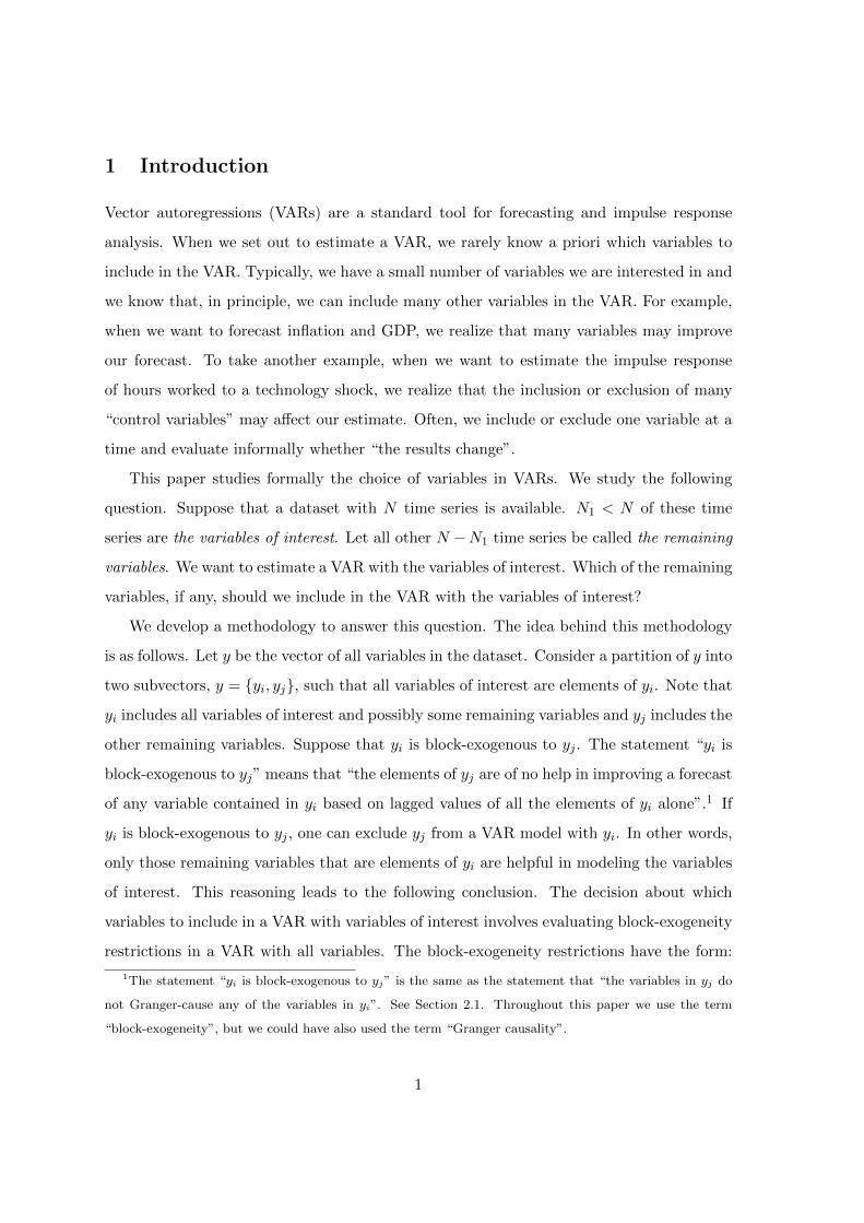
How certain are we that a given variable is to be left out? Table 3 reports, for
each remaining variable in the dataset, the best model in the family Ω with that variable in
the first block. In particular, the posterior odds relative to the best model ω∗ are given. As
Kass and Raftery (1995), we think of the posterior odds between 1 and 0.3 as “not worth
more than a bare mention”, of the odds between 0.3 and 0.05 as “positive”, of the odds
between 0.05 and 0.007 as “strong”, and of the odds below 0.007 as “very strong”.
How strong is the evidence that a given variable is to be left out of the VAR model
with the price level, GDP, and the policy rate? Consider Table 3. The evidence that
the long-term interest rate is to be left out is borderline between “not worth more than
a bare mention” and “positive”. We noted before that the long-term interest rate is the
only variable appearing in Table 1 other than the unemployment rate, the bond spread, the
purchasing managers index, and the federal funds rate. Next, the evidence that the price of
oil, the stock market index, housing investment, the commodity price index, consumption,
and the stock market implied volatility index are to be left out is “positive”. The evidence
that U.S. GDP, loans to non-financial corporations, and the exchange rate are to be left
out is “strong”. The evidence that the house price index and money supply are to be left
out is “very strong”.
The last column of Table 3 shows the remaining variables in the first block of each model
in that table. In all models except one the first block includes the unemployment rate, the
bond spread, the purchasing managers index, and the federal funds rate.36 We see this
finding as consistent with the main finding that the best VAR with the price level, GDP,
and the policy rate in addition includes those four variables.
Single block-exogeneity restriction versus multiple block-exogeneity restric-
tions. The data strongly support imposing multiple block-exogeneity restrictions rather
the “one-unit-root” dummy gradually from 1 (the best model) to 10. The posterior odds relative to the
unrestricted model fall to about 12. Furthermore, the posterior odds of the model ω∗ (with the “one-unit-
root” dummy hyperparameter set to 1) relative to the model with the same block-exogeneity restrictions and
the “one-unit-root” dummy hyperparameter set to 10 are enormous, about 4 × 10¹⁴. The effect of raising
the hyperparameter on the “no-cointegration” dummy to 10 is similar to the effect of reducing the “overall
tightness” hyperparameter to 0.005.36The only exception is the best model with House Prices in the first block.
27

variable (no) odds to ω∗ variables from y2
in the first block
Unemployment Rate 6 1.00 6,8,18,20
Bond Spread BBB 7to10y 8 1.00 6,8,18,20
PMI 18 1.00 6,8,18,20
US Fed Funds Rate 20 1.00 6,8,18,20
Bond Yield 10y 7 0.30 6,7,8,18,20
Oil Price 12 0.17 6,8,12,18,20
Euro Stoxx 16 0.15 6,8,16,18,20
Real Housing Investment 15 0.12 6,8,15,18,20
Real Investment 5 0.09 5,6,8,18,20
Commodity Prices 13 0.07 6,7,8,13,18,20
Real Consumption 4 0.06 4,6,7,8,18,20
VStoxx 17 0.06 6,8,17,18,20
US Real GDP 19 0.03 6,7,8,12,18,19,20
Loans NFC 10 0.03 6,7,8,10,18,20
Effective Exchange Rate 11 0.02 6,8,11,18,20
House Prices 14 0.005 8,12,14,18
M3 9 0.002 4,6,7,8,9,18,20
Table 3: The best model for each variable.
than one block-exogeneity restriction. The posterior odds in favor of the best model ω∗
relative to the model that only has a single block-exogeneity restriction between the first
block in the model ω∗ and the other variables in the dataset is approximately 2 × 10⁷.
Furthermore, we searched for the best model in the restricted family of models Ω′ ⊂ Ω
such that the family Ω′ includes VARs with at most one block-exogeneity restriction. The
posterior odds in favor of the model ω∗ relative to the best model in Ω′ are approximately
104. It turns out that in each of the best 387 models in the family Ω′ the first block includes
the unemployment rate, the bond spread, the purchasing managers index, and the federal
28
funds rate. We find this result reassuring.37
Evidence from subsamples. We repeated the entire analysis in subsamples. First,
we dropped the last four quarters. The results are very similar to the ones described above.
Second, we dropped the last six quarters. The results differ somewhat from the ones de-
scribed above. The main difference is that the price of oil and commodity prices do well in
addition to unemployment rate, the bond spread, the purchasing managers index, and the
federal funds rate. The ranking of the other variables changes, but house prices and money
supply continue to be the worst variables. Third, we split our baseline sample into two
subsamples with the middle of 2007 as the cut-off point. We refer to the subsample with
the data from 1999Q1 to 2007Q2 as “the calm subsample”. We refer to the subsample with
the data from 2007Q3 to 2010Q4 as “the crisis subsample”.38 In both of these subsamples,
medium-size VARs do better than large and small VARs. In both of these subsamples,
money supply, the index of house prices, loans to non-financial corporations, and the ex-
change rate do poorly. In the calm subsample, the following variables do well: the price of
oil, the purchasing managers index, consumption, and U.S. GDP. In the crisis subsample,
the following variables do well: the bond spread and the federal funds rate. Note that the
price of oil, consumption, and U.S. GDP do not make it into the best model in the full
sample. Furthermore, the unemployment rate fails to do well in each subsample separately.
We are not surprised that the findings differ somewhat between the calm subsample and
the crisis subsample, because the two subsamples are quite different from each other. In the
future, it will be useful to redo this paper’s analysis with non-linear models in this particular
sample. In some non-linear models, such as VARs with Markov-switching and VARs with
stochastic volatility, the principle behind the choice of variables will be the same as the
37The MC3 chains that we ran within the family Ω′ quickly gravitate towards models where the two blocks
have approximately the same number of variables. Such models have roughly the maximum number of zero
restrictions possible in a model in the family Ω′.38When analyzing the calm subsample, we use the training sample 1989Q1-1998Q4. Adding this training
sample improves the marginal likelihood in the calm subsample compared with using the Sims-Zha prior
only. When analyzing the crisis subsample, we use the training sample 1999Q1-2007Q2. Adding this training
sample improves the marginal likelihood in the crisis subsample compared with using the Sims-Zha prior
only. Adding this training sample improves the marginal likelihood in the crisis subsample also compared
with using the Sims-Zha prior and the training sample 1989Q1-2007Q2.
29
principle laid out in this paper. However, in a non-linear model computation of marginal
likelihood will be more complex than shown in Section 3.3.
We think of the results reported in this section as an illustration of the methodology
proposed in this paper. We do not want to argue that the results reported in this section
settle once and for all which variables are useful when the interest is in modeling in a VAR
the price level, GDP, and the policy rate in the euro area. The sample available to us is too
short for that and structural breaks may cause different variables to be useful in different
periods.
6 Conclusions
We show how to evaluate conveniently the marginal likelihood implied by a VAR with one
block-exogeneity restriction and multiple block-exogeneity restrictions. One can use these
results in Bayesian tests of block exogeneity – Granger causality – in VARs. We employ
these results to guide the choice of variables to include in a VAR with given variables
of interest. The question of the choice of variables arises in most applications of VARs,
whether in forecasting or impulse response analysis. Typically, the choice of variables occurs
informally. We do not want to argue that the choice of variables must occur formally, using
the methodology of this paper, in each Bayesian VAR from now on. We do want to suggest
that: (i) the choice of variables can occur formally in a straightforward way, and (ii) even
when the choice of variables occurs informally, it is useful to know what formal procedure
this informal choice is meant to mimic.
30

A Sims-Zha prior
The prior used in this paper consists of two components: (i) an initial prior formulated
before seeing any data, and (ii) a training sample prior. See Sections 3.2 and 5.2. This
appendix gives the details concerning the initial prior. See Section 5.2 concerning the
training sample prior.
The initial prior is the prior proposed by Sims and Zha (1998) and consists of the
following four components.
The first component is the modified Minnesota prior. The modified Minnesota prior is
p(vecB|Σ, ωU ) = N
vec
IN
0K−N×N
,Σ⊗WW ′
, (23)
where W is a diagonal matrix of size K × K such that the diagonal entry corresponding
to variable n and lag p equals λ1/(σnpλ2). The terms λ1, λ2, and σn are hyperparameters.
Let P = (1, ..., P ) and σ = (σ1, ..., σN ). Then
W−1 = diag(λ−1
1 P λ2 ⊗ σ, λ−13
),
where λ3 is a hyperparameter associated with the constant term γ. We implement the
modified Minnesota prior with the dummy observations
YLitterman = W−1
IN
0K−N×N
, XLitterman = W−1.
We set σ equal to standard deviations of residuals from univariate autoregressive models
with P lags fit to the individual series in the sample.
The second component of the initial prior is the one-unit-root prior. The one-unit-root
prior is implemented with the single dummy observation
Yone−unit−root = λ4y, Xone−unit−root = λ4(y, ..., y, 1),
where λ4 and y are hyperparameters. We set y = (1/P )P−1∑t=0
y−t, the average of initial values
of y.
The third component is the no-cointegration prior. The no-cointegration prior is imple-
mented with the N dummy observations
Yno−cointegration = λ5 diag(y), Xno−cointegration = λ5(diag(y), ...,diag(y), 0),
31

where λ5 is a hyperparameter.
The fourth component of the initial prior is an inverted Wishart prior about Σ with
mean diag(σ2). This prior is
p(Σ|ωU ) = IW(ZZ ′, ν0) ∝ |Σ|−(ν0+N+1)/2 exp
(−1
2tr(ZZ ′Σ−1
))= |Σ|−(ν0+1)/2|Σ|−N/2 exp
(−1
2tr(Z ′ − 0B
)′ (Z ′ − 0B
)Σ−1
),
where ZN×N and ν0 are hyperparameters. This prior is proportional to a likelihood of N
observations with YΣ = Z ′ and XΣ = 0N×K , multiplied by the factor |Σ|−(ν0+1)/2. We set
Z =√ν0 −N − 1 diag(σi), which implies that the mean of this prior is
E(Σ) =ZZ ′
ν0 −N − 1= diag(σ2
n).
We set ν0 = K + N = N(P + 1) + 1. The reason for this choice for the value of ν0 is as
follows. The inverted Wishart density is proper when ν0 > N − 1. The Sims-Zha prior is
proper when ν0 > K +N − 1, because K degrees of freedom are “used up” by the normal
density of B. Therefore, as a rule of thumb we use the next integer after K +N − 1 setting
ν0 = K +N .
Collecting all dummy observations introduced here yields
YSZ =
YLitterman
Yone−unit−root
Yno−cointegration
YΣ
, and XSZ =
XLitterman
Xone−unit−root
Xno−cointegration
XΣ
.
The matrices YSZ and XSZ appear in expression (22).
We use the following values of the hyperparameters: λ1 = 0.1, λ2 = 1, λ3 = 2, λ4 = 1,
and λ5 = 1. Furthermore, we set the number of lags to 1, that is, P = 1. We explored
the effect of different hyperparameter values and different values of P on the marginal
likelihood of the data implied by the unrestricted VAR estimated on the training sample
1989Q1-1998Q4. We used a grid of values for each of the hyperparameters and we used a
grid of values for the number of lags. We found that the above values of the hyperparameters
and one lag yield the highest value of the marginal likelihood. The values of λ2, λ3, λ4 and
32

λ5 that we found to be optimal are the same as the values used in Sims and Zha (1998). Our
preferred value of λ1 is one-half of the value used by Sims and Zha (1998), which implies
that our prior is tighter. This is consistent with the suggestion of Giannone et al. (2010) to
use tighter priors as the number of variables in the VAR increases.
B MC3
This appendix gives the details concerning the MC3 algorithm that we use. See also Section
3.4.
Given a model ω ∈ Ω, we define the neighborhood of this model denoted nbr(ω). The
neighborhood of a model ω is the set of all models that differ from the model ω by the
position of only one variable in the pattern of block-exogeneity restrictions. For example,
one variable that belongs to the first block in the model ω may instead belong to the second
block in a model ω′ ∈ nbr(ω). In general, the position of a variable can differ in one of four
possible ways: (i) the variable may join the previous block, (ii) the variable may joint the
next block, (iii) the variable may become a block on its own prior to its current block, (iv)
the variable may become a block on its own posterior to its current block. The MC3 chain
moves as follows. Suppose the chain is at a model ω. We attach equal probability to each
model in nbr(ω) and randomly draw a candidate model ω′ from nbr(ω). We accept this
draw with probability
min
1,
#nbr(ω)p(Y |ω′)#nbr(ω′)p(Y |ω)
where #nbr(ω) denotes the number of models in nbr(ω).
When sampling from the family Ω′ we used the convergence criterion proposed in George
and McCulloch (1997). We ran two chains of one million draws. (That is, we drew a
candidate model one million times, but not all of these draws were accepted.) The first
chain started from the unrestricted model. The first chain made 435222 moves and it
visited 13091 models. We saved these 13091 models and, when running the second chain,
we checked how often the second chain visited these same models. The second chain started
from the model where y1 is block-exogenous to all elements of y2. This block-exogeneity
assumption yields the smallest possible first block, in contrast to the unrestricted model
33

which has the largest possible first block. Thus, the second chain started as far as possible
from the first chain, in the sense the number of moves required for the second chain to get
to the starting model of the first chain was at a maximum. The second chain stayed within
the set of the 13091 models from the first chain 99.2% of the time. This suggests excellent
convergence. The inference concerning best models from both chains was exactly the same.
When sampling from the family Ω, we began by examining the properties of the Monte
Carlo described in Section 3.3. We verified that when a model has only one block-exogeneity
restriction – so that we know the marginal likelihood analytically – the Monte Carlo con-
verges to the true value. Next, we checked 20 randomly selected models with multiple
block-exogeneity restrictions. With M = 1000 draws we recovered the marginal likelihood
on average up to a factor of 2, which is an insignificant difference when it comes to com-
paring marginal likelihoods. With M = 10 draws we recovered the marginal likelihood on
average up to a factor of 7, which is a significant difference. We concluded that, given a
time constraint, we faced a trade-off between precision of the Monte Carlo (a large value of
M) and length of the chain. We proceeded in two steps. We first ran an MC3 chain with
one million draws using M = 10. We then collected the best 100,000 models visited by this
chain and we recomputed the marginal likelihood implied by each of those models using
M = 1000.
Satisfying formal convergence criteria when sampling from the family Ω is much more
difficult compared with the family Ω′, for two reasons. First, the family Ω contains many
more models than the family Ω′. Second, very many models in the family Ω differ little from
one another. For example, consider two models with several blocks. Moving one variable
from the last block to the last-but-one block typically produces only a negligible change in
the marginal likelihood. Therefore, we took a pragmatic approach. We ran five independent
chains of length one million with different starting points and we asked if the lessons we
could draw from these chains were the same. We found that the lessons were the same.
Section 5.3 reports results obtained by stacking all five chains together.
Consider detailed examples. In four out of the five chains the best model in that chain
had the same first block as the model ω∗. The exception was that the best model in one chain
included the long-term interest rate in the first block, in addition to the unemployment rate,
34

the bond spread, the purchasing managers index, and the federal funds rate. Furthermore,
on average seven – and at least five – models out of the best ten models in each chain had
the same first block as the model ω∗. In all of the remaining cases the variables from the
first block in the model ω∗ were all present and only one additional variable was present (in
78% of the cases this additional variable was the long-term interest rate).
In the calm subsample and in the crisis subsample the results across chains were some-
what less consistent than in the full sample. We conjecture that in shorter samples the
differences in marginal likelihoods are smaller, and thus probability is distributed more
evenly across models.
Our experience suggests that the search for the best model in the family Ω′ can be
performed quickly and reliably with MC3 even when the number of the remaining variables
in the dataset, N2, is twice larger than in our study. The search for the best model in
the family Ω takes several days, and therefore is feasible today so long as the number of
remaining variables in the dataset, N2, is not much larger than in our study and will become
more and more reliable in larger datasets as computers improve.
35

References
Banbura, M., Giannone, D., and Reichlin, L. (2010). Large Bayesian vector auto regressions.
Journal of Applied Econometrics, 25(1):71–92.
Bauwens, L., Lubrano, M., and Richard, J.-F. (1999). Bayesian Inference in Dynamic
Econometric Models. Oxford University Press, Oxford.
Chib, S. (1995). Marginal likelihood from the Gibbs output. Journal of the American
Statistical Association, 90(432):1313–1321.
Cushman, D. O. and Zha, T. (1997). Identifying monetary policy in a small open economy
under flexible exchange rates. Journal of Monetary Economics, 39(3):433–448.
Dickey, J. M. (1971). The weighted likelihood ratio, linear hypotheses on normal location
parameters. The Annals of Mathematical Statistics, 42(1):204–223.
George, E. I. and McCulloch, R. E. (1997). Approaches for Bayesian variable selection.
Statistica Sinica, 7:339–373.
George, E. I., Sun, D., and Ni, S. (2008). Bayesian stochastic search for VAR model
restrictions. Journal of Econometrics, 142(1):553–580.
Geweke, J. (2005). Contemporary Bayesian Econometrics and Statistics. John Wiley and
Sons, Hoboken, New Jersey.
Geweke, J. and Amisano, G. (2011). Optimal prediction pools. Journal of Econometrics,
164(1):130–141.
Giannone, D., Lenza, M., and Primiceri, G. (2010). Prior selection for vector autoregres-
sions. Discussion paper, Universite Libre de Bruxelles, European Central Bank, and
Northwestern University.
Granger, C. W. J. (1969). Investigating causal relations by econometric models and cross-
spectral methods. Econometrica, 37(3):424–38.
Hamilton, J. D. (1994). Time Series Analysis. Princeton University Press, Princeton, New
Jersey.
36

Kass, R. E. and Raftery, A. E. (1995). Bayes factors. Journal of the American Statistical
Association, 90(430):773–795.
Mackowiak, B. (2007). External shocks, U.S. monetary policy and macroeconomic fluctua-
tions in emerging markets. Journal of Monetary Economics, 54(8):2512–2520.
Madigan, D. and York, J. (1995). Bayesian graphical models for discrete data. International
Statistical Review, 63(2):pp. 215–232.
OEIS (2011). On-line encyclopedia of integer sequences: A000670. Available at
http://oeis.org.
Sims, C. (2010). Lecture notes: causal orderings and exogeneity. Available at
http://sims.princeton.ftp.edu/yftp/times09/addednotes/gcp09.pdf.
Sims, C. A. (1972). Money, income, and causality. American Economic Review, 62(4):540–
52.
Sims, C. A. (1980). Macroeconomics and reality. Econometrica, 48(1):1–48.
Sims, C. A. and Zha, T. (1998). Bayesian methods for dynamic multivariate models. In-
ternational Economic Review, 39(4):949–68.
Waggoner, D. F. and Zha, T. (2003). A Gibbs sampler for structural vector autoregressions.
Journal of Economic Dynamics and Control, 28(2):349–366.
Zha, T. (1999). Block recursion and structural vector autoregressions. Journal of Econo-
metrics, 90(2):291–316.
37
Recommended