© 2011, Samson S. Truong, NASA Dryden Flight Research Center, Edwards, CA, 93523
Conical Probe Calibration and Wind Tunnel Data Analysis
of the Channeled Centerbody Inlet Experiment
A Cooperative Education Experience Assignment & Senior Project
presented to
the Faculty of the Aerospace Engineering Department
California Polytechnic State University, San Luis Obispo
In Partial Fulfillment
of the Requirements for the
Degree of Bachelor of Science
Samson Siu Truong
Spring 2011

1
NASA Dryden Flight Research Center
Conical Probe Calibration and Wind Tunnel Data Analysis
of the Channeled Centerbody Inlet Experiment
Samson S. Truong*
NASA Dryden Flight Research Center, Edwards, CA, 93523
For a multi-hole test probe undergoing wind tunnel tests, the resulting data needs to be
analyzed for any significant trends. These trends include relating the pressure distributions,
the geometric orientation, and the local velocity vector to one another. However,
experimental runs always involve some sort of error. As a result, a calibration procedure is
required to compensate for this error. For this case, it is the misalignment bias angles
resulting from the distortion associated with the angularity of the test probe or the local
velocity vector. Through a series of calibration steps presented here, the angular biases are
determined and removed from the data sets. By removing the misalignment, smoother
pressure distributions contribute to more accurate experimental results, which in turn could
be then compared to theoretical and actual in-flight results to derive any similarities. Error
analyses will also be performed to verify the accuracy of the calibration error reduction.
The resulting calibrated data will be implemented into an in-flight RTF script that will
output critical flight parameters during future CCIE experimental test runs. All of these
tasks are associated with and in contribution to NASA Dryden Flight Research Center’s
F-15B Research Testbed’s Small Business Innovation Research of the Channeled
Centerbody Inlet Experiment.
Nomenclature
CCIE = Channeled Centerbody Inlet Experiment
CFD = Computational Fluid Dynamics
Cs = Static Pressure Coefficient
= Angle of Attack Static Pressure Coefficient
= Sideslip Angle Static Pressure Coefficient
Ct = Total Pressure Coefficient
= Angle of Attack Total Pressure Coefficient
= Sideslip Angle Total Pressure Coefficient
Cα = Angle of Attack/Pitch Pressure Coefficient
= α - Pitch Coefficient Offset
Cβ = Sideslip Angle/Yaw Pressure Coefficient
= β - Pitch Coefficient Offset
DFRC = Dryden Flight Research Center
M = Mach Number
MSFC/ARF TWT = George C. Marshall Space Flight Center Aerodynamic Research Facility 14 × 14-inch Trisonic
Wind Tunnel
NASA = National Aeronautics and Space Administration
Pa = Average of Probe Static Pressures
Po = Wind Tunnel Total Pressure, psi
Ps = Wind Tunnel Static Pressure, psi
P1 = Probe Total Pressure Measured behind Normal Shock at Cone Apex, psi
P2 = Probe Static Pressure to the right of P1, psi
P3 = Probe Static Pressure below P1, psi
P4 = Probe Static Pressure to the left of P1, psi
P5 = Probe Static Pressure above P1, psi
* Student Trainee Engineer Co-op, Aerodynamics and Propulsion Branch

2
NASA Dryden Flight Research Center
Qbar = Pseudo/Probe Dynamic Pressure, psi
Qbar - true = True Dynamic Pressure, psi
RTF = Real-Time Fortran
SBIR = Small Business Innovation Research
= Local Velocity Vector
Xp = X-axis of Probe Coordinate System
Yp = Y-axis of Probe Coordinate System
Zp = Z-axis of Probe Coordinate System
α = Angle of Attack/Pitch Angle, deg
αo = Vertical Misalignment Angle with Probe Rotated 0° and 180°, deg
β = Sideslip Angle/Yaw Angle, deg
βo = Vertical Misalignment Angle with Probe Rotated ± 90°, deg
γ = Ratio of Specific Heats
δ = Uncertainty
θ = Pitch Angle, deg
φ = Roll Angle, deg
I. Introduction
UPERSONIC and hypersonic vehicles require inlets with an efficient geometric design that would provide
suitable air mass flow into its engines for better low Mach number flight operations. At low supersonic
conditions, inlets must be able to provide a substantial amount of transonic airflow in order to meet the engines’
demand. As a result, a large inlet throat area is required to fulfill this requirement. This could potentially allow for
higher efficiency engine combined cycle propulsion systems, such as the Rocket-Based Combined Cycle (RBCC)
and the Turbine-Based Combined Cycle for supersonic cruise or hypersonic acceleration. Research into this area is
currently underway with the Channeled Centerbody Inlet Experiment (CCIE), as seen in Fig. 1, at the NASA
Dryden Flight Research Center in conjunction with the TechLand Research Incorporation through NASA’s Small
Business Innovation Research (SBIR) contract. 1
The overall objective of the CCIE research is to investigate the off-design performance of a supersonic inlet with
a variable geometry at varying Mach test points. The two primary factors that researchers hope to derive from this
study is the inlet flow of both the channeled centerbody and the equivalent area smooth centerbody and how well the
flight results compare to the CFD calculations. The channeled centerbody, shown in Fig. 2a, has grooved channels
along the centerbody to enhance flight at off-design
conditions. These grooves or channels in the centerbody
allow for additional throat area to increase the amount of
mass flow coming into the inlet during off-design flight.
The benefit of having these grooves results in lower
internal compression, which allows an aircraft designer
to select a mixed-compression inlet configuration often
used for high supersonic and hypersonic applications
due to its high total pressure recovery and desired high-
speed cruise performance. The equivalent smooth
centerbody, shown in Fig. 2b, however, has no grooves.
The absence of these grooves means that the throat area
is smaller and aircraft designers must choose an inlet
with high internal compression in order to provide the
amount of mass flow the engine needs at off-design
conditions. This option means the designer has to risk
the high probability of inlet unstart and low operability
since this type of inlet with a fixed-geometry requires
overspeeding.1-2
With flight testing, researchers hope to
find out the overall performance of the channeled
centerbody and how it compares to the equivalent
smooth centerbody. It should be noted that TechLand’s
concept is a translating channeled centerbody capable of
changing the cross-sectional area geometry, while the
S
Figure 1. The Channeled Centerbody Inlet
Experiment (CCIE) is shown here as the gold
structure mounted underneath the black
Propulsion Flight Test Fixture (PFTF), which in
turn is attached to the F-15D centerline pylon
through two suspension lugs so that all the loads
are transferred to the aircraft.

3
NASA Dryden Flight Research Center
one being tested at NASA DFRC is a fixed geometry design. If the flight results provide results as expected, the
channeled centerbody inlet concept could potentially be implemented for both commercial and space applications in
the near future, ranging from supersonic transports to space-access vehicles.
Prior to any flight testing, one of the tests that prepared the CCIE was a wind tunnel test that obtained data for
the 5-hole pressure probes, 4 static and 1 total, located near the nose cone apex, shown in Fig. 3 mounted in the test
section. In addition, the conical probe has a 16° cone semivertex or half-angle. The wind tunnel test was conducted
in June 2010 at the George C. Marshall Space Flight Center Aerodynamic Research Facility 14 × 14-inch Trisonic
Wind Tunnel (MSFC/ARF TWT), which recently upgraded its facility with a new data acquisition and tunnel
control system. The MSFC/ARF TWT is an intermittent blow-down tunnel where high-pressure air from outside
storage tanks flows through a diffuser, a heat exchanger, and into one of two test sections, the transonic or the
supersonic test sections. The transonic test section is capable of producing Mach numbers ranging from 0.2 to 2.5,
whereas the supersonic test section produces Mach numbers from about 2.7 to 5.0.4 For this particular test, the
transonic test section was utilized as the CCIE’s intent is to investigate off-design low supersonic conditions. The
test points included testing at Mach numbers 1.2, 1.3, 1.46, and 1.69, and for each test point, the probe was set at roll
angles, φ of 0°, 90°, 180°, and -90° with positive angle
representing counterclockwise rotation and negative
angles representing clockwise rotation. In addition,
pitch sweeps were conducted at each Mach condition to
gather measurements for angle of attack, α and angle of
sideslip, β. The test section is only capable of
traversing in the vertical direction and as a result,
sideslip had to be measured as pitch maneuver, not a
yaw horizontal maneuver. The wind tunnel test resulted
in data that was used later for calibration of flow
angularity in the pitch and yaw planes as well as the
Mach number values that the pressure probes were
reading. 5
During the wind tunnel test of the CCIE’s 5-hole
pressure probe, it was not expected that the test article
would remain stationary at one set location and neither
the local velocity vector will be aligned, causing
variations in the positioning of the two. Small
angularities contributed to the misalignment of either
the probe or the local velocity vector and therefore,
(a) (b)
Figure 2. The channeled centerbody (a) and the equivalent smooth centerbody (b) are two of the
centerbodies that will be tested for the Channeled Centerbody Inlet Experiment (CCIE) .3 Notice that the
channeled centerbody has grooves providing more inlet area as opposed to the equivalent smooth
centerbody. The channeled centerbody was designed ideally for Mach 1.5 conditions.
Figure 3. The nose apex of the CCIE is where the 5-
hole pressure probe is located and is mounted here
in the MSFC/ARF TWT transonic test section.

4
NASA Dryden Flight Research Center
creates an angular bias that needs to be addressed in the calibration.6 As a result, calibration correction of the wind
tunnel data for all the Mach number test points needs to be performed in order to determine the relationships
between the measured pressures, the probe’s geometric orientation, and the local velocity vector. The conical
calibration and error reduction process of the CCIE wind tunnel data will produce calibration graphs from which
they could be compared to one another to derive any significant trends amongst pressure and angular parameters in
the low supersonic regime.
II. Conical Probe Calibration Wind Tunnel Data Analysis & Procedures
The conical probe calibration of the CCIE will consist of several major steps, each of which is critical to the
accuracy of the outcome of the calibration. These steps include identifying the key probe parameters and a
coordinate system for reference purposes, calculating pressure coefficients of interest to the calibration, the conical
calibration process itself detailing how misalignments are calculated
and how they are dealt with, and the error and uncertainty analysis
post-calibration process. Eventually, the calibrated data and its maps
will be used to construct an in-flight RTF code to output desired data in
real-time during the CCIE’s experimental flight on the F-15B research
aircraft.
A. Establish the Probe Parameters and the Coordinate System
Prior to performing the calibration and error reduction, multiple
parameters need to be defined in order to have a clear understanding of
how to perform the calculations. First, the CCIE multi-hole pressure
probes have to be labeled for reference purposes. This particular multi-
hole probe has 5 ports, one measuring the total pressure and the other
four measuring the static pressure. In Fig. 4, the total pressure port is
located in the center amongst the other ports and is designated as P1.
The other ports surrounding P1 are the static pressure ports. Starting at
the right of P1 and going clockwise, the ports are labeled as P2, P3, P4,
and P5. The pressure measurements from these ports will allow non-
dimensional pressure coefficients to be calculated later on. Utilizing a multi-hole pressure probe, also called an
impact probe, allows more data collection capability than a standard pitot probe as it now could measure the
direction of the flow velocity in three dimensions.
In order to establish any angular parameters,
such as angle of attack and roll angle, the probe’s
position needs to be identified with a coordinate
system. During the wind tunnel test and data
collection, the probe’s position is assumed to be
fixed in space. The velocity vector’s orientation
will be measured with respect to the probe’s fixed
coordinate system. In Fig. 5, the probe coordinate
system is shown with axes Xp, Yp, and Zp with the
probe aligned along the Xp-axis. The probe tip
meets with the incoming local velocity vector, at
the origin. Several angles that indicate the position
of the probe in relation to the local velocity vector
include angle of attack, α, sideslip angle, β, pitch
angle, θ, and roll angle, φ. The angle of attack or
the pitch angle is the angle that the probe makes
with respect to the oncoming flow about the Yp-axis.
The sideslip angle or the yaw angle is the angle that
the probe makes with the local velocity vector about
the Zp-axis.7 Finally, the roll angle is the angle that
the probe twists about its centerline on the Xp-axis.
Figure 4. Looking head on, the
CCIE multi-hole pressure probe is
arranged in this manner for roll
angle φ = 0°. The probe, P1
measures the total pressure, while
the remaining probes P2, P3, P4, and
P5 measure the static pressure.
Figure 5. The probe coordinate system is illustrated
above with the probe aligning along the Xp –axis. The
four angles of interest, angle of attack, α, sideslip
angle, β, pitch angle, θ, and roll angle, φ are shown
here and help in determining the orientation of both
the probe and the local velocity vector.

5
NASA Dryden Flight Research Center
B. Calculate the Pressure Coefficients
With the pressure ports identified, an established coordinate system, and angular parameters defined, the data
obtained from these independent variables can be used to determine the unknown dependent variables.8 These
dependent variables consist of mostly pressure coefficients, which are later plotted against angles of interests and
other pressure coefficients to determine behavioral trends in pressure due to different pitch and roll angles at a
particular Mach number. Pressure coefficients are significant as they describe the relative pressures about a point, in
this case, the probe in a fluid flow field. To determine these pressure coefficients, one variable needs to be
calculated that will assist in non-dimensionalizing all of the pressure coefficient variables. This variable is the
average probe static pressure, Pa and is equal to the arithmetic mean of the four measured static pressures on the
multi-hole probe. It can be calculated as
. (1)
The first pressure coefficient to be calculated is Cα, the angle of attack or the pitch pressure coefficient. During
wind tunnel measurements of the multi-hole pressure probe, Cα is associated with roll angles of φ = 0° and φ = 180°.
By looking at the probe’s orientation in Fig. 4, these two roll angles align with pressure probes P1, P3, and P5.
Therefore, Cα was calculated as the difference between the two static pressures non-dimensionalized by the
difference between the total and average static pressures or simply as
. (2)
The non-dimensionalization by the denominator, P1 - Pa in Eq. 2 is actually the pseudo or the probe dynamic
pressure based on initial measured pressures and can be represented as Qbar. Replacing the denominator in Eq. 2
with the freestream dynamic pressure gives the revised Cα formula in Eq. 3 as
. (3)
The MSFC/ARF TWT’s probe holder cannot traverse in the horizontal direction and as a result, data collection for
sideslip maneuvers involves the probe being rotated at roll angles of φ = 90° and φ = -90°. Subsequently, the
sideslip angle or the yaw pressure coefficient, Cβ was calculated in the same manner, this time along the horizontal
axis probes, P1, P2, and P4 as shown here in Eq. 4 as
(4)
The total pressure coefficient, Ct is the ratio between the difference in total pressures of the probe, P1 and the wind
tunnel freestream condition, Po and the freestream dynamic pressure, Qbar. This relation is represented in Eq. 5 as
(5)
Similarly, the static pressure coefficient, Cs was calculated as the difference between the difference in the total
pressure of the probe, P1 and the wind tunnel static pressure, Ps non-dimensionalized by the freestream dynamic
pressure, Qbar. Subtracting out Ps eliminates the static pressure component of the probe total pressure. Thus, Cs was
written in Eq. 6 as
(6)
With all of the necessary pressure coefficients calculated, relationships were established between other parameters
of interest, such as angle of attack and sideslip angle throughout the calibration process.

6
NASA Dryden Flight Research Center
C. Determine the Vertical Misalignments
Data collection for angle of attack and sideslip angle were both gathered from the MSFC/ARF TWT test as a
vertical pitch maneuver since the probe holder in the wind tunnel was not able to traverse in the horizontal direction.
Therefore, the discussion here will focus only on the vertical misalignment case as opposed to the horizontal
misalignment case. To assume that the probe is perfectly aligned with the flow field is an assumption that should
never be made. In order to visualize the misalignment, plots were created for both the angle of attack and sideslip
angle cases by plotting them with their respective dependent variable angle of attack and sideslip pressure
coefficients, Cα and Cβ. This was done for each of
the Mach test points of 1.2, 1.3, 1.46, and 1.69. For
simplicity purposes, graphs at Mach 1.2 will be
displayed here, while the remaining test points’
graphs could be viewed in the Appendix since their
trends are similar.
In Fig. 6a, Cα is plotted against angle of attack, α
at roll angles, φ = 0° and φ = 180°, while in Fig. 6b,
Cβ is plotted against the sideslip angle, β at roll
angles of φ = 90° and φ = -90°. For both cases, Cα
and Cβ vary linearly with their respective angles
with each data point having an associated error
bound to it. Due to the error associated with each
data point during the wind tunnel test, the data
points are of course not in a perfect straight linear
line. As a result, the data points for each roll angle
need an associated line of best fit, since in theory the
pressure coefficients, Cα and Cβ are linearly related
to their corresponding angles, α and β. For φ = 0°,
the line of best fit for the pressure coefficient, Cα can
be calculated as
(7)
where m1 is the slope of the best fit line of Cα at φ =
0°, α is the angle of attack, and αφ ° α ° is the y-
intercept of the pressure coefficient when α = 0°.
Likewise, at φ = 180°, Cα is calculated in Eq. 8 as
(8)
with m2 being the slope of the best fit line.
Similarly, the sideslip case in Fig. 6b at φ = 90° and
φ = -90° can have their lines of best fit for the
pressure coefficient, Cβ written in Eq. 9 and 10 as
(9)
(10)
where n1 and n2 are the slopes of the best fit lines for
βφ ° and
, respectively. Notice that the
best fit lines for Cα at φ = 0° and φ = 180° and the
best fit lines for Cβ at φ = 90° and φ = -90° cross one
another in Fig. 6a and 6b since the slopes are almost
equal in magnitude.
(a)
(b)
Figure 6. For the Mach 1.2 test point, pressure
coefficients, Cα and Cβ are plotted with their
corresponding vertical pitch angles, α and β,
respectively. Cα values at φ = 0° and φ =180° as well as
Cβ values at φ = 90° and φ =-90° intersect one another,
varying linearly and are about equal in magnitude. α
and β values range from ±6°, while Cα and Cβ values
ranged from about -0.08 to 0.08. The small pressure
coefficient value suggests high dynamic pressure at this
particular test point.

7
NASA Dryden Flight Research Center
The intersection of the two lines indicates the point where Cα and Cβ remains constant regardless of roll angle, as
well as dictates the orientation the probe is aligned with the local velocity vector. Also, this point is important as it
determines the vertical misalignment angle, αo and βo, and the α and β-pitch coefficient offsets, and
.
Remember that the probe in the wind tunnel cannot traverse in the horizontal direction and as a result, βo and
will be treated as a vertical pitch maneuver. Theoretically, the intersection of the two lines should rest at the origin
with αo and βo equaling zero and Cα(0) and Cβ(0) should equal zero as well. This assumes the probe in the wind
tunnel is fixed in space and exactly aligned with the local velocity vector, requiring an accurate knowledge of the
incoming flow angularity. In addition, the theoretical condition assumes that the probe is symmetrically machined
with precision, in which the static pressure ports, P2, P3, P4, and P5 are drilled equidistance from the probe tip,
resulting in equal static pressure values when exactly aligned with the flow field.9 However, in reality, these
assumptions often do not hold true. As a result, vertical misalignment angles and pitch coefficient offsets are
present and need to be calculated. Eventually, the vertical misalignment will be removed from the wind tunnel data
to enhance the calibration results. To calculate the vertical misalignment angle, αo from Fig. 6a, Eq. 7 and Eq. 8 are
set equal to each other as this is the intersection point as shown in Eq. 11,
. (11)
Solving for α in Eq. 11 results in the vertical misalignment angle, αo in Eq. 12
, (12)
which is then substituted into Eq. 13 to solve for the α – pitch coefficient offset, α as shown here
. (13)
The same procedures could be then applied to calculate the vertical misalignment angle, βo and its corresponding β –
pitch coefficient, β as shown in Fig. 6b. By setting Eq. 9 and Eq. 10 equal to one another as shown in Eq. 14,
(14)
and solving for β, the vertical misalignment for the sideslip case could be calculated through Eq. 15,
. (15)
Substituting βo into Eq. 16,
(16)
results in the β – pitch coefficient, β . Both the α and β – pitch coefficient offsets take into account of the aligning
errors of the probe in the wind tunnel setup, as well as the asymmetric probe geometry when the probe was
machined.
These misalignment calculations were done for each of the four Mach conditions of interest to understand how
both the angle of attack and sideslip angle behaved in the wind tunnel compared to the theoretical case. Remember
that the theoretical condition assumes perfection in alignment and probe geometry, resulting in absolutely no
misalignment and in turn the pitch coefficient offsets would be zero. In Table 1, the vertical misalignment angles
and the pitch coefficient offsets for both the angle of attack and the sideslip angle are listed with their corresponding
Mach test points. The value for vertical misalignment angles, αo and βo vary with Mach number. Mach 1.3’s
vertical misalignment values of -1.0° ± 0.2° and -1.2° ± 0.2° were off the most in magnitude compared to Mach
1.46’s case of 0.3° ± 0.2° and 0.4° ± 0.2°. The further away the misalignment angle’s magnitude is from zero, the
more bias there will be from the experimental run. Since it is known that the same probe was used throughout,
geometry therefore is consistent with each test, implying that flow conditions and alignment of the probe
significantly affected the vertical misalignment values. It should be noted that these wind tunnel tests were

8
NASA Dryden Flight Research Center
conducted over several days and aligning the probe could introduce small bias to the resultant data. For the pitch
coefficient offsets, and
, a descending trend is noted with increasing Mach number. From Eq. 3 and Eq. 4, at
high supersonic speeds, the dynamic pressure, Qbar increases due to an increase in both the static and total pressures.
The pressure coefficient is related to the inverse of dynamic pressure and as a result, high Mach situations build up
dynamic pressure, resulting in low pressure coefficient values.
D. Remove Vertical Misalignment from Data
In order to create calibration maps of the pressure coefficient relation to its angular counterpart, the vertical
misalignment angle or angular bias has to be eliminated. Typically, this is done through a series of angular rotations
and transformations of the probe about its axes to derive the incoming velocity components prior to rotation.10
However, this particular calibration won’t be looking into detail at the incoming flow, but rather preparing corrected
data to be used for in-flight real-time data collection. Removal of the angular bias is quite simple by taking the
angle of attack and the sideslip angle and subtracting out its vertical misalignment angle, αo and βo, respectively.
This results in a corrected value of angle of attack, αcorrected, and sideslip angle, βcorrected as shown here in Eq. 17 and
Eq. 18:
(17)
. (18)
The Cα and Cβ plots with their respective angles are shown below in Fig. 7a and 7b with the misalignment angle
removed for Mach 1.2 conditions. This means the intersection of the two roll angle data lines now sits on the α and
β-axes at 0°. Essentially, this allows the pressure coefficient values to behave more like the theoretical conditions in
the calibrated data.
Table 1. The values of vertical misalignment angles, αo and βo and their respective pitch coefficient offsets,
and
are shown here at different Mach test point conditions.
MACH αo (deg) βo (deg)
1.20 0.6 ± 0.2 -0.008 ± 0.002 0.7 ± 0.2 -0.003 ± 0.001
1.30 -1.0 ± 0.2 -0.005 ± 0.003 -1.2 ± 0.2 -0.0023 ± 0.0003
1.46 0.3 ± 0.2 -0.004 ± 0.001 0.4 ± 0.2 -0.001 ± 0.001
1.69 0.7 ± 0.2 -0.001 ± 0.002 0.8 ± 0.2 -0.001 ± 0.001
(a) (b)
Figure 7. The pressure coefficients, Cα and Cβ are plotted with their corresponding vertical pitch angles, α
and β, respectively for Mach 1.2 conditions with the vertical misalignment angle removed for each case.
Notice the shift at the intersection point as it aligns at αcorrected = 0° and βcorrected = 0°.

9
NASA Dryden Flight Research Center
E. Determine Pitch and Yaw Angle Polynomials
Two important in-flight parameters that need to be monitored during experimental test flights are angle of attack,
α, and sideslip angle, β, which are essentially the pitch and yaw motions on an aircraft, respectively. The in-flight
real-time Fortran (RTF) script must include equations on how to calculate these two angles, but from Fig. 7, it looks
as if there are a set of two equations for both angle of attack at φ = 0° and 180° and sideslip angle at φ = 90° and
-90°. This is because at roll angles, φ = 180° and φ = -90°, the probe is oriented to measure in the negative
orientation 180° apart from its positive orientation of φ = 0° and φ = 90°, respectively. Looking at the multi-hole
pressure probe arrangement in Fig. 4, to measure the angle of attack, the pressure probe is positioned at φ = 0°, with
pressure ports P5 located at the top and P3 located at the bottom. Likewise, measuring sideslip involves positioning
the probe at φ = 90°, with pressure ports P2 located at the top and P4 located at the bottom, since the wind tunnel has
no horizontal movement capability. At φ = 180°, angle of attack is measured with pressure ports P5 and P3 being
switched with one another and this is the same with sideslip measurements at φ = -90° with P2 now measuring at the
bottom and P4 at the top. Since α and β are measured in the negative orientation at φ = 180° and φ = -90°, their data
values must be multiplied by negative one. Usually, angular transformations are done to correct the orientation, but
since these roll angles are orthogonal, the correction process was simplified. In summary, the pitch angle, θ at φ =
0° and φ = 90° are equal to α and β, respectively, whereas at φ = 180° and φ = -90°, θ is equal to –α and –β.
With the negative orientation at roll angles φ = 180° and φ = -90° accounted for, Cα and Cβ are both plotted again
for all Mach test points with their respective angles of α and β, this time with both the original and the corrected data
with the vertical bias removed. Below in Fig. 8a and 8b, the pressure coefficients are plotted against their
corresponding angles for the Mach 1.2 test condition. Notice that for both plots that the corrected data are
independent of roll angle. For both the angle of attack and sideslip angle scenarios, their corrected angles with the
vertical misalignment eliminated, αcorrected and βcorrected, are more closely packed together, forming a nice linear trend.
From Table 1, it can be inferred that the Mach test points with lower vertical misalignment values of αo and βo will
have both their original and corrected α and β values closer in proximity to each other, such as Mach 1.46 as
opposed to Mach 1.3 with the highest values of αo and βo. The plots for the Mach 1.3, 1.46, and 1.69 case could be
viewed in the Appendix for reference.
The linear trend produced by the graphs in Fig. 8 between the pressure coefficients and the corrected α and β data
is much better than that of the original data, but the corrected data is still slightly off as some data points don’t
necessarily follow in a straight line. Knowing that both the pressure coefficients, Cα and Cβ and their respective
angles, α and β are linearly related, a line of best fit could therefore be used to represent the theoretical angle of
attack and sideslip angle based on the wind tunnel data. By making αcorrected and βcorrected the dependent variable in
(a) (b)
Figure 8. For the Mach 1.2 test point, the pressure coefficients, Cα and Cβ are plotted against their
respective angles, α and β, with their original data with the misalignment and the corrected data with the
misalignment removed. With both the corrected data taking into account of the negative orientation at roll
angles φ = 180° and φ = -90°, the pressure coefficient relationship with their pitch and yaw angles are now
essentially independent of roll angle and vary linearly.11

10
NASA Dryden Flight Research Center
the graphs in Fig. 8, solving for these dependent variables is simple by using MATLAB’s data fitting tool. Figure 9
displays the line of best fit between the corrected angle of attack and sideslip angle with their corresponding
pressure coefficients at Mach 1.2 conditions.
With the aid of MATLAB, the remainder test points had their pitch and yaw angle polynomials calculated at
Mach 1.3, 1.46, and 1.69. Table 2 shows the list of angle of attack and sideslip angle equations for each of the
associated Mach test points. These equations will be used in conjunction with other equations developed along the
way to create the in-flight RTF script for the CCIE. The CCIE’s focus is in the supersonic regime primarily between
Mach 1.2 and Mach 1.69. The RTF code will eventually have to interpolate the solutions between each equation in
order to get the angle of attack and the sideslip angle values that are not exactly right at the calibration Mach test
point. This will be furthered discussed in detail later on in this report.
F. Determine Total and Static Pressure
Coefficient Polynomials
The total pressure coefficient, Ct and
static pressure coefficient, Cs were
previously calculated in Eq. 5 and 6. The
task now is to find a relationship that
relates these two pressure coefficients as a
function of the pitch pressure coefficient,
Cα and the yaw pressure coefficient, Cβ.
The procedure for this is similar to the
previous section on determining the pitch
and yaw coefficient polynomials. The
trends in both the total pressure
coefficient as well as the static pressure
coefficient for all the Mach test conditions
will be compared to the theoretical case to
see how well the wind tunnel test results
did. The resulting wind tunnel results will
be then fitted to formulate equations for Ct
and Cs that will then be incorporated into
the in-flight RTF code.
(a) (b)
Figure 9. The lines of best fit are shown here between the αcorrected and Cα plot (a) and the βcorrected and Cβ
plot (b). This linear fit curve represents the theoretical angle of attack and sideslip angle equations as a
function of pressure coefficients based on the wind tunnel data obtained. These equations will eventually be
implemented with the in-flight RTF script as α = α (Cα) and β = β (Cβ).
Table 2. The pitch and yaw angle polynomials are shown in this
table for each of the Mach number test points. All of these
equations were derived based on the linear line of best fit
between αcorrected and Cα as well as between βcorrected and Cβ.
These equations are to be utilized in the in-flight RTF code to
calculate both the angle of attack and sideslip angle.
MACH α β
1.20 89.1385Cα + 0.7089 90.4277Cβ + 0.2841
1.30 94.6015Cα + 0.5037 100.0237Cβ + 0.2179
1.46 108.0175Cα + 0.4175 112.3877Cβ + 0.1192
1.69 99.9231Cα + 0.1318 100.8961Cβ + 0.0871
11
NASA Dryden Flight Research Center
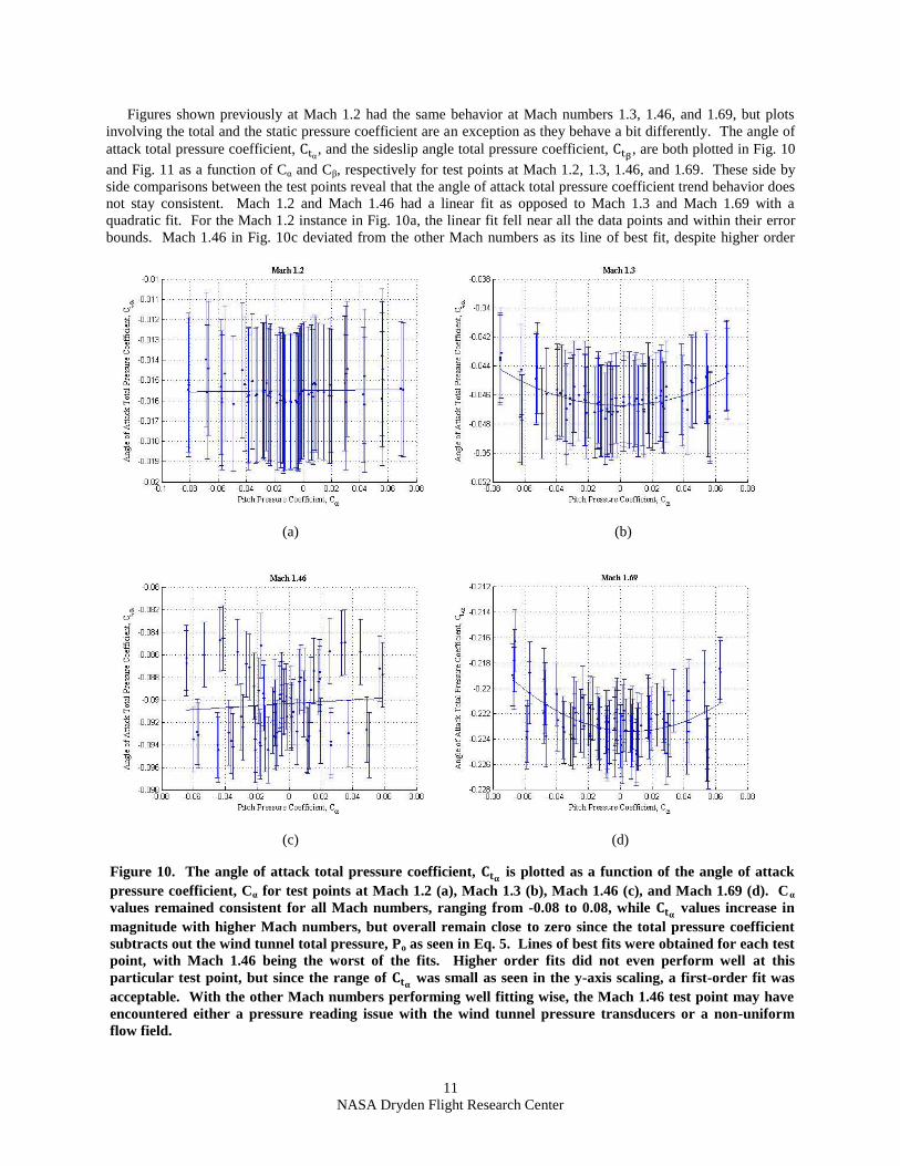
Figures shown previously at Mach 1.2 had the same behavior at Mach numbers 1.3, 1.46, and 1.69, but plots
involving the total and the static pressure coefficient are an exception as they behave a bit differently. The angle of
attack total pressure coefficient, α, and the sideslip angle total pressure coefficient,
, are both plotted in Fig. 10
and Fig. 11 as a function of Cα and Cβ, respectively for test points at Mach 1.2, 1.3, 1.46, and 1.69. These side by
side comparisons between the test points reveal that the angle of attack total pressure coefficient trend behavior does
not stay consistent. Mach 1.2 and Mach 1.46 had a linear fit as opposed to Mach 1.3 and Mach 1.69 with a
quadratic fit. For the Mach 1.2 instance in Fig. 10a, the linear fit fell near all the data points and within their error
bounds. Mach 1.46 in Fig. 10c deviated from the other Mach numbers as its line of best fit, despite higher order
(a) (b)
(c) (d)
Figure 10. The angle of attack total pressure coefficient, is plotted as a function of the angle of attack
pressure coefficient, Cα for test points at Mach 1.2 (a), Mach 1.3 (b), Mach 1.46 (c), and Mach 1.69 (d). Cα
values remained consistent for all Mach numbers, ranging from -0.08 to 0.08, while values increase in
magnitude with higher Mach numbers, but overall remain close to zero since the total pressure coefficient
subtracts out the wind tunnel total pressure, Po as seen in Eq. 5. Lines of best fits were obtained for each test
point, with Mach 1.46 being the worst of the fits. Higher order fits did not even perform well at this
particular test point, but since the range of was small as seen in the y-axis scaling, a first-order fit was
acceptable. With the other Mach numbers performing well fitting wise, the Mach 1.46 test point may have
encountered either a pressure reading issue with the wind tunnel pressure transducers or a non-uniform
flow field.

12
NASA Dryden Flight Research Center
attempts, had trouble acquiring a noticeable trend. Since α data values at Mach 1.46 only differ from one another
by a few thousandths, it was decided a first-order linear fit should work fine. The purpose of the line fitting is not to
connect all the wind tunnel data points, but rather obtain a trend that best describes the behavior at that test
condition.
The similar behavior observed as seen in Fig. 10 could be seen in Fig. 11 with the sideslip angle total pressure
coefficient, plotted as a function of the yaw pressure coefficient, Cβ for all the Mach number test points. Again,
Mach 1.2 and 1.46 were fitted linearly, while Mach 1.3 and 1.69 had a quadratic fit. In addition, values were
comparable to that of . This will help in the approximation of a single total pressure coefficient, Ct value later on
when computing the desired flow properties. At Mach 1.2, both lines of best fit for α and
shown in Fig. 10a
and Fig. 11a suggest a mean value between -0.015 and -0.016. Mach 1.3 and Mach 1.69 conditions for both the
angle of attack and sideslip angle total pressure coefficients showed a decrease in magnitude at the end limits of
their pitch and yaw pressure coefficients. Mach 1.46, however, demonstrated a similar behavior as seen in Fig. 10c
may have been caused by either a pressure reading issue, a flow disturbance due to a non-uniform flow field, or
(a) (b)
(c) (d)
Figure 11. The sideslip angle total pressure coefficient, is plotted as a function of the angle of attack
pressure coefficient, Cα for test points at Mach 1.2 (a), Mach 1.3 (b), Mach 1.46 (c), and Mach 1.69 (d).
Notice the similarity in the trends and values between the sideslip angle and angle of attack total pressure
coefficient figures.

13
NASA Dryden Flight Research Center
experiencing a resonating frequency. This will be further looked into later on by the CCIE aerodynamicists.
Static pressure coefficient trends for all the test points resulted in a similar concave down behavior for both the
angle of attack and the sideslip angle cases. Below in Fig. 12, the angle of attack static pressure coefficient, is
plotted in variation with the pitch pressure coefficient, Cα for all the four Mach test conditions. With increasing
Mach number, the freestream wind tunnel static pressure, Ps decreased, while the dynamic pressure increased. From
Eq. 6, this resulted in lower values of the static pressure coefficient as the Mach number goes higher. The wind
tunnel results have values around a value of one, which is expected based on Eq. 6. Based on Fig. 12 for all test
points, slightly lower values of occurred at the low and high ends of Cα. When these graphs were fitted, a
quadratic fit was used for Mach 1.2, 1.3, and 1.69, while Mach 1.46 with its steeper concave down trend required a
cubic fit for higher accuracy. Much of the data points along with their error bars fell within reach of the lines of best
fit. Since these low order fits were capable of matching the angle of attack static pressure coefficient’s trends, other
higher order fit polynomials were not needed.
(a) (b)
(c) (d)
Figure 12. The angle of attack static pressure coefficient, is plotted as a function of the pitch pressure
coefficient, Cα for Mach 1.2 (a), Mach 1.3 (b), Mach 1.46 (c), and Mach 1.69 (d). The plots here involving
the static pressure coefficient observed a more comparable behavior amongst all the test points with its
concave down trend fit. Values of increased with ascending Mach number varying anywhere between
1.03 and 1.095.

14
NASA Dryden Flight Research Center
Like , the sideslip angle static pressure coefficient,
behaved similarly as plotted in Fig. 13 for all the four
Mach conditions as a function of the yaw pressure coefficient, Cβ. Trends in the best fit lines and the ranges of
values for are analogous to that of the angle of attack case. Comparing the angle of attack and the sideslip angle
case for the total pressure coefficient plots in Fig. 10 and 11 and the static pressure coefficient plots in Fig. 12 and
13 evidently reveal that regardless of the probe orientation, the values of total pressure coefficient and static pressure
coefficient hardly changed between the angle of attack and the sideslip angle scenario. So far, these graphs have
been analyzed separately as the total pressure coefficient and the static pressure coefficient cases with respect to
their corresponding angular pressure coefficients. Since their data points vary by mere tenths or thousandths of a
decimal place, the resulting lines of best fit trends could only be viewed up close. If the these coefficients, total and
static, were plotted simultaneously on the same graph with their respective pitch and yaw pressure coefficients, Cα
and Cβ, resultant horizontal linear lines of no slope would represent the values of the total and static pressure
coefficients as near 0 and 1, respectively. This distinctive trend could be viewed in Fig. 14. With the same exact
behavior seen at every Mach test situation, only Mach 1.2’s and Mach 1.46’s trends will be shown due to their
(a) (b)
(c) (d)
Figure 13. The sideslip angle static pressure coefficient is plotted as a function of the yaw pressure
coefficient, Cβ for Mach 1.2 (a), Mach 1.3 (b), Mach 1.46 (c), and Mach 1.69 (d). For each Mach test point,
their figures are close in likeness to that of their counterparts in the angle of attack case in Fig. 12. Mach
test points 1.2, 1.3, and 1.69 were fitted with a 2nd
order best fit, whereas Mach 1.46 was fitted with a 3rd
order trend line.

15
NASA Dryden Flight Research Center
differing behavior in the total and static pressure coefficient graphs for both the angle of attack and sideslip angle
cases. The graphs for Mach 1.3 and Mach 1.69 can be seen in the Appendix for reference. The static and total
pressure coefficients, Cs and Ct are plotted together as a function of the pitch and yaw pressure coefficients, Cα and
Cβ for Mach 1.2 in Fig. 14a and Fig 14b and for Mach 1.46 in Fig. 14c and Fig 14d, respectively. From the figures,
there are two distinct horizontal lines, with the static pressure coefficients, and , aligning a little bit above a
value of one due to dominance of the higher total pressure values and the total pressure coefficients, and
,
aligning slightly below zero, since P1 ≠ Po in supersonic conditions due to likely pressure differentials across
shockwaves. Even with the multi-hole probe being rotated in the wind tunnel, the independence of roll angle is
shown here with all the data point values having nearly identical values.
With this verification that the static and total pressure coefficient are behaving as they are supposed to be from
this perspective, the total and static pressure coefficient polynomials for both the angle of attack and sideslip angle
instances need to be compiled. These equations will later be used to calculate initial flow properties of interest to
verify the calibration procedure thus far and will of course be integrated with the in-flight RTF script.
(a) (b)
(c) (d)
Figure 14. For Mach 1.2 (a & b) and Mach 1.46 (c & d), both their angle of attack and sideslip angle static
and total pressure coefficients, ,
, , and
, are plotted with their respective angular pressure
coefficients, Cα and Cβ. From this different vantage point, one can note the independence of roll orientation
in terms of the total and static pressure coefficients for both the angle of attack and sideslip angle situations.
Despite Mach 1.2 and 1.46 having differing trends between total and static on a close-up scale, the trends are
virtually identical when the two different pressure coefficients are plotted concurrently.

16
NASA Dryden Flight Research Center
Table 3 displays all the resulting derived polynomial equations for the angle of attack and sideslip angle total and
static pressure coefficients for each of the test conditions at Mach 1.2, 1.3, 1.46, and 1.69.
G. Compute Flow Properties
With the measured pressures from the CCIE probe wind tunnel data, initial pressure coefficients were calculated,
vertical biases were computed and eliminated from the data, and pitch and yaw angles, as well as total and static
pressure coefficient polynomials were derived. The new calibration equations for these various parameters will
further contribute in creating calibrated flight properties to be used for uncertainty analysis and comparison with
actual future flight data. These properties that need to be analyzed based on their wind tunnel results and calibrated
include, total pressure, Pt, static pressure, Ps, Mach number, and the true dynamic pressure, Qbar – true. These four
parameters will be calculated with respect to angle of attack and sideslip angle, thus there will be two equations and
two separate sets of calibrated data for each of these flow properties.
The total pressure could be calculated by simply solving for Po in the total pressure coefficient in Eq. 5 Since Po
will be solved for both the angle of attack and the sideslip angle instances, the only variable of significant difference
Table 3. For each of the following supersonic test points, the equations for the angle of attack and sideslip
angle total and static pressure coefficients, , , , and
were derived based on their lines of best fits
for all their trend plots seen in Fig. 10 and 11 for the total pressure coefficient case and Fig. 12 and 13 for
the static pressure coefficient case.
MACH
Total & Static
Pressure
Coefficients
Polynomials
1.20
1.30
1.46
1.69

17
NASA Dryden Flight Research Center
will be the total pressure coefficients, and
. For the angle of attack case, rearranging Eq. 5 results in Eq. 19
as
(19)
where is the flow field angle of attack total pressure, P1 is the CCIE probe total pressure measured,
is the
angle of attack total pressure coefficient calculated from the equations derived in Table 3, and Qbar is the measured
pseudo or probe dynamic pressure in the wind tunnel. Similarly, the sideslip angle total pressure, could be
calculated in Eq. 20 as
(20)
with being the sideslip angle total pressure coefficient. Likewise, calculating the static pressure is the same,
only this time by solving for Ps in Eq. 6. This results in Eq. 21 and 22 for the angle of attack and sideslip angle
static pressure, and , respectively as shown here
(21)
(22)
where is the angle of attack static pressure coefficient and
is the sideslip angle static pressure coefficient.
With both the total and static pressures known, the calibrated Mach number can be obtained by using the isentropic
normal shock relations with the Mach number depending on the total-to-static pressure ratio.12
The calibrated angle
of attack Mach number can be calculated in Eq. 23 as
(23)
using the solutions to its respective total and static pressures in Eq. 19 and 21. γ is the ideal ratio of specific heats
for air, which is a value of 1.4. Using the results of the sideslip angle total and static pressures from Eq. 20 and 22,
the calibrated sideslip angle Mach number is derived using Eq. 24,
(24)
Once the Mach numbers were calculated, the calibrated or true dynamic pressure can be calculated using its
compressible flow relation, which is dependent on the static pressure and the Mach number. The true dynamic
pressure could be calculated for the angle of attack and the sideslip angle case in Eq. 25 and Eq. 26, respectively,
(25)
(26)
using the calibrated static pressure values calculated in Eq. 21 and 22 and the Mach numbers computed in Eq. 23
and 24. All of these calibrated flow properties will undergo error analysis and will eventually be implemented into
the in-flight RTF script that will be discussed later on in this report. With the majority of the calibrated calculations
completed, there is still one more variable of importance that needs to be computed prior to performing the
uncertainty analysis. This variable is the static-pitot pressure ratio and it will be used to verify the accuracy of the
wind tunnel data to its theoretical counterpart.

18
NASA Dryden Flight Research Center
H. Static-Pitot Pressure Ratio Comparison
The static-pitot pressure ratio,
is the ratio between the average of the measured static pressures to the total
pressure, which is measured behind the normal shock at the apex of the conical probe. This ratio is very important
in conical flow theory as it will help in determining an initial theoretical estimate of Mach number for the in-flight
script, which will in turn output the actual local Mach number based on the measured probe pressures. In order to
see how well the wind tunnel results fits with the conical flow theory, plots of the static-pitot ratio were plotted as a
function of the pitch angle for each of the Mach test points as shown in Fig. 15. Note angle of attack and sideslip
angle were measured as pitch maneuver and both can be represented by the pitch angle, θ. All of the plots exhibit a
(a) (b)
(c) (d)
Figure 15. The static-pitot pressure ratio,
is plotted as a function of the pitch angle, θ, which for this
experimental setup included the angle of attack and the sideslip angle. The concave down trend is exhibited
for all of the Mach test points, with θ ranging consistently between -8° to 8°. Also, the pressure ratio
decreases with increasing Mach number. Like the previous plots of Mach 1.46 in Fig. 10c and 11c, its plot
here (c) shows a distinctive upward trend in
from about θ = -6.5° to -4°, which is likely due to the
inconsistent flow in the wind tunnel and the probe not being fixed in space. Further analysis will be
conducted at this test point prior to flight testing of the CCIE.

19
NASA Dryden Flight Research Center
concave down trend, with lower pressure ratio values at
the extreme ends of the pitch angles. In addition, as the
Mach number value rises, the static-pitot pressure ratio
values decrease due to an increase in the total pressure,
P1 as well as a decrease in the average measured static
pressures, Pa. The point of most interest from these
plots will be the value of the static-pitot pressure when
the pitch angle is 0°, i.e.
.13
It is the value at
this point that is used to determine the estimated
theoretical Mach number. To determine
, all
static-pitot pressure ratio values between θ = -0.5° to θ
= 0.5° were averaged at each Mach test point. The four
resulting pressure ratio averages were plotted with the
conical flow theory line as square markers in Fig. 16 for
a visual comparison. Looking at the graph, the four
wind tunnel test points at Mach 1.2, 1.3, 1.46, and 1.69
did fairly well in matching up with the conical flow
theory trend. Table 4 displays a chart of both the
theoretical and the wind tunnel static-pitot pressure
ratio values at zero pitch angle at the four different
Mach conditions. All the wind tunnel results fell within
±2% of the theoretical pressure ratio values. Since the
wind tunnel results were close to theoretical values, the
conical flow theory curve will be used to estimate the
initial local Mach number in the RTF code. With the
wind tunnel data analysis portion of the calibration
completed, the next step is to perform uncertainty
analysis on the calibrated results prior to implementing
the calibration information into the in-flight RTF script.
III. Uncertainty Analysis
Most of the figures shown so far in this report have
error bounds in place around their respective data
points. Since this is typical of post-experimental data
analysis, sample calculations will be placed in the
Appendix as not to overwhelm this portion of the report
with broad unnecessary details of how to calculate the
error. Rather, the uncertainty analysis portion of the
calibration involves finding the error associated with
critical in-flight parameters, such as angle of attack,
sideslip angle, Mach number, and dynamic pressure.
Three different sources of error were obtained and they
include uncertainty from the MSFC/ARF TWT’s test
runs, from the calibration graphs, and from error
propagation due to the wind tunnel pressure transducers
on the probe.
A. MSFC/ARF TWT Mach Number Uncertainty
As mentioned in the Introduction section of the report, the NASA MSFC/ARF TWT was recently upgraded and
certification of the facility and its data measurement capabilities were detailed in a report entitled, “Calibration of
Mach Number Set Points for the MSFC 14 × 14-Inch Trisonic Wind Tunnel,” a joint paper between NASA and
contractors, Jacobs Engineering, and Ducommun Miltec.15
One of the objectives for this particular Mach number
calibration was to define the Mach centerline profiles for Mach numbers ranging from 0.2 to 2.5. A range of Mach
Table 4. The static-pitot pressure ratios for each of
the Mach test points during the wind tunnel runs
are displayed below along with their corresponding
theoretical values from conical flow theory for
comparison.
MACH Theoretical
Wind Tunnel
Percentage
Difference
from
Theoretical
1.20 0.4550 0.4579 ±
0.0008 + 0.6374%
1.30 0.4067 0.4147 ±
0.0008 + 1.9671%
1.46 0.3423 0.3457 ±
0.0008 + 0.9932%
1.69 0.2739 0.2715 ±
0.0007 - 0.8762%
Figure 16. Theoretical and wind tunnel values of
are plotted as a function of Mach number
between Mach 1 and 2. The four test points at Mach
1.2, 1.3, 1.46, and 1.69 were particularly close to
their theoretical values and their static-pitot
pressure values at zero pitch angle decreased with
increasing Mach number like the conical flow
theory.
20
NASA Dryden Flight Research Center
reading uncertainty was produced for each Mach number
to update the results of a previous calibration done in
1964. For the CCIE wind tunnel calibration, the Mach
numbers of interest are 1.2, 1.3, 1.46, and 1.69. Based
on the results of the report, the standard deviation for
test points 1.2, 1.3, 1.46, and 1.69 were 0.0084, 0.011,
0.009, and 0.0095, respectively. These standard
deviation values will be incorporated with the other
Mach uncertainty values derived later on. Since only
Mach number uncertainty was discussed in detail in the
MSFC/ARF TWT paper, uncertainty for the other
critical parameters had to be calculated through the
calibration graphs and the hand calculations.
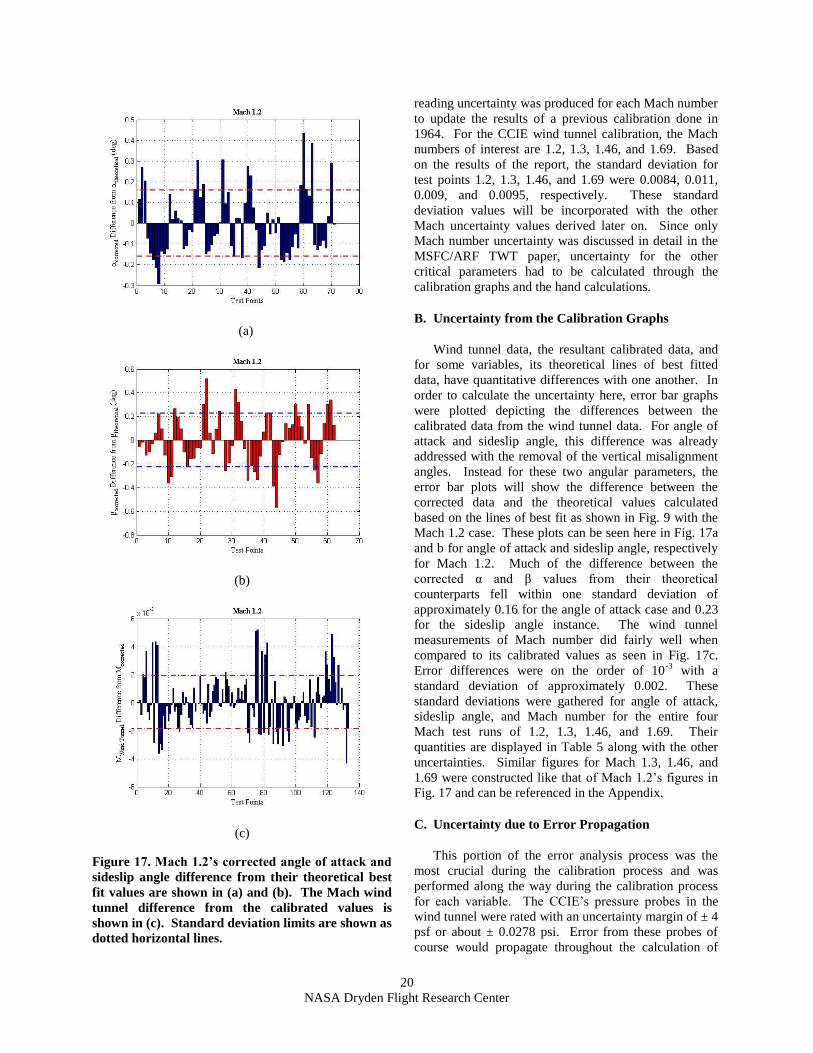
B. Uncertainty from the Calibration Graphs
Wind tunnel data, the resultant calibrated data, and
for some variables, its theoretical lines of best fitted
data, have quantitative differences with one another. In
order to calculate the uncertainty here, error bar graphs
were plotted depicting the differences between the
calibrated data from the wind tunnel data. For angle of
attack and sideslip angle, this difference was already
addressed with the removal of the vertical misalignment
angles. Instead for these two angular parameters, the
error bar plots will show the difference between the
corrected data and the theoretical values calculated
based on the lines of best fit as shown in Fig. 9 with the
Mach 1.2 case. These plots can be seen here in Fig. 17a
and b for angle of attack and sideslip angle, respectively
for Mach 1.2. Much of the difference between the
corrected α and β values from their theoretical
counterparts fell within one standard deviation of
approximately 0.16 for the angle of attack case and 0.23
for the sideslip angle instance. The wind tunnel
measurements of Mach number did fairly well when
compared to its calibrated values as seen in Fig. 17c.
Error differences were on the order of 10-3
with a
standard deviation of approximately 0.002. These
standard deviations were gathered for angle of attack,
sideslip angle, and Mach number for the entire four
Mach test runs of 1.2, 1.3, 1.46, and 1.69. Their
quantities are displayed in Table 5 along with the other
uncertainties. Similar figures for Mach 1.3, 1.46, and
1.69 were constructed like that of Mach 1.2’s figures in
Fig. 17 and can be referenced in the Appendix.
C. Uncertainty due to Error Propagation
This portion of the error analysis process was the
most crucial during the calibration process and was
performed along the way during the calibration process
for each variable. The CCIE’s pressure probes in the
wind tunnel were rated with an uncertainty margin of ± 4
psf or about ± 0.0278 psi. Error from these probes of
course would propagate throughout the calculation of
(a)
(b)
(c)
Figure 17. Mach 1.2’s corrected angle of attack and
sideslip angle difference from their theoretical best
fit values are shown in (a) and (b). The Mach wind
tunnel difference from the calibrated values is
shown in (c). Standard deviation limits are shown as
dotted horizontal lines.

21
NASA Dryden Flight Research Center
subsequent variables that are dependent upon them. With hundreds of data points for all of the four Mach test runs
and dozens of variables to calculate for each data points, using MATLAB is the logical way to perform all the
uncertainty analysis. To certify that the calculations are correct, hand calculations of error analysis were performed
at a random data point for each variable. All of the data points had an error associated with it, but the most
important critical in-flight parameters, like angle of attack, sideslip angle, Mach number, and dynamic pressure had
their uncertainties averaged resulting in a single value for each Mach test run. Their respective uncertainty values
are shown in Table 5. Sample calculations of the error analysis performed for these variables and other parameters
are available in the Appendix for reference.
D. Combine the Uncertainty Results
Uncertainties from the wind tunnel, the calibration graphs, and due to error propagation for angle of attack,
sideslip angle, Mach number, and dynamic pressure are all different. Since they were calculated independent of one
another, the uncertainties could be combined using Eq. 27,
(27)
which is based on the root-sum squared method. The combined results are shown in Table 5 below along with the
other calculated uncertainties for the other three sources for comparison. Mach number and dynamic pressure both
had the least error. Angle of attack and sideslip angle had slightly larger error values, but were acceptable. If the
vertical misalignment angle had not been removed, the error results would definitely have been much greater.
Table 5. The uncertainty values of angle of attack, α, sideslip angle, β, Mach number, and dynamic
pressure, Qbar for the wind tunnel, the calibration graphs, and the error propagation are displayed here
along with their combined results for Mach 1.2, 1.3, 1.46, and 1.69.
Mach 1.2 Mach 1.3 Mach 1.46 Mach 1.69
Wind Tunnel
α - - - -
β - - - -
Mach 0.0084 0.0110 0.0090 0.0095
Qbar - - - -
Calibration Graphs
α 0.15930 0.33860 0.23210 0.17710
β 0.22770 0.28960 0.45720 0.27320
Mach 0.00191 0.00388 0.00367 0.00340
Qbar - - - -
Error Propagation
α 0.29667 0.29695 0.31282 0.24138
β 0.30081 0.31404 0.32548 0.24402
Mach 0.00255 0.00274 0.00319 0.00353
Qbar 0.04778 0.05143 0.05851 0.07131
Combined
Uncertainty Results
α 0.33673 0.45036 0.38952 0.29938
β 0.37727 0.42719 0.56122 0.36631
Mach 0.00898 0.01198 0.01023 0.01069
Qbar 0.04778 0.05143 0.05851 0.07131

22
NASA Dryden Flight Research Center
IV. Create the In-Flight RTF Script
With the calibration completed and the uncertainty analysis taken care of, the results from the calibration could
now be implemented into the in-flight RTF script to compute critical flight parameters during the experimental flight
tests of the CCIE on the F-15B research aircraft. The script was written using MATLAB at first, but will later be
converted into RTF with the aid of the computer engineers of NASA DFRC’s Western Aeronautical Test Range
(WATR), which provides useful resources for flight research operations and low earth-orbiting missions, such as
mission control, communication, telemetry, and real-time data acquisition. Any MATLAB shortcuts, commands, or
built-in functions had to be avoided in order for the script to be compatible with RTF.
The CCIE multi-hole pressure probe will measure pressures from five different ports, P1, P2, P3, P4, and P5 as
shown in Fig. 4. During an actual flight, the five measured pressured pressures will be inputted into a function that
will make an initial estimate of the Mach number based on the given flow conditions. The average probe static
pressure, Pa will be calculated first in order to derive the static-pitot pressure ratio,
, which the Mach number is
dependent upon. From Fig. 16, the conical flow theory trend line relates the static-pitot pressure ratio to Mach
number in Eq. 28 as
. (28)
from which the estimated Mach number could be computed. The estimated Mach number and the five measured
pressures would then be inputted into a different function that will then calculate the in-flight parameters of interest.
The conical flow relationship between Mach number and the static-pitot pressure ratio shown in Eq. 28 is only valid
for Mach numbers above 1.05. As a result, for estimated Mach numbers that are below 1.05, the function will tell
Figure 18. This flowchart shows a visual representation of how the in-flight RTF script would run on the
mission control displays during a CCIE research experimental flight.

23
NASA Dryden Flight Research Center
the code to stop running and not calculate anything. If the estimated Mach number is above 1.05 and on target at the
CCIE Mach test points of 1.2, 1.3, 1.46, and 1.69, calibrated equations will be used to calculate variables, such as α,
β, Cs, and Ct, otherwise other estimated Mach numbers will prompt the in-flight function to perform an interpolation
to derive solutions for these variables. It should be noted that two values of Ct and Cs are calculated for the angle of
attack and sideslip case, respectively. However, from Fig. 10 and 11 for the total pressure coefficient and Fig. 12
and 13 for the static pressure coefficient, the values of and
as well as and
are fairly close. As a
result, the resulting averages of the angle of attack and sideslip values of both the total and static pressure
coefficients will be sufficient for the values of Ct and Cs, respectively. Afterwards, the resultant variables α, β, Cs,
and Ct would be used to calculate the static and total pressure, Ps and Po, as well as the local Mach number. This
Mach number should not be confused from the aircraft Mach number as it is based on the measured pressures of the
CCIE, which is mounted underneath the aircraft. Again, averages between the α and β values of these variables are
used to derive the final value. If the estimated Mach number and the newly derived in-flight Mach number have a
difference of less than 1%, the function would output the critical in-flight parameters to the user in mission control
and parameters include α, β, Cs, Ct, Ps, Po, M, Qbar, and the number of iterations it took to derive these solutions. If
the estimated Mach number and the in-flight Mach number calculated have a difference greater than 1%, the in-
flight Mach number becomes the new estimated Mach number and the in-flight function starts all over again until
the convergence criteria is met.
V. Current Status of the Channeled Centerbody Inlet Experiment
The CCIE test fixture is currently undergoing preparation for research flights this upcoming summer of 2011.
The aerodynamics group is performing the aerodynamic loads and CFD analysis with discussions underway to
ensure the CCIE fixture’s structural load integrity. The structures team will be involved in performing a ground
vibrations test in order to guarantee that the CCIE test fixture has an adequate flutter clearance for flight safety.
Instrumentation engineers are overseeing wiring and tubing connections and updating existing electrical design
drawing to reflect the changes. In addition, operations will be involved in outlining flight test maneuvers,
coordinating test activities, and monitoring any configuration changes. Also, WATR engineers will construct data
displays in the mission control room for all organizations involved with the project and will include implementation
the in-flight RTF script discussed earlier. Prior to the first flight, a Combined Systems Test (CST) will be performed
to confirm the F-15 aircraft functionality by verifying the control room displays, RTF code, instrumentation,
telemetry, and communication. The flights will gather information about the two CCIE configurations, one with the
channeled centerbody and one with the smooth centerbody, and comparisons will be made between the two
regarding mass flow, pressure recovery, and how well they perform with respect to the viscous CFD analysis. Post-
flight data analysis will be conducted towards the end of the year.
VI. Conclusion
Enhanced supersonic and hypersonic cruise and acceleration will depend on an effective geometric inlet design
capable of large air mass flow. The Channeled Centerbody Inlet Experiment research project done here at NASA
Dryden Flight Research Center will prove crucial in this investigation. By testing out two different configurations
with the channeled centerbody and the smooth centerbody, researchers hope to document the performance of each
centerbody and compare the results of the flight test by validating the CFD findings. If the CCIE performs well and
concurs with CFD results, the channeled centerbody concept could become a breakthrough for supersonic and
hypersonic flight.
Wind tunnel testing of the CCIE multi-hole pressure probe yielded data results for four Mach conditions of 1.2,
1.3, 1.46, and 1.69 that needed to be calibrated in order to derive in-flight parameters. This conical probe calibration
consisted of extensive steps in order to produce the desired calibrated results. By defining the probe orientation and
coordinate system, calculations were much easier to determine the pressure coefficients, like Cα, Cβ, Ct, and Cs.
Next, the vertical misalignment angle, αo and βo were determined and removed from the data set so that the location
where pressure coefficients, Cα and Cβ remain independent of roll angle at zero degrees angle of attack or sideslip in
order to reflect more like the theoretical case. Afterwards, angle of attack, sideslip angle, total and static pressure
coefficients had their equations derived to reflect their best fit trends. Flow properties were then computed to reflect
the calibrated case and static-pitot pressure ratio trends were created to determine how well the wind tunnel results
fit with the conical flow theory. The uncertainty analysis was then performed and consisted of calculating error
from three different sources, which include the wind tunnel, the calibration graphs, and error propagation with the
aid of MATLAB and self-check. The uncertainties were then combined and with the uncertainties within reasonable

24
NASA Dryden Flight Research Center
limits, the calibrated results were then assimilated into the in-flight RTF script, which will calculate critical in-flight
parameters, such as angle of attack, sideslip angle, dynamic pressure, and Mach number.
With the CCIE in preparation for its research flights, there is much anticipation of what the flight results may
turn out like. Results from this research project could contribute to a tremendous amount of new information on
how to enrich supersonic and hypersonic flight. As the world heads deeper into the 21st century, technology will
only continue to advance and improve, including the world of aeronautics. NASA Dryden Flight Research Center
has been at the forefront of aeronautics research for over 50 years and it will continue to be a place of innovation for
future enhanced aircraft performance.

25
NASA Dryden Flight Research Center
Appendix
A. Additional Calibration Figures
1) Vertical Misalignment
(a) (b)
(c) (d)
(e) (f)
Figure 19. Analogous to Fig. 4 with the Mach 1.2 case, the vertical misalignments are shown here for both
angle of attack and sideslip for Mach 1.3 (a & b), Mach 1.46 (c & d), and Mach 1.69 (e & f). Mach 1.69’s α
and β-pitch coefficient offsets, and
are very small and cannot be shown. The sizes of the
misalignments, αo and βo can be compared to that of Table 1.

26
NASA Dryden Flight Research Center
2) Vertical Misalignment Removed
(a) (b)
(c) (d)
(e) (f)
Figure 20. Like the Mach 1.2 example shown in Fig. 5, the vertical misalignment angles are removed here
for both the angle of attack and sideslip angle instances for Mach 1.3 (a & b), Mach 1.46 (c & d), and Mach
1.60 (e & f).

27
NASA Dryden Flight Research Center
3) Original α and β Comparision to Corrected α and β
(a) (b)
(c) (d)
(e) (f)
Figure 21. αoriginal and βoriginal are plotted with their respective corrected values for Mach 1.3 (a & b), Mach
1.46 (c &d ), and Mach 1.69 (e & f), similar to the plots of Mach 1.2 in Fig. 6. The separation between the
original and corrected data points represent the vertical misalignment, with Mach 1.46 having the least
bias and Mach 1.3 having the most. However, Mach 1.46’s trend is not as linear as the others.

28
NASA Dryden Flight Research Center
4) αcorrected and βcorrected Best Fit Trends
(a) (b)
(c) (d)
(e) (f)
Figure 22. The αcorrected and βcorrected best fit trends, which represents the theoretical linear relationship of
angle of attack and sideslip angle with their respective pressure coefficients, are shown here for Mach 1.3
(a & b), Mach 1.46 (c & d), and Mach 1.69 (e & f). Comparing it to Mach 1.2’s plots in Fig. 7, Mach 1.2
and 1.69 fit fairly well, while the sideslip case for Mach 1.46 seemed to exhibit a higher-order behavior.

29
NASA Dryden Flight Research Center
5) Static and Total Pressure Coefficient Comparison
(a) (b)
(c) (d)
Figure 23. Like the Mach 1.2 and 1.46 plots shown in Fig.12, the static and total pressure coefficient values
for both the angle of attack and sideslip angle cases are plotted for the Mach 1.3 (a & b) and Mach 1.69 (c
& d) simultaneously. Notice how the total pressure coefficient values of and
linger around zero
and the static pressure coefficient values of and
hover around one.

30
NASA Dryden Flight Research Center
B. Additional Calibration Uncertainty Graphs
1) Corrected Angle of Attack Difference From Theoretical
(a)
(b) (c)
Figure 24. Similar to Mach 1.2’s αcorrected difference from theoretical graph in Fig. 15a, the calibration
error bar graphs for the angle of attack case are shown here for Mach 1.3 (a), Mach 1.46 (b), and Mach
1.69 (c). Each Mach test run has differing number of test points. As seen from these figures, much of the
data results fell within the standard deviation dashed lines. The standard deviation corresponding to
these error bar graphs could be viewed in Table 5 under the calibrations graphs section.

31
NASA Dryden Flight Research Center
2) Corrected Sideslip Angle Difference From Theoretical
(a)
(b) (c)
Figure 25. Mach 1.2’s corrected sideslip error difference from its theoretical counterpart was shown in
Fig. 15b and the case for Mach 1.3 (a), Mach 1.46 (b), and Mach 1.69 (c) are shown here. Mach 1.46 had
the largest difference of all the Mach test points and from Fig. 20d, its corrected data points were a bit off
from the linear trend line, which explained why it had a wider standard deviation margin.

32
NASA Dryden Flight Research Center
3) Wind Tunnel Mach Number Difference From Corrected
(a)
(b) (c)
Figure 26. Like the error bar difference for Mach 1.2 in Fig. 15c, the error between the wind tunnel
Mach number and the corrected Mach number for Mach 1.3 (a), Mach 1.46 (b), and Mach 1.69 (c) have
small standard deviation values with all of them having deviations of less than 0.5%.

33
NASA Dryden Flight Research Center
C. Sample Error Calculations
The method that was used to calculate the uncertainties for many of the variables during the calibration are
shown here. This process was both done in MATLAB for the many test points and by hand for a random test point
to verify MATLAB’s accuracy. Results for critical parameters like α, β, M, and Qbar were shown in Table 5.
1) Error Process for Calculating Pa, Cα, Cβ, Ct, Cs, αo, , βo,
and
The trisonic wind tunnel pressure transducers’ uncertainty on the CCIE pressure probes is rated at about
dp = ± 0.0278 psi. Using Pa as an example from Eq. 1, the error for Pa should be calculated as follows:
(29)
The remaining variables could be calculated in a similar manner.
2) Error Process for Calculating Mach Number
Based on Eq. 23 and 24, the error in the calibrated Mach number for the angle of attack and sideslip angle
case could be calculated as,
(30)

34
NASA Dryden Flight Research Center
3) Error Process for Calculating Qbar-true
Based on Eq. 25 and 26, the error in the calibrated dynamic pressure can be calculated as,
(31)
D. MATLAB In-Flight RTF Script
1) Function to Estimate Initial Mach Number (est_mach.m)
function [est_mach] = est_mach(P1,P2,P3,P4,P5) % %EST_MACH - Calculate the initial estimate of the Mach number based on % the conical static-pitot pressure ratio vs. Mach relation % from the in-flight measured pressures obtained. % % EST_MACH(P1,P2,P3,P4,P5) - Input in-flight measured pressures % results to calculate the static-pitot pressure ratio, which in turn % outputs an intial estimate of Mach number. The initial guess will % then be inputted into the INFLIGHT.m function to calculate the % remainder parameters of interest and the corrected Mach number based % on the calibration tables. %
% By: Samson S. Truong
% Edited by: Mike Frederick %========================================================================== % Nomenclature % % est_mach - Initial Estimate of Mach Number % Pratio - Static-Pitot Pressure Ratio (Pa/P1 or Pa/Pt2) % P1 - Measured Total Pressure (psi) % P2,P3,P4,P5 - Measured Static Pressures (psi) % Pa - Average Measured Static Pressure (psi) %========================================================================== %-------------------------------------------------------------------------- %Calculate Average Static Pressure, Pa %-------------------------------------------------------------------------- Pa = 0.25*(P2+P3+P4+P5); %-------------------------------------------------------------------------- %Calculate Static-Pitot Pressure Ratio, Pa/P1 (or) Pa/Pt2 %-------------------------------------------------------------------------- Pratio = Pa./P1;

35
NASA Dryden Flight Research Center
%-------------------------------------------------------------------------- %Calculate Estimated Mach %-------------------------------------------------------------------------- est_mach = -13.7965.*Pratio.^3 + 21.1538.*Pratio.^2 - 12.5144.*Pratio + 3.8167; %-------------------------------------------------------------------------- %Call out In-Flight Function (inflight.m) %-------------------------------------------------------------------------- [iter,alpha,beta,Ca,Cb,Cs,Ct,Ps,Pt,MACH,dm,QBAR] = inflight(P1,P2,P3,P4,P5,est_mach)
2) Function to Calculate Critical In-Flight Parameters (inflight.m)
function [iter,alpha,beta,Ca,Cb,Cs,Ct,Ps,Pt,MACH,dm,QBAR] = inflight(P1,P2,P3,P4,P5,est_mach)
%
%INFLIGHT - Calculate flight parameters of interests using in-flight
% measured pressures and interpolating results in-between
% calibrated test points
%
% INFLIGHT(P1,P2,P3,P4,P5,mach) - Input in-flight measured pressures &
% initial Mach number guess, to output angle of attack, sideslip
% angle, MACH, and other significant flight data parameters using
% interpolation of the test points of interests at Machs 1.2, 1.3,
% 1.46, & 1.69.
%
% By: Samson S. Truong
% Edited by: Mike Frederick %==========================================================================
% Nomenclature
%
% alpha - Angle of Attack (deg)
% beta - Sideslip Angle (deg)
% Ca - Pressure Coefficient w/respect to Angle of Attack
% Cb - Pressure Coefficient w/respect to Sideslip Angle
% Cs - Average Static Pressure Coefficient
% Csa - Static Pressure Coefficient w/respect to Angle of Attack
% Csb - Static Pressure Coefficient w/respect to Sideslip Angle
% Ct - Average Total Pressure Coefficient
% Cta - Total Pressure Coefficient w/respect to Angle of Attack
% Ctb - Total Pressure Coefficient w/respect to Sideslip Angle
% dm - Change in Mach Number
% est_mach - Initial Estimate of Mach Number
% gamma - Ratio of Specific Heats
% iter - # of Iterations for Solution Convergence
% MACH - Average Mach Number
% macha - Mach Number w/respect to Angle of Attack
% machb - Mach Number w/respect to Sideslip Angle
% P1 - Measured Total Pressure (psi)
% P2,P3,P4,P5 - Measured Static Pressures (psi)
% Pa - Average Measured Static Pressure (psi)
% Ps - Average In-Flight Static Pressure (psi)
% Psa - In-Flight Static Pressure w/respect to Angle of Attack (psi)
% Psb - In-Flight Static Pressure w/respect to Sideslip Angle (psi)
% Pt - Average In-Flight Total Pressure (psi)
% Pta - In-Flight Total Pressure w/respect to Angle of Attack (psi)

36
NASA Dryden Flight Research Center
% Ptb - In-Flight Total Pressure w/respect to Sideslip Angle (psi)
% pQBAR - Pseudo-Dynamic Pressure (psi)
% QBAR - Average In-Flight Dynamic Pressure (psf)
% QBARa - In-Flight Dynamic Pressure w/respect to Angle of Attack (psf)
% QBARb - In-Flight Dynamic Pressure w/respect to Sideslip Angle (psf)
%
%==========================================================================
%Ratio of Specific Heat Coefficient
gamma = 1.4;
%Calculate Average Static Pressure, Pa
Pa = 0.25*(P2+P3+P4+P5);
%Calculate Pseudo Dynamic Pressure, pQBAR
pQBAR = P1 - Pa;
%Pressure Coefficient w/respect to Angle of Attack, Ca:
Ca = (P3-P5)./(P1-Pa);
%Pressure Coefficient w/respect to Sideslip Angle, Cb:
Cb = (P4-P2)./(P1-Pa);
%% Begin While Loop
i = 1;
stop = 0;
if est_mach < 1.05
disp('Estimated Mach Value is below 1.05. Code Terminated.')
end
while stop == 0
if est_mach < 1.05
break
end
%--------------------------------------------------------------------------
%Calculate solutions from calibration tables.
%--------------------------------------------------------------------------
% l = low end & h = high end
if est_mach <= 1.20
alpha1_2(i) = 89.1385*Ca + 0.7089;
beta1_2(i) = 90.4277*Cb + 0.28410;
Csa1_2(i) = -2.6378*Ca^2 - 0.043026*Ca + 1.0786;
Csb1_2(i) = -2.3004*Cb^2 - 0.023978*Cb + 1.0776;
Cta1_2(i) = 7.9419e-04*Ca - 0.015497;
Ctb1_2(i) = -0.0010123*Cb - 0.015517;
elseif (est_mach > 1.20) && (est_mach < 1.30)
alphal(i) = 89.1385*Ca + 0.7089;
alphah(i) = 94.6015*Ca + 0.5037;
betal(i) = 90.4277*Cb + 0.28410;
betah(i) = 100.0237*Cb + 0.2179;
Csal(i) = -2.6378*Ca^2 - 0.043026*Ca + 1.0786;
Csah(i) = -2.7522*Ca^2 - 0.021851*Ca + 1.0765;
Csbl(i) = -2.3004*Cb^2 - 0.023978*Cb + 1.0776;

37
NASA Dryden Flight Research Center
Csbh(i) = -2.7696*Cb^2 + 0.023859*Cb + 1.0756;
Ctal(i) = 7.9419e-04*Ca - 0.015497;
Ctah(i) = 0.43365*Ca^2 - 1.2153e-04*Ca - 0.046727;
Ctbl(i) = -0.0010123*Cb - 0.015517;
Ctbh(i) = 0.38196*Cb^2 + 0.0045245*Cb - 0.047481;
elseif est_mach == 1.30
alpha1_3(i) = 94.6015*Ca + 0.5037;
beta1_3(i) = 100.0237*Cb + 0.2179;
Csa1_3(i) = -2.7522*Ca^2 - 0.021851*Ca + 1.0765;
Csb1_3(i) = -2.7696*Cb^2 + 0.023859*Cb + 1.0756;
Cta1_3(i) = 0.43365*Ca^2 - 1.2153e-04*Ca - 0.046727;
Ctb1_3(i) = 0.38196*Cb^2 + 0.0045245*Cb - 0.047481;
elseif (est_mach > 1.3) && (est_mach < 1.46)
alphal(i) = 94.6015*Ca + 0.5037;
alphah(i) = 108.0175*Ca + 0.4175;
betal(i) = 100.0237*Cb + 0.2179;
betah(i) = 112.3877*Cb + 0.1192;
Csal(i) = -2.7522*Ca^2 - 0.021851*Ca + 1.0765;
Csah(i) = 8.5362*Ca^3 - 3.3971*Ca^2 - 0.038168*Ca + 1.0618;
Csbl(i) = -2.7696*Cb^2 + 0.023859*Cb + 1.0756;
Csbh(i) = 17.772*Cb^3 - 3.2717*Cb^2 - 0.021265*Cb + 1.0618;
Ctal(i) = 0.43365*Ca^2 - 1.2153e-04*Ca - 0.046727;
Ctah(i) = 0.0086243*Ca - 0.090352;
Ctbl(i) = 0.38196*Cb^2 + 0.0045245*Cb - 0.047481;
Ctbh(i) = 0.024073*Cb - 0.090279;
elseif est_mach == 1.46;
alpha1_46(i) = 108.0175*Ca + 0.4175;
beta1_46(i) = 112.3877*Cb + 0.1192;
Csa1_46(i) = 8.5362*Ca^3 - 3.3971*Ca^2 - 0.038168*Ca + 1.0618;
Csb1_46(i) = 17.772*Cb^3 - 3.2717*Cb^2 - 0.021265*Cb + 1.0618;
Cta1_46(i) = 0.0086243*Ca - 0.090352;
Ctb1_46(i) = 0.024073*Cb - 0.090279;
elseif (est_mach > 1.46) && (est_mach < 1.69)
alphal(i) = 108.0175*Ca + 0.4175;
alphah(i) = 99.9231*Ca + 0.1318;
betal(i) = 112.3877*Cb + 0.1192;
betah(i) = 100.8961*Cb + 0.0871;
Csal(i) = 8.5362*Ca^3 - 3.3971*Ca^2 - 0.038168*Ca + 1.0618;
Csah(i) = -1.3094*Ca^2 - 0.024019*Ca + 1.045;
Csbl(i) = 17.772*Cb^3 - 3.2717*Cb^2 - 0.021265*Cb + 1.0618;
Csbh(i) = -0.78067*Cb^2 + 0.0078296*Cb + 1.0452;
Ctal(i) = 0.0086243*Ca - 0.090352;
Ctah(i) = 0.72013*Ca^2 - 0.010757*Ca - 0.22335;
Ctbl(i) = 0.024073*Cb - 0.090279;
Ctbh(i) = 0.96616*Cb^2 + 0.012028*Cb - 0.22493;
elseif est_mach >= 1.69
alpha1_69(i) = 99.9231*Ca + 0.1318;
beta1_69(i) = 100.8961*Cb + 0.0871;
Csa1_69(i) = -1.3094*Ca^2 - 0.024019*Ca + 1.045;
Csb1_69(i) = -0.78067*Cb^2 + 0.0078296*Cb + 1.0452;
Cta1_69(i) = 0.72013*Ca^2 - 0.010757*Ca - 0.22335;
Ctb1_69(i) = 0.96616*Cb^2 + 0.012028*Cb - 0.22493;
end

38
NASA Dryden Flight Research Center
%--------------------------------------------------------------------------
%Interpolate solutions for alpha, beta, Csa, Csb, Cta, & Ctb
%(if between calibrated test points)
%--------------------------------------------------------------------------
if est_mach <= 1.20
alpha(i) = alpha1_2(i);
beta(i) = beta1_2(i);
Csa(i) = Csa1_2(i);
Csb(i) = Csb1_2(i);
Cs(i) = 0.5*(Csa(i) + Csb(i));
Cta(i) = Cta1_2(i);
Ctb(i) = Ctb1_2(i);
Ct(i) = 0.5*(Cta(i) + Ctb(i));
elseif (est_mach > 1.20) && (est_mach < 1.30)
Mh = 1.3;
Ml = 1.2;
alpha(i) = alphal(i) + ((est_mach - Ml)/(Mh - Ml))*(alphah(i) - alphal(i));
beta(i) = betal(i) + ((est_mach - Ml)/(Mh - Ml))*(betah(i) - betal(i));
Csa(i) = Csal(i) + ((est_mach - Ml)/(Mh - Ml))*(Csah(i) - Csal(i));
Csb(i) = Csbl(i) + ((est_mach - Ml)/(Mh - Ml))*(Csbh(i) - Csbl(i));
Cs(i) = 0.5*(Csa(i) + Csb(i));
Cta(i) = Ctal(i) + ((est_mach - Ml)/(Mh - Ml))*(Ctah(i) - Ctal(i));
Ctb(i) = Ctbl(i) + ((est_mach - Ml)/(Mh - Ml))*(Ctbh(i) - Ctbl(i));
Ct(i) = 0.5*(Cta(i) + Ctb(i));
elseif est_mach == 1.30
alpha(i) = alpha1_3(i);
beta(i) = beta1_3(i);
Csa(i) = Csa1_3(i);
Csb(i) = Csb1_3(i);
Cs(i) = 0.5*(Csa(i) + Csb(i));
Cta(i) = Cta1_3(i);
Ctb(i) = Ctb1_3(i);
Ct(i) = 0.5*(Cta(i) + Ctb(i));
elseif (est_mach > 1.3) && (est_mach < 1.46)
Mh = 1.46;
Ml = 1.3;
alpha(i) = alphal(i) + ((est_mach - Ml)/(Mh - Ml))*(alphah(i) - alphal(i));
beta(i) = betal(i) + ((est_mach - Ml)/(Mh - Ml))*(betah(i) - betal(i));
Csa(i) = Csal(i) + ((est_mach - Ml)/(Mh - Ml))*(Csah(i) - Csal(i));
Csb(i) = Csbl(i) + ((est_mach - Ml)/(Mh - Ml))*(Csbh(i) - Csbl(i));
Cs(i) = 0.5*(Csa(i) + Csb(i));
Cta(i) = Ctal(i) + ((est_mach - Ml)/(Mh - Ml))*(Ctah(i) - Ctal(i));
Ctb(i) = Ctbl(i) + ((est_mach - Ml)/(Mh - Ml))*(Ctbh(i) - Ctbl(i));
Ct(i) = 0.5*(Cta(i) + Ctb(i));
elseif est_mach == 1.46;
alpha(i) = alpha1_46(i);
beta(i) = beta1_46(i);
Csa(i) = Csa1_46(i);
Csb(i) = Csb1_46(i);
Cs(i) = 0.5*(Csa(i) + Csb(i));
Cta(i) = Cta1_46(i);
Ctb(i) = Ctb1_46(i);
Ct(i) = 0.5*(Cta(i) + Ctb(i));
elseif (est_mach > 1.46) && (est_mach < 1.69)
Mh = 1.69;
Ml = 1.46;

39
NASA Dryden Flight Research Center
alpha(i) = alphal(i) + ((est_mach - Ml)/(Mh - Ml))*(alphah(i) - alphal(i));
beta(i) = betal(i) + ((est_mach - Ml)/(Mh - Ml))*(betah(i) - betal(i));
Csa(i) = Csal(i) + ((est_mach - Ml)/(Mh - Ml))*(Csah(i) - Csal(i));
Csb(i) = Csbl(i) + ((est_mach - Ml)/(Mh - Ml))*(Csbh(i) - Csbl(i));
Cs(i) = 0.5*(Csa(i) + Csb(i));
Cta(i) = Ctal(i) + ((est_mach - Ml)/(Mh - Ml))*(Ctah(i) - Ctal(i));
Ctb(i) = Ctbl(i) + ((est_mach - Ml)/(Mh - Ml))*(Ctbh(i) - Ctbl(i));
Ct(i) = 0.5*(Cta(i) + Ctb(i));
elseif est_mach >= 1.69
alpha(i) = alpha1_69(i);
beta(i) = beta1_69(i);
Csa(i) = Csa1_69(i);
Csb(i) = Csb1_69(i);
Cs(i) = 0.5*(Csa(i) + Csb(i));
Cta(i) = Cta1_69(i);
Ctb(i) = Ctb1_69(i);
Ct(i) = 0.5*(Cta(i) + Ctb(i));
end
%--------------------------------------------------------------------------
%Calculate Static & Total Pressures
%--------------------------------------------------------------------------
Psa(i) = P1 - Csa(i)*pQBAR;
Psb(i) = P1 - Csb(i)*pQBAR;
Ps(i) = 0.5*(Psa(i) + Psb(i));
Pta(i) = P1 - Cta(i)*pQBAR;
Ptb(i) = P1 - Ctb(i)*pQBAR;
Pt(i) = 0.5*(Pta(i) + Ptb(i));
%--------------------------------------------------------------------------
%Calculate Mach Number & Check for Convergence
%--------------------------------------------------------------------------
macha(i) = ((2/(gamma-1))*(((Pta(i)/Psa(i))^((gamma-1)/gamma)) - 1))^0.5;
machb(i) = ((2/(gamma-1))*(((Ptb(i)/Psb(i))^((gamma-1)/gamma)) - 1))^0.5;
mach(i) = 0.5*(macha(i) + machb(i));
est_mach = mach(i);
%--------------------------------------------------------------------------
%Output Final Solutions
%--------------------------------------------------------------------------
if i > 1
dm(i,1) = ((mach(i) - mach(i-1))/mach(i))*100;
if abs(dm(i,1)) > 0.01
stop = 0;
else
stop = 1;
iter = length(mach);
alpha = alpha(end);
beta = beta(end);
Cs = Cs(end);
Ct = Ct(end);
Ps = Ps(end);
Pt = Pt(end);
MACH = mach(end);
QBARa = 0.5*gamma*Psa(end)*macha(end)^2;

40
NASA Dryden Flight Research Center
QBARb = 0.5*gamma*Psb(end)*machb(end)^2;
QBAR = (0.5*(QBARa(end) + QBARb(end)))*144;
stop = 1;
end
end
i = i + 1;
end

41
NASA Dryden Flight Research Center
Acknowledgements
I would like to thank my supervisor and branch chief, Jennifer Cole for allowing me the opportunity to work in
the Aerodynamic & Propulsion Branch for the Spring 2011 term. In addition, I would sincerely want to thank my
Cooperative Education Experience mentor and senior project industry advisor, Mike Frederick for all of his help and
advice throughout the duration of my project. Also, I want to thank my school advisor, Dr. Eric Mehiel, head of Cal
Poly San Luis Obispo’s Aerospace Engineering Department for monitoring my progress during my stay here at
NASA DFRC. Furthermore, I would like to thank the entire staff at NASA Dryden Flight Research Center and the
F-15B Project Team for making my stay here over the past two years an enjoyable and educational experience.
Finally, I want to thank the most important people in my life, my parents and my sister, for their unending support
throughout my college education.
References
[1] Weir, Lois J., Sanders, Bobby W., Meleason, Edward T., and Podleski, Steve D., “Flight Testing of a New Design Concept
for Axisymmetric Inlets,” TechLand Research, Inc., TechLand Research Report Number TRR-020406, North Olmsted, OH, Feb.
2006.
[2] Weir, Lois J., Sanders, Bobby W., and Vachon, Michael J., “A New Design Concept for Supersonic Axisymmetric Inlets,”
AIAA-2002-3775.
[3] Frederick, Mike, and St. John, Clint, “Propulsion Flight Test Fixture (PFTF): Channeled Centerbody Inlet Experiment (CCIE)
– Flight Tests of the Channeled Centerbody Inlet Concept, Objectives and Requirements Document (ORD), F-15B Project,”
NASA CCIE ORD Rev. 6, Edwards, CA, Feb. 2011.
[4] & [15] Andrews, Mark F., Abernathy, Michael, and Pritchett, Victor, “Calibration of Mach Number Set Points for the MSFC
14 × 14-Inch Trisonic Wind Tunnel,” Report No.: ESTSG-FY10-01636, Jacobs Engineering, Ducommun Miltec, and NASA,
May 2010.
[5] “Dryden 5-Hole Probe Test Brief,” NASA DFRC, Edwards, CA, Jun. 2010.
[6], [9] & [10] Zeiger, Matthew D. and Schaeffler, Norman W., “Correcting Multi-Hole Probe Alignment Bias Errors Post-
Calibration,” Aeroprobe Corporation, Blacksburg, VA, AIAA-2001-0900.
[7] & [13] Centolanzi, Frank J, “Characteristics of a 40° Cone for Measuring Mach Number, Total Pressure, and Flow Angles at
Supersonic Speeds,” NACA TN 3967, May 1957.
[8] Zeiger, M. D., Chalmeta, L. P., and D. P. Telionis, “Tip Geometry Effects on Calibration and Performance of Seven-Hole
Probes,” Aeroprobe Corporation & Virginia Polytechnic Institute and State University, AIAA-1998-2810.
[11] Anderson, John D., Fundamentals of Aerodynamics, 5th edition, McGraw-Hill, New York, 2011, pp.826-827.
[12] John, James E. and Keith, Theo G, Gas Dynamics, 3rd Edition, Pearson Prentice Hall, Upper Saddle River, NJ, 2006, pp. 82 -
88.
[14] Ames Research Staff, “Equations, Tables, and Charts for Compressible Flow,” NACA Report 1135, 1953.
Recommended


![Performance of IBA New Conical Shaped Niobium [18O] Water ... · Vienna sept 2010, poster #9, session P13. Table 2: Results Summary Conical 6 Conical 8 Conical 12 Conical 16 Insert](https://img.pdfslide.net/doc/110x75/5f901a7319a03054823be5c3/performance-of-iba-new-conical-shaped-niobium-18o-water-vienna-sept-2010.jpg)