Bending of Curved Beams – Strength of Materials Approach
N
M
V
r
θ
cross-section must be symmetric but does not have to be rectangular
assume plane sections remain plane and just rotate about the neutral axis, as for a straight beam, and that the only significant stress is the hoop stress
θθσ
θθσ

N
M
centroid neutral axis
nRR
r
R = radius to centroidRn = radius to neutral axisr = radius to general fiber in the beam
N, M = normal force and bending momentcomputed from centroid
θ∆
A
B
A
B
P
P
nR r−
φ∆
( ) 1n nR r Rlel r rθθ
φω
θφωθ
− ∆∆ ⎛ ⎞= = = −⎜ ⎟∆ ⎝ ⎠∆
=∆
Let ∆φ = rotation of thecross-section
Reference: Advanced Mechanics of Materials : Boresi, Schmidt, andSidebottom

From Hooke’s law
1nREe Erθθ θθσ ω ⎛ ⎞= = −⎜ ⎟
⎝ ⎠
Then the normal force is given by
( )
nA A A
n m
dAN dA E R dAr
E R A A
θθσ ω
ω
⎡ ⎤= = −⎢ ⎥
⎣ ⎦= −
∫ ∫ ∫
wherem
A
dAAr
= ∫ has the dimensions of a length
Similarly, for the moment ( )
( )
( )
1
A
n
A
n nA A A A
n m
M R r dA
RE R r dAr
dAE R R R dA R dA rdAr
E R RA A
θθσ
ω
ω
ω
= −
⎛ ⎞= − −⎜ ⎟⎝ ⎠
⎡ ⎤= − − +⎢ ⎥
⎣ ⎦= −
∫
∫
∫ ∫ ∫ ∫

( )( )
n m
n m
M E R RA A
N E R A A
ω
ω
= −
= −
from (1)
(1)
(2)
nm
ME RRA A
ω =−
from (2) ( )n m
m
m
N E R A E AMA E A
RA A
ω ω
ω
= −
= −−
so solving for Eω( )
m
m
MA NEA RA A A
ω = −−
1n
n
REe Er
E R Er
θθ θθσ ω
ω ω
⎛ ⎞= = −⎜ ⎟⎝ ⎠
= −
Recall, the stress is given by
so using expressions for ,nE R Eω ω

we obtain the hoop stress in the form
( )( )
m
m
M A rANA Ar RA Aθθσ
−= +
−
axialstress
bendingstress
nr R=
setting the total stress = 0 gives
0N ≠
( )0m m
AMrA M N A RAθθσ =
=+ −
0N =
setting the bending stress = 0 and gives nm
ARA
=
which in general is not at the centroid
location of theneutral axis

For composite areas
A1
A2
1R2R
i
m mi
i i
i
A A
A A
R AR
A
=
=
=
∑∑∑∑radii to centroids
areas

Example
P
P
100 mm30 mm
For a square 50x50 mm cross-section, find the maximum tensile and compressive stress if P = 9.5 kN and plot the total stress across the cross-section

P = 9500 N
MN
155 mm
a
c
b
( )
2
lnm
A b c aa cR
cA ba
= −
+=
⎛ ⎞= ⎜ ⎟⎝ ⎠
a = 30 mmb = 50 mmc = 80 mm
so we have( )( ) 250 50 2500
8050ln 49.0430
80 30 552
m
A mm
A mm
R mm
= =
⎛ ⎞= =⎜ ⎟⎝ ⎠
+= =
2500 5149.04nR mm= =
T C

max tensile stress is at r = 30 mm
( )( )
( )( ) ( )( )( )( ) ( )( )155 9500 2500 30 49.049500
2500 2500 30 55 49.04 2500
106.2
m
m
M A rANA Ar RA A
MPa
θθσ−
= +−
−⎡ ⎤⎣ ⎦= +−⎡ ⎤⎣ ⎦
=
max compressive stress is at r = 80 mm
( )( )
( )( ) ( )( )( )( ) ( )( )155 9500 2500 80 49.049500
2500 2500 80 55 49.04 2500
49.3
m
m
M A rANA Ar RA A
MPa
θθσ−
= +−
−⎡ ⎤⎣ ⎦= +−⎡ ⎤⎣ ⎦
= −

>> r= linspace(30, 80, 100);>> stress = 3.8 + 589*(2500 - 49.04.*r)./(197.2*r);>> plot(r, stress)
30 35 40 45 50 55 60 65 70 75 80-60
-40
-20
0
20
40
60
80
100
120
radius, r
stre
ss

Comparison with Airy Stress Function Results
Consider a rectangular beam under pure moment
a
b
r
MM
thickness = t
R
h
Note: ( )( )
( )( )
/ 1/
2 / 1
2 / 1/
2 / 1
b aR h
b a
R hb a
R h
+=
−
+=
−
y

2 2 2
2
4 ln ln ln 1M a b b b r a r bNta r a a a a b a aθθσ
⎡ ⎤⎛ ⎞ ⎛ ⎞ ⎛ ⎞ ⎛ ⎞ ⎛ ⎞ ⎛ ⎞= − + − + −⎢ ⎥⎜ ⎟ ⎜ ⎟ ⎜ ⎟ ⎜ ⎟ ⎜ ⎟ ⎜ ⎟⎝ ⎠ ⎝ ⎠ ⎝ ⎠ ⎝ ⎠ ⎝ ⎠ ⎝ ⎠⎢ ⎥⎣ ⎦
From Airy Stress Function
2 22 2
1 4 lnb b bNa a a
⎡ ⎤ ⎡ ⎤⎛ ⎞ ⎛ ⎞ ⎛ ⎞= − −⎢ ⎥⎜ ⎟ ⎜ ⎟ ⎜ ⎟⎢ ⎥⎝ ⎠ ⎝ ⎠ ⎝ ⎠⎣ ⎦⎢ ⎥⎣ ⎦
Strength Approach
( )( )
ln
/ 2
mbA ta
A t b a
R a b
⎛ ⎞= ⎜ ⎟⎝ ⎠
= −
= +
( )( )
( )
( ) ( ) ( )
2
ln
ln2
2 1 ln
1 2 1 1 ln
m
m
M A rAAr RA A
bM b a ra
a b bt r b a b aa
b r bMa a a
r b b b bt aa a a a a
θθσ− −
=−
⎡ ⎤⎛ ⎞− − − ⎜ ⎟⎢ ⎥⎝ ⎠⎣ ⎦=+⎡ ⎤⎛ ⎞− − −⎜ ⎟⎢ ⎥
⎝ ⎠⎣ ⎦⎡ ⎤⎛ ⎞ ⎛ ⎞− −⎜ ⎟ ⎜ ⎟⎢ ⎥⎝ ⎠ ⎝ ⎠⎣ ⎦=⎡ ⎤⎛ ⎞⎛ ⎞ ⎛ ⎞ ⎛ ⎞ ⎛ ⎞− − − +⎜ ⎟⎜ ⎟ ⎜ ⎟ ⎜ ⎟ ⎜ ⎟⎢ ⎥⎝ ⎠⎝ ⎠ ⎝ ⎠ ⎝ ⎠ ⎝ ⎠⎣ ⎦
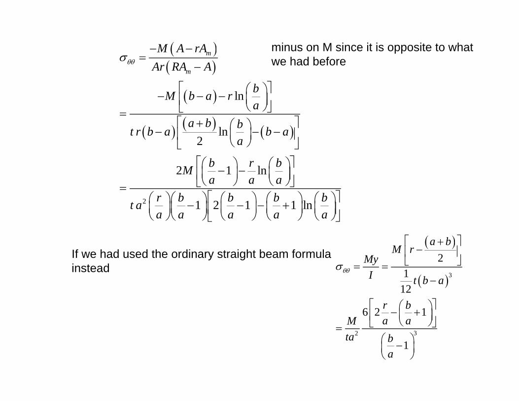
If we had used the ordinary straight beam formulainstead
( )
( )3
32
21
12
6 2 1
1
a bM r
MyI t b a
r ba aM
ta ba
θθσ
+⎡ ⎤−⎢ ⎥
⎣ ⎦= =−
⎡ ⎤⎛ ⎞− +⎜ ⎟⎢ ⎥⎝ ⎠⎣ ⎦=⎛ ⎞−⎜ ⎟⎝ ⎠
minus on M since it is opposite to what we had before

Comparison of the ratio of the max bending stresses
0.93310.99945.0
0.88810.99863.0
0.83130.99732.0
0.77370.99611.5
0.65450.99701.0
0.52621.01240.75
0.43901.04550.65
Strength/elasticityStraight beam formula My/I
Strength/elasticityCurved beamformula
R/h
R
h
y

Compare bending stress distributions at the smallest R/h value
1 2 3 4 5 6 7 8-0.35
-0.3
-0.25
-0.2
-0.15
-0.1
-0.05
0
0.05
0.1
0.15
r/a
norm
aliz
ed s
tress
solid curve – Airy stress function (elasticity)dashed blue – Curved Strength formuladashed red – Straight beam formula
R/h = 0.65 (b/a = 7.667)

% beam_compare.mm=1;Rhvals = [0.65 0.75 1.0 1.5 2.0 3.0 5.0]; % R/h ratios to considerfor Rh = Rhvalsba = (1+2*Rh)/(2*Rh -1); %corresponding b/a valuesra= linspace(1, ba, 100); % r/a valuesN=(ba^2-1)^2 -4*ba^2*(log(ba))^2;% Airy function flexure stress expressionpa =4*(-(ba./ra).^2.*log(ba)+(ba)^2.*log(ra./ba) - log(ra) +(ba)^2 -1)./N; % Curved beam strength expression for flexure stressps = 2*((ba-1)-ra.*log(ba))./(ra.*(ba-1).*(2.*(ba-1) -(ba+1).*log(ba)));% Straight beam flexure formula My/Ipb = 6*(2*ra-(ba+1))./((ba-1)^3);%obtain ratio of max stresses Curved beam Strength formula/Airyratio1(m) = max(abs(ps))/max(abs(pa));%obtain ratio of max stresses: Straight beam strength formula/Airyratio2(m) = max(abs(pb))/max(abs(pa));m=m+1;end% Now plot stress distributions for smallest R/h valueRh=0.65ba = (1+2*Rh)/(2*Rh -1); %corresponding b/a valuesra= linspace(1, ba, 100);N=(ba^2-1)^2 -4*ba^2*(log(ba))^2;pa =4*(-(ba./ra).^2.*log(ba)+(ba)^2.*log(ra./ba) - log(ra) +(ba)^2 -1)./N; ps = 2*((ba-1)-ra.*log(ba))./(ra.*(ba-1).*(2.*(ba-1) -(ba+1).*log(ba)));pb = 6*(2*ra-(ba+1))./((ba-1)^3);plot(ra, pa)hold onplot(ra, ps, '--b')plot(ra, pb, '--r')xlabel('r/a')ylabel( 'normalized stress')hold off

Comparison with Bickford’s expression (pure bending)
( ) 211/
kM MyA ky I
k R
θθσ = − −+
=
R
r
centroid
y
y−
First note that
0A
ydA =∫
Here, y is distance from the centroid
so ( ) 22
1
1 / 1 01 / 1 / 1 /A A A
y y R IydA y dAdA Iy R y R R y R R+
= + = + =+ + +∫ ∫ ∫
1
2
2
1 /
1 /
A
A
ydAIy R
y dAIy R
=+
=+
∫
∫21
IIR
= −
R r y− = −
or r y R= +

mA A
dA dARA R Rr y R
= =+∫ ∫
( )( )
1
A A A A
m
y R y dAA dA dA dA Ry R y R y R
I RAR
+= = = +
+ + +
= +
∫ ∫ ∫ ∫
1 /I R
Thus, ( ) 1 2 /mR RA A I I R− = − =

( ) 211/
kM MyA ky I
k R
θθσ = − −+
=
Now, start with Bickford’s expression
( )( )( )
( ) ( )( ) ( )
( )
( )( )( )( )
2
22
2
2 32
2 2
2 22
2 2
222
2 2
2 32
22
1
//
yRMAR y R I
y R I yARM
y R ARI
y R I y R AR ARMy R ARI y R ARI
I AR RMARI y R I
I ARRMy R I ARI
A y R I AR RM
y R AI R
θθσ⎡ ⎤
= − +⎢ ⎥+⎣ ⎦⎡ ⎤+ +
= − ⎢ ⎥+⎣ ⎦⎡ ⎤+ + +
= − −⎢ ⎥+ +⎣ ⎦⎡ ⎤+
= − −⎢ ⎥+⎣ ⎦⎡ ⎤+
= −⎢ ⎥+⎣ ⎦⎡ ⎤− + +⎢ ⎥=
+⎢ ⎥⎣ ⎦
same terms added in and subtracted out

( ) ( )( )
2 32
22
//
A y R I AR RM
y R AI Rθθσ⎡ ⎤− + +⎢ ⎥=
+⎢ ⎥⎣ ⎦
but 22 /mRA A I R− = so ( )2 3
2 /mA I AR R= +
and we find
y R r+ =
( )m
m
A rAr RA A Aθθσ⎡ ⎤−
= ⎢ ⎥−⎣ ⎦
which agrees with our previous expression
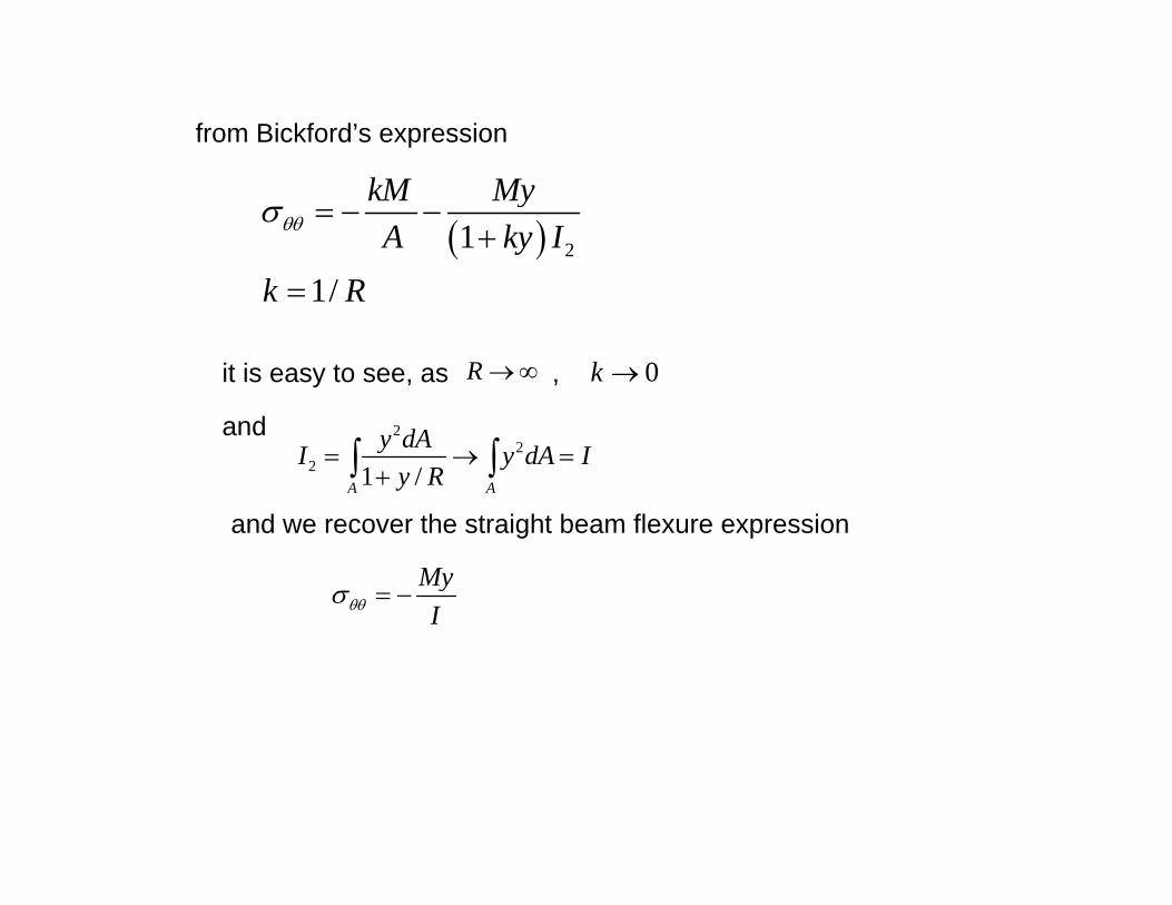
from Bickford’s expression
( ) 211/
kM MyA ky I
k R
θθσ = − −+
=
it is easy to see, as , R →∞ 0k →
and 22
2 1 /A A
y dAI y dA Iy R
= → =+∫ ∫
and we recover the straight beam flexure expression
MyIθθσ = −
Recommended